Moiré pattern assisted geometric resonant tunneling in disordered twisted bilayer graphene
Abstract
We investigate the mesoscopic transport through a twisted bilayer graphene (TBG) consisting of a clean graphene nanoribbon on the bottom and a disordered graphene disc on the top. We show that, with strong top-layer disorder the transmission through such a device shows a sequence of resonant peaks with respect to the rotation angle , where at the resonance angles the disc region contains one giant hexagonal moiré supercell. A further investigation shows that the value of shows negligible dependence on the disorder strength, the Fermi energy, and the shape distortion, indicating the resonance is a robust geometric feature of the moiré supercell. We explain this geometric resonance based on the bound states formed inside the moiré supercell, with their averaged local density of states dominating at the AA stacking region while minimizing at the AB stacking region. By increasing the interlayer distance, the peak becomes less pronounced which further confirms the role of interlayer coupling. The results presented here suggest a new mechanism to tune the quantum transport signal through the twist angle in disordered moiré systems.
I Introduction
Twisted bilayer graphene (TBG), a graphene bilayer stacked with a rotation angle , has received tremendous research interest since its first experimental observations on superconductor and Mott insulator phases YCao2018SC; YCao2018CorrelatedInsulator at the first magic angle . The interesting strong correlation phenomenon existing in a simple carbon-based two-dimensional (2D) structure, provides an exciting platform for investigating strong correlation physics Wong2020ElectronicTransition; Andrei2020TBG, and new experimental techniques in exploring the mechanism of high- superconductors Lee2019SpinTripletSC; Balents2020Superconductivity; Kennes2018Superconductivity; W2019Superconducting; Gu2020Superconductivity; Fischer2021Pairing; Liu2018Superconductivity. A small twist angle generates a giant moiré pattern with the moiré periodicity scaling inversely with , and simultaneously a reduced mini Brillouin zone. The Fermi velocity at the Dirac point is renormalized by the twist angle and approaches zero at the magic angles Santos2007GrapheneBilayer; Bistritzer2010MorieBands; Santos2012ContinuumModel, which induces flat bands Morell2010FlatBands where strong electron-electron correlation dominates and many other interesting macroscopic quantum phases arise Wong2020ElectronicTransition; Andrei2020TBG, such as ferromagnetism Sharpe2019Ferromagnetism; Lin2022FerromagnetismTBG; Zhang2020CorrelationTBG; Saito2021SubbandFerromagnetism, and quantum anomalous Hall insulator phases Serlin2020QAHEinTBG; Wu2021ChernInsulator; Stepanov2020InsulatorSC. Up to now, the twisted structure has also been extended to twisted trilayer Christos2022Trilayer; Chen2021MonolayerBilayer; Ma2021TTG; Ma2023TTG; Christos2022TTG; Calugaru2021TTG; Xie2021TTG or twisted bilayer-bilayer graphene Cao2020BilayerBilayer; Lu2021TDLG, and other two-dimensional Van der Waals layered materials Chen2020MoO3; Wang2020TransitionMetal; Kennes2021Moire where interesting results have been reported.
Till now, most recent investigations in TBG have been focusing on the strong correlation physics near the magic angle where translationally invariant morié supercells are formed in the TBG bulk. However, for applications of twisting techniques to design novel nanodevices, it is important to consider the influence of the edge, the shape distortion as well as the disorder effect that inevitably exist during the fabrication. These factors not only break the translational symmetry but also make the exact commensurate angles invalid in finite samples. Existing works have investigated the quantum transport behavior in mesoscopic TBG devices in view of its unique electronic properties. For example, the interplay between the zigzag edge and the TBG quantum dot (QD) can strongly modify the zero-energy density of states (DOSs) and the low-energy conductanceMorell2014; Morell2015; Pelc2015. Besides, it is found that the twisting axis can significantly influence the oscillating amplitude of conductance with respect to rotation angle, a phenomenon that is appreciably evident only in finite devices while gradually disappears in large systemsHan2020MesoscopicElectronic. In addition to pristine TBG, the role of disorder or dephasing in quantum transport has also been examined, with a particular focus on the commensurate angles and systems with morié periodicityNamarvar2020Transport; Alvarado2021Transport; Andelkovic2018Transport; Ye2022Transport; Sanjuan2022Transport; Sharma2021CarrierTransport.
For arbitrary twist angles, mesoscopic TBG samples host the natural QD array that are formed by the moiré pattern as a result of the nonuniform interlayer coupling which dominates at the AA region while minimizes at the AB region Santos2012ContinuumModel; Laissardiere2010Localization; Laissardiere2012NumericalStudies; Do2019TimeEvolution; Li2010ObservationVHS; Luican2011STMTBG; Brihuega2012TBG; Yin2015TBG. The bound states inside the TBG QD, centered at AA stacking region, have been numerically studied Laissardiere2010Localization; Laissardiere2012NumericalStudies; Do2019TimeEvolution and experimentally observed by STM measurements Brihuega2012TBG; Yin2015TBG. The stacking between the top and bottom layer graphene with an arbitrary angle in a mesoscopic scale generates a chaotic system where quantum interference induces strong conductance fluctuation that can be suppressed by disorder or dephasing effect. So it is interesting to ask if the angle dependence of conductance in mesoscopic TBG devices can show universal behaviors after ensemble averages concerning the effect of disorder.
In this paper, we consider a mesoscopic TBG system where the bottom layer is a pristine graphene nanoribbon while the top layer is a disordered disc with its center aligned with the bottom hexagon (see Fig. 1). We then rotate the top layer graphene by an angle , and investigate the quantum transport through such a device. We show that, when the disorder strength exceeds a critical value, the averaged transmission through the TBG shows an overall increase with the rotation angle for , and remarkably, exhibits a sequence of resonant peaks at several angles . By plotting the moiré structure of the TBG at the resonance angles, we find that the top disc encompasses one gaint hexagonal moiré supercell which can be further decomposed into unit-moiré supercells for the -th peak. We then consider the parameter dependence of the resonant peaks by varying the disorder strength, the Fermi energy, and the shape of the TBG region, and find that the positions of the resonance angles are quite robust against all of these changes. We thus dub this resonance a geometric resonance. Finally, we investigate the scaling behaviour of the resonance angles with respect to the radius of the top disc and find the relation: , which is in good agreement with the theoretically estimated size of the moiré supercell. The results presented here provide a new perspective into the role of disorder in TBG systems and suggest the twisting angle as a tuning knob for quantum transport in disordered moiré systems in mesoscopic scale.
This paper is organized as follows. In Sec. II, we introduce the model and Hamiltonian of our setup. In Sec. III, we show the transport results of the TBG system with a circular boundary and give explanations on the resonant transmission based on the moiré patterns in TBG. In Sec. IV, we change the shape of the central TBG region and show the robustness of the conductance peaks accompanied by the formation of moiré patterns. In Sec. V we discuss the scaling relation between the size of the TBG region and the resonance angle . Finally in Sec. VI we give some discussions and draw conclusions. Some details and other supplementary calculations are given in the Appendices.
II Model and methods
The transport system we investigate is shown in Fig. 1. Here the original point is set at the center of the hexagon on the bottom layer. The primitive vectors of the bottom monolayer graphene are , with the carbon-carbon atomic distance. The width of the bottom nanoribbon can be denoted by the number of atoms along any vertical line crossing with them, and has the relation: . Here we consider the top layer confined within a disc geometry with a radius which can be obtained by physical etching or chemical synthesis Nimbalkar2020Review, and is rotated anti-clockwise with an angle with respect to . The interlayer distance is denoted as . At zero rotation angle , the top and bottom layer is in an -stacking style where the carbon atoms on the top layer are exactly aligned with the bottom ones. The advantage of using a disc geometry is that the overlapping area between the two layers is kept invariant under rotation Han2020MesoscopicElectronic.
We only consider the orbital of each carbon atom which consists of two types of hopping: and . The tight-binding Hamiltonian describing the TBG system can be written as Laissardiere2010Localization; Laissardiere2012NumericalStudies:
| (1) |
where is the orbital localized at atom with position , is the on-site energy, and denotes the two neighbouring carbon atoms with positions , (). The coupling element has the following position dependent relation Slater1954HoppingFunction:
| (2) |
Here is the direction cosine of along the -direction, which can be expressed as: with the distance between two atoms and is the unit vector along -direction. The and types of coupling strength in Eq. 2 are determined by the Slater-Koster relation Slater1954HoppingFunction: , and . In the following calculations, we set the intralayer carbon-carbon atomic distance Å, and the interlayer distance unless otherwise stated with Å. The coupling energies are set to , and . The exponential decay coefficients regarding the distance are set to be the same for and : . These parameters are most commonly used in the literature Laissardiere2010Localization; Laissardiere2012NumericalStudies; Do2019TimeEvolution; Mirzakhani2020QD and fit the DFT calculations well Footnote1. Since the hopping strength decays exponentially with the distance and approaches the order of 1meV after the horizontal distance , we set a hopping boundary in Eq. 2 to be outside which the hopping element is zero.
In designing the quantum transport device, we divide our system into three parts in Fig. 1: lead L(R), which is a semi-infinitely long single layer graphene nanoribbon, and the central region (labeled by the green dashed rectangle), which is composed of a single layer graphene and a rotated graphene disc on top. The disorder can exist on only-top layer, or on both layers within the overlapping region, and is incorporated into the tight-binding Hamiltonian by adding a random electric potential in the on-site term: , where is the uniform on-site energy which is set to zero throughout the paper. The disorder potential has a uniform distribution within with characterising the disorder strength. In the main part of our paper, we show the calculations with only-top layer disorder. The disorder existing on both layers does not exhibit new results compared with trivial 2D systems and its calculations concerning the quantum transport are shown in Appendix D.
In calculating the conductance through the TBG region we resort to the non-equilibrium Green’s function method. We first calculated the surface Green’s functions for the lead using the recursive method Sancho1985SurfaceGF. Here is the incident energy of electrons. The self-energy of the lead is calculated as: with the coupling matrix between the central region and the lead . The retarded Green’s function of the central region is then calculated to be: , where is an infinitesmall positive number Datta1995Mesoscopic. The Green’s function can be numerically calculated iteratively (more details can be found in Appendix A), and the final transmission coefficient through the TBG region is calculated to be Meir1992LandauerFormula; Jauho1994TransportResonant:
| (3) |
where is the linewidth function for lead L(R), and is the advanced Green’s function of the central region. We consider that the transport happens at zero temperature, so the differential conductance at Fermi energy is calculated to be: .
III Transport results for a TBG with circular boundary
The TBG system has a periodicity of with respect to the rotation angle (see Appendix B), and as a result of the mirror symmetry along the -axis, we only need to consider the rotation range within . Since the interlayer distance is fixed in our model, the effective interlayer coupling maximizes at zero rotation angle, i.e., the TBG is in the AA stacking order. A small rotation of the top layer graphene relative to the bottom layer induces a small misalignment between the top and bottom atoms, with the misalignment increasing away from the rotation center . Thus, the effective interlayer coupling decreases with the rotation angle . Besides, due to the nonuniform interlayer coupling, a QD array structure forms in the moiré pattern, as observed experimentally Yin2015TBG.
In Fig. 2(a) we first plot the band structure of the bottom graphene nanoribbon with . Due to the finite width along -direction, a few subbands are formed. Two Dirac points can be seen at energy around 0.85 eV and there are two branches of topologically nontrivial bands connecting the two Dirac points as a result of the zigzag boundary along -direction Ryu2002EdgeStatesGraphene. As a result of the long-range hopping we set in the tight-binding model, the Dirac points are shifted upward with the observation of the particle-hole asymmetry Luican2011STMTBG; Santos2007TBG. In Fig. 2(b) we show the transmission coefficient through the TBG region as a function of . At zero disorder, the TBG in the central region of the transport device works as an irregular system which induces random phase interference to the transmission. As a result, for strong transmission fluctuation as varying the rotating angle can be seen in Fig. 2(b). At , the TBG system goes into the decoupling regime Andelkovic2018Transport, where the top layer has almost zero influence on the electron transport through the bottom layer, so a plateau with the value equal to the number of the incident modes can be seen. The plateau breaks for higher Fermi level eV due to stronger inter-mode scattering as the number of incident modes increases.
In Fig. 3 (a) we show the averaged transmission coefficients in the presence of top-layer disorder. For the weak disorder case ( eV), the transmission fluctuation as varying still exists but becomes smaller as a result of the ensemble average. However, in the strong top-layer disorder case ( eV), the conductance fluctuations have been smeared out, and all the transmission curves become smooth. Besides, an overall increase of can be seen as increasing , indicating that the effective interlayer coupling becomes weaker with increasing the rotating angle, consistent with Refs. Berashevich2011Decoupling; Hass2008Decoupling. The transmission curves saturate in the decoupling limit of the TBG ( ) with the saturating value decreasing with larger disorder strength . This implies that, even in the decoupling limit, the top layer graphene with a strong on-site disorder still has an influence on the bottom layer and suppresses the electron transmission through it.
At [see the red dashed line in Fig. 3(a)], we notice a remarkable conductance peak for all disorder curves eV, implying the existence of a resonance state in the central TBG region. To make a detailed investigation on the resonant peak, we zoom in the -range within to and consider denser plotting in Fig. 3(b). A renormalization has been made for each disordered curve by dividing its value at . We note that the resonant peaks become clearer after eV in Fig. 3(b), within which the transport through the top layer is close to the localization regime (we have calculated the localization length Footnote_localization for eV. The diameter of the top disc is about 10.5 nm).

In Fig. 4 we change the Fermi energy and show the energy-dependence of the resonant peaks by plotting . In Fig. 4(a) we consider the width of the bottom nanoribbon and choose the Fermi energy from 1.22 to 2.1 eV, which crosses 5 to 19 modes, respectively. The disorder strength is fixed to eV. We note that for each disordered curve, a pronounced peak can be seen at . The position of the first resonant angle has a slight rightward shift when the energy or the number of incident modes increases due to the overall increase of as increasing Footnote2. Besides, a second resonant peak can be clearly observed. The position of the second resonant peak also moves as varying and shows a leftward moving for eV. To show the resonant peaks more clearly, we use a 9-th polynomial curving fitting for the averaged transmission to get , and plot the second derivative in Fig. 4(b). We note that the resonant peaks become more prominent in this case, and the first resonance angle comes into an almost fixed value when reaches 2.1 eV.
In Fig. 4(c, d) we also plot the similar transmission curves for . Here the Fermi energy is tuned from 2 to 2.4 eV to enhance the resonance. Except for the first two resonant peaks, a third resonant peak which is almost equally distributed with the first and second peaks can be observed [see Fig. 4(c)]. After making the second derivative, we obtained three prominent resonant peaks in each curve in Fig. 4(d). The positions of the peaks are almost fixed as varying the Fermi energy since the overall increase of with respect to has been eliminated by the second derivation Footnote2.

The resonant tunneling through the disordered TBG system, which is very robust against the disorder strength and Fermi energy , implies a purely geometric resonance phenomenon that has deep connections with the moiré pattern in a twisted bilayer system. To see this, we choose eV Footnote3 with disorder strength eV for and read out the resonance angles , , and plot the moiré pattern of the TBG in Fig. 5 (a, b). Here the TBG region has been extended outside the central circle to show the compact moiré pattern but one should bear in mind that the TBG region in our transport device only exists inside the black circle. We note that for the first resonance angle , a whole unit-moiré supercell is perfectly encoded inside the central circle, with the boundary of the disc crosses the AB/BA stacking region where the averaged LDOSs minimize Santos2012ContinuumModel; Laissardiere2010Localization; Laissardiere2012NumericalStudies; Do2019TimeEvolution; Li2010ObservationVHS; Luican2011STMTBG; Brihuega2012TBG; Yin2015TBG. For the second resonance angle , a denser moiré pattern can be seen in Fig. 5(b). In this case, the central disc also contains a gaint hexagonal moiré supercell which can be decomposed into 7 unit-moiré supercells (as can be seen by the white dashes lines) centered at the AA stacking region. The boundary of the disc also crosses exactly the AB/BA stacking regions which are just the outer boundaries of the giant hexagonal moiré supercell. To explain the resonant tunnelling, we plot the ensemble-averaged local DOSs in the bottom layer, where is the local DOSs at position on the bottom layer at energy , is the integral window on energy, and means the ensemble average. In Fig. 5 (c, d) we plot the distribution of at rotation angles the same as Fig. 5 (a, b), respectively. As we can see, the local DOSs are mainly located at AA-stacking regions, and shows maximum at AB/BA-stacking regions, consistent with the analysis of the ununiform interlayer coupling. Besides, the bright dots in the local DOSs have a perfect agreement with the moiré patterns in Fig. 5 (a, b), working as a fingeprint of the interlayer coupling from the disordered top-layer graphene. The localization of electrons inside the AA-stacking region generate the resonance states mediating the resonant tunnelling of the TBG system once the top disc emcompasses a whole hexogonal moiré supercell.

The effect of the interlayer coupling on the quantum transport through the TBG region can be further validated by varying the interlayer distance . Eq. 2 enables us to increase(decrease) the strength of interlayer coupling by slightly decreasing(increasing) the interlayer distance around its equilibrium point . From Fig. 6 (a) we can see that as the interlayer distance is reduced, the resonant peaks become more prominent as a result of the enhanced interlayer coupling. Notably, the positions of the conductance peak are insensitive to the finite changes in since the moiré patterns are irrelevant to the interlayer distance. However, when further decreasing the interlayer distance to , we have found that the conductance peak is less evident due to the over-strong interlayer coupling (results not shown). In Fig. 6 (b) we also plot the distribution of local DOSs for the bottom layer graphene with at the second resonant angle . Compared with Fig. 5 (d) of , we see that the contrast of DOSs between the AA-stacking region and AB/BA-stacking region becomes sharper. This means that the resonant states formed inside the disordered TBG system become more localized, enhancing the resonant tunneling through such a system.
The moiré pattern at the resonance angles seems to exhibit the arithmetic sequence for the outer shell of the moiré supercell which has unit-moiré supercells for the -th resonant peak, which in total contains unit-moiré supercells inside the disc. To see this, we also plot the moiré patterns of at the resonance angles , , and in Fig. 7. As expected, the first, second, and third resonant peaks yield 1, 7, and 19 unit-moiré supercells inside the circle in total.
IV Transport results with shape distortion
To show that the resonant tunneling above is not a unique phenomenon as a result of the circular boundary of the TBG region, we here change the shape of the central overlapping TBG region, by tuning the radius of the top disc or the width of the bottom nanoribbon. The TBG is still set within the overlapping region. An approximate rectangular TBG region can be obtained by increasing or reducing . In Fig. 8(a) we first fix and change to see the averaged transmission coefficients as a function of . Here the Fermi energy is eV, and the disorder strength eV. We see that, even though the shape of the central TBG is distorted, the sequence of resonant peaks can still be observed in each curve. The position of the -th peak moves leftward as increasing , and the first resonance angle becomes much smaller for . The behaviors of these curves are quite similar to those in Fig. 4, indicating the same resonance phenomenon arising from the geometric structure of the moiré pattern. Besides, higher resonant peaks like the 4th and 5th can be seen though being less obvious than the first three peaks due to the overall increase of the background in the curves. To see other shapes of the TBG region, we fix the radius of the top disc by setting (corresponding to in the disc case) and increase the width of the nanoribbon by changing to , where for the first case the TBG region becomes a quasi-one dimensional structure. The Fermi energy is also chosen to be eV and the averaged transmission coefficient can be seen in Fig. 8 (b). We see that for small width of the nanoribbon ( and ), the resonant peaks can hardly be distinguished as a result of the incomplete moiré pattern within the TBG. However, for , four almost equally distributed resonant peaks can be seen with their positions being almost fixed as varying (especially for the first peak which is pinned at ). Besides, the resonant peaks become more pronounced as increases.
In Fig. 9 we show the moiré patterns at the resonance angles angles: , , , and for the resonant peaks in Fig. 4(b). The resonance angles were read out from the curve of in Fig. 8. Here the top layer graphene only exists in the overlapping region between the disc and the bottom nanoribbon (shown inside the black dashed lines in Fig. 9). We find that these results are the same as those in Fig. 5 and Fig. 7. We also label the unit-moiré supercells at the outer shell of the hexagonal moiré supercell embedded within the disc with white dashed lines. The total number of unit-moiré supercells inside the giant hexagonal supercell also follows the rule for the -th peak. We note that the resonance holds with the angle being invariant when changing the width of the bottom nanoribbon as long as the radius of the top circle keeps invariant. Thus we draw a conclusion here that as long as the central TBG region contains one hexagonal moiré supercell (not even a compact one), the resonance tunneling always happens regardless of the shape of the TBG region.

V Scaling relation of the radius and the resonance angle
The period of the moiré pattern of the TBG is defined as the distance between any two adjacent AA stacking region, or unit-moiré supercells, and is calculated to be . The radius of a circle emcompassing exactly one hexagonal moiré supercell is calculated to be for the -th resonance angle . To guarantee the full encirclement of the whole hexagonal moiré supercell by the top disc, the radius of the circle in real transport process should be slightly larger than and thus we here consider a modification factor : . In Fig. 10 we show the scaling relation of the -th resonance angle with the radius of the top disc which are shown with discrete dots as read from the second derivative of the 9-th polynominal fitted curves from the averaged transmission coefficient . To make a comparison, we also show the theoretically estimated scaling relation with dashed lines. The modification factor has been chosen to be 1.1. One can see good agreement between the numerically calculated dots from quantum transport and the theoretically estimated ones, which further validates our explanation on the resonant peaks in quantum transport based on the geometric moiré patterns.
VI Discussion and conclusions
The top-layer disorder configuration used in our calculations is crucial for generating the resonance tunneling through the TBG, because the system we are confronting is a mesoscopic one, where quantum fluctuation as a result of the interference effect would mask the QD effect which exists naturally in TBG systems. Even when the transport system is clean, the TBG region which inherently contains nonuniform interlayer coupling and irregular boundary against the leads made of monolayer graphene, works as a chaotic system that transmits electrons with random probabilities due to the phase randomness. The quantum fluctuation disappears only when the rotation angle is large () which decouples the bilayer system. Disorder, however, after enough ensemble averages, removes the phase randomness and smears out the fluctuation, and finally, unravels the hidden geometric effect by showing the resonant tunneling arising from the moiré structure. Here we also want to emphasize that the resonant tunneling as arising from the formation of the moiré pattern is newly reported in this paper which provides a new perspective into disordered systems.
The geometric resonance reported here should be observable in experiments since it happens on a mesoscopic scale and does not require a periodic moiré structure. The robustness of the resonant peak against the disorder strength, the Fermi energy, and the shape distortion of the TBG region makes the experimental observation expedient with no requirement for subtle control of those parameters. There are two points to be emphasized for experimental observations: (1) one should keep the area of the TBG region invariant upon rotation to avoid other disturbances on the transport results, and (2) the disorder effect should asymmetrically exists mainly on the top layer. If disorder exists on both layers, the system becomes a trivial mesoscopic conductor with no such resonance tunneling effect (see Appendix D). To make ensemble average, one can fix one disorder configuration by chemical doping or applying a top gate with random potential, and then scan the Fermi energy or an external magnetic field (the magnetic field should be small enough to avoid localization or anti-localization effect). Actually thousands of ensemble averages are not necessary as we have done in this paper: tens of ensemble averages should be enough to see the resonant phenomenon (see Appendix C).
In conclusion, we investigate quantum transport through a TBG system on the mesoscopic scale, where the TBG system consists of a disordered top layer graphene disc and a clean bottom graphene nanoribboon. We find that with strong disorder, the averaged transmission through the TBG system shows a sequence of resonant peaks with respect to the rotation angle, with the resonance angles being robust against the disorder strength, the Fermi energy, and the shape distortion of the central TBG region. We plot the moiré patterns inside the TBG region at the resonance angles and find that the resonance happens when the TBG boundary encompasses one giant hexagonal moiré supercell, and thus has a purely geometric origin. We explain this geometric resonance in terms of the averaged DOSs inside the moiré pattern which are localized at the center of AA stacking region while minimizes at the AB/BA stacking regions. Finally the scaling relation of the size of the TBG with respect to the resonance angles is also given, which shows agreement with the theoretical analysis based on the moiré structure. The results reported here provide a new way to control the conductance in twisted moiré systems by the rotation angle and should be experimentally observable in a two-terminal mesoscopic system where a nonsymmetric distribution of defects is possible due to adatoms, admolecules or substrate effect, etcNamarvar2020Transport.
Note added: After finishing this work, we become aware of a similar work in Moles2023.
acknowledgements
We thank L.-W. Fu and W.-L. Zeng for the technical supports on using the Qlab server. We thank X.-C. Xie, J.-H. Gao, and Q.-F. Sun for helpful discussions on the draft. The work is supported by National Key Basic Research Program of China (No. 2020YFB0204800), the National Science Foundation of China (Grant No. 12204432), and Key Research Projects of Zhejiang Lab (Nos. 2021PB0AC01 and 2021PB0AC02).
Appendix A: Algorithm in calculating the transmission coefficients through the TBG system
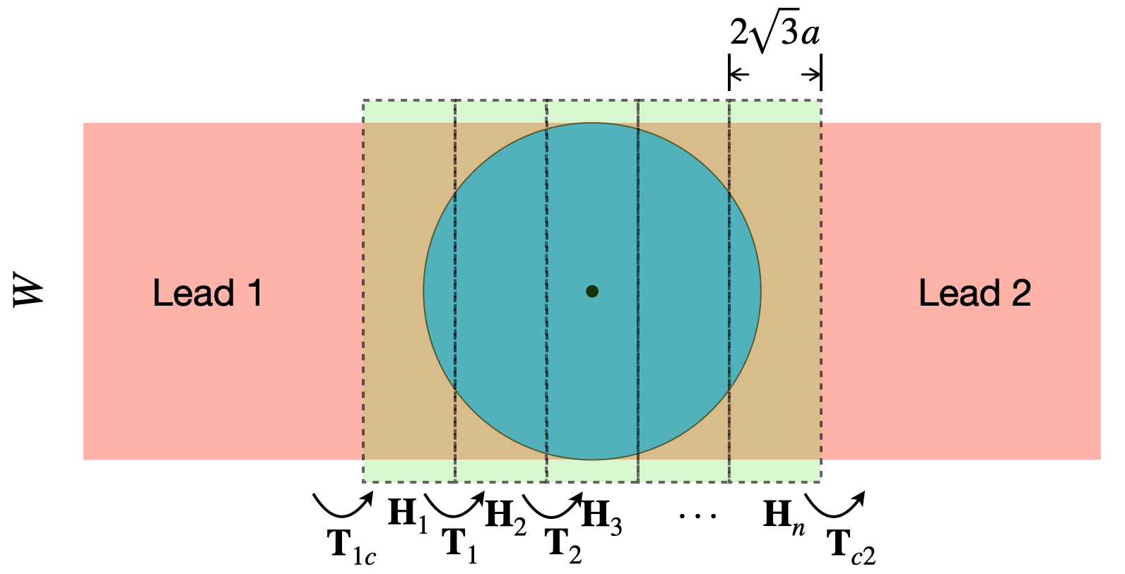
To get the retarded Green’s function of the central region numerically as can be seen in Sec. II, we used an iterative Green’s function method. The detailed algorithm can be seen here: 1) Get all the coordinates of all bottom sites within the central region, the on-site terms and hopping elements of the bottom layer; 2) Get all the coordinates of all bottom layer within the circle (overlapping region); 3) Rotate the coordinates of all bottom sites within the circle to get the coordinates of all top sites; 4) Sort all the top coordinates of the top layer by ascending -coordinate; 5) Divide the central region into several blocks with width (see Fig. 11), so that only the nearest blocks have overlapping hopping integrals. 6) Write down the Hamiltonian of the -th block by calculating the on-site terms and the hopping terms between any two carbon atoms. 7) Write down the hopping matrix between two adjacent blocks and , and the hopping matrices and between the central region and two leads. 8) After, use the iterative Green’s function for the one-dimensional prototype to get the Green’s function .
Appendix B: Periodicity of the transmission coefficient through the TBG region
The peridocity of the transmission through the TBG region without (with) disorder is shown in Fig. 12. The transmission shows a peridocity of as a result of the circular shape of the central TBG region. The transmission also shows a mirror symmetry about [see the black dashed lines in Fig. 12 (a) and (b)] due to the same structure for and , so it is quite resonable to consider only the rotation angle within . Besides the oscillation of the averaged transmission coefficient in Fig. 12(b), the conductance fluctuation also shows oscillations with respect to which minimizes at and peaks at .
Appendix C: Convergence of the transmission coefficients and conductance fluctuation
To test the convergence of the averaged transmission in the main text and the conductance fluctuation calculated from a fixed number of ensemble averages, we first plot the curves with respect to the rotation angle for the disorder average times = 1, 10, 50, 100, 500, 1000 as can be seen in Fig. 14(a). Here we have choose the TBG region in a disc shape with . We find that, for one disorder figuration, the resonant peaks can hardly be distinguished due to the strong fluctuation of the transmission as varying . After making 10 ensemble averages, the first resonant peak can be distinguished. With increasing the averge times, the transmission curves become more smooth, and higher resonant peaks can be clearly distinguished. In Fig. 14(b), we choose the rotaion angle , and give the -dependence of the averaged transmission and conductance fluctuation . Here to show both of them in the same window, we have divided by a factor 20. We see that, the avearged transmission converges quickly after making 100 ensemble averages. However, the conductance fluctuation converges well only after making around 1000 times of averages. To gurantee the ergodicity of our ensemble, we thus choose in all disorder calculations in the main text. However, to get the (or to measure) the resonant peaks in the transmission curves, tens of ensemble averages should be enough, which makes the experimental verification of our results quite feasible.
Appendix D: Avereged transmission coefficients and conductance fluctuation with both-layer disorder
In Fig. 14 we show the calculations on the transport through the TBG device with both-layer disorder. Here the central TBG region is confined within the disc region as we have considered in Sec. III. In Fig. 14 (a, b) we fixed the Fermi energy eV, and show the averged transmission coefficient and the conductance fluctuation as a function of the rotation angle under different both-layer disorder strength . Here the same curve color is used for the same . We see that, for weak disorder eV, the transmission gets an enhancement after due to the decoupling regime of the TBG and shows dependence (fluctuation) with the rotation angle. However, after the disorder strength is increased, the angle dependence(fluctuation) is smeared out and the averaged transmission coefficient shows a constant regardless of the rotation angle, consistent with the calculation in Ref.Namarvar2020Transport. The conductance fluctuation also shows no dependence on the rotation angle. Besides, the transmission gets decreased and approaches zero as increases, which indicates that strong both-layer disorder tends to localize the electrons inside the TBG region, which is quite different from the top-layer disorder case. For the intermediate disorder strength eV, the conductance fluctuation is very close to the universal value of mesoscopic conductance fluctuation , while for strong disorder gets decreased as the transport goes into the localisation regime. These behaviors all indicate that the transport throuth a TBG system is quite similar to the normal 2D systems when both-layer disorder is considered.
To further validate that there is no such geometric resonance in the both-layer disorder case, in Fig. 14(c, d) we show the transport results within a small range of rotation angle () by scanning the disorder strength . We show that, disorder has only two effects on the averaged transmission coefficient : (1) smears out the fluctuation with respect to the rotation angle, and (2) suppresses the transmission. No such resonant peaks are observed in Fig. 14(c, d) around the two moiré resonance angles and .
References
- (1) Y. Cao, V. Fatemi, S. Fang, K. Watanabe, T. Taniguchi, E. Kaxiras, and P. Jarillo-Herrero, Nature 556, 43-50 (2018), Unconventional superconductivity in magic-angle graphene superlattices.
- (2) Y. Cao et al., Nature 556, 80-84 (2018), Correlated insulator behaviour at half-filling in magic-angle graphene superlattices.
- (3) D. Wong, K. P. Nuckolls, M. Oh, B. Lian, Y. Xie, S. Jeon, K. Watanabe, T. Taniguchi, B. A. Bernevig, and A. Yazdani, Nature 582, 198-202, Cascade of electronic transitions in magic-angle twisted bilayer graphene.
- (4) E. Y. Andrei, and A. H. MacDonald, Nat. Mater. 19, 1265-1275 (2020), Graphene bilayers with a twist.
- (5) J. Y. Lee, E. Khalaf, S. Liu, X. Liu, Z. Hao, P. Kim, and A. Vishwanath, Nat. Commu. 10, 5333 (2019), Theory of correlated insulating behaviour and spin-triplet superconductivity in twisted double bilayer graphene.
- (6) L. Balents, C. R. Dean, D. K. Efetov, and A. F. Young, Nat. Phys. 16, 725-733 (2020), Superconductivity and strong correlations in moiré flat bands.
- (7) D. M. Kennes, J. Lischner, and C. Karrasch, Phys. Rev. B 98, 241407(R) (2018), Strong correlations and superconductivity in twisted bilayer graphene.
- (8) F. Wu, and S. Das Sarma, Phys. Rev. B 99, 220507(R) (2019), Identification of superconducting pairiing symmetry in twisted bilayer graphene using in-plane magnetic field and strain.
- (9) X. Gu, C. Chen, J. N. Leaw, E. Laksono, V. M. Pereira, G. Vignale, and S. Adam, Phys. Rev. B 101, 180506(R) (2020), Antiferromagnetism and chiral -wave superconductivity from an effective model for twisted bilayer graphene.
- (10) A. Fischer, L. Klebl, C. Honerkamp, and D. M. Kennes, Phys. Rev. B 103, L041103 (2021), Spin-fluctuation-induced pairing in twisted bilayer graphene.
- (11) C.-C. Liu, L.-D. Zhang, W.-Q. Chen, and F. Yang, Phys. Rev. Lett. 121, 217001 (2018), Chiral Spin Density and Superconductivity in the Magic-Angle-Twisted Bilayer Graphene.
- (12) J. M. B. Lopes dos Santos, N. M. R. Peres, and A. H. Castro Neto, Phys. Rev. B 99, 256802 (2007), Graphene Bilayer with a Twist: Electronic Structure.
- (13) R. Bistritzer, and A. H. MacDonald, Proc. Natl. Acad. Sci. USA 108, 12233 (2011), moiré bands in twisted double-layer graphene.
- (14) J. M. B. Lopes dos Santos, N. M. R. Peres, and A. H. Castro Neto, Phys. Rev. B 86, 155449 (2012), Continuum model of the twisted graphene bilayer.
- (15) E. Suárez Morell, J. D. Correa, P. Vargas, M. Pacheco, and Z. Barticevic, Phys. Rev. B 82, 121407(R) (2010), Flat bands in slightly twisted bilayer graphene: Tight-binding calculations.
- (16) A. L. Sharpe, E. J. Fox, A. W. Barnard, J. Finney, K. Watanabe, T. Taniguchi, M. A. Kastner, and D. Goldhaber-Gordon, Science 365, 605-608 (2019), Emergent ferromagnetism near three-quarters filling in twisted bilayer graphene.
- (17) J.-X. Lin, Y.-H. Zhang, E. Morissette, Z. Wang, S. Liu, D. Rhodes, K. Watanabe, T. Taniguchi, J. Hone, and J. I. A. Li, Science 375, 437-441 (2022), Spin-orbit-driven ferromagnetism at half moiré filling iin magic-angle twisted bilayer graphene.
- (18) Y. Zhang, Z. Hou, Y.-X. Zhao, Z.-H. Guo, Y.-W. Liu, S.-Y. Li, Y.-N. Ren, Q.-F. Sun, and L. He, Phys. Rev. B 102, 081403(R) (2020), Correlation-induced valley splitting and orbital magnetism in a strain-induced zero-energy flatband in twisted bilayer graphene near the magic angle.
- (19) Y. Saito, J. Ge, L. Rademaker, K. Watanabe, T. Taniguchi, D. A. Abanin, and A. F. Young, Nat. Phys. 17, 478-481 (2021), Hofstadter subband ferromagnetism and symmetry-broken Chern insulators in twisted bilayer graphene.
- (20) M. Serlin, C. L. Tschirhart, H. Polshyn, Y. Zhang, J. Zhu, K. Watanabe, T. Taniguchi, L. Balents, and A. F. Young, Science 367, 900-903 (2020), Intrinsic quantized anomalous Hall effect in a moiré heterostructure.
- (21) S. Wu, Z. Zhang, K. Watanabe, T. Taniguchi, and E. Y. Andrei, Nat. Mater. 20, 488-494 (2021), Chern insulators, van Hove singularities and topological flat bands in magic-angle twisted bilayer graphene.
- (22) P. Stepanov et al., Nature 583, 375-378 (2020), Untying the insulating and superconducting orders in magic-angle graphene.
- (23) M. Christos, S. Sachdev, and M. S. Scheurer, Phys. Rev. X 12, 021018 (2022),Correlated Insulators, Semimetals, and Superconductivity in Twisted Trilayer Graphene.
- (24) S. Chen, M. He, Y.-H. Zhang, V. Hsieh, Z. Fei, K. Watanabe, T. Taniguchi, D. H. Cobden, X. Xu, C. R. Dean, and M. Yankowitz, Nat. Phys. 17, 374-380 (2021), Electrically tunable correlated and topological states in twisted monolayer-bilayer graphene.
- (25) Z. Ma, S. Li, Y.-W. Zheng, M.-M. Xiao, H. Jiang, J.-H. Gao, and X.C. Xie, Sci. Bull. 66, 18-22 (2021), Topological flat bands in twisted trilayer graphene.
- (26) Z. Ma, S. Li, M. Lu, D.-H. Xu, J.-H. Gao, and X. C. Xie, Sci. China-Phys. Mech. Astron, 66, 227211 (2023), Doubled moiré flat bands in double-twisted few-layer graphite
- (27) M. Christos, S. Sachdev, and M. S. Scheurer, Phys. Rev. X 12, 021018 (2022), Correlated Insulators, Semimetals, and Superconductivity in Twisted Trilayer Graphene.
- (28) D. Clugru, F. Xie, Z.-D. Song, B. Lian, N. Regnault, and B. A. Bernevig, Phys. Rev. B 103, 195411 (2011), Twisted symmetric trilayer graphene: Single-particle and many-body Hamiltonians and hidden nonlocal symmetries of trilayer moiré systems with and without displacement field .
- (29) F. Xie, N. Regnault, D. Clugru, B. A. Bernevig, and B. Lian, Phys. Rev. B 104, 115167 (2021), Twisted symmetric trilayer graphene. II. Projected Hartree-Fock study.
- (30) Y. Cao, D. Rodan-Legrain, O. Rubies-Bigorda, J. M. Park, K. Watanabe, T. Taniguchi, and P. Jarillo-Herrero, Nature 583, 215-220 (2020), Tunable correlated states and spin-polarized phases in twisted bilayer-bilayer graphene.
- (31) M. Lu, J. Zeng, H. Liu, J.-H. Gao, and X. C. Xie, Phys. Rev. B 103, 195146 (2021), Valley-selective Floquet Chern flat bands in twisted multilayer graphene.
- (32) M. Chen, X. Lin, T. H. Dinh, Z. Zheng, J. Shen, Q. Ma, H. Chen, P. Jarillo-Herrero, and S. Dai, Nat. Mater. 19, 1307-1311 (2020), Configurable phonon polaritons in twisted -MoO3.
- (33) L. Wang et al., Nat. Mater. 19, 861-866 (2020), Correlated electronic phases in twisted bilayer transition metal dichalcogenides.
- (34) D. M. Kennes, M. Claassen, L. Xian, A. Georges, A. J. Millis, J. Hone, C. R. Dean, D. N. Basov, A. N. Pasupathy, and A. Rubio, Nat. Phys. 17, 155-163 (2021), Moiré heterostructures as a condensed-matter quantum simulator.
- (35) Suárez Morell, E. and Vergara, R. and Pacheco, M. and Brey, L. and Chico, Leonor, Phys. Rev. B 89, 205405 (2014), Electronic properties of twisted bilayer nanoribbons.
- (36) E. Suárez Morell and P. Vargas, P. Häberle, A. Hevia, Samuel and L. Chico, Phys. Rev. B 91, 035441 (2015), Edge states of moiré structures in graphite.
- (37) M. Pelc, E. Suárez Morell, L. Brey, and L. Chico, J. Phys. Chem. C 119, 10076–10084 (2015), Electronic Conductance of Twisted Bilayer Nanoribbon Flakes.
- (38) Y. Han, J. Zeng, Y. Ren, X. Dong, W. Ren, and Z. Qiao, Phys. Rev. B 101, 235432 (2020), Mesoscopic electronic transport in twisted bilayer graphene.
- (39) O. F. Namarvar, A. Missaoui, L. Magaud, D. Mayou, and G. Trambly de Laissardire, Phys. Rev. B 101, 245407 (2020), Electronic structure and quantum transport in twisted bilayer graphene with resonant scatterers.
- (40) M. Alvarado, and A. L. Yeyati, Phys. Rev. B 104, 075406 (2021), Transport and spectral properties of magic-angle twisted bilayer graphene junctions based on local orbital models.
- (41) M. Anđelković, L. Covaci, and F. M. Peeters, Phys. Rev. Mater. 2, 034004 (2018), DC conductivity of twisted bilayer graphene: Angle-dependent transport properties and effects of disorder.
- (42) X. Ye, H. Xu, and X. Zhu, New J. Phys. 24, 063029 (2022), Floquet electronic bands and transport in magic-angle bilayer graphene.
- (43) A. S. Ciepielewski, J. Tworzydło, T. Hyart, and A. Lau, Phys. Rev. Res. 4, 043145 (2022), Transport signatures of Van Hove singularities in mesoscopic twisted bilayer graphene.
- (44) G. Sharma, I. Yudhistira, N. Chakraborty, D. Y. H. Ho, M. M. Al Ezzi, M. S. Fuhrer, G. Vignale, and S. Adam, Nat. Commu. 12, 5737 (2021), Carrier transport theory for twisted bilayer graphene in the metallic regime.
- (45) G. Trambly de Laissardire, D. Mayou, and L. Magaud, Nano Lett. 10, 804-808 (2010), Localization of Dirac Electrons in Rotated Graphene Bilayers.
- (46) G. Trambly de Laissardire, D. Mayou, and L. Magaud, Phys. Rev. B 86, 125413 (2012), Numerical studies of confined states in rotated bilayers of graphene.
- (47) V. Nam Do, H. Anh Le, and D. Bercioux, Phys. Rev. B 99, 165127 (2019), Time-evolution of electrons in twisted bilayer graphene.
- (48) G. Li, A. Luican, J. M. B. Lopes dos Santos, A. H. Castro Neto, A. Reina, J. Kong, and E. Y. Andrei, Nat. Phys. 6, 109-113 (2010), Observation of Van Hove singularities in twisted graphene layers.
- (49) A. Luican, G. Li, A. Reina, J. Kong, R. R. Nair, K. S. Novoselov, A. K. Geim, and E. Y. Andrei, Phys. Rev. Lett. 106, 126802 (2011), Single-Layer Behavior and Its Breakdown in Twisted Graphene Layers.
- (50) I. Brihuega, P. Mallet, et al., Phys. Rev. Lett. 109, 196802 (2012), Unraveling the Intrinsic and Robust Nature of van Hove Sigularities in Twisted Bilayer Graphene by Scanning Tunneling Microscopy and Theoretical Analysis.
- (51) L.-J. Yin, J.-B. Qiao, W.-J. Zuo, W.-T. Li, and L. He, Phys. Rev. B 92, 081406(R) (2015), Experimental evidence for non-Abelian gauge potentials in twisted graphene bilayers.
- (52) A. Nimbalkar, and H. Kim, Nano-Micro Lett. 12, 126 (2020), Opportunities and Challenges iin Twisted Bilayer Graphene: A Review.
- (53) A. Luican, G. Li, A. Reina, J. Kong, R. R. Nair, K. S. Novoselov, A. K. Geim, and E. Y. Andrei, Phys. Rev. Lett. 106, 126802 (2011), Single-Layer Behaviour and Its Breakdown in Twisted Graphene Layers.
- (54) I. Brihuega, P. Mallet, H. González-Herrero, G. Trambly de Laissardire, M. M. Ugeda, L. Magaud, J. M. Gómez-Rodríguez, F. Ynduráin, and J.-Y. Veuillen, Phys. Rev. Lett. 109, 196802 (2012), Unraveling the Intrinsic and Robust Nature of van Hove Singularities in Twisted Bilayer Graphene by Scanning Tunneling Microscopy and Theoretical Analysis.
- (55) J. C. Slater and G. F. Koster, Phys. Rev. 94, 1498 (1954).
- (56) M. Mirzakhani, F. M. Peeters, and M. Zarenia, Phys. Rev. B 101, 075413 (2020), Circular quantum dots in twisted bilayer graphene.
- (57) Actually the parameter eV yields a Fermi velocity for the monolayer graphene which fits the experimental data well. In our calculations, we choose eV which shows a small derivation from the experiments but still holds good agreement with the DFT calculations.
- (58) M. P. Lopez Sancho, J. M. Lopez Sancho, J. M. L. Sancho and J Rubio, J. Phys. F: Met. Phys. 15, 851 (1985), Highly convergent schemes for the calculation of bulk and surface Green functions.
- (59) S. Datta, Electronic Transport in Mesoscopic Systems (Cambridge University Press, Cambridge, 1995), pp. 133–136.
- (60) Y. Meir and N. S. Wingreen, Phys. Rev. Lett. 68, 2512 (1992), Landauer Formula for the current through an Interacting Electron Region.
- (61) A.-P. Jauho, N. S. Wingreen, and Y. Meir, Phys. Rev. B 50 5528 (1994), Time-dependent transport in interacting and noninteracting resonant-tunneling systems.
- (62) S. Ryu and Y. Hatsugai, Phys. Rev. Lett. 89, 077002 (2002), Topological Origin of Zero-Energy Edge States in Particle-Hole Symmetric Systems.
- (63) J. M. B. Lopes dos Santos, N. M. R. Peres, and A. H. Castro Neto, Phys. Rev. Lett. 99, 256802 (2007), Graphene Bilayer with a Twist: Electronic Structure.
- (64) J. Berashevich and T. Chakraborty, Phys. Rev. B 84, 033403 (2011), Interlayer repulsion and decoupling effects in stacked turbostratic graphene flakes.
- (65) J. Hass et al., Phys. Rev. Lett. 100, 125504 (2008), Why Multilayer Graphene on 4H-SiC(000) Behaves Like a Single Sheet of Graphene.
- (66) The localization length is calculated by considering a graphene nanoribbon with a rectangular disordered region with the Green’s function method.
- (67) We take the function as an example. The positions of the peaks locate at which yields and moves leftward as increases. We ascribe the moving of the first resonant peak to the same reason here.
- (68) The higher Fermi level crosses more transmission channels from the leads so that the density of states within the TBG region beome more, and as a result, the resonant transmission mediated by the quantum dot structure formed naturally within the TBG moiré pattern becomes prominent.
- (69) P. Moles, F. Domínguez-Adame, and L. Chico, arXiv:2307.06819v1 (2023), Impact of vacancies on twisted bilayer graphene quantum point contacts.