Sensitivity of Space-based Gravitational-Wave Interferometers to Ultralight Bosonic Fields and Dark Matter
Abstract
Ultralight bosonic fields (ULBFs) are predicted by various theories beyond the standard model of particle physics and are viable candidates of cold dark matter. There have been increasing interests to search for the ULBFs in physical and astronomical experiments. In this paper, we investigate the sensitivity of several planned space-based gravitational-wave interferometers to ultralight scalar and vector fields. Using time-delay interferometry (TDI) to suppress the overwhelming laser frequency noise, we derive the averaged transfer functions of different TDI combinations to scalar and vector fields, and estimate the impacts of bosonic field’s velocities. We obtain the sensitivity curves for LISA, Taiji and TianQin, and explore their projected constraints on the couplings between ULBFs and standard model particles, illustrating with the ULBFs as dark matter.
Keywords:
Dark Matter, Ultralight fields, Gravitational wave, Time-Delay InterferometryI INTRODUCTION
On September 14, 2015 the LIGO detectors detected the first gravitational-wave signal generated from a binary black hole merger Abbott et al. 2016, which opens the era of gravitational astronomy Sathyaprakash and Schutz 2009. Since then, over ninety gravitational wave events have been detected, which not only brings us many valuable information about the Universe but also shows the incredible ability of interferometry detector. Precision interferometers can measure the relative displacements of two mirrors separated several kilometers apart at subatomic level. Besides gravitational waves, other physical processes may also generate the relative displacement of mirrors (test masses). Thus interferometer gravitational-wave detectors can also be used to search for the signals of those physical processes.
This idea has been recently explored, for example in Pierce et al. 2018; Morisaki and Suyama 2019; Michimura et al. 2020a; Morisaki et al. 2021, which propose to use interferometers to search for ultralight dark matter (ULDM) Kawasaki and Nakayama 2013; Marsh 2016; Hui et al. 2017; Hui 2021; Ferreira 2021. Since ULDM particles are very light, typically below eV, there are numerous ULDM particles in a de Broglie volume (for eV, the average number of particles ). The occupancy number is so large that the quantum fluctuations are negligible and the set of ULDM particles can be well described by classical bosonic fields that oscillate at the Compton frequency. When ULDM is coupled to the SM particles, its oscillation will effectively exert a periodical force on the test masses and induce spatial displacements of them, which may end up with detectable signal in the interferometer. Searching for the ULDM signals in the data of LIGO Abbott et al. 2022; Guo et al. 2019; Fukusumi et al. 2023 and LISA Pathfinder Miller and Mendes 2023 has been conducted recently. Although reporting null results, these works show that high precision interferometers can put stringent constraints on the coupling constants close to or even comparable with constraints given by equivalence principle tests and fifth-force experiments Adelberger et al. 2003a; Schlamminger et al. 2008a; Touboul et al. 2022a; Graham et al. 2016a; Grote and Stadnik 2019.
In the above works, it was assumed that the ultralight bosonic fields serve as dark matter, therefore the amplitudes of fields are determined by the local dark matter density and the frequency dispersion of fields follows from the velocity dispersion of DM. However, besides DM, ULBFs are widely predicted in physical and cosmological theories for various motivations, and have been actively investigated on different forms Peccei and Quinn 1977; Wilczek 1978; Weinberg 1978; Preskill et al. 1983; Abbott and Sikivie 1983; Dine and Fischler 1983; Nelson and Scholtz 2011; Graham et al. 2016b; Ema et al. 2019; Ahmed et al. 2020; Agrawal et al. 2020; Tang and Wu 2020; Kitajima and Nakayama 2023; Kolb and Long 2021; An et al. 2021; Moroi and Yin 2021; Liang et al. 2023; Sun et al. 2022; An et al. 2023; Luu et al. 2023; Liu et al. 2023; An et al. 2023; Chen et al. 2020; Tang et al. 2023; Grote and Stadnik 2019; Xia et al. 2021; Fayet 1980; Fayet 1989; Fayet 1990; Fayet 2018; Wu et al. 2023 since many possible field configurations could exist. In this work, we take a systematic approach and drop the assumption that ULBF makes up the local DM, which implies the amplitude of field and the velocity of filed are generic. We investigate the ability of interferometers to constrain the combinations of coupling constants and field amplitudes in the more general setup and illustrate with the DM case. In the prospects of the increasing sensitivity of operating interferometer detectors Aasi et al. 2015; Acernese et al. 2015 and the next generation ground-based detectors like Cosmic Explorer Evans et al. 2021, Einstein Telescope Punturo et al. 2010 and space-based detectors like LISA Amaro-Seoane et al. 2017, Taiji Hu and Wu 2017 and TianQin Luo et al. 2016, we show it is possible to detect weaker ULBF signals or put more stringent constraints on the coupling constants and amplitudes of the fields in the null case by space-based detectors.
In this work, we focus on two kinds of ULBF, scalar and vector, in the mass range eV, which corresponds to the sensitive band of space-based gravitational-wave interferometers. We investigate their potential to detect ULBF signals by calculating response functions and sensitivity curves of several main time-delay interferometry combinations Estabrook et al. 2000; Tinto and Dhurandhar 2005, such as Michelson , Sagnac , fully symmetric Sagnac and optimal channel . Our results show future space-based detectors can provide a better probe in some parameter regions.
This paper is organized as follows. In Sec. II, we present the scalar and vector models and explain how these ultralight bosonic fields affect the motion of test masses. One of the key result is the single-link transfer function of interferometer to the bosonic fields. In Sec. III, we construct the sky and polarization averaged transfer functions of different TDI combinations from the single-link transfer function and discuss their asymptotic behaviors in the long wavelength limit and contrast them with the case for gravitational wave. In particular, we show the effects of field velocity on the transfer function. Then we calculate the sensitivity curves of Taiji, LISA and TianQin to ULBF in Sec. IV and illustrate with dark matter case in Sec. V. Finally, we give our conclusion in Sec. VI.
In this paper, we use natural units () unless explicitly stated otherwise.
II Formalism and Conventions
In this section, we introduce our conventions for scalar and vector fields, and their ways of interacting with ordinary matter. We obtain the equation of motion for the test masses through the action of the system and give the spatial displacements of the test masses, which is essential for subsequent discussions. The physical picture is that the spatial shifts affect the optical lengths of laser beams, which induces the phase difference or equivalently the frequency shift that will be detected by the phasemeters.
II.1 Scalar field
Ultralight scalar fields for spin-0 particles appear in many popular physical and cosmological theories, such as axions, dark matter, dilaton and dark energy models. Here, we do not specify the exact model but only present a general formalism. We denote as a scalar field which linearly couples to SM particle mass terms. Then the effective Lagrangian of the system at the low-energy limit is given by
| (1) |
where is the Lagrangian of the scalar field and usually can be expressed by , is the Lagrangian of the Standard Model and for the interaction between the scalar field and the ordinary matter. The details of the interaction will be presented in Sec. V. At the moment, we can work in the low-energy limit and treat the test mass as a function of and the action of the test mass is given by Morisaki and Suyama 2019
| (2) |
The effective scalar-matter coupling is encoded in the mass and defined by
| (3) |
where is the inverse of the Planck mass and used here for a reference scale.
Without loss of generality, we use a monochromatic plane wave to describe the scalar field as a transient source:
| (4) |
where is the amplitude of the wave, the de Broglie angular frequency, the momentum vector of the scalar field, and an initial phase whose exact value does not affect our discussion and can be set to zero. When the scalar field is referred as DM in our galaxy, it has a velocity dispersion, , which implies that the wave is non-relativistic with and . We can also extend the case to the relativistic condition, the details will be discussed later.
Using the Euler-Lagrangian equation and neglecting the subdominant term related to the velocity of test mass, we get the additional acceleration and displacement induced by the oscillation of scalar field:
| (5) |
We can integrate the above equations twice and obtain the spatial displacement,
| (6) |
where is the unit vector of and .
II.2 Vector field
Ultralight vector fields for spin-1 particles are also well motivated theoretically, such as very light scaling gauge field for DM candidate Wu 2016; Wu 2018; Wu 2023; Tang and Wu 2020; Wang et al. 2022. Vector field can directly couple with the baryon number (B) or baryon minus lepton number (B-L) and it will exert an additional force on the test masses, which leads to the periodic displacements of test masses.
The Lagrangian of the massive vector field coupled with B or B-L current is given by
| (7) |
where , is the vector field and is the mass of vector field. Here we normalize the coupling strength of the vector field in terms of the electromagnetic coupling constant and denote as the ratio Michimura et al. 2020b.
The spatial components of are described by
| (8) |
where is the unit polarization vector which is parallel to . Here we ignore since it is much smaller than under Lorentz gauge in the non-relativistic limit. A object carrying B or B-L charge can be accelerated by the electric-like field generated by the vector field. The acceleration acting on the test mass can be written as Michimura et al. 2020b; Pierce et al. 2018
| (9) |
where is the mass of the jth test mass. is the total baryon number if the vector field is a gauge field, and only counts the neutrons in the test masses if it is associated with gauge symmetry. We can integrate Eq. (9) twice and obtain the spatial displacement of the test mass:
| (10) |
where . Comparing it with the scalar case, Eq. (6), we can find that the difference is that in Eq. (6) is replaced by in Eq. (10). Therefore, both transverse and longitudinal modes contribute.
III Transfer function
In this section, we discuss how the displacement signals induced by ULBFs manifest in the physical measurements. We establish the necessary formalism to describe the transfer function, including the detector response of a single link and time-delay interferometry.
III.1 The detector frame
The detector coordinate system is chosen such that the three arms of the triangle detector keep fixed in the plane with the first spacecraft (SC) located at , the second located at and the third located at , where is the opening angle between the two arms of the interferometer and is the static length of the arm. The wave propagation direction is
and two orthogonal vectors , can be chosen as the polarization basis vectors. The details of coordinate system is shown in Fig. 1.

III.2 Transfer functions of a single link
Now we can calculate the frequency shift of laser caused by the motion of test masses and we will derive the one-link transfer functions in this section, which are essential for the discussions of transfer functions of TDI combinations.
Since the test masses will oscillate under the influence of ULBF, the time that the laser need to propagate from sender SC () to receiver SC () will vary with time,
| (11) |
where is the static length of the arm in the absence of ULBF and is perturbation of one-way time due to the ULBF oscillation,
| (12) |
where is the unit vector pointing from to and is the arrival time of laser recorded by the receiver. The laser phase received at equals the laser phase sent at ,
| (13) |
where is the fiducial frequency of laser. The instantaneous frequency measured on the receiving spacecraft is related to through
| (14) |
Thus, the relative frequency shift or fractional frequency fluctuation is
| (15) |
Combining Eq. (12) and Eq. (15), one-way Doppler shift can be expressed as
| (16) |
where and is the geometric factor given by
| (17) |
where we have included the response for gravitational wave for comparison, is the polarization tensor and is the polarization angle for gravitational wave. As can be seen from Eq. (16), with the definition of , the one-way Doppler signals of scalar fields, vector fields and gravitational waves can be written in a concise and unified form. Follow from it, the TDI combinations, which are composed of time-shifted one-way Doppler signals, also have identical forms for scalar fields, vector fields and gravitational waves.
If the Doppler shift is recorded within a period of time , the corresponding Fourier transform of becomes
| (18) |
Putting Eq.(18) in Eq.(16), we obtain
| (19) |
where and is the Fourier amplitude of . Then we can extract the Fourier transformation of from Eq. (19):
| (20) |
Here we have neglected the time-dependence of in , which follows the convention in the gravitational-wave literature and is compensated by the average of different directions.
The sky and polarization averaged transfer function is defined as
| (21) |
where the overline denotes the average over all propagation directions and polarization angles. Explicitly, for scalar field, we have
| (22) |
For vector field, we have
| (23) |
where is the two-dimensional spherical coordinates of . For gravitational waves, we have
| (24) |
We define the integration operations for later convenience,
| (25) | ||||
| (26) | ||||
| (27) |
III.3 Transfer functions of TDI combinations
As can be seen from Eq. (19), the signal in one-link is a modulated Doppler shift with amplitude proportional to whose typical magnitudes for astrophysical sources are of order . However, the current baseline for stabilized laser has a power spectral density as high as or in relative frequency fluctuation for laser with wavelength nm. Thus the laser frequency noise dominates in the one-link signals. In ground-based interferometer detectors, we do not need to worry about the laser noise in one link signals, since it will be suppressed significantly when the beams are combined at the photon detector due to the equal length of the two arms of Michelson interferometer. However, for space-borne interferometer detectors, the distances between pairs of spacecrafts evolve with time and can not keep equal with each other. Therefore the laser noise will not be cancelled by the simple Michelson configuration. To tackle this problem, TDI is used Estabrook et al. 2000; Tinto and Dhurandhar 2021 for data postprocessing. The essential idea is to use the data of six links to synthesize virtual interferometric configurations that have almost equal light paths. It has been shown that the magnitude of residual laser noise in the synthesized data meets the requirement of sensitivity of gravitational waves detection.
In this section, we discuss the response of the TDI-1.5 configurations which apply to a non-equal arms, rigid but rotating triangle constellation. For the sake of simplicity and physical intuition, we focus on the equilateral-triangle configuration and ignore the motion of spacecrafts, since the final sensitivity curves do not depend on which generation TDI is. We perform the sky and polarization average of the transfer functions in both semi-analytical numerical integration and Monte Carlo integration with source positions per frequency bin as a cross check of our results.
We follow the convention used in Otto 2015 for TDI discussions. The opposite arm of spacecraft is denoted by (counter-clockwise) and (clockwise), respectively. is the shorthand for time-delayed series.
III.3.1 Michelson interferometry
We start with equal-arm Michelson configuration , which can be synthesized from the four one-link signals,
| (28) |
And in the static and equal armlength case, it reduces to
| (29) |
The corresponding Fourier transform is given by
| (30) |
where . After substituting Eq. (30) into Eqs. (22) and (23), the sky and polarization averaged transfer functions , of Michelson configuration can be expressed as
| (31) | |||||
| (32) |
and the expressions of and can be found in Appendix A.
III.3.2 Michelson combinations
The Michelson combination in TDI-1.5 is given by
| (33) |
For the static and equal armlength case,
| (34) | |||||
Michelson and combinations can be obtained by cyclic permutation of the indices . The Fourier transform is related to through
| (35) |
This relation is a general consequence of the similarity between structures of Eq. (29) and Eq. (34). Using Eq. (35), the averaged transfer functions , of combination can be expressed as
| (36) | |||||
| (37) |
After sky and polarization averaged, the transfer functions of , combinations are the same as Eq. (36, 37).
In the first plot in Fig. 2, we show the transfer functions for Michelson combinations. We can see that in the low frequency range Hz which corresponds to ( is the velocity of the field), . However, when Hz, namely, , . This is accord with the asymptotic behavior of GWs, . Thus, is the critical frequency at which the asymptotic behaviors change. This effect is due to the velocity of the scalar and vector fields.
In the long wavelength limit, we can perform the sky average analytically and Eq. (36) reduces to
| (38) |
For non-relativistic fields, the field velocity is a small quantity. The first term is dominant when and the second term become more important when .
III.3.3 Sagnac combinations:
The six-link Sagnac combinations , , are the generators of the space of laser noise free combinations. The expression of combination is
| (39) |
which in the static and equal armlength case reduces to
| (40) |
, can be obtained by cyclic permutation of the indices (1,2,3). The transfer function , of combination can be expressed as
| (41) | |||||
| (42) |
where the detail expressions of and are presented in the Appendix. The averaged transfer functions of and are the same as Eq. (41, 42).
The asymptotic behaviors of Sagnac combinations in the low frequency region are the same as the behaviors of Michelson combinations. In Fig. 2, we can see that in the low frequency range Hz, . However, when Hz, , same as the asymptotic behavior of GWs, .
III.3.4 Fully symmetric Sagnac combination:
Another important combination is the fully symmetric combination , given by
| (43) |
For the static and equal armlength case, we have
| (44) |
The averaged transfer functions of combination can be expressed as
| (45) | |||||
| (46) |
The expressions of and can be found in the Appendix.
From Fig. 2, it is clear to see that in the low frequency limit Hz, , and . It is worth noting that the asymptotic behaviors of scalar field and GWs are true only when the detector array is equilateral triangle. If the array has unequal armlength, then will be proportional to in the low frequency limit. At frequencies equal integers of the inverse of light travel time, the response of the detector is subtracted to zero due to the overall factor in Eq. (45, 46).
There are two interesting points here. The first is that is not sensitive to the field velocity in the sense that there is only one asymptotic behavior of transfer function in the low frequency region and no critical frequency compared to Michelson combinations. The second is that the unexpected asymptotic behavior of vector field which is proportional to rather than .
To understand these phenomena, we derive the approximate expression of in the long wavelength limit,
| (47) |
where . It shows the field velocity and appear as a combination in Eq. (47). Furthermore, for scalar field and the longitudinal polarization of vector field, , and the coefficient of cancels due to the geometrical relation . Thus, the leading-order contribution is . However, for the transverse polarization of vector field, this cancellation doesn’t happen and the leading order is . We further decompose the into for transverse mode and for longitudinal mode. Following Eq. (47), we find that and in the low frequency limit in the equal armlength case. Thus, transverse polarization dominates the asymptotic behavior of in the low frequency region.
Besides serving as the noise monitor, combination may have another advantage. If a monochromatic signal is detected, we need to distinguish ULBFs from galactic white dwarf binaries that can also produce nearly monochromatic gravitational waves. We can utilize the difference of transfer functions between and combinations for ULBFs and GWs. Given a ULBF and a white dwarf binary which produce the same magnitude signals in the combination, the signal of ULBF in combination may be overwhelmed by the noise due to the smaller value of transfer function while the signal of GWs in combination will survive. This suggests that the ratios of signal-to-noise in two combinations are different in two cases.
III.3.5 Optimal combinations
The Michelson combinations , and can be further assembled into three optimal combinations, and Prince et al. 2002,
| (48) |
The expressions of the averaged transfer functions of , and can be found in the Appendix. As can be seen in Fig. 2, , in Hz and , when Hz (the values of and are equal across the band). In the equal armlength case, , and in the low frequency region. The different behavior of vector field is also due to the similar reason that the transverse polarization () dominates the longitudinal polarization () as explained in .
III.4 Comparison of transfer functions of ULBFs with GWs
In the previous calculations, we adopted the assumption that , which results in a different shape of transfer function compared to the case of gravitational waves, including the oscillating behavior in the high-frequency region and the trends in low-frequency region. Now we give a physical explanation for the difference.
In previous sections, we obtain the displacement caused by bosonic fields in the non-relativistic case. In fact, we can directly apply the displacement formula of the detector under the influence of an ultralight scalar field to the relativistic case. This is because in the calculations we did not impose any assumption on the velocity of scalar field. Thus, the displacement formula derived earlier can still be used. But one should notice that, if the scalar field is relativistic, the approximation of is no longer applicable and should be replaced with .
For simplicity, we will first compare the single-link responses and then discuss the transfer functions of TDI combinations.
The Fourier amplitude of the single-link signal is given by Eq.(20) and the corresponding transfer function is
| (49) |
For scalar field, , different from for gravitational waves. Without lose of generality, we use the arm to calculate the single-link response function in the case of scalar field and gravitational waves. The result is shown in Fig. 3. In the low-frequency region, the transfer function of the scalar field differs from that of the gravitational waves by a velocity-dependent factor. The leading-order term of the ratio in low frequency approximation is
| (50) |
In the high frequency region, the velocity of the field affects the oscillation behavior. To be more specific, as increases, the second term related to the propagation direction in the trigonometric function in Eq. (49) becomes non-negligible, which will lead to the change of the oscillation period. At the same time, averaging the entire sky will result in a decrease in the oscillation amplitude, since while cancellation appear in some directions at a fixed frequency, it will not happen in other directions.
Now we consider the TDI combinations. The differences between transfer functions are similar to the single-link case. We illustrate with the transfer function of combination with respect to the frequency and the velocity in Fig. 4.
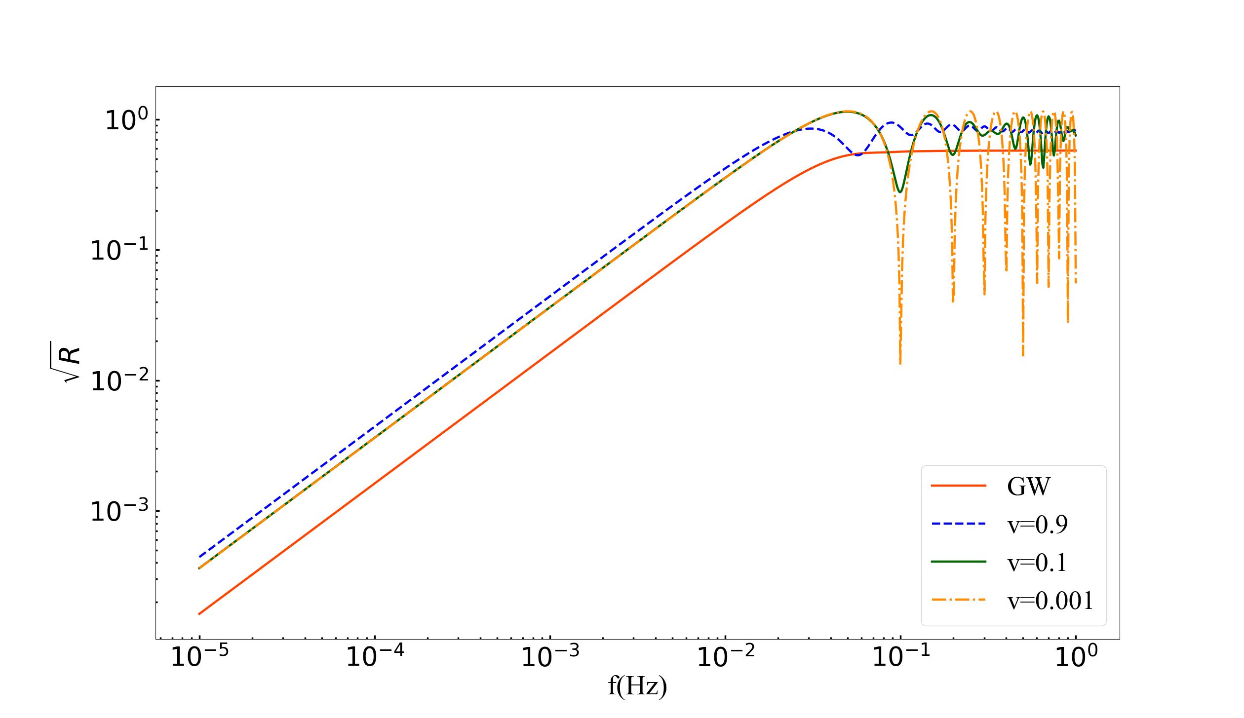

From the result, we find that with the increasing velocity, the overall trend of the transfer function and the oscillation behavior of the high frequency part are closer to the behavior of gravitational wave. When the velocity of the scalar field approaches the speed of light, there is only a slight difference between the two cases, which is caused by .
IV Sensitivity curves
The sensitivity of individual TDI combination is defined by Babak et al. 2021
| (51) |
where is the one-sided noise power spectral density (PSD) of combination and is the averaged transfer function of .
After suppression of the laser noise below the requirement, the two secondary noises determine the performance of detector. The first one is related to optical metrology system (oms) noise, which dominates at high frequency. The second one is the test mass acceleration noise (acc) that dominates at low frequency. The magnitudes of oms and acc noises for LISA Amaro-Seoane et al. 2017, Taiji Hu and Wu 2017, TianQin Luo et al. 2016 are
| (52) | |||||
| (53) |
where we use the following noise parameters,
| LISA | |||||
| Taiji | |||||
| TianQin | (54) |
We adopt the same frequency dependent factors in Eqs. (52, 53) for a straightforward comparison of the sensitivity of the three detectors.
Since we perform TDI algorithm with the one-link output, the remaining noises in the output of TDI are also the linear combinations of the time shifted noises in one-link output. We derived the PSD for the TDI-1.5 combinations (PSD of other TDI combinations can be found in Appendix B):
| (55) | |||||
| (56) | |||||
| (57) |
With the averaged transfer function and PSD of the TDI combinations at hand, we can calculate sensitivity curves. In Fig. 5, we plot the sensitivity of Michelson combination of the three detectors to the ULBFs.
The optimal sensitivity is defined by
| (58) |
In Fig. 6 we compare the optimal sensitivity with combination sensitivity for Taiji. For gravitational waves, the ratio between and oscillates with an average value in the high frequency part. However, for scalar and vector fields, the ratio oscillates above in the high frequency part. This difference comes from the relative magnitudes between , and in the high frequency band in the two cases. As shown in Fig. 6, for gravitational waves, although in the long wavelength region the sensitivity of and are much better than , will have comparable sensitivity in the high frequency region. For scalar and vector fields, has much worse sensitivity than and across the whole band, thus will not contribute to significantly.
V Illustrations of Constraints on Dark Matter


In this section, we estimate the future constraints on dark matter (DM) models based on the results in the previous sections.
For scalar field, we consider the following interactions as an illustration Damour and Donoghue 2010; Piazza and Pospelov 2010,
| (59) |
where ; are the gluon field strength tensors; is the gauge coupling; and refers to the QCD beta functions; are the anomalous dimensions of the and quarks; is the couplings to the gluonic field term, and and are the couplings to the quark mass terms. It is more convenient to define
| (60) |
Since the nucleon mass is mostly determined by the QCD energy scale, in Eq. (3) is approximately given by
| (61) |
Considering that scalar or vector fields make up all the dark matter components, we have
| (62) |
where GeVcm3 is an estimate of the local density of DM, and is the velocity dispersion of the dark matter in our Galaxy.
The minimum detectable Fourier amplitude is
| (63) |
where refers to the duration of observation time. We assume that the duration is shorter than the coherence time of the field s, so that the approximation of monochromatic plane wave is satisfied. Moreover, local DM should be treated as a superposition of plane waves with different propagation directions and velocities and a factor has been found in the estimation of laboratory experimental searches Centers et al. 2021. Here, we just use the monochromatic plane wave for illustration and more dedicated study on the stochastic DM will be conducted in the coming work.
Using the standard sensitivity curve of combination, we express the constrain with respect to ,
| (64) |
The constraint curves of coupling constant given by space-based detectors are plotted in Fig. 7, assuming and . Relevant constraints from other experiments, including the fifth-force experiment Adelberger et al. 2003b and the tests of equivalence principle (EP tests) Wagner et al. 2012; Touboul et al. 2017, are also shown. All detectors will provide more stringent constraints than the fifth-force experiments in some parameter space. The constraint given by TianQin can reach , which approaches the lower limit of the fifth-force experiment. Compared to the EP tests, LISA and Taiji can reach and at eV and eV, respectively, and the improvement factors are 6 and 16, respectively. In the low mass region, Eq. (64) has the approximate expression, , i.e. the sensitivity is inversely proportional to the square of the arm length. Therefore, LISA and Taiji will have much better sensitivity of compared to TianQin at low-mass region.
Similarly, the Fourier amplitude of the vector field is given by
| (65) |
Using the sensitivity curve of combination for vector fields, we have
| (66) |
For a gauge boson, is almost identical among different materials, where is the mass number, is the atomic mass in atomic units and refers to the mass of neutron. But for a gauge boson, , and the neutron ratio would be different between materials. Here we use for a gauge boson and for a gauge boson.
The constraints on coupling constants and given by space-based detectors are plotted in Fig. 8. As a comparison, the results of Eöt-Wash experiment and MICROSCOPE are also shown 11 1 The results of MICROSCOPE shown here are from the first results of the experiment Touboul et al. 2017. According to the latest results Touboul et al. 2022b, the constraints would be improved by a factor of . Private communication with P. Fayet.. Compared to EP test, gravitational-wave detectors can provide better constraints on coupling constants and in some parameter space. For , the best constraints projected by LISA, Taiji and TianQin in the sensitive range are improved by , and respectively. And for , the improvement factors are , and . As we can see, LISA and Taiji will have much better sensitivity of and compared to TianQin at low-mass region because of the longer arm length.
VI Summary and Conclusions
Ultralight bosonic fields (ULBFs) are well-motivated and predicted in many physical and cosmological theories. When having tiny couplings to standard model particles, they may be probed by precision gravitational-wave interferometers. We investigate the sensitivity of space-based gravitational-waves detectors to ULBFs systematically. We obtain the sky and polarization averaged transfer functions of various time-delay interferometry (TDI) combinations and discuss their asymptotic behaviors in the long wavelength region. We find that the velocity of field will affect the behaviors of transfer function, more significantly at high mass region. For TDI combinations like Michelson, Sagnac and optimal , , there exists a critical frequency determined by the field velocity and arm length , below which transfer functions and are similar to gravitational waves; however, for Hz, are proportional to . For combinations like and , although there is no critical frequency, the magnitudes of transfer functions for scalar and vector fields are much smaller than that for gravitational waves. The physical reason is that, for the same frequency these non-relativistic waves will have much longer wavelength compared to gravitational waves, and and are not sensitive to the common displacements of the spacecrafts due to their symmetric structure.
A direct application of our result is to identify ULBFs as dark matter (DM). We estimate the ability of detectors to search DM by calculating the sensitivity curves of future space-based interferometers, which can improve the current limits by several orders of magnitude, see Figs. 7 and 8. We should note that it is more realistic and appropriate to treat the local DM as a stochastic waves background rather than monochromatic waves Centers et al. 2021; Derevianko 2018; Foster et al. 2018; Kim 2023. Therefore, the precise sensitivity of detectors to the local DM need a more dedicated study. We will leave the stochastic effect of the fields to future work.
acknowledgement
Y.T is supported by National Key Research and Development Program of China (Grant No.2021YFC2201901), and National Natural Science Foundation of China under Grants No.12147103 and 11851302. Y.L.W. is supported by the National Key Research and Development Program of China under Grant No.2020YFC2201501, and NSFC under Grants No. 11690022, No. 11747601, No. 12147103, and the Strategic Priority Research Program of the Chinese Academy of Sciences under Grant No. XDB23030100.
Appendix A Analytic expressions of the transfer functions
Explicit forms of some functions appearing in the transfer functions of Michelson and Sagnac combinations are listed below.
The transfer function , for various optimal combinations can be expressed as
| (67) | |||||
| (68) |
| (69) | |||||
| (70) |
| (71) | |||||
| (72) |
where we have defined the following functions,
Appendix B Power spectral density of TDI combinations
The noise power spectral density of different TDI channels are calculated and summarized below. Michelson X, Y, Z:
| (73) |
Fully symmetric Sagnac :
| (74) |
Sagnac , , :
| (75) |
Beacon P, Q, R:
| (76) |
Monitor E, F, G:
| (77) |
Relay U, V, W:
| (78) | |||||
Optimal A, E, T:
| (79) | |||||
| (80) |
References
- Abbott et al. (2016) B. P. Abbott et al. (LIGO Scientific, Virgo), Observation of Gravitational Waves from a Binary Black Hole Merger, Phys. Rev. Lett. 116, 061102 (2016), arXiv:1602.03837 [gr-qc] .
- Sathyaprakash and Schutz (2009) B. S. Sathyaprakash and B. F. Schutz, Physics, Astrophysics and Cosmology with Gravitational Waves, Living Rev. Rel. 12, 2 (2009), arXiv:0903.0338 [gr-qc] .
- Pierce et al. (2018) A. Pierce, K. Riles, and Y. Zhao, Searching for dark photon dark matter with gravitational-wave detectors, Phys. Rev. Lett. 121, 061102 (2018).
- Morisaki and Suyama (2019) S. Morisaki and T. Suyama, Detectability of ultralight scalar field dark matter with gravitational-wave detectors, Phys. Rev. D 100, 123512 (2019).
- Michimura et al. (2020a) Y. Michimura, T. Fujita, S. Morisaki, H. Nakatsuka, and I. Obata, Ultralight vector dark matter search with auxiliary length channels of gravitational wave detectors, Phys. Rev. D 102, 102001 (2020a), arXiv:2008.02482 [hep-ph] .
- Morisaki et al. (2021) S. Morisaki, T. Fujita, Y. Michimura, H. Nakatsuka, and I. Obata, Improved sensitivity of interferometric gravitational wave detectors to ultralight vector dark matter from the finite light-traveling time, Phys. Rev. D 103, L051702 (2021), arXiv:2011.03589 [hep-ph] .
- Kawasaki and Nakayama (2013) M. Kawasaki and K. Nakayama, Axions: Theory and Cosmological Role, Ann. Rev. Nucl. Part. Sci. 63, 69 (2013), arXiv:1301.1123 [hep-ph] .
- Marsh (2016) D. J. E. Marsh, Axion Cosmology, Phys. Rept. 643, 1 (2016), arXiv:1510.07633 [astro-ph.CO] .
- Hui et al. (2017) L. Hui, J. P. Ostriker, S. Tremaine, and E. Witten, Ultralight scalars as cosmological dark matter, Phys. Rev. D 95, 043541 (2017), arXiv:1610.08297 [astro-ph.CO] .
- Hui (2021) L. Hui, Wave Dark Matter, Ann. Rev. Astron. Astrophys. 59, 247 (2021), arXiv:2101.11735 [astro-ph.CO] .
- Ferreira (2021) E. G. M. Ferreira, Ultra-light dark matter, Astron. Astrophys. Rev. 29, 7 (2021), arXiv:2005.03254 [astro-ph.CO] .
- Abbott et al. (2022) R. Abbott et al. (LIGO Scientific, KAGRA, Virgo), Constraints on dark photon dark matter using data from LIGO’s and Virgo’s third observing run, Phys. Rev. D 105, 063030 (2022), arXiv:2105.13085 [astro-ph.CO] .
- Guo et al. (2019) H.-K. Guo, K. Riles, F.-W. Yang, and Y. Zhao, Searching for Dark Photon Dark Matter in LIGO O1 Data, Commun. Phys. 2, 155 (2019), arXiv:1905.04316 [hep-ph] .
- Fukusumi et al. (2023) K. Fukusumi, S. Morisaki, and T. Suyama, Upper limit on scalar field dark matter from LIGO-Virgo third observation run, (2023), arXiv:2303.13088 [hep-ph] .
- Miller and Mendes (2023) A. L. Miller and L. Mendes, First search for ultralight dark matter with a space-based gravitational-wave antenna: Lisa pathfinder, Phys. Rev. D 107, 063015 (2023).
- Adelberger et al. (2003a) E. G. Adelberger, B. R. Heckel, and A. E. Nelson, Tests of the gravitational inverse square law, Ann. Rev. Nucl. Part. Sci. 53, 77 (2003a), arXiv:hep-ph/0307284 .
- Schlamminger et al. (2008a) S. Schlamminger, K. Y. Choi, T. A. Wagner, J. H. Gundlach, and E. G. Adelberger, Test of the equivalence principle using a rotating torsion balance, Phys. Rev. Lett. 100, 041101 (2008a), arXiv:0712.0607 [gr-qc] .
- Touboul et al. (2022a) P. Touboul et al. (MICROSCOPE), MICROSCOPE Mission: Final Results of the Test of the Equivalence Principle, Phys. Rev. Lett. 129, 121102 (2022a), arXiv:2209.15487 [gr-qc] .
- Graham et al. (2016a) P. W. Graham, D. E. Kaplan, J. Mardon, S. Rajendran, and W. A. Terrano, Dark Matter Direct Detection with Accelerometers, Phys. Rev. D 93, 075029 (2016a), arXiv:1512.06165 [hep-ph] .
- Grote and Stadnik (2019) H. Grote and Y. V. Stadnik, Novel signatures of dark matter in laser-interferometric gravitational-wave detectors, Phys. Rev. Res. 1, 033187 (2019), arXiv:1906.06193 [astro-ph.IM] .
- Peccei and Quinn (1977) R. D. Peccei and H. R. Quinn, conservation in the presence of pseudoparticles, Phys. Rev. Lett. 38, 1440 (1977).
- Wilczek (1978) F. Wilczek, Problem of strong and invariance in the presence of instantons, Phys. Rev. Lett. 40, 279 (1978).
- Weinberg (1978) S. Weinberg, A new light boson?, Phys. Rev. Lett. 40, 223 (1978).
- Preskill et al. (1983) J. Preskill, M. B. Wise, and F. Wilczek, Cosmology of the Invisible Axion, Phys. Lett. B 120, 127 (1983).
- Abbott and Sikivie (1983) L. F. Abbott and P. Sikivie, A Cosmological Bound on the Invisible Axion, Phys. Lett. B 120, 133 (1983).
- Dine and Fischler (1983) M. Dine and W. Fischler, The Not So Harmless Axion, Phys. Lett. B 120, 137 (1983).
- Nelson and Scholtz (2011) A. E. Nelson and J. Scholtz, Dark Light, Dark Matter and the Misalignment Mechanism, Phys. Rev. D 84, 103501 (2011), arXiv:1105.2812 [hep-ph] .
- Graham et al. (2016b) P. W. Graham, J. Mardon, and S. Rajendran, Vector Dark Matter from Inflationary Fluctuations, Phys. Rev. D 93, 103520 (2016b), arXiv:1504.02102 [hep-ph] .
- Ema et al. (2019) Y. Ema, K. Nakayama, and Y. Tang, Production of purely gravitational dark matter: the case of fermion and vector boson, JHEP 07, 060, arXiv:1903.10973 [hep-ph] .
- Ahmed et al. (2020) A. Ahmed, B. Grzadkowski, and A. Socha, Gravitational production of vector dark matter, JHEP 08, 059, arXiv:2005.01766 [hep-ph] .
- Agrawal et al. (2020) P. Agrawal, N. Kitajima, M. Reece, T. Sekiguchi, and F. Takahashi, Relic Abundance of Dark Photon Dark Matter, Phys. Lett. B 801, 135136 (2020), arXiv:1810.07188 [hep-ph] .
- Tang and Wu (2020) Y. Tang and Y.-L. Wu, Weyl scaling invariant gravity for inflation and dark matter, Phys. Lett. B 809, 135716 (2020), arXiv:2006.02811 [hep-ph] .
- Kitajima and Nakayama (2023) N. Kitajima and K. Nakayama, Viable vector coherent oscillation dark matter, JCAP 07, 014, arXiv:2303.04287 [hep-ph] .
- Kolb and Long (2021) E. W. Kolb and A. J. Long, Completely dark photons from gravitational particle production during the inflationary era, JHEP 03, 283, arXiv:2009.03828 [astro-ph.CO] .
- An et al. (2021) H. An, F. P. Huang, J. Liu, and W. Xue, Radio-frequency Dark Photon Dark Matter across the Sun, Phys. Rev. Lett. 126, 181102 (2021), arXiv:2010.15836 [hep-ph] .
- Moroi and Yin (2021) T. Moroi and W. Yin, Light Dark Matter from Inflaton Decay, JHEP 03, 301, arXiv:2011.09475 [hep-ph] .
- Liang et al. (2023) D. Liang, R. Xu, Z.-F. Mai, and L. Shao, Probing vector hair of black holes with extreme-mass-ratio inspirals, Phys. Rev. D 107, 044053 (2023), arXiv:2212.09346 [gr-qc] .
- Sun et al. (2022) S. Sun, X.-Y. Yang, and Y.-L. Zhang, Pulsar timing residual induced by wideband ultralight dark matter with spin 0,1,2, Phys. Rev. D 106, 066006 (2022), arXiv:2112.15593 [astro-ph.CO] .
- An et al. (2023) H. An, S. Ge, W.-Q. Guo, X. Huang, J. Liu, and Z. Lu, Direct Detection of Dark Photon Dark Matter Using Radio Telescopes, Phys. Rev. Lett. 130, 181001 (2023), arXiv:2207.05767 [hep-ph] .
- Luu et al. (2023) H. N. Luu, T. Liu, J. Ren, T. Broadhurst, R. Yang, J.-S. Wang, and Z. Xie, Detecting Stochastic Wave Dark Matter with Fermi-LAT -ray Pulsar Timing Array, (2023), arXiv:2304.04735 [astro-ph.HE] .
- Liu et al. (2023) T. Liu, X. Lou, and J. Ren, Pulsar Polarization Arrays, Phys. Rev. Lett. 130, 121401 (2023), arXiv:2111.10615 [astro-ph.HE] .
- Chen et al. (2020) Y. Chen, J. Shu, X. Xue, Q. Yuan, and Y. Zhao, Probing Axions with Event Horizon Telescope Polarimetric Measurements, Phys. Rev. Lett. 124, 061102 (2020), arXiv:1905.02213 [hep-ph] .
- Tang et al. (2023) Z. Tang et al., SRF Cavity Searches for Dark Photon Dark Matter: First Scan Results, (2023), arXiv:2305.09711 [hep-ex] .
- Xia et al. (2021) C. Xia, Y.-H. Xu, and Y.-F. Zhou, Constraining light dark matter upscattered by ultrahigh-energy cosmic rays, Nucl. Phys. B 969, 115470 (2021), arXiv:2009.00353 [hep-ph] .
- Fayet (1980) P. Fayet, Effects of the Spin 1 Partner of the Goldstino (Gravitino) on Neutral Current Phenomenology, Phys. Lett. B 95, 285 (1980).
- Fayet (1989) P. Fayet, The Fifth Force Charge as a Linear Combination of Baryonic, Leptonic (Or l) and Electric Charges, Phys. Lett. B 227, 127 (1989).
- Fayet (1990) P. Fayet, Extra U(1)’s and New Forces, Nucl. Phys. B 347, 743 (1990).
- Fayet (2018) P. Fayet, MICROSCOPE limits for new long-range forces and implications for unified theories, Phys. Rev. D 97, 055039 (2018), arXiv:1712.00856 [hep-ph] .
- Wu et al. (2023) Y.-M. Wu, Z.-C. Chen, and Q.-G. Huang, Pulsar timing residual induced by ultralight tensor dark matter, (2023), arXiv:2305.08091 [hep-ph] .
- Aasi et al. (2015) J. Aasi et al. (LIGO Scientific), Advanced LIGO, Class. Quant. Grav. 32, 074001 (2015), arXiv:1411.4547 [gr-qc] .
- Acernese et al. (2015) F. Acernese et al. (VIRGO), Advanced Virgo: a second-generation interferometric gravitational wave detector, Class. Quant. Grav. 32, 024001 (2015), arXiv:1408.3978 [gr-qc] .
- Evans et al. (2021) M. Evans et al., A Horizon Study for Cosmic Explorer: Science, Observatories, and Community, (2021), arXiv:2109.09882 [astro-ph.IM] .
- Punturo et al. (2010) M. Punturo et al., The Einstein Telescope: A third-generation gravitational wave observatory, Class. Quant. Grav. 27, 194002 (2010).
- Amaro-Seoane et al. (2017) P. Amaro-Seoane et al. (LISA), Laser Interferometer Space Antenna, (2017), arXiv:1702.00786 [astro-ph.IM] .
- Hu and Wu (2017) W.-R. Hu and Y.-L. Wu, The Taiji Program in Space for gravitational wave physics and the nature of gravity, Natl. Sci. Rev. 4, 685 (2017).
- Luo et al. (2016) J. Luo et al. (TianQin), TianQin: a space-borne gravitational wave detector, Class. Quant. Grav. 33, 035010 (2016), arXiv:1512.02076 [astro-ph.IM] .
- Estabrook et al. (2000) F. B. Estabrook, M. Tinto, and J. W. Armstrong, Time delay analysis of LISA gravitational wave data: Elimination of spacecraft motion effects, Phys. Rev. D 62, 042002 (2000).
- Tinto and Dhurandhar (2005) M. Tinto and S. V. Dhurandhar, TIME DELAY, Living Rev. Rel. 8, 4 (2005), arXiv:gr-qc/0409034 .
- Wu (2016) Y.-L. Wu, Quantum field theory of gravity with spin and scaling gauge invariance and spacetime dynamics with quantum inflation, Phys. Rev. D 93, 024012 (2016), arXiv:1506.01807 [hep-th] .
- Wu (2018) Y.-L. Wu, Hyperunified field theory and gravitational gauge–geometry duality, Eur. Phys. J. C 78, 28 (2018), arXiv:1712.04537 [hep-th] .
- Wu (2023) Y.-L. Wu, Gravidynamics, spinodynamics and electrodynamics within the framework of gravitational quantum field theory, Sci. China Phys. Mech. Astron. 66, 260411 (2023), arXiv:2208.03290 [hep-th] .
- Wang et al. (2022) Q.-Y. Wang, Y. Tang, and Y.-L. Wu, Dark matter production in Weyl R2 inflation, Phys. Rev. D 106, 023502 (2022), arXiv:2203.15452 [hep-ph] .
- Michimura et al. (2020b) Y. Michimura, T. Fujita, S. Morisaki, H. Nakatsuka, and I. Obata, Ultralight vector dark matter search with auxiliary length channels of gravitational wave detectors, Phys. Rev. D 102, 102001 (2020b).
- Tinto and Dhurandhar (2021) M. Tinto and S. V. Dhurandhar, Time-delay interferometry, Living Rev. Rel. 24, 1 (2021).
- Otto (2015) M. Otto, Time-Delay Interferometry Simulations for the Laser Interferometer Space Antenna, Ph.D. thesis, Leibniz U., Hannover (2015).
- Prince et al. (2002) T. A. Prince, M. Tinto, S. L. Larson, and J. W. Armstrong, The LISA optimal sensitivity, Phys. Rev. D 66, 122002 (2002), arXiv:gr-qc/0209039 .
- Babak et al. (2021) S. Babak, M. Hewitson, and A. Petiteau, Lisa sensitivity and snr calculations (2021), arXiv:2108.01167 [astro-ph.IM] .
- Adelberger et al. (2003b) E. Adelberger, B. Heckel, and A. Nelson, Tests of the gravitational inverse-square law, Annual Review of Nuclear and Particle Science 53, 77 (2003b), https://doi.org/10.1146/annurev.nucl.53.041002.110503 .
- Wagner et al. (2012) T. A. Wagner, S. Schlamminger, J. H. Gundlach, and E. G. Adelberger, Torsion-balance tests of the weak equivalence principle, Classical and Quantum Gravity 29, 184002 (2012).
- Touboul et al. (2017) P. Touboul, G. Métris, M. Rodrigues, Y. André, Q. Baghi, J. Bergé, D. Boulanger, S. Bremer, P. Carle, R. Chhun, B. Christophe, V. Cipolla, T. Damour, P. Danto, H. Dittus, P. Fayet, B. Foulon, C. Gageant, P.-Y. Guidotti, D. Hagedorn, E. Hardy, P.-A. Huynh, H. Inchauspe, P. Kayser, S. Lala, C. Lämmerzahl, V. Lebat, P. Leseur, F. m. c. Liorzou, M. List, F. Löffler, I. Panet, B. Pouilloux, P. Prieur, A. Rebray, S. Reynaud, B. Rievers, A. Robert, H. Selig, L. Serron, T. Sumner, N. Tanguy, and P. Visser, Microscope mission: First results of a space test of the equivalence principle, Phys. Rev. Lett. 119, 231101 (2017).
- Schlamminger et al. (2008b) S. Schlamminger, K.-Y. Choi, T. A. Wagner, J. H. Gundlach, and E. G. Adelberger, Test of the equivalence principle using a rotating torsion balance, Phys. Rev. Lett. 100, 041101 (2008b).
- Bergé et al. (2018) J. Bergé, P. Brax, G. Métris, M. Pernot-Borràs, P. Touboul, and J.-P. Uzan, Microscope mission: First constraints on the violation of the weak equivalence principle by a light scalar dilaton, Phys. Rev. Lett. 120, 141101 (2018).
- Damour and Donoghue (2010) T. Damour and J. F. Donoghue, Equivalence principle violations and couplings of a light dilaton, Phys. Rev. D 82, 084033 (2010).
- Piazza and Pospelov (2010) F. Piazza and M. Pospelov, Sub-eV scalar dark matter through the super-renormalizable Higgs portal, Phys. Rev. D 82, 043533 (2010), arXiv:1003.2313 [hep-ph] .
- Centers et al. (2021) G. P. Centers et al., Stochastic fluctuations of bosonic dark matter, Nature Commun. 12, 7321 (2021), arXiv:1905.13650 [astro-ph.CO] .
- Touboul et al. (2022b) P. Touboul, G. Métris, M. Rodrigues, J. Bergé, A. Robert, Q. Baghi, Y. André, J. Bedouet, D. Boulanger, S. Bremer, P. Carle, R. Chhun, B. Christophe, V. Cipolla, T. Damour, P. Danto, L. Demange, H. Dittus, O. Dhuicque, P. Fayet, B. Foulon, P.-Y. Guidotti, D. Hagedorn, E. Hardy, P.-A. Huynh, P. Kayser, S. Lala, C. Lämmerzahl, V. Lebat, F. m. c. Liorzou, M. List, F. Löffler, I. Panet, M. Pernot-Borràs, L. Perraud, S. Pires, B. Pouilloux, P. Prieur, A. Rebray, S. Reynaud, B. Rievers, H. Selig, L. Serron, T. Sumner, N. Tanguy, P. Torresi, and P. Visser (MICROSCOPE Collaboration), mission: Final results of the test of the equivalence principle, Phys. Rev. Lett. 129, 121102 (2022b).
- Derevianko (2018) A. Derevianko, Detecting dark-matter waves with a network of precision-measurement tools, Phys. Rev. A 97, 042506 (2018).
- Foster et al. (2018) J. W. Foster, N. L. Rodd, and B. R. Safdi, Revealing the dark matter halo with axion direct detection, Phys. Rev. D 97, 123006 (2018).
- Kim (2023) H. Kim, Gravitational Interaction of Ultralight Dark Matter with Interferometers, (2023), arXiv:2306.13348 [hep-ph] .