Company for the ultra-high density, ultra-short period sub-Earth GJ 367 b:
discovery of two additional low-mass planets at 11.5 and 34 daysBased on observations made with the ESO-3.6 m telescope at La Silla Observatory under programs 1102.C-0923 and 106.21TJ.001.
Abstract
GJ 367 is a bright (V 10.2) M1 V star that has been recently found to host a transiting ultra-short period sub-Earth on a 7.7 hr orbit. With the aim of improving the planetary mass and radius and unveiling the inner architecture of the system, we performed an intensive radial velocity follow-up campaign with the HARPS spectrograph – collecting 371 high-precision measurements over a baseline of nearly 3 years – and combined our Doppler measurements with new TESS observations from sectors 35 and 36. We found that GJ 367 b has a mass of = 0.633 0.050 M⊕ and a radius of = 0.699 0.024 R⊕, corresponding to precisions of 8% and 3.4%, respectively. This implies a planetary bulk density of = 10.2 1.3 g cm-3, i.e., 85% higher than Earth’s density. We revealed the presence of two additional non transiting low-mass companions with orbital periods of 11.5 and 34 days and minimum masses of = 4.13 0.36 M⊕ and = 6.03 0.49 M⊕, respectively, which lie close to the 3:1 mean motion commensurability. GJ 367 b joins the small class of high-density planets, namely the class of super-Mercuries, being the densest ultra-short period small planet known to date. Thanks to our precise mass and radius estimates, we explored the potential internal composition and structure of GJ 367 b, and found that it is expected to have an iron core with a mass fraction of 0.91. How this iron core is formed and how such a high density is reached is still not clear, and we discuss the possible pathways of formation of such a small ultra-dense planet.
Keywords:
radial velocity, transit photometryI Introduction
Close-in planets with orbital periods of a few days challenge planet formation and evolution theories and play a key role in the architecture of exoplanetary systems (Winn & Fabrycky 2015; Zhu & Dong 2021). To date, about 132 ultra-short period (USP) planets, namely planets with orbital periods shorter than 1 day (Sahu et al. 2006; Sanchis-Ojeda et al. 2014), have been validated, and only 36 of these were confirmed and have measured radii and masses11 1 See exoplanetarchive.ipac.caltech.edu, as of May 2023.. USPs are preferred targets for transit and radial velocity (RV) planet search surveys, as the transit probability is higher – it scales as – and the Doppler reflex motion is larger – it scales as . In addition, their orbital period is typically 1 order of magnitude shorter than the rotation period of the star, allowing one to disentangle bona fide planetary signals from stellar activity (Hatzes et al. 2011; Hatzes 2019; Winn et al. 2018).
Sanchis-Ojeda et al. 2014 found that the occurrence rate of rocky USP planets seems to depend on the spectral type of the host star, being 0.150.05 % for F dwarfs, 0.510.07 % for G dwarfs, and 1.100.40 % for M dwarfs. In this context, low-mass stars, such as M dwarfs, are particularly suitable to search for close-in terrestrial planets. Given the relatively small stellar radius and mass, a planet transiting an M dwarf star induces both a deeper transit and a larger RV signal, increasing its detection probability (Cifuentes et al. 2020).
The formation process of USP planets is still not fully understood, and different scenarios have been proposed to explain their short-period orbits: dynamical interactions in multi-planet systems (Schlaufman et al. 2010); low-eccentricity migration due to secular planet-planet interactions (Pu & Lai 2019); high-eccentricity migration due to secular dynamical chaos (Petrovich et al. 2019); tidal orbital decay of USP planets formed in situ (Lee & Chiang 2017); and obliquity-driven tidal migration (Millholland & Spalding 2020). Intensive follow-up observations of systems hosting USP planets can help us to understand the formation and evolution mechanisms of short-period objects and other phenomena related to starplanet interactions (Serrano et al. 2022).
Sanchis-Ojeda et al. 2014, Adams et al. 2017, and Winn et al. 2018 found that most USP planets have nearby planetary companions. In multi-planet systems, USP planets show wider-than-usual period ratios with their nearest companion, and appear to have larger mutual inclinations than planets on outer orbits (Rodriguez et al. 2018; Dai et al. 2018). These observations suggest that USP planets experienced a change in their orbital parameters, such as inclination increase and orbital shrinkage, suggesting the presence of long-period planets.
During its primary mission, NASA’s Transiting Exoplanet Survey Satellite (Ricker et al. 2015, TESS;) discovered a shallow (300 ppm) transit event repeating every 7.7 hr (0.32 days) and associated to a USP small planet candidate orbiting the bright ( 10.2), nearby (d 9.4 pc), M1 V star GJ 367. Lam et al. 2021 recently confirmed GJ 367 b as a bona fide USP sub-Earth with a radius of Rb = 0.718 0.054 R⊕ and a mass of Mb = 0.546 0.078 M⊕.
As the majority of well-characterized USP systems are consistent with having additional planetary companions (Dai et al. 2021), it is quite realistic to believe that the GJ 367 hosts more than one planet. As part of the RV follow-up program carried out by the KESPRINT consortium22 2 https://kesprint.science/., we here present the results of an intensive RV campaign conducted with the HARPS spectrograph to refine the mass determination of the transiting USP planet and search for external planetary companions, while probing the architecture of the GJ 367 planetary system.
The paper is organized as follows: we provide a summary of the TESS data and describe our HARPS spectroscopic follow-up in Sect. II. Stellar fundamental parameters are presented in Sect. III. We report on the RV and transit analysis in Sects. IV and V, along with the frequency analysis of our HARPS time series. Discussion and conclusions are given in Sects. VI and VII, respectively.
II Observations
II.1 TESS Photometry
TESS observed GJ 367 in Sector 9 as part of its primary mission, from 2019 February 28 to 2019 March 26, with CCD 1 of camera 3 at a cadence of 2 minutes. These observations have been presented in Lam et al. 2021. About 2 yr later, TESS re-observed GJ 367 as part of its extended mission in Sectors 35 and 36, from 2021 February 9 to 2021 April 2, with CCD 1 and 2 of camera 3 at a higher cadence of 20s as well as at 2 minutes. The photometric data were processed by the TESS data processing pipeline developed by the Science Processing Operations Center (SPOC; Jenkins et al. 2016). The SPOC pipeline uses Simple Aperture Photometry (SAP) to generate stellar light curves, where common instrumental systematics are removed via the Presearch Data Conditioning (PDCSAP) algorithm developed for the Kepler space mission (Stumpe et al. 2012; Stumpe et al. 2014; Smith et al. 2012).
We retrieved TESS Sector 9, 35, and 36 data from from the Mikulski Archive for Space Telescopes (MAST)33 3 https://mast.stsci.edu/portal/Mashup/Clients/Mast/Portal.html. and performed our data analyses using the PDCSAP light curve. We ran the Détection Spécialisée de Transits (Cabrera et al. 2012, DST;) algorithm to search for additional transit signals and found no significant detection besides the 7.7 h signal associated to GJ 367 b, suggesting that there are no other transiting planets in the system observed in TESS Sector 9, 35, and 36, consistent with the SPOC multi-transiting planet search.
II.2 HARPS high-precision Doppler follow-up
GJ 367 was observed with the High Accuracy Radial velocity Planet Searcher (HARPS) spectrograph (Mayor et al. 2003), mounted at the ESO-3.6 m telescope of La Silla Observatory in Chile. We collected 295 high-resolution (, 378–691 nm) spectra between 2020 November 9 and 2022 April 18 (UT), as part of our large observing program 106.21TJ.001 (PI: Gandolfi) to follow-up TESS transiting planets. When added to the 77 HARPS spectra published in Lam et al. 2021, our data includes 371 HARPS spectra.
The exposure time varied between 600 and 1200 s, depending on weather conditions and observing schedule constraints, leading to a signal-to-noise ratio (S/N) per pixel at 550 nm ranging between 20 and 90, with a median of 55. We used the second fiber of the instrument to simultaneously observe a Fabry-Perot interferometer and trace possible nightly instrumental drifts (Wildi et al. 2010; Wildi et al. 2011). The HARPS data were reduced using the Data Reduction Software (Lovis & Pepe 2007, DRS;) available at the telescope. The RV measurements, as well as the H, H, H, Na D activity indicators, log R, the differential line width (DLW), and the chromaticity index (CRX), were extracted using the codes NAIRA (Astudillo-Defru et al. 2017b) and serval (Zechmeister et al. 2017). NAIRA and serval feature template matching algorithms that are suitable to derive precise RVs for M-dwarf stars, when compared to the cross-correlation function technique implemented in the DRS. We tested both the NAIRA and serval RV time series and found no significant difference in the fitted parameters. While we have no reason to prefer one code over the other, we used the RV data extracted with NAIRA for the analyses described in the following sections.
Table 5 lists the HARPS RVs, including those previously reported in Lam et al. 2021, along with the activity indicators and line profile variation diagnostics extracted with NAIRA and serval. Time stamps are given in Barycentric Julian Date in the Barycentric Dynamical Time (BJDTDB).
| Parameter | Value | Reference |
|---|---|---|
| Name | GJ 367 | |
| TOI-731 | ||
| TIC 34068865 | ||
| R.A. (J2000) | 09:44:29.15 | [1] |
| Decl. (J2000) | 45:46:44.46 | [1] |
| TESS-band magnitude | 8.032 0.007 | [2] |
| V-band magnitude | 10.153 0.044 | [3] |
| Parallax (mas) | 106.173 0.014 | [1] |
| Distance (pc) | 9.413 0.003 | [1] |
| Star mass (M⊙) | 0.455 0.011 | [4] |
| Star radius (R⊙) | 0.458 0.013 | [4] |
| Effective temperature Teff (K) | 3522 70 | [4] |
| Stellar density () | 4.75 | [4] |
| Metallicity [Fe/H] | 0.01 0.12 | [4] |
| Surface gravity | 4.776 0.026 | [4] |
| Luminosity () | 0.0289 | [4] |
| log R | -5.169 0.068 | [4] |
| Spectral type | M1.0 V | [5] |
Note. — [1] Gaia Collaboration et al. 2021, [2] TESS input catalog (TIC; Stassun et al. 2018; Stassun et al. 2019), [3] Paegert et al. 2022, [4] This work, [5] Koen et al. 2010.
II.3 HARPS spectropolarimetric observations
With the aim of measuring the magnetic field of GJ 367, we performed a single circular polarization observation with the HARPSpol polarimeter (Piskunov et al. 2011; Snik et al. 2011) on 2022 November 16 (UT), as part of the our ESO HARPS program 1102.C-0923 (PI: Gandolfi). We used an exposure time of 3600 s split in four = 900 s sub-exposures obtained with different configuration of polarization optics to ensure cancellation of the spurious instrumental signals (Donati et al. 1997; Bagnulo et al. 2009, see). The data reduction was carried out with the REDUCE code (Piskunov & Valenti 2002) following the steps described in Rusomarov et al. 2013. The resulting Stokes (intensity) and Stokes (circular polarization) spectra cover approximately the same wavelength interval as the usual HARPS observations at a slightly reduced resolving power (). We also derived a diagnostic null spectrum (Bagnulo et al. 2009, e.g.), which is useful for assessing the presence of instrumental artifacts and non-Gaussian noise in the Stokes spectra.
III Stellar parameters
III.1 Photospheric and fundamental parameters
We derived the spectroscopic parameters using the new co-added HARPS spectrum for GJ 367. Following the prescription in Hirano et al. 2018, we first estimate the stellar effective temperature , metallicity [Fe/H], and radius using SpecMatch-Emp (Yee et al. 2017). The code attempts to find a subset of best-matching template spectra from the library to the input spectrum and derives the best empirical values for the above parameters. SpecMatch-Emp returned K, , and . We then used those parameters to estimate the other stellar parameters as well as refine . As described in Hirano et al. 2021, we implemented a Markov Chain Monte Carlo (MCMC) simulation and derived the parameters in a self-consistent manner, making use of the empirical formulae by Mann et al. 2015 and Mann et al. 2019 for the derivations of the stellar mass and radius . We found that GJ 367 has a mass of = 0.455 0.011 M⊙ and a radius of = 0.458 0.013 R⊙, with the latter in very good agreement with the value derived using SpecMatch-Emp. In the MCMC implementation, we also derived the stellar density , surface gravity , and luminosity of the star. Results of our analysis are listed in Table 1. As the quoted uncertainties of the stellar parameters do not account for possible unknown systematic errors – which in turn might affect the estimates of the planetary parameters – we performed a sanity check and determined the stellar mass and radius using the code BASTA (Aguirre Børsen-Koch et al. 2022). We fitted the derived stellar parameters to the BaSTI isochrones (Hidalgo et al. 2018, science case 4 in Table 1 of the BASTA paper). Starting from the effective temperature, metallicity, and radius, as derived from SpecMatch-Emp, yielded a mass of = 0.435 M⊙ and radius of = 0.411 R⊙. The stellar mass is in good agreement with the previous result. The new estimate of the stellar radius is smaller than the value reported in Table 1, but it is still consistent within 1.4 (where is the sum in quadrature of the two nominal uncertainties) with a p-value of 15%. Assuming a significance level of 5%, the two radii are consistent, providing evidence that our estimates might not be significantly affected by inaccuracy.
III.2 Rotation period
Using archival photometry from the Wide Angle Search for Planets survey (WASP), Lam et al. 2021 found a photometric modulation with a period of 48 2 days. Lam et al. 2021 also measured a Ca II H & K chromospheric activity index of log R = 0.074 from their 77 HARPS spectra. Based on the log Rrotation empirical relationship for M-dwarfs from Astudillo-Defru et al. 2017a, they estimated a stellar rotation period of = 58.0 6.9 days.
We independently derived a Ca II H & K chromospheric activity index of log R = -5.169 0.068 from the 371 HARPS spectra and estimated the rotation period of GJ 367 using the same empirical relationship. We found a rotation period of = 54 6 d, in good agreement with the previous estimated value. We note that our estimate is consistent within 1 with the value of = 51.30 0.13 d recovered by our sinusoidal signal analysis described in Sect. V.2, and with the period of d derived by our multidimensional Gaussian process (GP) analysis described in Sect. V.3.
III.3 Magnetic field
Our spectropolarimetric observation of GJ 367 achieved a median S/N of about 90 over the red HARPS chip. This is insufficient for detecting Zeeman polarization signatures in individual lines even for the most active M dwarfs. To boost the signal, we made use of the least-squares deconvolution procedure (Donati et al. 1997, LSD,) as implemented by Kochukhov et al. 2010. The line mask required for LSD was obtained from the VALD database (Ryabchikova et al. 2015) using the atmospheric parameters of GJ 367 and assuming solar abundances (Sect. III.1). We used about 5000 lines deeper than 20% of the continuum for LSD, reaching a S/N of 7250 per 1 km s-1 velocity bin. The resulting Stokes V profile has a shape compatible with a Zeeman polarization signature with an amplitude of 0.04% (Figure 1). However, with a false-alarm probability (FAP) = 2.3%, detection of this signal is not statistically significant according to the usual detection criteria employed in high-resolution spectropolarimetry (Donati et al. 1997). The mean longitudinal magnetic field, which represents the disk-averaged line-of-sight component of the global magnetic field, derived from this Stokes profile is G.
Our spectropolarimetric observation of GJ 367 suggests that this object is not an active M dwarf. Its longitudinal magnetic field was found to be below 10 G, which is much weaker than –700 G longitudinal fields typical of active M dwarfs (Donati et al. 2008; Morin et al. 2008). Considering that the strength and topology of the global magnetic fields of M dwarfs is systematically changing with the stellar mass (Kochukhov 2021), it is appropriate to compare GJ 367 with early-M dwarfs. To this end, the well-known 20 Myr old M1V star AU Mic was observed with HARPSpol in the same configuration and with a similar S/N as our GJ 367 observations (Kochukhov & Reiners 2020), yielding consistent detections of polarization signatures and longitudinal fields of up to 50 G. The magnetic activity of GJ 367 is evidently well below that of AU Mic.
III.4 Age
Determining the age of M dwarf stars is especially challenging and depends on the methods being utilized. Lam et al. 2021 estimated an isochronal age of 8.0 Gyr and a gyrochronological age of 4.0 1.1 Gyr for GJ 367. More recently, Brandner et al. 2022 gave two different estimates: (1) by comparing Gaia EDR3 parallax and photometric measurements with theoretical isochrones, they suggested a young age 60 Myr. However, as pointed out by the authors, this is not in line with the star’s Galactic kinematics that exclude membership to any nearby young moving group; (2) by considering the Galactic dynamical evolution, which indicates an age of 1–8 Gyr.
In this respect, the results presented in our study shows compelling evidence that GJ 367 is not a young star:
- •
The time series of our HARPS RVs and activity indicators give a clear detection of a spot-induced rotation modulation with a period of about 5254 d, which translates into a gyrochronological age of 4.6-4.8 Gyr (Barnes 2010; Barnes & Kim 2010).
- •
The HARPS spectra of GJ 367 show no significant lithium absorption line at 6708 Å. Figure 2 displays the co-added HARPS spectrum of AU Mic (Zicher et al. 2022; Klein et al. 2022) in the spectral region around the Li i 6708 Å line. AU Mic is a well-known 22-Myr-old M1 star located in the Pictoris moving group (Mamajek & Bell 2014). Superimposed with a thick red line is GJ 367’s co-added HARPS spectrum, which has been broadened to match the projected rotational velocity of AU Mic ( sin = 7.8 km s-1). Since lithium is quickly depleted in young GKM stars, the lack of lithium in the spectrum of GJ 367 suggests an age 50 Myr (Binks & Jeffries 2014; Binks et al. 2021).
- •
- •
We measured an average H equivalent width of EW = 0.0638 0.0014 Å. Using the empirical relation that connects the H equivalent width with stellar age (Kiman et al. 2021), this translates into an age 300 Myr.
We therefore conclude that GJ 367 is a rather slowly rotating, old star with a low magnetic activity level, rather than a young M dwarf. This conclusion is consistent with a recent study by Gaidos et al. 2023, who measured an age of 7.95 1.31 Gyr from the M dwarf rotationage relation.
IV Frequency analysis of the HARPS Time Series
In order to search for the Doppler reflex motion induced by the USP planet GJ 367 b and unveil the presence of potential additional signals associated with other orbiting companions and/or stellar activity, we performed a frequency analysis of the HARPS RV measurements and activity indicators. For this analysis we did not include the HARPS measurements44 4 Twenty-four measurements taken with the old fiber bundle between 2003 December 12 and 2010 February 7 (UT) and 77 measurements acquired between 2019 June 23 and 2019 March 23 (UT) with the new fiber bundle. presented in Lam et al. 2021 and used only the Doppler data collected between 2020 November 9 and 2022 April 18 (UT) as part of our HARPS large program, to avoid spurious peaks introduced by the poor sampling of the existing old data set, and to avoid having to account for the RV offset caused by the refurbishment of the instrument.
Figure 3 shows the generalized LombScargle (GLS; Zechmeister & Kürster 2009) periodograms of the HARPS RVs and activity indicators in two frequency ranges, i.e. 0.000 0.130 d-1 (left panels) and 3.075 3.125 d-1 (right panels), with the former including the frequencies at which we expect to see activity signals at the rotation period of the star, and the latter encompassing the orbital frequency of the transiting planet GJ 367 b. The horizontal dashed lines mark the GLS powers at the 0.1%, 1%, and 10% FAP. The FAP was estimated following the bootstrap method described in Murdoch et al. 1993, i.e., by computing the GLS periodogram of 106 mock time series obtained by randomly shuffling the measurements and their uncertainties, while keeping the time stamps fixed. In this work we assumed a peak to be significant if its FAP 0.1%.
The GLS periodogram of the HARPS RVs (Fig. 3, upper panel) shows its most significant peak at = 0.086 day-1, corresponding to a period of about 11.5 days. This peak is not detected in the activity indicators, providing evidence that the 11.5 day signal is caused by a second planet orbiting the host star, hereafter referred to as GJ 367 c.
We used the pre-whitening technique (Hatzes et al. 2010) to identify additional significant signals and successively remove them from the RV time series. We employed the code pyaneti (Barragán et al. 2019; Barragán et al. 2022) to subtract the 11.5 day signal from the HARPS RVs assuming a circular model, adopting uniform priors centered around the period and phase derived from the periodogram analysis, while allowing the systemic velocity and RV semi-amplitude to uniformly vary over a wide range.
The periodogram of the RV residuals following the subtraction of the signal at (Fig. 3, second panel) shows its most significant peak at = 0.019 day-1 (52.2 days). Iterating the pre-whitening procedure and removing the signal at , we found a significant peak at = 0.029 day-1 (34 days). This peak has no significant counterpart in the activity indicators, suggesting it is associated to a third planet orbiting the star, hereafter referred as GJ 367 d (Fig. 3, third panel). The periodograms of the CRX, DLW, H, H, H, , and Na D show significant peaks in the range 4854 days (Fig. 3, lower panels), i.e., close to the rotation period of the star, suggesting that the peak at = 0.019 day-1 (52.2 days) seen in the RV residuals is very likely associated to the presence of active regions appearing and disappearing on the visible stellar hemisphere as the star rotates about its axis.
After removing the signal at , we found significant power at = 0.009 day-1 (115 days; Fig. 3, fourth panel). The periodograms of the activity indicators show also significant power around , providing evidence this signal is associated to stellar activity. As we will discuss in Sect. V.3, we interpreted the power at as the evolution timescale of active regions. Finally, we found that the RV residuals also show a significant fifth peak at = = 3.106 day-1 (0.322 days), the orbital frequency of the USP planet GJ 367 b, further confirming the planetary nature of the transit signal identified in the TESS data and announced by Lam et al. 2021.
Finally, we computed the GLS periodogram of the HARPS RVs including all of the available data, i.e., the data acquired before and after the refurbishment of the instrument. Adding the old data points increases the baseline of our observations and, consequently, the frequency resolution. However, the resulting periodogram is “jagged”, owing to the presence of aliases with very small frequency spacing, making it more difficult to identify the true peaks.
V Data Analysis
We modeled the TESS transit light curves and HARPS RV measurements using three different approaches. The methods differ in the way the Doppler data are fitted, as described in the following subsections.
V.1 Floating chunk offset method
We used the floating chunk offset (FCO) method to determine the semi-amplitude of the Doppler reflex motion induced by the USP planet GJ 367 b. Pioneered by Hatzes et al. 2011 for the mass determination of the USP planet CoRoT-7 b, the FCO method relies on the reasonable assumption that, within a single night, the RV variation of the star is mainly induced by the orbital motion of the USP planet rather than stellar rotation, magnetic cycles, or orbiting companions on longer-period orbits. As the RV component due to long-period phenomena can thus be treated as constant within a given night, introducing nightly offsets filters out any long-term RV variations, allowing one to disentangle the reflex motion of the USP planet from additional long-period Doppler signals.
With an orbital period of only 7.7 hr, the USP planet GJ 367 b is suitable to the FCO method (Gandolfi et al. 2017; Barragán et al. 2018, see, e.g.,). GJ 367 is accessible for up to 8 hr at an airmass 1.5 (i.e, altitude 40∘) from La Silla Observatory, allowing one to cover one full orbit in one single night by acquiring multiple HARPS spectra per night. Within the nightly visibility window of GJ 367, the phase of the long-term signals does not change significantly, the variation being 0.029, 0.010, and 0.006 for the 11.5, 34, and 52 day signals, respectively.
We simultaneously modeled the TESS transit light curves and HARPS RV measurements using the open source software suite pyaneti (Barragán et al. 2019; Barragán et al. 2022). The code utilizes a Bayesian approach in combination with MCMC sampling to infer the parameters of planetary systems. The photometric data included in the analysis are subsets of the TESS light curve. We selected 2.5 hr of TESS data points centered around each transit and detrended each light curve segment by fitting a second-order polynomial to the out-of-transit data. Following Hatzes et al. 2011, we divided the HARPS RVs into subsets (“chunks”) of nightly measurements and analyzed only those chunks containing at least two RVs per observing night, leading to a total of 96 chunks.

The RV model includes one Keplerian orbit for the transiting planet GJ 367 b and 96 nightly offsets. We fitted for a non zero eccentricity adopting the parameterization proposed by Anderson et al. 2010 for the eccentricity and the argument of periastron of the stellar orbit (i.e., and ). We fitted for a photometric and an RV jitter term to account for any instrumental noise not included in the nominal TESS and HARPS uncertainties. We used the limb-darkened quadratic model by Mandel & Agol 2002 for the transit light curve. We adopted Gaussian priors for the limb darkening coefficients, using the values derived by Claret 2017 for the TESS passband, and we imposed conservative error bars of 0.1 on both the linear and the quadratic limb-darkening term. As the shallow transit light curve of GJ 367 b poorly constrains the scaled semi-major axis (), we sampled for the stellar density using a Gaussian prior on the star’s mass and radius as derived in Sect. III, and recovered the scaled semi-major axis of the planet using the orbital period and Kepler’s third law of planetary motion (Winn 2010, see, e.g.). We adopted uniform priors over a wide range for all of the remaining model parameters. We ran 500 independent Markov chains. The posterior distributions were created using the last 5000 iterations of the converged chains with a thin factor of 10, leading to a distribution of 250,000 data points for each model parameter. The chains were initialized at random values within the priors ranges. This ensured a homogeneous sampling of the parameter space. We followed the same procedure and convergence test as described in Barragán et al. 2019. The final estimates and their 1 uncertainties were taken as the median and 68% of the credible interval of the posterior distributions. Table 2 reports prior ranges and posterior values of the fitted and derived system parameters. Figure 5 displays the phase-folded RV curve with our HARPS data, along with the best-fitting Keplerian model. Different colors refer to different nights. Figure 4 shows the phase-folded transit light curve of GJ 367 b, along with the TESS data and best-fitting transit model. We found an RV semi-amplitude variation of = 1.003 0.078 m s-1, which translates into a planetary mass of = 0.633 0.050 M⊕ (7.9 % precision). The depth of the transit light curve implies a radius of = 0.699 0.024 R⊕ (3.4% precision) for GJ 367 b. When combined together, the planetary mass and radius yield a mean density of = 10.2 1.3 g cm-3 (12.7% precision). The eccentricity of the USP planet () is consistent with zero, as expected given the short tidal evolution time-scale and the age of the system. Assuming a circular orbit, our fit gives an RV semi-amplitude of = 1.001 0.077 m s-1, in excellent agreement with the values listed in Table 2.

We note that 27 of the HARPS RV measurements were taken during transits of GJ 367 b. Assuming the star is seen equator-on ( = 90°), its rotation period of 5154 days (Sect. III.2) implies an equatorial rotational velocity of 0.45 km s-1. Using the equations in Triaud 2018, we estimated the semi-amplitude of the Rossiter-McLaughlin effect to be 0.05 m s-1, which is too small to cause any detectable effect given our RV uncertainties.
| GJ 367 b | Prior | Derived value |
|---|---|---|
| Model parameters | ||
| Orbital period [days] | [0.3219221,0.3219229] | 0.3219225 0.0000002 |
| Transit epoch [BJD2,450,000] | [8544.13235,8544.14035] | 8544.13635 0.00040 |
| Planet-to-star radius ratio | [0.001,0.025] | 0.01399 0.00028 |
| Impact parameter | [0,1] | 0.584 |
| [-1.0,1.0] | 0.16 | |
| [-1.0,1.0] | 0.04 0.14 | |
| Radial velocity semi-amplitude variation [m s-1] | [0,50] | 1.003 0.078 |
| Derived parameters | ||
| Planet mass [] | – | 0.633 0.050 |
| Planet radius [] | – | 0.699 0.024 |
| Planet mean density [g cm-3] | – | 10.2 1.3 |
| Semi-major axis of the planetary orbit [AU] | – | 0.00709 0.00027 |
| Orbit eccentricity | – | 0.06 |
| Argument of periastron of stellar orbit [deg] | – | 66 |
| Orbit inclination [deg] | – | 79.89 |
| Transit duration [hr] | – | 0.629 0.008 |
| Equilibrium temperature Teq,b [K] (a) | – | 1365 32 |
| Received irradiance Fb [F⊕] | – | 579 |
| Additional model parameters | ||
| Stellar density [g cm-3] | [6.68,0.59] | 6.76 0.59 |
| Parameterized limb-darkening coefficient | [0.3766,0.1000] | 0.343 0.095 |
| Parameterized limb-darkening coefficient | [0.1596,0.1000] | 0.163 |
| Radial velocity jitter term [m s-1] | [0,100] | 0.43 0.08 |
| TESS jitter term | [0,100] | 0.00004 0.00003 |
Note. — refers to uniform priors between and ; refers to Gaussian priors with mean and standard deviation ; refers to Jeffrey’s priors between and . Inferred parameters and uncertainties are defined as the median and the 68.3 % credible interval of their posterior distributions.
a Assuming zero albedo and uniform redistribution of heat
V.2 Sinusoidal activity signal modeling
Using the FCO method, we cannot determine the semi-amplitude of the Doppler signals induced by the two outer planets and by stellar activity (Sect. IV). In the analysis described in this section, we treated the RV signals associated with stellar activity as coherent sinusoidal signals. Once again, we used the code pyaneti and performed an MCMC analysis similar to the one described in Sect. V.1. The RV model includes three Keplerians, to account for the Doppler reflex motion induced by the three planets GJ 367 b, c, and d, and two additional sine functions, to account for the activity-induced signals at the rotation period of the star (52 days) and at the evolution timescale of active regions (115 days), as described in Sect. IV. We used Gaussian priors for the orbital period and time of first transit of GJ 367 b as derived in Sect. V.1, and uniform wide priors for all of the remaining parameters. We fitted for a RV jitter term, as well as for a non zero eccentricity both for the USP planet, and for the two outer companions, following the - parameterization proposed by Anderson et al. 2010. Details of the fitted parameters and prior ranges are given in Table 3. We used 500 independent Markov chains initialized randomly inside the prior ranges. Once all chains converged, we used the last 5000 iterations and saved the chain states every 10 iterations. This approach generated a posterior distribution of 250,000 points for each fitted parameter.
The RV semi-amplitude variations induced by the three planets are = 1.10 0.14 m s-1, = 2.01 0.15 m s-1, and = 1.98 0.15 m s-1, which imply planetary masses and minimum masses of = 0.699 0.083 M⊕, = 4.08 0.30 M⊕, and = 5.93 0.45 M⊕ for GJ 367 b, c, and d, respectively, whereas the RV semi-amplitudes induced by stellar activity signals at 51.3 and 138 days are of = 2.52 0.13 m s-1 and = 1.25 0.69 m s-1. The RV time series along with the best-fitting model are shown in Fig. 6. The phase-folded RV curves for each signal are displayed in Fig. 7.
| Parameter | Prior | Derived value |
|---|---|---|
| GJ 367 b | ||
| Model parameters | ||
| Orbital period [days] | [0.3219225, 0.0000002] | 0.3219225 0.0000002 |
| Transit epoch [BJDTDB-2,450,000] | [8544.1364,0.0004] | 8544.13632 0.00040 |
| [-1.0,1.0] | -0.23 | |
| [-1.0,1.0] | -0.07 0.13 | |
| Radial velocity semi-amplitude variation [m s-1] | [0.00, 0.05] | 1.10 0.14 |
| Derived parameters | ||
| Planet mass [M⊕](∗) | – | 0.699 0.083 |
| Orbit eccentricity | – | 0.10 |
| Argument of periastron of stellar orbit [deg] | – | 251 |
| GJ 367 c | ||
| Model parameters | ||
| Orbital period [days] | [11.4858,11.5858] | 11.543 0.005 |
| Time of inferior conjunction T0,c [BJDTDB-2,450,000] | [9152.6591,9154.6591] | 9153.46 0.21 |
| [-1,1] | 0.38 | |
| [-1,1] | 0.27 | |
| Radial velocity semi-amplitude variation [m s-1] | [0.00, 0.05] | 2.01 0.15 |
| Derived parameters | ||
| Planet minimum mass [M | – | 4.08 0.30 |
| Orbit eccentricity | – | 0.23 0.07 |
| Argument of periastron of stellar orbit [deg] | – | 55 18 |
| GJ 367 d | ||
| Model parameters | ||
| Orbital period [days] | [34.0016,34.6016] | 34.39 0.06 |
| Time of inferior conjunction [BJDTDB-2,450,000] | [9179.2710,9183.2710] | 9180.90 |
| [-1,1] | 0.10 | |
| [-1,1] | 0.16 | |
| Radial velocity semi-amplitude variation [m s-1] | [0.00, 0.05] | 1.98 0.15 |
| Derived parameters | ||
| Planet minimum mass [M | – | 5.93 0.45 |
| Orbit eccentricity | – | 0.08 |
| Argument of periastron of stellar orbit [deg] | – | 277 |
| Stellar activity induced RV signal | ||
| Rotation period [days] | [50.0903,52.0903] | 51.30 0.13 |
| Rotation RV semi-amplitude [m s-1] | [0.00, 0.05] | 2.52 0.13 |
| Active region evolution period [days] | [103.1797,163.1797] | 138 2 |
| Active region evolution RV semi-amplitude [m s-1] | [0.00, 0.05] | 1.25 0.14 |
| Additional model parameters | ||
| Systemic velocity [m s-1] | [47.806,48.025] | 47.91674 0.00013 |
| Radial velocity jitter term [m s-1] | [0,100] | 1.59 0.07 |
Note. — refers to uniform priors between and ; refers to Gaussian priors with mean and standard deviation ; refers to Jeffrey’s priors between and . Inferred parameters and uncertainties are defined as the median and the 68.3% credible interval of their posterior distributions.
(∗) Assuming an orbital inclination of = 79.89°, from the modeling of TESS transit light curves (Sect. V.1).
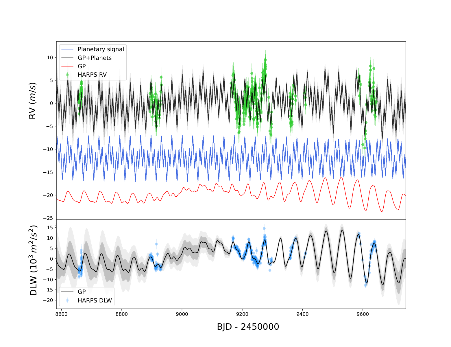
V.3 Multi-dimensional Gaussian process approach
We also followed a multidimensional Gaussian process (GP) approach to account for the stellar signals in our RV time series (Rajpaul et al. 2015). This approach models the RVs along with time series of activity indicators assuming that the same GP, a function , can describe them both. The function represents the projected area of the visible stellar disk that is covered by active regions at a given time. For our best GP analysis, we selected the activity indicator that shows the strongest signal in the periodograms, i.e., the DLW, and modeled the RVs alongside this activity index. We created a two-dimensional GP model via
| (1) | |||
| (2) |
The amplitudes , , and are free parameters, which relate the individual time series to . The RV data are modeled as a function of and its time derivative , since they depend both on the fraction of the stellar surface covered by active regions, and on how these regions evolve and migrate on the disk. The DLW, which measures the width of the spectral lines, has been proven to be a good tracer of the fraction of the surface covered by active regions, and is thus expected to be solely proportional to (Zicher et al. 2022). For our covariance matrix, we used a quasi-periodic kernel
| (3) |
and its derivatives (Barragán et al. 2022; Rajpaul et al. 2015). The parameter PGP in Eq. 3 is the characteristic period of the GP, which is interpreted as the stellar rotation period; is the inverse of the harmonic complexity, which is associated with the distribution of active regions on the stellar surface (Aigrain et al. 2015); is the long-term evolution timescale, i.e., the active region lifetime on the stellar surface. We performed the multidimensional GP regression using pyaneti (Barragán et al. 2022, described in), adding three Keplerians to account for the Doppler reflex motion of the three planets, as described in Sect. V.2.
We performed an MCMC analysis setting informative Gaussian priors based on the transit ephemeris of the innermost planet GJ 367 b, as derived in Sect. V.1, and uniform priors for all the remaining parameters. We also used uniform priors to sample for the multidimensional GP hyper-parameters. We included a jitter term to the diagonal of the covariance for each time series.
We performed our fit with 500 Markov chains to sample the parameter space. The posterior distributions were created using the last 5000 iterations of the converged chains with a thin factor of 10, leading to a distribution of 250,000 data points for each fitted parameter. The chains were initialized at random values within the priors ranges. This ensured a homogeneous sampling of the parameter space.
Priors and results are listed are listed in Table 4. Planets GJ 367 b, c, and d are significantly detected in the HARPS RV time series with Doppler semi-amplitudes of = 0.86 0.15 m s-1, = 1.99 0.17 m s-1, and = 2.03 0.16 m s-1, respectively. These imply planetary masses and minimum masses of = 0.546 0.093 M⊕, = 4.13 0.36 M⊕, and = 6.03 0.49 M⊕. The resulting GP hyper-parameters are PGP = 53.67 days, = 0.44 0.05, and = 114 19 days. The characteristic period PGP is in agreement with the stellar rotation period, as discussed in Sect. III.2, as well as the long-term evolution timescale , which is in agreement with the long-period signal found in the analyses of Sects. IV and V.2.
Figure 8 shows the RV and DLW time series, along with the inferred models, whereas Fig. 9 displays the phase-folded RV curves of the three planets and the best-fitting models.
| Parameter | Prior | Derived value |
|---|---|---|
| GJ 367 b | ||
| Model parameters | ||
| Orbital period [days] | [0.3219225, 0.0000002] | 0.3219225 0.0000002 |
| Transit epoch T0,b [BJD2,450,000] | [8544.1364, 0.0004] | 8544.13631 0.00038 |
| [1.0,1.0] | 0.13 | |
| [1.0,1.0] | 0.05 0.21 | |
| Radial velocity semi-amplitude variation [m s-1] | [0.00, 0.05] | 0.86 0.15 |
| Derived parameters | ||
| Planet mass (∗) | – | 0.546 0.093 |
| Orbit eccentricity | – | 0.10 |
| Argument of periastron of stellar orbit [deg] | – | 71 |
| GJ 367 c | ||
| Model parameters | ||
| Orbital period [days] | [11.4, 11.6] | 11.5301 0.0078 |
| Time of inferior conjunction [BJD2,450,000] | [9153.0, 9155.0] | 9153.84 0.30 |
| [1.0,1.0] | 0.11 | |
| [1.0,1.0] | 0.14 | |
| Radial velocity semi-amplitude variation [m s-1] | [0.00, 0.05] | 1.99 0.17 |
| Derived parameters | ||
| Planet minimum mass | – | 4.13 0.36 |
| Orbit eccentricity | – | 0.09 0.07 |
| Argument of periastron of stellar orbit [deg] | – | 34 |
| GJ 367 d | ||
| Model parameters | ||
| Orbital period [days] | [30.0,40.0] | 34.369 0.073 |
| Time of inferior conjunction [BJD2,450,000] | [9173.0, 9180.0] | 9181.82 1.10 |
| [1.0,1.0] | 0.09 0.19 | |
| [1.0,1.0] | 0.30 | |
| Radial velocity semi-amplitude variation [m s-1] | [0.00, 0.05] | 2.03 0.16 |
| Derived parameters | ||
| Planet minimum mass | – | 6.03 0.49 |
| Orbit eccentricity | – | 0.14 0.09 |
| Argument of periastron of stellar orbit [deg] | – | 126 |
| Additional model parameters | ||
| Characteristic period of the GP [days] | [35.0,65.0] | 53.67 |
| Inverse of the harmonic complexity | [0.1,3.0] | 0.44 0.05 |
| Long-term evolution timescale [days] | [1,300] | 114 19 |
| Amplitude [km s-1] | [0.0,0.005] | 0.0016 0.0004 |
| Amplitude [km s-1] | [0.05,0.05] | 0.009 |
| Amplitude | [0.0,30.0] | 6.31 |
| Systemic velocity [km s-1] | [47.40,48.42] | 47.9168 0.0005 |
| Offset DLW [103 m2 s-2 ] | [16.90,14.11] | 0.11 |
| Radial velocity jitter term [m s-1] | [0,100] | 1.83 0.08 |
| DLW jitter term [m2 s-2] | [0,1000] | 378 |
Note. — refers to uniform priors between and ; refers to Gaussian priors with mean and standard deviation ; refers to Jeffrey’s priors between and . Inferred parameters and uncertainties are defined as the median and the 68.3% credible interval of their posterior distributions.
(∗) Assuming an orbital inclination of = 79.89°, from the modeling of TESS transit light curves (Sect. V.1).
VI Discussion
The three techniques used to determine the mass of GJ 367 b give results that are consistent to within 1. We adopted the results from the FCO method, which gives a planetary mass of = 0.633 0.050 M⊕ (7.9% precision). Our result differs by about 1 from the mass of = 0.546 0.078 M⊕ reported by Lam et al. 2021, which was also derived using the FCO method applied on 20 HARPS data chunks that do not entirely cover the orbital phase of the USP planet, as opposed to our 96 chunks. We found that GJ 367 b has a radius of = 0.699 0.024 R⊕ (3.4% precision), consistent with the value of = 0.718 0.054 R⊕ from Lam et al. 2021, but more precise, thanks to the additional TESS photometry and increased cadence. Lam et al. 2021 reported a density of = 8.1 2.2 g cm-3. The higher mass but similar radius measured in this work make the USP planet denser, with a ultra-high density of = 10.2 1.3 g cm-3.
GJ 367 b belongs to the handful of small USP planets ( 2 R⊕, 10 M⊕) whose masses and radii are known with a precision better than 20%. Figure 10 shows the mass-radius diagram for small USP planets along with the theoretical composition models for rocky worlds (Zeng et al. 2016). GJ 367 b is the smallest and densest USP planet known to date. The position of the planet on the mass-radius diagram suggests that its composition is dominated by iron. Taking into account its mean density, GJ 367 b leads the class of super-Mercuries, namely, extremely dense planets containing an excess of iron, analogous to Mercury: K2-229 b (Santerne et al. 2018), K2-38 b (Toledo-Padrón et al. 2020), K2-106 b (Guenther et al. 2017), Kepler-107 c (Bonomo et al. 2019), Kepler-406 b (Marcy et al. 2014), HD 137496 b (Azevedo Silva et al. 2022), HD 23472 b (Barros et al. 2022), and TOI-1075 b (Essack et al. 2022).
The two non-transiting planets GJ 367 c and GJ 367 d have orbital periods of 11.5 d and 34.4 days, respectively, and minimum masses of = 4.13 0.36 M⊕ and = 6.03 0.49 M⊕, as derived adopting the multidimensional GP approach to model stellar activity (Sect. V.3). We note that our minimum mass determinations are in very good agreement with those of = 4.08 0.30 M⊕ and = 5.93 0.45 M⊕ we determined modeling stellar activity with two sinusoidal components (Sect. V.2).
If the orbits of GJ 367 b, c, and d were coplanar ( = = = 79.9°), planets c and d would have true masses of = 4.19 0.35 M⊕ and = 6.12 0.48 M⊕, respectively. Using the mass-radius relation for small rocky planets from Otegi et al. 2020, we found that GJ 367 c and d are expected to have radii of 1.6 and 1.7 R⊕, respectively, making them two super-Earths with mean densities of 6 g cm-3. We searched the TESS light curves for possible transits of the two outer companions with the DST code (Sect. II.1) masking out the transits of the UPS planet, but we found no other significant transit signals. Under the assumption that the orbits of the three planets are coplanar, the impact parameters of planets c and d would be 6 and 13, respectively. This would account for the non-detection of the transit signals of GJ 367 c and GJ 367 d in the TESS light curves. In this scenario, GJ 367 c and d would transit their host star only if their radii were unphysically large, i.e. and .
The other configuration for the outer planets to transit is if they are mutually inclined with planet b (). This is not an unusual architecture for systems with USP planets (Dai et al. 2018). With minimum masses of 4.13 and 6.03 , GJ 367 c and d are expected to have a minimum radius of 1.5 given the maximum collisional stripping limit (Marcus et al. 2009; Marcus et al. 2010). The inclination of their orbits should be larger than 86.5° to produce non-grazing transits. If the two planets had radii of 1.5 , the transit depths would be 900 ppm. For 2.5 R⊕, the non grazing transit depth is expected to be 2500 ppm. Similarly, transit depth of a 4 planet is ppm. The rms of the TESS light curve of GJ 367 is approximately 500 ppm. The expected transit times of planets c and d also fall well within the baseline of the TESS data. Therefore, GJ 367 c and d would be easily detected if they produced non-grazing transits.
The presence of two additional planetary companions to GJ 367 b is in line with the tendency of USP planets to belong to multi-planet systems (Dai et al. 2021). While the origin of USP planets is debated, it is likely that the presence of outer companions could be responsible for the migration processes that carried USP planets to their current positions (Pu & Lai 2019; Petrovich et al. 2019), which would lie inside the magnetospheric cavity of a typical protoplanetary disk. In these models, planet migration occurs after the dissipation of the protoplanetary disk, by a combination of eccentricity forcing from the planetary companions and tidal dissipation in the innermost planet’s interior, although the precise dynamical forcing mechanisms are debated. Serrano et al. 2022 showed, for TOI-500, that the low-eccentricity secular forcing proposed by Pu & Lai 2019 can explain the migration of that system’s USP planet from a formation radius of 0.02 au to its observed location. For GJ 367 b, we tested this migration scenario with similar initial conditions (USP planet starting at au, initial eccentricities of all planets set to ), and found only modest migration of planet b, from au to 0.01 au, short of the observed au. This would support an alternative migration history, such as by high-eccentricity secular chaos (Petrovich et al. 2019). However, we note that GJ 367 c and GJ 367 d lie close to a 3:1 mean motion commensurability, having a period ratio of 2.98, and that the dynamics may be affected by the 3:1 resonance, which can provide additional eccentricity forcing in the system. A deeper analysis would be needed to draw definite conclusions on the formation, migration, and dynamics of the system. The GJ 367 system is thus an excellent target for studying planetary system formation and evolution scenarios.
VI.1 Internal structure of GJ 367 b

Given the high precision of both the derived mass and radius, we used a Bayesian analysis to infer the internal structure of GJ 367 b. We followed the method described in Leleu et al. 2021, which is based on Dorn et al. 2017. Prior to presenting the results of our modeling, we provide the reader with a brief overview over the used model.
Modeling the interior of an exoplanet is a degenerate problem: there is a multitude of different compositions that could explain the observed planetary density. This is why a Bayesian modeling approach is used, with the goal of finding posterior distributions for the internal structure parameters. We assumed a planet that is made up of four fully distinct layers: an inner iron core, a silicate mantle, a water layer, and a gas layer made up of hydrogen and helium. In our forward model, this atmospheric layer is modeled separately from the rest of the planet following Lopez & Fortney 2014 and it is assumed that it does not influence the inner layers. While the presence of a gas and water layer is not expected given the high equilibrium temperature of GJ 367 b, we still included them in the initial model setup, as this is the most general way to model the planet and give us all possible compositions that could lead to the observed planetary density. As input parameters, we used the planetary and stellar parameters listed in Tables 1 and 2, i.e. the transit depth, RV semi-amplitude and period of the planet and the mass, radius, effective temperature, and metallicity of the star. In addition, we chose a prior distribution of Gyr for the age of the star.
For our Bayesian analysis, we chose a prior that is uniform in log for the gas mass fraction of the planet. For the mass fractions of the inner iron core, the silicate mantle, and the water layer (all with respect to the solid part of the planet without the H/He gas layer), our chosen prior is a distribution that is uniform on the simplex on which these three mass fractions add up to one. Additionally, we added an upper limit of 0.5 for the water mass fraction in the planet, as a planet with a pure water composition is not physical (Thiabaud et al. 2014; Marboeuf et al. 2014). Note that choosing very different priors influences the results of the internal structure analysis.
There are multiple studies that show a correlation between the composition of planets and their host star (Thiabaud et al. 2015; Adibekyan et al. 2021, e.g.), but it is not clear if this correlation is 1:1 or has a different slope. As a first step, we assumed the composition of the planet to match that of its host star exactly. Since we do not have measured values for the stellar [Si/H] and [Mg/H], we left them unconstrained and sampled the stellar parameters from [Si/H] = [Mg/H] . However, our analysis showed that the observed mass and radius values of GJ 367 b are not compatible with a 1:1 relationship between the Si/Mg/Fe ratios of the planet and of these sampled synthetic host stars, as it is not possible to reach such a high density under these constraints. The same is true when assuming the steeper slope between stellar and planetary Fe/(Si+Mg) ratios found by Adibekyan et al. 2021. We then repeated our analysis allowing the iron to silicon and iron to magnesium ratios in the planet to be up to a factor 1000 higher than in the sampled stars.
The results of this second analysis are summarized in Figure 11. Indeed, we can see that the Fe/Si ratio in the planet (and therefore also the Fe/Mg ratio) was a factor of 10 to the power of higher than in the sampled host star. We further expect GJ 367 b to host no H/He envelope and no significant water layer. Conversely, we expect the mass fraction of the inner iron core with (median with 5th and 95th percentiles) to be very high.
VI.2 Formation and evolution of the ultra-high density sub-Earth GJ 367 b
It is not clear how a low-mass high-density planet like GJ 367 b forms. Possible pathways may include the formation out of material significantly more iron rich than thought to be normally present in protoplanetry disks. Although it is not clear if disks with such a large relative iron content specifically near the inner edge (where most of the material might be obtained from) exist (Dullemond & Monnier 2010; Aguichine et al. 2020; Adibekyan et al. 2021)
Another possibility is the formation of a larger planet with a lower bulk density. Subsequently the planet differentiates into a denser core and less dense outer layers. These outer layers are then removed. This may be accomplished through two processes.
(i) A first process is collisional stripping. The preferred removal of outer material in giant collisions (Marcus et al. 2009; Reinhardt et al. 2022, e.g.,) might have increased the bulk density. Indeed, this is what might have lead to the high iron fraction and therefore high density of Mercury for its small size (Benz et al. 1988; Benz et al. 2007), as a Mercury with a chondritic composition would have a lower density. The amount of maximum stripping is governed by the mass, impact velocity, and impact parameter of the impactor (Marcus et al. 2010; Leinhardt & Stewart 2012). Preferable removal of outer layers requires the right mass ratio (close to unity), right impact parameter (close to grazing), and right relative velocity. There is also evidence that, at least in some systems, densities have been altered by collisions (Kepler-107; Bonomo et al. 2019) A problem to effectively remove mass might be the removal of collision debris and the avoidance of a re-accretion of debris material onto the planet, as re-accretion would leave the bulk density largely unchanged. However this might not be such a large problem as originally thought (Spalding & Adams 2020). Our measurement of the bulk density of GJ 367 b suggests that collisional stripping has to be remarkably effective in removing non-iron material from the planet if it is the only process at work.
(ii) A second process that might have played a role in shaping GJ 367 b after core formation is removal of outer layers of material facilitated by the enormous stellar radiation to which this planet is subjected. At the equilibrium temperature of 1365 32 K, material might sublimate, be uplifted, and transported away from the surface.
Of course, all of the above discussed processes could have contributed to create the nearly pure ball of iron, known as GJ 367 b.
VII Conclusions
We report refined mass and radius determinations for GJ 367 b, the ultra-high density, USP sub-Earth planet transiting the M-dwarf star GJ 367 recently discovered by Lam et al. 2021. We used new TESS observations from sectors 35 and 36 combined with 371 Doppler measurements collected as part of an intensive RV follow-up campaign with the HARPS spectrograph. We derived a precise planetary mass of = 0.633 0.050 M⊕ (7.9 % precision) and a radius of = 0.699 0.024 R⊕ (3.4% precision), resulting in an ultra-high density of = 10.2 1.3 g cm-3(13%). According to our internal structure analysis, GJ 367 b is predominantly composed of iron with an iron core mass fraction of 0.91, which accounts for the aforementioned planetary density. In addition, our HARPS RV follow-up observations, which span a period of nearly 3 yr, allowed us to discover two additional non-transiting small companions with orbital periods of 11.5 and 34.4 days, and minimum masses of = 4.13 0.36 M⊕ and = 6.03 0.49 M⊕. GJ 367 joins the small group of well-characterized multiplanetary systems hosting a USP planet, with the inner planet GJ 367 b being the densest and smallest USP planet known to date. This unique multiplanetary system hosting this ultra-high density, USP sub-Earth is an extraordinary target to further investigate the formation and migration scenarios of USP systems.
Acknowledgments: We thank the anonymous referee for a thoughtful review of our paper and very positive feedback. This work was supported by the KESPRINT collaboration, an international consortium devoted to the characterization and research of exoplanets discovered with space-based missions (www.kesprint.science). Based on observations made with the ESO-3.6 m telescope at La Silla Observatory under programs 1102.C-0923 and 106.21TJ.001. We are extremely grateful to the ESO staff members for their unique and superb support during the observations. We acknowledge the use of public TESS data from pipelines at the TESS Science Office and at the TESS Science Processing Operations Center. TESS data presented in this paper were obtained from the Milkulski Archive for Space Telescopes (MAST) at the Space Telescope Science Institute. The specific observations analyzed can be accessed via https://doi.org/10.17909/rkwv-t847 (catalog DOI: 10.17909/rkwv-t847). Resources supporting this work were provided by the NASA High-End Computing (HEC) Program through the NASA Advanced Supercomputing (NAS) Division at Ames Research Center for the production of the SPOC data products. E.G. acknowledges the generous support from Deutsche Forschungsgemeinschaft (DFG) of the grant HA3279/14-1. D.G. gratefully acknowledges financial support from the Cassa di Risparmio di Torino (CRT) foundation under Grant No. 2018.2323 “Gaseous or rocky? Unveiling the nature of small worlds”. Y.A. and J.A.E. acknowledge the support of the Swiss National Fund under grant 200020_192038. C.M.P. gratefully acknowledges the support of the Swedish National Space Agency (DNR 65/19). R.L. acknowledges funding from University of La Laguna through the Margarita Salas Fellowship from the Spanish Ministry of Universities ref. UNI/551/2021-May 26, and under the EU Next Generation funds. K.W.F.L. was supported by Deutsche Forschungsgemeinschaft grants RA714/14-1 within the DFG Schwerpunkt SPP 1992, Exploring the Diversity of Extrasolar Planets. S.A. acknowledges the support from the Danish Council for Independent Research through a grant No.2032-00230B. O.B. acknowledges that has received funding from the ERC under the European Union’s Horizon 2020 research and innovation program (grant agreement No. 865624). H.J.D. acknowledges support from the Spanish Research Agency of the Ministry of Science and Innovation (AEI-MICINN) under grant ’Contribution of the IAC to the PLATO Space Mission’ with reference PID2019-107061GB-C66. A.J.M. acknowledges support from the Swedish National Space Agency (career grant 120/19C). O.K. acknowledges support by the Swedish Research Council (grant agreement No. 2019-03548), the Swedish National Space Agency, and the Royal Swedish Academy of Sciences J.K. gratefully acknowledges the support of the Swedish National Space Agency (SNSA; DNR 2020-00104) and of the Swedish Research Council (VR: Etableringsbidrag 2017-04945).
We report here the HARPS RVs, including those previously reported in Lam et al. 2021, along with the activity indicators and line profile variation diagnostics extracted with NAIRA and serval (5). Time stamps are given in Barycentric Julian Date in the Barycentric Dynamical Time (BJDTDB).
| BJDTBD | RV | H | H | H | log R | NaD | DLW | CRX | ||||||||
|---|---|---|---|---|---|---|---|---|---|---|---|---|---|---|---|---|
| -2450000 | () | () | (Ang) | (Ang) | (Ang) | (Ang) | (Ang) | (Ang) | (Ang) | (Ang) | () | () | () | () | ||
| 8658.45473 | 47.91637 | 0.00084 | 0.06472 | 0.00012 | 0.05217 | 0.00026 | 0.11412 | 0.00081 | -5.222 | 0.077 | 0.01038 | 0.00007 | -7.9 | 1.3 | -10.2 | 11.1 |
| 8658.46195 | 47.91814 | 0.00082 | 0.06421 | 0.00011 | 0.05180 | 0.00025 | 0.11147 | 0.00078 | -5.180 | 0.077 | 0.01040 | 0.00007 | -10.0 | 1.2 | 3.4 | 9.3 |
| 8658.46946 | 47.91502 | 0.00085 | 0.06424 | 0.00012 | 0.05180 | 0.00026 | 0.11413 | 0.00084 | -5.221 | 0.077 | 0.01045 | 0.00007 | -6.8 | 1.2 | -17.2 | 10.7 |
| 8658.47642 | 47.91611 | 0.00079 | 0.06417 | 0.00011 | 0.05257 | 0.00025 | 0.11363 | 0.00078 | -5.130 | 0.077 | 0.01041 | 0.00007 | -7.1 | 1.3 | 2.8 | 10.9 |
| 8658.48401 | 47.91860 | 0.00090 | 0.06454 | 0.00012 | 0.05315 | 0.00028 | 0.11124 | 0.00088 | -5.139 | 0.077 | 0.01040 | 0.00008 | -7.5 | 1.4 | 3.5 | 11.0 |
| 8658.49105 | 47.91862 | 0.00087 | 0.06499 | 0.00012 | 0.05417 | 0.00027 | 0.11592 | 0.00086 | -5.136 | 0.077 | 0.01054 | 0.00007 | -6.1 | 1.3 | 4.4 | 10.9 |
| 8658.49842 | 47.91780 | 0.00086 | 0.06548 | 0.00012 | 0.05403 | 0.00027 | 0.11601 | 0.00088 | -5.151 | 0.077 | 0.01074 | 0.00007 | -7.9 | 1.1 | -11.5 | 10.4 |
| 8658.50565 | 47.91753 | 0.00091 | 0.06500 | 0.00012 | 0.05374 | 0.00029 | 0.11864 | 0.00092 | -5.137 | 0.077 | 0.01066 | 0.00008 | -5.0 | 1.5 | 9.4 | 11.2 |
| 8658.51297 | 47.91784 | 0.00089 | 0.06466 | 0.00012 | 0.05302 | 0.00028 | 0.11529 | 0.00091 | -5.175 | 0.077 | 0.01057 | 0.00008 | -9.3 | 1.3 | -15.4 | 10.6 |
| 8658.52049 | 47.91557 | 0.00083 | 0.06464 | 0.00011 | 0.05272 | 0.00026 | 0.11484 | 0.00085 | -5.151 | 0.077 | 0.01069 | 0.00007 | -5.7 | 1.3 | 6.2 | 11.1 |
| … | … | … | … | … | … | … | … | … | … | … | … | … | … | … | … | … |
Note. — The entire RV data set is available in its entirety in machine-readable form. Only a portion of this table is shown here to demonstrate its form and content.
References
- Adams et al. (2017) Adams, E. R., Jackson, B., Endl, M., et al. 2017, The Astronomical Journal, 153, 82, doi: 10.3847/1538-3881/153/2/82
- Adibekyan et al. (2021) Adibekyan, V., Dorn, C., Sousa, S. G., et al. 2021, Science, 374, 330, doi: 10.1126/science.abg8794
- Aguichine et al. (2020) Aguichine, A., Mousis, O., Devouard, B., & Ronnet, T. 2020, ApJ, 901, 97, doi: 10.3847/1538-4357/abaf47
- Aguirre Børsen-Koch et al. (2022) Aguirre Børsen-Koch, V., Rørsted, J. L., Justesen, A. B., et al. 2022, MNRAS, 509, 4344, doi: 10.1093/mnras/stab2911
- Aigrain et al. (2015) Aigrain, S., Llama, J., Ceillier, T., et al. 2015, MNRAS, 450, 3211, doi: 10.1093/mnras/stv853
- Anderson et al. (2010) Anderson, D. R., Cameron, A. C., Hellier, C., et al. 2010, ApJL, 726, L19, doi: 10.1088/2041-8205/726/2/l19
- Astudillo-Defru et al. (2017a) Astudillo-Defru, N., Delfosse, X., Bonfils, X., et al. 2017a, A&A, 600, A13, doi: 10.1051/0004-6361/201527078
- Astudillo-Defru et al. (2017b) Astudillo-Defru, N., Forveille, T., Bonfils, X., et al. 2017b, A&A, 602, A88, doi: 10.1051/0004-6361/201630153
- Azevedo Silva et al. (2022) Azevedo Silva, T., Demangeon, O. D. S., Barros, S. C. C., et al. 2022, A&A, 657, A68, doi: 10.1051/0004-6361/202141520
- Bagnulo et al. (2009) Bagnulo, S., Landolfi, M., Landstreet, J. D., et al. 2009, PASP, 121, 993, doi: 10.1086/605654
- Barnes (2010) Barnes, S. A. 2010, ApJ, 722, 222, doi: 10.1088/0004-637X/722/1/222
- Barnes & Kim (2010) Barnes, S. A., & Kim, Y.-C. 2010, ApJ, 721, 675, doi: 10.1088/0004-637X/721/1/675
- Barragán et al. (2022) Barragán, O., Aigrain, S., Rajpaul, V. M., & Zicher, N. 2022, MNRAS, 509, 866, doi: 10.1093/mnras/stab2889
- Barragán et al. (2019) Barragán, O., Gandolfi, D., & Antoniciello, G. 2019, MNRAS, 482, 1017, doi: 10.1093/mnras/sty2472
- Barragán et al. (2018) Barragán, O., Gandolfi, D., Dai, F., et al. 2018, A&A, 612, A95, doi: 10.1051/0004-6361/201732217
- Barros et al. (2022) Barros, S. C. C., Demangeon, O. D. S., Alibert, Y., et al. 2022, A&A, 665, A154, doi: 10.1051/0004-6361/202244293
- Benz et al. (2007) Benz, W., Anic, A., Horner, J., & Whitby, J. A. 2007, Space Science Reviews, 132, 189, doi: 10.1007/s11214-007-9284-1
- Benz et al. (1988) Benz, W., Slattery, W. L., & Cameron, A. G. W. 1988, Icarus, 74, 516, doi: 10.1016/0019-1035(88)90118-2
- Binks & Jeffries (2014) Binks, A. S., & Jeffries, R. D. 2014, MNRAS, 438, L11, doi: 10.1093/mnrasl/slt141
- Binks et al. (2021) Binks, A. S., Jeffries, R. D., Jackson, R. J., et al. 2021, MNRAS, 505, 1280, doi: 10.1093/mnras/stab1351
- Bonomo et al. (2019) Bonomo, A. S., Zeng, L., Damasso, M., et al. 2019, NatAs, 3, 416, doi: 10.1038/s41550-018-0684-9
- Brandner et al. (2022) Brandner, W., Calissendorff, P., Frankel, N., & Cantalloube, F. 2022, MNRAS, 513, 661, doi: 10.1093/mnras/stac961
- Cabrera et al. (2012) Cabrera, J., Csizmadia, S., Erikson, A., Rauer, H., & Kirste, S. 2012, A&A, 548, A44, doi: 10.1051/0004-6361/201219337
- Cifuentes et al. (2020) Cifuentes, C., Caballero, J. A., Cortés-Contreras, M., et al. 2020, A&A, 642, A115, doi: 10.1051/0004-6361/202038295
- Claret (2017) Claret, A. 2017, A&A, 600, A30, doi: 10.1051/0004-6361/201629705
- Dai et al. (2018) Dai, F., Masuda, K., & Winn, J. N. 2018, ApJL, 864, L38, doi: 10.3847/2041-8213/aadd4f
- Dai et al. (2021) Dai, F., Howard, A. W., Batalha, N. M., et al. 2021, AJ, 162, 62, doi: 10.3847/1538-3881/ac02bd
- Donati et al. (1997) Donati, J. F., Semel, M., Carter, B. D., Rees, D. E., & Collier Cameron, A. 1997, MNRAS, 291, 658, doi: 10.1093/mnras/291.4.658
- Donati et al. (2008) Donati, J. F., Morin, J., Petit, P., et al. 2008, MNRAS, 390, 545, doi: 10.1111/j.1365-2966.2008.13799.x
- Dorn et al. (2017) Dorn, C., Venturini, J., Khan, A., et al. 2017, A&A, 597, A37, doi: 10.1051/0004-6361/201628708
- Dullemond & Monnier (2010) Dullemond, C. P., & Monnier, J. D. 2010, Annual Review of Astronomy and Astrophysics, 48, 205, doi: 10.1146/annurev-astro-081309-130932
- Essack et al. (2022) Essack, Z., Burt, J., Shporer, A., et al. 2022, in Bulletin of the American Astronomical Society, Vol. 54, 102.59
- Gaia Collaboration et al. (2021) Gaia Collaboration, Smart, R. L., Sarro, L. M., et al. 2021, A&A, 649, A6, doi: 10.1051/0004-6361/202039498
- Gaidos et al. (2023) Gaidos, E., Claytor, Z., Dungee, R., Ali, A., & Feiden, G. A. 2023, MNRAS, doi: 10.1093/mnras/stad343
- Gandolfi et al. (2017) Gandolfi, D., Barragá n, O., Hatzes, A. P., et al. 2017, The Astronomical Journal, 154, 123, doi: 10.3847/1538-3881/aa832a
- Guenther et al. (2017) Guenther, E. W., Barragán, O., Dai, F., et al. 2017, A&A, 608, A93, doi: 10.1051/0004-6361/201730885
- Hatzes (2019) Hatzes, A. P. 2019, The Doppler Method for the Detection of Exoplanets, doi: 10.1088/2514-3433/ab46a3
- Hatzes et al. (2010) Hatzes, A. P., Dvorak, R., Wuchterl, G., et al. 2010, Astronomy and Astrophysics, 520, A93, doi: 10.1051/0004-6361/201014795
- Hatzes et al. (2011) Hatzes, A. P., Fridlund, M., Nachmani, G., et al. 2011, ApJ, 743, 75, doi: 10.1088/0004-637X/743/1/75
- Hidalgo et al. (2018) Hidalgo, S. L., Pietrinferni, A., Cassisi, S., et al. 2018, ApJ, 856, 125, doi: 10.3847/1538-4357/aab158
- Hirano et al. (2018) Hirano, T., Dai, F., Gandolfi, D., et al. 2018, AJ, 155, 127, doi: 10.3847/1538-3881/aaa9c1
- Hirano et al. (2021) Hirano, T., Livingston, J. H., Fukui, A., et al. 2021, AJ, 162, 161, doi: 10.3847/1538-3881/ac0fdc
- Jenkins et al. (2016) Jenkins, J. M., Twicken, J. D., McCauliff, S., et al. 2016, in Proc. SPIE, Vol. 9913, Software and Cyberinfrastructure for Astronomy IV, 99133E, doi: 10.1117/12.2233418
- Kiman et al. (2021) Kiman, R., Faherty, J. K., Cruz, K. L., et al. 2021, AJ, 161, 277, doi: 10.3847/1538-3881/abf561
- Klein et al. (2022) Klein, B., Zicher, N., Kavanagh, R. D., et al. 2022, MNRAS, 512, 5067, doi: 10.1093/mnras/stac761
- Kochukhov (2021) Kochukhov, O. 2021, A&A Rev., 29, 1, doi: 10.1007/s00159-020-00130-3
- Kochukhov et al. (2010) Kochukhov, O., Makaganiuk, V., & Piskunov, N. 2010, A&A, 524, A5, doi: 10.1051/0004-6361/201015429
- Kochukhov & Reiners (2020) Kochukhov, O., & Reiners, A. 2020, ApJ, 902, 43, doi: 10.3847/1538-4357/abb2a2
- Koen et al. (2010) Koen, C., Kilkenny, D., van Wyk, F., & Marang, F. 2010, MNRAS, 403, 1949, doi: 10.1111/j.1365-2966.2009.16182.x
- Lam et al. (2021) Lam, K. W. F., Csizmadia, S., Astudillo-Defru, N., et al. 2021, Science, 374, 1271–1275, doi: 10.1126/science.aay3253
- Lee & Chiang (2017) Lee, E. J., & Chiang, E. 2017, The Astrophysical Journal, 842, 40, doi: 10.3847/1538-4357/aa6fb3
- Leinhardt & Stewart (2012) Leinhardt, Z. M., & Stewart, S. T. 2012, The Astrophysical Journal, 745, 79, doi: 10.1088/0004-637X/745/1/79
- Leleu et al. (2021) Leleu, A., Alibert, Y., Hara, N. C., et al. 2021, A&A, 649, A26, doi: 10.1051/0004-6361/202039767
- Lopez & Fortney (2014) Lopez, E. D., & Fortney, J. J. 2014, ApJ, 792, 1, doi: 10.1088/0004-637X/792/1/1
- Lovis & Pepe (2007) Lovis, C., & Pepe, F. 2007, A&A, 468, 1115, doi: 10.1051/0004-6361:20077249
- Mamajek & Bell (2014) Mamajek, E. E., & Bell, C. P. M. 2014, MNRAS, 445, 2169, doi: 10.1093/mnras/stu1894
- Mandel & Agol (2002) Mandel, K., & Agol, E. 2002, ApJL, 580, L171–L175, doi: 10.1086/345520
- Mann et al. (2015) Mann, A. W., Feiden, G. A., Gaidos, E., Boyajian, T., & von Braun, K. 2015, ApJ, 804, 64, doi: 10.1088/0004-637X/804/1/64
- Mann et al. (2019) Mann, A. W., Dupuy, T., Kraus, A. L., et al. 2019, ApJ, 871, 63, doi: 10.3847/1538-4357/aaf3bc
- Marboeuf et al. (2014) Marboeuf, U., Thiabaud, A., Alibert, Y., Cabral, N., & Benz, W. 2014, A&A, 570, A36, doi: 10.1051/0004-6361/201423431
- Marcus et al. (2010) Marcus, R. A., Sasselov, D., Hernquist, L., & Stewart, S. T. 2010, ApJL, 712, L73, doi: 10.1088/2041-8205/712/1/L73
- Marcus et al. (2009) Marcus, R. A., Stewart, S. T., Sasselov, D., & Hernquist, L. 2009, ApJL, 700, L118, doi: 10.1088/0004-637X/700/2/L118
- Marcy et al. (2014) Marcy, G. W., Isaacson, H., Howard, A. W., et al. 2014, ApJS, 210, 20, doi: 10.1088/0067-0049/210/2/20
- Mayor et al. (2003) Mayor, M., Pepe, F., Queloz, D., et al. 2003, The Messenger, 114, 20
- Millholland & Spalding (2020) Millholland, S. C., & Spalding, C. 2020, The Astrophysical Journal, 905, 71, doi: 10.3847/1538-4357/abc4e5
- Morin et al. (2008) Morin, J., Donati, J. F., Petit, P., et al. 2008, MNRAS, 390, 567, doi: 10.1111/j.1365-2966.2008.13809.x
- Murdoch et al. (1993) Murdoch, K. A., Hearnshaw, J. B., & Clark, M. 1993, The Astrophysical Journal, 413, 349, doi: 10.1086/173003
- Otegi et al. (2020) Otegi, J. F., Bouchy, F., & Helled, R. 2020, A&A, 634, A43, doi: 10.1051/0004-6361/201936482
- Pace (2013) Pace, G. 2013, A&A, 551, L8, doi: 10.1051/0004-6361/201220364
- Paegert et al. (2022) Paegert, M., Stassun, K. G., Collins, K. A., et al. 2022, VizieR Online Data Catalog, IV/39
- Petrovich et al. (2019) Petrovich, C., Deibert, E., & Wu, Y. 2019, The Astronomical Journal, 157, 180, doi: 10.3847/1538-3881/ab0e0a
- Piskunov et al. (2011) Piskunov, N., Snik, F., Dolgopolov, A., et al. 2011, The Messenger, 143, 7
- Piskunov & Valenti (2002) Piskunov, N. E., & Valenti, J. A. 2002, A&A, 385, 1095, doi: 10.1051/0004-6361:20020175
- Pu & Lai (2019) Pu, B., & Lai, D. 2019, Monthly Notices of the Royal Astronomical Society, 488, 3568–3587, doi: 10.1093/mnras/stz1817
- Rajpaul et al. (2015) Rajpaul, V., Aigrain, S., Osborne, M. A., Reece, S., & Roberts, S. 2015, Monthly Notices of the Royal Astronomical Society, 452, 2269, doi: 10.1093/mnras/stv1428
- Reinhardt et al. (2022) Reinhardt, C., Meier, T., Stadel, J. G., Otegi, J. F., & Helled, R. 2022, Monthly Notices of the Royal Astronomical Society, 517, 3132, doi: 10.1093/mnras/stac1853
- Ricker et al. (2015) Ricker, G. R., Winn, J. N., Vanderspek, R., et al. 2015, Journal of Astronomical Telescopes, Instruments, and Systems, 1, 014003, doi: 10.1117/1.JATIS.1.1.014003
- Rodriguez et al. (2018) Rodriguez, J. E., Becker, J. C., Eastman, J. D., et al. 2018, The Astronomical Journal, 156, 245, doi: 10.3847/1538-3881/aae530
- Rusomarov et al. (2013) Rusomarov, N., Kochukhov, O., Piskunov, N., et al. 2013, A&A, 558, A8, doi: 10.1051/0004-6361/201220950
- Ryabchikova et al. (2015) Ryabchikova, T., Piskunov, N., Kurucz, R. L., et al. 2015, Phys. Scr, 90, 054005, doi: 10.1088/0031-8949/90/5/054005
- Sahu et al. (2006) Sahu, K. C., Casertano, S., Bond, H. E., et al. 2006, Nature, 443, 534, doi: 10.1038/nature05158
- Sanchis-Ojeda et al. (2014) Sanchis-Ojeda, R., Rappaport, S., Winn, J. N., et al. 2014, The Astrophysical Journal, 787, 47, doi: 10.1088/0004-637x/787/1/47
- Santerne et al. (2018) Santerne, A., Brugger, B., Armstrong, D. J., et al. 2018, NatAs, 2, 393, doi: 10.1038/s41550-018-0420-5
- Schlaufman et al. (2010) Schlaufman, K. C., Lin, D. N. C., & Ida, S. 2010, ApJL, 724, L53–L58, doi: 10.1088/2041-8205/724/1/l53
- Serrano et al. (2022) Serrano, L. M., Gandolfi, D., Mustill, A. J., et al. 2022, NatAs, 6, 736, doi: 10.1038/s41550-022-01641-y
- Smith et al. (2012) Smith, J. C., Stumpe, M. C., Van Cleve, J. E., et al. 2012, PASP, 124, 1000, doi: 10.1086/667697
- Snik et al. (2011) Snik, F., Kochukhov, O., Piskunov, N., et al. 2011, in Astronomical Society of the Pacific Conference Series, Vol. 437, Astronomical Society of the Pacific Conference Series, ed. J. R. Kuhn et al., 237. https://arxiv.org/abs/1010.0397
- Southworth (2011) Southworth, J. 2011, MNRAS, 417, 2166, doi: 10.1111/j.1365-2966.2011.19399.x
- Spalding & Adams (2020) Spalding, C., & Adams, F. C. 2020, The Planetary Science Journal, 1, 7, doi: 10.3847/PSJ/ab781f
- Stassun et al. (2018) Stassun, K. G., Oelkers, R. J., Pepper, J., et al. 2018, AJ, 156, 102, doi: 10.3847/1538-3881/aad050
- Stassun et al. (2019) Stassun, K. G., Oelkers, R. J., Paegert, M., et al. 2019, AJ, 158, 138, doi: 10.3847/1538-3881/ab3467
- Stumpe et al. (2014) Stumpe, M. C., Smith, J. C., Catanzarite, J. H., et al. 2014, Publications of the Astronomical Society of the Pacific, 126, 100. http://www.jstor.org/stable/10.1086/674989
- Stumpe et al. (2012) Stumpe, M. C., Smith, J. C., Van Cleve, J. E., et al. 2012, PASP, 124, 985, doi: 10.1086/667698
- Thiabaud et al. (2014) Thiabaud, A., Marboeuf, U., Alibert, Y., et al. 2014, A&A, 562, A27, doi: 10.1051/0004-6361/201322208
- Thiabaud et al. (2015) Thiabaud, A., Marboeuf, U., Alibert, Y., Leya, I., & Mezger, K. 2015, A&A, 580, A30, doi: 10.1051/0004-6361/201525963
- Toledo-Padrón et al. (2020) Toledo-Padrón, B., Lovis, C., Suárez Mascareño, A., et al. 2020, A&A, 641, A92, doi: 10.1051/0004-6361/202038187
- Triaud (2018) Triaud, A. H. M. J. 2018, in Handbook of Exoplanets, ed. H. J. Deeg & J. A. Belmonte, 2, doi: 10.1007/978-3-319-55333-7_2
- Wildi et al. (2010) Wildi, F., Pepe, F., Chazelas, B., Lo Curto, G., & Lovis, C. 2010, in Society of Photo-Optical Instrumentation Engineers (SPIE) Conference Series, Vol. 7735, Ground-based and Airborne Instrumentation for Astronomy III, ed. I. S. McLean, S. K. Ramsay, & H. Takami, 77354X, doi: 10.1117/12.857951
- Wildi et al. (2011) Wildi, F., Pepe, F., Chazelas, B., Lo Curto, G., & Lovis, C. 2011, in Society of Photo-Optical Instrumentation Engineers (SPIE) Conference Series, Vol. 8151, Techniques and Instrumentation for Detection of Exoplanets V, ed. S. Shaklan, 81511F, doi: 10.1117/12.901550
- Winn (2010) Winn, J. N. 2010, arXiv e-prints, arXiv:1001.2010, doi: 10.48550/arXiv.1001.2010
- Winn & Fabrycky (2015) Winn, J. N., & Fabrycky, D. C. 2015, Annual Review of Astronomy and Astrophysics, 53, 409, doi: 10.1146/annurev-astro-082214-122246
- Winn et al. (2018) Winn, J. N., Sanchis-Ojeda, R., & Rappaport, S. 2018, New Astronomy Reviews, 83, 37, doi: https://doi.org/10.1016/j.newar.2019.03.006
- Yee et al. (2017) Yee, S. W., Petigura, E. A., & von Braun, K. 2017, ApJ, 836, 77, doi: 10.3847/1538-4357/836/1/77
- Zechmeister & Kürster (2009) Zechmeister, M., & Kürster, M. 2009, Astronomy & Astrophysics, 496, 577–584, doi: 10.1051/0004-6361:200811296
- Zechmeister et al. (2017) Zechmeister, M., Reiners, A., Amado, P. J., et al. 2017, Astronomy & Astrophysics, 609, A12, doi: 10.1051/0004-6361/201731483
- Zeng et al. (2016) Zeng, L., Sasselov, D. D., & Jacobsen, S. B. 2016, ApJ, 819, 127, doi: 10.3847/0004-637X/819/2/127
- Zhu & Dong (2021) Zhu, W., & Dong, S. 2021, ARA&A, 59, 291, doi: 10.1146/annurev-astro-112420-020055
- Zicher et al. (2022) Zicher, N., Barragán, O., Klein, B., et al. 2022, MNRAS, 512, 3060, doi: 10.1093/mnras/stac614