Efficient Strongly Polynomial Algorithms for Quantile Regression
Abstract
Linear Regression is a seminal technique in statistics and machine learning, where the objective is to build linear predictive models between a response (i.e., dependent) variable and one or more predictor (i.e., independent) variables. One of the classical and widely used approaches is Ordinary Least Square Regression (OLS). In this paper, we revisit another classical approach, Quantile Regression (QR), which is statistically a more robust alternative to OLS. However, while there exist efficient algorithms for OLS, the state-of-art algorithms for QR require solving large linear programs using interior point methods which are weakly polynomial.
Towards filling this gap, this paper proposes several efficient strongly polynomial algorithms for QR for various settings. For two dimensional QR (i.e., one dependent and one independent variable), we make a connection to the geometric concept of -set, and propose an algorithm with a deterministic worst-case time complexity of and an expected time complexity of for the randomized version. We also propose a randomized divide-and-conquer algorithm - RandomizedQR with an expected time complexity of for the two dimensional QR problem. For the -dimensional QR problem (i.e., one dependent and independent variables), our RandomizedQR algorithm has an expected time complexity of .
1 Introduction
Linear Regression is a seminal technique in statistics and machine learning, where the objective is to build linear predictive models between a response (i.e., dependent) variable and one or more predictor (i.e., independent) variables from a given dataset of instances, where each instance is a set of values of the independent variables and the corresponding value of the dependent variable. One of the classical and widely used approaches is Ordinary Least Square Regression (OLS), where the objective is the minimize the average squared error between the predicted and actual value of the dependent variable. Another classical approach is Quantile Regression (QR), where the objective is to minimize the average weighted absolute error between the predicted and actual value of the dependent variable. QR (also known as “Median Regression” for the special case of the middle quantile), is less affected by outliers and thus statistically a more robust alternative to OLS [18, 15]. However, while there exist efficient algorithms for OLS, the state-of-art algorithms for QR require solving large linear programs with many variables and constraints. They can be solved using using interior point methods [24] which are weakly polynomial (i.e., in the arithmetic computation model the running time is polynomial in the number of bits required to represent the rational numbers in the input), or using Simplex-based exterior point methods which can have exponential time complexity in the worst case [10].
The main focus of our paper is an investigation of the computational complexity of Quantile Regression, and in particular, to design efficient strongly polynomial algorithms (i.e., in the arithmetic computation model the running time is polynomial in the number of rational numbers in the input) for various special cases of the problem.
1.1 Prior Work
In prior work, Barrodale and Robert (BR) proposed a Simplex-based exterior point technique [1], which moves from one exterior point (i.e., a “corner” of the feasible polytope defined by the linear program) to another exterior point, in the direction of steepest gradient descent. The core idea of BR originates from Edgeworth’s bi-variate weighted median based approach [13]. For the special case of the 2-dimensional QR problem (i.e., one dependent variable and one independent variable), the time complexity of this algorithm is , which is still the best known strongly polynomial result for 2-dimensions. For the general -dimensional QR problem (i.e., one dependent variable and independent variables), the best known strongly polynomial algorithm is a naive baseline method that runs in time (note that this assumes the dimension is bounded). Later, Portnoy and Koenkar proposed the interior point method (IPM) which finds the optimal solution by minimizing the difference between primal and dual objective cost [24]. This method is reasonably fast for larger input sizes in practice, but the worst-case theoretical time complexity is where is the desired accuracy, which needs to be set to to obtain the optimal result, where is the number of bits in the input instance [29]. Thus, while the worst case time complexity is independent of the dimension of the QR problem, it is weakly polynomial. Moreover, as shall be clear in later sections, even for a low-dimensional QR problem, e.g., , the corresponding LP formulation can be extremely high-dimensional, since it requires the addition of variables. Thus, one cannot leverage well-known efficient and strongly polynomial low-dimensional LP algorithms for solving low dimensional QR problems.
| Dimension | Weakly polynomial | Strongly Polynomial |
|---|---|---|
| LP - [17] | [1] | |
| General | LP - [27] | Baseline - |
Table 1 provides a snapshot of the computational complexity of these prior techniques. Besides these results, there have been prior research on QR algorithms under various distributional assumptions of the input data, which are less relevant to the focus of our paper. We discuss the challenges and some of the state of the art techniques in Appendix A.
1.2 Our Technical Contributions
In this paper, we make the following key technical contributions that give rise to several strongly polynomial algorithms.
Our first contribution is to capitalize on the computational geometry concepts of arrangement and duality [11], and map QR via a duality transform into a problem of traversing an arrangement of hyperplanes in search of the intersection point that optimizes the QR objective function. To aid this traversal, we leverage the specifics of the QR objective function and design an algorithm named UpdateNeighbor subroutine, which can update the objective function calculations from a neighboring point in the arrangement very efficiently with time and space complexity (i.e., each update is independent of ). This is done by maintaining various aggregate information along every feature. This UpdateNeighbor subroutine allows us to easily improve the naive baseline QR algorithm’s running time from to .
Our second contribution is to connect the QR problem with the concept of geometric -sets [11], which allows our algorithm to restrict its traversal to within the level of the arrangement. In our case, the parameter is set to the quantile, e.g., for median regression, . This connection with -sets gives rise to an efficient quantile regression algorithm for 2-dimension, named QReg2D. The deterministic time complexity for our QR algorithm is where is an arbitrarily small constant. If we use probabilistic -set enumeration procedures in our algorithm, the expected time complexity of our algorithm is . These are asymptotically better than any other existing exterior or interior point approaches in two dimensions (recall that BR runs in time while IPM runs in time). In higher dimensions, counting as well as efficiently enumerating -sets are generally challenging and open problems in computational geometry. Any breakthroughs are likely to have implications in our -set based algorithms for higher dimensional QR problems.
Our third contribution is a probabilistic RandomizedQR algorithm for the QR problem in general dimensions. We devise a divide-and-conquer approach to split the dimensional arrangement into two half-spaces based on a randomly chosen hyperplane and determine the half-space that contains the optimal solution. The highlights of our approach include developing an efficient probabilistic technique for sampling uniformly at random vertices contrained within a portion of the arrangement, which we further connect to the problem of counting inversions of a permutation. Our RandomizedQR algorithm has an expected time complexity of for two dimensions which is asymptotically better than the other strongly and weakly polynomial algorithms. The time complexity of RandomizedQR in higher dimensions is , which is faster than the known deterministic strongly polynomial algorithms.
A summary of the time complexities of our algorithms is presented in Table 2.
2 Preliminaries
In this section, we provide useful definitions and notations, as well as a formal description of the main problem considered in this paper. Some of the notations and formal problem definitions are borrowed from existing literature such as [1, 24].
2.1 Running Example
| 3.15 | 3.13 | |
| 1.97 | 1 | |
| 1.369 | 2.43 | |
| 0.149 | 1.287 | |
| -0.39 | 0.222 | |
| -0.51 | -0.65 | |
| -2.04 | 7.30 |
In this paper, we use a toy dataset, shown in Table 3, which will be used throughout the paper. Assume that we want to build a linear model to predict from . Figure 4 shows a scatter plot of the data points in 2-dimensional space (where the -axis is and -axis is ), and two linear models, one being the classical OLS model and the other being the classical QR model. The former minimizes the sum of squared errors, while the latter minimizes the sum of absolute errors (this is also known as -regression), where the error is defined as the difference between the actual and predicted value of the variable. The figure shows that the OLS model is heavily affected by the presence of outlier , however, the -regression is less sensitive to the outlier.
2.2 Quantile Regression Problem Definition
Dataset: Let be a dataset with points and numerical variables. We denote the response variable and the vector of predictor variables by and respectively for point. A constant is added in to make the problem definition (defined later) consistent. is a matrix where row corresponds to . and for the running example are shown in Figure 1.
Residual: If the actual value is and the predicted value is , then the residual, , can be defined as . The value of can be positive, negative, or zero. From this viewpoint, we can also define where, for each point in , and . The dotted lines in Figure 4 show the residuals. has positive residual and has negative residual.
Quantile Parameter, : In Quantile Regression, the quantile parameter determines what fraction of a total number of input points will have a negative residual. For , half of the input point will have negative residuals, and the remaining half will have positive residuals.
Formal Problem Definition: The formal definition of Quantile Linear Regression (QR) problem in this paper is defined as follows.
In Figure 4, we used for the QR which puts equal penalty for both positive and negative residuals. For , QR is known as -regression (also known as median regression). Different applications may require different values of . For example, if , the objective function puts a high penalty (0.95) on any point with positive residual and a low penalty (0.05) on any point with negative residual.
One of the common techniques that has been used to solve the QR problem is Linear Programming. In the LP formulation, variables are introduced, one for each of the residuals. Additionally, variables are needed for the optimal QR hyperplane parameters . The LP formulation for the QR problem is given in Figure 2:
min sub ject to
Based on the LP formulation, even if we assume is bounded, there are variables and constraints. As the number of variables translate to dimensions in LP and is not a fixed number, the QR problem cannot use some of the strongly polynomial LP results for fixed dimensions. Table 1 summarizes some of latest results for the weakly polynomial LP techniques when applied to QR problem. A detailed description of the current state of the art algorithms for QR is presented in Appendix B.1.


2.3 Other Useful Notations
In this section, we define the dual space of , its connection with the quantile regression problem, and some of the basic properties and definitions that we will use throughout the paper.
QR Hyperplane, : LR estimates the response variable as a linear combination of predictor variables with an offset. The hyperplane that minimizes the optimization function is called a QR Hyperplane and denoted by As shown in Figure 4,for our running example in 2-dimensions, the regression hyperplanes are lines. The coefficients associated with the QR Hyperplane are regression parameters ().
Optimal QR Hyperplane, : In primal space, there is a QR hyperplane for which QR optimization function is minimum. We call this hyperplane Optimal QR Hyperplane and denote it by . The Optimal QR Hyperplane geometrically divides the points into points on one side and points on the other side [20].
The following two important QR properties are used throughout our paper.
Theorem 1.
[2] The objective function of QR is continuous and convex.
Theorem 2.
[2] The Optimal QR Hyperplane goes through at least points.
Note that Theorem 2 immediately suggests the strongly polynomial naive baseline algorithm for the -dimensional QR problem mentioned in Table 1: enumerate all the hyperplanes that pass through each -sized subset of points of the dataset, compute the objective function in time for each hyperplane, and pick the minimum. This simple algorithm runs in time.
Dual space: A duality transformation function transforms a given point (hyperplane resp.) in primal space into a hyperplane (point resp.) in the dual space, such that certain properties are maintained in the dual space and vice-versa. Following along similar lines as Edgeworth [13], we define the duality transformation function as follows: Given a hyperplane in dimensional primal space, the dual of (point resp.) is a point (hyperplane resp.) such that:
| Primal space | Dual Space |
|---|---|
Here represents the variables defining the hyperplane in dual space. We would like to note that the points in the primal space transform into corresponding hyperplanes in the dual space.
Residual sets: Given a QR hyperplane with parameters in the primal space, the set of points for which value is greater than or equal to (resp. lesser than) the predicted value is denoted by ) (resp. ). Note that the two sets are mutually exclusive, ; . Geometrically, the entity represents the set of points that lie on or above the regression hyperplane, and represents points that lie below the hyperplane.
Complete Skeleton, : Given a -dimensional space, the intersection of hyperplanes is a -dimensional point which is called the vertex. The intersection of hyperplanes creates a -dimensional line segment which is called an edge. The endpoints of an edge consist of two vertices which are called neighbors. These vertices and edges create a connected graph called Complete Skeleton (). The details about the complete skeleton can be found in [11].
-set: Given a set of points in -dimensional space, a -set is a subset of points that can be separated by a hyperplane from the remaining points. Much is known about -sets, their counts, as well as algorithms for their enumeration and construction, especially in lower dimensional space [11]. For our geometric mapping, consider the points is given by the data points in the primal space. As the optimal quantile regression hyperplane must partition the points such that points are on one side and the remaining lie on the other, the optimal hyperplane is a separating -set hyperplane. We exploit these observations to design our deterministic strongly polynomial algorithm for (and higher) dimensions.
Arrangements: Given hyperplanes in -dimensional space, the entire space is partitioned into an arrangement consisting of -dimensional convex cells. Much is known about the geometric properties of such arrangements, as well as algorithms for their construction [11]. The points in the primal space transform into dual hyperplanes, creating a dissection of the dual space into an arrangement [12]. Figure 4 shows the lines in the dual space for the sample points in Figure 4.
-level of an arrangement: In an arrangement of hyperplane, the -level of an arrangement is a set of points such that the number of lines above and and the number of lines below . The black bold lines in Figure 4 shows the -level of arrangement.
Further details of duality, arrangements, complete skeleton graph, -sets and -level of arrangement can be found in [11].
3 Efficiently Updating Neighbors, and the Use of -Sets
As seen in Section 2, a vertex in the complete skeleton graph of the arrangement in dual space refers to a QR hyperplane in primal space. The optimal solution corresponds to one of these vertices in the complete skeleton graph. Note that each of these vertices (QR hyperplane in primal space) has an optimization function value associated with it. Computing the optimization from scratch at any vertex takes time, and there are such vertices. In this section we propose two improvements to this basic brute force approach: (a) design an efficient way to incrementally calculate the optimization function at a vertex from precomputed values at a neighboring vertex (along the complete skeleton graph), and (b) trim the complete skeleton graph to only consider the vertices corresponding to -sets.
3.1 UpdateNeighbor subroutine
In this subsection, we propose an UpdateNeighbor subroutine which can efficiently and incrementally calculate the objective function at a vertex of the complete skeleton graph, by leveraging the calculations performed at a neighboring vertex. The incremental computation only takes time at a vertex, as compared to time if performed from scratch. The update operation relies on maintaining a few aggregate values when moving from one vertex to its neighboring vertex. To understand the motivation behind the aggregate values, we rewrite the optimization function into two summations.
First, we will show that if we are given certain aggregate values for a vertex, we can compute the optimization function in time. For all and , consider the aggregate values , , , , and , , were known for a given vertex in the skeleton graph (hyperplane in primal space). Given these aggregate values, the optimization function can be computed for the corresponding primal hyperplane in time using the following formula.
| (1) |
Secondly, we show that, given a vertex and aggregate values corresponding to the vertex, the aggregate values for any neighboring vertex can be computed in time. An illustration to highlight this result is provided in Section C.3. The formal theorem for this time update is presented in Theorem 3.
Theorem 3.
Given the aggregate values , ,
, for a vertex in the complete skeleton graph, the aggregate values can be updated in time when we move to a neighboring vertex.11
1
All proofs are provided in Appendix D.
A detailed illustration of UpdateNeighbor subroutine is presented in Appendix C.3.
3.2 Improving the Naive Baseline Using UpdateNeighbor subroutine
An algorithm that solely relies on UpdateNeighbor subroutine to find the optimal QR line can use a neighborhood exploration in the complete skeleton graph . Initially, a vertex is is arbitrarily chosen as a start vertex. In each step of the algorithm, the neighborhood is explored. The vertex which improves the optimization function the most is visited next. The exploration continues until there are no neighboring vertices with a lower value for the optimization function. In the worst case, this algorithm may explore the complete skeleton graph, and its worst case time complexity is therefore . Nevertheless, this algorithm is strongly polynomial under the assumption that is bounded, and is an improvement over the naive baseline algorithm. A more detailed explanation for this algorithm is presented in Appendix C.1.
3.3 QReg2D: Leveraging -Sets in the Two Dimensional QR Problem
Recall from Section 2.3 that a -set is a subset containing points that can be separated from the rest of the points by a hyperplane. An interesting observation is that the optimal QR hyperplane separates the points into and points [24]. While there are many hyperplanes that separate points into two parts (with and points), we are interested in the specific hyperplane that provides the lowest optimization score. Since a -set separate the points into and points, the optimal QR hyperplane must correspond to a -set, where . In other words, the optimal QR hyperplane is among the set of possible -set separating hyperplanes, the one with minimum optimization score.

For the rest of this subsection, we primarily focus on the 2-dimensional QR problem. The enumeration of -sets can also be viewed as a walk along the -level of an arrangement. More specifically, we require the -set enumerating algorithm to provide us with vertices such that any vertex obtained after is its neighbor. Figure 5 shows the ordered sequence of -sets for our running example. Any -set enumeration algorithm that satisfies this property can be used in our algorithm. The best-known deterministic approach is a line-sweep algorithm by Edelsbrunner and Welzl [12] using the dynamic data structure from T. Chan [5]. The complexity of this algorithm is , where is the number of -set and is an arbitrarily small constant. Additionally, T. Chan [4] has developed a randomized incremental algorithm to perform the enumeration in .
The pseudocode of QReg2D is presented in Appendix E (Algorithm 1). Time complexity of our algorithm with deterministic (randomized resp.) -set enumeration is presented in Lemma 1 (Lemma 2 resp.). Both the proofs of Lemma 1 and Lemma 2 utilize the upper bound of the number of -set [9] and -set enumeration techniques [4].
Lemma 1.
QReg2D has a time complexity of , where is an arbitrarily small constant22 2 The proof is provided in Appendix D.
Interestingly, as also shown in Tables 1 and 2, our -set based algorithm for two dimensions is asymptotically better than any other existing exterior or interior point approaches in two dimensions (BR or IPM). Extending to higher dimensions is an open problem, as the corresponding problems of counting and enumerating -sets in higher dimensions are generally challenging and open problems in computational geometry. Any breakthroughs are likely to have implications for our -sets based algorithm for QR.
4 RandomizedQR: An Efficient Randomized Algorithm for Quantile Regression
In this section, we introduce a more efficient randomized algorithm RandomizedQR for solving the Quantile Regression problem. The high level overview of our approach and the intuition behind it are described in Section 4.1. We prove its expected running time of in two dimensions in Section 4.2. The extension of our approach to three and higher dimensions is presented in Section 4.3.
4.1 RandomizedQR Based on a Randomized Divide-and-Conquer Approach
As discussed in in Section 2.3, a hyperplane in the primal space transforms to a point in the dual space. From Theorem 2, we can deduce that the optimal QR hyperplane is special as it is located at a vertex in the skeleton graph of dual space. A naive search of vertices in to find the optimal QR hyperplane is computationally expensive as there are vertices. Our approach relies on restricting the search space to find the optimal QR vertex in efficiently.
All our restrictions to the search space will be placed on a single variable, called the search variable. Initially, an arbitrary variable is selected as the search variable. That is , for an arbitrary value of .
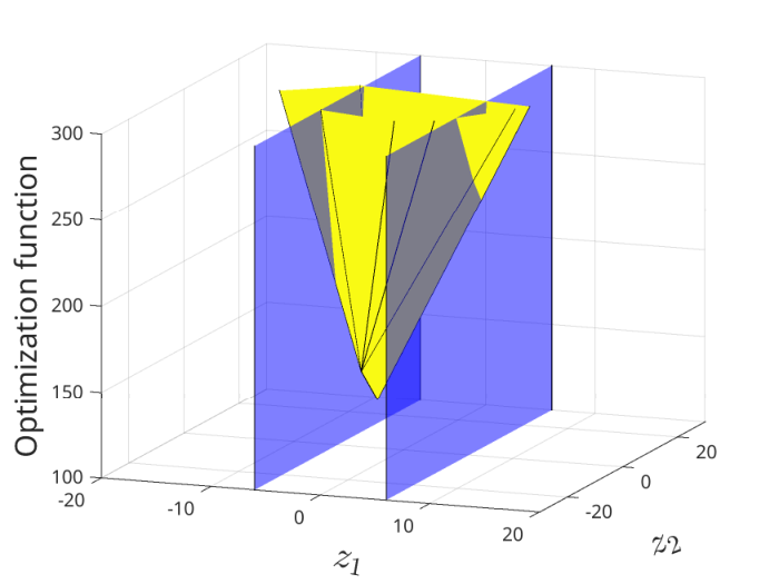
Our randomized approach breaks the problem into sub-problems based on the divide-and-conquer paradigm. Particularly, starting from , it keeps restricting the so-called search interval to smaller ranges denoted as . For example, Figure 6 shows an example where and , specified as the range between the two (blue) planes and 33 3 Recall from Section 2.3 that is the -th coordinate in the dual space, corresponding with the variable .. A vertex would be in the search space if the value of for variable lies within the range . The set of all vertices of that lie within the search interval are called embraced vertices (). At every iteration, the algorithm selects a value to split the search interval in three disjoint intervals - , and . The hyperplane that splits into the three intervals is called the splitting hyperplane, which is defined as .
The choice of during the divide step gives rise to different nature of algorithms. For instance, if the interval were to be divided into three parts based on the mid-value of the range (i.e., ), no matter how fast or accurate the conquer step is designed to be, the approach could only lead to a weakly-polynomial algorithm. Under general positioning assumption, the plane might contain at most one vertex of . Hence, to design a strongly polynomial algorithm, ideally the search interval should be divided in a way that embraced vertices are (almost) split in half. That is, .
Instead of selecting from the continuous range , RandomizedQR uses a vertex from the set of embraced vertices in order to perform the split. I.e., it identifies a vertex for splitting, then uses the value of on A’ as the splitting value (thus ). The challenge, however, is that we would like to identify such that it cuts into two equal halves. Since is in , enumerating for finding is not feasible. We leave the problem of efficiently finding the split point using a deterministic algorithm without enumerating as an open problem. Instead, we draw inspiration from the classical Randomized Quick Sort (RQ-sort) algorithm for identifying the split point. The randomized pivot selection is a key component of RQ-sort to reduce the quadratic worst-case time complexity of quick sort to linearithmic. Applying a similar idea, at a high level, RandomizedQR aims to select the split vertex unformly at random from . The interval is partitioned into three disjoint intervals, and the interval which contains the optimal vertex is identified. Consequently, is updated to the new, smaller interval.
Based on our randomized divide-and-conquer approach, there are two key questions. These questions are addressed in the subsequent sections where we discuss them in detail.
- •
(Divide step) A major difference between RQ-sort and our problem is that, unlike RQ-sort which has random-access to the elements of an array, in our problem is not materialized. As a result, even the exact size of is not known apriori. Hence, it is not possible to (a) directly generate a random index in range and (b) have a random access to a vertex for the generated index. Therefore, a key question is how to efficiently sample (uniformly at random) a vertex from the set of embraced vertices ?
- •
(Conquer step) How to find out which among the 3 intervals contain the optimum vertex?
We design two functions Split and ConstrainedSampling to address these two questions. The role of the ConstrainedSampling function is to sample a vertex uniformly at random from the set of embraced vertices . Split function finds out the interval among the three intervals where the optimum vertex lies. The details of both these functions will be discussed in later-part of this section. The pseudo-code for our approach is presented in Algorithm 4 in Appendix E.
4.2 RandomizedQR in two dimensions
RandomizedQR relies on two key components - Split and ConstrainedSampling. We describe our approaches for both these problems for two dimensions below.
First attempt, a Rejection Sampling approach: In 2D, a vertex is the intersection of a pair of dual lines. Also, following the general positioning assumption, each pair of dual lines intersect exactly once. As a result, in order to draw a uniform random sample from , one can sample one of the dual lines and compute their intersection in constant-time to find the drawn vertex. Therefore, it is straightforward to design a rejection sampling to draw a sample from the set of embraced vertices : (1) sample a pair of dual lines, uniformly at random; (2) compute their intersection point ; (3) accept if , otherwise reject it and try again. This approach, however, is not efficient since the probability of accepting a sample when is as low as . As a result, the expected cost of generating one sample for such regions is .
ConstrainedSampling: Given the inefficiency of the rejection sampling approach, in the following we propose an efficient approach that only generate samples (uniformly at random) that are already in and, hence, no rejection is needed. Our strategy is based on weighted sampling of the dual lines, where the weight of each dual line is the number intersections it has within the search interval . The weights are then used to sample one line. Once a line is sampled, all the vertices of that involve will be enumerated and one of those vertices are returned uniformly at random.
Lemma 3.
ConstrainedSampling is an unbiased sampler for 44 4 The proof is provided in Appendix D.
We still need to find the weight of each dual line , that is, the number of vertices in involving . Consider the vertical line and the order in which the lines intersect with it. The vertical line that is placed at the start (end, resp.) of the interval is termed as start border (end border, resp.). Let this order (top to bottom) in which the lines intersect with the start border be named as start order. Similarly, end order is the order of intersection of the end border with the lines. In Figure 9, the left and right vertical boundary lines in show the start and end borders in that example, while the ordering of dual line intersections with them are the start and end orders. Note that the order of the lines at ( resp.) can be obtained by sorting the slopes of the lines in ascending (descending resp.) order.
Consider the two orderings. Suppose the intersection of the line is blow line on the left line, i.e., , while this ordering is reverse in the right line, i.e., . In this situation the two lines and must intersect somewhere in the search range . Also, the pairs of lines that their ordering do not change in the two lists must not intersect in the search range . As a result, the size of embraced vertices is equal to the number “inversions” in a permutation.
Counting the number of inversions in a permutation is a well-known textbook example for which the divide and conquer algorithm achieves the time complexity of [19].
The Split function: Given the splitting line , the task of Split function is to determine if optimal solution lies on the line , and if not, identify if it is to the left or to the right of the splitting line (i.e. in or ).
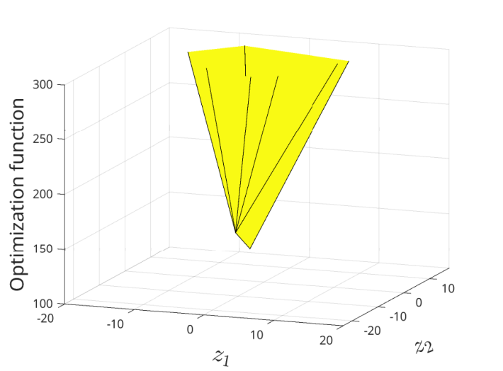
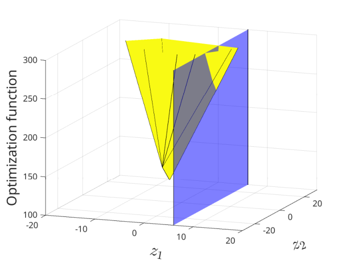
In order to better describe our solution, consider the dual space being augmented by a third dimension, where the third dimension represents the QR optimization function value (e.g., Figure 9). The curve defined in the new space is a convex shape with piece-wise plane faces. The optimization value for the edges that connect the vertices in form the boundaries for these plane faces (e.g., Figure 10). At the vertex where the optimal solution is located, the convex curve (e.g., Figure 9) reaches the least possible value.
The value for variable is used to partition the augmented dual plane into three parts on axis, the half-plane , the line - and the half-plane . The first question to answer is if the optimal solution lies on the splitting-line?
Our design of the Split function for two dimensions relies on the convexity property of the optimization function (Theorem 1). From the theorem, we can deduce that the optimization function is convex within the splitting-plane. Based on convexity, we deploy a divide-and-conquer approach to reach the minima in the plane. The details of our approach are described below.
The vertical splitting plane intersects the dual lines at points in the plane. Recall that the ordering of these intersections is called the split order. As the curve is convex in the plane, the point where the minima is reached must correspond to one of these points. At the minima-point the optimization function score is least within the plane.
At a given point in the split order, the slope of the optimization function can be computed using the optimization scores of the neighboring points. Based on this score, the minima-point has a unique property that both the neighboring points in the split order must have larger optimization values (see Figure 9). Our approach is based on this property that the optimization scores in either direction of the minima-point are monotone and increasing. Note that the slopes on either side keep growing in magnitude but have opposite signs.
Our divide-and-conquer approach uses a binary search with two pointers on either end. The sign of the mid-vertex’s slope is used as a marker to update the two ends. The binary search concludes when we have reached a point where the slope on either side have different signs. The neighborhood of the minima-point can be used to determine if it is the global minima. If all points in the neighborhood have a higher optimization value than the minima-point, then it is a global minima. If not, at least one point in the neighborhood must have a lower optimization value. We use this neighborhood property to determine the optimum interval which contains the optimum point.
Consider the line (lines resp.) that has (have resp.) intersected with the splitting-line at the minima-point. In order to obtain the neighborhood of these points, we compute the intersection of these lines with the remaining dual lines. The intersections (vertices) that are closest to the splitting-line on either side are considered as its neighborhood. If the optimization value of all of these neighborhood points is greater than the minima-point in the plane then minima-point is a global minima. If the current point is not a global minima, then the optimization scores on one side must be strictly greater in any direction. That direction along with the plane are discarded.
The pseudocodes of Split function, BinarySearch2D, and ComputeIntervals are provided in Appendix E, in Algorithms 5, 2, and 3, respectively.
Theorem 4.
The expected time complexity of RandomizedQR in two dimensions is 55 5 The proof is provided in Appendix D.
4.3 Beyond two dimensions
In this section, we extend Split function and ConstrainedSampling to three and higher dimensions.
Split function: Given a hyperplane in dimensions (), the key question that Split function has to answer is: does the (global) optimal solution lie on the splitting-hyperplane? If not, does it lie to left of the splitting-plane or the right?
To answer this question, our approach uses a property that captures the relation between hyperplanes in dimension and dimensional sub-spaces. A hyperplane in dimensions is a sub-space with dimensions. If was 3, then the Split function would want to know the point in the plane where the optimization function is the smallest. But this is exactly the QR problem in two dimensions. Similar observations apply for higher dimensions as well. Hence, as a first step, our solution to the Split function in dimensions can reuse the RandomizedQR algorithm in dimensions to find the optimal solution within the plane.
Once a optimal solution within the dimensional splitting-plane is computed, the next task is to check if it is the global optima. The approach is similar to the two dimensional Split function. The neighborhood of the minima-vertex determines the interval that will be used for the next iteration of RandomizedQR.
Two vertices are neighbors if they share an edge in the skeleton graph . Note that every vertex is formed by intersection of hyperplanes. As edges in are segments of lines in the dimensional space, two neighboring vertices must have hyperplanes in common for them to be incident on an edge. Therefore, to compute the neighborhood of the minima-vertex, the lines that pass through the minima-vertex are computed. Consider a line for this explanation. Each intersection between and the remaining planes gives us a vertex. Among these vertices, the vertices which are closest to the splitting-plane on the left and right gives us the two neighboring vertices for the line . Similarly, the neighbors along each of the lines are computed. There are a total of neighboring vertices.
For each of these vertices, optimization value is computed in linear () time. If the optimization value of the minima-vertex is lower than all these vertices, then it is a global minima. If there is a direction which has a lower optimization score, the hyperplane and the other interval are discarded. The pseudocode of Split for three and higher dimensions is presented in Algorithm 7 in Appendix E.
ConstrainedSampling: The problem of sampling a vertex from the set of embraced vertices in higher dimensions is a much harder problem due to the exponential growth of the number of vertices with dimensions (). Our objective is to achieve a uniform sampling of vertices from the set of embraced vertices . The sampling technique we have devised resembles the approach designed for two dimensions. To obtain a vertex, we must sample a total of hyperplanes. The intersection point is determined through a step-by-step process involving steps. During each step, one of the remaining hyperplanes is sampled based on its respective weight. Therefore, in each step, it is necessary to calculate the weights required for the sampling process.
First step: In the first step, the weight assigned to a hyperplane corresponds to the count of intersections it generates within the range . To provide a clearer understanding of the process, consider a three-dimensional example. When examining the plane , the remaining planes are represented as lines (typically referred to as dimensional objects). A simple observation is that any intersection that involves a plane must occur within the range on that plane. For example, say planes , and intersected to form a vertex within the search interval . This intersection vertex must lie on all three planes , and . Counting the number of Intersections on a plane has already been studied in the two dimensional ConstrainedSampling approach. Therefore, to determine the count of intersections a plane has within the range in three dimensions, the two-dimensional ConstrainedSampling method is utilized with the appropriate parameters.
In general dimensional space, the dimensional hyperplanes are dimensional sub-spaces. As observed in the example of three-dimensional space, if a hyperplane has an intersection within the range , it must be located somewhere on . Hence, we can invoke the ConstrainedSampling in dimensional space. Whenever an intersection occurs, the counts of all the hyperplanes that have been a part of the intersection are incremented by one.
Our approach for ConstrainedSampling in dimensions goes over each hyperplane and accounts for the intersections that happens on each hyperplane. Once all the intersections for a particular hyperplane have been considered, is eliminated from the set of planes and is no longer taken into account for subsequent intersections. At the end of this process, all the hyperplanes are updated with their respective intersections counts. Based on these counts the first hyperplane is sampled.
Second and later steps: The process of sampling the next hyperplane follows a similar procedure. In step , hyperplanes have already been sampled. The intersection of the sampled hyperplanes forms a dimensional sub-space. There are a total of hyperplanes left to sample from. ConstrainedSampling from the dimensions is used in a similar manner as the first step.
The process of sampling these hyperplanes continues until all the hyperplanes are sampled. This pseudo code is presented in Algorithm 6 in Appendix E.
Theorem 5.
The expected time complexity of our RandomizedQR algorithm in higher dimensions () is 66 6 The proof is provided in Appendix D.
5 Final remarks
In this paper, we studied the Quantile Linear Regression problem in two and higher dimensions. Our first contribution is the UpdateNeighbor subroutine which helps us update the optimization function efficiently () while navigating the neighboring vertices (intersection points) in dual space. We propose two strongly polynomial approaches to solve the QR problem. The -set based approach is a parameter sensitive algorithm that enumerates the level of the arrangement while using the UpdateNeighbor subroutine to compute the optimization functions values. We prove that its time complexity is better than all known approaches for two dimensions. The problem of efficient enumeration of -sets in higher dimensions is an open problem which can improve our time complexity our higher dimensions. Our second approach - RandomizedQR, is a randomized divide-and-conquer approach to the QR problem which splits the dimensional arrangement into disjoint half-spaces and determining the half-space that contains the optimal solution. RandomizedQR is also proved to be more efficient than all existing approaches for and dimensions including weakly polynomial approaches. RandomizedQR is faster than all existing strongly-polynomial approaches. The problem of designing a deterministic algorithm that efficiently finding a hyperplane in dimensions such that it splits the vertices in embraced vertices into two “equal” parts is an interesting open problem for future work.
Appendix
Appendix A Quantile Regression: Challenges, and State of Art
Linear Regression is a seminal approach in statistics and machine learning, used for building linear predictive models between a response (i.e., dependent) variable and one or more predictor (i.e., independent) variables. Linear regression is over two centuries old (dating back to Legendre and Gauss) and is often considered as the forerunner of modern machine learning [24]. We revisit two classical linear regression techniques: Ordinary Least Square Regression (OLS) and Quantile Regression (QR). Both build linear models but with different objective functions: in OLS, the objective is to minimize the mean squared error (i.e., norm) between the dependent variable and that predicted by the model; whereas in QR, the objective is to minimize the mean absolute error (i.e., norm).
Why Quantile Regression? Historically, OLS has been much more widely used than QR. This is primarily because (as we will discuss shortly) QR is plagued by unacceptably high computational resource needs, whereas there exist extremely resource-efficient and scalable algorithms for building OLS models.
Nevertheless, despite its computational advantages, OLS has a major limitation: OLS is not a robust model. It can be easily skewed in the presence of outliers in the data, which makes OLS a poor model of choice in several emerging applications where the robustness of the predictive model is critically needed. On the other hand, QR is a robust model. In simple terms, the comparison of OLS and QR is analogous to the “mean versus median” comparison mentioned above. That is why QR is considered for applications where model robustness in the presence of outliers and skew in the data is critically needed, such as healthcare [23], ecology [3], and others [8]. Beyond robustness, another attraction of quantile regression is that it is advantageous when conditional quantile functions are of interest, which has application in uncertainty quantification and conformal prediction in AI systems as well as approximate query processing in databases [26, 25]. In fact, if the scalability and computational efficiency of QR could be significantly improved, its applicability would increase dramatically across an even more broad range of applications [3].
Computational Challenges of Quantile Regression: The computational challenges of QR are best highlighted by the following observations. Consider a database with points and attributes, of which one attribute is the response (i.e., independent) variable, and the rest are predictor (i.e., dependent) variables. Typically in most data fitting problems. For OLS, since the objective function to be minimized (least square) is quadratic and differentiable, this yields a highly scalable training algorithm with time complexity of time, and space complexity of [6]. Note that the time complexity is effectively linear in for bounded dimensions. In contrast, the objective function in quantile regression is defined by the norm, i.e., sum of the absolute error, which has “piecewise linear” characteristics.
Hence, its optimization is much more challenging. The state-of-the-art approach for QR [24] applies a reparametrization technique to convert the problem into a huge linear programming formulation involving linear constraints and variables. Solving these linear programs require significantly more resources (time and memory) compared to OLS [24], making QR prohibitive for all but small-to-moderate sized datasets. This need for extensive computational resources has been one of the main reasons for the relative lack of adoption of QR in emerging Big Data applications.
State of Art Techniques and Tools: Quantile Regression is a well-studied research problem. In the appendix (Section B), we provide a more detailed overview of the literature, but highlight a few key works here.
Two prominent classes of exact techniques to solve the QR problem are exterior-point based [1] and interior-point based [24] approaches. Barrodale and Robert (BR) proposed a simplex-based exterior point technique [1], which moves from one exterior point (i.e., a “corner” of the feasible polytope defined by the linear program) to another exterior point, in the direction of steepest gradient descent. The core idea of BR originates from Edgeworth’s bi-variate weighted median based 1888 approach [13]. The run time of this algorithm is , which is still the state of the art algorithm for two dimensions (i.e., ). All the exterior points based approaches are only suitable for small problem instances with around points and few attributes [24]. Portnoy and Koenkar later proposed a primal-dual interior point method (IPM) which finds the optimal solution by minimizing the difference between primal and dual objective cost [24]. This method is reasonably fast for larger input sizes in practice, but worst-case theoretical runtime complexity is where is the desired accuracy [29]. Moreover, BR and IPM are extremely memory hungry, hence not suitable for big data problem instances under resource constraints.
Appendix B Related work and discussion on state of the art
The idea of quantile regression was introduced even before OLS regression. Around 1757, Boscovich proposed the idea of fitting a line for 2-dimensional data by minimizing the sum of absolute residuals under the assumption of mean of residuals has to be zero. Laplace gave an algebraic formulation of the problem in his Methode de Situation in 1789. In 1809 Gauss suggested to remove zero mean residual constraint. Later in 1823, he also proposed least square criterion (i.e., OLS). As OLS has more analytical and computational simplicity, it has been always popular. However, a criterion is a choice and there are different cases where one criterion will outperform others. In 1888, Edgeworth proposed a geometry based solution for the bi-variate median regression problem [2].
In the 20th century, there has been extensive work on quantile regression which helped a wide range of applications. In 1974, Barrodale and Roberts [1] used simplex technique to solve median regression problem as a bounded dual problem. Bloomfield and Steiger [2] explored the simplex technique for median regression in depth and suggested exploring a normalized steepest edge direction instead of steepest edge direction.
Before 1987, all the quantile regression techniques were focusing on median regression Koenker and d’Orey [21] generalized the criterion for any quantile which is now known as quantile regression. In median regression, an input point incurs a cost of absolute deviation. For quantile regression parameter , Koenker and d’Orey proposed to assign and weight to negative and positive residuals. After the development of generalized quantile regression, there has been an extensive research in this area. We mention a few prominent work in this paper. The primary focus has been on the development of faster quantile regression algorithms [7]. Another research direction is finding quantile regression for multiple quantiles [24, 7]. In 1997, Portnoy and Koenker [24] developed a primal dual interior point method where in each step the goal is to minimize the different between primal dual objective loss. It is extremely fast compared to the all previous methods.
In the continuous quest for faster quantile regression, either the objective criterion has often been modified [7, 30] or approximations [22, 14, 31] have been introduced . As none of these are widely accepted, we only consider the original quantile regression problem in this paper. If we we consider the entire history of quantile regression, the most prominent two exact techniques are based on Barrodale and Roberts[1], and Portnoy and Koenkar [24]. The latest updated implementation based on these techniques can be found in quantreg package [16] in the R library, maintained by Roger Koenkar which is a gold standard public library for quantile regression. However, these widely used and accepted implementations are quite memory hungry. Moreover, the run time complexity of these implementations are still far behind to tackle the challenges of modern big data applications. So it is extremely important to develop techniques that can overcome these ever increasing challenges.
B.1 Existing State-of-Art Exact Approaches
In this subsection, we describe a few properties of QR, connection to linear programming, and existing exact techniques to solve problem.
There has been extensive research conducted on QR over the last two hundred years [2]. Wagner [28] identified the connection between linear programming and -regression. A reparameterization technique[20] is used to convert the QR problem into a linear programming problem. The linear constraints of a linear programming problem create a convex polytope. Solutions to the QR problem are based on utilizing the exterior (corner) points or interior points of this convex polytope.
We give a brief overview of prior algorithms for QR. The focus of QR research has been primarily on how to make the algorithms faster, with the eventual goal of trying to make it an alternative to OLS regression. There have been two broad categories of techniques, exact techniques (where the objective function is minimized) and approximate/heuristic techniques. There is a wide body of techniques that belong to the latter category, e.g., modifying the original objective function to achieve a faster performance [7, 30], as well as other approximation approaches [22, 14, 31]. However, since our focus in this paper is to consider regression as a robust and trustworthy technique, we are only interested in exact approaches.
Prior research on exact quantile regression techniques can be divided into two categories: exterior point based approaches and interior point based approaches. In 1888, Edgeworth designed an exterior point approach [13] to solve 2-dimensional -regression. A modern implementation of Edgeworth’s technique that utilizes a linear-time weighted median finding algorithm as subroutine can solve 2-dimensional QR in time. Barrodale and Roberts (BR) [1] designed a simplex algorithm-based approach for any dimension that starts from an exterior point and moves in the direction of the steepest gradient descent of the objective function. This algorithm runs in time for 2-dimensional QR. However, these types of approaches are not very scalable for large datasets.
Portnoy and Koenkar [24] introduced a primal-dual interior point method (IPM) solution for QR. In this approach, the QR problem is solved using primal and dual space both simultaneously. IPM adds a barrier function in the objective function, which helps explore the the solutions in interior points. The algorithm stops when the primal and dual objective difference is smaller than a given small threshold . The worst case run time complexity for IPM is [29]. Although IPM is most widely used QR technique in practice, it is not yet ready to handle big data.
The detailed related works can be found in Appendix B.
Appendix C Details of k-set based two dimensional QR problem
C.1 QR2D-Neighbor-Baseline: Algorithm Based on Neighbor Exploration
In this subsection, we introduce QR2D-Neighbor-Baseline algorithm that utilizes the UpdateNeighbor subroutine.
Exploring the vertices in the complete skeleton graph presents us with an interesting algorithm to obtain the optimal QR line. Let us consider for simplicity that a GetNeighbors oracle exists that can quickly provide us with the neighbors of a given vertex. We can start from any of the vertices and explore neighboring vertices around it in a Breadth First Search (BFS) manner while updating the aggregate entities and objective cost. While for simplicity of understanding, we choose BFS for exploration, it does not change the analysis that follows. We stop when no new neighboring vertices with a lower optimization value are found. The optimal QR hyperplane is the vertex with the smallest optimization function among the explored intersection points.
Note that a naive way to build a GetNeighbors Oracle is to compute the vertices of the complete skeleton graph beforehand. Computing and storing intersection points consumes space and time. Often the space is prohibitive in practice. As the dimensions grow beyond , this neighborhood-based approach is prohibitive as there are a total of points. Exploring these intersection points is far more expensive than the IPM for larger dimensions.
This algorithm provides an approach that explores the neighbors of vertices until it reaches the optimal solution. While this approach produces a similar complexity as the exterior point method for two dimensions, it creates an intuition for our optimized 2D algorithm. We present a more efficient approach for two dimensions later in this section.
C.2 QR2D-k-Set-Baseline: -Set Based Algorithm
In this subsection, we introduce QR2D-k-Set-Baseline algorithm that utilizes the computational geometry concept of -set.
Recall from Section 2.3 that a -set is a subset containing points that can be separated from the rest of the points by a hyperplane. -sets have often been used in various computational geometry settings to solve numerous problems.
An interesting observation that can be made on the optimal solution QR hyperplane is that it separates the points into and points [24]. While there are many hyperplanes that separate points into two parts (with and points), we are interested in the specific hyperplane that provides the lowest optimization score. As -sets separate the points into and points, the optimal hyperplane must be one of the -set separating hyperplanes such that . The enumeration of all -sets can also be viewed as a walk along the -level of an arrangement. Hence, the optimal hyperplane can be found along the vertices encountered during the walk on the -level of the arrangement.
The QR problem in 2 dimensions can utilize this property (the result of Theorem 2). The optimal hyperplane in primal space is represented by a point in dual space. This point is one of the vertices in the complete skeleton graph corresponding to the -level arrangement in the dual space. One approach to solving this problem would be to enumerate the vertices corresponding to the -level of the arrangement and, for each vertex, compute the value of the optimization function.
We first present QR2D-k-Set-Baseline algorithm that makes use of the concept of -sets without the use of aggregate entities to solve the problem. This approach has to compute the value (error) of the optimization function for a vertex that corresponds to a dual point in the -level arrangement. Computing the optimization function for each of these vertices involves aggregating the error contribution of each of the points in the primal space using the line . Note that each of the computations consumes time. For each of the vertices corresponding to the dual points in the -level arrangement, the naive error computation is repeated, and the optimal line corresponds to that line with the least error.
Time complexity: For a given vertex in the -level arrangement, a naive approach to compute the error without making use of UpdateNeighbor subroutine takes a total of time. The upper bound on the intersection points in -level of an arrangement is bounded by . Hence, the total time taken for the naive approach is for a given (). As when , the worst case time complexity is .
C.3 Illustration of UpdateNeighbor subroutine
In this subsection, we illustrate how we can reduce the computational cost while moving from one vertex to a neighboring vertex of the complete skeleton of the arrangement by maintaining only a few aggregate values. For this illustration of UpdateNeighbor subroutine, we use our running example from Table 3 with .

As explained in Section 2, a vertex in the complete skeleton graph (point in dual space) refers to a QR hyperplane in primal space. The optimal solution lies in one of these vertices in the complete skeleton graph. Let be a complete skeleton graph constructed from Figure 4 and be any vertex constructed from the intersection of dual line and . and are neighbors in the arrangement which will be used in our illustration. Figure 11 shows the primal representation of and where each represents a line. From the definition of residual set in Section 2, and for . We calculate the sum along -axis and -axis for these two group of points and call these aggregate values at . Given these aggregate values for , we would like to answer the following questions as steps of our demonstration: (i) How to calculate the objective values at ? (ii) How to calculate the aggregate values at from in ? and (iii) If aggregate values are known for , how to calculate the objective value at ?
As shown in Figure 11, passes through input points and in primal space and its parameter vector is . For all , let , be the sum along X and Y axis respectively. Similarly, for all , let , and be the sum along X and Y axis respectively. Given the aggregate values for , the objective cost at can be calculated using following process.
Now, we will try to answer how we will update the aggregate values at from . As shown in Figure 11, only one input point changes its residual sign from positive to negative in to transition. For , and . If we want to calculate the aggregate values at from , the information of input point can be utilized in the following fashion.
Earlier, we have shown how to calculate objective cost from aggregate values at . Similarly, the objective cost for can be calculated using the aggregate values. If the aggregate values at are known, the aggregate values and objective cost at can be calculated in time and space. Although our illustration is in 2-dimension, our UpdateNeighbor subroutine works in any dimension.
Appendix D Proofs of Theorems and Lemmas
Theorem 3. Given the aggregate values , , , for a vertex in the complete skeleton graph, the aggregate values can be updated in time when we move to a neighboring vertex.
Proof.
Any vertex in the complete skeleton graph represents a hyperplane in the primal space which divides the set of points in into two sets, and . When we move from a vertex to its neighboring vertex, the sets and change in one of three ways,
- •
A point in primal space moves from above the hyperplane to below the hyperplane i.e., a point moves from to .
- •
A point in primal space moves from below the hyperplane to above the hyperplane i.e., a point moves from to .
- •
The hyperplane moves such that a point from above is exchanged with a point from below. In such a case, the number of points above the hyperplane remains the same, i.e., a point from is swapped with a point in . Note that the in this case may not be .
For each of the three cases, we prove that the aggregate values can be updated in time. For the rest of this proof, let the new sets after the update be represented by and .
Let us consider the first case, where the hyperplane moves such that a point moves from the set to , i.e., a point in primal space which was above the hyperplane (vertex) now lies below the neighboring hyperplane (neighbor vertex). Let be the point that is involved in the transition. As we know the details of point , we can remove the contribution of towards and add the contribution to aggregates entities of . The formulae for the update are as below,
As there are equations, each of which takes time to update, the total time taken to update the aggregate values is .
The second case, where a point in primal space has moved from below the hyperplane (vertex) to above the neighboring hyperplane (neighbor vertex), can be updated similarly. Let be the point that is involved in the transition. The formulae for the update operation for the second case are,
With equations, each of which take the overall time complexity is time.
Let us consider the third case, where the hyperplane moves such that a point from above is exchanged with a point from below. In this case, a point from is swapped with a point in . Let be the point that is moved from to , and be the point moved from to . As we know the details of points and , we can remove the contribution of towards and add the contribution of to it. We perform vice verse operation to . The formulae for the update are as below,
With a total of equations, each of which take , the overall time complexity is time. Hence, proved. ∎
Lemma 1. QReg2D has a time complexity of , where is an arbitrarily small constant.
Proof.
For the first -set obtained through the enumeration, the optimization function and aggregate values need to be calculated by a linear scan over the points which takes time. Updating the optimization function value and aggregate values as we explore neighboring -set takes time. The points in the -level of the arrangement can be computed using a sweep Line algorithm [12, 5, 4] in where is the number of -set and is an arbitrarily small constant. The upper bound on total number of -sets is given by Dey [9], . This brings the overall time taken to . As is a percentage of , the overall time complexity . Hence, proved. ∎
Proof.
This proof follows along similar lines to the proof of Lemma 1. However, if we use a randomized incremental algorithm instead of the deterministic algorithm, the enumeration can be done in expected time (Corollary 4.4 [4]). The points in the -level of the arrangement can be computed using Randomized Incremental algorithm[4] in time (Corollary 4.4). This brings the overall time taken to . ∎
Lemma 3. ConstrainedSampling is an unbiased sampler for .
Proof.
Let be the number of intersections in that involve . The probability of selecting each line is
After selecting a line , the probability that a specific intersection involving it is . Now, for an intersection , let and be the dual lines that involve it. The probability of sampling is
∎
Theorem 4 The expected time complexity of RandomizedQR in two dimensions is .
Proof.
RandomizedQR algorithm relies on two important functions - Split function and ConstrainedSampling. For this proof, we first analyze the running time of these two approaches and in a final step use these to prove the run time of RandomizedQR.
Split function time complexity: The Split function for two dimensions has two main parts (i) Binary Search routine, (ii) Update . The binary search routine starts from an array of intersections with length . In each step, the optimization function value is computed for the mid-point, which consumes linear time (). As binary search finds the answer in steps, the total time consumed by the binary search is .
Once the optimum in the plane is computed, the intersections of the corresponding dual line with other lines are obtained in linear time. Computing the optimization value for the neighboring intersections can be performed in () time. Thus the total time complexity of Split function is .
Time complexity of ConstrainedSampling: The first step in the weighted sampling strategy is to determine the weights of the dual lines. Our approach internally uses the inversion counting problem to obtain the weights. The inversion counting problem is well known, and runs in time . These weights are then used to sample the first dual line. In linear time, the intersections of the sampled line with all the other lines are obtained. One of these lines that satisfy is sampled. Thus, the time complexity is dominated by the inversion counting problem.
The sum of the time complexities of the divide and conquer steps of our algorithm is . Let the time taken by this single divide-and-conquer step be denoted entity by (where represents the number of dimensions).
Our proof follows along similar lines as the Randomized Quick-Sort algorithm. Let the interval contain vertices of . The recurrence for our problem is given below,
where represents the removal of vertices from the range. Assume that the (i.e. ). Note that one of the recursive calls consumes time as it corresponds to the optimal hyperplane.
By choosing the right value for constants and , the above inequality can be satisfied. Thus, the expected run-time of our RandomizedQR approach is = .
∎
Theorem 5 The expected time complexity of our RandomizedQR algorithm in higher dimensions () is .
Proof.
RandomizedQR algorithm depends on Split function and ConstrainedSampling. We explore the time complexity analysis of these two methods before the analyze the RandomizedQR function in dimensions. For this proof let denote the time complexity of RandomizedQR function in dimensions, where is the number of vertices in . Note that all the terms used in this proof are in expected time.
Split function: The Split function in dimensions calls the dimensional RandomizedQR function. Additionally, the hyperplanes are used to obtain neighboring intersections (vertices). Each of the hyperplanes gives us a line in the dimensional space. Each of these lines is then used to compute the intersections (vertices) with the remaining planes. The total time complexity to compute the intersections is . Additionally, the optimization value for each of the neighboring vertices is computed. As each computation consumes time, the total time taken for these computations is . Hence, the total time complexity of Split function is .
ConstrainedSampling: The ConstrainedSampling function uses recursive lower dimensional ConstrainedSampling calls to obtain the weights of each hyperplane. Using these weights the first hyperplane is sampled. Then recursive calls are made to dimensional ConstrainedSampling calls to obtain the weights of each hyperplane. The process of obtaining weights and sampling continues until hyperplanes are sampled which intersect at a vertex inside . Let represent the time complexity of ConstrainedSampling in dimensions (). The recursive calls made by ConstrainedSampling in dimensions can be captured with the equation . For two dimensions, the time complexity of ConstrainedSampling is .
But we know that
Using the above expression we get,
For three dimensions, using the above equation we get . In dimensions, we get .
As the divide-and-conquer steps are performed in succession, let us consider a term which is the sum of the time complexities of these two functions. Let denote the term that corresponds to the sum of these two functions.
Similar to the proof for two dimensions, we use be the vertices in . Let be the time complexity of RandomizedQR in dimensions.
Assume that each call consumes time.
Note that the expectation of a product of random variables is the product of the expectation of the two random variables. Similar to the proof for two dimensions, by choosing right constants for and we can satisfy the above inequality. The overall time complexity can be written in the form,
The equation for dimension gives us . Similarly, for general , the term grows at a faster rate compared to . Hence the overall complexity is ∎
Appendix E Pseudocodes
References
- Barrodale and Roberts [1973] Ian Barrodale and Frank DK Roberts. An improved algorithm for discrete linear approximation. SIAM Journal on Numerical Analysis, 10(5):839–848, 1973.
- Bloomfield and Steiger [1983] Peter Bloomfield and William L Steiger. Least absolute deviations: theory, applications, and algorithms. Springer, 1983.
- Cade and Noon [2003] Brian S Cade and Barry R Noon. A gentle introduction to quantile regression for ecologists. Frontiers in Ecology and the Environment, 1(8):412–420, 2003.
- Chan [1999] Timothy M Chan. Remarks on k-level algorithms in the plane, 1999.
- Chan [2001] Timothy M Chan. Dynamic planar convex hull operations in near-logarithmic amortized time. Journal of the ACM (JACM), 48(1):1–12, 2001.
- Chernick [2002] Michael R Chernick. The elements of statistical learning: Data mining, inference and prediction, 2002.
- Chernozhukov et al. [2020] Victor Chernozhukov, Iván Fernández-Val, and Blaise Melly. Fast algorithms for the quantile regression process. Empirical economics, pages 1–27, 2020.
- Davino et al. [2013] Cristina Davino, Marilena Furno, and Domenico Vistocco. Quantile regression: theory and applications, volume 988. John Wiley & Sons, 2013.
- Dey [1997] Tamal K Dey. Improved bounds on planar k-sets and k-levels. In Proceedings 38th Annual Symposium on Foundations of Computer Science, pages 156–161. IEEE, 1997.
- Deza et al. [2008] Antoine Deza, Eissa Nematollahi, and Tamás Terlaky. How good are interior point methods? klee–minty cubes tighten iteration-complexity bounds. Mathematical Programming, 113(1):1–14, 2008.
- Edelsbrunner [1987] Herbert Edelsbrunner. Algorithms in combinatorial geometry, volume 10. Springer Science & Business Media, 1987.
- Edelsbrunner and Welzl [1986] Herbert Edelsbrunner and Emo Welzl. Constructing belts in two-dimensional arrangements with applications. SIAM Journal on Computing, 15(1):271–284, 1986.
- Edgeworth [1888] Francis Ysidro Edgeworth. Xxii. on a new method of reducing observations relating to several quantities. The London, Edinburgh, and Dublin Philosophical Magazine and Journal of Science, 25(154):184–191, 1888.
- Feng et al. [2015] Yang Feng, Yuguo Chen, and Xuming He. Bayesian quantile regression with approximate likelihood. Bernoulli, 21(2):832–850, 2015.
- Haupt et al. [2014] Harry Haupt, Friedrich Lösel, and Mark Stemmler. Quantile regression analysis and other alternatives to ordinary least squares regression. Methodology, 2014.
- [16] https://cran.r project.org/web/packages/quantreg/index.html.
- Jiang et al. [2020] Shunhua Jiang, Zhao Song, Omri Weinstein, and Hengjie Zhang. Faster dynamic matrix inverse for faster lps. arXiv preprint arXiv:2004.07470, 2020.
- John and Nduka [2009] Onyedikachi O John and Ethelbert C Nduka. Quantile regression analysis as a robust alternative to ordinary least squares. Scientia Africana, 8(2):61–65, 2009.
- Kleinberg and Tardos [2006] Jon Kleinberg and Eva Tardos. Algorithm design. Pearson Education India, 2006.
- Koenker and Bassett Jr [1978] Roger Koenker and Gilbert Bassett Jr. Regression quantiles. Econometrica: journal of the Econometric Society, pages 33–50, 1978.
- Koenker and d’Orey [1987] Roger W Koenker and Vasco d’Orey. Algorithm as 229: Computing regression quantiles. Applied statistics, pages 383–393, 1987.
- Meinshausen and Ridgeway [2006] Nicolai Meinshausen and Greg Ridgeway. Quantile regression forests. Journal of machine learning research, 7(6), 2006.
- Olsen et al. [2017] Margaret A Olsen, Fang Tian, Anna E Wallace, Katelin B Nickel, David K Warren, Victoria J Fraser, Nandini Selvam, and Barton H Hamilton. Use of quantile regression to determine the impact on total health care costs of surgical site infections following common ambulatory procedures. Annals of surgery, 265(2):331, 2017.
- Portnoy and Koenker [1997] Stephen Portnoy and Roger Koenker. The gaussian hare and the laplacian tortoise: computability of squared-error versus absolute-error estimators. Statistical Science, 12(4):279–300, 1997.
- Savva et al. [2020] Fotis Savva, Christos Anagnostopoulos, and Peter Triantafillou. Ml-aqp: Query-driven approximate query processing based on machine learning. arXiv preprint arXiv:2003.06613, 2020.
- Thirumuruganathan et al. [2022] Saravanan Thirumuruganathan, Suraj Shetiya, Nick Koudas, and Gautam Das. Prediction intervals for learned cardinality estimation: An experimental evaluation. In 2022 IEEE 38th International Conference on Data Engineering (ICDE), pages 3051–3064. IEEE, 2022.
- Vaidya [1989] Pravin M Vaidya. Speeding-up linear programming using fast matrix multiplication. In 30th annual symposium on foundations of computer science, pages 332–337. IEEE Computer Society, 1989.
- Wagner [1959] Harvey M Wagner. Linear programming techniques for regression analysis. Journal of the American Statistical Association, 54(285):206–212, 1959.
- Wright [1997] Stephen J Wright. Primal-dual interior-point methods. SIAM, 1997.
- Yang et al. [2013] Jiyan Yang, Xiangrui Meng, and Michael Mahoney. Quantile regression for large-scale applications. In International Conference on Machine Learning, pages 881–887. PMLR, 2013.
- Zheng [2011] Songfeng Zheng. Gradient descent algorithms for quantile regression with smooth approximation. International Journal of Machine Learning and Cybernetics, 2(3):191–207, 2011.