Artificial Intelligence for Science in Quantum, Atomistic, and Continuum Systems
Abstract.
Advances in artificial intelligence (AI) are fueling a new paradigm of discoveries in natural sciences. Today, AI has started to advance natural sciences by improving, accelerating, and enabling our understanding of natural phenomena at a wide range of spatial and temporal scales, giving rise to a new area of research known as AI for science (AI4Science). Being an emerging research paradigm, AI4Science is unique in that it is an enormous and highly interdisciplinary area. Thus, a unified and technical treatment of this field is needed yet challenging. This work aims to provide a technically thorough account of a subarea of AI4Science; namely, AI for quantum, atomistic, and continuum systems. These areas aim at understanding the physical world from the subatomic (wavefunctions and electron density), atomic (molecules, proteins, materials, and interactions), to macro (fluids, climate, and subsurface) scales and form an important subarea of AI4Science. A unique advantage of focusing on these areas is that they largely share a common set of challenges, thereby allowing a unified and foundational treatment. A key common challenge is how to capture physics first principles, especially symmetries, in natural systems by deep learning methods. We provide an in-depth yet intuitive account of techniques to achieve equivariance to symmetry transformations. We also discuss other common technical challenges, including explainability, out-of-distribution generalization, knowledge transfer with foundation and large language models, and uncertainty quantification. To facilitate learning and education, we provide categorized lists of resources that we found to be useful. We strive to be thorough and unified and hope this initial effort may trigger more community interests and efforts to further advance AI4Science.
1. Introduction
Decades of artificial intelligence (AI) research has culminated in the renaissance of neural networks (LeCun et al. 1998) under the name of deep learning. Since AlexNet (Krizhevsky et al. 2012), a decade of intensive research has led to many breakthroughs in deep learning, including, for example, ResNet (He et al. 2016), diffusion and score-based models (Ho et al. 2020; Song et al. 2020), attention, transformers (Vaswani et al. 2017), and recently large language models (LLM) and ChatGPT (OpenAI 2023), etc. These developments have led to continuously improved performance for deep models. When coupled with growing computing power and large-scale datasets, deep learning methods are becoming dominant approaches in various fields, such as computer vision and natural language processing. Propelled by these advances, AI has started to advance natural sciences by improving, accelerating, and enabling our understanding of natural phenomena at a wide range of spatial and temporal scales, giving rise to a new area of research, known as AI for science. It is our belief that AI for science opens a door for a new paradigm of scientific discovery and represents one of the most exciting areas of interdisciplinary research and innovation.
Historically, the importance of computing in accelerating discoveries in natural sciences has been noted. Almost one hundred years ago in 1929, the quantum physicist Paul Dirac stated that “The underlying physical laws necessary for the mathematical theory of a large part of physics and the whole of chemistry are thus completely known, and the difficulty is only that the exact application of these laws leads to equations much too complicated to be soluble.” (Dirac 1929) In quantum physics, it is known that the Schrödinger’s equation provides precise descriptions of behaviors of quantum systems, but solving such an equation is only possible for very small systems due to its exponential complexity. In fluid mechanics, the Navier-Stokes equations describe spatiotemporal dynamics of fluid flows, but solving these equations of practically useful sizes is highly demanding, especially when computing efficiency is also required. Similar to these two examples, the underlying physics of many natural science problems are known and can be described by a set of mathematical equations. The key difficulty lies in how to solve these equations accurately and efficiently. Recent studies have shown that deep learning methods can accelerate the computing of solutions for these equations. For example, deep learning methods have been used to compute the solutions of Schrödinger’s equation in quantum physics (Carleo and Troyer 2017; Pfau et al. 2020; Hermann et al. 2020; Hermann et al. 2023) and Navier-Stokes equations in fluid mechanics (Kochkov et al. 2021b; Brunton et al. 2020). In these areas, simulators are employed to compute solutions of mathematical equations, and the results are used as data to train deep learning models. Once trained, these models can make predictions at a speed that is much faster than simulators. In addition to improved efficiency, deep learning models have been shown to exhibit better out-of-distribution (OOD) generalization, with scope extended to much wider practical settings, where training and unseen data usually follow different distributions.
In other areas such as biology, the underlying biophysical process is not completely understood and may not ultimately be described by mathematical equations. In these cases, experimentally generated data can be used to train deep learning models in order to model the underlying biophysical process. For example, in biology, AI systems, such as AlphaFold (Jumper et al. 2021), RoseTTAFold (Baek et al. 2021), and ESMFold (Lin et al. 2023a), trained on experimentally acquired 3D structures, enable the computational prediction of protein 3D structures at an accuracy comparable to experimental results. In addition to technical challenges, a key element in these areas is the availability of large amounts of experimentally generated data. For example, the success of AlphaFold, RoseTTAFold, and ESMFold highly relies on the large amount of protein 3D structure data generated using experiments and deposited into databases, such as the Protein Data Bank.

1.1. Scientific Areas
In this work, we provide a technical and unified review of several research areas in AI for science that researchers have been working on during the past several years. We organize different areas of AI for science by the spatial and temporal scales at which the physical world is modeled. An overview of scientific areas we focus in this work is given in Figure 1.
Quantum Mechanics studies physical phenomena at the smallest length scales using wavefunctions, which describe the complete dynamics of quantum systems. In quantum physics, wavefunctions are obtained by solving the Schrödinger equation, which incurs exponential complexity. In this work, we provide technical reviews on how to design advanced deep learning methods for learning neural wavefunctions efficiently. For a comprehensive review of machine learning in quantum science, one may refer to (Dawid et al. 2022).
Density Functional Theory (DFT) and ab initio quantum chemistry approaches are first-principles methods widely used in practice to calculate electronic structures and physical properties of molecules and materials. However, these methods are still computationally expensive, limiting their use in small systems (1,000 atoms). In this work, we present technical reviews on deep learning methods for accurately predicting quantum tensors, which in turn can be used to derive many other physical and chemical properties, including, electronic, mechanical, optical, magnetic, and catalytic properties of molecules and solids. We also touch on machine learning methods for density functional learning.
Small Molecules, also known as micromolecules, typically have tens to hundreds of atoms and play important regulatory and signaling roles in many chemical and biological processes. For example, 90% of approved drugs are small molecules, which can interact with target macromolecules (like proteins), altering the activity or function of the target. In recent years, significant progress has been made in using machine learning methods to accelerate scientific discoveries on small molecules at the atomistic level. In this work, we present in-depth technical reviews on small molecule representation learning, molecular generation, simulation, and dynamics.
Proteins are macromolecules that consist of one or more chains of amino acids. It is commonly believed that amino acid sequences determine protein structures, which in turn determines their functions. Proteins perform most of the biological functions, which include structural, catalytic, reproductive, metabolic, and transporting roles, etc. Recently, machine learning approaches have led to dramatic advances in protein structure prediction (Jumper et al. 2021; Baek et al. 2021; Lin et al. 2023a). In this work, we provide technical reviews on how to learn representations from protein 3D structures, and how to generate and design novel proteins.
Materials Science studies the relationship of processing, structure, properties, and performance of materials. The intrinsic structure of materials from atomistic, to micro and continuum scale determine their quantum, electronic, catalytic, mechanical, optical, magnetic, and other properties through interplay with external stimuli/environment. Recently, machine learning methods have been developed to predict the properties of crystal materials and design novel crystal structures. In this work, we provide technical reviews on the property prediction and structure generation of crystal materials.
Molecular Interactions study how molecules interact with each other to carry out many of the physical and biological functions. Recent advances in machine learning have spurred the renaissance in modeling various molecular interactions, such as ligand-receptor and molecule-material interactions. In this work, we present in-depth and comprehensive reviews on such advances.
Continuum Mechanics models physical processes that evolve in time and space at the macroscopic level using partial differential equations (PDEs), including fluid flows, heat transfer, and electromagnetic waves, etc. However, solving PDEs using classic solvers suffers from several limitations, including low efficiency, difficulties in out-of-distribution generalization and multi-resolution analysis. In this work, we provide reviews on recent deep learning methods for surrogate modeling that addresses these limitations.
In each area, we provide a precise problem setup and discuss the key challenges of using AI to solve such problems. We then provide a survey of major approaches that have been developed. We also describe datasets and benchmarks that have been used to evaluate machine learning methods. Finally, we summarize the remaining challenges and propose several future directions in each research area. When applicable, we include the recommended prerequisite sections at the beginning of each subsection to indicate inter-section dependencies. The overall taxonomic structure is summarized as Figure 2. This work presents a comprehensive taxonomy, anchored by the shared mathematical and physical principles of symmetry, equivariance, and group theory, delving into seven specific domains within the realm of AI for science, and discussing common technical challenges existing in multiple areas. This enables a comprehensive and structured exploration of AI for science.

1.2. Technical Areas of AI
We have observed that a set of common technical challenges exist in multiple areas of AI for science.
Symmetry: A common and recurring observation from many scientific problems is that objects or systems of interests usually contain geometric structures. In many cases, these geometric structures imply certain symmetries that the underlying physics obeys. For example, in molecular dynamics, molecules are represented as graphs in 3D space, and translating or rotating a molecule may not change its properties. Then the symmetry here is named translational or rotational invariance. Formally, a symmetry is defined as a transformation that, when applied on an object of interest, leaves certain properties of the object unchanged (invariant) or changed in a deterministic way (equivariant) (Bronstein et al. 2021). Symmetries are very strong inductive biases, as P. Anderson (1972) stated that “It is only slightly overstating the case to say that physics is the study of symmetry.” (Anderson 1972). Thus, a key challenge of AI for science is how to effectively integrate symmetries in AI models. We use symmetry as the main common thread to connect many of the topics in this work. The required symmetries for each area are also summarized in Figure 3.
Interpretability: Science aims at understanding the governing rules of the physical worlds. Thus, the aims of AI for science are to (1) design models capable of modeling the physical world accurately, and (2) interpret models to verify or discover the governing physics (E et al. 2020). Thus, interpretability is essential in AI for science.
Out-of-Distribution (OOD) Generalization and Causality: Traditional machine learning methods assume training and test data follow the same distribution. In reality, different distribution shifts may exist between training and test data, raising the need to identify causal factors capable of OOD generalization. OOD generalization is particularly relevant in scientific simulations as this avoids the need to generate training data for every different settings.
Foundation and Large Language Models: When labeled training data are not readily available, the capability to perform unsupervised or few-shot learning becomes important. Recently, foundation models (Bommasani et al. 2021) have demonstrated promising performance on natural language processing tasks. Typically, foundation models are large-scale models pre-trained under self-supervision or generalizable supervision, allowing a wide range of downstream tasks to be performed in few-shot or zero-shot manners. This paradigm is becoming increasingly popular due to the recent developments of large language models (LLM) such as GPT-4. We provide our perspectives on how such a paradigm could accelerate discoveries in AI for science.
Uncertainty Quantification (UQ) studies how to guarantee robust decision-making under data and model uncertainty, and is a critical part of AI for science. UQ has been studied in various disciplines of applied mathematics, computational and information sciences, including scientific computation, statistic modeling, and more recently machine learning. We provide an up-to-date reviews of UQ in the context of scientific discoveries.
Education: AI for science is an emerging and rapidly developing area of research with many useful resources developed physically or online. To facilitate learning and education, we have compiled categorized lists of resources that we find to be useful. We also provide our perspectives on how the community can do better to facilitate the integration of AI with science and education.
1.3. Integrative Multi-Scale Analysis
In this survey, we conduct analysis at different levels, including quantum physics, density functional theory (DFT), molecular dynamics (MD), and continuum dynamics. There are notable differences in terms of the level of approximations and the scales they are dealing with. Specifically, quantum physics deals with the behavior and interactions of particles such as electrons, protons, and neutrons, as well as their quantum mechanical properties by solving the Schrödinger’s equation for many-body interacting system. The spatial scale in quantum physics is typically on the order of the atomic and subatomic level, ranging from picometer ( meters) to nanometer ( meters) scale, depending on specific problems. DFT solves the Schrödinger’s equation for electrons and ions using an alternative approach by mapping many-body interacting system to many-body non-interacting system, which therefore allows to provide insights into the electronic structure of realistic materials such as atoms, molecules, and solids ranging from angstroms ( meters) to hundreds of angstroms. MD simulations operate at a larger scale, typically ranging from the nanometer ( meter) to micrometer ( meter) scale using empirical/semi-empirical force fields as well as the rising machine learning force fields. MD focuses on the motion and interactions of atoms and molecules over time under various thermodynamic ensembles, allowing for the investigation of dynamic behavior, structural changes, kinetic, and thermodynamic properties. In comparison, quantum physics aims to solve many-body wavefunctions and Hamiltonian for many-body interacting system; DFT takes an alternative approach with practical applications for molecules and materials; MD simulations operate at a much larger spatial scale and longer time scale without explicitly dealing with spatial and spinor components of electronic wavefunctions. To address even larger scales and eliminate the discrete characteristics of particles, partial differential equations (PDE) are used to study the continuum system behaviors in scales ranging from micrometers ( meter, such as the Kolmogorov microscale) in fluid dynamics to kilometers ( meters) in climate dynamics. We compare the spatial and temporal scales of different systems in Figure 3. Accordingly, the focus areas in this work are clustered into quantum, atomistic, and continuum systems. The choice of the theoretical levels depends on the phenomena of interest and the computational complexity required for the study. Different analyses can benefit each other and lead to integrative analysis.
1.4. Online Resources
AI for science is an emerging and rapidly developing area of research. To enable continuous updates of this work, we have created an online portal (https://air4.science/), which will be maintained and updated regularly. The online portal contains our assets including a mindmap, which is designed to visualize the taxonomic structure of the various areas covered in our work. This mindmap serves as a comprehensive overview allowing users to navigate and will be updated regularly after the publication of this work to include new topics and significant advancements in the field. In addition, we include a feedback form (https://air4.science/feedback) on the portal. This form serves as a channel for individuals to contribute their thoughts, suggestions, and comments regarding this work. We highly value input from the wider community to improve our work.
This work is accompanied by a software library and benchmarks under the project repository “AIRS: AI Research for Science” (https://github.com/divelab/AIRS/), that we have developed as part of our scientific pursuits in these areas. A set of software libraries have been included and will be added continuously as our research progresses. We also maintain a curated list of literature and resources pertaining to each AI for science topics in the project repository. We welcome contributions from the wider community to both the library and literature via pull requests.
1.5. Scope and Feedback
AI research for science is an enormous and emerging field, and our focus in this work is on AI for quantum, atomistic, and continuum systems. Thus, our work is by no means comprehensive and only includes selected areas of AI for science related to physics, chemistry, biology, material science, molecular simulation and dynamics, and partial differential equations, etc. Given the evolving nature of this area, our work is by no means conclusive in any sense. We expect to continuously include more methods and benchmarks as the area develops. AI for science is highly interdisciplinary, and there is no doubt that we have missed relevant work in the literature, for which we must apologize. We welcome any feedback and comments from the community to improve our work. Readers are encouraged to submit their feedback to us via the above online portal.
1.6. Contributions and Authorship
This work was initiated and conceptualized by Shuiwang Ji, who also leads the distributed writing process and provides scientific and administrative support throughout the project. Each of the individual sections was written by a subset of authors, and authorship is given in each section. Given that all these sections are related, there have been extensive discussions across sections. Authorship is based on the amounts of direct contributions to each section, including texts, equations, figures, tables, discussions, and feedback, etc. Contributions are approximately quantified based on the number of pages to which each author contributes in the final work, slightly adjusted based on levels of difficulties and thus discussions required. Many authors have provided constructive discussions and feedback, which have also been considered. When multiple authors work on a part collaboratively, percentage of contributions from each author is estimated and used in the calculation. Authorship for the entire work is determined based on the cumulative contributions made to all sections. All authors have made significant contributions to this work, and their orders should be interpreted only in an approximate sense.
| Sections | Key notations |
| Sec. 2 | Input signal , convolution kernel , convolution operator . Spherical harmonics functions , node feature , message , CG matrix , Widger-D matrix . |
| Sec. 3 | Wavefunction or , a spin configuration , number of spins , number of electrons of a certain spin , . Electron coordinates . Set of possible molecules . Electron orbital network , , determinants: , local energy , Hamiltonian matrix for spin systems , Hamiltonian operator , potential energy . |
| Sec. 4 | Wavefunction or , number of orbitals , electron position, electronic wavefunction coefficients matrix or (depending on the nature of physical systems), Hamiltonian matrix or (depending on the nature of physical systems), overlap matrix , eigen energy diagonal matrix , electron density , energy which is a function of electron density, and external potential . |
| Sec. 5 | 3D molecule , where denotes atom types and represents coordinates. Distance between two atoms . Scalar feature , vector feature , order- feature , for node , channel , and representation index . 2D molecule (for conformer generation) , where denotes atom types and denotes the edge type between node and . Generative model , predictive model , equilibrium ground-state geometry . |
| Sec. 6 | Alpha-carbon , coordinate matrix , protein backbone structure or , where denotes the type of the -th amino acid and are backbone atom coordinates. |
| Sec. 7 | Material with lattice matrix , property prediction function , material distribution , periodic transformation . |
| Sec. 8 | Molecule , where refers to the atomic properties, denotes edge features, denotes coordinates, and protein , where refers to node types, denotes coordinates, and binding pose prediction function , binding strength prediction function . Molecule-material pair as an integrated system. Energy prediction function , force prediction function , relaxed energy prediction function , relaxed structure prediction function . |
| Sec. 9 | Function of space and time to be solved, partial derivative with respect to space and time , differential operators and , spatial domain and its boundary , temporal domain . Group action of group on function is denoted by . |
1.7. Notations
We adopt standard mathematical notation in this work. Scalars are denoted by lowercase letters, such as , while boldface lowercase letters, such as , are used to denote vectors. Matrices are denoted by uppercase letters, such as , with their -th entry denoted as and their -th column denoted as . Tuples or sets are denoted by calligraphic uppercase letters, such as . The rules hold for all notations except for those with special meanings, in which case we use their conventional forms. For example, the Hamiltonian matrix is denoted by , the coefficient matrix in DFT by , and energy scalars by and . We provide a summary of common notations shared by multiple sections followed by key notations for individual directions.
Notation of Particle Systems: We denote an -body particles system, such as a molecule, material, and a protein, by a tuple of matrices , where denotes the particle attributes and represents the Cartesian coordinates of particles in the system. Specifically, when only particle types are used as the attributes, we denote the system by , where is a vector representing the types, such as atom charges. Additional attributes of a system can be included in the tuple, such as a material with a lattice matrix .
Notation of Transformations: We denote the planar rotation transformation of a 2D scalar field by with an angle . A 3D rotation can be represented by a rotation matrix , and the corresponding order- Wigner-D matrix is denoted by . We represent the translation transformation by a vector . Consequently, an -transformation on is denoted as .
Dirac Notation: Dirac notation, named after Paul Dirac, is commonly used in quantum physics to represent quantum states. In this notation, a quantum state is denoted by a ket vector, written as , a column vector in a complex vector space. The conjugate transpose of a ket vector is represented by a bra vector, written as , which is a row vector. The inner product between a bra and a ket is denoted as , yielding a complex number. The outer product of a ket and a bra is represented as , resulting in a complex matrix. Operators can be applied to quantum states by writing them to the left of the ket vector, such as , representing a matrix-vector multiplication.
Key Notations in Individual Sections: Other notations are defined individually for each area. We summarize the key notations in each direction in Table 1.
2. Symmetries, Equivariance, and Theory
In many scientific problems, the objects of interest normally reside in 3D physical space. Any mathematical representation of these objects invariably relies on a reference coordinate frame, making representations coordinate-dependent. However, nature does not have a coordinate system, and so coordinate-independent representations are desired. Thus, one of the key challenges of AI for science is how to achieve invariance or equivariance. In this section, we provide a detailed review of the mathematical and physical foundations for achieving equivariance. To make the content friendly to readers, we organize this section by a progressive increase in complication, with the logic flow shown in Figure 4. First, in Section 2.2, Section 2.3, and Section 2.4, we provide motivating examples for equivariance to discrete and continuous symmetry transformations, and describe how the tensor product is used in practice. After that, in Section 2.5, through concrete and intuitive examples, we try to elucidate the physical and mathematical foundations for the underlying theory, such as symmetry groups, irreducible representations, tensor products, spherical harmonics, etc. Then in Section 2.6 and Section 2.7, we further lay out the detailed and formal theory, which can be skipped for certain readers. We provide a more general formulation of equivariant networks in Section 2.8. Finally, we point out several open research directions that are worth exploring in the field in Section 2.9.
2.1. Overview
Authors: Youzhi Luo, Yi Liu, Simon V. Mathis, Alexandra Saxton, Pietro Liò, Shuiwang Ji
Describing physical data necessitates making choices, such as establishing a reference frame. While these choices facilitate the numerical representation of physical phenomena within data, the resulting data now mirrors both the phenomenon under investigation as well as such choices. As choices for description, like the frame of reference, are essentially arbitrary, the represented phenomena should not be influenced by these selections. This concept is referred to as symmetry. Symmetries refer to aspects of physical phenomena that remain unchanged, or invariant, under transformations such as the change of reference frame. Understanding how to treat symmetries in data is therefore essential to artificial intelligence in science if we aspire to gain insight into the intrinsic, objective properties of the physical world, independent of our observational or representational biases.

If certain symmetries are present in the system, the predicted targets are naturally invariant or equivariant to the corresponding symmetry transformations. For instance, when predicting energies of 3D molecular structures, the predicted target remains unchanged even if the input 3D molecule is translated or rotated in 3D space. One possible strategy to achieve symmetry-aware learning is adopting data augmentation when training supervised learning models. Specifically, random symmetry transformations are applied to input data samples and labels to force the model to output approximately equivariant predictions. However, there are several drawbacks with data augmentation. First, to account for the additional degree of freedom from choosing a reference frame, more model capacity would be needed to represent patterns that would be relatively simple in a fixed reference frame. Second, many symmetry transformations, such as translation, can produce an infinite number of equivalent data samples, making it difficult for finite data augmentation operations to completely reflect the symmetries in data. Third, in some scenarios, we need to build a very deep model by stacking multiple layers to achieve good prediction performance. However, it would pose much more challenges to force the deep model to output approximately equivariant predictions by data augmentation if the model does not maintain equivariance at every layer. Last but not least, in some scientific problems such as molecular modeling, it is important to provide provably robust predictions under these transformations so that users can employ machine learning models in a reliable way.
Given the drawbacks of using data augmentation, an increasing number of studies focus on developing symmetry-adapted machine learning models that are designed to meet the underlying symmetry constraints. With symmetry-adapted architecture, no data augmentation is required for symmetry-aware learning, and models can focus solely on learning the target prediction task. Recently, such symmetry-adapted models have shown significant success in scientific problems for a variety of different systems, including molecules (see Section 5), proteins (see Section 6), and crystalline materials (see Section 7). In the following sections, we will elaborate on the symmetry transformations considered in the scientific problems discussed in this work, and the equivariant operations in designing symmetry-adapted models for these symmetry transformations.
2.2. Equivariance to Discrete Symmetry Transformations
Authors: Youzhi Luo, Xuan Zhang, Jerry Kurtin, Erik Bekkers, Shuiwang Ji
In certain scientific problems, the prediction targets are internally equivariant to a finite set of discrete symmetry transformations. To be concrete and simple, we consider the case where the inputs are 2D scalar fields, and the symmetry transformations consist of rotating by the angles of , and (Cohen and Welling 2016). An example of these problems is simulating the dynamics of the fluid field (e.g., scalar vorticity or density) in a 2D square plane where we learn a mapping between the fluid field at the current time step to the fluid field at the next time step. The simulated fluid fields should rotate accordingly if the input 2D fluid field rotates by , or in certain scenarios (see Section 9 for details). Formally, let be the input signals defined on a grid, and the function maps to the predicted field. We define the rotation by the angle of as . The set of all discrete symmetry transformations is , where . Specifically, is the identity mapping. rotates the input matrix by , i.e., satisfies for any and (zero-based index). and are compositions of two and three rotations, respectively. In other words, and . The equivariance to discrete symmetry transformations requires to satisfy
| (1) |
To motivate the idea of achieving equivariance to discrete symmetry transformations in , we first consider a minimal example of an equivariant group convolutional neural networks (G-CNNs) (Cohen and Welling 2016). Our example consists of a so-called lifting convolution (Bekkers et al. 2018) which performs convolutions with kernels rotated by every angle in and then it applies a pooling operation over the newly introduced rotation axis. First, let us reconsider standard convolution. Given the input feature map and a learnable convolution kernel , the standard convolution computes a feature map, where the feature value at the -th row, -th column is computed as
| (2) |
Here we omit paddings for simplicity (the actual output size in Equation 2 is ).
Now consider the group equivariant lifting convolution, it consists of four standard convolutions with kernels rotated by angle . This creates the stack of feature maps in which the new axis indexes the filter response for each rotation . The output can thus be considered as a field of "rotation response vectors", which is a particular instance of a feature field with fibers that transform via the regular representation of the rotation group (Cesa et al. 2022a). A discussion of feature fields is beyond the scope of this section, but will be picked up in Section 2.8. The main point here is that the output is not the standard scalar field which we would like when modeling e.g. scalar vorticity or density. As such, our simple network follows the lifting convolution with a max pooling over -axis, i.e., we pool over the rotation responses. The simple architecture is then described as
| (3) |
noting that pools over the rotation axis, which can be defined as .
The simultaneous use of four convolution operations with rotated kernels in combination with the pooling ensures that the overall G-CNN is equivariant, meaning
| (4) |
First, as shown in Equation (3), the four convolution operations rotate the kernel by , , and , separately, and produce four feature maps by performing convolution operations on with these four kernels. From the calculation process of convolution in Equation (2), we can show that if the input is rotated by any , the four output feature maps will be rotated by the same angle and change their permutation order, i.e.,
| (5) | ||||
| (6) | ||||
| (7) |
Second, the pooling operation over the rotation axis is invariant to permutations within this axis and it preserves rotation equivariance over the spatial axes. We thus have
| (8) |
When Equations (7) and (8) hold, equivariance property in Equation (4) will always be true.
The above simple G-CNN creates locally rotation invariant feature fields, and can be used to build deep equivariant networks with (Andrearczyk et al. 2019). However, it’s intermediate features would not carry any directional information because of the rotation-axis pooling. Instead, full group equivariant convolutional networks (G-CNNs) (Cohen and Welling 2016) typically start with a lifting convolution, which, as explained above, adds an extra rotation axis to the feature maps (hence often named lifting convolution), followed by group convolution layers that maintain the extra rotation axis in the feature maps in order to be able to detect advanced patterns of features in terms of their relative positions and orientations, in which sense the kernels represent part-whole hierarchies (Bekkers 2020). The typical architecture then starts with a lifting convolution, followed by multiple equivariant group convolution layers before ending with a pooling layer over the -axis (see Figure 5 for model illustrations). In each of these intermediate layers, four convolution kernels are used jointly to map the four input feature maps to the four output feature maps as
| (9) |
It can be shown that if the model uses the lifting convolution in the first layer, and full group convolutions as in Equation 9, the output feature maps at each layer are always equivariant to rotations. Additionally, due to the use of pooling over the rotation axis at the output end of the model, the prediction output of the model is ensured to have the equivariance property in Equation 1. It can further be shown that a linear operator is equivariant if and only if it is a group convolution (Bekkers 2020, Thm. 1). It shows the importance of group convolutions as the essential building blocks for building equivariant G-CNNs; as such, in the work (Cohen et al. 2019, Thm. 3.1) the theorem is stated as (group) convolution is all you need!11 1 While regular group convolutions contain any linear -equivariant maps, it is in high-dimensional settings more efficient to operate in their irreducible subspaces. This point is in more detail discussed in in (Weiler et al. 2023, Section 4.5).
2.3. Equivariant Featurization of 3D Geometries
Authors: Youzhi Luo, Shuiwang Ji
In other scientific problems, the symmetry transformations to be considered are not discrete but continuous. Particularly, for many science problems discussed in this work, we focus on continuous transformations in 3D structures of chemical compounds, including translations and 3D rotations, where stands for the special Euclidean group in 3D space. In these problems, we aim to predict certain target properties from chemical compounds. A 3D point cloud is used to represent a chemical compound, where every basic unit of the chemical compound (e.g., every atom in the molecule) corresponds to a point in the 3D point cloud, and each point is associated with a 3D Cartesian coordinate. The target properties are usually constrained to be equivariant to transformations, i.e., rotations and translations. Note that different from the discrete rotations discussed in Section 2.2, rotations in transformations are continuous, meaning that the 3D point cloud can rotate by any angle in 3D space. Formally, let be the coordinate matrix of a 3D point cloud with nodes where is the coordinate of the -th point, be a function mapping coordinate matrices to -dimensional property vector that is equivariant with order . The reason of involving an odd dimensionality of in is related to irreducible representations and will be detailed in Section 2.5. Here, order- equivariance requires to satisfy
| (10) |
where is the translation vector and is a vector whose elements are all equal to one, which broadcasts the vector to all input coordinates so that . is the rotation matrix satisfying and . is the (real) Wigner-D matrix of . Here we assume to be translation-invariant since most physics properties of a system only depend on the relative positions of its components instead of their absolute positions. For example, the energy of a molecule can be completely determined from its interatomic distances. Wigner-D matrices are high-order rotation matrices for 3D rotation transformation in physics. When , , and corresponds to the properties that are invariant to transformations, such as total energy, Hamiltonian eigenvalues, band gap, etc. When , , and corresponds to the properties that will rotate accordingly in 3D space if is rotated, such as force fields. When , , corresponds to properties to be rotated in space with a higher dimension beyond 3D space if is rotated, such as spherical harmonics functions with degree and Hamiltonian matrix blocks.
To develop machine learning models for predicting such -equivariant properties, we need advanced methods to encode geometric information in into -equivariant features. A commonly used -equivariant geometric feature encoding in physics and many existing machine learning methods is the spherical harmonics function. Generally, (real) spherical harmonics function maps an input 3D vector to a -dimensional vector representing the coefficients of order- spherical harmonics bases (see Section 2.5 for an introduction about the physical meaning of spherical harmonics bases). A nice property of the spherical harmonics function is that it is equivariant to order- rotations, or so-called order- transformations:
| (11) |
where is the same Wigner-D matrix as in Equation 10. Given the coordinates of two points in a 3D point cloud, spherical harmonics function can be used to encode their relative position to an order- -equivariant feature vector.
2.4. Equivariant Data Interactions
Authors: Youzhi Luo, Haiyang Yu, Hongyi Ling, Zhao Xu, Shuiwang Ji
Recently, many -equivariant operations based on spherical harmonics function have been proposed and applied to machine learning models, where spherical harmonics are used to featurize 3D geometries into higher dimensions such that they can directly interact with high dimensional features that reside on the geometries (e.g., node features in a graph). In this section, we review methods of data interactions and operations that preserve equivariance.
2.4.1. Equivariant Data Interactions via Tensor Product
There are many different ways to featurize local geometry via spherical harmonic related operations. One widely used operation is message passing (Gilmer et al. 2017) based on tensor product (TP) operations (Thomas et al. 2018; Weiler et al. 2018). For an -node point cloud with coordinates , we assume that each node is associated with an order- -equivariant node features . The TP based message passing first computes a message , then update to new node feature . This process can be formally described as
| (12) |
where is the TP operation, is the neighboring node set of the node , is the node feature updating function. is commonly defined as the set of nodes whose distances to are smaller than a radius cutoff , i.e., . The TP operation in Equation (12) uses order- spherical harmonics function as the kernel to compute the message propagated from every node in to the node . The detailed calculation process can be described as
| (13) |
Here, is a multi-layer perceptron (MLP) model that takes the distance as input, , is the vector outer product operation, i.e., , is the operation that flattens a matrix to a vector, and is Clebsch-Gordan (CG) matrix with rows and columns. Particularly, CG matrix is widely used in physics to ensure that for , the operation is always -equivariant as
| (14) |
Hence, the message is naturally -equivariant. We refer to e.g. Appendix A.5 of Brandstetter et al. 2022a for derivation and Section 2.5.3 for an intuitive example. Also, for the node feature update function in Equation (12), a linear operation or another TP operation can be used to maintain -equivariance of the new node feature . Since all calculations of TP-based message passing are -equivariant, we can develop a powerful -equivariant model by stacking multiple such message passing layers. Note that in the discussed message passing operation here, both the input node feature and output message have a single rotation order. In practice, a complete node feature is composed of -equivariant features with multiple rotation orders. Multiple messages with different rotation orders are computed by TP operations and concatenated to the message from the node to and the aggregated message . Then, is used to update to new node feature . We illustrate the tensor product operations of calculating with rotation orders up to 2 in Figure 6.
That spherical harmonics based tensor product operations are not only sufficient but strictly necessary for -equivariance was proven in (Weiler et al. 2018); see also Section 2.8 below.

2.4.2. Approximately Equivariant Data Interactions via Spherical Channel Networks
In addition to linear or TP operations, the node feature can also be updated on the spherical surface in a nonlinear way by spherical channel networks (SCNs) (Zitnick et al. 2022; Passaro and Zitnick 2023) to achieve equivariance. An SCN considers all feature values in as coefficients of spherical harmonics bases, and represents a spherical function that maps a unit vector on the spherical surface to a real value. This spherical function can be described as a linear combination of spherical harmonics bases , where traverses the -equivariant feature vectors with different rotation orders in , and traverses the elements in an order- -equivariant feature vector. Here, is the same spherical harmonics function defined in Section 2.3, but its input vector is defined by the polar angle and the azimuthal angle in the spherical coordinate system. With , an operation samples multiple pairs on the spherical surface and produces a feature map from their corresponding function values . This feature map can be used as a representation of spherical functions. In SCNs, a similar feature map is constructed from the message by , and the node feature is updated to by the point-wise convolution on , and the inverse operation of as
| (15) |
Here, the inverse operation transfers feature map values to coefficients of spherical harmonics bases by performing a dot-product between feature values and spherical harmonics bases.
Following SCN, the equivariant spherical channel network (eSCN) (Passaro and Zitnick 2023) proposes a novel equivariant convolution that efficiently reduces the complexity of tensor products. For each edge , a specific rotation matrix is applied to rotate the primary axis, thereby aligning z axis with the direction of the edge shown as . As a result, the spherical harmonic bases, denoted as , are equal to 1 when , and otherwise. Thus, a significant computational cost reduction can be obtained since the calculation for can be omitted in tensor product. Subsequently, an inverse of Wigner-D matrix is applied to the message to transform it back to original coordinate system, maintaining the equivariance. To further improve efficiency of tensor product, eSCN only considers non-zero entries in the large but sparse Clebsch-Gordan matrix by implementing an convolution comprised of two linear layers. Then, a point-wise non-linearity on the spherical surface is performed to obtain the message for each edge. Lastly, the eSCN adopts the same message aggregation as the SCN to update the node feature . Note that in the eSCN paper (Passaro and Zitnick 2023) the edges are aligned with the y axis due to the use of a different convention for spherical harmonics.
Note that in both SCN and eSCN, the aggregation operation is not strictly but approximately equivariant. Equivariance can only be maintained if the input node features are rotated by the angles that are exactly sampled in constructing the spherical grid. However, due to the continuous nature of the rotation, achieving this ideal condition is not always feasible.
Besides eSCN, another popular approach to reduce computational cost of equivariant feature interaction is through scalarization (Frank et al. 2024; Cen et al. 2024; Aykent and Xia 2025; Yu et al. 2023c), where messages between high-order features are first computed as scalars using operations such as inner product, and then return to high-order representations through attention or gating during message aggregation. Such methods have shown promising results in the balance between efficiency and expressiveness of TP-based networks. Finally, as tensor products between high-order features can incur high computational cost, research efforts have been made to understand the importance and effectiveness of TP-based operations with high-order features by examining the expressiveness and explainability (Cen et al. 2024; Ling et al. 2025).
2.5. Intuitive Physics and Mathematical Foundations
Authors: Xuan Zhang, Yuchao Lin, Shenglong Xu, Tess Smidt, Yi Liu, Xiaofeng Qian, Shuiwang Ji
In the above Section 2.2, Section 2.3, and Section 2.4, we provide applications of equivariance to discrete and continuous symmetry transformations in recent research, and describe how the tensor product is used in practice. In this section, we expect that, through some simple and intuitive examples, readers would understand the underlying theory in a reasonably short time. Specifically, in Section 2.5.1, we provide a sketch of group and representation theory, i.e., the introduction of irreducible representations (irreps), and how equivariant neural network produce irreps through tensor product; we try to explain the intuitions of symmetry groups and irreps through a simple and discrete case, a square with four nodes, in Section 2.5.2; in Section 2.5.3, we provide an effortless example for readers to understand tensor products and Clebsh-Gordan coefficients; in Section 2.5.4, we introduce spherical harmonics projection, a concrete application of spherical harmonics; we further manifest the idea of spherical harmonics functions from the angular momentum perspective in Section 2.5.5.
2.5.1. Overview
In this section, we give concrete examples to elucidate the fundamentals of group representation theory. Consider the vector space of polynomials , spanned by from the direct product . When the original space is transformed by a rotation matrix, the vector space will be transformed by a matrix. If we look at random rotations on this vector space, the rotation matrices are dense; they do not look like they have independent vector spaces. However, if we perform a change of basis to , then the rotation matrices take on a striking pattern. Factually, the original space can be decomposed into two independent subspaces which is invariant (the group representations for all elements take the form of ) and . This actually describes how to decompose a reducible representation into irreducible representations (irreps). To further elucidate this, we give an example in Section 2.5.2 for a discrete case, which might be easier for starters to understand.
This transformation is significant, as it means any vector space can be described as a concatenation of these fundamental vector spaces. In principle, it requires that, when conducting “representation” learning with machine learning, if the vector space we learn changes predictably under group action, e.g., rotations, then our “learned” vector space must be comprised of irreps, no matter how complex it may be. In the equivariant neural network literature, the term tensor product is used to define a tensor product plus decomposition operation, i.e., direct product two representations (reducible or irreducible) to produce (generally) a reducible representation and then decompose the reducible representation into irreps. A more detailed description of tensor product and such decomposition is provided in Section 2.5.3, where we show in a more general setting for the tensor product of two different 3D vectors.
Additionally, the abstract structure from polynomials can be directly extended to geometrical concepts. In fact, the vector space may look familiar to some readers as in fact, this is the vector space spanned by the angular frequency real spherical harmonics (modulo normalization factors), which form a vector space of functions that transform as the irreps of . Similarly, the vector space is proportional to the spherical harmonic, which is a constant for all points on the sphere, . We will introduce an easy-to-understand application to manifest spherical harmonics in Section 2.5.4, and also provide a detailed description in Section 2.7. Just briefly and intuitively, spherical harmonics form an orthogonal basis for functions on the sphere. This means that any function in 3D space with a unique origin can be separated into radial and angular degrees of freedom because these degrees of freedom are orthogonal under 3D rotation. In fact, spherical harmonics are the basis functions for performing a Fourier transform on the sphere, which must have integer frequencies due to periodic boundary conditions (analogous to Fourier transforms over periodic spatial domains). As a result, spherical harmonics have a wide range of uses, from lighting in computer graphics, signal processing of sound waves, and description of physical systems, e.g., analyzing the cosmic microwave background and describing atomic orbitals.
2.5.2. Illustration of Irreducible Representations via A Discrete Example
In Section 2.5.1, we provide a sketch of group and representation theory, i.e., the introduction of irreps, and how equivariant neural networks produce irreps through tensor product. In this section, we explain symmetry groups and irreducible representations through a simple example. We further elucidate the motivation of equivariant neural networks to incorporate these symmetries for effective learning. Note Section 2.5.1 gives a continuous form, which could be more generalizable. However, we believe it’s easier for readers to understand the concepts through discrete group transformations as follows.
For simplicity, let us focus on the four-fold rotational symmetry of a square. Each node of the square has a scalar feature . Under a 90 degree rotation, they transform as follows: , , , . Consider the following linear-independent combinations of the four features:
| (16) |
Here, remains unchanged under the four-fold rotation and is therefore invariant. On the other hand, changes sign under the rotation. Furthermore, under the rotation, and , meaning that behaves as a 2D vector that rotates with the square. Most importantly , and do not mix under the rotation. In group theory which we introduce in Section 2.6, , and are called irreducible representation of the symmetry group of the square.
To ensure equivariance, the learning outcome must also transform properly under the given symmetry. This imposes strong constraints on how the learning outcome depends on the features. For example, let us consider a learning outcome that is linear in the features: where are the weights to be learned. If the learning outcome is known to be invariant under rotation, such as energy, then it must be proportional to and take the form: leaving only one weight to be learned. On the other hand, if the learning outcome is a vector—such as force—that rotates with the square, then it must be proportional to and take the form: ensuring that the output transforms correctly under rotation.
The reduction in the number of weights becomes much more significant when involves higher-order polynomials of the features. For example, a quadratic polynomial in generally contains 10 independent weights. However, if is a vector, symmetry constraints drastically reduce the number of possible terms it can take. As a result, the only allowed quadratic form for a vector-valued outcome is:
| (17) |
which involves the tensor product of the linear irreps. where and are the only two independent weights to be learned. This dramatic reduction in the number of learnable parameters highlights the power of enforcing equivariance in machine learning models, making them more efficient and interpretable while ensuring proper symmetry constraints.
More generally, in practical cases like equivariant neural networks, tensor product takes two irreps and produces a reducible representation, which is further decomposed to irreps as inputs to the next layer, as mentioned in Section 2.5.1. Essentially, this lays the foundation of achieving equivariance in modern equivariant neural networks.
This example illustrates how the group structure imposes significant constraints on the functions that map input data to the desired learning outcomes, based on their irreps. Equivariant neural networks aim to incorporate these constraints into the network architecture explicitly. By doing so, equivariant neural networks can leverage the inherent symmetries and transformations present in the data, leading to more effective and efficient learning.
2.5.3. Tensor Products and Clebsh-Gordan Coefficients
Mathematically, the tensor product is defined to represent bilinear maps, which generalizes the scalar multiplication to vectors (tensors). Let us consider two 3D vectors . Let be a map taking two 3D vectors as inputs, being bilinear means when fixing one input, the restricted map or is linear w.r.t. the other input. All such bilinear maps can be written as , where and are elements in and , and are the coefficients defining different maps. The tensor product between and is defined as . If we define a coefficient vector , then any bilinear map can be expressed as . Consequently, is uniquely represented by its coefficient vector . Thus, lives in a 9-dimensional vector space whose basis can be defined through tensor product. Concretely, the basis can be defined as where and are the canonical basis vectors of the original 3D space, i.e., , and . Since are vectors with 1 at the -th position and 0 elsewhere, they are orthogonal to each other.
An important property of tensor product is its equivariance. When and undergo a global rotation defined by a rotation matrix , each element in the tensor product is in the form of , where is computed from elements in . Thus, the tensor product is also transformed by a matrix. Let that matrix be , we have . then defines how the rotation transforms in the tensor product space. Note that is a matrix and the dimension expands quickly with the dimensions of input spaces. We thus wish to identify smaller building blocks to efficiently describe how transforms under rotations. Fortunately, this can be achieved for 3D rotations. For example, we know that when applying a global rotation, the dot product of two vectors is not changed. The dot product is a bilinear map defined as . Expressed with the tensor product basis, the dot product can be defined by the coefficient vector . The rotation invariance of dot product gives . Since this holds for all pairs of and (e.g., can be any basis vector ), we have . Hence, the space spanned by the dot product (i.e., , where ) defines a 1-dimensional stable subspace for .
Another stable subspace is the space spanned by the cross product. From the geometric interpretation, we know that the cross product is equivariant to rotation. The cross product can be expressed as a stack of 3 bilinear maps (vector output) as
| (18) |
which can be expressed as the coefficient matrix
| (19) |
which is for 3 output dimensions. The equivariance of cross product gives , which writes in the tensor product basis as , which holds for all pairs of and . Thus we have
| (20) |
We can show the space spanned by the cross product defines a 3-dimensional stable subspace for . Let be a linear combination of the columns in , where . Using Equation 20, we have . We can see that is still a linear combination of the columns in . Hence, we have proven that the 3-dimensional space spanned by the columns in is stable to .
To have a complete view of this decomposition, we can wrap the coefficient vector for a bilinear map into a matrix as
Then the coefficient space spanned by the dot product can be written as , . The coefficient space spanned by the cross product can be written as
When projecting any coefficient onto the space spanned by the dot product, the trace of is extracted. One can verify that the space spanned by the cross product represents the space of all antisymmetric matrices, i.e., . The remaining degrees of freedom in the 9-dimensional space of results in the space of all symmetric matrices with trace equal to 0, i.e., , , which is a 5-dimensional space. To summarize, we can rewrite any as the summation
| (21) |
To show the symmetric traceless part is indeed 5-dimensional, we can expand the basis and write it as
Translating to the tensor product basis, we can derive the function as
| (22) |
Importantly, Equation 21 means the 9-dimensional coefficient space can be viewed a direct sum of a 1D, a 3D and a 5D vector spaces and each of them is stable to arbitrary global rotations. The decomposition can be conceptually written as
where , and denote the three vector spaces, which have orders 0, 1 and 2, respectively. It is worth noting the in general such decomposition depends on the choice of the transformation. Here the transformation is the 3D rotation ( group). The decomposition would be different if we choose another transformation. For example, for the trivial transformation (group ), the decomposition would result in 9 1-dimensional trivial subspaces.
One important property of these subspaces is that they cannot be further decomposed and remain stable to global rotations (i.e., they are irreducible). The 1D subspace spanned by dot product transforms under rotation as scalar and is irreducible by definition. The 3D subspace spanned by cross product transforms as vector and we can prove that it is also irreducible. Concretely, by Equation 20, the 3-dimensional space spanned by is transformed by the same rotation matrix under rotations. Since any 3D vector (under any basis) can be transformed to be colinear with any other 3D vector with some 3D rotation, there is no smaller subspace in the cross product space that is stable under arbitrary rotations. For the 5D subspace, an intuitive proof for its irreducibility requires more advanced theories such as the angular momentum in physics, or the character theory in mathematics. Nevertheless, we can gain some intuition about the behaviour of by noticing that one of its component changes sign under degree rotation around the axis, i.e., and . More generally, corresponds to a representation with . Intuitively, an object is something that returns to itself after a rotation.
Generally, for any input dimensions, we can identify all such stable subspaces so that when the inputs undergo a global rotation, the subspaces in tensor product space will not mix with each other. By changing to the direct sum basis of these stable subspaces, one can efficiently express in a block diagonal form. The matrices for performing such a change of basis are the Clebsh-Gordan (CG) coefficients. In summary, tensor products define a basis for all bilinear maps between two vector spaces, which is particularly suitable for studying equivariance when a global transformation is applied, since equivariance essentially describes maps between transformations in an input-independent way.
2.5.4. Spherical Harmonics Projections and Equivariant Networks
(Real) spherical harmonics are special functions defined on the surface of a unit sphere . They form a set of complete orthogonal bases for functions defined on . Thus every function on can be expanded as a linear combination of those spherical harmonics. This expansion is reminiscent of Fourier expansion of based on a set of complete orthogonal bases of vector space as
| (23) |
Similarly, a spherical function can be expanded by spherical harmonics such that
| (24) |
where .
To illustrate the idea of spherical harmonics expansion, we use the spherical Dirac delta , which "picks out" the value of a function at a given point on the sphere. For any and every test function , we have . We can then obtain the spherical harmonics expansion of the Dirac delta as
| (25) |
The above Dirac delta spherical expansion is the basis of the spherical harmonics projection, which can be used in local equivariant descriptors and convolution operations in equivariant neural networks. Specifically, to project a geometry vector to spherical harmonics, it contains two parts: a radial basis function to embed the magnitude of the vector; the spherical harmonics expansion of Dirac delta to embed the direction of the vector. Let a set of geometry vectors and spherical harmonics functional input . The spherical harmonics projection is given as
| (26) |
where is the radial basis function providing scaling of projection. Since is often defined within a maximum degree instead of over the whole non-negative integers due to computational efficiency, the summation
approximates the Dirac delta rather than exactly evaluates it.
Assume the maximum degree and a vector with , the spherical harmonics projection forms a blob around the vector , as illustrated in Figure 7. Specifically, when is closer to , the projection value is larger and the distance to the sphere center is longer. In addition, as increases, the 3D blob becomes progressively thinner, approximating the Dirac delta on the sphere.
2.5.5. Spherical Harmonics Functions and Angular Momentum
The aforementioned spherical harmonics-based feature encoding and TP operation are actually tightly related to physical science, particularly quantum mechanics. In physics, spherical harmonics bases are commonly used in solving partial differential equations. Specifically, for single-electron hydrogenic atoms such as Hydrogen, the eigen wavefunctions of the electron are a set of analytic solutions of the Schrödinger equation, given by the product of the radial part and complex spherical harmonics. More details of spherical harmonics can be found in Section 2.7. The latter can be transformed into real spherical harmonics which are often used in first-principles DFT, quantum chemistry, and recent deep learning models. The set of real spherical harmonics, denoted by where is the orbital angular momentum quantum number and is the magnetic quantum number, forms a complete orthogonal basis set that can be used to expand any spherical functions. Additionally, in physical systems, the TP operation is usually used in angular momentum coupling. Specifically, when we consider two electrons in the system with Coulomb forces, the angular momentum of the coupled wavefunctions can be deduced from the TP of the separate angular momentum. Besides the use of spherical harmonics for feature representations, they are also demonstrated for quantum tensor learning in Section 4, such as quantum Hamiltonian learning.
2.6. Group and Representation Theory
Authors: Maurice Weiler, YuQing Xie, Tess Smidt, Erik Bekkers
Equivariant neural networks are formulated in the language of group and representation theory, the basics of which are briefly introduced in this section. After some elementary definitions in Section 2.6.1, we explain in Section 2.6.2 how groups can act on other objects and define invariant and equivariant functions w.r.t. such actions. In the context of deep learning, symmetry groups act on data and features and the network layers are constrained to be invariant or equivariant. The networks’ feature spaces are usually vector spaces. Group actions on vector spaces are described by group representation theory, which is discussed in Section 2.6.3. A more comprehensive introduction to group and representation theory in the context of equivariant neural networks is given in (Weiler et al. 2023, Appendix A).
2.6.1. Symmetry Groups
Groups are algebraic objects which formalize symmetry transformations like, e.g., translations, rotations or permutations. To motivate their formal definition, note first that we can always combine any two transformations into a single transformation. This composition of transformations is naturally obeying certain properties which characterize the algebraic structure of groups. Consider, for instance, the case of planar rotations. Each rotation can be identified with a rotation angle, and any two rotations by and are composed to a combined rotation by (modulo ). Note that a rotation by any angle can be undone by another rotation by the negated angle . There is furthermore a trivial “identity” transformation, the rotation by degrees, which does not do anything. Finally, given rotations by three angles and , the order of composition of the rotations is irrelevant, that is, . Symmetry groups are defined exactly as sets of transformations whose composition satisfies these three properties.
Definition 2.1 (Group).
Let be a set and be a binary operation that takes two elements from and maps them to another element. If satisfy the following three axioms, they form a group that is:
-
(1) Inverse: for any there exists an inverse element satisfying ;
-
(2) Identity: there exists an identity element which satisfies for any ;
-
(3) Associativity: for any .
For brevity, one often refers to the set instead of as group and drops the composition in the notation, writing for . We will in the following make use of these abbreviations whenever the meaning is unambiguous.
The composition of planar rotations obeys actually yet another property: for any two angles and , the order of composition is irrelevant, since . This commutativity of group elements is not included in the definition above since it does not apply to all symmetry groups. For instance, non-planar rotations in 3D do not commute with each other, rotations to not commute with translations or reflections, and permutations do in general not commute. Groups like planar rotations, whose elements do commute, are called abelian.
Definition 2.2 (Abelian group).
Let be a group. If all of its elements commute, that is, if for any , the group is called abelian.
An important class of groups are matrix groups, which are sets of square matrices that are composed via matrix multiplications and satisfy the three group axioms. Associativity holds hereby by the definition of matrix multiplications; the identity element is given by the identity matrix; and the set is required to be closed under matrix inversion. To give an example, consider the set of all invertible matrices , which is called general linear group and is geometrically interpreted as the group of all possible basis changes of . As matrix multiplications are in general not commutative, this group is not abelian.
Groups may contain subsets which are themselves forming groups. They are therefore called subgroups.
Definition 2.3 (Subgroup).
Let be a group and be a subset of transformations. If is still forming a group, it is called a subgroup of .
One can show that it is sufficient to check that is closed under compositions; that is, for any , and under taking inverses, i.e., for any .
As an example, we consider the matrix subgroup of . It does not contain all matrices with non-zero determinant, but only the subset of those with unit determinant. That it is indeed a subgroup of is clear since it is closed under composition, for , and under inversion, . The groups are called special orthogonal groups since they consist of rotation matrices which transform between orthogonal bases of . There are larger (non-special) orthogonal subgroups of which contain not only rotations but also reflections.
2.6.2. Group Actions and Equivariant Maps
The abstract definition of symmetry groups above captures their algebraic properties under composition, but does not yet allow to describe transformations of other objects. One and the same group can, indeed, act on various different objects, for instance, different feature spaces. Consider, for instance, the rotation group in two dimensions. It acts naturally on 2-dimensional vectors in via matrix multiplication, but 2-dimensional rotations may also act on by rotating around different axes, or may even transform images or point clouds by rotating them in space.
Besides having a symmetry group , we therefore also need to consider a set or space and need to specify how the group acts on it. This action should certainly satisfy that a consecutive transformations by two group elements and should equal a single transformation by the composed group element . It is furthermore desirable that the identity group element leaves any object that it acts on invariant. These observations give rise to the following definition.
Definition 2.4 (Group Action).
Assume some group and denote by a set to be acted on. A (left) group action is then defined as a map
| (27) |
which satisfies the following two conditions:
-
(1) Associativity: for any and , the combined action decomposes as ; and
-
(2) Identity: for any , the identity element acts trivially, that is, .
A set (or space) that is equipped with a -action is called -set (or -space).
In general, a function maps between sets and . Invariant and equivariant functions map more specifically between -sets and respect their group actions in the sense that they commute with them. In the case of invariant functions, the output does not change at all when the input is transformed.
Definition 2.5 (Invariant map).
Let be a function whose domain is acted on by a -action . This function is called -invariant if its output does not change under transformations of its input; that is, when
| (28) |
This definition is captured graphically by demanding that the following diagram commutes for any , which means that following the top arrow yields the same result as following the bottom path:
| (29) |
Many objects in deep learning should be group invariant. For instance, image classification should often be translation invariant, or the ionization energy of a molecule should by invariant under rotations and reflections of the molecule.
Equivariance generalizes this definition by allowing for the output to co-transform with the input: any -transformation of the function’s input leads to a corresponding -transformation of the output.
Definition 2.6 (Equivariant map).
Let be a function whose domain and codomain are acted on by -actions and , respectively. This function is called -equivariant if its output transforms according to transformations of its input; that is, when
| (30) |
The corresponding commutative diagram is given by:
| (31) |
As an example of an equivariant map in deep learning, consider a neural network that predicts a magnetic moment of a molecule. Since the underlying laws of physics are rotation invariant, a rotation of the molecule should result in a corresponding rotation of the predicted magnetic moment, that is, the mapping is required to be rotation equivariant. The standard example of an equivariant network layer is the convolution layer: as is easily checked, translations of their input feature map result in corresponding translations of output feature maps. -steerable convolutions generalize this behavior to more general symmetry groups (Weiler et al. 2018; Thomas et al. 2018; Weiler and Cesa 2019).
2.6.3. Group Representations
Group representation theory describes specifically how symmetry groups act on vector spaces. A group representation can be thought of as a set of matrices parameterized by group elements that act on vector space via matrix multiplication, .22 2 More generally, can be a linear operator acting on a vector space. If is finite-dimensional one can always express such operators in terms of matrices relative to some choice of basis. For example, for a vector space of a single 3D Cartesian vector, commonly referred to as , the representation of 3D rotations takes the familiar form of matrices, which themselves can be parameterized in many ways, e.g., axis-angle, Euler angles, or quaternions are all valid parameterizations of . Confusingly, group representation colloquially can refer to the matrix representation of the group on a specific vector space , the vector space that the group acts on, or the pair (, ).
The definition of a group puts specific constraints on these matrix representations: they must be invertible with , any multiplication of two elements of the representation must also be a representation of the group, and a group representation will always contain the identity matrix , the representation of what is commonly referred to as the group element in group theory literature.
Definition 2.7 (Group representation).
Consider a group and a vector space . A group representation of on is a pair where
| (32) |
is a group homomorphism from to the general linear group of , i.e., to the group of invertible linear maps from to itself. That is a homomorphism means that
| (33) |
which ensures that the group composition on the l.h.s. is compatible with the matrix multiplication on the r.h.s.
It is easy to show that and follow from this definition.
2.6.4. Irreducible Representations
Group representations are not unique, and we have the following definition:
Definition 2.8 (Isomorphic representations).
Let and be representations of group which act on vector spaces and respectively. Then and are said to be isomorphic if there exists a vector space isomorphism such that for all
| (34) |
If is invertible such that , then this can be thought of as a change of basis. If is unitary, then this is simply a “rotation” of the vector space basis.
One of the most powerful results from group representation theory is that there are reducible and irreducible representations (irreps). A reducible representation contains multiple independent irreps. The vector spaces spanned by different irreps do not mix under group action, i.e., they are independent.
Definition 2.9 (Reducible and irreducible representations).
A representation of group is said to be reducible if it contains a nontrivial -invariant subspace. In other words, there exists where such that for all .
If no such subspace exists then the representation is said to be irreducible (commonly abbreviated as an irrep).
In most cases, when a representation is reducible, then there exists a similarity transform for all such that is block diagonal.
In equivariant neural networks, the symmetry group considered usually acts in some well-defined way on our data. For example, the coordinates of atoms on a molecule would transform under rotation matrices. Hence, our input data already naturally lives in the vector space of some representation. Since the representations can be broken up into a direct sum of irreducible ones for most groups, we can specify the way our data transforms as a list of these irreps. In other words, the irreps are a natural data type in many equivariant neural networks. Note however that there are many other architectures which do not use irreps such as group convolution. Nonetheless, even in these cases it is often useful to consider an irrep decomposition as Schur’s lemma makes solving for equivariance constraints trivial given such a decomposition. See Appendix A Classifying and Computing Irreducible Representations in Appendix for an overview of Schur’s lemma and finding irrep decompositions.
However, there can be multiple representations of the same group which are isomorphic (equivalent). Hence, we have to make a choice when specifying the irreps of our group. Further, we would like a way to label our irreps which is independent of our specific choice of matrices. For the finite groups, one can do so using characters. This is essentially the trace of the matrices in our irreps and is why character tables are used extensively (though there are usually other naming conventions for the irreps of point groups). More details about characters and finding irreps of finite groups can be found in the finite groups part of Appendix A Classifying and Computing Irreducible Representations in Appendix.
In the case of infinite groups, using characters is infeasible since there are infinite group elements. Instead, there is well-understood theory on the irreps of semisimple Lie groups we can use. For the case of (and ), this essentially gives rise to the degree or angular momentum quantum number . In general, the irreps are labelled by what are called dominant integral weights. This is the result of a very important theorem called the theorem of highest weights. A brief introduction of the representation theory of semisimple Lie groups can be found in the semisimple Lie groups part of Appendix A Classifying and Computing Irreducible Representations in Appendix.
2.7. Group and Spherical Harmonics
Author: Shenglong Xu
The discrete group discussed in Section 2.5.2 is one of the simplest non-abelian point groups and has a finite number of irreps. On the other hand, the 3D rotation group , which is relevant to many scientific domains, is continuous. It has an infinite number of irreps labeled by a positive integer, , which are known as angular momentum, with each irreps having a dimension of .
The irreps of are expressed using spherical harmonics, denoted as or , where . For a fixed angular momentum , the spherical harmonics form the corresponding irreps of the group. These spherical harmonics are obtained by solving the 3D Laplace equation in spherical coordinates. The Laplace equation can be written as:
| (35) |
In spherical coordinates, it takes the form:
| (36) |
where represents the angular part:
| (37) |
Since the Laplace equation is invariant under rotations in as well as the radial variable , the operator , which depends only on the angular variables, is also rotationally invariant. By employing the method of separation of variables, we can separate the solution into the radial part and the angular part such that . Substituting this into the Laplace equation, we obtain two equations:
| (38) |
Let us focus on the second equation, which solely depends on the angular variables. It represents the eigenvalue equation of . Due to boundary conditions, the eigenvalue can only be , where takes values . It turns out that for a given , there exist linearly independent solutions, which are the spherical harmonics, denoted as , where is an integer from to that labels the solutions.
The eigenvalue equation of is rotationally invariant. Consequently, the solutions transform equivariantly under rotations. If is a solution with the eigenvalue , the rotated function is also a solution with the same eigenvalue. Therefore the rotated function can be expressed as a linear combination of different values, while keeping the same value. In other words, we have:
| (39) |
where is a matrix that depends on the rotation . This matrix represents the transformation of the vector space spanned by the solutions under 3D rotations. Therefore, the solutions, which are characterized by the same but different values, form a vector space that is closed under 3D rotations. This vector space corresponds to an irrep of the group.
The spherical harmonics are important to many scientific domains as they are the angular part of the solutions to arbitrary rotationally invariant partial differential equations. For instance, adding a potential term to the Laplace equation only affects the radial equation but not the angular eigenequation. The spherical harmonics are also the solution to the Schrödinger equation of atoms, providing a quantum mechanical description of electrons’ wavefunction. In this context, the values of the angular momentum quantum number correspond to the different types of atomic orbitals: , ), , and orbitals.
Solving the eigenvalue equation for reveals the explicit form of the spherical harmonics:
| (40) |
where is a polynomial function called the associated Legendre function. It satisfies the relation . The spherical harmonics form a complete orthogonal basis for functions defined on a sphere, and any spherical function can be expanded using this basis
| (41) |
similar to the Fourier series. Following the orthonormal condition,
| (42) |
The coefficient is . The finer details of are captured by higher-order spherical harmonics. The spherical harmonics of are listed:
| (43) | ||||
The complex spherical harmonics are convenient to use as it only gains a phase under rotation around the axis, i.e., . In Cartesian coordinates, it is sometimes more intuitive to consider the real spherical harmonics which is a linear combination of the complex ones. Notice that from the property of the associated Legendre function. The real spherical harmonics are constructed as
| (44) |
The real spherical harmonics is the same as the complex one,
| (45) |
which is a uniform function on the sphere. This is also called the orbital in atomic physics. The real spherical harmonics are
Since , it is clear that real spherical harmonics transform as a 3D vector under rotations. This is one of the advantages of using real spherical harmonics instead of complex ones. In atomic physics, these are called orbitals. For completeness, the real spherical harmonics are provided below:
In atomic physics, these are also called orbitals. In the rest of this work, we mostly employ the real spherical harmonics and simply refer to them as , instead of for the sake of convenience.
2.8. A General Formulation of Equivariant Networks via Steerable Kernels
Author: Maurice Weiler, Alexandra Saxton
All of the equivariant convolution operations discussed above can be unified in a comprehensive representation theoretic language, the theory of steerable CNNs (Cohen and Welling 2017; Weiler et al. 2018; Weiler and Cesa 2019; Cohen et al. 2019; Lang and Weiler 2020; Jenner and Weiler 2022; Cesa et al. 2022a; Weiler et al. 2021; Zhdanov et al. 2023). The feature spaces are in this formulation explained as spaces of feature vector fields, whose transformation laws are prescribed by some choice of group representation . The central result is that any equivariant linear map between such feature maps is given by conventional convolutions, however, with symmetry constrained “steerable kernels”. An implementation of such steerable convolutions for any isometry groups in two and three dimensions is available in the PyTorch library escnn (Cesa et al. 2022b). For a comprehensive review of steerable CNNs, we refer to (Weiler et al. 2023).
2.8.1. Feature Vector Fields
Instead of focusing on a single symmetry group, for instance , steerable CNNs consider any group of affine transformations of -dimensional Euclidean space .33 3 The operation is a semidirect product, here combining the translation group with transformations in (e.g., rotations). They always contain translations in , which can be shown to necessitate convolution operations. is any (sub)group of matrices, including, e.g., rotations, reflections, scaling or shearing. Affine group elements can always be written , where is a translation and is a matrix group element.

As mentioned above, steerable CNNs operate on spaces of feature vector fields, which are functions
| (46) |
that assign -dimensional feature vectors to any point of Euclidean space . This definition is made in continuous space, however it can ultimately be discretized, e.g., on pixel grids or point clouds.
Recall that equivariant network layers are by definition commuting with group actions – feature fields are therefore not yet fully specified by Equation (46), but are additionally equipped with actions of , examples of which are visualized in Figure 8. The details of these actions are specified by a choice of field type. Before stating the general definition of such actions, let’s look at some simple examples:
- •
Scalar fields consist of dimensional features, i.e., scalars. Under pure translations they transform like , i.e., the scalar values are shifted across space.44 4 We use to denote group actions on fields. See Definition 2.4 for a general definition of group actions. This is the transformation behavior of the feature maps of conventional translation equivariant CNNs.
- •
More general affine group elements act according to on scalar fields. This adds, for instance, spatial rotations or reflections of the scalar field, see Figure 8 (left).
- •
Tangent vector fields are functions . As visualized in Figure 8 (right), the transformations do not only move the vectors to new spatial locations, but act on the individual vectors themselves, for example by rotating them when . Mathematically, this action is given by .
In general, the field type is specified by any -representation , which explains the action of on individual feature vectors in . The corresponding action on the feature field as a whole becomes55 5 This action is known as induced representation. Specifically, is a -representation acting on feature vectors and induces an -representation which acts on feature fields as a whole.
| (47) |
Note how scalar and tangent vector fields are recovered when choosing the trivial representation or the defining representation , respectively. Other examples are tensor product representations , which correspond to order tensor fields, or irreducible representations, explaining e.g., the -dimensional features of tensor field networks when . The group convolutions from Section 2.2 correspond to the regular representation of the cyclic group (consisting of rotations). It is given by permutation matrices that shift the field’s four channels in a cyclic fashion:
| (48) |
It can be shown that group convolutions are generally explained by regular -representations.
2.8.2. Steerable Convolutions
So far we only described the feature spaces and their group actions, but not the equivariant layers that map between them. Specifically, for linear layers, Weiler et al. 2023 show that the most general linear equivariant maps from input fields of type and output fields of type are given by convolutions
| (49) |
with convolution kernels
| (50) |
that are additionally required to be -steerable, i.e., need to satisfy the symmetry constraint
| (51) |
Intuitively, the convolution operation ensures translational equivariance, while -steerability adds equivariance under -actions, thereby ensuring that the operation is mapping between the specified field types and . Note that a scalar convolution kernel would assign a single scalar to each point of , however, as we are mapping between fields of and -dimensional feature vectors, the kernels are matrix valued.66 6 This is also the case in non-equivariant convolutions. For example, discretized implementations on planar pixel grids in dimensions represent kernels as arrays of shape , where the first two and the last two axes model the domain and codomain of the continuous kernel , respectively.
Performant implementations of convolution operations are readily available, such that the main difficulty in implementing equivariant convolutions is to parameterize the steerable kernels. To this end, observe that kernels form a vector space and that the kernel constraint is linear – steerable kernels live therefore in a vector subspace, and it is sufficient to solve for a basis in terms of which steerable kernels are expanded with learnable coefficients. Such bases were derived for irreps (Weiler et al. 2018), general representations of any (Weiler and Cesa 2019), and, later, all representations of arbitrary compact groups (i.e., ) (Lang and Weiler 2020; Cesa et al. 2022a). They are implemented in the escnn library, which is available for PyTorch and jax (Cesa et al. 2022b).
To clarify the kernel constraint and to demonstrate how steerable CNNs relate to the equivariant models in the previous sections, we turn to explicit examples.
- •
The simplest example is when and are trivial representations, that is, when the kernel maps between scalar fields. Then is a scalar kernel satisfying . For orthogonal group , i.e., rotations and reflections, the volume scaling factor drops out, and the constraint requires that the kernel is -invariant (e.g., rotation or reflection invariant).
- •
For , being trivial and being the regular representation of as defined in Equation (48), the kernel has the signature . The constraint becomes which means that the -rotated kernel on the left hand side should agree with the original kernel after shifting its four channels in a cyclic fashion. This is exactly the construction of kernels from Section 2.2, visualized in the left part of Figure 5.
- •
We adapt the last example, now requiring both to be given by the regular -representation. The kernel should then satisfy , which means that a spatial rotation equals a simultaneous shift of its rows and columns. The corresponding operation is a regular group convolution, whose kernel is shown in the right part of Figure 5.
- •
Let now be trivial and be an irrep of . The corresponding kernels need to satisfy , which is solved by kernels whose angular parts are spherical harmonics and whose radial parts are freely learnable. This explains those TP operations in Equation (13) where the input features are of scalar order (trivial) and .
- •
If and are both irreps of we get . The constraint is then equivalent to . Using a Clebsch-Gordan decomposition of the irrep tensor product it is easy to show that such steerable kernels correspond exactly to the general TP operation in Equation (13); see (Weiler et al. 2018) or (Lang and Weiler 2020) for details.
- •
The -equivariant spherical channel networks (SCNs) from Section 2.4.2 operate on infinite-dimensional feature vectors that are functions on the 2-sphere . From a representation theoretic viewpoint, these are just quotient representations as described in (Weiler and Cesa 2019) and (Cesa et al. 2022a). As an extension to standard steerable CNNs, the steerable kernels used in SCNs are themselves computed from the data via messages.
What is the advantage of the formulation in terms of steerable CNNs?
- (1)
It explains equivariant convolutions in a general setting, independent from specific choices of spaces, symmetry groups or group representations. It clarifies thereby how the different approaches in the previous sections relate.
- (2)
The previous approaches were introduced by proposing certain operations, which were subsequently shown to be equivariant w.r.t. specific group actions. Steerable CNNs are, conversely, fixing the group actions and subsequently deriving equivariant linear maps between them. While e.g., the TP operations of tensor field networks turn out to be in one-to-one relation to steerable kernel solutions, the kernel constraint formulation allows to prove the completeness of these solutions. In many other cases it could be shown that the authors were only using a subset of all admissible kernels, thus unnecessarily restricting the networks’ expressive power (Weiler et al. 2021).
- (3)
The approaches above describe only a single field type per model (or class of field types, like irreps). Steerable CNNs allow to build hybrid models whose feature spaces operate simultaneously on feature vectors of regular, irrep, quotient or any other field type.
The abstract representation theoretic formulation suggests natural generalizations to further spaces. Specifically, Cohen et al. 2019 extended steerable CNNs to homogeneous spaces, including e.g., spherical convolutions. Weiler et al. 2021; Weiler et al. 2023 showed that coordinate independent convolutions on Riemannian manifolds are similarly requiring -steerable kernels. This formulation is actually a gauge field theory, which proves in particular that the equivariant networks in this section are not only equivariant under global transformations but also under more general local gauge transformations.
Steerable kernels have an interesting connection to the scalar, vector or spherical tensor operators appearing in quantum mechanics. Both are formalized as so-called representation operators, which are described by the famous Wigner Eckart theorem (Jeevanjee 2011; Wigner 1931). Lang and Weiler 2020 proved this connection and showed how it allows to solve the kernel constraint in general.
Jenner and Weiler 2022 extended steerable CNNs to the Schwartz distributional setting. This covers in particular steerable partial differential operators (PDOs), which explains how the PDOs that appear ubiquitously in the physical sciences respect symmetries.
2.9. Open Research Directions
Authors: Hannah Lawrence, YuQing Xie, Tess Smidt
In addition to the aforementioned areas, in this section, we highlight several research directions that are among the most cutting-edge and exciting categories. As the field is growing rapidly, we expect to enrich each of the mentioned directions as well as include more topics in the future.
2.9.1. Symmetry Breaking
Spontaneous symmetry breaking is crucial for explaining many natural phenomena such as magnetism, superconductivity, and even the Higgs mechanism (Beekman et al. 2019; Strocchi 2005), and has been related to neural network training (Ziyin and Ueda 2022). In such cases, we have a highly symmetric input and desire to predict a lower symmetry output. It is desirable for equivariant networks to deal with this behavior, however, they are fundamentally limited.
Suppose our equivariant model is the function . For an input , suppose it is symmetric under a group . Then for any , . This means the output must also be invariant under , so it must have the same or higher symmetry. This means we can never predict a single lower symmetry output in an equivariant way. If we try to, the model will just average out all the degenerate outcomes, which might be useless.
There are two perspectives one can take in resolving the symmetry breaking problem for equivariant models. The first is that there is actually one particular degenerate solution we want to predict. In this case, we know from symmetry that we are missing information to perform the task. It turns out by using the gradient of the loss function, we can infer what type of additional input is required to break the symmetry (Smidt et al. 2021).
The second perspective is that all of the lower symmetry outputs are equally valid. In this case, we would like to represent all outputs simultaneously and/or randomly sample from them with equal probability. Treating this case properly is still an open problem.
2.9.2. Empirical Benefits and Expense of Equivariance versus Invariance
Equivariance has been observed to give measurable benefit over invariance. Increasing the order of features (i.e., the maximum spherical harmonic degree) in and equivariant models has been demonstrated to improve performance (Batzner et al. 2022; Musaelian et al. 2023a; Owen et al. 2023; Yu et al. 2023c; Yu et al. 2023b).
The computational expense of equivariance is dominated by the tensor product (including decomposition into irreps), which involves the contraction of two inputs with the three index Clebsch-Gordan tensor . In voxel models, this contraction can be precomputed for “traditional” convolutional filters, which reduces the computational cost. Otherwise, it must be computed explicitly, e.g., “traditional” point wise convolutions and direct tensor product of features.
It is likely these expenses can be overcome through algorithmic workarounds (e.g., eSCN-like operations (Passaro and Zitnick 2023) as mentioned in Section 2.4.2) and optimization of tensor product operation, whether that be via optimized kernels, domain-specific compilers, or more tailored hardware.
2.9.3. Universality of Equivariant Neural Architectures
The previous sections discussed in detail how to tailor neural architectures such that they can only represent invariant or equivariant functions, no matter what weights are learned. Although the fundamental goal of this endeavor is to advantageously restrict the family of learnable functions to a subfamily known to contain the ground-truth solution, it is important to understand just how expressive a given architecture is within the family of equivariant functions. For instance, is the ground-truth solution still contained in the set of equivariant functions expressible by the architecture family? Clearly, this is an important sanity check.
Informally, an equivariant architecture family is said to be universal if, for any continuous equivariant function and error threshold , there exists a network in the family, typically that is “large" enough in some sense (e.g., sufficiently many channels, layers, or orders), that approximates that function within error , according to some functional norm. Happily, prior work has established that many equivariant architectures are universal. In brief, (Yarotsky 2018) first proved that equivariant networks based on polynomial invariants and equivariants are universal, while Bogatskiy et al. 2022 showed that most architectures based on tensor products of irreducible representations of a Lie group are universal. Dym and Maron 2021 also demonstrated that -transformers and tensor field networks, two popular architectures operating on point cloud inputs, are universal. However, characterizing the expressivity of graph neural networks is an active research area, and they are in general not universal. Foundational work (Xu et al. 2018) connected the expressivity of message-passing architectures to the Weisfeiler-Lehman hierarchy of graph isomorphism tests, and Joshi et al. 2023 recently began extending this work to geometric graph networks (i.e., graphs embedded in 3D space, which is often how point clouds are processed after connecting each point to its nearest neighbors). Such analyses of universality are not sufficient for predicting the relative performances of different equivariant architectures, but are a worthwhile criterion to evaluate when selecting an appropriate equivariant learning method for a given scientific task.
2.9.4. Frame Averaging as an Alternative for Equivariance
As described in the previous section, most equivariant architectures are therefore expressive within the class of continuous equivariant functions. However, a key drawback of current tensor-based architectures, such as those discussed in Section 2.4 and Section 2.9.2, is their scalability. For example, a point cloud architecture following the template of tensor field networks (Thomas et al. 2018) naively takes time for a single forward pass, where is the maximum spherical harmonic index (Passaro and Zitnick 2023). Recently, frame averaging has emerged as a lightweight alternative to constrained architectures for enforcing equivariance in a learning pipeline.
Formally, a moving frame was first defined in 1937 by mathematician Élie Cartan as a smooth, equivariant map , where is a manifold on which the Lie group acts smoothly (Cartan 1937). The equivariance property ensures that . Although Cartan defined these objects for the purpose of studying invariants of submanifolds, they provide an intuitive method for enforcing equivariance in a learning pipeline.
First, suppose we are given a function , where is some target space, and a moving frame . We can use to make invariant (known as the invariantization of ) as
It is easy to check that is invariant if
Quite similarly, we can use to make equivariant as
One can again check that is equivariant if
Here, note that the input and output group actions are the same. To make equivariant with respect to a different group action on , we simply need another moving frame that is equivariant with respect to that group action, and can define instead. Moreover, although moving frames were initially defined for Lie groups acting on manifolds, the straightforward reasoning above applies to any group acting on any space .
A straightforward method for equivariant machine learning is therefore to learn the function using an arbitrary architecture, and make it invariant or equivariant using the moving frame constructions above. One must backpropagate through the moving frame, necessitating a degree of smoothness, but the end-to-end framework produces an equivariant function while (1) not requiring any specialization to the group besides the fixed moving frame, and (2) allowing for an efficient, standard architecture . Intuitively, the frames method turns the arbitrary function into an equivariant function by only relying on its behavior at a fixed point on each orbit. Puny et al. 2021 generalize this framework to allow for averaging over an equivariant set of points on each orbit instead. Concretely, they define a frame more generally as a set-valued function, , which is equivariant: , where the equality is between sets. It is then easy to check that the following “frame-averaged” function is equivariant if
We note that, when the frame maps to for all elements of the input space , then frame-averaging reduces to the well-known Reynolds operator for group-averaging functions (which projects a given function to the closest equivariant function in an sense, see e.g., (Elesedy and Zaidi 2021)). Moreover, this formulation recovers the classical frame perspective when always maps to a set containing exactly one group element. Regardless of the particular choice of , it is worth noting that the resultant equivariant pipelines is capable of resulting any equivariant function, so long as the generic architecture is itself universal.
The trade-offs between frames and equivariant architectures remain an active area of research. For example, Pozdnyakov and Ceriotti 2023 motivate frame-averaging as superior to choosing a single frame for rotational equivariance, by observing that methods which canonicalize point clouds to a single coordinate system are often not smooth, in the sense that, adding or removing one point, or changing its position slightly, may drastically change the choice of coordinate system. Instead, they propose computing a weighted average over the frames defined by all pairs of neighbors of one central point, where the weights are specifically chosen to ensure smoothness. However, this procedure is computationally intensive. Duval et al. 2023 address the computational challenge of averaging over a smaller set of coordinate systems defined by principal component analysis, opting to randomly sample a coordinate system at each forward pass during training, sacrificing guaranteed train-time equivariance for efficiency. They demonstrate promising performance-time tradeoffs on materials science tasks. In light of the difficulty established by these two papers of finding a “good” coordinate frame, or set of frames, over which to average, one promising direction proposed by Kaba et al. 2022 is to learn the coordinate frame using a very lightweight equivariant architecture. Lin et al. 2024 introduces minimal frame averaging, which lowers the frame cardinality to the minimum required, thereby enabling efficient integration of equivariance into existing model architectures. Finally, several diverse and recent architectures can be interpreted as establishing local coordinate frames (Passaro and Zitnick 2023; Pozdnyakov and Ceriotti 2023), including the structure module of AlphaFold2 (Jumper et al. 2021), and applying the frame-based method for equivariance to local neighborhoods is a promising direction (as it encodes an inductive bias towards not just global, but also local, equivariance). Despite these studies over frames and equivariant architectures, frame averaging has its inherent limitations. For example, in symmetric graphs (Cen et al. 2024), PCA-based frames (Puny et al. 2021) break permutation equivariance and invariance, and in some domains the resulting frame for rotation or permutation group is discontinuous (Dym et al. 2024). Nevertheless, model-agnostic frame averaging remains a general strategy for constructing efficient equivariant networks. Going forward, frames may provide an appealing alternative to equivariant architectures in applications for which computational efficiency is paramount.
2.9.5. Approximate Equivariance
Sometimes physical problems do not adhere exactly to group symmetries, but nonetheless symmetries provide a helpful approximation (e.g., if the ground-truth function is still close to an equivariant function). Such so-called “approximate symmetries” can arise for a variety of reasons, including boundary effects, discretization error, or something more inherent to the problem, like a partial equivariance or symmetry-breaking property. For example, digit classification is invariant to small-angle rotations, but rotating a “6” yields a “9”, so the problem is not truly rotation-invariant. As a more scientific example, variations in the diffusion coefficient of plate may break the rotational isotropy of heat diffusion (Wang et al. 2022i). In such problems, an inductive bias towards even approximate symmetry can still advantageously reduce the search space of neural nets.
Residual Pathway Priors (Finzi et al. 2021) first suggested relaxing exact equivariance constraints by parametrizing the learnable weight matrices as sums of equivariant and unconstrained matrices, where the loss function ensures that equivariance is favored. On tasks in vision, synthetic dynamical systems, and reinforcement learning, they demonstrate that their approach is superior in settings with approximate symmetry, yet does not significantly degrade in cases with exact or no symmetry.
More recently, Wang et al. 2022i proposes a generalization of group CNNs (as well as steerable CNNs, the details of which we omit here but are analogous to the G-CNN case), as shown below:
Above, and are functions from to and , respectively. Intuitively, such formulations allow the convolutional filter to be location-dependent. The choice of parameter , the number of filter banks, influences the extent to which the learned function can stray from full symmetry. To encourage symmetry, the network is initialized to ordinary group-convolution (which is a special case of relaxed group convolution), and a term in the loss function discourages variation in each . They demonstrate superior performance on synthetic smoke plume and experimental jet flow datasets, relative to both perfectly equivariant and generic (not at all symmetric) architectures. Note that these tradeoffs are also justified theoretically in recent work (Petrache and Trivedi 2023).
Others works have presented alternative relaxations of group convolution. van der Ouderaa et al. 2022 instead relax very generally to , which they parameterize using a few tricks (the group’s Lie algebra and Fourier features). Romero and Lohit 2022 instead relax group convolutions by learning a non-uniform measure over the group.
The previous pipelines were all motivated by, and tested on, data that only approximately adhered to a group symmetry. It is still an open question, however, whether these approximately equivariant networks will offer any long-term advantage over perfectly equivariant networks in tasks with a genuine group symmetry. Spherical channel networks for point cloud data (discussed in Section 2.4), for example, achieved state of the art results on the Open Catalyst dataset at the time of their release, despite not having perfect rotation equivariance. However, they have since been surpassed by fully equivariant networks (Passaro and Zitnick 2023). Nonetheless, for real-world data with noise, approximate symmetry, or even slightly misspecified symmetry, these approaches interpolate advantageously between strictly symmetric and unconstrained architectures.
3. AI for Quantum Mechanics
In this section, we provide technical reviews on how to design advanced deep learning methods to efficiently learn neural wavefunctions. In Section 3.1, we give an overview of the definition and how to solve quantum many-body problems in general. In Section 3.2, we introduce methods of learning ground states for quantum spin systems. In Section 3.3, we introduce methods of learning ground states for many-electron systems. An overview of the tasks and representative methods is shown in Figure 9.
3.1. Overview
Authors: Cong Fu, Xuan Zhang, Shenglong Xu, Shuiwang Ji
Quantum mechanics is the branch of physics that describes the laws governing atoms and subatomic particles (Feynman et al. 1965). It is of fundamental importance in explaining the physical phenomena of quantum systems in the microscopic domain, ranging from a single particle to molecules and materials (Feynman et al. 2011; Griffiths and Schroeter 2018; Sakurai and Napolitano 2020). A quantum state contains all the information about a quantum system and is represented as a wavefunction . Given a set of variables describing the system, such as the position and momentum of its particles, as inputs, the wavefunction outputs a complex number that represents the probability amplitude for each possible outcome of a measurement of the system. The wavefunction is a high dimensional function that requires an exponential amount of information to fully define. Obtaining the wavefunction of a quantum system is a challenging problem known as the quantum many-body problem. The wavefunction is governed by the Schrödinger equation
| (52) |
where is the Hamiltonian operator that describes the motion and interaction of particles in the quantum system, and is the total energy of that system. In the discrete case, the Hamiltonian operator can be represented as a Hamiltonian matrix . In principle, all eigenvalues and eigenvectors of can be obtained through eigenvalue decomposition. Then, the smallest eigenvalue is the ground-state energy of the system, and the corresponding eigenvector is known as the ground state, which is the lowest-energy stationary state. At zero temperature, the ground state fully determines all the properties of the quantum system. Therefore, we focus on how to obtain the ground state of a given quantum system.

The dimension of the Hamiltonian matrix grows exponentially with the size of the quantum systems, such as the number of particles in the system. For instance, the Hamiltonian matrix has a size of for a spin 1/2 system with size . Therefore, it is not feasible to obtain the ground state through direct eigendecomposition, even for relatively small systems. An alternative way to approximately obtain the ground state and its energy is the variational principle. Consider a parameterized function that represents a quantum state, where are learnable parameters. According to the variational principle, the energy of must be larger or equal to the ground state energy, which is the smallest eigenvalue of the Hamiltonian matrix. Consequently, to approximate the ground state by , one can optimize the variational parameters by minimizing the energy of the state. Formally, the expectation value of the energy can be written as
| (53) |
where is the ground state energy and is the energy associate with the quantum state . is the conjugate transpose of , and denotes the dot product of these two vectors. The expectation value of the energy is the mean value of the quantity , denoted as the local energy, with respect to a probability distribution .
The mean value of cannot be obtained exactly due to the high dimensionality of the probability distribution. Instead, one can approximate it by sampling the probability distribution using the Monte Carlo method. In addition, the gradient can also be obtained through sampling and is used to optimize the parameters to decrease the energy. This method combining the variational principle and Monte Carlo sampling is called variational Monte Carlo (VMC), outlined in Figure 10.
To sample input configurations according to the probability distribution , Metropolis-Hastings (MH) algorithm is used to create a Markov Chain of input configurations that converges to the stationary distribution . Specifically, with an input configuration on the Markov Chain, a new input configuration is proposed according to the proposal distribution . And then, is accepted or rejected according to the acceptance distribution . Formally,
| (54) |
If is rejected, the next input configuration on the Markov Chain is still . Once the Markov Chain converges to the stationary distribution, samples can be drawn from the Markov Chain, and they are ensured to satisfy the desired distribution.
After input configurations are sampled, we can approximate the system energy as the average of local energy, shown as below:
| (55) |
Then we can optimize the variational parameters to make the system energy as low as possible. Then, the optimized function with the lowest energy can be seen as a good approximation of the ground state. In Sections 3.2 and 3.3, we review methods that use neural networks to represent quantum states for learning ground states of quantum spin systems and many-electron systems. Even though we focus on reviewing methods of learning ground state, it is notable to mention that the variational principle can also be applied to the quantum field theory. For instance, Martyn et al. 2023 proposes the first neural network quantum field state for continuum quantum field theory.
Further, methods for learning ground states can also be extended to excited states and quantum dynamics. For excited states we aim to find eigen wavefunctions of the Schrödinger equation with higher energies than ground states. For spin and boson systems, it has been studied in Choo et al. 2018 by leveraging the symmetry or projecting the wavefunction to be approximately orthogonal to the ground state wavefunction. For molecules, it has been studied in (Entwistle et al. 2023) by adding a penalty term to the loss function which guides the optimization to converge to states that are orthogonal to ground states. Pfau et al. 2024 transform the problem of finding excited states into finding the ground state for an expanded system, where similar methodologies for finding ground states can be employed without explicitly enforcing the orthogonality. Other related methods for molecular excited states are reviewed in (Feldt and Filippi 2020). On the other hand, in quantum dynamics, we are interested in modeling the time evolution of wavefunctions. Instead of targeting on finding the stationary solutions of the Schrödinger equation as in learning ground states or excited states, quantum dynamics aims to solve the more general time-dependent Schrödinger equation, where the learnt parameters of a neural network wavefunction can be updated in time through the time-dependent variational principle. For spin problems, Carleo and Troyer 2017 study variational dynamics with neural network quantum states for 1-dimensional systems using RBMs. Schmitt and Heyl 2020 study 2-dimensional quantum dynamics with CNNs. In continuous space, quantum dynamics was first studied for rotors in Medvidović and Sels 2023, and more recently for molecules in Nys et al. 2024.
3.2. Learning Ground States for Quantum Spin Systems
Authors: Cong Fu, Shuiwang Ji
A quantum spin model is a many-body model that describes interacting spins on a lattice resulting from spins of electrons tightly bound to atoms. These spin interactions can result in various magnetic ground states of the system, such as ferromagnetism, anti-ferromagnetism, and even spin liquid, which is an exotic magnetic state that holds promise for topological quantum computing. Understanding the ground state of the quantum spin model provides valuable insight into magnetic materials that are integral to modern technology.
3.2.1. Problem Setup
In a quantum spin system, each spin can be in two states, spin-up , spin-down , or their superposition. Any quantum state of spins can be expressed as a superposition of spin configurations. All the combinations of spins constitute a computational basis. Specifically, a quantum state can be written as
| (56) |
where represents an array of spin configurations of spins, e.g., , and is the wavefunction value for the spin configuration . The goal is to use neural networks to parameterize the wavefunction and obtain the ground state wavefunction using the variational Monte Carlo described in Section 3.1.
3.2.2. Technical Challenges
Learning the ground states of quantum spin systems faces several key challenges, including incorporating symmetries of the wavefunction, learning ground state sign structures, and extending approaches to diverse lattice geometries.
Preserving Symmetries: In spin systems, the learned ground state should satisfy certain symmetric structures. Quantum spin systems exhibit rich and intriguing symmetries that are not present in traditional deep learning tasks, such as image object detection. Different from images, lattices are periodic grids with additional symmetries, such as rotations and reflections, which can be classified into 17 wallpaper groups, namely, 17 different plane symmetry groups that make various planar patterns invariant to the corresponding transformations. While most powerful neural networks can learn these symmetries automatically from data according to the universal approximation theorem, this is often hard to achieve due to the enormous solution space and the difficulty of optimization. Incorporating symmetries of the ground state into the neural network structure can guarantee the symmetries of the learned ground state and improve the data efficiency and facilitate finding the optimal solution.
Learning Sign Structures: In quantum mechanics, the sign structure of a wavefunction, in general, refers to the phase of the complex probability amplitude associated with a quantum state. It is challenging to learn the accurate sign structure of the ground state. Sometimes the ground state of quantum spin systems exhibits severe sign problems, where small changes in the spin configuration can cause a change in the sign of the wavefunction, making it difficult for neural quantum states to converge. This phenomenon is even more severe in a frustrated regime and makes it challenging for neural networks to capture complex sign structures of the ground state.
Multiple Geometries: Most existing methods only work for 1D chains or 2D square lattices. However, the lattice geometry of a magnetic material can be far richer than a simple square lattice and has significant effects on its ground state and thus its magnetic properties. The resulting magnetic frustration from this rich geometry provides a host for more exotic magnetic properties to emerge. Therefore, it is crucial to extend the neural network to handle various lattice geometries.
3.2.3. Existing Methods
Neural quantum states (NQS) have emerged as a powerful variational ansatz for approximating the ground states of quantum many-body systems. NQS can be classified into five different categories based on the type of neural networks, as shown in Figure 9. Carleo and Troyer 2017 propose a pioneering work that uses restricted Boltzmann machine (RBM) to represent quantum states. Due to the success of using RBM as a variational ansatz (Gao and Duan 2017; Deng et al. 2017; Chen et al. 2018a; Choo et al. 2018; Chen et al. 2023), researchers start exploring more expressive deep learning methods to represent quantum states, such as feed-forward neural networks (Cai and Liu 2018; Saito and Kato 2018; Saito 2018; Saito 2017). Later on, convolutional neural networks (CNNs) (Liang et al. 2018; Choo et al. 2019; Szabó and Castelnovo 2020) are applied to 2D square lattices and are found to represent highly entangled systems effectively. However, CNN cannot be naturally used on non-grid lattices or even random graphs, which necessitated the exploration of graph neural networks (GNNs) (Yang et al. 2020; Kochkov et al. 2021a) for dealing with arbitrary geometric lattices. Moreover, autoregressive and recurrent neural networks (RNNs) are applied to represent quantum states, enabling direct sampling of spin configurations (Sharir et al. 2020; Hibat-Allah et al. 2020; Luo et al. 2021a).
| Challenges | Solutions | Methods |
| Symmetry | Averaging | (Nomura and Imada 2021) (Nomura 2021) (Ferrari et al. 2019) |
| (Choo et al. 2018) (Choo et al. 2019) (Chen et al. 2023) | ||
| Group Convolution | (Roth and MacDonald 2021) | |
| Sign Structure | Complex-Valued | (Carleo and Troyer 2017) (Choo et al. 2019) (Sharir et al. 2020) |
| Separate Modeling | (Cai and Liu 2018) (Szabó and Castelnovo 2020) (Kochkov et al. 2021a) (Fu et al. 2022c) | |
| Marshall Sign Rule | (Choo et al. 2019) | |
| Multiple Geometries | Random Graphs | (Yang et al. 2020) (Kochkov et al. 2021a) |
| Various Lattices | (Roth and MacDonald 2021) (Fu et al. 2022c) |
In addition to the different neural network types that affect the expressiveness of neural quantum states, various methods also focus on addressing some of the challenges mentioned above, as shown in Table 2. Incorporating the symmetries of ground states in neural networks can help reduce the hypothesis space. Effectively capturing sign structures of wavefunctions is crucial for neural quantum states to converge easily to optimal solutions. Moreover, the development of single neural quantum states that can function across multiple lattices could significantly enhance their practical usefulness and versatility.
Preserving Symmetries: To capture the symmetry of ground states, most work (Nomura and Imada 2021; Nomura 2021; Ferrari et al. 2019; Choo et al. 2018; Choo et al. 2019; Chen et al. 2023) use the symmetry-averaging technique, which involves transforming the input according to the symmetry group transformation and then taking the average of each output as the final predicted ground state value. Another approach to preserve symmetry is to use group equivariant convolution proposed in (Cohen and Welling 2016). In GCNN (Roth and MacDonald 2021), authors propose a general framework to use group equivariant convolution to consider the full wallpaper groups and demonstrate the effectiveness of GCNN on square and triangular lattices. GCNN can be mapped to symmetry-averaging models by masking some filters between hidden layers. It is also worthwhile to mention that many quantum many-body systems feature local gauge invariance. To preserve gauge symmetries, Luo et al. 2021a proposes a gauge equivariant neural network quantum state for both abelian and non-abelian discrete gauge group. Luo et al. 2022b designs gauge equivariant neural quantum state for abelian continuous gauge group. Chen et al. 2022a develops Gauge-Fermion FlowNet that simultaneously fulfills fermionic symmetry and gauge symmetry.
Learning Sign Structures: In addition to capturing amplitudes of the ground state, sign structure is also crucial to be learned. Some works learn the amplitude and phases jointly by using a single neural network with complex-valued parameters (Carleo and Troyer 2017; Choo et al. 2019; Sharir et al. 2020). Choo et al. 2019 uses Marshall sign rule as a reference sign structure and incorporate it into the network design. The Marshall sign rule provides a simple sign structure that is known for bipartite graphs in some extremal limits, such as or for the Heisenberg model. However, for ground states in more complex frustrated regimes, there’s no such simple prior sign structure to use. Cai and Liu 2018 modifies the feed-forward neural network into two branches to separately predict amplitude and sign of ground states, which are then multiplied together. They use the cosine function as the activation function for predicting the sign, which is suitable for capturing the oscillating features of the input spins. Kochkov et al. 2021a predicts log amplitude and phase of wave functions separately and shows that predicting phase directly enables effective generalization of the learned sign structure. Szabó and Castelnovo 2020 models amplitude and sign structure using two real-valued neural networks. Specifically, they compute the global phase by summing over predicted phasors for each local spin. Additionally, they adopt a two-stage optimization approach. First, they keep the amplitude of wave functions of all the spin configurations to be the same and only optimize the phase to minimize the system energy. This stage could provide a good initial sign structure since optimal sign structures depend weakly on amplitudes (Szabó and Castelnovo 2020; Marshall 1955). And then, the sign structure and amplitude are optimized simultaneously during the second stage.
Multiple Geometries: Most work mentioned above only use the square lattice as the test bed. A practical useful wavefunction ansatz should be applicable and work well across different lattice geometries. GNA (Yang et al. 2020) proposes universal wavefunction ansatz and conducts experiments on hard-core Boson systems over 2D Kagome lattices, triangular lattices, and randomly connected graphs. Kochkov et al. 2021a designs another GNN-based ansatz that uses sublattice encoding to denote the node’s location in a unit cell that respects the lattice symmetries. In addition to using GNN to achieve applicability on arbitrary lattices, LCN (Fu et al. 2022c) proposes lattice convolution that uses virtual vertices to augment original lattices to transform them into square lattices, so that a regular CNN can be applied.
3.2.4. Optimization Methods
There are several ways to optimize the neural network quantum state. The straightforward approach is to calculate the system energy directly as the loss function and use gradient descent methods in deep learning, such as SGD and Adam, to update the network parameters (Roth and MacDonald 2021; Fu et al. 2022c). The energy gradient is given as
| (57) |
where is the variational derivative with respect to the -th network parameter, and is the complex conjugate of . And is the local energy with respect to spin configuration . denotes the expectation value over all the sampled spin configurations. To sample spin configurations from the desired probability distribution that is defined by the wavefunction , we can use the Markov Chain Monte Carlo (MCMC) method described in Section 3.1. For instance, if we consider a spin system governed by the Ising model, the proposed spin configuration in Markov Chain can be obtained by randomly flipping a spin in a lattice. So the proposal probability is symmetric, such that . Thus, the acceptance probability can be simplified in Equation 58. For other systems, we need to use a more general sampling method, and the Hasting correction is often used.
| (58) |
Another approach to optimize the neural network quantum state is to use stochastic reconfiguration (SR) (Sorella et al. 2007) that represents an imaginary-time evolution process in the variational space. When a quantum state undergoes imaginary time evolution, it eventually converges to the ground state of the system. In stochastic reconfiguration, network parameters are updated as
| (59) |
where is the learning rate, is the energy gradient, and . The only difference from the gradient descent is the presence of a covariance matrix . Stochastic reconfiguration is generally more robust and less sensitive to the learning rate. However, if we directly evaluate Equation 59, the limitation is that the size of matrix equals the number of neural network parameters, making it computationally expensive to compute its inverse for neural networks with large parameters. To reduce the complexity of SR, people often use iterative solvers, such as conjugated gradient (CG), to make the complexity of SR become linear in the number of parameters (Neuscamman et al. 2012). This is also routinely used in NetKet (Vicentini et al. 2021), a machine learning toolbox for quantum physics. Recently, MinSR and related methods (Chen and Heyl 2023; Rende et al. 2024) reformulate the matrix to have the size of the number of the sampled configurations, which is significantly smaller than the number of parameters for modern deep neural networks. Such approaches allow a scaling of SR linear with the number of variational parameters and are especially useful in the regime of small batch dimension. Another alternative optimization method proposed by Kochkov and Clark 2018 that can overcome the limitation of SR is imaginary time supervised wavefunction optimization (IT-SWO). IT-SWO interpolates between the energy gradient and stochastic reconfiguration methods (Kochkov et al. 2021a). It optimizes the wavefunction ansatz to maximize the overlap between the current variational state and the imaginary-time evolved state , where and represent the parameters of current state and the state at the end of last optimization iteration. At each optimization iteration, IT-SWO first updates the target state and keep it fixed during the current iteration, and then performs multiple inner steps with stochastic gradient descent to update the current state.
3.2.5. Datasets and Benchmarks
In contrast to traditional machine learning tasks, models used to determine the ground state of quantum spin systems cannot be trained on a pre-existing dataset. Instead, the model is trained for a specific quantum spin system, which is defined by the lattice and Hamiltonian. During each step of the training process, data are dynamically sampled from the wavefunction (neural network) of a quantum system. This approach is known as concurrent machine learning as described by E et al. 2020. Typically, a variety of lattice systems are considered, such as square, honeycomb, triangular, and kagome lattices. The most commonly used Hamiltonian is quantum Heisenberg model, which is the prototypical model for studying the magnetic properties of quantum materials. Wu et al. 2023 also create variational benchmarks for quantum many-body problems. In terms of evaluation metrics, the energy of the systems usually serves as a measure of how closely the approximated ground state aligns with the true ground state. A lower energy indicates a more accurate approximation.
3.2.6. Open Research Directions
Neural network quantum states have shown promise in representing the ground state of quantum spin systems. but several challenges still need further exploration. First, designing neural wavefunctions with provable sufficient expressiveness remains an open problem, especially for quantum systems exhibiting highly frustrated regimes and strong correlations. Second, a comprehensive benchmark that can consistently assess different methods on different quantum systems is highly needed, and the work by Wu et al. 2023 is an endeavor in this direction. Finally, in variational Monte Carlo, Markov Chain Monte Carlo (MCMC) is commonly used to sample spin configurations from the probability distribution determined by wavefunctions and then calculate the system energy. However, performing exact sampling with MCMC is difficult, and the samples may still exhibit correlations, leading to inaccurate energy estimations. Usually, to decrease autocorrelation between samples, N annealing MCMC steps are added between two samples, where N represents the size of the system. However, this makes the sampling process computationally expensive for larger systems. A potential solution to this challenge is proposed in (Sharir et al. 2020). They use an autoregressive model to represent quantum states, which bypass the MCMC sampling and can support more efficient and exact sampling.
3.3. Learning Ground States for Many-Electron Systems
Authors: Xuan Zhang, Nicholas Gao, Stephan Günnemann, Shuiwang Ji
Another important application of neural wavefunctions is to model many-electron systems such as molecules. Studying many-electron systems is at the core of quantum chemistry, where properties of molecules are directly computed from first principles based on quantum physics. Specifically, accurately describing the ground states of molecules is of great interest because the ground state determines the most stable state of a molecule and is important to the understanding of its structural and chemical properties. Compared to quantum spin systems, the spin of the electrons does not occur in the Hamiltonian and, thus, can be fixed a priori (Foulkes et al. 2001). As a result, the wavefunction only acts on the spatial coordinates in of each of the electrons. Additionally, since electrons can move freely in space, the input space of the neural wavefunction becomes a continuous space. Nevertheless, the search space for suitable wavefunctions still grows exponentially with the number of electrons . Moreover, the fermionic nature of electrons significantly increases the difficulty of the problem (Ceperley 1991), due to which an additional antisymmetry constraint must be satisfied by the wavefunctions. For example, it has been shown that solving the sign problem, which can arise for fermions due to Pauli exclusion, is NP-hard (Troyer and Wiese 2005) for certain related but different quantum Monte Carlo problems.
Although the wavefunction becomes continuous, in quantum chemistry it is common to approximate a wavefunction as a linear combination of a set of basis functions so that the wavefunction can be represented as coefficients of the basis functions. When such a discrete (and antisymmetric) basis set is used, the same formalism in Section 3.2 can be applied. These methods are called second-quantization methods and have been successfully applied to molecules (Choo et al. 2020; Barrett et al. 2022; Herzog et al. 2023). Alternatively we can work directly with continuous-space wavefunctions. These methods are called first quantization methods and have gained popularity recently because of their flexibility beyond the choice of the basis set as well as the good performance that they demonstrated. More detailed comparison between the first and second quantization can be found in Hermann et al. 2023. In this section, we mainly discuss learning ground states of molecules with continuous-space neural wavefunctions to contrast with the methods in Section 3.2. However, it should be noted that the use of a discrete basis is the cornerstone of many electronic structure methods such as DFT, and many important concepts in continuous-space NQS have been proposed and routinely used in discrete-space, such as Slater determinants and the neural backflows (Luo and Clark 2019), which we will discuss in details later.
Other than molecules, similar methods have been applied to superfluid and homogeneous electron gas (HEG), which we will also review briefly for completeness. Furthermore, to get a more complete description of many-electron systems, excited states (Entwistle et al. 2023; Pfau et al. 2024; Feldt and Filippi 2020) can also be studied using similar approaches as the ground states. However, the details are out of the scope of our discussion in this section.
3.3.1. Problem Setup
Molecules are composed of electrons and atomic nuclei. Within the Born-Oppenheimer approximation (Born and Oppenheimer 1927), atomic nuclei are treated as fixed particles, hence quantum states are completely determined by electrons’ spins and 3D coordinates. At ground states, spins of electrons can be determined by chemical rules, such as the Aufbau principle, the Hund’s rule and the Pauli exclusion principle. Hence, we are able to define the wavefunction solely in terms of the electron coordinates. Formally, given electrons with spin-up, electrons with spin-down. The set of their 3D Cartesian coordinates is defined as , where the first electrons have spin-up and the last electrons have spin-down. A wavefunction maps the set of coordinates to a scalar value. In the continuous case, the Hamiltonian operator is a function that maps a wavefunction to another function, defining the energy of a molecule, and is defined as
| (60) |
where the first term represents the kinetic energy and the second term represents the Coulomb potential, which is defined as
| (61) |
where denotes the coordinate of an atomic nucleus and denotes its atomic charge. The terms define Coulomb potential between electron-electron pairs, electron-atom pairs, and atom-atom pairs, respectively. Note that although in general a wavefunction is complex-valued, we can work with real-valued wavefunctions here since the Hamiltonian is Hermitian, and therefore its eigenvalues and eigenfunctions are real-valued. Additionally, it is noteworthy that the Hamiltonian does not depend on electron spins. Thus, one can fix the spins a priori. Given the Hamiltonian, the local energy (as introduced in Section 3.1) can be expressed as
| (62) |
where goes through all spatial coordinates.
A fundamental constraint for a many-electron system is that its wavefunction must be antisymmetric upon permutation of two electrons with the same spin, a concept originating from Pauli exclusion. In quantum mechanics, exchanging two indistinguishable particles does not affect the probability density of particles. In our case, two electrons cannot be distinguished if they have the same spin. Hence, , for any with same spins. Further, indistinguishable particles are classified into bosons, such as photons, and fermions, such as electrons, according to their exchange symmetry (Feynman et al. 1965), which refers to whether the wavefunction remains unchanged or changes sign upon exchanging the positions of two particles. Electrons are fermions, so the wavefunction must be antisymmetric upon permutation of two electrons with the same spin. , i.e., . This antisymmetry property leads to the Fermi-Dirac statistics in particle distributions, and thus fundamentally changes the behavior of fermions. Consequently, the task of finding ground states can be formulated as a constrained optimization problem. In the context of variational Monte Carlo, the wavefunction is approximated by a parametrized class of functions . In this case, learning ground states is equivalent to the following optimization problem:
| (63) | ||||
| (64) | ||||
| (65) | s.t. | |||
In the above optimization objective, the energy expectation is calculated as an average over samples obtained using Monte Carlo sampling. By the variational principle mentioned previously ( Equation 53), the energy expectation of any wavefunction is guaranteed to be larger than the ground state energy, and the lower bound is attained when converges to the ground state wavefunction.
The above formulation provides a framework for obtaining the ground-state energy for a single molecule. In this section, we additionally consider the setting for jointly optimizing for multiple geometries. For example, we are usually interested in studying the change in energy based on structural changes in a molecule. Joint optimization improves computational efficiency by eliminating the need to optimize again for every nucleus configuration. Formally, we define the potential energy surface (PES) as a function , where is the set of possible molecules, maps from the molecular structure (coordinates and charges of nuclei) to the energy. Classically, to obtain a PES, one needs to repeat single structure calculation multiple times. The advent of neural network-based solution makes it possible to model the ab-initio solutions for PES with a single model. Concretely, in this setting, one is interested in finding a wavefunction , where the wavefunction is now also dependent on the molecular structure, in addition to the electron coordinates. Following Gao and Günnemann 2023a, we call such the generalized wavefunction. Note that this formulation should not be confused with the Schrödinger equation without the Born-Oppenheimer approximation where the nuclei are treated as waves and are thus considered as part of the wavefunction. This is not the case here, as we still only model the electronic wavefunction but condition the wavefunction on the molecular structure. Finally, using the generalized wavefuncion, the potential energy surface can be derived as where refers to the Hamiltonian of molecule .
Additionally, superfluids and homogeneous electron gas can also be modeled as fermions in continuous space. However, these problems do not involve nuclei and use a different potential energy in the Hamiltonian. Another major difference is that these problems are periodic in space. Nevertheless, the general approaches for the single-molecule setting can still be applied.
3.3.2. Technical Challenges
There are several challenges related to finding many-electron ground states with QMC, including satisfying the fermion antisymmetry constraint, designing expressive neural networks for individual electrons (orbitals), achieving good optimization, and effectively learning generalized wavefunctions for multiple geometries to improve computational efficiency.
Fermion Antisymmetry: As introduced in Section 3.3.1, fermion antisymmetry is a hard constraint imposed by quantum physics, and a neural wavefunction for electrons must adhere to it strictly. Failing to encode the antisymmetry constraint will void the variational guarantees and result in unphysically lower energies. Although deep neural networks can approximate arbitrarily complex functions, imposing such hard constraints poses a unique challenge.
Orbital modeling: Electrons interact with each other via the Coulomb potential and Pauli exclusion, which can result in highly non-linear landscapes in wavefunctions. Therefore, the networks must have a strong capacity to model the wavefunction of each electron (dubbed as orbitals) while accounting for the interactions with other electrons. Additionally, quantum physics gives us some prior knowledge of the system, which may be hard to model directly with neural networks. Thus, incorporating physics knowledge in orbital modeling is important to obtain solutions that respect physics.
Optimization: Although in principle we can get arbitrary approximation accuracy with VMC, it is challenging to achieve effective optimization of neural wavefunctions towards ground states. This is in part due to high accuracy requirement of the problem. The chemical accuracy is defined as 1 kcal/mol (1.594 mEh or 0.043 eV) (Pfau et al. 2020), which is very small compared to the total energy. For example, the molecules, the error in energy estimation must be lower than 0.2% to be useful for chemical applications (Gerard et al. 2022). Consequently, effective optimization methods are crucial to obtain accurate and stable optimization.
Multiple Geometries: There are some unique challenges related to the multiple geometries setting. Firstly, special considerations are necessary to make the learned wavefunctions adaptable to various molecular configurations, including different nucleus positions and variable numbers of nuclei and electrons (e.g., ionic systems) while respecting the fermion antisymmetry. Secondly, as the PES is an observable metric, it is invariant to the Euclidean group , i.e., translations, rotations, and reflections of the molecule, as well as the permutation group . However, as an abstract concept, the electronic wavefunction does not exhibit such symmetries. Thus, the challenge is to design generalized wavefunctions that result in invariant energies. It can be shown that to obtain such a behavior one needs to design symmetry-breaking covariant wavefunctions. Thirdly, prior knowledge gives us additional constraints about limit behaviors. One such property is size-consistency, i.e., the energy of a duplicated non-interacting system is twice the energy of the single system. Implementing such behaviors into wavefunctions remains a challenge to reduce the function search space. Lastly, while the wavefunction is directly linked to the energy, obtaining the energy from the wavefunction remains expensive as it requires numerical integration. Approximate inference methods promise to accelerate the process and enable high-resolution PES.
3.3.3. Existing Methods
Recently, VMC-based neural networks have shown strong ability in modeling ground states of many-electron systems. Classical methods such as DFT or CCSD(T) either result in unreliable results in strongly correlated settings, e.g., when bonds break, or scale unfavorably with the system size. VMC coupled with deep neural networks has shown to be able to outperform classical methods (Pfau et al. 2020; Gerard et al. 2022). While DFT is orders of magnitudes faster than deep VMC calculations, significantly higher accuracies can be obtained in VMC calculations thanks to the variational principle. Further, deep VMC offers clear path forward with advances in optimization and neural architecture while the exact form of the exchange correlation functional in DFT remains a mystery. Compared to accurate wave function theory like CCSD(T), deep VMC scales more favorably in theory ( vs ). However, CCSD(T) typically runs faster on all reasonably accessible structures while often yielding lower relative energy errors. Nonetheless, deep VMC frequently succeeds in challenging multi-reference systems where CCSD(T) results are unreliable. Moreover, although CCSD(T) can be applied to larger molecules, a smaller basis set must be picked. In the following, we briefly introduce how the challenges listed in Section 3.3.2 are resolved by existing methods. We first describe how to encode fermion antisymmetry in networks, in particular with Slater determinants. Next, we describe how networks are designed in existing methods. With these two components, we can already have a working neural wavefunction model. We then discuss how to effectively optimize the networks to reach ground states. Finally, we describe strategies to reuse and accelerate the computations via generalized wavefunctions. The challenges and existing methods are summarized in Table 3.
Fermion Antisymmetry: To design wavefunctions that satisfy the fermion antisymmetry (Equation (65)), a well-established method is the Slater determinant (Slater 1929). The Slater determinant wavefunction is computed as the determinant of a matrix which is constructed by applying molecular orbital functions to each of the electrons so that each row of the matrix encodes one electron. The key motivation is that when two electrons are swapped, the two corresponding rows in the matrix are also swapped, so its determinant will change sign. Formally, let and be two single-orbital functions that map the 3D electron coordinates to a -dimensional feature vector, where is used to encode spin-up electrons and is used to encode spin-down electrons. and take an electron coordinate as well as all electron coordinates as input and produce a -dimensional vector. The objective of single orbital functions is to generate an embedding for each electron and the information from all electrons is used to provide context information. After encoding each electron with or , a set of feature vectors is obtained, each containing elements. The features are stacked into a matrix where each row represents one electron. The Slater determinant wavefunction is then computed as the determinant of that matrix:
| (66) |
Note that the orbital function for spin-up and spin-down electrons are different so that the antisymmetry is present only exchanged.
| Challenges | Fermion Antisymmetry | Orbital Modeling | Optimization | Multiple Geometries | |||||||||||||||||||||||||||
| Methods |
|
|
|
|
For example, when and (Li atom), fermion antisymmetry is ensured by Slater determinants when and are exchanged, as demonstrated below:
| (67) |
To further increase expressiveness, multiple Slater determinants can be computed, each with a different set of orbital functions, and the final wavefunction is the linear combination of Slater determinants. When Slater determinants are used, letting be the weights, the final wavefunction is computed as:
| (68) |
Besides Slater determinants, there are other ways to achieve antisymmetry. DeepWF (Han et al. 2019) and Pang et al. 2022 propose to enforce the antisymmetry to every electron pair. The wavefunction is defined in the form of where outputs a scalar value. When a pair of (, ) is swapped, the sign of the product will be changed. This strategy is shown to be a special case of the Slater determinant (it can be written as the determinant of a Vandermonde matrix (Pang et al. 2022)) but with less computational cost. The hidden fermions approach augments Slater determinants with virtual orbitals and virtual particles, and is first applied to discrete systems (Robledo Moreno et al. 2022) and then to continuous systems (for modeling the wavefunction of atomic neuclei) (Lovato et al. 2022). Lin et al. 2023b generalizes the sum-of-product determinant computations by explicitly considering all possible permutations of electrons. The final wavefunction is the sum of results from all permutations, i.e., , where iterates over all permutations gives the sign of each permutation, and is a function maps the permuted to a scalar. This however leads to a factorial complexity. Finally, antisymmetric geminal power (AGP) wavefunctions have shown great success in modeling superfluids with neural-network wavefunctions (Lou et al. 2023). There one uses pairwise orbital functions , and constructs the wavefunction as , where .

Orbital Modeling: Although Slater determinants solves the exchange antisymmetry for many-electron systems, it does not provide any guarantee on the accuracy of the optimized wavefunction. To accurately model the ground-state wavefunction, the orbital functions and must stem from a flexible function family. Classically, orbital functions are modeled as single-particle orbitals from solutions for the single-particle Schrödinger’s equation. FermiNet (Pfau et al. 2020) and PauliNet (Hermann et al. 2020) successfully use neural networks to model orbital functions while using the Slater determinant as antisymmetric aggregation, where all 3D electron coordinates are first encoded as a -dimensional feature vector with permutation-equivariant neural networks and . The vectors are then concatenated into matrices (e.g., ). Finally, the determinants of these matrices are computed and the final wavefunction value is the linear combination of determinants. As a result, the parameters in the network are the parameters in the orbital networks and the combination weights of determinants. Due to their prominent performances, follow-up works mostly follow the same pipeline, which is shown in Figure 11. To build a complete representation of the quantum state, one must consider all pairwise information between all particles, including electrons and nuclei. To this end, commonly used input features are relative vectors and distances between electron-electron and electron-nucleus pairs. Additionally, a symmetric part can be multiplied to the final wavefunction, which is called the Jastrow factor.
Orbital Modeling — Single-Electron Feature Computation: To capture the complex physics interactions, it is necessary that the orbital networks and consider all electron positions collectively. Hence, when encoding one electron, all other electrons are also encoded to provide context information. As a result, and must be able to gather information from other electrons, i.e., for the -th electron, instead of computing , , is computed. This idea, known as neural backflow, is first proposed in Luo and Clark 2019 for electronic systems on the lattice in first quantization. It subsequently inspired later work and is adopted to study molecules (Hermann et al. 2020; Pfau et al. 2020). PauliNet (Hermann et al. 2020) uses distance-based convolution to gather information from neighborhood electrons similar to SchNet (Schütt et al. 2018), where convolution weights are computed based on the relative distances: , where denotes element-wise product and computes differently for different spins. A similar computation is also applied for nuclei. FermiNet (Pfau et al. 2020) uses mean field information about the electronic structure and pairwise distance features between each pair of electrons. Concretely, FermiNet maintains two computation branches that compute one-particle features and pairwise features, respectively. At each layer, both one-particle features and pairwise features are averaged over electrons to get global representations for each spin, which are further concatenated to the one-particle features for the next layer , where denotes the spin of the -th electron and denotes concatenation. FermiNet+SchNet (Gerard et al. 2022) replaces the simple interactions in FermiNet by integrating the convolutions from PauliNet. By abandoning the mean field of FermiNet, PsiFormer (von Glehn et al. 2023) achieves significantly lower energies by using an attention mechanism to capture all pairwise electron-electron interactions. In contrast, Moon (Gao and Günnemann 2023a) replaces the global mean field of FermiNet by local mean fields on the nuclei by using continuous convolutions resulting in similar accuracy to PsiFormer. For superfluids and homogeneous electron gas, similar networks can be used but the input coordinates must be embedded with periodic functions to respect the periodicity of the problem (Pescia et al. 2022; Cassella et al. 2023). MP-NQS (Pescia et al. 2023) models quantum states of HEG with message passing networks.
Fermion antisymmetry does not require and to be the same mappings. Hence, in the most general setting, they should be able to produce different computations. While traditionally choosing and to be different functions lead to better variational energies, for the ground state of a singlet-state system, i.e., all electron spins are paired, we do have . In the neural network setting, Gao and Günnemann 2023b has shown that implementing this constraint for singlet-state systems improves energies and accelerates optimization in neural network-based wavefunctions. However, in practice, most of the parameters of these two networks can be shared. Concretely, at each layer of the network, each electron is encoded as a feature where is the hidden dimension. The feature at the next layer is computed as where is a feature that which represents global information for different spins, which distinguishes spin-up and spin-down electrons, For example, and can be computed as the average of spin-up electron features and spin-down electron features, respectively. As a result, when two electrons with the same spins are swapped, and will not be influenced. Hence, their feature vectors will also be swapped. Otherwise, if two electrons with different spins are swapped, and will change and their feature vectors will become entirely different.
Orbital Modeling — Incorporating Physics: Recent studies show that the incorporation of physics knowledge can have an important impact on performance. Among those, wavefunction has decaying behavior at long distances, and envelope functions are used to ensure this fundamental behaviour. Essentially, the neural wavefunctions are multiplied with a mask function such that the wavefunction vanishes when electrons are far away from the nuclei. For example, FermiNet (Pfau et al. 2020) uses a simple exponential envelope. In the VMC setting, this also ensures to have a finite MCMC integration. Moreover, due to the singularities in the potential energy when two particles overlap, the wavefunctions must have discontinuous derivatives at such configurations, known as electron-electron cusp and electron-nuclear cusp. However, modeling such non-smooth behaviors is challenging for neural networks. A common way to handle electron-electron cusps is to include an explicit divergent term in the wavefunction. For example, PauliNet (Hermann et al. 2020) handles electron-electron cusps by multiplying the wavefunction by , with being spin-dependent constants, which is part of the Jastrow factor. FermiNet (Pfau et al. 2020) proposes that the cusp conditions can be modeled by using distances as input features, e.g., since they are not differentiable when two particles overlap. For superfluids and homogeneous electron gas, periodic envelope functions can be used to improve convergence (Lou et al. 2023; Cassella et al. 2023).
Moreover, another commonly used strategy to incorporate physics is to make use of classical solutions. A commonly used strategy is to pretrain the orbital networks to match the classical orbitals, such as the ones obtained with Hartree-Fock methods. Although Gerard et al. 2022 shows that this is not always beneficial to pretrain with more accurate classical solutions. In contrast, PauliNet (Hermann et al. 2020) directly uses Hartree-Fock solution as part of the orbital functions instead of pretraining. For homogeneous electron gas, WAP-net (Wilson et al. 2023) multiplies the orbital function with Hartree-Fock plan wave orbitals, computed with transformed coordinates.
Optimization: Same to lattice systems, the neural wavefunction can be optimized via variational Monte Carlo (VMC). As defined in Equation 64, the objective to minimize the energy expectation, , . Since the expectation cannot be integrated analytically, we need to estimate the gradient from samples. One common way in machine learning to compute gradient through expectation is to use the stochastic gradient where the overall gradient is computed as the average gradient from each sample. However, the stochastic gradient cannot be used in our case because updating the parameters will also change the underlying probability distribution . To account for the distribution shift, a closed form gradient can be computed using the Hermitian property of the Hamiltonian (Ceperley et al. 1977). For real-valued wavefunctions it is given by
| (69) |
Compared to the spin systems ( Equation 57), we omit the complex conjugate since is real-valued. From here we can use sample means to evaluate the expectations since we no longer need to differentiate through expectations and thus the gradient is unbiased. However, to estimate the expectations correctly, we need to generate samples following . To this end, MCMC with Metropolis-Hasting can be used to generate such samples. Given a batch of current samples (which are randomly initialized), we randomly perturb each of them with a Gaussian noise to get , where . We then decide whether to accept the perturbed samples with Metropolis-Hasting rejection. Specifically, for each electron , we compute the ratio and at the same time uniformly sample a random number from . We then compare the value of and . If , we keep the perturbed sample and let . Otherwise, we reject the proposal and keep unchanged. We can prove that the samples generated with this procedure will converge to . controls how different the proposals are. Practically, we control so that the acceptance ratio is around 0.5.
Another important component in optimization is the choice of optimizer. Second-order optimizers such as natural gradients are found to be critical to achieve accurate optimization. Compared to first-order methods which update the parameters directly follow the reverse direction of gradients, which corresponds to the steepest direction in Euclidean space, natural gradient preconditions the gradient with the inverse of the Fishier information matrix so that the updates in the steepest direction in terms of the distribution. Concretely, the parameters are updated as . When dealing with unnormalized wavefunctions, the parameter update is equivalent to the stochastic reconfiguration with and . However, as described in Section 3.2.4, directly computing is infeasible for large models. In addition to various acceleration methods introduced in Section 3.2.4, by making certain assumptions to the Fisher matrix, KFAC (Martens and Grosse 2015) accelerates the computation by factorizing the Fishier matrix with Kronecker products. Alternatively, as commonly used for learning neural quantum states,the conjugated gradient (CG) method can be employed, which approximates the term (Neuscamman et al. 2012; Carleo and Troyer 2017; Gao and Günnemann 2021; Vicentini et al. 2022).
Besides VMC, there exist other methods to optimize neural wavefunctions. In diffusion Monte Calo (DMC), each sample is additionally assigned with a weight such that the weighted average of sampled energies can be closer to the true ground state energy. To achieve this, the weights are computed based on imaginary time evolution. In DMC the sampling is done with Langevin dynamics, where the samples are generated following the quantum drift (or the score in machine learning), defined as . The process approximates the iterative application of the imaginary-time evolution operator , where is the evolution time. The score gives a 3D vector for each electron, which points towards the direction of higher probability density. Ren et al. 2023; Wilson et al. 2021 first train a FermiNet with VMC and then use DMC to further approach the ground states. Moreover, DiffVMC (Zhang et al. 2023c) combines VMC and DMC by parameterizing the score directly. Instead of updating the weights for samples, DiffVMC updates the parametrized score function directly through a specially designed loss function based on score matching (Hyvärinen and Dayan 2005).
Generalized Wavefunctions for Multiple Geometries: Learning generalized Wavefunction that either covers the complete PES of a given molecule or across different compounds, faces a set of various challenges that do not apply to single structure calculations.
Multiple Geometries — Generalized Orbitals: In learning generalized wavefunctions, a key challenge is to adapt the molecular orbital function to the molecular structure. There have been various approaches on accomplishing this. The first work by Scherbela et al. 2022 (DeepErwin) tackles the problem by sharing most of the parameters across different structures and only retraining specific weights for each structure. Concurrently, Gao and Günnemann 2021 proposes a two-layered network approach to adapting the orbital functions called Potential Energy Surface Network (PESNet). In PESNet, the orbital functions are parametrized by another neural network that only acts on the nuclei, similar to supervised surrogate models. This avoids the need for retraining completely and has to be optimized only once to model a whole PES of a molecule. However, while the weight-sharing approach can be transferred to different sets of atoms, PESNet has no such capabilities.
When learning generalized orbitals for different compounds, i.e., varying sets of nuclei, the problem of parameterizing molecular orbital functions is aggravated by the varying number of molecular orbitals which corresponds to the number of electrons. While many weights can still be shared, one still needs to optimize the wavefunction separately for each molecule(Scherbela et al. 2022). Two concurrent works tackle this problem and avoid the individual optimizations: Transferable Atomic Orbitals (TAOs) (Scherbela et al. 2023) and Graph-learned orbital embeddings (Globe) (Gao and Günnemann 2023a). In TAO, the molecular orbital functions are constructed as linear combinations of atomic orbital functions similar to Hartree-Fock (HF) theory. In fact, TAO uses classical HF calculations to obtain the coefficients . In contrast, Globe does not rely on classical HF calculations but builds on a two-layered network structure like PESNet and localizes orbitals as points in space. The parameters of the orbitals are then learned by spatial message passing similar to SchNet (Schütt et al. 2018). In their respective evaluations, the authors find TAO to perform better in transferring the wavefunction to new molecules as the HF calculation provides a strong inductive bias (Scherbela et al. 2023) while Globe shows strong capabilities in learning various compounds’ ground states simultaneously (Gao and Günnemann 2023a).
Multiple Geometries — Symmetries: As the energy is observable, it is invariant with respect to the Euclidean group . Concretely, let be the unitary operator associated with the rotation matrix , the rotated Schrödinger equation with being the rotated Hamiltonian operator. From this formulation, one can see that rotating an eigenfunction of solves the rotated Schrödinger equation, i.e.,
| (70) | ||||
| (71) | ||||
| (72) |
Thus, to obtain invariant energies, one must have an equivariant wavefunction. A simple implementation would be invariant wavefunctions like PauliNet (Hermann et al. 2020) but as wavefunctions do not have to be invariant, this severely restricts the function class and typically results in higher energies. Instead, current approaches either rely on using equivariant coordinate frames that rotate with the nuclear structure (Gao and Günnemann 2021; Gao et al. 2022; Gao and Günnemann 2023a) or augmenting the training data by arbitrary rotations (Scherbela et al. 2023). In addition to the Euclidean group, the PES is also invariant to the permutation group of the nuclei . Integrating this symmetry is typically achieved by relying on summations over nuclei in the orbital functions rather than concatenations (Gao and Günnemann 2021).
Multiple Geometries — Size-Consistency: Similar to symmetries which tell us the exact change of the wavefunction under certain actions, size consistency is prior information about the energy of the system. Specifically, size consistency refers to the change in energy depending on the size of the modeled system. In the limit case, where the system can be decomposed into two non-interacting subsystems, the energy of the whole system is simply the sum of the energies of the subsystems. Though, as it is only phrased in the limit case of non-interacting systems it cannot be phrased as a symmetry in a strict way. Nonetheless, restricting the functional form of neural wavefunctions by size consistency reduces the search space of potential function classes and results in better generalization (Gao and Günnemann 2023a). It can be shown that to implement size consistency, one needs to restrict orbital function to have decaying receptive fields such that particles do not interact with each other given sufficient distance (Gao and Günnemann 2023a). This is incompatible with the widely used FermiNet architecture which strongly relies on global averages. The Molecular orbital network (Moon) (Gao and Günnemann 2023a) implements this by relying decaying spatial filters in a message-passing scheme similar to SchNet (Schütt et al. 2018).
Multiple Geometries — Energy Surfaces: As the wavefunction is directly linked to the energy, one could for each structure solve the integral numerically to obtain the respective energy. However, due to the inherently expensive process of Monte Carlo integration, this proves costly if thousands to millions of states have to be evaluated. For single structure calculations, the final energy is often approximated as a running average over the energies observed during training, e.g., the last 20% of observed training energies. However, this does not translate to the generalized setting where molecular structures are often sampled from some continuous distribution (Gao and Günnemann 2021). Thus, the structure will not be observed multiple times. Gao et al. 2022 tackles this issue by introducing Potential learning from ab-initio Networks (PlaNet). In PlaNet, one translates the idea of averaging training energies from the single-molecule setting to PES modeling by averaging the observed energy surfaces at each time step. In practice, this means that at each time step one fits a function to the observed energies. These functions are then temporally averaged in a first-order Taylor approximation by averaging the parameters of the function.
3.3.4. Datasets and Benchmarks
Same as quantum spin systems (Section 3.2.5), the training data is sampled according to the distribution defined by the neural wavefunction. As a result, there is no need to generate a dataset beforehand. Instead, the data is defined in terms of the atom coordinates of a geometry. On the other hand, due to the variational nature of the optimization process, accuracies are evaluated by the average energy as well as the standard deviation estimated from samples, and a lower energy represents a more accurate result. Commonly tested systems are small or heavy atoms such as N or Fe, small or large molecules such as or (von Glehn et al. 2023), some special atomic configurations such as , compound structures such as the Benzene dimer (Ren et al. 2023; von Glehn et al. 2023). as well as transition energies for molecular systems, defined as the difference between the ground state energies after and before a chemical process, such as the automerization of cyclobutadiene () (Spencer et al. 2020) and the ionization of Fe (von Glehn et al. 2023).
3.3.5. Open Research Directions
There are several remaining challenges for modeling many-electron systems with VMC. First, due to the fermion antisymmetry constraint, most existing methods use Slater determinants. However, optimizing through determinants could introduce extra difficulty. It is still to be seen whether we can effectively achieve fermion antisymmetry using methods other than Slater determinants. Second, currently most methods model wavefunctions explicitly. Modeling wavefunctions in real space is similar to modeling probability density in generative machine learning. Moving towards implicit modeling could be an interesting direction. Finally, one of the most pressing challenges lies in computational efficiency. As the computational complexity scales with the number of electrons , current calculations are limited to at most 80 electrons. it is important to further scale the methods. This could be achieved by more efficient sampling, better optimization, and enabling more effective weight sharing across systems. For example, the deep learning library Jax (Bradbury et al. 2018) has shown good accelerations for energy evaluation by improving implementations. Scaling is important to extend QMC methods to larger molecular systems or materials.
4. AI for Density Functional Theory
In this section, we first introduce the basic knowledge of density functional theory (DFT) in Section 4.1. Then in Section 4.2, we formulate the quantum tensor learning problem and describe a couple of state-of-the-art machine learning models. In Section 4.3, we review the recent progress of machine learning approaches for more accurate density functionals. We point out some promising future directions, e.g. quantum tensors as physics-based features for deep learning and machine learning density functionals. We summarize the structure of this section in Figure 12.
4.1. Overview
Authors: Xiaofeng Qian, Haiyang Yu, Alexandra Saxton, Zhao Xu, Xuan Zhang, Shuiwang Ji
Recommended Prerequisites: Section 3.1
In principle, modeling the quantum states of physical systems, such as molecules or materials, requires the explicit form of their wavefunctions by solving the many-body Schrödinger equation. However, as the number of electrons in the system increases, the Hilbert space of the system grows exponentially, resulting in high computational and memory consumption. While lower accuracy approximations can be successfully employed in ab initio calculations on hundreds of atoms, it becomes impractical to solve the Schrödinger equation exactly or with high accuracy ab initio calculations, such as full configuration interaction methods or complete active space SCF methods, for even small molecular systems with just tens of electrons. Therefore, for the time being, the methods in Section 3 cannot be directly used to obtain the many-body wavefunctions by solving the Schrödinger equation (Equation (52)) for large and complex systems.
Note that this section will be highly related to symmetry and equivariant graph networks which has been introduced in Section 2.3 and Section 2.4.

4.1.1. Density Functional Theory
In practice, first-principles density functional theory (DFT) (Hohenberg and Kohn 1964; Kohn and Sham 1965) and ab initio quantum chemistry methods (Szabo and Ostlund 2012) are widely used to solve the Schrödinger equation with different approximations and provide near-form wavefunctions in polynomial time complexity. In quantum chemistry methods such as Hartree-Fock theory, the total wavefunction of a system is represented by the Slater determinant of noninteracting electrons which satisfies the exact antisymmetry upon exchanging two fermionic electrons (i.e., identical particles with spin 1/2). In the Hartree-Fock theory, the electron-electron Coulomb interaction and the exact exchange interaction are precisely taken into account, while the additional electron correlation energy beyond the exact exchange is not considered. Alternatively, the Hohenberg-Kohn DFT theorem (Hohenberg and Kohn 1964) shows that (HK-1) the ground-state electron density (a three-dimensional quantity) uniquely determines the external potential (such as electron-nuclei interaction) and thus the Hamiltonian, and (HK-2) the ground-state total energy is a functional of electron density minimized by the ground-state density , i.e., for any trial/approximate density . In practice, the many-body interacting system may be mapped onto many one-body noninteracting systems within the DFT Kohn-Sham (KS) framework (Kohn and Sham 1965), where individual electrons are subject to a mean field that depends on the total electron density, as illustrated in Figure 13. The corresponding Kohn-Sham electronic total energy is given by
| (73) |
where is the kinetic energy of noninteracting electrons, is the Hartree term originating from electron-electron Coulomb interaction, denotes the external potential energy e.g. due to the interaction between electrons and nuclei, and denotes the exchange-correlation (XC) energy. Since the system is mapped onto a noninteracting one in the Kohn-Sham framework, the total electron density can be obtained by summing over the contributions from individual non-interacting electrons in the orthonormal eigenstates ,
| (74) |
where denotes the occupation number in state . Since the total number of electrons, , is fixed for a given system, thus . For orthonormal eigenstates, , hence . Correspondingly, the kinetic energy can be calculated by directly evaluating the expectation value of the kinetic energy operator for all occupied electronic states,
| (75) |
where stands for the reduced Planck’s constant and stands for the electron mass. Furthermore,
| (76) |
| (77) |
where stands for the elementary charge, stands for vacuum permittivity, and denotes the external potential. For the cases of molecules and materials, the external potential simply comes from the electron-nuclei Coulomb interaction,
| (78) |
where and denote the position and charge of the nuclei , respectively. Similarly, the exchange-correlation (XC) energy can also be readily evaluated for a given electronic density .

4.1.2. The Kohn-Sham Equation
According to the second Hohenberg-Kohn theorem, one can minimize Equation (73) by varying the electron density using the variational principle, thereby achieving the ground-state density and total energy. In practice, the method of Lagrange multipliers is applied under the constraint of total electrons , where the Lagrange function is constructed as follows:
| (79) |
Thus at the stationary points of Lagrange function , we have
| (80) |
We then obtain the DFT Kohn-Sham equation,
| (81) |
where is the Kohn-Sham Hamiltonian, and and are the corresponding Kohn-Sham eigen energies and eigen wavefunctions, respectively. More explicitly,
| (82) |
where is the Hartree potential as
| (83) |
is the exchange-correlation potential as
| (84) |
and is the external potential defined above in Equation (77) for molecules and materials. Alternatively, the three potentials can be considered as an effective potential or self-consistent field (SCF) for individual electron, with , thus
| (85) |
More details of theoretical background, technical implementation, and applications of DFT can be found in many excellent books (Parr and Yang 1995; Engel and Dreizler 2011; Dreizler and Gross 2012; Fiolhais et al. 2003; Kaxiras and Joannopoulos 2019; Cohen and Louie 2016; Martin et al. 2016; Martin 2020; Koch and Holthausen 2001; Sholl and Steckel 2009; Yip 2005; Giustino 2014) and review papers (Payne et al. 1992; Kohn 1999; Kümmel and Kronik 2008; Jones 2015). Nevertheless, with the exact exchange-correlation energy functional (though unknown by far), ground-state total energy as well as many other ground-state properties such as atomic forces and electric polarization can be derived exactly. Furthermore, although Kohn-Sham eigen wavefunctions and eigen energies obtained from the DFT Kohn-Sham equation correspond to the non-interacting fictitious system, it turns out that electronic structure such as band structure, the density of states, etc. are fairly well described for many materials and compounds in practice, except strongly correlated materials, etc. It is therefore highly desirable to (1) develop machine learning approaches to predict full quantum mechanical Hamiltonian for arbitrary materials and molecules with arbitrary structures since it determines the underlying physical and chemical properties, and (2) develop more accurate density functionals beyond the state-of-the-art using machine learning methods under the known physical constraints.
There are a few major errors that arise in traditional DFT calculations with approximated XC energy functionals, such as delocalization error, self-interaction error, and strong correlation error (Verma and Truhlar 2020; Bryenton et al. 2023; Wrighton et al. 2023). In particular, self-interaction error is a type of delocalization error. Specifically, the density of each electron is delocalized within the mean-field density and interacts with a field that already includes its own contribution (Equation 76), resulting in a spurious self-interaction. This error is a specific instance of a more general error arising from electron density delocalization and is especially prominent in predicting dissociation curves. In contrast, the simple Hartree-Fock (HF) method has exact exchange energy which exactly cancels the excess energy from self-interaction error, thus the HF method is exact for single-electron systems. Hybrid DFT functionals incorporate a fraction of exact HF exchange energy which resolves part of self-interaction error, however the computational cost of the exact exchange energy is higher compared to typical GGA and LDA functional. In addition, for multi-electron systems, there arises correlation energy contributions from electron-electron interactions which can be categorized into static correlation and dynamical correlation. Typical DFT functionals miss the proper description of multi-determinant effects and dynamical electron fluctuations, resulting in the static and dynamical correlation errors. Advanced methods, such as dynamical mean-field theory, have been developed to improve the treatment of both static and dynamic correlation beyond DFT. However, they often come with a high computational cost and fall beyond the scope of this survey.
4.1.3. Density Functional Theory In Practice
Although DFT significantly simplifies the way of solving the many-body Schrödinger equation, the exact numerical solution of the Kohn-Sham equation in Equation (81) in principle needs infinite spatial grids to represent the exact wavefunctions. To avoid modeling the infinite spatial space, a set of predefined basis functions is introduced to approximate the single electronic wavefunctions. Commonly used basis sets include plane-wave basis, real space grids, wavelets, and localized atomic basis sets such as Slater-Type Orbitals (STO) (Slater 1930), Gaussian-Type Orbitals (GTO) (Boys and Egerton 1950), and Numerical Atomic Orbitals (NAO) (Koepernik and Eschrig 1999; Junquera et al. 2001). Here we focus on the localized atomic orbital basis functions with an analytical form which are often represented by the product of a radial function and spherical harmonics. Specifically, it is approximated using a linear combination of basis functions defined as
| (86) |
where is the -th coefficient of the electronic wavefunction associated with basis function , forming wavefunction coefficient matrix . can be obtained by solving the DFT Kohn-Sham equation in the matrix form as a generalized eigenvalue problem,
| (87) |
where (Equation (82)) is Hamiltonian with , incorporating the interactions of different particles, is the overlap matrix with , representing the integral of a pair of predefined orbital basis, and is a diagonal matrix where each diagonal element represents the eigen energy for the corresponding eigen wavefunction . Depending on the nature of the system, and may be or , where is the number of orbitals, and each atom may have multiple associated orbitals.
As discussed above, by mapping many-body interacting systems onto many one-body non-interacting systems using the Kohn-Sham approach (Kohn and Sham 1965), it is possible to compute electronic charge density using the single-particle electronic wavefunctions represented by wavefunction coefficients and basis functions . Consequently, the Hamiltonian matrix can be determined. To find the solution of the Kohn-Sham equation (Equation (87)), the SCF algorithm (Payne et al. 1992; Cances and Le Bris 2000; Kudin et al. 2002) is commonly applied to improve the solutions iteratively until the convergence is reached. When there are steps in total, the time complexity of the DFT algorithm is , with each step being . However, running iterative SCF calculations for large systems is computationally expensive. To address this issue, deep learning models have been proposed to consider the interactions among the atoms and directly predict the Hamiltonian matrix. As shown in Figure 14, the final quantum tensors commonly obtained by self-consistent DFT calculations, such as Hamiltonian matrix, can be predicted by quantum tensor networks, which is discussed in detail in Section 4.2. Meanwhile, another category of methods take use of optimization stratigies such as stochastic gradient descent (Li et al. 2023d) to replace the SCF loop accelerating the optimization stage.

According to (Hohenberg and Kohn 1964) and (Kohn and Sham 1965), the ground-state total energy in Equation (73) is exact for many-body system if we have the exact exchange-correlation energy functional . This can be more explicitly seen by re-writing the ground-state electronic total energy in Equation (73) using the Kohn-Sham eigen energies from the Kohn-Sham equation in Equations (81) or (87),
| (88) |
The ground-state density uniquely determines the Hamiltonian , thus determines Kohn-Sham eigen energies . Subsequently, the second, third, and last terms of the above Kohn-Sham total energy are completely decided. While eigen energies of the first term and the Hartree energy of the third term are easy to evaluate, the key challenge of the Kohn-Sham DFT lies in the unknown exchange-correlation energy functional and the corresponding exchange-correlation potential . Two main categories of XC energy functionals have been developed in the past, including the Local Density Approximation (LDA) (Ceperley and Alder 1980; Vosko et al. 1980; Perdew and Zunger 1981; Perdew and Wang 1992) where the XC energy depends on the local electron density only, and Generalized Gradient Approximation (GGA) (Perdew et al. 1996; Perdew et al. 1992; Becke 1988; Lee et al. 1988) where the XC energy depends on both the local electron density and its gradient . In addition, hybrid XC functionals (Becke 1993; Heyd et al. 2003) have been proposed and widely used to (partially) include exact exchange, and meta-GGA functionals (Tao et al. 2003; Sun et al. 2015; Sun et al. 2016; Furness et al. 2020) have been proposed to include high-order gradients of electron density, kinetic energy density, etc. These methods gradually climb Jacob’s ladder (Perdew and Schmidt 2001) with better accuracy at the price of higher computational cost. While all these approximations rely on the physical constraints and intuitions with great success in the fundamental materials and molecular research, the exact XC energy functional has not been achieved yet, presenting a unique opportunity for AI/ML approaches to tackle this challenge. We briefly summarize the recent progress in learning density functionals in Section 4.3 and discuss potential future directions in this area in Section 4.3.4.
4.2. Quantum Tensor Learning
Authors: Haiyang Yu, Zhao Xu, Limei Wang, Yaochen Xie, Xiaofeng Qian, Shuiwang Ji
In DFT calculations, quantum tensors, such as Hamiltonian matrix and wavefunction coefficients , can describe quantum states of physical systems and determine various critical physical properties, including total energy, charge density, electric polarization, etc. To accelerate the DFT calculations, various deep learning models (Schütt et al. 2019; Luya 2020; Unke et al. 2021a; Li et al. 2022f; Gong et al. 2023; Li et al. 2023g) have been proposed to directly predict the quantum tensors. The predicted quantum tensors are used to derive the physical properties at a reasonable level of accuracy, thereby accelerating the optimization process in the electronic structure calculations.
4.2.1. Problem Setup
In this section, we focus on the task of predicting the Hamiltonian matrix, which is the key quantum tensors in accelerating the DFT algorithm. We denote the input 3D molecule as consisting of atom types and atom coordinates , where is the number of atoms. We aim to develop deep learning models to predict target quantum tensors for input molecular geometries. Specifically, the Hamiltonian matrix is one of the prediction targets that can be used to derive various physical properties, where represents the number of electronic orbitals.
4.2.2. Technical Challenges
There are several challenges to tackle for quantum tensor learning. The first challenge is symmetry. Quantum tensor learning requires geometric deep learning models to guarantee the intrinsic permutation, translation, and rotation equivariance for quantum tensors. While geometric deep learning models usually maintain equivariant features, the predicted quantum tensors are generally composed of equivariant matrices. As shown in Figure 15, when the input molecule is rotated, the block divided by orbitals in the Hamiltonian matrix is rotated to , where is the Wigner D-matrix for rotation with rotation order . This raises the need to design equivariant architectures that build equivariant matrices from equivariant features. Another challenge is the flexibility of the model. Since the size of quantum tensors varies significantly with the chemical elements in the system, a flexible architecture is required to apply geometric deep learning models to diverse systems. Moreover, efficiency is also a challenge for equivariant networks. To maintain the equivariance, the operations in these models usually have a considerable computation cost compared to invariant networks.

4.2.3. Existing Methods
Currently, several graph neural networks are proposed to learn the interactions among the atoms and predict the quantum tensor like SchNorb (Schütt et al. 2019), PhiSNet (Unke et al. 2021a), DeepH (Li et al. 2022f) and QHNet (Yu et al. 2023c). They are composed of three parts, including establishing node-wise interaction, building pairwise features, and constructing the quantum matrix. The node-wise interaction module encodes the atomic and geometric information between atoms, and builds the node-wise equivariant features using a message passing scheme (Gilmer et al. 2017). In addition, since the final Hamiltonian matrix is constructed with blocks representing the pairwise interaction of atoms, pairwise features are trained to learn such interactions. Finally, the matrix building module expands the pairwise features to matrices and then constructs the final quantum tensors corresponding to the atomic orbitals of the input atoms.
Node-Wise Interaction: The node-wise interaction module is used to construct representations of atoms by aggregating information from neighbors following the Message Passing Neural Networks (MPNNs) framework (Gilmer et al. 2017). Specifically, the features of each node in layer are updated based on
| (89) | ||||
Here is the neighboring node set of node , is the edge feature between node and node , is the hidden variable at node , and and denote the update and message functions at layer . Note that the final prediction target, such as the Hamiltonian matrix, is an equivariant matrix, i.e., if the input molecule is rotated by a rotation matrix , each block of the Hamiltonian matrix should be transformed to accordingly, as shown in Figure 15. Here is Wigner D-matrix of . Therefore, it is crucial to ensure equivariance while constructing node features. One approach is to first construct invariant node features, followed by additional operations in the pairwise feature building and matrix construction steps to ensure or encourage equivariance. For example, SchNorb and DeepH construct invariant node features by aggregating the features and distances of neighboring nodes. Since the initial node features and distances are -invariant, the constructed node features are also invariant. Alternatively, another approach focuses on constructing equivariant node features directly. For example, PhiSNet and QHNet construct equivariant node features using spherical harmonics and tensor products, as introduced in Section 2.4, in each message passing layer, which ensures their equivariance to continuous symmetry transformations. Specifically, the features of each node are obtained by aggregating the tensor product between the features of each neighboring node and an equivariant filter. The filter depends on the spherical harmonics of the direction vector. With such operations, the methods can ensure equivariance at each layer. It is worth noting that the computational cost of a tensor product is significantly larger than a linear layer due to the need to multiply node features with CG matrix for each path. QHNet is much more efficient than PhiSNet by reducing the number of tensor products in the network.
Building Pairwise Features: Since the quantum matrix encodes interactions between atom pairs, it is critical to construct pairwise feature vectors for atom pairs. A typical approach is to process diagonal pairwise features and non-diagonal pairwise features separately, as they correspond to pairs of single or two atoms. However, it’s also possible to process diagonal and non-diagonal pairs in the same way. Furthermore, pairwise features can be either invariant or equivariant to rotation, depending on how edge orientation is used. In DeepH, edge features are updated in its local coordinate message passing (LCMP) layer and then serve as pairwise features for atom pairs that are connected by these edges. Since self-loops are added in advance for diagonal atoms, LCMP can output both diagonal and non-diagonal features. Here, the obtained pairwise features are invariant to rotation () because edge orientations have been converted to local coordinates before inputting to the LCMP layer. SchNorb computes invariant scalar for each edge and uses it to scale edge orientation in global coordinates. Hence, scaled edge features are equivariant and of rotation order . Without self-loops, diagonal and non-diagonal pairwise features are then obtained from scaled edge features in different manners. Unlike the above two methods, QHNet and PhiSNet employ tensor products in their pairwise interaction modules, which leads to equivariant pairwise features of order . Specifically, QHNet considers attentive scores of two atoms for non-diagonal pairs and uses tensor products for both diagonal and non-diagonal pairs. In contrast, PhiSNet uses the tensor product only for non-diagonal pairs and builds diagonal pairwise features like regular message passing. Corresponding module names, rotation orders, and key elements used for building pairwise features in the above methods are summarized in Figure 16.
Matrix Construction and Equivariance: After obtaining pairwise features, the final step is to build the quantum matrix, such as the Hamiltonian matrix. The molecular quantum matrix is composed of multiple pairwise blocks containing interactions between atoms. Here, the pairwise block is denoted by , where and are the numbers of orbitals of atom and , respectively. Depending on the nature of physical properties and systems, or . Since pairwise features are vectors, we must convert them into block matrices. SchNorb and DeepH reshape the flattened edge feature vector directly into a matrix, while QTNet and PhiSNet use tensor expansion to expand a single irrep vector into the matrix. Note that different atoms have varying numbers of orbitals. Thus, pairwise blocks are in different shapes, but outputting blocks with various shapes is challenging. To build blocks with various shapes, SchNorb, DeepH, and QTNet firstly construct immediate blocks with full orbitals and then extract exact blocks according to atom types. In contrast, PhiSNet maintains a record to guide which channel of irrep should be selected to build the block for each pair. Finally, blocks are assembled to construct the whole quantum matrix for the molecular system. Among the above-summarized methods, QTNet and PhiSNet adopt tensor expansion to ensure rotation equivariance of the quantum matrix. DeepH applies the inverse of the Wigner D-matrix to convert the predicted local quantum matrix back to global coordinates, thereby ensuring its rotation equivariance. SchNorb cannot guarantee rotation equivariance, but it augments data via rotation to encourage the encoding of rotational symmetry. Figure 16 summarizes how the above methods construct the matrix and maintain matrix equivariance.
Equivariant Networks on Quantum Tensor Predictions: Due to the intrinsic equivariance nature of Hamiltonian matrix and other quantum tensors, equivariant networks (Unke et al. 2021a; Yu et al. 2023c; Gong et al. 2023; Zhong et al. 2023a; Li et al. 2023g) have become the mainstream methods to obtain these quantum tensors. Especially, tensor expansion stands out as a powerful technique for constructing equivariant matrix from equivariant features. As listed in Table 4, these equivariant networks integrate tensor expansion with various techniques to construct Hamiltonian matrices that satisfy the intrinsic symmetries required for specific tasks. For the basic Hamiltonian matrix prediction, PhiSNet builds the entire matrix with the atom-orbital quadruple irrep selection. This selection assigns a channel index on the irrep used for tensor expansion to each quadruple . While QHNet follows the a fashion of TFN, it introduces learnable parameters in filter operation and maps the channels of output equivariant matrix block to the full orbital matrix. When considering the spin-orbital coupling, the spin equivariance follows rotation order and . Addressing this non-integral equivariance challenge involves employing basis transformation techniques to revert the basis back to an integral basis. Similarly, the basis transformation technique can be used to resolve the time-reversal equivariance issue for Hamiltonian matrix with magnetic momentum.
| Model | Tasks | Parameters | Techniques in Matrix Construction |
| PhiSNet (Unke et al. 2021a) | Hamiltonian | ✗ | Atom-orbital quadruple Irrep selection |
| QHNet (Yu et al. 2023c) | Hamiltonian | ✓ | Filter & Channel mapping |
| DeepH-E3 (Gong et al. 2023) | Hamiltonian with spin | ✗ | Basis transformation & Orbital pair irrep selection |
| HamGNN (Zhong et al. 2023a) | Hamiltonian with spin | ✗ | Basis transformation & Orbital pair irrep selection |
| xDeepH (Li et al. 2023g) | Hamiltonian with spin and magnetic momentum | ✗ | Basis transformation & Orbital pair irrep selection |
4.2.4. Datasets and Benchmarks
For the quantum tensor learning task, MD17 (Schütt et al. 2019; Luya 2020) provides Hamiltonian matrices for the molecular geometries in the trajectories, with each trajectory corresponding to a single molecule. MD17 consists of 4 molecules: water, ethanol, Malondialdehyde, and Uracil. Furthermore, mixed MD17 (Yu et al. 2023c) combine four molecular trajectories in the MD17 dataset together and provide a quantum tensor dataset with multiple molecules in the training and testing sets.
However, commonly used MD17 dataset contains four distinct molecules. To enhance the generalization ability to the molecule space, Quantum Hamiltonian (QH9) dataset (Yu et al. 2023b) is a dataset of precise Hamiltonian matrices of molecular geometries. The open-source software PySCF (Python-based simulations of chemistry framework) (Sun et al. 2018) is used to compute the Hamiltonian matrix. QH9 consists of two kinds of datasets: static and dynamic.
- •
The QH-stable dataset consists of 130,831 stable molecular geometries, coming from a subset of the QM9 dataset (Ramakrishnan et al. 2014). To explore the performance in both in-distribution and out-of-distribution (OOD) scenarios, two tasks are created on the dataset: (1) random split creates the QH-stable-iid; (2) split based on the number of constituting atoms would yield QH-stable-ood.
- •
The QH-dynamic dataset contains 2,998 molecular dynamics trajectories, where each trajectory has 100 geometries. Two split strategies on QH-dynamic yield two tasks: (1) QH-dynamic-300k-mol splits training/validation/test set based on different molecules; (2) QH-dynamic-300k-geo allows different geometries of the same molecule in training, validation, and test set.
The statistics of these datasets are shown in Table 5. Based on the curated QH9 dataset, Yu et al. 2023b also demonstrates that the state-of-the-art method QHNet (Yu et al. 2023c) is capable of predicting Hamiltonian matrices for molecules of any kind and generalized well on unseen molecules. Specifically, QHNet trained on QH9 reached an MAE (Mean Absolute Error, between predicted Hamiltonian matrix and groundtruth) of on the mixed MD17 dataset.
| Datasets | # geometries | # molecules | # training | # validation | # test |
| MD17-water | 4,900 | 1 | 500 | 500 | 3900 |
| MD17-ethanol | 30,000 | 1 | 25,000 | 500 | 4,500 |
| MD17-Malondialdehyde | 26,978 | 1 | 25,000 | 500 | 1,478 |
| MD17-Uracil | 30,000 | 1 | 25,000 | 500 | 4,500 |
| mixed MD17 | 91,878 | 4 | 75,500 | 2,000 | 14,378 |
| QH-stable-iid | 130,831 | 130,831 | 104,664 | 13,083 | 13,084 |
| QH-stable-ood | 130,831 | 130,831 | 104,001 | 17,495 | 9,335 |
| QH9-dynamic-300k-geo | 299,800 | 2,998 | 239,840 | 29,980 | 29,980 |
| QH9-dynamic-300k-mol | 299,800 | 2,998 | 239,800 | 29,900 | 30,100 |
4.2.5. Open Research Directions
Quantum tensors from DFT, such as Hamiltonian matrix and density matrix , are not only useful for computing the electronic structures, but also can serve as physics-based features to predict accurate molecular properties such as total energy and electronic polarization. The reason why PhiSNet, SchNorb, DeepH, QHNet/QTNet, etc. with small cutoff work so well for molecules and materials lies in the fact that most of these compounds are dominated by low-energy chemistry/physics where the eigen wavefunctions possess significant atomic-orbital like characteristics. For the same reason, one can directly construct atomic-like maximally localized Wannier functions (MLWFs) (Marzari and Vanderbilt 1997; Souza et al. 2001; Marzari et al. 2012) and quasi-atomic orbitals (QOs) (Qian et al. 2008; Qian et al. 2010) from molecular orbitals or eigen wavefunctions and obtain accurate Hamiltonians for the low-energy regime (e.g., from the lowest eigen energies to a few eVs above the Fermi level), which has enabled the discovery of novel materials and physics such as quantum spin Hall insulators (Qian et al. 2014; Marrazzo et al. 2018), Berry curvature memory effect (Wang and Qian 2019; Xiao et al. 2020), and nonlinear photocurrent (Wang and Qian 2020). Accurate prediction of quantum tensors such as Hamiltonian will be highly crucial and valuable for accelerating the materials discovery in future, as recently demonstrated by DeepH (Li et al. 2022f; Gong et al. 2023; Li et al. 2023g). Furthermore, existing work OrbNet (Qiao et al. 2020) employs the quantum tensors as node and edge features in the orbital graphs, resulting in a significant enhancement of molecular energy prediction performance. Due to the significant time and computational cost associated with DFT calculations, OrbNet uses GNF-xTB (Grimme 2013; Grimme and Bannwarth 2016), a fast semi-empirical method, to approximate the quantum tensors. The quality of these approximated quantum tensors directly influences the performance of deep learning models. Therefore, it is crucial to address the challenge of obtaining accurate quantum tensors within a reasonable time to build the physical-based input features (Bai et al. 2022). Quantum tensor networks have the potential to address this challenge by accurately predicting quantum tensors to construct physics-based features for deep learning models, such as accurate deep learning force field for studying both electronic and structural phase transition in quantum materials (Li et al. 2021e).
4.3. Density Functional Learning
Authors: Alex Strasser, Xiaofeng Qian
Machine learning has been applied to model density functionals in order to predict the exchange-correlation energy functional, kinetic energy functional (Snyder et al. 2012) for orbital-free DFT, the universal functional, corrections to density functional, and more. The approaches vary widely, with most being numerical, but some are some symbolic (Ma et al. 2022). Some predictions start from scratch, some start from the previously established functionals (Zheng et al. 2004), or from both (Ma et al. 2022), and other approaches incorporate exact physical constraints into the functional form (Hollingsworth et al. 2018; Pokharel et al. 2022; Nagai et al. 2022; Dick and Fernandez-Serra 2021; Gedeon et al. 2021). More details can be found in the recent perspectives and review articles (Burke 2012; Manzhos 2020; Kalita et al. 2021; Perdew 2021; Pederson et al. 2022; Fiedler et al. 2022; Kulik et al. 2022; Nagai and Akashi 2023).
4.3.1. Machine Learning Exchange-Correlation Energy Functionals
The exchange-correlation (XC) energy (the last term in Equation 73) is the most challenging part of the DFT-KS equation. Most widely used XC energy functionals are designed in analytical forms and fitted to various sets of known physical constraints, such as LDA and GGA mentioned above. Many of the calculations in applying ML to XC energy functionals implement a well-known quantum chemistry software called PySCF (The Python-based Simulations of Chemistry Framework) (Sun et al. 2018), e.g., Nagai et al. 2020; Nagai et al. 2022; Kirkpatrick et al. 2021; Bystrom and Kozinsky 2022. While great improvement has been demonstrated by incorporating more exact constraints (Tao et al. 2003; Sun et al. 2015; Sun et al. 2016; Furness et al. 2020), they are still approximations of the unknown exact XC energy functional. Machine learning can be used to enhance the accuracy of XC functionals, which are the primary source of error in typical KS-DFT calculations (Kim et al. 2013; Crisostomo et al. 2023), so we summarize some of the progress in this area.
The application of ML to XC functionals started with Tozer et al. 1996, which used a neural network to approximate the XC potential using the ZMP density inversion method (Zhao et al. 1994), resulting in geometries comparable to LDA and substantially more accurate eigenvalues. Another early study (Zheng et al. 2004) improves the widely-used B3LYP functional, using a neural network to optimize the three parameters used to determine the relative contributions of exact exchange functional, local spin density exchange functional, Becke88 exchange functional, as well as the LYP and VMN correlation energy functionals.
Recently, thanks to the rapid development of deep learning methods and their surprising capability to capture nonlinear patterns, data-driven approaches have been used to estimate the precise exchange-correlation energy functional (Bogojeski et al. 2020; Nagai et al. 2020; Dick and Fernandez-Serra 2021; Kirkpatrick et al. 2021; Bystrom and Kozinsky 2022; Trepte and Voss 2022; Sparrow et al. 2022; Bystrom and Kozinsky 2023; Dick and Fernandez-Serra 2019; Dick and Fernandez-Serra 2020; Ryabov et al. 2020; Lei and Medford 2019; Kasim and Vinko 2021), which demonstrates exceptional accuracy on main-group chemistry and represents a state-of-the-art achievement in the field. Unlike approximation techniques, data-driven approaches can learn a theoretically unbiased (exact) estimator of the XC energy functional from real data because they do not impose any approximations on the functional form. Specifically, to learn the exact XC energy functional from data, Nagai et al. 2020 builds a multiple layer perceptron (MLP) to learn the mapping from local density descriptor (human-curated feature) to local XC potential functional. However, this early attempt is an end-to-end paradigm, purely learning from data, and does not consider any physical constraints on the DFT system. It typically requires a large number of data points to reach desirable performance.
Since XC functionals that include exact constraints tend to have more predictive power and are more generalizable (Kaplan et al. 2023), identifying ways of incorporating these constraints into an ML-based XC functional is important. The two general approaches of imposing these exact constraints on an ML XC functional are 1) analytical, which guarantees adherence, and 2) data-driven, which primarily comes from training the ML model on data that obeys those constraints, such as data produced using the SCAN functional, and will not guarantee perfect adherence. Of the 17 known exact constraints for a semi-local XC functional, Pokharel et al. 2022 argues that six of these constraints would be conducive to an analytical application in ML models through post-processing steps, input restrictions, or choosing separate exchange and correlation models. These constraints include (for the exchange energy) negativity, spin-scaling, uniform density scaling, a tight bound for two-electron densities, (for the correlation energy) non-positivity, and (for exchange and correlation together) the general Lieb-Oxford bound.
Several works combine data-driven XC energy fitting with exact physical constraints, including fractional charge/fractional spin constraints (Kirkpatrick et al. 2021), linear/nonlinear constraints (Sparrow et al. 2022), physical asymptotic constraints (Nagai et al. 2022), and others (Trepte and Voss 2022; Brown et al. 2021). For example, one essential constraint of the DFT system is that electrons are treated as a continuous charge density rather than discrete particles. However, the continuous XC functionals cannot handle the derivative discontinuity of the XC energy at integer–electron numbers (Perdew et al. 1982; Perdew and Levy 1983). To meet this physical constraint and address DFT’s problematic delocalization error (Bryenton et al. 2023), Kirkpatrick et al. 2021 defines a fictitious system to enable fractional charge and spin, takes local features of electron density and trains a neural network to estimate the local energies, which are aggregated to obtain the XC energy. The resulting functional, DeepMind21 (DM21), demonstrates excellent performance on a bond-breaking dataset as well as across the QM9 (Ramakrishnan et al. 2014) and GMTKN55 (Goerigk et al. 2017) databases, superior to the three best hybrid functionals tested and reproducing multiple disassociation curves (Kirkpatrick et al. 2021). The generalizability of DM21 has been challenged by (Gerasimov et al. 2022), such as whether the part of the bond breaking benchmark data was implicitly included in the training data leading to “memorization” vs “understanding”, etc. Kirkpatrick et al. 2022 pointed out in response that DM21 differs from the infinite separation limit, etc. Recently, Zhao et al. 2024 benchmarked the DM21 functional on transition metal chemistry (TMC) and found that DM21 achieves comparable or sometimes better accuracy than hybrid B3LYP functional, however, DM21 faces challenges in achieving self-consistent field convergence for TMC molecules. Nevertheless, the performance of DM21mu supports the conclusion of imposing exact constraints to enhance generalization of machine learning functionals.
Gedeon et al. 2021 proposes an approach to train a neural network with a piece-wise linearity which reproduces the derivative discontinuity of the XC energy. Similarly, Sparrow et al. 2022 designs a novel set of bell-shaped spline functions as the basis to embed the linear and nonlinear constraints as well as incorporate the implicit smoothness constraint as a regularization term in the learning objective. One group examined the effects of imposing a spin-scaling constraint and the general Lieb-Oxford bound when attempting to reproduce the SCAN functional in a deep neural network, showing improvements from the constraints but limited generalizability when attempting to move from data without chemical bonding to chemically bound systems (Pokharel et al. 2022). Furthermore, to satisfy physical asymptotic constraints, Nagai et al. 2022 breaks down the XC energy functional into different terms (e.g., spin-up exchange, spin-down exchange energy, correlation energy), analytically imposes asymptotic constraints on different neural modules and aggregates all the NNs’ output. In total, they analytically imposed 10 constraints – 5 for the exchange part and 5 for the correlation part, and the physical constraints on the neural network enabled convergence in cases where the unconstrained NN did not converge. The application of the constraints was made easier by using the SCAN XC functional as a base, but they provide a way of imposing the same constraints for other base XC functionals. Bystrom and Kozinsky 2022; Bystrom and Kozinsky 2023 approximate the exchange energy functional using a nonparametric estimation that measures the similarity between the current data and existing data points using a Gaussian process model (Rasmussen and Williams 2006), while imposing the uniform scaling constraint. The resulting significant accuracy improvement when testing on the Minnesota Database 2015B (Yu et al. 2016a) and also shows promising generalizability to solid-state systems. Finally, Dick and Fernandez-Serra 2021 impose a local Lieb-Oxford bound, finding this constraint to aid generalizability along with the uniform scaling, spin-scaling, and non-negativity. Trained on the SCAN results of 21 molecules, the neural network was tested on the diet-GMTKN55 dataset (Gould 2018) and was competitive with SCAN and hybrid functionals.
Another development addresses the issue of only using the converged energies and densities to train a model by allowing information about each iteration of the self-consistent KS solution to backpropagate through a deep neural network – a Kohn-Sham regularizer (Li et al. 2021a). With this extra data while training on only two exact energies and densities in a 1D H2 dissociation curve, the model was able to achieve chemical accuracy for the entire dissociation curve. The authors later extend this model to include spin-density for spin-polarized systems and test on weakly correlated systems, the domain of standard DFT calculations (Kalita et al. 2022). They find that incorporating spin-density while training on energies and densities on atoms substantially reduces the error and improves convergence for equilibrium molecules, approaching chemical accuracy. As another way to go beyond converged energies in training, Dick and Fernandez-Serra 2021 assign an explicit function of iteration number in the loss function in order to penalize the slow convergence, leading to a smooth functional without convergence issues. The use of automatic differentiation enabled the extraction of more information contained in the electron density, thereby further expanding the training inputs. The same authors developed a metric for assessing XC functionals based on both energy and density errors since both are approximated in DFT calculations.
4.3.2. Machine Learning Kinetic Energy Functionals
Rather than learning the XC functional, a different approach is to learn a density functional for the kinetic energy (KE), that is, KEDF. Compared to the KS approach, where the KE operator acts on the KS orbitals, data-driven machine learning KEDF instead allows one to neglect the KS orbitals entirely, resulting in the so-called orbital-free DFT (OF-DFT). While KS-DFT scales with , OF-DFT scales quasi-linearly. One difficulty with this approach is that the gradient descent method used to find the energy minimum requires an accurate gradient, but the gradient of the KE functional is noisy and not well-behaved. The functional derivative of KE arises from varying Equation (73) with respect to electron density, but retaining a general form of KE rather than the quantum mechanical KE operator as in Equation (75). In OF-DFT, the focus is approximating the KE functional, such as the very first DFT method using the Thomas-Fermi model. The KE functional derivative is used explicitly in the Euler-Lagrange Equation (90) in order to find the self-consistent density, given as
| (90) |
where is the non-interacting KS kinetic energy, is the effective or KS potential, and is the chemical potential which ensures the constraint of total electrons. A substantial amount of work has been done to address the noisy functional derivative problem, such as the development of nonlinear gradient denoising (Snyder et al. 2015). One reason this is relevant is that the kinetic energy is in the same order as the total energy and is significantly larger than the XC energy, so an inaccurate approximation of the KE has a much larger impact than an inaccuracy in an XC approximation.
In the first pioneering work to apply ML for KE density functional approximation (Snyder et al. 2012), a kernel ridge regression was used to approximate a KE density functional, achieving chemical accuracy (mean absolute error below 1 kcal/mol) in a 1D analog to OF-DFT of noninteracting fermions in a 1D box. The same approach has been explored in more detail (Li et al. 2016c) and also applied to bond breaking for various 1D diatomic molecules, achieving chemical accuracy with 20 training data points, much better than usual OF-DFT errors (Snyder et al. 2013). On ten atoms ranging from H to Ne and 19 molecules, Seino et al. 2018 uses density and its gradients up to the third order as explanatory variables in a neural network, demonstrating superiority over the majority of the other 27 semi-local KE density functionals in comparison. Golub and Manzhos 2019 show that using up to a fourth-order term in a gradient expansion of the kinetic energy density as an input into a neural network allows OF-DFT to reproduce the KS kinetic energy density very closely, for both solid state and molecular systems. Rather than using the density gradient directly, Yao and Parkhill 2016 show that the reduced density gradient, a dimensionless quantity, may be more informative as a neural network input, demonstrating strong predictive power of a convolutional neural network for seven alkanes with better performance than other GGAs at hydrocarbon bonding. One recent work (Ryczko et al. 2022a) uses slices of electron density in a voxel deep neural network (VDNN) to predict the kinetic energy of a graphene lattice within chemical accuracy, and they also showed that one can use Monte Carlo-based optimization instead of gradient-based optimization for a 1D model system.
Just as in the XC case, KE functionals have exact constraints that must be applied to find physically motivated KE functionals, such as Pauli positivity, asymptotic limit, and coordinate scaling (Levy and Ou-Yang 1988; Holas and March 1995; Aldossari et al. 2023). Similarly, there have been attempts to impose these exact constraints when developing ML KE functionals, the first of which applied the coordinate scaling condition in a 1D analog test (Hollingsworth et al. 2018). Imposing the constraint for an ML functional by kernel ridge regression showed substantially improved accuracy for a 1D Hooke’s atom case, but no improvement in the case of bond stretching in a 1D H2 study. The Pauli positivity condition requires that the Pauli potential over all space is non-negative. It is satisfied if the KEDF only includes the Thomas-Fermi and von Weizsäcker terms, but it is not met in the fourth-order expansion used by Golub and Manzhos 2019. Neither the scaling or asymptotic limit conditions are met by Yao and Parkhill 2016, although the authors point out that the physical constraints can be met in their approach via the training data fed to the convolutional neural network.
Finally, some studies aimed to learn a density functional other than XC or KE, such as the total energy functional, or learn corrections to a density functional rather than the functional itself (Bogojeski et al. 2020; Mezei and von Lilienfeld 2020). One study developed a kernel ridge regression model to learn the difference (-learning (Ramakrishnan et al. 2015)) in the energies from a low-level (e.g. DFT) calculation and a high-level calculation using coupled-cluster with single, double, and perturbative triple excitations (CCSD(T)) (Bogojeski et al. 2020). This correction factor is a functional of the input DFT densities, and it allows for highly accurate predictions with the low computational cost of a standard KS-DFT calculation that scales with instead of for the CCSD(T) calculations. Another interesting approach uses machine learning to recommend the best already-established density functional approximation for a given system, outperforming -learning models as well as any of the other 48 tested approximations (Duan et al. 2023b). Perhaps the most unique development is to learn the map from potential to density directly, called a Hohenberg-Kohn (HK) map, which can be done at a smaller computational cost and avoid the problem of the functional derivative (Brockherde et al. 2017).
4.3.3. Datasets and Benchmarks
Compilations of highly accurate chemical data calculated at higher theory levels than DFT, such as CCSD(T), serve as an indispensable resource for the development of ML density functionals. These datasets can be used to train and test the accuracy of a density functional and compare with the performance of other functionals, especially useful for ML-based density functionals that require large amounts of highly accurate data for their training. Great efforts have been made to develop high quality datasets. For example, ACCDB is a collection of chemistry databases (Morgante and Peverati 2019), including five previously established databases (GMTKN, MGCDB84 (Mardirossian and Head-Gordon 2017), Minnesota2015, DP284 (Hait and Head-Gordon 2018b; Hait and Head-Gordon 2018a), and W4-17), two new reaction energy databases automatically generated (Margraf et al. 2017) (W4-17-RE from W4-17 and MN-RE from Minnesota 2015B), and a new database for transition metals, which can be used as a benchmark for the development of density functionals. The GMTKN database consists of GMTKN55 (Goerigk et al. 2017) and MB08-165 (Korth and Grimme 2009). The Minnesota database includes Database 2015 (Haoyu et al. 2015), Database 2015A (Yu et al. 2016b), and Database 2015B (Yu et al. 2016a). Collectively, the ACCDB contains 10,049 structures and 8,656 unique reference data points (44,931 if the reaction energies are included), providing a substantial amount of high-quality data for training and testing. Another useful dataset is the SOL62 database (Trepte and Voss 2022; Zhang et al. 2018c), consisting of the cohesive energies of 62 solids (40 non-metals and 22 metals).
All these databases can be used as training and testing data for the development of machine-learned density functionals, as well as the evaluation of the functional. The accuracy of the prediction compared to those from higher theory levels around ten times more accurate enables a good benchmark for comparison, and several of these databases include the information of accuracy comparison for many other XC functionals. The datasets are split into various subsets to evaluate the functionals in different applications, such as atomization energies, barrier heights, bond energies, noncovalent interactions, and more.
In summary, many different machine learning approaches have been developed which provide more and more accurate density functionals (such as XC or KE functionals) and improve the predictions, even approaching chemical accuracy, with much lower computational cost compared to the higher level calculations. In Section 4.3.4 we discuss potential directions in this area for further exploration.
4.3.4. Open Research Directions
ML-Based XC Functional: One exciting area of research is using symbolic regression to find the mathematical expression of density functionals that best fits the dataset, offering a mechanism of creating functionals from scratch or improving previously known functionals. Ma et al. 2022 is able to reconstruct a previously known functional from a starting point of a small library of mathematical instructions (e.g., multiplication, exponentiation, or building blocks of existing functionals) using an evolutionary search procedure. They used the same method to iterate the B97M-V functional through a regularized evolutionary algorithm in order to get a new functional – Google Accelerated Science 22 (GAS22), with improved error on the MGCDB84 dataset. This fundamentally novel approach can be applied to other density functionals, such as KE functional for OF-DFT or universal functional, with a larger library of mathematical instructions for a wider search space which is more likely to find improved or novel functionals. The initial library was limited to only four (conveniently chosen) instructions in the first case, and for the second case the library included five arithmetic operations, six simple power operations, and the enhancement factors in the PBE, RPBE, B88, and B97 functionals. This library can be expanded to include more mathematical operations as well as the components of many previous functionals that were included in this study. Furthermore, the method can include density information, regularization, and exact constraints to restrict the functional form to be more physically motivated.
Another symbolic approach to ML for density functionals is through the use of automated feature engineering (AFE) and Q-learning, a reinforcement learning method. A recent investigation has used AFE to produce a feature generation tree where features are combined by mathematical operations into a physically meaningful equation, the exploration of which is guided by a deep Q-network (DQN) (Xiang et al. 2021). The result demonstrated the improved classification and regression scores with less computation time for three materials databases compared to primary feature sets as well as another recent feature generation and selection technique, SISSO (Ouyang et al. 2018). This novel method may be leveraged towards the discovery of an analytical XC functional by using AFE to produce equation-like features and applying the DQN to select the optimum features for further exploration. Thus, this AFE+DQN method offers another promising approach to the discovery of symbolic XC functionals, in addition to the evolutionary automated ML approach described above.
Addressing the major errors of DFT, such as delocalization error, self-interaction error, and strong-correlation issues, can potentially be addressed with machine learning. One of the potential approaches is to train on data that meets exact constraints, even if the model outputs are not forced to meet those constraints, such as machine learning XC functionals DM21 and DM21mu DM21 was trained on fractional charge and fractional spin systems, and DM21mu was trained on data that meets the uniform electron gas constraint (Kirkpatrick et al. 2021). Both significantly outperform DM21m which was trained without the constrained data. Regarding the challenges in strongly correlated systems, DFT+U is a computational technique that adds a Hubbard U parameter to account for strong interactions, such as properly describing a metal-insulator transition. Machine learning can help address this strong correlation error, such as by using Bayesian optimization to predict the Hubbard U parameter in a way that is more accurate than the conventional linear response approach and has been successfully applied to transition metal oxides, europium chalcogenides, and narrow-gap semiconductors (Yu et al. 2020). Finally, it is possible to impose exact constraints on the outputs of the ML model itself in neural network models or symbolic regressions. Previous examples were mentioned in Section 4.3.1, but more exact constraints remain to be explored (Pokharel et al. 2022).
ML-Based KE Functional: With the substantial scaling advantage of OF-DFT to KS-DFT, there is significant interest in developing accurate kinetic energy density functionals (KEDFs), and machine learning methods have demonstrated powerful towards that end. One area of future development in this area is to impose physical constraints on those KEDFs for ML models, whether that is through an analytical approach or a data-driven approach. It is still not entirely clear the full impact of imposing the exact constraints on the KEDFs on the accuracy of an ML model. In fact, because the KE functionals are much less well-explored compared to XC functionals, more work is needed to even establish these physical constraints by studying the behavior of the exact KEDF, e.g. addressing six open questions regarding the exact KEDF raised in a recent review article (Wrighton et al. 2023).
While there has been much work addressing the noisy functional derivative of the KEDF, there are more opportunities for avoiding gradient-based optimization entirely, such as using Monte Carlo-based optimization and erasing the need for evaluating a functional derivative of the KE, a method that still needs to be extended to the three-dimensional case (Ryczko et al. 2022b). There is also room for exploring more methods that do not make use of the functional derivative (Brockherde et al. 2017). Furthermore, exclusively learning on converged densities and energies limits the accuracy of ML models. While there have been steps forward to expand the kinds of training data used with a KS regularizer (Li et al. 2021a; Kalita et al. 2022) or automatic differentiation (Dick and Fernandez-Serra 2021), one further possibility is to find the converged external potentials to which the unconverged densities correspond to. Some insightful suggestions have been made along these lines by (Ryczko et al. 2022b). Another issue which is repeatedly raised is the non-uniform sampling and density distributions, which cause issues for ML models.
Overall, there has been substantial progress in ML for density functionals, among which the improvement that arises from the imposition of physical constraints is particularly interesting. One area for future improvement is that many of these functionals are fitted to or tested only on atomic or molecular systems, and their generalizability to solid-state systems needs to be further tested (Perdew 2021; Pokharel et al. 2022; Pederson et al. 2022). Therefore, the use of datasets such as LC20 from (Sun et al. 2011) or SOL62 (Trepte and Voss 2022; Zhang et al. 2018c) for training and testing may advance ML density functionals for solid-state systems (Bystrom and Kozinsky 2023). Similarly, most of the ML-based density functional predictors train their ML model with a small number of molecules, making their model hard to generalize in unseen molecules or solid-state systems that are different from the training data. For example, (Nagai et al. 2020) incorporates three small molecules in the training set, which showed promising results across first- and second-row molecules, but it hasn’t been tested on transition metal or extended systems yet. Since different kinds of molecules vary greatly in their properties, e.g., organic and inorganic, small molecules and macromolecules, and open-shell and close-shell molecules, developing a ML-based density functional that generalizes well across different groups of molecules as well as solids is an important direction to explore in the future.
Accelerating KS-DFT Optimization: ML can be used to improve the convergence and/or reduce the computational complexity for KS-DFT. For example, a recent work (Li et al. 2023d) employed stochastic gradient descent on the energetic quantities and embedded the orthonormality constraint on the wave functions as part of the objective function, which allows the prediction of the ground state energy and magnetic state more efficiently.
Going Beyond Atomistic Scale: Last but not least, the AI/ML development for quantum mechanics presented in Section 3 may allow efficient generation of more accurate datasets, which will in turn advance the development of the ML models towards the exact density functional. It is anticipated that quantum tensor learning and/or accurate ML density functionals will bring transformative impact to many other scientific fields such as organic and inorganic chemistry, condensed matter physics, materials design for electrical, mechanical, aerospace, nuclear, civil, and environmental engineering, as well as biological science and pharmaceutical research such as protein folding and drug design. In particular, it will enable the generation of more accurate datasets for the AI/ML development of molecules (Section 5), proteins (Section 6), materials (Section 7), and molecular docking (Section 8), etc.
5. AI for Small Molecules
In chemistry, a small molecule refers to a relatively low molecular weight organic compound. It typically comprises a small number of atoms, usually less than 100, and has a defined chemical structure. Small molecules are contrasted with macromolecules, such as proteins, nucleic acids, and polymers, which are much larger in size and often have complex structures. The use of AI approaches in small molecule learning allows for the development of more accurate and efficient methods for molecular predictive and generative tasks. In this section, we consider several key tasks in AI for molecular learning, including molecular representation learning, molecular conformer generation, molecule generation from scratch, molecular dynamics simulation, and representation learning of stereoisomerism and conformational flexibility, as summarized in Figure 17. More tasks related to proteins, materials, and molecular interactions are introduced in Sections 6, 7, and 8.
5.1. Overview
Authors: Meng Liu, Shuiwang Ji
Since machine learning approaches modeling 2D molecular graphs have been widely explored and achieved promising results (Gilmer et al. 2017; Wu et al. 2018; Yang et al. 2019; Hu et al. 2020a; Wang et al. 2022h; Wang et al. 2022e; Edwards et al. 2022; Veličković 2023), here, we focus on modeling 3D geometric molecules, a more challenging and practically meaningful perspective. The 3D geometry of a molecule plays a crucial role in many molecular predictive and generative tasks. To be specific, the 3D geometry of a molecule is a critical factor in determining many important properties, such as quantum properties (Ramakrishnan et al. 2014; Schütt et al. 2018; Liu et al. 2022f; Liu et al. 2021a; Liu et al. 2023a; Unke et al. 2021b), molecular spectra (Zou et al. 2023) and its binding affinity to a target protein, which is largely dependent on the complementary 3D shape of the molecule and the target protein (Anderson 2003). Therefore, modeling 3D molecular geometries using predictive and generative AI approaches has immense potential. Particularly, it can significantly enhance the accuracy of predicting molecular properties and generate new molecules with desired properties.

In molecular representation learning, given 3D molecular geometries, our objective is to learn informative representations for various downstream tasks, such as molecule-level predictions and atom-level predictions. These representations are expected to capture accurate structural and chemical features of molecules. This task is fundamental since it is the basis for many advanced topics, such as drug discovery, materials design, and chemical reactions. The next two tasks we considered in this section are generative tasks. Specifically, molecular conformer generation is a conditional generation task where we aim to generate low-energy geometries or equilibrium ground-state geometries given a 2D molecular graph. This can provide an alternative to computationally expensive methods like density functional theory for obtaining 3D molecular geometries, thereby having significant potential in accelerating molecular simulation applications. Further, in certain applications, the desired 2D molecular graph is unknown, and we are interested in generating desired 3D molecules from scratch. Thus, in the task of molecule generation from scratch, our goal is to model the distribution over the 3D molecular geometry space with generative approaches. This can be used as the first step to generate novel molecules with desired properties for drug discovery, material science, and other applications. In addition to generic molecular representation learning, it is particularly important to learn to simulate molecular dynamics, which allows us to capture the time-dependent behavior of molecular systems, providing invaluable insights into their physical properties and structural transformations. AI approaches are facilitating the field of molecular dynamics simulations mainly through improving the accuracy of force fields, enhancing sampling methods, and enabling effective coarse-graining. Lastly, we consider the inherent complexity of molecular structures for more effective representation learning. Specifically, we discuss the importance of molecular stereochemistry and conformational flexibility during molecular representation learning.
Since we are modeling molecules in 3D space, it is desired to take the underlying equivariance and invariance properties into consideration. Preserving the desired symmetry in 3D molecular learning tasks is crucial for obtaining accurate predictions and ensuring the physical constraints of the system. In addition, how to capture the 3D information accurately, such as distinguishing enantiomers of the same molecule, is another important consideration to achieve effective modeling.
5.2. Molecular Representation Learning
Authors: Limei Wang, Youzhi Luo, Zhao Xu, Montgomery Bohde, Chaitanya K. Joshi, Haiyang Yu, Meng Liu, Simon V. Mathis, Alexandra Saxton, Yi Liu, Pietro Liò, Shuiwang Ji
In this section, we study the problem of molecular representation learning, which aims to learn informative representations of given input molecules. The learned representations can be used for various downstream tasks, such as molecule-level prediction and atom-level prediction. In addition, the representation learning models introduced in this section can be seen as backbones that enable more advanced applications, such as drug discovery and material design.
5.2.1. Problem Setup
Molecular Graphs and Point Clouds: Molecules may be represented as 2D molecular graphs, which contain the graph topology (bonds between atoms) as well as node and edge features or as 3D molecular graphs, which additionally consider the 3D coordinates for each node. While the 2D representation suffices to describe the chemical identity of a molecule, the 3D configuration of the molecule (called conformer) is relevant for determining many experimentally relevant properties of the molecule, such as its energy or electric dipole moment. Thus, we focus on methods for working with 3D molecular graphs in the remainder of this section. Formally, we represent a 3D molecule as a point cloud with atoms as , where is the atom type vector and is the atom coordinate matrix. To obtain a molecular graph from this point cloud, edges may then be added for example from the bonds (2D graph topology), from radial distance cut-offs or from the nearest neighbors. Because edge construction differs between methods (further discussed below), we refer to a molecule as its point cloud .
Task Formulations: We aim to learn latent representations of 3D molecules which can be used for downstream prediction tasks and applications. Two types of downstream prediction tasks are of interest: molecule-level predictions and atom-level predictions. For molecule-level property prediction tasks, we aim to learn a function to predict a property of any given molecule . Here, can be a real number (regression problems such as the energy of a conformer), an integer (classification problems such as toxicity), or a tensor (such as the electric dipole vector, or the tensor of inertia). If the target property is a scalar/tensorial quantity, it needs to be invariant/equivariant to changes in reference frame. For atom-level property prediction tasks, we aim to learn a function to predict the property of the -th atom, such as per-atom forces for molecular simulation. Again, may be a scalar or tensorial target property.
5.2.2. Technical Challenges
Different from typical 2D graphs with topology only, the geometry of 3D structures poses unique challenges to 3D molecular modeling.
(1) The first challenge is that the learned representations correspond to physical geometric quantities and should follow the underlying symmetries for different applications (Bogatskiy et al. 2022). To be specific, for tasks like energy prediction, the learned representations should be -invariant. This means that if the input molecule is rotated or translated, the learned representations should remain unchanged. For tasks like per-atom force prediction, the representations should be -equivariant. This is because if the input molecule is rotated, the prediction target (e.g., forces) should rotate accordingly.
(2) Another challenge is the theoretical expressive power of learned representations (Joshi et al. 2023), which instantiates itself as practical limitations of models at distinguishing different 3D geometries of molecules, such as enantiomers and different conformers of the same molecule. Learning expressive molecular representations is crucial for applications like drug design and molecular simulations (Pozdnyakov et al. 2020). For example, the enantiomers of a chiral drug can interact very differently with other chiral molecules and proteins. Different conformers of the same molecule also have different potential energies and per-atom forces.
(3) Thirdly, efficiency is an important factor to consider when designing a model for molecular representation learning. High efficiency enables fast training and inference, reduces computational resources, and enhances scalability to large-scale, real-world datasets.
5.2.3. Overview of Existing Methods
As indicated above, a 2D molecular graph contains the graph topology as well as the original node and edge features, base on which a 3D molecular graph further considers 3D coordinates for each node. Any geometric quantities, like distance, angle, and torsion angle, can be computed from the 3D coordinates. More generally, as introduced in Section 2, each node has an order- -equivariant node feature. From the perspective of tensor order, existing methods for 3D molecular representation learning can be categorized into invariant 3D graph neural networks (3D GNNs) with only scalar-type features (Schütt et al. 2017; Smith et al. 2017; Chmiela et al. 2017; Zhang et al. 2018a; Zhang et al. 2018b; Unke and Meuwly 2019; Schütt et al. 2018; Ying et al. 2021; Zhou et al. 2023a; Luo et al. 2023a; Gasteiger et al. 2020; Liu et al. 2022f; Gasteiger et al. 2021; Wang et al. 2022g), equivariant 3D GNNs with vector-type features (Schütt et al. 2021; Jing et al. 2021; Satorras et al. 2021a; Du et al. 2022; Du et al. 2023a; Thölke and Fabritiis 2022), and equivariant 3D GNNs with higher order tensor features (Thomas et al. 2018; Weiler et al. 2018; Fuchs et al. 2020; Liao and Smidt 2023; Batzner et al. 2022; Batatia et al. 2022a; Batatia et al. 2022b). Specifically, invariant methods directly take invariant geometric features such as distances and angles as input, and thus, all internal features remain unchanged regardless of transformations like rotation and translation of the input molecule. In contrast, internal features in equivariant methods should transform accordingly when the input molecule is rotated or translated.

In addition to tensor order, existing 3D GNN layers can be further categorized from the perspective of body order. Body order originates from the decomposition of potential energy surface (PES) as a linear combination of body-ordered functions. Traditional approaches (Brown et al. 2004; Braams and Bowman 2009) show that body order expansion as illustrated in Figure 18 leads to high accuracy and fast convergence in approximating the PES of molecular and material systems. In these approaches, the total molecular energy is the summation of the local energy of every atom in the molecule, and the local energy of atom is written in the form of body-ordered expansions as
| (91) | ||||
where is the set of all neighbor atoms of atom ; denotes the state of the neighbor atom , including atom type and the position of atom relative to atom ; is a constant energy term that is only related to atom type of atom , and captures the many-body interaction among atom and its 1-hop neighboring atoms . In the -body term of Equation (91), all combinations of any different neighboring atoms of atom are considered, and is invariant to permutations of . Therefore, the standard message passing (Gilmer et al. 2017)
| (92) | ||||
implements a 2-body term because each message involves the central atom and one neighbor atom. Here is the edge feature between node and node , such as the edge length and edge type, and and are the update and message functions. Although standard message passing can further aggregate information from many nodes along edges through iterative layers, such aggregation is distinct from many-body interaction that is restricted within 1-hop of the central node. In this subsection, we discuss existing 3D molecular representation learning methods based on their tensor order as well as body order, as summarized in Figure 19.

| Methods | Invariant Geometric Features | Body Order | Complexity | |
| SchNet |
![[Uncaptioned image]](2307.08423v6/invariant_geometric_info.png)
|
Pairwise distances | 2-body | |
| DimeNet | + Angles between edges | 3-body | ||
| GemNet | + Angles between 4 nodes | 4-body | ||
| SphereNet | + Angles between 4 nodes | 4-body | ||
| ComENet | 4-body | |||
5.2.4. Invariant Methods ( Scalar Features)
Invariant methods only maintain invariant node, edge, or graph features, which do not change if the input 3D molecule is rotated or translated. Invariant methods face a trade-off between improving their discriminative ability by considering many-body geometric features and maintaining their efficiency, as summarized in Table 6. Let and denote the number of nodes and the average degree in a molecule. Specifically, SchNet (Schütt et al. 2018) considers only pairwise distances as edge features in the node-centered message passing schema shown in Equation (92), resulting in a complexity of and a body order of 2. DimeNet (Gasteiger et al. 2020) further considers angles between each pair of edges with edge-centered message passing
| (93) | ||||
and the complexity is . Here is the set of neighboring nodes of node except for node , is the feature of nodes , and , such as the angle , and and are the update and message functions. GemNet (Gasteiger et al. 2021) further considers two-hop dihedral angles, increasing body order to 4 and complexity to . SphereNet (Liu et al. 2022f) computes local 4-body angles between two planes. To reduce the complexity, SphereNet does not incorporate all possible angles, instead reducing the number of angles by selecting reference nodes to construct reference planes while retaining complexity. ComENet (Wang et al. 2022g) defines complete geometric features that can distinguish all different 3D molecules that exist. Specifically, the distance and angles are 2-body, 3-body, and 4-body geometric features and can be used to identify local structures. Here a local structure means a central node and its 1-hop neighborhood. This is because can determine the relative position of node in the local spherical coordinate system centered in . In addition, The rotation angle further captures the remaining degree of freedom between local structures. Therefore, ComENet has the ability to generate a unique representation for each 3D molecule, able to distinguish all different 3D molecules in nature. Moreover, it follows the node-centered message passing schema in Equation (92), and the complexity is only by selecting reference nodes within 1-hop neighborhood.
In addition to the methods that convert equivariant 3D information to invariant features like distances and angles (Schütt et al. 2018; Gasteiger et al. 2020; Liu et al. 2022f; Gasteiger et al. 2021; Wang et al. 2022g), Du et al. 2022; Du et al. 2023a propose scalarization to obtain invariant features. Specifically, scalarization converts equivariant features into invariant features based on equivariant local frames. For example, given an equivariant frame , we can convert a 3D vector to . Here form an orthonormal basis. In addition to scalarization, ClofNet and LEFTNet (Du et al. 2022; Du et al. 2023a) also use tensorization to convert invariant features to equivariant features. Therefore, these methods can maintain both invariant and equivariant internal features and require both invariant operations and equivariant operations (see Section 5.2.5 and 5.2.6) to update the internal features.
5.2.5. Equivariant Methods ( Vector Features)
The first category of equivariant 3D GNNs (Satorras et al. 2021a; Du et al. 2022; Schütt et al. 2021; Deng et al. 2021; Jing et al. 2021; Thölke and Fabritiis 2022) uses order 1 vectors as intermediate features and propagates messages via a restricted set of operations that guarantee or equivariance, as summarized in Table 7. Let us denote a scalar feature by and a vector by . As summarized in Schütt et al. 2021 and Deng et al. 2021, operations on a vector that can ensure equivariance include scaling of vectors , summation of vectors , linear transformation of vectors , scalar product , and vector product . Here denotes element-wise multiplication. Note that and , therefore, using scalar product and vector product can implicitly incorporate angular and directional information.
Existing methods use these operations to update both scalar and vector features by propagating scalar as well as vector messages. For example, EGNN (Satorras et al. 2021a) uses scaling of vectors and vector summation to ensure equivariance. To be specific, following the notation of Equation (92), an EGNN layer updates node representation and node coordinate as
| (94) | ||||
where , , and denote learnable functions and is a normalization factor. Different from EGNN which only considers a single vector for each edge, ClofNet (Du et al. 2022) employs complete frames that consist of three vectors for each edge. PaiNN (Schütt et al. 2021) further includes linear transformation and scalar product in the network. GVP-GNN (Jing et al. 2021) uses similar operations as PaiNN and was originally designed to learn representations for protein structures, but can also be adapted to molecules. Vector Neurons (Deng et al. 2021) is originally designed for point cloud data and can be applied to molecules. It also employs linear transformation to achieve the linear operator for order 1 vectors. In addition to linear operators, Vector Neurons incorporate carefully designed non-linear, pooling, and normalization layers that are tailored for order 1 vectors while ensuring the desired equivariance. Notably, it uses a learnable direction, which is equivariant, to split the domain into two half-spaces, and then non-linear layers such as ReLU can be defined to map such two spaces differently. In addition to the aforementioned operations, EQGAT (Le et al. 2022) uses cross product to update equivariant features during message passing. This enables interactions between type-1 vector features and allows for more comprehensive and expressive feature representations. Moreover, it uses attention mechanism to capture content and spatial information between nodes.
| Methods | Scaling | Summation | Linear Transformation | Scalar Product | Vector Product |
| EGNN | ✓ | ✓ | ✓ | ||
| ClofNet | ✓ | ✓ | ✓ | ||
| PaiNN | ✓ | ✓ | ✓ | ✓ | |
| GVP-GNN | ✓ | ✓ | ✓ | ✓ | |
| Vector Neurons | ✓ | ✓ | ✓ | ✓ | |
| EQGAT | ✓ | ✓ | ✓ | ✓ | ✓ |
5.2.6. Equivariant Methods ( Tensor Features)
Another category of equivariant methods considers higher-order () features that have been discussed in Section 2. Most existing methods under this category use tensor products (TP) of higher-order spherical tensors to build equivariant representations and follow the general architecture in Figure 20 to update features, and differing in body order and technical details. For example, TFN (Thomas et al. 2018) and NequIP (Batzner et al. 2022) follow the node-centered message passing scheme (Gilmer et al. 2017) to update node features based on messages from neighboring nodes. Since each message contains the information of the central atom and one neighbor, these methods naturally have a body order of 2. -Transformer (Fuchs et al. 2020) and Equiformer (Liao and Smidt 2023) further enhance their model architectures with the attention mechanism. In addition, Cormorant (Anderson et al. 2019) and SEGNN (Brandstetter et al. 2022a) introduce different designs of non-linearity on higher-order features.

Generally, higher order equivariant models build multiple feature vectors or "channels" for each rotation order . Each channel of order has a length of . As such, the features of node can be indexed by , where is the rotation order, is the channel index, and is the representation index . A general architecture of higher order equivariant models is given in Figure 20, and we describe each component below.
Nonlinear Functions: In order to preserve equivariance, the nonlinear functions used in these models are restricted to those which act as scalar transforms in the representation index . The nonlinear functions used by various models are shown in Table 8. Notably, Cormorant uses the tensor product as the only nonlinear operation, and -Transformer uses attention instead of nonlinear activations found in other models.
| Methods | Nonlinear Functions, |
| TFN | |
| NequIP | |
| SEGNN, Equiformer | |
| Cormorant, -Transformer |
Linear Layers: The linear layers used in these models take the form as
| (95) |
The weights are constant across the dimension, which is required to maintain equivariance. Optionally, biases can be added for features.
Convolution Filters: These models generally build convolution filters as the product of a learnable radial function and spherical harmonics. The specific filters used by several models are shown in Table 9.
| Methods | Convolution Filter, |
| TFN, NequIP, Equiformer, -Transformer | |
| SEGNN | |
| Cormorant |
Message: Pairwise messages are then built using tensor products. All methods begin by taking the tensor product of the convolution filer and node features, however, some methods further augment these messages. The specific equations to compute messages in each model are shown in Table 10. In general, the tensor product of type and feature vectors produces outputs at all rotation orders . Section 2.4 describes the tensor product operations in more detail.
| Methods | Message |
| TFN, NequIP, Cormorant, -Transformer | |
| SEGNN | |
| Equiformer |
Aggregation: For each atom, messages are then aggregated over neighboring atoms. For all models, sum aggregation is used, however, -Transformer and Equiformer first weigh the incoming messages using attention. The aggregation functions used by each model are shown in Table 11. Note -Transformer uses dot-product attention. Equiformer uses more powerful MLP attention, however, in order to preserve equivariance, only features are used to compute attention scores.
| Methods | Aggregated Message, |
| TFN, NequIP, Cormorant, SEGNN | |
| -Transformer, Equiformer |
Update: Finally, the aggregated message is used to update the features for each node. The specific update functions used in each model are shown in Table 12. In TFN and -Transformer, no residual connection is used between layers. However, later works have shown this connection is crucial in order to retain chemical information such as atom type.
| Methods | Updated Features, |
| TFN, -Transformer | |
| NequIP | |
| Cormorant | |
| SEGNN |
5.2.7. Higher Body Order Methods
Previously introduced equivariant graph neural networks only capture 2-body interactions in one layer as each message passed to the central atom only involves one neighbor atom. While body-ordered expansions in Equation (91) capture many-body interactions, the computational cost of -body term is at the order of the total number of -atom combinations. To efficiently calculate many-body interactions, atomic cluster expansion (ACE) (Drautz 2019; Dusson et al. 2022) is proposed to make the computational cost of many-body terms linear to the number of neighbor atoms.
In Equation (91), the -body term is a summation over neighbor atoms satisfying , which sets an order constraint on neighbor atoms. The first step of ACE is to remove this order constraint by using the permutation-invariance property of , thus simplifying Equation (91) as
| (96) | ||||
Equation (96) does not have any constraints on neighbor atom orders, but the summation condition in the -body term requires that any two neighbor atoms have to be different. To remove this constraint, ACE simplifies Equation (96) using spurious terms. Specifically, -body spurious terms have the same mathematical form as but contain repeated atoms among . Let be the sum of spurious terms that take the form of but only have different atoms among , e.g., , we can obtain that
| (97) |
Replacing all many-body terms by Equation (97), Equation (96) can be simplified as
| (98) | ||||
In Equation (98), spurious terms are rearranged so that all spurious terms on different atoms are subtracted from -body term, and this subtraction result can be rewritten as the summation of a function (defined as here) over . Note that different from Equation (91) or (96), the neighbor atoms are mutually independent of each other. There is no order restriction and any two neighbor atoms can be the same atom.
The -body term in Equation (98) is the sum of interaction functions , which is exponential with respect to the number of neighbor atoms for high body order terms. To reduce the computational complexity, ACE simplifies every body-ordered term in Equation (98) to the product of atomic basis functions by density trick. Specifically, ACE uses a set of orthogonal basis functions , in which all products of any basis functions form a new orthogonal basis function group. All interaction functions is expanded to a linear combination of the products of basis functions as
| (99) |
where is the coefficient. Using the fact
| (100) | ||||
and defining the atomic basis function as , Equation (99) can be simplified to
| (101) |
In this way, a linear growth with the number of neighbors in computational complexity can be maintained. Let -body product basis vector and coefficient vector collect the coefficients and atomic basis products over all possible , respectively, we can write as . The used basis functions are product of Bessel functions and spherical harmonics functions, which makes not -invariant. Hence, is always symmetrized to the basis vector through multiplying with Clebsch-Gordan coefficients, and the final equation for in ACE becomes
| (102) |
Based on Equation (102), many machine learning methods (Batatia et al. 2022b; Batatia et al. 2022a; Musaelian et al. 2023a; Kondor 2018; Li et al. 2022i; Bigi et al. 2023; Kovacs et al. 2023; Musaelian et al. 2023b; Batatia et al. 2023; Xu et al. 2024) are developed to capture high body order interactions.
Linear ACE and MACE are developed based on the theory of “density trick”. Linear ACE sequentially builds particle basis, atomic basis, product basis, symmetrized basis, and finally uses the linear combination of symmetrized basis to construct high body-order features efficiently. The Linear ACE model (Kovács et al. 2021) consists of only one layer while MACE (Batatia et al. 2022b; Batatia et al. 2022a) leverages tensor product and further extends to multiple ACE layers to enlarge the receptive field so that semi-local information is also incorporated through message passing. In contrast to using ACE to obtain aggregated messages for nodes, Allegro (Musaelian et al. 2023a) focuses operations on edges. Specifically, Allegro performs tensor products between edges around the central node and increases the order of body interaction through a stack of layers. The many-body embeddings produced by Allegro are analogous to ACE’s symmetrized basis, although not strictly equivalent. PACE (Xu et al. 2024) introduces the edge-boost operation which applies TP on the spherical harmonics and then take the aggregated boosted feature to perform the many-body interaction, aiming to approximate higher-degree equivariant polynomial functions (Dym and Maron orks). In addition to the above methods, Wigner kernels (Bigi et al. 2023) develops body-ordered kernels calculated in a radial-element space with a cheaper cost that is linear to the maximum body order. N-body networks (Kondor 2018; Li et al. 2022i) is a hierarchical neural network that aims to learn atomic energies based on the decomposition of the many-body system. Among existing many-body methods, Linear ACE, MACE, PACE, and Allegro follow the general architecture summarized in Figure 20.
Convolution Filters: Convolution filters used in higher body order methods are summarized in Table 13. Similar to methods such as NequIP in Section 5.2.6, MACE builds convolution filters as the product of a learnable radial function and spherical harmonics. PACE introduces the edge booster to take the TP of spherical harmonics with number of boosted times to obtain a higher degree polynomials, and concatenate all of them as the convolution. Linear ACE and Allegro do not have convolution filters.
| Methods | Convolution Filter, |
| Linear ACE, Allegro | - |
| MACE, PACE |
Message: As shown in Table 14, linear ACE builds messages as the product of a radial basis and spherical harmonics, where the radial basis is coupled with atomic types of node and . MACE and PACE build messages as the tensor product of the convolution filter and a linear transformation of node features. The linear transformations used by MACE are the same as in Section 5.2.6.
Allegro builds messages by passing invariant features from the previous layer to an MLP, then multiplying the output with spherical harmonics.
| Methods | Message, |
| Linear ACE | |
| MACE, PACE | |
| Allegro |
Aggregation: The aggregation functions used in higher body order methods are summarized in Table 15. In linear ACE, MACE and PACE, the aggregation is implemented following atomic cluster expansion (ACE). According to ACE, message is the 2-body particle basis for atoms and . First, the two-body particle basis functions are summed over neighboring atoms to obtain the atomic basis for the central atom, . Then, products of atomic basis functions create a -body product basis. In order to preserve rotational equivariance, the product basis is multiplied with the generalized Clebsch-Gordan coefficients to form the symmetrized basis. Finally, the aggregated many-body message for each atom is constructed by a linear combination of symmetrized basis features with different body orders. Here, denotes and an additional index is used to enumerate all paths of rotation orders which result in the desired output rotation order. In Allegro, messages from neighboring edges are summed around the central atom to obtain the aggregated message for atom .
| Methods | Aggregation, |
| Linear ACE | |
| MACE | |
| PACE | |
| Allegro |
Update: The update functions used in higher body order methods are summarized in Table 16. Linear ACE does not need to update node features because it only has a single layer. MACE and PACE update the features for each node using the aggregated message and the node feature from the previous layer. In Allegro, the aggregated message is used to update two features of edge . The first is an equivariant feature obtained by the tensor product of the aggregated message and feature from the previous layer. Then, the invariant part of is extracted to update the invariant feature for edge .
| Methods | Update |
| Linear ACE | - |
| MACE, PACE | |
| Allegro | |
Output: The output modules of many-body methods differ from other equivariant methods. Higher body order methods first compute local energies for each atom, then the total energy of the molecule is the sum of local energies over all atoms. In Linear ACE, the invariant part of the aggregated message is extracted as the local energy for each atom. In MACE, the local energy of an atom is the sum of a fixed term and a learnable term. The fixed term is determined by atomic type and corresponds to the isolated energy of that atom, which is precomputed using DFT. The learnable term is derived from the invariant part of node features obtained in each layer. In Allegro, the invariant edge feature from the final layer is used to obtain pairwise energies. Next, pairwise energies around the central atom are scaled with a scaling factor that depends on both atom types, . These are then summed to obtain the local energy for the central atom. The output functions used in higher body order methods are summarized in Table 17.
| Methods | Output |
| Linear ACE | |
| MACE, PACE | |
| Allegro |
5.2.8. Model Outputs
Both invariant and equivariant methods should be able to deal with the symmetries for different tasks and applications. Invariant methods can produce -invariant features directly, and some equivariant features may also be achieved based on the final invariant features. For example, in order to predict per-atom forces that are -equivariant, invariant methods first predict the energy and then use the gradient of the energy w.r.t. atom positions to compute the force of each atom, which can ensure energy conservation. Here is the coordinate of node . Equivariant methods can also use the predicted energy to compute forces or predict forces directly. For other equivariant prediction targets like the Hamiltonian matrix discussed in Section 4, additional operations are necessary for invariant models to ensure equivariance, making equivariant methods more straightforward and suitable for such tasks.
5.2.9. Datasets and Benchmarks
| Datasets | Prediction Tasks | # Samples | Maximum # atoms | Average # atoms |
| QM9 | Predict energetic, electronic, and thermodynamic properties | 130,831 | 29 | 18.0 |
| MD17 | Predict energy and force | - | - | - |
| rMD17 | Predict energy and force | - | - | - |
| MD17@CCSD(T) | Predict energy and force | - | - | - |
| ISO17 | Predict energy and force | 645,000 | 19 | 19 |
| Molecule3D | Predict 3D geometry and energetic and electronic properties | 3,899,647 | 137 | 29.1 |
Molecular representation learning methods are evaluated on various tasks, such as quantum chemistry property prediction, energy prediction, and per-atom force prediction. Table 18 summarizes commonly used datasets, including QM9 (Ramakrishnan et al. 2014), MD17 (Chmiela et al. 2017), rMD17 (Christensen and Von Lilienfeld 2020), MD17@CCSD(T) (Chmiela et al. 2018), ISO17 (Schütt et al. 2018), and Molecule3D (Xu et al. 2021b). Typically, the mean absolute error and mean square error between the predicted and ground-truth values are used as evaluation metrics.
Specifically, QM9 dataset (Ramakrishnan et al. 2014) collects more than 130k small organic molecules with up to nine heavy atoms (CONF) from GDB-17 database (Ruddigkeit et al. 2012). For each molecule, the dataset provides its 3D geometry for the stable state (minimal in energy), along with corresponding harmonic frequencies, dipole moments, polarizabilities, energies, enthalpies, and free energies of atomization. All properties were calculated at the B3LYP/6-31G(2df,p) level of quantum chemistry. Typically, a separate model is trained for each property.
MD17 dataset (Chmiela et al. 2017) includes molecular dynamic simulations of 8 small organic molecules, namely, aspirin, benzene, ethanol, malonaldehyde, naphthalene, salicylic acid, toluene, and uracil. For each molecule, the dataset provides hundreds of thousands of conformations and corresponding energies and forces. Revised MD17 (rMD17) dataset (Christensen and Von Lilienfeld 2020) is a recomputed version of MD17 to reduce numerical noise. For each molecule in the original MD17, 100,000 structures are taken, and the energies and forces are recalculated at the PBE/def2-SVP level of theory using very tight SCF convergence and very dense DFT integration grid. Therefore, the dataset is practically free from numerical noise. MD17@CCSD(T) (Chmiela et al. 2018) is calculated based on the more accurate and expensive CCSD or CCSD(T) method and contains fewer molecules. Typically, for MD17, rMD17, ad MD17@CCSD(T), a separate model is trained for each molecule, with the task of predicting the energy and force for each conformation. To ensure energy conservation, most methods compute the per-atom force from the predicted energy, as discussed in Section 5.2.8, and the commonly used loss function is a combination of the energy loss and force loss
| (103) |
Here, is the predicted energy, is the computed force, is the atom coordinate matrix, and are the ground-truth energy and force, and are energy and force loss functions, such as mean absolute error and mean square error, and are the weights for energy and force losses, which are often set to 1 and 1000, respectively.
ISO17 (Schütt et al. 2018) differs from MD17 in that it includes both chemical and conformational changes. The dataset contains molecular dynamics trajectories of 129 isomers with the same composition of . Each trajectory consists of 5,000 conformations, resulting in a total of 645,000 samples. Unlike MD17 where a separate model is usually trained for each molecule, for ISO17, a typical setting is that a single model is trained across all 129 different molecules.
Molecule3D (Xu et al. 2021b) is a large-scale dataset with around 4 million molecules curated from PubChemQC (Nakata and Shimazaki 2017). For each molecule, the dataset provides its precise ground-state 3D geometry derived from DFT at the B3LYP/6-31G* level, as well as molecular properties such as energies of the highest occupied molecular orbital (HOMO) and the lowest unoccupied molecular orbital (LUMO), the HOMO-LUMO gap, and total energy. Although Molecule3D is primarily designed for predicting 3D geometries from 2D molecular graphs (Section 5.3), in this subsection, we can directly take the ground-truth 3D geometries as input and test models’ performance on property prediction tasks. It is worth noting that PCQM4Mv2 dataset (Hu et al. 2020a; Hu et al. 2021a) is curated from PubChemQC as well, but only provides 3D geometries for the training data. Therefore, it is often used for tasks such as predicting properties from 2D molecules (Ying et al. 2021), pre-training (Zaidi et al. 2023), and 2D-3D joint-training (Luo et al. 2023a).
In addition to the datasets mentioned above, some of the molecular representation learning methods discussed in this section are also evaluated on larger molecules such as proteins, materials, DNA, and RNA. Example datasets include MD22 (Chmiela et al. 2023), Atom3D (Townshend et al. 2020), and OC20 (Chanussot* et al. 2021). Note that the datasets we discussed above mainly include properties directly related to 3D molecular structures, where different molecular conformers can lead to varying properties. However, there are also critical molecular properties, such as ADMET properties, that typically rely on 2D molecular representations. Enhancing such property prediction by incorporating 3D information remains a crucial area of research. In addition, more datasets for molecular interactions, particularly the interactions between small molecules and proteins or materials, are introduced in Section 8.
5.2.10. Open Research Directions
Learning from Both 2D and 3D Information: Despite recent advances in molecular representation learning, several challenges require further exploration. One direction is the joint training from both 2D and 3D information of molecules (Stärk et al. 2022a; Luo et al. 2023a). While 3D information is crucial for accurately modeling the physical properties of molecules, it can be computationally expensive to calculate and hard to obtain experimentally. On the other hand, 2D information, such as the molecular graph, is computationally efficient to generate, but may not capture all the necessary information for accurate predictions. Therefore, exploring methods that can be jointly trained on both 2D and 3D information or transfer knowledge between 2D and 3D representations could lead to improved performance as well as efficiency in tasks such as property prediction and drug discovery. In addition, pre-training (Zhou et al. 2023a) can further improve the generalization of models.
Expressivity and Computational Efficiency: On the theoretical front, a challenge is developing provably expressive 3D GNNs that capture geometric interactions among atoms in a complete or universal manner (Pozdnyakov et al. 2020), as elaborated in Section 2.9.3. Towards this goal, Joshi et al. 2023 provides a theoretical upper bound on the expressive power of geometric GNNs in terms of discriminating non-isomorphic geometric graphs, and shows that equivariant layers which propagate geometric information are more expressive than invariant ones, in general. They identify key design choices for building maximally powerful equivariant GNNs: (1) depth, (2) tensor order, and (3) scalarization body order. As highlighted in this section, body order controls how well a network manages to capture the local geometry in a neighbourhood of a node, while higher tensor order enables a network to have higher angular resolution when representing geometric information. Finally, network depth controls the receptive field of an architecture, and in many current equivariant architectures increased depth implicitly also leads to increased body order.
While increasing all three properties theoretically improves the expressive power of geometric GNNs, several practical challenges hinder provably expressive models. Computing higher-order tensors (Passaro and Zitnick 2023) and many-body interactions (Batatia et al. 2022b) scales the compute cost drastically, often limiting practically used networks to tensor order and body order . Further, there is early evidence of geometric oversquashing with increasing depth (Alon and Yahav 2021). Future research may focus on improving the efficiency of many-body and higher-order equivariant GNNs to scale to larger biomolecules as well as larger datasets.
Invariant Versus Equivariant Message Passing: Invariant GNNs are significantly more scalable than equivariant GNNs and can be as powerful when working with fully connected graphs (Joshi 2020) and pre-computing non-local features (Gasteiger et al. 2021; Wang et al. 2022g). Similarly, some invariant GNNs build canonical reference frames to convert equivariant quantities into scalar features (Du et al. 2022; Duval et al. 2023), allowing non-linearities on all intermediate representations in the network. Investigating the trade-offs between invariant and equivariant message passing is another fruitful avenue of research on molecular representation learning.
5.3. Molecular Conformer Generation
Authors: Zhao Xu, Yuchao Lin, Minkai Xu, Stefano Ermon, Shuiwang Ji
Recommended Prerequisites: Section 5.2
As discussed in Section 5.2, the role of 3D molecular geometries in molecular representation learning is integral as they significantly enhance the accuracy of property prediction compared to the use of 2D graphs solely. This enhancement of 3D information is attributed to the fact that the physical configuration of a molecule largely influences its numerous properties. For example, isomers with identical atomic compositions can have vastly different melting points due to variations in their molecular structures. In immunology, the shape of antibodys’ binding site, specifically the complementarity determining regions (CDRs), precisely determines the antigen they can recognize and bind to, which is critical for immune response. Hence, spatial information of molecules is highly desirable when working on real-world applications such as molecular property prediction, molecular dynamics, and molecule-protein docking. However, the acquisition of accurate 3D geometries through Density Functional Theory (DFT) is significantly challenging due to its high computational cost, thus limiting the widespread application of 3D molecular geometries. Consequently, the employment of machine learning models for the reconstruction of 3D molecular geometries emerges as a promising alternative, offering the potential to mitigate computational cost and make 3D geometries more accessible.
5.3.1. Problem Setup
Let the total number of atoms in the molecule be . A 2D molecule is represented as , where denotes atom type vector, and each in denotes the edge type between nodes and . For a given 2D molecule , the corresponding 3D molecule further needs 3D geometries where denotes the 3D coordinate of the -th atom. One form of is associated with a potential energy, sampled from the potential energy surface corresponding to the Boltzmann distribution, which dictates that states of lower potential energy are more probable in a given environment. Geometries that correspond to lower energy or high probability states are generally more stable and thus, are more likely to be corroborated by experimental observations. The geometry that minimizes the potential energy or maximizes the distribution, known as the equilibrium ground-state geometry, is the most stable and critical one. The problem of molecular geometry reconstruction can be bifurcated into two distinct tasks. The first task, referred to as 3D geometry generation, involves training a generative model, denoted as , with the aim of understanding the distribution of low-energy geometries given the conditional 2D molecular graph . On the other hand, the second task, known as 3D geometry prediction, seeks to train a predictive model that is capable of directly estimating the equilibrium ground-state geometry based on its corresponding 2D graph .
5.3.2. Technical Challenges
The reconstruction of 3D molecular geometries from 2D molecular graphs poses three major challenges. The first challenge is to ensure that the obtained conformers are geometrically valid in 3D space. For instance, it is possible for symmetric graph nodes to have identical embeddings due to the permutation invariance inherent to GNNs, leading to invalid geometries. Therefore, it is essential to distinguish these symmetric atoms and enforce their reconstructed coordinates are distinct because atoms should not overlap in 3D space. Besides, existing works (Simm and Hernández-Lobato 2019; Xu et al. 2021b) consider Distance Geometry (DG) first and then reconstruct atom coordinates based on the distance matrix. In such cases, ensuring the 3D geometric validity of atom coordinates becomes particularly challenging due to the potential for the derived distance matrix to fail in constituting a valid Euclidean Distance Matrix (EDM). In addition to maintaining the 3D geometric validity of reconstructed conformers, the second challenge is to meet the chemical validity imposed on conformer fragments. For instance, aromatic rings or bonds restrict all their atoms on a planar surface, while many macrocycles and small rings are non-planar (Wang et al. 2020b). It is desirable to have reconstructed geometries obeying such quantum rules and being chemically valid. An additional challenge in reconstructing 3D molecular geometry arises from the inherent symmetry of the geometry density function. Given initial systems with zero centers of mass (CoM) (Xu et al. 2022b; Köhler et al. 2020), the generative geometry distribution of conformers is often modeled as an invariant distribution in order to draw asymptotically unbiased samples with respect to the ground truth distribution (Köhler et al. 2020). Specifically, we must ensure the reconstructed conformer is subject to -invariant position distributions. Let rotation matrix and translation vector and , the -invariant position distributions require . In other words, rotated or translated conformers are regarded as identical because geometry reconstruction is independent of rotation and translation.
| Methods | 3D Outputs | Architecture | Distribution Symmetry |
| CVGAE | Coordinates | VAE | - |
| DMCG | Coordinates | VAE | -Invariant |
| GraphDG | Distances | VAE | -Invariant |
| ConfVAE | Distances | VAE | -Invariant |
| CGCF | Distances | Flow | -Invariant |
| ConfGF | Coordinates | Score Matching | -Invariant |
| GeoDiff | Coordinates | Diffusion | -Invariant |
| Torsional diffusion | Torsions | Diffusion | -Invariant |
| GeoMol | Coordinates | Predictive Model | -Invariant |
| EMPNN | Coordinates | Predictive Model | - |
| DeeperGCN-DAGNN+Dist | Distances | Predictive Model | -Invariant |
5.3.3. Existing Methods
Generation-Based Methods: While there are a plethora of molecular generative models available, this section focuses exclusively on those that represent recent and significant contributions to the field. Many earlier generative models, such as CVGAE (Mansimov et al. 2019), GraphDG (Simm and Hernández-Lobato 2019), ConfVAE (Xu et al. 2021d) and CGCF (Xu et al. 2021a), DMCG (Zhu et al. 2022), are developed based on variational autoencoders (VAEs) or flow model as their fundamental theory. On the other hand, current state-of-the-art generative models mostly rely on score matching and probabilistic denoising diffusion models with -equivariant/invariant modules. For instance, ConfGF (Shi et al. 2021) develops a 3D generative model that uses score matching and obtains scores by computing chain rule derivatives from positions to distances. To generate the position of each atom in a molecule, ConfGF applies an -equivariant model to update atom positions during sampling. GeoDiff (Xu et al. 2022b) further extends ConfGF’s capabilities by incorporating a zero-centering -equivariant diffusion probabilistic model. Although both methods can directly generate 3D coordinates of molecules, they do not consider chemical constraints, such as aromatic rings in which all atoms are at the same plane. As a result, they may produce chemically invalid conformers. In contrast, torsional diffusion (Jing et al. 2022; Corso et al. 2023) employs an -invariant diffusion model only to adjust conformers’ torsions while retaining all local structures like bond length and angle generated by RDKit. By doing so, it takes advantage of the chemical knowledge introduced by RDKit. However, this approach heavily depends on RDKit-generated conformers and cannot refine local ring structures, such as macrocycles or small non-planar rings. Based on torsional diffusion, DiffDock (Corso et al. 2022) advances protein-ligand docking as a conformer generation process conditioned on proteins. We describe the details of DiffDock in Section 8.
Prediction-Based Methods: Alternatively, other existing works formulate the task as a predictive task, which focuses on predicting the equilibrium ground-state conformer. One such example is GeoMol (Ganea et al. 2021), which employs message passing neural networks (MPNNs) with geometric constraints to predict local structures to generate diverse conformers. To ensure geometrical validity, GeoMol applies a matching loss that effectively distinguishes symmetric atoms by searching for the best matching substructures to ground truths among all possible permutations of symmetric nodes. Another notable approach is DeeperGCN-DAGNN+Distance, as proposed in (Xu et al. 2021b). This method aims to predict the full distance matrix and then directly use the distance matrix in downstream tasks because pairwise distances implicitly provide 3D information. On the contrary, EMPNN (Xu et al. 2023c) uses node indices to break node symmetries and explicitly outputs geometrically valid 3D coordinates of the ground-state conformer.
To provide a comprehensive overview of the various generative and predictive methods in the field, we summarize representative approaches in Table 19.
5.3.4. Datasets and Benchmarks
Geometric Ensemble Of Molecules (GEOM) (Axelrod and Gómez-Bombarelli 2022) is a dataset of high-quality molecular conformers, where the 3D molecular structures are first initialized by RDKit (Landrum 2010) and then optimized by ORCA (Neese 2012) and CREST (Grimme 2019) programs. It contains two subsets, GEOM-QM9 and GEOM-Drugs, which are the commonly used benchmark datasets for evaluating the performance of different molecular conformation generation methods. GEOM-QM9 dataset contains 133,258 small organic molecules from the original QM9 dataset (Ramakrishnan et al. 2014). All molecules in this dataset have up to 9 heavy atoms and 29 total atoms including hydrogen atoms, with very smaller molecular mass and few rotatable bonds. The atomic types of heavy atoms are limited to carbon, nitrogen, oxygen, and fluorine. By contrast, GEOM-Drugs contains larger drug-like molecules, with a mean of 44.4 atoms (24.9 heavy atoms) and a maximum of 181 atoms (91 heavy atoms). Most importantly, these large molecules contain significant flexibility, e.g., with an average of 6.5 and up to a maximum of 53 rotatable bonds, which is challenging for learning the molecular conformation generation models.
5.3.5. Open Research Directions
While significant progress has been made in ML-based molecular conformation generation models, there remain several promising directions for future research. Firstly, the current benchmark datasets are all simulated in the vacuum environment, while in reality, molecular conformations are different in surrounding solvent environments. Future research could focus on incorporating solvent effects into the generative models, allowing them to generate conformations that reflect the realistic behavior of molecules in given solvent environments. Second, learning the conformation generative models often requires large amounts of training data. However, in many cases, limited data is available for specific classes of molecules or compounds. Future research could also explore transfer learning and few-shot learning techniques to leverage knowledge learned from a broader set of molecules and apply it to generate conformations for less-studied or novel compounds. This could significantly reduce the data requirements and improve the generalization capabilities of the models. Thirdly, existing methods mainly focus on the generation of low-energy conformers due to their stability. However, exploring molecular conformers in high-energy transition states (TS) is equally significant, as they are pivotal to the progress of chemical reactions (Choi 2023; Duan et al. 2023a). Hence, future research could also concentrate on generating the TS structures for reactants and products, facilitating an enhanced understanding of the kinetics and mechanisms of chemical reactions. Addressing these directions will significantly advance the field and contribute to the development of more effective, efficient, and practically relevant molecular conformation generation methods.
5.4. Molecule Generation from Scratch
Authors: Youzhi Luo, Minkai Xu, Stefano Ermon, Shuiwang Ji
Recommended Prerequisites: Section 5.2
In Section 5.2, we study the problem of property predictions from given molecules. However, some other real-world problems, such as designing novel molecules for drugs, require us to model the reverse process, i.e., to obtain target molecules with given properties. Exhaustively searching target molecules in chemical space is impossible because the number of candidate molecules can be very large, e.g., there are around drug-like molecules (Polishchuk et al. 2013) in estimation. Recently, the significant progress in deep generative learning has motivated many researchers to generate novel molecules with advanced deep generative models, including variational auto-encoders (VAEs) (Kingma and Welling 2014), generative adversarial networks (GANs) (Goodfellow et al. 2014a), flow models (Rezende and Mohamed 2015) and diffusion models (Ho et al. 2020). Some early studies (Jin et al. 2018; You et al. 2018; Shi et al. 2020) generate molecules in the form of 2D molecular graphs. However, these methods do not generate 3D coordinates of atoms in molecules, so they cannot distinguish molecules with the same 2D graphs but different 3D geometries, such as spatial isomers. Actually, many molecular properties, such as quantum properties or biological activities, are determined by 3D geometries of molecules. Hence, in this section, we focus on the 3D molecule generation problem.
5.4.1. Problem Setup
We represent a 3D molecule with atoms as , where is the atom type vector and is the atom coordinate matrix. Here, for the -th atom, is its atomic number and is its 3D Cartesian coordinate. Our target is to learn a probability distribution over the 3D molecule space with generative models and sample novel 3D molecules from . Note that different from the molecular conformer generation or prediction problem discussed in Section 5.3, we do not generate 3D molecules from any conditional inputs like 2D molecular graphs, but instead generate them from scratch.
5.4.2. Technical Challenges
The central challenge in generating 3D molecules from scratch lies in achieving -invariance when generating 3D atom positions. In other words, the generative model should assign the same probability to and if can be obtained by rotating or translating in 3D space. Generally, there are two strategies to generate 3D molecular structures. First, generative models may directly use the coordinate matrix as the generation targets or outputs. But the challenge is that the probabilistic modeling for coordinate matrices should be carefully designed to ensure invariance to transformations. Second, instead of directly generating coordinates, generative models may take some -invariant 3D features, such as distances or angles, as generation targets. This strategy removes the necessity of explicitly considering -invariance in generative models, but requires the generated 3D features to have valid values and complete 3D structure information so that 3D atom coordinates can be reconstructed from them.
5.4.3. Existing Methods
Three representative methods of directly generating coordinate matrices of 3D molecules are E-NFs (Satorras et al. 2021b), EDM (Hoogeboom et al. 2022), and GeoLDM (Xu et al. 2023a). They adopt multiple strategies to achieve -invariance, where is a superset of , including translation, rotation, and reflection. Specifically, to remove the freedom of translation, any 3D molecules are always zero-centered by reducing the centroid, i.e., the averaged 3D coordinates over all atoms, from each column of the coordinate matrix before being passed into generative models. In other words, the probability density captured by these approaches is non-zero only on coordinate matrices with zero centroids. In addition, the probability density of zero-centered coordinates is calculated by their corresponding latent variables, which are subject to CoM-free Gaussian distribution (Köhler et al. 2020). Mathematically, CoM-free Gaussian distribution ensures that the probability density is invariant to rotation and reflection. Flow and diffusion models are used to map between zero-centered coordinate matrices and latent prior variables in E-NFs and EDM, respectively. GeoLDM further proposes to first encode the zero-centered atoms into a zero-centered latent space, where each atom is represented with latent invariant features and latent equivariant coordinates. Then instead of the original coordinate matrices, GeoLDM learns to map between the latent variable and prior Gaussian distribution via latent diffusion models (Rombach et al. 2022).
| Methods | 3D Outputs | Architecture | Pipeline | Distribution Symmetry |
| E-NFs | Coordinates | Flow | One-shot | -Invariant |
| EDM | Coordinates | Diffusion | One-shot | -Invariant |
| EDMNet | Distances | GAN | One-shot | -Invariant |
| G-SchNet | Distances | Autoregressive model | Autoregressive | -Invariant |
| G-SphereNet | Distances + Angles + Torsion angles | Flow | Autoregressive | -Invariant |
| GeoLDM | Coordinates | Latent Diffusion | One-shot | -Invariant |
In contrast to E-NFs and EDM, some methods implicitly generate 3D atom positions from -invariant features. To represent complete structural information of a 3D molecule, one alternative to the coordinate matrix is Euclidean distance matrix that contains distances between every pairwise atoms in the molecule. EDMNet (Hoffmann and Noé 2019) is the first work studying generating 3D molecular structures in the form of Euclidean distance matrices. In EDMNet, various of novel loss functions are used to train a GAN model to generate valid Euclidean distance matrices so that 3D Cartesian coordinates can be successfully reconstructed. Different from one-shot methods like EDMNet, other methods adopt an autoregressive procedure to generate 3D molecules through step-by-step placing atoms in 3D space. Two representatives of autoregressive methods are G-SchNet (Gebauer et al. 2019) and G-SphereNet (Luo and Ji 2022). In both methods, a complete 3D molecule is generated by multiple steps, and only one new atom is generated and placed to the local region of a reference atom at each generation step. Specifically, G-SchNet places the new atom to one of the candidate grid positions of the reference atom through sampling from distance distributions predicted by an autoregressive generative model. On the other hand, G-SphereNet generates distances, line angles, and torsion angles by autoregressive flow models to determine the relative position of the new atom to the reference atom. Because of the use of torsion angles, G-SphereNet captures -invariant distributions. We summarize the key information of discussed 3D molecule generation methods in Table 20. Note that among these discussed methods, only EDM can take molecular properties as conditional input and perform property-oriented generation, while other methods can only use implicit strategies to generate molecules with desirable properties, such as optimizing latent representations. Some other methods may consider more complicated conditional inputs, such as protein pockets (Ragoza et al. 2022; Liu et al. 2022c), which is introduced in Section 8.
5.4.4. Datasets and Benchmarks
Two benchmark datasets, QM9 (Ramakrishnan et al. 2014) and GEOM-Drugs (Axelrod and Gómez-Bombarelli 2022), are commonly used to evaluate the performance of different 3D molecule generation methods. QM9 dataset collects more than 130k small organic molecules from GDB-17 (Ruddigkeit et al. 2012) database. All molecules in QM9 have up to 9 heavy atoms (29 atoms including hydrogen atoms), and the element type of any heavy atom is always one of carbon, nitrogen, oxygen, and fluorine. The 3D atom coordinates of molecules in QM9 are calculated at the B3LYP/6-31G (2df, p) level of quantum chemistry by Gaussian software (Frisch et al. 2009). In addition to QM9, GEOM-Drugs is another dataset used to evaluate the performance of 3D molecule generation methods in generating larger and more complicated drug molecules. It collects 430k drug-like molecules with up to 181 atoms. The 3D atom coordinates of molecules in GEOM-Drugs are first initialized by RDKit (Landrum 2010), then optimized by ORCA (Neese 2012) and CREST (Grimme 2019) software. In both datasets, the 3D coordinates of atoms in molecules are calculated by DFT.
5.4.5. Open Research Directions
Despite that a lot of 3D molecule generation methods have been proposed in recent years, there exist several challenges hampering them to generate practically useful 3D molecules. First, most existing methods consider symmetries, not symmetries, so they are also invariant to reflection. This invariance should be avoided in many biological and chemical applications where generative models are expected to discriminate 3D molecules with different chiralities. Additionally, it is crucial for the generated 3D molecules to meet chemical constraints in 3D positions of some local structures so that they are chemically valid and synthesizable. For instance, all atoms in a benzene ring are restricted to be in the same plane. However, it still remains challenging and under-explored to design generative models that satisfy all chemical constraints.
5.5. Molecular Dynamics Simulation
Authors: Xiang Fu, Tommi Jaakkola
Recommended Prerequisites: Section 5.2
Since its development in the 1950s, molecular dynamics (MD) simulation has evolved into a well-established and valuable technique for gaining atomistic insights into a wide range of physical and biological systems (Alder and Wainwright 1959; Rahman 1964; Frenkel and Smit 2001; Schlick 2010; Tuckerman 2010). Through MD simulations, researchers can effectively characterize the potential energy surface (PES) that underlies the system and calculate macro-level observables based on the resulting MD trajectories. These observables play a crucial role in determining important material properties, such as the diffusivity of battery materials (Webb et al. 2015), and provide valuable insights into physical mechanisms, such as protein folding kinetics (Lane et al. 2011; Lindorff-Larsen et al. 2011). However, the practical applicability of MD simulations is limited due to their high computational cost. This cost arises from two main factors: Firstly, in many applications that demand high accuracy, the energy and forces must be determined using quantum chemistry methods, which involve approximately solving the computationally expensive Schrödinger equation (Section 4). Secondly, when studying large and intricate systems like polymers and proteins, extensive simulations spanning nanoseconds to milliseconds are often necessary to investigate specific physical processes, while the time step size required for numerical stability is often at the femtosecond level. Conducting such simulations, even with less accurate classical force fields, incurs substantial computational expenses. In recent years, machine learning (ML) approaches have shown promise to accelerate MD simulations substantially. This section provides a brief overview of some forefronts of ML methods applied to MD simulations, encompassing ML force fields, ML augmented sampling methods, and ML-based coarse-graining methods. While we categorize this subsection under AI for small molecules, it is important to note that MD simulation is a versatile computational technique applicable to a wide range of molecules, including small organic molecules, biological macromolecules, and materials.

5.5.1. Problem Setup
Simulating molecular dynamics involves integrating Newton’s equation of motion: . The forces necessary for this integration are obtained by differentiating a potential energy function: . Here, represents the state configuration, represents the mass of the atoms, and and represent the force and potential energy function, respectively. To replicate desired thermodynamic conditions, such as constant temperature or pressure, an appropriate thermostat or barostat is selected to augment the equation of motion with additional variables. The choice of these conditions depends on the specific system and task at hand. Through the simulation, a time series of positions (and velocities) is generated, where denotes the temporal order index and represents the total number of simulation steps, is the number of atoms in the molecule. From the time series, observables such as radial distribution functions (RDFs), virial stress tensors, mean-squared displacement (MSD), and free energy surfaces with respect to key reaction coordinates, can be computed. These observables play a crucial role in studying the structural and dynamical properties of various physical and biological systems. Figure 21 summarizes the pipeline for using ML force fields (FFs) to simulate MD trajectories.
Obtaining the forces and energy for a given state requires classical or quantum mechanical calculations. While quantum mechanical calculation offers higher accuracy, it is computationally expensive. To accelerate MD simulation, one strategy is to fit a machine learning (ML) model that predicts and from the atomic coordinates. These models, known as machine learning force fields, are trained to approximate atom-wise forces and energies using a training dataset: , where , is the number of data points. The learned force field can then be used to simulate molecular dynamics by replacing the computationally expensive quantum mechanical calculations for obtaining energy and forces.
In addition to ML force fields, it is important to note that the primary goal of MD simulation is to extract macroscopic observables that characterize system properties. Due to the chaotic nature of molecular dynamics, it is neither practical nor necessary to recover the trajectories given the initial states exactly. Therefore, many approaches focus on augmenting existing force fields to achieve more efficient sampling or coarse-graining that aims at reducing the system’s complexity. The design of sampling and coarse-graining methods is often influenced by the specific system/observable of interest.
5.5.2. Technical Challenges
First of all, the potential energy surfaces (PES) of molecular systems are often highly nonsmooth. Complex atomic interactions require expressive descriptors of the atomic environment. Ideally, the physical symmetry of energy (-invariant) and forces (-equivariant) should be respected. Expressive model architecture is a key technical problem in designing accurate ML force fields. The complex PES also poses technical challenges in effectively sampling diverse conformations, which motivates research in enhanced sampling methods. Secondly, while the simulation time step is usually at the femtosecond level, the observable of interest can often be at a much longer time scale. Therefore, practically useful MD trajectories require simulations of millions to billions of steps to sample the dynamics. This practical need poses challenges to the efficiency, stability, and accuracy of the learned force fields. It is very hard to predict the performance of the learned force field in a simulation setting without actually running expensive simulations. Recent works have demonstrated that a lower force/energy prediction error does not imply a more stable and accurate simulation or observable calculation (Fu et al. 2023a). The scale discrepancy between full-atom MD simulations and practical observables of interest also motivates research in coarse-graining approaches. In particular, the sampling of rare atomistic events is an important but difficult problem due to the combination of the two challenges stated above: the complex potential energy surface may have high energy barriers between different local minima, making rare events such as transitions between different metastable states hard to sample. Consequently, these transitions happen at a much longer time scale than the time scale a learned force field operates on. To summarize, the technical challenges of learning MD simulation root in the inherent complexity of the potential energy surface of atomistic systems and the computational complexity in calculating energy and forces for large spatiotemporal scales.
5.5.3. Existing Methods
ML force fields (Behler and Parrinello 2007; Khorshidi and Peterson 2016; Smith et al. 2017; Artrith et al. 2017; Chmiela et al. 2017; Chmiela et al. 2018; Zhang et al. 2018a; Zhang et al. 2018b; Thomas et al. 2018; Jia et al. 2020; Gasteiger et al. 2020; Schoenholz and Cubuk 2020; Noé et al. 2020; Doerr et al. 2021; Kovács et al. 2021; Satorras et al. 2021b; Unke et al. 2021b; Park et al. 2021; Thölke and Fabritiis 2022; Gasteiger et al. 2021; Friederich et al. 2021; Liu et al. 2022f; Li et al. 2022e; Batzner et al. 2022; Takamoto et al. 2022b; Musaelian et al. 2023a) have attained incredible accuracy and data/compute efficiency that makes them promising for replacing quantum mechanical calculations in many applications. Different model architectures have been explored, including kernel-based methods, feed-forward neural networks, and message passing neural networks. These models are designed to respect the physical symmetry principle, including the -invariance of energy and -equivariance of forces. Much of the molecular representation learning research has been motivated by MD applications. They have been covered with more details in Section 5.2.
In an effort to enhance the sampling process, machine learning (ML) methodologies have been employed to uncover crucial reaction coordinates (Sidky et al. 2020a; Mehdi et al. 2023) (also known as collective variables). These serve as prerequisites for implementing specific advanced sampling techniques, such as Meta Dynamics (Laio and Parrinello 2002; Barducci et al. 2008). Identifying reaction coordinates can also play a significant role in elucidating the Molecular Dynamics (MD) process, notably in fitting a Markov state model for studying the transitions occurring between metastable states in protein molecules (Mardt et al. 2018). Moreover, ML techniques are being harnessed for learning coarse-grained force fields (Husic et al. 2020; Wang et al. 2019b), coarse-grained and latent-space simulators (Fu et al. 2022b; Vlachas et al. 2021; Sidky et al. 2020b), and coarse-graining mapping (Wang and Gómez-Bombarelli 2019; Wang et al. 2022l; Köhler et al. 2023). Simulation in the coarse-grained space is usually much more efficient but involves trade-offs over accuracy. Learning coarse-grained mapping encompasses the discovery of a coarse-graining scheme capable of preserving the essential information of the molecular state, as well as facilitating coarse-graining back mapping (predicting the distribution of fine-grained states corresponding to a coarse-grained state).
It’s important to acknowledge that the research areas mentioned above possess extensive histories in their respective fields and continue to be vigorously developed. The materials and references explored here provide just a very preliminary overview. For a more in-depth understanding, we direct interested readers towards more exhaustive surveys on these topics (Sidky et al. 2020a; Unke et al. 2021c; Noid 2023).
5.5.4. Datasets and Benchmarks
Small molecules (Chmiela et al. 2017; Chmiela et al. 2023; Eastman et al. 2023) have been a popular testbed for ML force field development. The widely used MD17 dataset (Chmiela et al. 2017) contains MD data for eight small molecules generated from path-integral molecular dynamics simulations, with updated versions MD17@CCSD(T) (Chmiela et al. 2018) and rMD17 (Christensen and Von Lilienfeld 2020) that use higher levels of theory and are more accurate. Other systems of interest include bulk water (Zhang et al. 2018a), various crystalline solid materials (e.g., Li-ion electrolytes (Batzner et al. 2022)), and amorphous materials (e.g., polymer (Fu et al. 2022b)). With these datasets, force and energy prediction error over a test dataset is a common benchmarking strategy in existing work. Some papers (Stocker et al. 2022; Zhang et al. 2018a; Batzner et al. 2022) also study the stability of simulation and certain observables such as the distribution of interatomic distances, radial distribution function, diffusion coefficient, and so on. In particular, a recent benchmark study (Fu et al. 2023a) compared a series of existing ML force fields over a wide range of systems and tasks and found a misalignment between force/energy prediction performance and simulation performance, which shows the inefficacy of using force and energy prediction as the sole evaluation protocol.
For biomolecules, one focus of existing studies is to recover their free energy surface (FES) with respect to key reaction coordinates. Alanine dipeptide (Noé et al. 2020) is a standard benchmarking molecule due to its well-understood reaction coordinates and FES: there are two main conformational degrees of freedom: dihedral angle of and dihedral angle of , with six FES minima over these two reaction coordinates. It has been studied in many papers focusing on sampling the Boltzmann distribution (Fu et al. 2023a), transition path sampling (Holdijk et al. 2022), and coarse-grained MD studies (Wang et al. 2019b; Vlachas et al. 2021; Greener and Jones 2021). More complex biomolecules, such as the small protein Chignolin have also been studied in existing works (Husic et al. 2020; Wang et al. 2022l). For materials, past works have studied Li-ion battery electrolytes, such as LiPS (Batzner et al. 2022) and solid polymer electrolytes (Fu et al. 2022b), while looking at the radial distribution function and Li-ion diffusivity as the key observables. Finally, we note that MD simulation is a broad area with diverse applications and datasets available. We are only covering some of the most popular ones that were studied with ML methods.
5.5.5. Open Research Directions
The precision and efficacy of current machine learning (ML) force fields present ample opportunities for further refinement. Predominantly, existing methodologies are built upon kernel-based or message passing schemes across a graph formed with a predetermined radius cutoff. A promising avenue to enhance ML force fields’ proficiency involves accurately and efficiently capturing long-range interactions. Given that the primary motivation behind ML force fields is to expedite Molecular Dynamics (MD) simulations, designing neural architectures that prioritize computational efficiency and parallelizability without compromising accuracy is critical. For instance, existing works have explored strictly local ML potentials (Musaelian et al. 2023a). In practice, simulation instability is a recurrent issue when applying ML force fields. Active learning strategies (Vandermause et al. 2020; Ang et al. 2021) that focus on gathering new data from states where the learned model underperforms can help address these instability concerns and decrease the number of ground truth calculations required for training a dependable ML force field. As a crucial avenue for extending MD simulations to broader spatial and temporal scales, the implementation of coarse-graining methods in both space (by converting atoms into coarse-grained beads) and time (by employing larger time steps, such as through learning time-integrated dynamics) are of great importance. Future research should strive to further comprehend and characterize the information retained and forfeited in a coarse-graining (CG) scheme. It’s also imperative to explore ways to create more effective CG schemes that retain the maximum amount of information within a specified computational budget. Lastly, the endeavor to learn to sample rare events constitutes another vibrant area of research. In this domain, various methods such as ML-based collective variable discovery (Sidky et al. 2020a), transition path sampling (Holdijk et al. 2022), and deep generative models for modeling the Boltzmann distribution (Noé et al. 2019) represent promising directions to advance this research theme.
5.6. Learning Stereoisomerism and Conformational Flexibility
Authors: Keir Adams, Connor W. Coley
Recommended Prerequisites: Section 5.2
One potential advantage of 3D graph neural networks (GNNs) over their 2D counterparts is their capacity to natively model the structural differences between stereoisomers, molecules that share the same 2D molecular graph but have differing spatial arrangements of atoms in 3D. Stereoisomerism is commonly induced by tetrahedral chiral centers (e.g., carbon atoms with four non-equivalent bonded neighbors); double bonds with different E/Z (cis/trans) configurations; and chiral axes of atropisomers, allenes, or other helical molecules (Figure 22) (Eliel and Wilen 1994). Notably, a molecular graph may have many different stereoisomers; a molecule with tetrahedral chiral centers can have up to stereoisomers, without even considering E/Z isomerism or axial chirality. Two stereoisomers can be classified as either diastereomers, or enantiomers. Enantiomers are mirror-image chiral molecules that cannot be superimposed via thermodynamically-permissible conformational changes (e.g., rotations about chemical bonds). Diastereomers generally have distinct chemical properties altogether, while enantiomers exhibit identical physicochemical properties in many situations unless interacting with other chiral molecules (such as proteins), in which case they may exhibit wildly different properties (McConathy and Owens 2003; Chhabra et al. 2013). Hence, the ability of graph neural networks to learn the subtle influence of stereoisomerism is crucial for practical applications across domains ranging from medicinal chemistry to chemical catalysis. Stereoisomerism has been overlooked as an aspect of molecular identity because the majority of benchmarks used for molecular property prediction do not require careful treatment given their high aleatoric uncertainty and underrepresentation of stereoisomers in the datasets.

Conformational isomerism is yet another form of stereochemistry which describes how a single molecule can adopt many different low-lying structures on the potential energy surface (PES), collectively called the conformer ensemble (Wolf 2007; Eliel and Wilen 1994). Section 5.2 described representation learning on static and previously-known 3D molecular structures, such as DFT-optimized ground-state molecular geometries from the QM9 dataset (Ramakrishnan et al. 2014). In reality, molecules are not static structures, but are instead constantly interconverting between different conformations through intramolecular motions such as chemical bond rotations and smaller vibrational perturbations. The energetic penalty for these motions is environment-dependent (e.g., solvent-dependent), and the rate of interconversion between conformers is highly temperature-dependent. For instance, at room temperature, cyclohexane undergoes a chair flip (10 kcal/mol energetic barrier) with a characteristic period of microseconds (Hendrickson 1961), whereas a bulky biaryl system like 1,1’-Binaphthyl interconverts between its (R)- and (S)- atropisomers (23 kcal/mol energetic barrier) on a time scale of hours (Meca et al. 2003). Colloquially, two conformers would be considered to belong to distinct “stereoisomers” if they do not thermally interconvert on a practical timescale (e.g., cannot be isolated at room temperature); two conformers that are mutually accessible would be described as corresponding to the same “stereoisomer”.
Many experimentally observable chemical properties depend on the full distribution of thermo-dynamically accessible conformers. On the other hand, some may depend on a particular (higher-energy) geometry that is not known a priori, such as the active binding pose of a ligand. The PES can also be substantially altered by intermolecular interactions (e.g., with solvent molecules), making it challenging to identify a prior which molecular structure(s) significantly contribute to observable properties without performing prohibitively expensive simulations. Although 3D GNNs have primarily been developed to encode individual 3D structures (Section 5.2), recent works have attempted to represent conformational flexibility by explicitly encoding conformer ensembles (Axelrod and Gomez-Bombarelli 2020; Chuang and Keiser 2020). This may be impactful for predicting distribution-dependent molecular properties such as Boltzmann-averaged ligand-protein binding affinities (Miller and Dill 1997; Gilson and Zhou 2007); chemical reaction rates and selectivities (Hansen et al. 2016; Guan et al. 2018); and entropic contributions to free energies (Mezei and Beveridge 1986; Chen et al. 2004).
5.6.1. Problem Setup
For a given 2D molecular graph , where is the vector of atom types (e.g., atomic numbers) and denotes the graph adjacency matrix, we can formally describe its thermodynamically-accessible conformer ensemble as a set of structurally-distinct 3D molecular geometries , each annotated with a (free) energy. Although the conformer ensemble is actually a continuous distribution, it is common to describe it with a discrete set of conformers by imposing a sub-Angstrom minimum root mean square distance (RMSD) threshold between any and . can be divided into disjoint subsets corresponding to the distribution of conformers available to each stereoisomer of the molecular graph so that . The decision of which conformers belong to disjoint subsets can be somewhat subjective, but is typically based on their ability to interconvert on whatever timescale is relevant to the application at hand. Each conformer in a distribution can be assigned a statistical (Boltzmann) weight corresponding to its expected presence under experimental conditions, where is the (free) energy of conformer , is the Boltzmann-constant, and is the temperature. Some example stereochemical representation learning tasks include classifying a given conformer as one of many stereoisomers, contrasting the learned representations of conformers belonging to different stereoisomers, or training a supervised model to predict the properties of non-interconvertible stereoisomers from sampled conformers. This final supervised learning task aims to learn , where is a neural network with weights . Tasks related to learning on conformer ensembles include predicting Boltzmann-averaged properties from a small subset of the full conformer ensemble , where is a per-conformer property, or identifying a property-active conformer amongst a set of (non-active) decoy conformers.
5.6.2. Technical Challenges
Learning molecular stereochemistry and conformational flexibility presents multifaceted modeling challenges. Because stereoisomers have the same molecular graph, 2D GNNs are inherently limited in their ability to distinguish stereoisomers with different chemical properties. Often, practitioners augment a molecular graph with simple atom (node) or bond (edge) features that store stereochemical information such as the handedness of chiral centers or the configuration of double bonds (Yang et al. 2019). However, commonly used features (such as R/S chiral atom tags) are global properties that do not act in accordance with local graph convolutions (Pattanaik et al. 2020), have restricted representation learning power (Adams et al. 2021), and do not account for all forms of molecular chirality. 3D GNNs can also be limited in their ability to express certain stereochemistries according to their symmetry properties. For instance, many mathematically simple 3D GNNs with -invariant features cannot distinguish the mirror-image structures of enantiomers. As a result, more complex networks with either 4-body interactions or equivariant features are often needed to robustly express chirality from 3D molecular structures (Liu et al. 2022f; Gasteiger et al. 2021; Thomas et al. 2018). Further, adequately predicting properties of stereoisomers from a single 3D structure requires the neural network to learn an invariance over 3D conformations to avoid confusing which conformers belong to which stereoisomer (Adams et al. 2021). Meanwhile, simultaneously encoding multiple conformers (at least) linearly scales the computational cost of training/inference while also making network optimization significantly more challenging (Axelrod and Gomez-Bombarelli 2020).
Modeling conformer ensembles and molecular flexibility raises additional challenges associated with the cost of obtaining high-quality conformer ensembles, especially at inference time. Namely, if a prediction model is trained with conformers obtained from expensive quantum chemical or molecular dynamics simulations, then the same simulations are likely required at inference time in order to avoid a domain shift reducing model accuracy. On the other hand, it may be difficult to accurately predict structure-sensitive properties of high-quality conformers when only encoding cheap conformers that are not faithful representations of the ground-truth conformers. For instance, it has been observed that encoding conformers optimized with molecular mechanics force fields to predict ground-state quantum properties of DFT-optimized molecules can lead to substantial loss in model accuracy compared to the case where ground-truth conformers are used directly (Stärk et al. 2022a; Pinheiro et al. 2022). Similarly, it may be challenging to accurately predict properties of unknown property-active conformers when only modeling non-active conformers that are randomly sampled from the ensemble (e.g., predicting protein-ligand binding affinity without knowing the relevant ligand poses a priori). Although using a 2D GNN may side-step the challenges of obtaining quality conformers, 2D GNNs often cannot adequately learn functions that are highly sensitive to molecular geometry.
There are also challenges associated with collecting high-quality datasets for benchmarking and model development. When developing models to predict distribution-dependent properties obtained from simulated conformers, it is crucial that exhaustive conformer simulations are performed at a sufficiently high level of theory in order to avoid missing important (low-energy or property-active) conformers or assigning undue statistical weight to unrealistic geometries. These conformer searches should ideally be performed in a setting that reflects physical conditions, such as considering the influence of solvent molecules on the PES. Additionally, developing new models for stereochemical representation learning is often impeded by a lack of high-quality datasets that simultaneously 1) include properties of multiple stereoisomers for each molecular graph, 2) include properties that are sensitive to molecular stereochemistry, and 3) include properties with high signal-to-noise ratios.
5.6.3. Existing Methods
Representing Molecular Stereochemistry: Existing works have chiefly focused on encoding tetrahedral chirality, and occasionally E/Z (or cis/trans) isomerism, through special tokens in molecular SMILES strings or through atom (node) and bond (edge) attributes in the 2D molecular graph (Yang et al. 2019). SMILES strings can natively store the handedness of tetrahedral chiral centers via ‘@’ and ‘@@’ tokens that indicate whether the ordering of neighboring atoms (as provided in the string) is clockwise (CW) or counterclockwise (CCW). ‘’ and ‘’ tokens similarly store the configuration of double bonds. Hence, sequence encoders like transformers or recurrent neural networks can in principle express these forms of stereochemistry. Any 2D graph neural network that uses node and edge attributes may similarly include binary one-hot features that store the local configurations around tetrahedral centers or double bonds, based on a specified ordering of atoms. A related strategy creates graph convolution kernels that use the sign of the tetrahedral volume under a specific atom ordering (Liu et al. 2022g). However, using atom or bond orderings that are sensitive to arbitrary bookkeeping breaks the permutation invariance of graph neural networks. Instead of relying on local atom orderings, the absolute R/S handedness of tetrahedral chiral centers and E/Z configuration of double bonds can instead be encoded via heuristic Cahn-Ingold-Prelog (CIP) rules that specify the global priority ranking of neighboring atoms (Cahn et al. 1966). However, small edits to a molecular graph (e.g., replacing a carbon atom with a silicon atom) can flip the parity of these global atom/bond tags without substantially changing the 3D molecular geometry (Figure 23), potentially making the learned stereochemical representations non-smooth.
Pattanaik et al. 2020 and Adams et al. 2021 introduce alternative methods of encoding tetrahedral chirality in graph neural networks without using heuristic rules or breaking permutation invariance. In each message passing layer of the GNN, Pattanaik et al. 2020 alters the sum-pooling operation (Equation (92)) to instead enumerate and encode all 12 permutations of the four neighboring atoms around each chiral center, thereby learning 2D atom representations that are sensitive to tetrahedral chirality. Adams et al. 2021 introduces ChIRo, which learns 3D representations of tetrahedral chirality by specially encoding the dihedral/torsion angles of each internal chemical bond. Although a conformer is required as input to the model, ChIRo is natively invariant to conformational changes caused by bond rotations, and using a cheap conformation generated by RDKit is shown to be sufficient. These approaches are empirically demonstrated to be superior to solely using local/global chiral atom tags when predicting chiral-dependent properties, at the expense of being computationally less efficient.
-invariant 3D GNNs, such as SphereNet (Liu et al. 2022f), can also learn representations that are sensitive to tetrahedral chirality. In this case, it is important that multiple conformers per molecule are used as training-time data augmentation in order to force the networks to learn an approximate conformer invariance (Adams et al. 2021). However, in addition to being computationally demanding and requiring many conformers to train, 3D GNNs currently underperform in chiral property prediction tasks on small molecules compared to simply using 2D GNNs with chiral atom tags.
Representation Learning on Conformer Ensembles: The most common strategy for learning on conformer ensembles is to formulate the task as a multiple-instance learning (MIL) problem (Dietterich et al. 1997; Maron and Lozano-Pérez 1997; Ilse et al. 2018). In this setting, multiple conformer instances of a given molecule are individually encoded into a set of fixed-length embeddings and then pooled or otherwise aggregated to obtain a single embedding of the entire conformer ensemble (Axelrod and Gomez-Bombarelli 2020; Chuang and Keiser 2020). Formally, the ensemble embedding can be represented as
| (104) | ||||
Here, is any machine learning model that learns an embedding of a conformer , such as a 3D GNN. For instance, Axelrod and Gomez-Bombarelli 2020 employs SchNet (Schütt et al. 2018), augmented with additional chemical features, as an underlying 3D GNN. Many other works employing MIL for molecular machine learning tasks have used non-neural models or hand-crafted 3D feature vectors to encode (Zahrt et al. 2019; Zankov et al. 2021; Weinreich et al. 2021). can be set to a constant in order to weight each encoded conformer equally in the ensemble-level representation , as in sum- or mean-pooling. Alternatively, can be learned attention coefficients that assign relative importance to each encoded conformer, which may be used to identify key conformer instances in the ensemble without needing to predict instance-level labels (Chuang and Keiser 2020). Another approach uses max pooling to aggregate single-instance conformer representations (Liu et al. 2021a). Because each conformer instance may be in a random reference frame, typically only invariant representations are aggregated ().
To avoid the cost of sampling or encoding multiple conformers at inference time, other works have attempted to implicitly model conformational flexibility by encoding a single “effective" structure obtained by averaging multiple conformers in structure-space (Weinreich et al. 2022), by learning conformer invariance via conformer-based data augmentation during training (Adams et al. 2021), or by considering multiple conformations during the collection of training labels (Suriana et al. 2023). On the other hand, not explicitly encoding individual conformers from the ensemble may preclude the model from identifying key conformer instances, or otherwise reduce the model’s sensitivity to important 3D structures.
5.6.4. Datasets and Benchmarks
Representing Molecular Stereochemistry: Enantiomers share common physio-chemical properties such as dipole moments or HOMO-LUMO gaps, meaning that popular benchmarks developed for 3D representation learning, like QM9 (Ramakrishnan et al. 2014) or PubChemQC (Nakata and Shimazaki 2017), cannot be used to evaluate the ability of models to learn chiral-sensitive representations even if the molecules in these datasets have well-defined chirality. On the other hand, biological measurements such as protein-ligand binding affinity or toxicity measurements can be influenced by chirality as well as other forms of stereochemistry. However, experimental datasets such as those contained in MoleculeNet (Wu et al. 2018) typically do not contain measurements for multiple stereoisomers of the same molecule, preventing straightforward evaluations of whether models learn the effects of stereochemistry. Further, the subtle effects of chirality may be obfuscated by experimental noise. As a result, existing works benchmark models on simulated datasets that have been specially curated to display acute sensitivity to molecular stereochemistry, particularly tetrahedral chirality.
Pattanaik et al. 2020 filters the D4 dopamine receptor protein-ligand docking screen performed by Lyu et al. 2019 to curate a dataset of 287,468 drug-like molecules with a Bemis-Murcko 1,3-dicyclohexylpropane scaffold that have at least one tetrahedral chiral center. Each molecule is also constrained to have a pair of enantiomers or diastereomers present in the dataset. They further subdivide this dataset into a subset containing enantiomer pairs with differences in docking scores above a threshold, and another subset containing enantiomer pairs with only one chiral center. Adams et al. 2021 also uses receptor-ligand docking to evaluate chirality-aware models. To control for stochasticity in docking simulations, they dock enantiomers from PubChem3D (Bolton et al. 2011) with low molecule weight and few rotatable bonds to a small docking box (PDB-ID: 4JBV), and only retain 34,560 pairs of enantiomers with differences in docking scores above a statistically significant threshold. In both works, models are evaluated based on their capability to correctly rank-order stereoisomer pairs by their predicted docking scores.
Beyond benchmarking on simulated datasets, Adams et al. 2021 and Mamede et al. 2020 curate datasets containing experimentally-measured optical activity (“L" versus “D" classifications) for one-chiral center enantiomers, sourced from the Reaxys database (Lawson et al. 2014). “L" versus “D" classification is especially interesting as a benchmarking task because optical activity is difficult to simulate without expensive ab initio calculations, L/D labels have no correlation to R/S chiral tags, and the optical rotation for one enantiomer can be directly inferred if its value is known for the other enantiomer. Moreover, predicting optical activity is practically useful for assigning the absolute configurations of chiral molecules. We envision that the collection and public dissemination of similar datasets containing chirality-sensitive properties of interest will be instrumental in furthering the field of chiral molecular representation learning.
Representation Learning on Conformer Ensembles: Few datasets have been developed to benchmark deep learning models on predicting the properties of conformer ensembles due to the resources required to obtain high-quality conformer ensembles and their associated properties for a large library of molecular compounds. Axelrod and Gomez-Bombarelli 2020 has benchmarked a handful of 2D, 3D, and 3D-ensemble models on their ability to classify bioactive hits from a library of 278,758 drug-like molecules from the GEOM-DRUGS dataset (Axelrod and Gómez-Bombarelli 2022), each annotated with experimental inhibition data against the SARS-CoV 3CL protease. Each molecule contains numerous conformers generated with the CREST program (Pracht et al. 2020), which are used to build models that encode ensembles each containing up to 200 conformers. On this task, models that explicitly encode multiple conformers in a multi-instance ensemble do not outperform baseline models that only encode a single conformation. The MIL models also require orders of magnitude more resources to train. It is important to note that this experimental dataset is very unbalanced, containing just 426 bioactive hits, which may complicate model optimization. Chuang and Keiser 2020 introduces a small synthetic dataset containing 1157 biaryl ligands with at most one rotatable bond, each containing an average of 13.8 conformers generated with OMEGA (Hawkins et al. 2010). They evaluate the ability of a multi-instance attention model to identify whether an encoded ensemble contains a key conformer instance with a specific bidentate coordination geometry. On this toy task, however, simple random forest baselines using ECFP4 molecular fingerprints outperformed the MIL models.
Recent works have created new datasets containing large conformer ensembles that could potentially be used for conformer ensemble learning. In particular, Grambow et al. 2023 introduces the CREMP dataset, consisting conformer ensembles for 36,198 macrocyclic peptides generated with CREST. Siebenmorgen et al. 2023 introduces MISATO, a dataset containing 10-ns molecular dynamics traces for 16,972 protein-ligand complexes in explict water solvent.
5.6.5. Open Research Directions
Designing the next generation of geometric models to better represent molecular stereochemistry chiefly requires the development of new benchmarking datasets that contain multiple stereoisomers per molecule, labeled with properties that are sensitive to stereochemistry. In real-world applications, however, it may be impractical or infeasible to collect data on multiple stereoisomers due to experimental or computational budgets. Hence, another promising direction is to design models or training strategies that can learn stereochemistry-sensitive representations without needing to be exposed to multiple stereoisomers for each molecular graph during training time. Additionally, while current methods have focused solely on encoding tetrahedral chirality, future work could explore how to represent other forms of medicinally-relevant stereochemistry, such as atropisomerism.
Based on the limited number of existing studies, 3D conformer ensemble models are currently unable to outperform traditional 3D models that only encode a single conformer, despite the rich structural information contained in a conformer ensemble. Future work could investigate if this is due to the use of out-of-date 3D model architectures in existing studies, the inadequacy of the MIL framework to capture conformer flexibility, or the inherent difficulties of optimizing models that simultaneously encode structurally diverse ensembles, among other possible factors. The computational burden of both generating and encoding multiple conformers during training and inference also presents a practical barrier to the widespread adoption of MIL models for encoding conformer ensembles. New strategies to efficiently account for conformational flexibility should be explored. Finally, because simulating high-quality conformer ensembles in physically realistic environments is often impractical for large virtual screens at inference time, future work could investigate the transferability of models that instead encode readily-available conformer ensembles obtained from inexpensive algorithms or generative models.
6. AI for Protein Science
Proteins consist of a chain of amino acids at the primary level. They can fold into 3D structures to perform many biological functions. Recent breakthroughs in graph neural networks, diffusion models, and 3D geometric modeling enable the use of machine learning to boost the discovery of novel proteins. In this section, we focus on three AI for protein science topics, including protein folding (protein structure prediction) in Section 6.2, protein representation learning in Section 6.3, protein backbone structure generation in Section 6.4. In this section, we only discuss individual protein molecules. For protein and small molecule interactions, such as binding prediction and structure-based drug design, can be found in Section 8.2 and Section 8.3. Another area of research not covered in this survey is protein inverse folding, which aims to predict protein’s amino acid sequences based on given protein structures. This is critical in drug discovery and synthetic biology by allowing researchers to design proteins with therapeutic properties. More details can be found in the recent benchmark (Gao et al. 2024).
6.1. Overview
Authors: Keqiang Yan, Limei Wang, Cong Fu, Tianfan Fu, Yi Liu, Jimeng Sun, Shuiwang Ji
We first give formal definitions of different levels of protein structures, and then introduce protein folding, protein representation learning, and protein backbone generation tasks. After that, we introduce geometric constraints that need to be considered for the latter two tasks. An overview of this section is shown in Figure 24.
We first describe the four-level structure of a protein. (1) Amino acid is the basic building block of protein. Proteins consist of chains of amino acids, with each amino acid containing nitrogen (), alpha-carbon (), carbon (), and oxygen () atoms, as well as atoms in the side chain (known as R-group). The side chain determines the amino acid category. The amino acid chain is also known as the protein’s primary structure; (2) based on the primary structure, secondary structures are locally folded structures that form based on interactions within the protein backbone; (3) tertiary structure is the three-dimensional structure of a single polypeptide chain (polypeptide chain refers to a string of amino acids connected together by peptide bonds); (4) quaternary structure describes the association between multiple polypeptide chains. They characterize the structure of a protein at different levels of complexity. In this work, we mainly focus on primary and tertiary structures.
Notations of Protein Structures: Formally, a full-atom level protein structure can be represented as
| (105) |
Here is the amino acid type vector, where each denotes the type of the -th amino acid and denotes the number of amino acids in the protein. There are 20 commonly occurring amino acids that are used to build proteins in living organisms. The amino acid chain represents the primary structure of the protein and is folded into a 3D structure, where denotes the coordinate matrix of the protein. Note that distinct from other sections, we use to denote the coordinate matrix in this section in order to avoid notation conflict with carbon atom . Each includes the coordinates of all atoms in the amino acid , including , and side chain atoms. is the maximum number of atoms in each amino acid. If we only consider the atom in each amino acid, a protein structure can be represented as
| (106) |
where denotes the coordinate matrix of atoms. Similarly, a protein backbone structure can be represented as
| (107) |
where , , and denote coordinate matrices of atoms. In the following parts, is used to denote a general representation of protein structures.

Protein Folding: The three-dimensional (3D) geometric structure of proteins plays a crucial role in determining their function. The specific arrangement and spatial organization of atoms within a protein molecule are essential for its interactions with other molecules, such as substrates, cofactors, ligands, and other proteins. Traditional X-ray crystallography is indeed considered an expensive and resource-intensive method for determining protein structures (Ilari and Savino 2008). Machine learning methods were proposed to automatically predict the protein structure based on the amino acid sequence. Protein folding, also known as protein structure prediction, aims to predict protein 3D structure (coordinates of all the atoms in both backbone and side chain, denoted in Equation 105) based on the amino acid sequence .
Protein Representation Learning: Protein representation learning aims to learn informative representations for protein structures. The learned representations can be used for a wide range of predication tasks, including enzyme reaction classification (Webb et al. 1992; Hermosilla et al. 2021; Hermosilla and Ropinski 2022; Zhang et al. 2023d; Fan et al. 2023), protein inverse folding (Ingraham et al. 2019; Jing et al. 2021; Hsu et al. 2022; Dauparas et al. 2022; Gao et al. 2023), and protein-ligand binding affinity prediction (Wang et al. 2004; Liu et al. 2015; Öztürk et al. 2018; Karimi et al. 2019; Somnath et al. 2021; Wang et al. 2023b), as shown in Figure 26. Protein representation learning can significantly speed up the processes of protein screening and new protein discovery.
Protein Backbone Structure Generation: As described above, a protein backbone consists of a chain of amino acid backbones, each of which contains the nitrogen (), alpha-carbon (), and carbon () atoms. These backbone atoms determine the secondary structure and overall shape of a protein, significantly affecting the protein functions. Hence, generating protein backbones is of great importance in de novo protein design. Specifically, the protein backbone generation task is to learn a generative model that can model the density distribution of real protein backbones and then we can sample a novel protein backbone that satisfies . In practice, instead of jointly modeling the density of protein backbone atom positions and amino acid types, most studies formulate this problem as a conditional generation task, where atom positions are first sampled from the learned generative model, and then amino acid types are predicted from generated structures using a trained inverse folding model.
The goal for the protein backbone structure generation task is to create a model distribution that can easily generate samples to imitate the real data distribution. However, several challenges must be addressed to achieve this goal, including establishing a bijective mapping between data distribution and prior distributions such as Gaussians, ensuring distribution /-invariance, employing /-equivariant message passing, and efficient modeling of protein structures.
In this survey, for protein representation learning and protein backbone generation tasks, we mainly focus on structure-based instead of sequence-based predictive and generative methods for the following reasons. Firstly, protein representation learning is a complex task that requires the consideration of both protein structure and sequence. A significant proportion of protein functionalities are influenced by the structure and cannot be deduced directly from the sequence alone. And changes in the structure can result in different properties for the same protein sequence. Secondly, in protein generation, a key objective is to generate new protein structures that meet specific structure constraints, such as containing specific sub-structures, possessing particular secondary structures, and binding to particular molecules and antigens. These geometric constraints can be incorporated into protein structure generation methods as conditions but cannot be directly addressed from the protein sequence generation perspective. Particularly, protein generation using deep learning approaches is largely under-explored, and there is not much work published on this topic. Recent research trend shows diffusion models have great capacity and achieve the best performance. Thus, regarding deep learning approaches, we focus on diffusion models in this survey.
6.2. Protein Folding
Authors: Tianfan Fu, Alexandra Saxton, Shuiwang Ji, Jimeng Sun
Different from small molecules that consist of a few atoms discussed in Section 5, proteins are macromolecules composed of a large number of atoms (mostly 1,000 to 10,000), posing greater challenges in estimating their native structure. In this section, we first formulate the protein folding problem, then identify the major challenges and discuss the existing methods and datasets. Finally, we point out a couple of potential directions for future work.

6.2.1. Problem Setup
Protein folding, also known as protein structure prediction, aims to predict protein 3D structure (including coordinates of all the atoms in both backbone and side chain, denoted in Equation 105) based on the amino acid sequence .
6.2.2. Technical Challenges
Generator with /-Equivariance: The neural network is designed to maintain consistency when applied to protein structures undergoing transformations. More details about /-equivariance can be found in Section 2.
Physical Constraints: Protein folding is governed by fundamental physical principles that dictate the spatial arrangement of atoms within the protein structure. One of these principles is the concept of bond lengths, which refers to the average distances between atoms participating in chemical bonds. In protein molecules, the distances between bonded atoms are relatively fixed, meaning they have characteristic and well-defined values. These fixed bond lengths are determined by the types of atoms involved and the specific chemical bonds formed between them. Another principle is the distance between arbitrarily paired atoms can not be too short to avoid a clash. It is necessary to incorporate these physical constraints into end-to-end models.
Computational Efficiency: Proteins can adopt an astronomical number of possible structures due to the flexibility of their backbone and side chains. Exploring this vast structural space to identify the most energetically favorable folded state is computationally demanding.
6.2.3. Existing Methods
Existing work on protein folding can be classified into two categories, known as two-stage prediction and end-to-end prediction. Table 21 and Figure 25 summarize the major difference between existing approaches. Before the development of geometric deep learning, to circumvent the straightforward generation of 3D coordinates, most of the earlier methods leveraged a two-stage learning process: the first stage is to predict the pairwise distance and orientation (e.g., torsion angles), while the second stage is to design a differentiable potential function as the optimization surrogate. The pairwise distance and orientation are invariant under transformation. Prominent approaches include RaptorX-Contact (Wang et al. 2017a), AlphaFold1 (Senior et al. 2020), trRosetta (Du et al. 2021), etc, and are essentially non-end-to-end approaches. Then, the emergence of geometric deep learning, especially / neural networks, enables the buildup of an end-to-end system for protein structure prediction. Specifically, in 2020, AlphaFold2 (Jumper et al. 2021) has demonstrated remarkable accuracy in predicting the 3D structures of proteins in the 14-th CASP (Critical Assessment of Structure Prediction) competition (a biennial community-wide competition in the field of protein structure prediction). It concatenates Evoformer (a variant of the transformer) and the -equivariant structure module. The structure module aims to transform the representation into a 3D structure. It first generates the coordinates of the backbone sequentially: For each residue, instead of the global coordinate, it produces the relative position to the previous residue, which is parameterized by a rotation matrix (three learnable parameters) and transition vector (three learnable parameters). It was followed by a couple of works, including RoseTTAFold (Baek et al. 2021), AlphaFold-Multimer (Evans et al. 2021), ESMFold (Lin et al. 2023a), UniFold (Li et al. 2022c), OpenFold (Ahdritz et al. 2022), etc.
Specifically, drawing inspiration from AlphaFold2, RoseTTAFold (Lin et al. 2023a) introduced an innovative three-track neural network, enabling the joint modeling of 1D protein sequence, 2D distance map, and 3D coordinate information. By adopting this approach, impressive precision was achieved in predicting protein folding structures, on par with the performance of AlphaFold2. However, the original implementation of protein structure prediction is prohibitively time-consuming and resource-intensive. One major computational bottleneck lies in multiple sequence alignment (MSA). MSA is used for almost all the protein folding methods (before and after AlphaFold2) and plays a critical role in the final performance. The primary motivation for performing MSA is to identify and understand the functional and structural constraints on biological molecules. By aligning sequences from different species or within a single organism, researchers can identify conserved regions that are critical for maintaining the function of the molecule. MSA exhaustively searches over large-scale protein structure databases to identify similar amino acid sequences to reveal insight of biological evolutionary relationships and enhance the input feature. However, the MSA procedure is typically time-consuming and resource-demanding due to its brute-force essence. To alleviate this issue, ESMFold (Lin et al. 2023a) pretrains a large language model on amino acid sequences and uses it to replace MSA with a powerful neural representation, which is shown to accelerate the whole process significantly. The other neural architectures of ESMFold follow AlphaFold2. OpenFold (Ahdritz et al. 2022) develops a memory-efficient version of AlphaFold2, and curates OpenProteinSet, one of the largest public MSA databases (five million protein structures). In addition, OpenFold releases the code to benefit the whole community. AlphaFold-Multimer (Evans et al. 2021) enhances the prediction performance of AlphaFold in the context of multi-chain protein complex structure via incorporating more multi-chain proteins in training data.
| Methods | Feature | Learning | Network | Symmetry |
| RaptorX-Contact | MSA | Two-Stage | Residual CNN | -Invariant |
| AlphaFold1 | MSA | Two-Stage | Residual CNN | -Invariant |
| trRoseTTA | MSA | Two-Stage | Residual CNN | -Invariant |
| AlphaFold2 | MSA | End-To-End | Evoformer + Structure | -Equivariant |
| RoseTTAFold | MSA | End-To-End | Three-Track NN | -Equivariant |
| UniFold | MSA | End-To-End | Evoformer + Structure | -Equivariant |
| ESMFold | Language model | End-To-End | Evoformer + Structure | -Equivariant |
| OpenFold | MSA | End-To-End | Evoformer + Structure | -Equivariant |
| AlphaFold-Multimer | MSA | End-To-End | Evoformer + Structure | -Equivariant |
6.2.4. Datasets and Benchmarks
Protein Data Bank (PDB) (Berman et al. 2000) is the most well-known public protein structure database, where the protein structure is determined by X-ray crystallography (Ilari and Savino 2008). The PDB collects, validates, and disseminates experimentally determined atomic coordinates and related information, such as experimental methods, resolution, and bibliographic references. The PDB houses over 180,000 protein structures, and the number of structures in the PDB is constantly growing as researchers determine and deposit new structures. For AlphaFold2, the dataset comes from two sources. Specifically, 75% of the training samples are from a self-distillation dataset from Uniclust30 (Mirdita et al. 2017); 25% are from protein data bank (PDB) (Berman et al. 2000). It removes some repetitive samples, and the final dataset contains around 475K protein structures.
The Critical Assessment of Protein Structure Prediction (CASP) is a biennial competition that aims to evaluate state-of-the-art methods in protein structure prediction. CASP provides a platform for researchers and computational methods to assess their ability to predict the three-dimensional structure of proteins accurately. During CASP, participants are given a set of protein sequences for which the experimental structures have been determined but are kept confidential. The participants use their computational methods to predict the corresponding protein structures without any prior knowledge of the experimental structures. These predictions are then evaluated and compared to the experimental structures to assess the accuracy and quality of the predictions. AlphaFold1 dominates CASP13, which was held in 2018. After two years, in CASP14 held in 2020, AlphaFold2 achieved nearly 90 Global Distance Test (GDT) scores, roughly equivalent to X-ray crystallography’s accuracy. It became the first computational method to predict protein structures with near experimental accuracy and is called the gold standard of protein folding. Many follow-up works focus on reproducing AlphaFold2 and matching its performance, including RoseTTAFold (Baek et al. 2021), OpenFold (Ahdritz et al. 2022), ESMFold (Lin et al. 2023a), etc. For example, thanks to the use of the large language model instead of MSA, ESMFold achieves up to 60 speedup while maintaining accuracy (Lin et al. 2023a). More recently, (Google-DeepMind-AlphaFold-Team and Isomorphic-Labs-Team 2023) expanded the application range of AlphaFold2 to joint structure prediction of complexes including proteins, nucleic acids, small molecules, ions, and modified residues, and demonstrated significant improvement over existing approaches, including traditional methods like Vina (Trott and Olson 2010), and state-of-the-art deep learning methods like DiffDock (Corso et al. 2022)).
6.2.5. Open Research Directions
A couple of challenges remain unsolved and hinder the practical use of protein folding. First, most current methods can accurately predict the structures of proteins with single chains and would degrade significantly for multi-chain proteins. The key reason is a multi-chain protein is more complex than a single-chain one with limited available data. Second, most of the current methods rely heavily on MSA and degrade significantly when dealing with proteins that are different from the training set and MSA database. Thus, enhancing the generalization ability to dissimilar proteins is a critical problem. Third, in the real world, proteins do not exist in isolation but often interact with other proteins, RNA, DNA and small molecules. Therefore, predicting protein structures in different contexts (e.g., RNA-protein complex, DNA-protein complex, drug-protein complex) is also an important challenge, where the available data is also limited. So, future research aims to predict the structure of a protein in these complicated scenarios. Towards this direction, AlphaFold3 (Abramson et al. 2024) has achieved remarkable results in predicting structures and interactions of almost all life molecules, including proteins, DNA, RNA, ligands, etc. Predicting interactions among biomolecules, such as protein-protein interaction, can help us better understand complex cellular functions, often with high specificity and regulation. This understanding of biomolecule interactions can further facilitate therapeutic development.
6.3. Protein Representation Learning
Authors: Limei Wang, Yi Liu, Cong Fu, Michael Bronstein, Shuiwang Ji

Different from small molecules discussed in Section 5, proteins are macromolecules with a large number of atoms, making protein representation learning more challenging. In this section, we highlight the challenges associated with protein representation learning. We also summarize existing methods designed specifically for protein structural learning.
6.3.1. Problem Setup
The objective of protein representation learning is to learn a suitable representation that can encode important information about the given protein sequence and structure. Well-learned protein representations can be used to facilitate many downstream tasks, such as protein property prediction tasks that we focus on in this survey. Specifically, protein property prediction tasks can be classified into two categories, known as protein-level tasks and node-level tasks. For protein-level tasks like enzyme reaction classification, we aim to learn a function to predict the property of any given protein , and can be a real number (regression problem) or categorical number (classification problem). For node-level tasks like inverse protein folding, we aim to learn a function to predict the property of the -th amino acid.
6.3.2. Technical Challenges
Complex protein structures pose several significant challenges that need to be addressed for protein representation learning as follows.
Computational Efficiency: A significant challenge in protein representation learning lies in the size of proteins. Proteins can contain hundreds or even thousands of amino acids, which makes them much larger than small molecules. As a result, computational efficiency is a critical bottleneck. Effective methods are expected to address this challenge by efficiently handling the large size of proteins without compromising the prediction accuracy.
Multi-Level Structures: Proteins are complex molecules made up of amino acids, and each amino acid comprises several atoms, as shown in Figure 26. Therefore, methods should capture the amino acid level information and probably further the details at the atomic level to generate more accurate predictions. This requires a multi-level representation of proteins, which is challenging for the design of machine learning models.
Preserving Symmetries: Methods should follow the desired symmetry. Specifically, the output of the model should be -invariant, which means that the predicted results should not change with respect to the rotation and translation transformation of the protein structure. This is because the function and properties of a protein do not depend on its orientation or position in 3D space, but rather on its chemical composition and spatial arrangement of atoms.
Expressive Power: Accurately distinguishing different protein structures poses another significant challenge in protein representation learning. For protein structures that cannot be matched via transformation, effective methods should be able to distinguish them. This requires the methods to have great expressive power.
6.3.3. Existing Methods
| Methods | Node (Complexity) | Level of Structures | Network | Symmetry |
| GearNet | Amino acid | -Invariant | ||
| CDConv | Amino acid + Pooling | -Invariant | ||
| GVP-GNN | Amino acid | Backbone | -Equivariant | |
| ProteinMPNN | Amino acid | Backbone | -Invariant | |
| PiFold | Amino acid | Backbone | -Invariant | |
| IEConv | Atom + Pooling | All-Atom | -Invariant | |
| ProNet | Amino acid | All-Atom | -Invariant | |
| HoloProt | Amino acid + Surface | + Surface | -Invariant | |
| MaSIF, dMaSIF | Surface | Surface | -Invariant |
In Section 5.2, we discussed recent studies on representation learning for small molecules with 3D structures, where both invariant and equivariant methods were proposed to learn accurate representations. However, proteins are macromolecules with a large number of atoms and inherent multi-level structures, presenting significant challenges, as detailed in the previous section. Therefore, it is not practical to directly apply methods designed for small molecules to proteins. In this section, we summarize existing methods that are specifically designed to process protein structures, focusing on strategies for dealing with a large number of atoms and capturing inherent multi-level structures, as well as how to build more powerful and symmetry-aware representation learning methods, as summarized in Table 22, to tackle the above challenges.
Existing methods use different strategies to deal with the large number of atoms in proteins. For example, IEConv (Hermosilla et al. 2021) treats each atom as a node in a protein graph and employs several hierarchical pooling layers to reduce the number of nodes. In addition, the pooling operations enable multi-scale protein analysis and help the model learn different levels of protein representations. In contrast, methods including GearNet (Zhang et al. 2023d), ProNet (Wang et al. 2023b), GVP-GNN (Jing et al. 2021), ProteinMPNN (Dauparas et al. 2022), PiFold (Gao et al. 2023), and CDConv (Fan et al. 2023) treat each amino acid as a node in the graph and consider the information of atoms in each amino acid as special node and edge features. Since each amino acid contains many atoms, the graph size in these methods is significantly smaller than that of IEConv (Hermosilla et al. 2021), resulting in more efficient methods.
Furthermore, existing methods capture different levels of protein structure. For example, GearNet (Zhang et al. 2023d) considers only the atom in each amino acid, and this structural encoder is trained by leveraging multiview contrastive learning and different self-prediction tasks. GVP-GNN (Jing et al. 2021) takes the unit vectors in the directions of as as inputs, leading to a complete description of the protein backbone structure. IEConv (Hermosilla et al. 2021) treats each atom as a node and considers both the Euclidean distance between atoms and the shortest path with covalent or hydrogen bonds. Thus, it can capture the full-atom structure of a protein. Similarly, ProNet (Wang et al. 2023b) can also capture the full-atom structure. The difference is that ProNet treats each amino acid, rather than each atom, as a node. It uses Euler angles between two backbone triangles as edge features and dihedral angles in the side chain as additional node features. This strategy effectively captures both the backbone and side-chain structures, leading to an expressive-powerful and efficient description of the protein all-atom structure. In addition to atomic coordinates, protein surfaces play a crucial role in understanding molecular interactions and protein functions. HoloProt (Somnath et al. 2021) goes beyond considering only atoms and incorporates surface structures to capture coarser details of the protein. Similarly, MaSIF (Gainza et al. 2020; Gainza et al. 2023) and dMaSIF (Sverrisson et al. 2021) specifically recognize the importance of protein surfaces in their respective approaches, highlighting their significant role in the analysis and understanding of protein interactions.
To build powerful and symmetry-aware representation learning methods, existing methods learn different order representations for each node. As shown in Table 22, most existing methods consider only scalar features, and the feature order is 0. For GVP-GNN (Jing et al. 2021) and GBPNet (Aykent and Xia 2022), the feature order is 1, as it considers directional vectors as node and edge features. The directional features are used to update the learned features for each node. However, currently, there are no higher-order methods designed for protein representation learning, mainly due to the large scale of protein structures. It would be interesting to explore the power of high-order (and many-body) methods discussed in Section 2 and Section 5.2 for protein representation learning.
6.3.4. Datasets and Benchmarks
| Datasets | Prediction Tasks | # Samples | Maximum # amino acids | Average # amino acids |
| CATH 4.2 | Protein inverse folding, predict amino acid sequence | 19,752 | 500 | 233 |
| Fold | Protein fold classification | 16,292 | 1,419 | 168 |
| Enzyme Reaction | Enzyme reaction classification | 37,428 | 3,725 | 299 |
| Gene Ontology | Gene Ontology (GO) term prediction | 36,635 | 997 | 258 |
| Enzyme Commission | Enzyme Commission (EC) number prediction | 19,198 | 998 | 299 |
Representation learning methods for proteins with 3D structures are evaluated on various tasks, such as amino acid type prediction and protein function prediction. Table 23 summarizes commonly used datasets, including CATH 4.2 curated by Ingraham et al. 2019, Fold dataset (Hou et al. 2018; Hermosilla et al. 2021), Enzyme Reaction dataset (Hermosilla et al. 2021), Enzyme Commission (EC) dataset (Gligorijević et al. 2021), and Gene Ontology dataset (Gligorijević et al. 2021).
CATH 4.2 dataset curated by Ingraham et al. 2019 is used for the task of inverse folding, also called computational protein design (CPD) or fixed backbone design, which aims to infer an amino acid sequence that can fold into a given structure. The dataset is collected based on the CATH hierarchical classification of protein structure (Orengo et al. 1997) and is split into 18,024 structures for training, 608 for validation, and 1,120 for testing. The evaluation metrics include perplexity and recovery. Perplexity measures the ability of the model to give a high likelihood to held-out sequences, and recovery evaluates predicted sequences versus the native sequences of templates. In addition to CATH 4.2, some other datasets are also used to test the performance of models on the inverse folding task, including CATH 4.3 (Hsu et al. 2022), TS 50 (Li et al. 2014; Jing et al. 2021), and TS 500 (Qi and Zhang 2020; Gao et al. 2023).
Fold dataset (Hou et al. 2018; Hermosilla et al. 2021) is a collection of 16,712 proteins with 3D structures curated from the SCOPe 1.75 database (Murzin et al. 1995), and each of the proteins is labeled with one of 1,195 fold classes. The fold classes indicate the secondary structure compositions, orientations, and connection orders of proteins. To evaluate the generalization ability of models, three test sets are used, namely Fold, Superfamily, and Family. Specifically, the Fold test set consists of proteins whose superfamily are unseen during training, the Superfamily test set consists of proteins whose family are unseen during training, and the Family test set consists of proteins whose family are present during training. Among these three test sets, Fold is the most challenging one as it differs most from the training data set. The dataset is divided into 12,312 proteins for training, 736 for validation, 718 for Fold, 1,254 for Superfamily, and 1,272 for Family. Accuracy is the evaluation metric for the fold classification task.
Enzyme Reaction dataset (Hermosilla et al. 2021) is a collection of enzymes, which are proteins that act as biological catalysts and can be classified with enzyme commission (EC) numbers (Webb et al. 1992) based on the reactions they catalyze. In total, this dataset contains 37,428 proteins with 3D structures from 384 classes, and the EC annotations are downloaded from the SIFTS database (Dana et al. 2019). The dataset is divided into 29,215 proteins for training, 2,562 for validation, and 5,651 for testing, with each EC number represented in all three splits. Accuracy is used as the evaluation metric for this task.
Enzyme Commission (EC) dataset (Gligorijević et al. 2021) is also a collection of enzymes. However, unlike the enzyme reaction dataset that forms a protein-level classification task, this dataset forms 538 binary classification tasks based on the three-level and four-level 538 EC numbers (Webb et al. 1992). Additionally, the enzymes collected in this dataset are different from those in the Enzyme Reaction dataset. In total, this dataset contains 19,198 proteins, with 15,550 for training, 1,729 for validation, and 1,919 for testing. This multi-label classification task is evaluated using two metrics, namely protein-centric maximum F-score () and pair-centric area under precision-recall curve (). For more detailed information on these metrics, please refer to relevant papers (Gligorijević et al. 2021; Wang et al. 2022a; Zhang et al. 2023d; Fan et al. 2023).
Gene Ontology dataset (Gligorijević et al. 2021) is used for the prediction of protein functions based on Gene Ontology (GO) terms (Ashburner et al. 2000) and forms multiple binary classification tasks. Specifically, GO classifies proteins into hierarchically related functional classes organized into three different ontologies, namely biological process (BP) with 1,943 classes, molecular function (MF) with 489 classes, and cellular component (CC) with 320 classes. The dataset is divided into 29,898 proteins for training, 3,322 for validation, and 3,415 for testing. The evaluation metrics are the same as those used for Enzyme Commission (EC) dataset (Gligorijević et al. 2021).
In addition to the datasets mentioned above, Atom3D (Townshend et al. 2020) is also commonly used to test the performance of protein representation learning methods. Specifically, Atom3D is a unified collection of datasets concerning the 3D structures of biomolecules, including proteins, small molecules, and nucleic acids. It includes several datasets for protein-related tasks, such as Protein Interface Prediction (PIP), Residue Identity (RES), Mutation Stability Prediction (MSP), Ligand Binding Affinity (LBA), Ligand Efficacy Prediction (LEP), Protein Structure Ranking (PSR). The LBA task is described in detail in Section 8.
6.3.5. Open Research Directions
Despite the recent advances in protein representation learning, several challenges remain unresolved, and certain directions remain underexplored. For example, while current methods can effectively capture the full-atom structure of proteins, it is still uncertain whether these methods can accurately capture the important local substructures, such as -helix and -sheet, in the secondary structure, and their spatial arrangement in the tertiary structure. Additionally, incorporating accessible surface area and protein domains into protein representation learning methods is important for a more comprehensive understanding of protein structure and function, potentially enhancing performance as well. For example, MaSIF (Gainza et al. 2020; Gainza et al. 2023) focuses on solvent-excluded protein surfaces represented as meshes. On the other hand, dMaSIF (Sverrisson et al. 2021) employs oriented point clouds to model protein surfaces. Meanwhile, although both and equivariant methods have been proposed for protein representation learning, there is currently a lack of higher-order methods, which have been extensively investigated for small molecules.
In addition, protein dynamics is a significant and actively evolving field that focuses on studying the motions, conformational changes, and interactions of proteins over time, which are critical for understanding the function and behavior of proteins. One direction to explore protein dynamics is by leveraging temporal GNNs in conjunction with the protein representation learning methods we introduced. By incorporating temporal information and accounting for the dynamic nature of protein structures and interactions, temporal GNNs offer a promising avenue for unraveling the intricacies of protein dynamics. Another important aspect is protein circuit design, which holds great potential for advancing our understanding of protein function and behaviors.
Moreover, predicting the mutation effects for proteins is also a crucial task related to addressing challenges in genetic disease, climate, agriculture, etc. It often requires learning a "fitness landscape" which maps protein sequences or structures to their resulting properties. To facilitate this research, ProteinGym (Notin et al. 2024) was proposed as a large scale benchmark specifically developed for protein fitness prediction and design, consisting of large scale deep mutational scanning assays, curated clinical dataset with mutation effects annotated by experts, and a robust evaluation framework.
6.4. Protein Backbone Structure Generation
Authors: Keqiang Yan, Cong Fu, Yi Liu, Shuiwang Ji
In this section, we first describe the aforementioned challenges for protein backbone structure generation in detail, then discuss how previous methods address these challenges from two perspectives, including protein structure representations and diffusion processes. The pipeline of protein generation with diffusion model is illustrated in Figure 27. As mentioned above, we focus on diffusion models for protein backbone structure generation in this survey. Aside from this line of works, there are also works that are based on flow matching (Bose et al. 2023; Yim et al. 2023a).
6.4.1. Problem Setup
The protein backbone generation task is to learn a generative model that can model the density distribution of real protein backbones and then we can sample a novel protein backbone that satisfies .
6.4.2. Technical Challenges
Sophisticated Data Distribution: Generation tasks need the sampling of new data points from the data distribution. However, the distribution of real protein structures is unknown, sparse, and intractable to sample from. Thus, establishing a bijective mapping between the data distribution and prior distributions, such as Gaussians, is crucial.
Distribution /-Invariance: Distribution -invariance, which arises from the nature of real protein structure distribution, needs to be satisfied. Specifically, for a protein backbone structure sampled from real data distribution , if we apply 3D rotation transformations for and translation transformations , the geometric structure of the given protein remains unchanged. Hence, we have for real data distribution . Some early works also consider distribution -invariance in which , but this imposes incorrect inductive bias since natural proteins are chiral molecules and sensitive to reflection. However, for completeness of review, we still include works that consider distribution -invariance.
/-Equivariant Networks: In order to achieve distribution /-invariance, the neural networks should satisfy the equivariance property. As discussed above, two identical protein structures up to a group transformation should satisfy . For a protein in 3D space, first, we can let the coordinates have zero centroids by subtracting the mean values of the coordinates. In this way, the translational invariance for the distribution is naturally satisfied. Therefore, we only need to consider rotational invariance, that is, should be satisfied. Through the total probability rule, we have , where denotes the latent variables. Similarly, we also have .
If we sample latent variables from zero-centered Gaussian distribution, then can be easily satisfied. And in order to achieve , we should make the networks mapping from to to be equivariant to . Thus, holds and distribution /-invariance is satisfied.
Computational Efficiency: Efficient modeling of protein structures is also crucial. In addition to the aforementioned challenges, it is worth noting that the exploration space of protein structures is incredibly vast, while known protein structures are limited. Therefore, elegant protein representations must be established not only to ease the modeling difficulty but also to minimize geometric bias in machine learning models.

6.4.3. Existing Methods
Protein Structure Representations: To address the efficiency issue of protein structure modeling, recent approaches either generate protein backbone structures alone (Wu et al. 2022e; Trippe et al. 2022; Fu et al. 2023b; Lin and AlQuraishi 2023; Yim et al. 2023b), or first generate protein backbone structures and then predict the full atom-level protein structures (Ingraham et al. 2022; Watson et al. 2022) due to high complexity and vast exploration space of complete protein structures. When modeling protein backbone structures, different 3D representations are used, resulting in different modeling costs and diffusion processes. Specifically, ProtDiff (Trippe et al. 2022), Chroma (Ingraham et al. 2022), LatentDiff (Fu et al. 2023b), and Genie (Lin and AlQuraishi 2023) represent protein backbone structures by alpha carbon positions , without considering positions of atoms. LatentDiff further encodes the protein backbone structure into the compact latent space to reduce modeling complexity. Both FoldingDiff (Wu et al. 2022e) and RFdiffusion (Watson et al. 2022) represent protein backbone structures based on positions of atoms. However, FoldingDiff (Wu et al. 2022e) uses relative bond and torsion angles along amino acid chains, and RFdiffusion (Watson et al. 2022) uses the 3D positions of and rotation matrices representing the rigid-body orientation of each residue in a global reference frame. Recently, FrameDiff (Yim et al. 2023b) further considers positions of atoms and represents protein backbone structures using 3D positions of , rotation matrices, and rotation torsion angles of . The representations, corresponding levels of structural granularity, and modeling spaces of previous works are summarized in Table 24.
| Methods | Protein 3D Representations | Structural Granularity | Modeling Space |
| ProtDiff | Coordinates | ||
| FoldingDiff | Bond and torsion angles | ||
| Chroma | Coordinates | ||
| RFdiffusion | Coordinates + Frame rotation angles | ||
| LatentDiff | Coordinates (latent space) | ||
| Genie | Coordinates | ||
| FrameDiff | Coordinates + Frame rotation angles |
Diffusion Models: Given different protein structure representations, corresponding diffusion processes need to be established to address challenges in protein backbone generation, including establishing the bijective mapping between data distribution and prior distribution to enable sampling, ensuring distribution /-invariance, and /-equivariant property of neural networks.
3D Euclidean coordinates of alpha carbons are used in ProtDiff (Trippe et al. 2022), LatentDiff (Fu et al. 2023b), and Genie (Lin and AlQuraishi 2023), with relatively simple diffusion process. Specifically, ProtDiff, LatentDiff, and Genie use the zero-mean distribution to get rid of influences of translations in 3D space and achieve distribution translation invariance. Moreover, LatentDiff encodes protein structures into the latent space to reduce the modeling complexity. Beyond this, to address influences of rotation transformations, ProtDiff uses the -equivariant network EGNN and achieves distribution -invariance, while LatentDiff and Genie achieve distribution -invariance which is sensitive to reflections by using SE(3)GNNs (Schneuing et al. 2022) and -equivariant IPA layers, respectively. Corresponding forward and reverse diffusion processes for 3D coordinates similarly used in the image domain are established to enable the sampling of protein structures. One limitation of this structure representation is that only the positions of alpha carbons in the backbone structure are considered, and an additional generation step is needed to generate the positions of , , and atoms.
As mentioned above, diffusion models need to transform original data into Gaussian noise and learn a denoising network to mimic and generate realistic data from Gaussian noise. Most methods transform Euclidean coordinates by adding isotropic Gaussian noise, which appears as an uncorrelated diffusion process and could break some common structure constraints of proteins. As a result, the models need to have extra designs to learn these correlations from data. To avoid this, Chroma (Ingraham et al. 2022) introduces a correlated diffusion process that transforms proteins into random collapsed polymers and uses designed covariance models to encode the chain and radius of gyration constraints. Additionally, Chroma designs a random graph neural network that can capture long-range information with sub-quadratic scaling, and the network predicts pairwise inter-residue geometries and then optimize 3D protein structures in a -equivariant manner.
Bond and torsion angles along the backbone structure are used by FoldingDiff (Wu et al. 2022e), with the assumption that the lengths of chemical bonds along the backbone chain follow practical constraints. Due to the -invariant nature of bond and torsion angles, a simple sequence model is used to achieve distribution -invariant. To enable the sampling process from Gaussian noise, FoldingDiff applies the forward and reverse diffusion processes similar to coordinates to bond angles and torsion angles, regardless of the fact that bond angles and torsion angles belong to compact Riemannian Manifolds instead of Euclidean space.
Frame representations consisting of 3D positions of alpha carbons and relative rotation angles of amino acid planes are used by RFdiffusion (Watson et al. 2022) and FrameDiff (Yim et al. 2023b). Specifically, to achieve distribution -invariance, FrameDiff uses the zero-mean distribution to get rid of influences of translations in 3D space and achieve distribution translation invariance for 3D positions of alpha carbons. Beyond this, to address influences of rotation transformations, FrameDiff achieves distribution -invariance which is sensitive to reflections by using -equivariant IPA layers. And RFdiffusion modifies RoseTTAFold, a powerful protein structure prediction method, as the denoising network and achieves -equivariance property. To enable the sampling process from Gaussian noise, different from previous works (Wu et al. 2022e; Lin and AlQuraishi 2023; Wu et al. 2022e) using diffusion processes established in Euclidean space, FrameDiff proposes solid diffusion forward and reverse processes for the rotation matrices of amino acid planes which belong to compact Riemannian Manifolds. Also, for the RFdiffusion, noise should be added to the rotation matrix, so Brownian motion on the manifold of is adopted. And the diffusion processes of alpha carbon positions in FrameDiff and RFdiffusion are similar to ProtDiff and Chroma. Moreover, RFdiffusion uses a self-conditioning mechanism that uses the denoising network output as the template input to the subsequent denoising step, which is similar to the recycling in AlphaFold2 (Jumper et al. 2021). The diffusion space and achieved distribution symmetries of previous works are summarized in Table 25.
| Methods | Network | Diffusion Space | Distribution Symmetry |
| ProtDiff | -Equivariant | Euclidean | -Invariance |
| FoldingDiff | -Invariant | Angle | -Invariance |
| Chroma | -Equivariant | Euclidean | -Invariance |
| RFdiffusion | -Equivariant | Euclidean + | -Invariance |
| LatentDiff | -Equivariant | Euclidean | -Invariance |
| Genie | -Equivariant | Euclidean | -Invariance |
| FrameDiff | -Equivariant | Euclidean + + | -Invariance |
6.4.4. Datasets and Benchmarks
For now, there are no standard benchmark datasets for the task of protein backbone structure generation. Early protein backbone generation methods are usually evaluated on selected protein structures from PDB (Berman et al. 2000) or other protein structure libraries. Specifically, ProtDiff uses 4269 single-chain protein structures with the number of amino acids in the range , while FoldingDiff uses the CATH (Ingraham et al. 2019) dataset with 24316 structures for training, 3039 structures for validation, and 3040 structures for testing. Chroma (Ingraham et al. 2022) queries non-membrane X-ray protein structures with a resolution of 2.6 Å or better, and an additional set of 1725 non-redundant antibody structures was added, resulting in 28819 structures in total. In RFdiffusion (Watson et al. 2022), RoseTTAFold (RF) is pre-trained on a mixture of several data sources, including monomer/homo-oligomer and hetero-oligomer structures in the PDB, AlphaFold2 data having pLDDT 0.758, and negative protein-protein interaction examples generated by random pairing. Then, RFdiffusion is trained on monomer structures in the PDB used for RF training. LatentDiff curates about 100k training data from Protein Data Bank (PDB) (Berman et al. 2000) and Swiss-Prot data in AlphaFold Protein Structure Database (AlphaFold DB) (Jumper et al. 2021; Varadi et al. 2022). Genie uses 8766 protein domains, with 3,942 domains having at most 128 residues from the Structural Classification of Proteins-extended (SCOPe) dataset, and FrameDiff uses 20312 protein backbones from PDB (Berman et al. 2000) for training. When evaluating model performance, the widely-used metrics include the scTM score (higher is better) and novelty of generated protein backbone structures compared with the training structures.
6.4.5. Open Research Directions
Recent protein generative models mainly focus on the backbone level of protein structures but can not generate full atom-level protein structures in a one-step manner. Additionally, recent methods are mainly designed for random protein structure generation or conditional generation given protein substructures. Another potential direction beyond this will be generating protein structures satisfying desirable properties.
7. AI for Materials Science
In this section, we discuss the applications of AI techniques in materials science. We first give an overview introduction about crystalline materials and elaborate formal definitions of physical symmetries of crystalline materials in Section 7.1. Next, we discuss two common and fundamental tasks, material representation learning problem and the material generation problem in Section 7.2 and 7.3, respectively. Furthermore, we include three advanced topics, including ordered crystalline materials characterization in Section 7.4, disordered crystalline materials characterization in Section 7.5, and phonon calculations in Section 7.6.
7.1. Overview
Authors: Youzhi Luo, Yuchao Lin, Yi Liu, Shuiwang Ji
In addition to small molecules and proteins, AI methods have been used for modeling crystalline materials, which are another family of large chemical compounds formed by periodic repetitions of atoms in 3D space. Crystalline materials are the foundation of many real-world industrial applications, such as semiconductor electronics, solar cells, and batteries (Butler et al. 2018). Due to the dramatic demand of the industry, materials science has emerged to study a variety of fundamental research, such as predicting material properties (e.g., formation energy) and designing novel materials with target properties. For a long time, the research progress in these problems was relatively slow due to heavy reliance on either expensive lab experiments or time-consuming materials simulations. Recently, inspired by the success of AI methods, especially machine learning models on molecules, many studies have tried to apply these models to crystalline materials related problems (Choudhary et al. 2023; Du et al. 2023b). Nonetheless, different from molecules, the arrangement of atoms in crystalline materials has a complicated periodic arrangement of repeating unit cells and atoms. Hence, crystalline materials have very different physical symmetries from molecules, and developing effective AI models for them requires explicitly capturing these symmetries in models.
In this and the following sections, we describe the structure of a crystalline material by lattice vectors and one of its unit cells, i.e., the smallest repeatable structures. Specifically, let the number of atoms in any unit cell be , then a crystalline material is represented as . Here, is the atom type vector where the -th element of denotes the atom type (atomic number) of the -th atom in the unit cell. is the coordinate matrix where denotes the 3D coordinate of the -th atom in the unit cell. is the lattice matrix, and the three lattice vectors describe the three periodicity vectors along which the atoms periodically repeat themselves. In physics, there exist several well-defined symmetry transformations for crystalline materials, including the following permutation, , and periodic transformations.
- •
Permutation transformations produce a new material by permuting the atom orders in , i.e., exchanging the elements in and column vectors in with the same order.
- •
E(3) transformations, or rigid transformations, change the 3D coordinates of by translation, rotation, or reflection in 3D space. Specifically, and are replaced by and , respectively, where is an arbitrary translation vector, is an orthogonal matrix satisfying , and is an -dimensional vector whose elements are all s.
- •
Periodic transformations map the 3D coordinates of to periodically equivalent coordinates, which can be formally described as replacing by a new coordinate matrix , where is an arbitrary integer matrix.

In other words, for an arbitrary material , if is obtained by applying one of the above transformations on , we should consider and as different representations of the same material. Ideally, the learned property prediction function and material distribution should be symmetry-aware, i.e., satisfying and . In the following subsections, we review and discuss existing AI methods for material representation learning and material generation, as well as emerging topics including ordered/disordered materials characterization and phonon calculation, and compare them mainly from the perspective of capturing symmetries. See an overview of our covered methods in Figure 28.
7.2. Material Representation Learning
Authors: Keqiang Yan, Yuchao Lin, Youzhi Luo, Yi Liu, Shuiwang Ji
Recommended Prerequisites: Section 7.1
We first discuss material representation learning for property prediction in this section. The major challenge of developing material representation learning models lies in capturing symmetries in crystalline materials, particularly the invariance to periodic transformations. To overcome this challenge, existing studies have proposed numerous crystal graph representation construction methods and crystal graph neural network models. We elaborate on them in the next subsections. In this work, we mainly focus on graph representation learning for materials using geometric information. Aside from this line of works, there are also works that are coordinate-free (Goodall and Lee 2020; Goodall et al. 2022; Wang et al. 2021a; Zhang et al. 2022a).
7.2.1. Problem Setup
Material representation learning requires learning a function to predict the property of any given material , and can be a real number (regression problem) or categorical number (classification problem).
7.2.2. Technical Challenges
Crystalline material representation learning aims to predict physical and chemical properties of crystalline materials based on their lattice structures. As already illustrated in the above section, different from small molecules or proteins, crystalline materials consist of a smallest unit cell structure and corresponding periodic repeating patterns in 3D space. Thus, unique geometric symmetries and model designs need to be established for crystalline materials. Specifically, when rotation transformations are applied to and together, or when translation transformations are applied to alone, the crystal structure remains unchanged, which is described as Unit Cell invariant property by Yan et al. 2022. Beyond this, when periodic transformations are applied, the crystal structure remains the same and the corresponding graph representation should be the same, which is periodic invariant described in Matformer (Yan et al. 2022). Additionally, periodic patterns that indicate the orientations that a unit cell repeats in 3D space are also crucial for crystal structural modeling. For the crystal neural network design, due to the fact that crystal structures can have more than two hundred atoms in a unit cell, it remains challenging to consider higher body order interactions between atoms. However, higher-order interactions are arguably indispensable to achieve complete geometric representations for crystal structures. Additionally, powerful and efficient networks need to be designed for crystal structures as there could be more than two hundred atoms in the unit cell.

7.2.3. Existing Methods
| Methods | Periodic Invariant | Symmetry | Periodic Pattern | Body Order | Complete |
| CGCNN | ✓ | invariant | ✗ | 2 | ✗ |
| MEGNET | ✓ | invariant | ✗ | 2 | ✗ |
| GATGNN | ✓ | invariant | ✗ | 2 | ✗ |
| SchNet | ✓ | invariant | ✗ | 2 | ✗ |
| Matformer | ✓ | invariant | ✓ | 2 | ✗ |
| PotNet | ✓ | invariant | ✓ | 2 | ✗ |
| Ewald-MP | ✓ | invariant | ✓ | 2 | ✗ |
| ALIGNN | ✓ | invariant | ✗ | 3 | ✗ |
| M3GNet | ✓ | invariant | ✗ | 3 | ✗ |
| CHGNet | ✓ | invariant | ✗ | 3 | ✗ |
As shown in Figure 29, a typical procedure of material representation learning contains constructing crystal graph representations and employing crystal graph neural networks to predict properties. We discuss several representative crystal graph representation methods and crystal graph neural network models below.
Crystal Graph Representations: The periodic nature of crystals poses unique challenges for crystal representation learning as mentioned above. Specifically, to tackle challenges (1) and (2), CGCNN (Xie and Grossman 2018) proposes to represent the infinite crystal structure by multi-edge crystal graph built upon the unit cell structure, which has been verified to be periodic invariant by Yan et al. 2022. Concretely, multi-edge crystal graph maps a given atom and all its duplicates in 3D space as a single node, and models the interactions between node pairs by recording pairwise Euclidean distances as multiple edges. Due to the effectiveness and simplicity of the multi-edge crystal graph, it has been widely used by follow-up works, including MEGNET (Chen et al. 2019b), GATGNN (Louis et al. 2020), and ALIGNN (Choudhary and DeCost 2021). Additionally, the use of pairwise Euclidean distances enables multi-edge crystal graph invariant to transformations including rotations, translations, and reflections in 3D space. Thus, multi-edge crystal graphs are periodic invariant and invariant, only considering pairwise Euclidean distances with a body order of 2. Beyond this, to enable higher body order interactions, ALIGNN proposes to further include angles between bonds without breaking periodic invariance, and M3GNet and CHGNet includes three-body interactions in a similar way. However, these methods only consider local interactions of given atoms and cannot capture periodic patterns, which are the key differences between crystal structures and molecule structures. To explicitly capture the periodic patterns, Matformer (Yan et al. 2022) proposes to encode three periodic vectors by using six self-connecting edges, whose combination can fully capture the lengths of periodic vectors and angles between them. Additionally, recent two works take advantage of Ewald summations to capture periodic information. PotNet (Lin et al. 2023d) proposes to consider the infinite interactions between any two nodes in a crystal structure by using infinite summations of multiple types of potentials, and thus periodic patterns are captured by those summations. In a similar vein, Ewald-MP (Kosmala et al. 2023) tackles the problem of long-range interactions in periodic structures by applying the decomposition from Ewald summation. By decomposing the aggregation of message passing into a short-range signal, modeled in real space, and a long-range signal, modeled in Fourier space, periodic structure information is captured explicitly. A summary of crystal graph representations of previous works is shown in Table 26.
Crystal Graph Neural Networks: The effectiveness of modern graph neural networks in predicting material properties relies on the symmetry and high-order information they incorporate as well as the used message passing fashions. Existing networks such as CGCNN (Xie and Grossman 2018), MEGNET (Chen et al. 2019b), GATGNN (Louis et al. 2020), and SchNet (Schütt et al. 2018) employ radius crystal graphs and consider only two-body distances as edge features during message passing, similar to the methods used in molecular representation learning. Concretely, SchNet and MEGNET use common graph convolution networks, whereas CGCNN employs the sigmoid gate operation to the concatenation of node and edge features, and GATGNN employs the attention mechanism to weight node features during message passing. Moreover, as mentioned above, Matformer (Yan et al. 2022), PotNet (Lin et al. 2023d), and Ewald-MP (Kosmala et al. 2023) incorporate additional features during message passing to address the limitation of lacking periodic information of the previous methods. Specifically, Matformer explicitly encodes lattice structure information into self-connecting edges. In addition, PotNet considers infinite interatomic potential summations by summing up long-range and short-range interactions and encoding them into the edge features of fully-connected graphs. In contrast, Ewald-MP decouples the long-range interactions from the short-range message passing and combines the short and long-range node embeddings after each layer. To reduce complexity compared to fully-connected graphs, both message passings are built upon cutoff graphs, a distance cutoff in real space and a frequency cutoff in Fourier space. While most of the above methods are based on interatomic (two-body) information, incorporating three-body information can also enhance material representations, as demonstrated by ALIGNN (Choudhary and DeCost 2021), M3GNet (Chen and Ong 2022), and CHGNet (Deng et al. 2023). These methods convert the crystal graph into a line graph, where the original edges become node features, and the angles between edges become edge features. They subsequently apply graph neural networks, similar to CGCNN, to learn material representations.
| Datasets | Largest scale task | # regression tasks | # classification tasks |
| MP | 69,239 | 4 | 2 |
| JARVIS | 55,722 | 29 | 10 |
| MatBench | 132,752 | 10 | 3 |
7.2.4. Datasets and Benchmarks
There are three widely-used crystal property prediction benchmarks as shown in Table 27, including the Materials Project-2018.6.1 (Chen et al. 2019b), JARVIS (Choudhary and DeCost 2021), and MatBench (Dunn et al. 2020). The Materials Project-2018.6.1 has four widely-used regression tasks for the properties of formation energy, band gap, bulk moduli, and shear moduli. JARVIS includes 29 crystal property regression tasks and 10 crystal property classification tasks. The widely used regression tasks in JARVIS are formation energy, bandgap (OPT), bandgap (MBJ), Ehull, and total energy. MatBench consists of 10 regression tasks and 3 classification tasks. Most of the crystal properties are calculated by using Density Function Theory (DFT) based methods.
7.2.5. Open Research Directions
First, current deep learning based crystal property prediction methods are mainly designed for regression and classification tasks. A possible future direction would be exploring the higher rotation order crystal properties including atomic forces, dielectric tensors, etc. Second, current works for crystal property prediction tasks are not geometrically complete, and geometric completeness for infinite crystal structures is a challenging yet important topic.
7.3. Material Generation
Authors: Youzhi Luo, Shuiwang Ji
Recommended Prerequisites: Section 7.1
In this section, we focus on the problem of generating crystalline materials. In this problem, a key challenge is achieving invariance to all symmetry transformations in probabilistic modeling frameworks of generative models. We elaborate the details of several existing crystalline material generation methods and their captured symmetries in the following subsections.
7.3.1. Problem Setup
Material generation learns a probabilistic distribution over the material space so that novel materials can be generated by sampling from .
7.3.2. Technical Challenges
For the crystalline material generation problem, we aim to learn a probability distribution over the material space with generative models, and sample novel crystalline materials from . The key challenge of this problem is incorporating all symmetries of crystalline materials into generative models. In other words, if two crystalline materials and can be mutually transferred to each other by symmetry transformations, they should be assigned to the same probability by generative models. Particularly, the symmetry transformations of 3D material structures include not only transformations that commonly exist in other chemical compounds, but also periodic transformations that are unique to crystalline materials. Hence, we cannot simply apply the existing 3D molecule generation methods (Section 5.4) to the crystalline material generation problem because they do not consider invariance to periodic transformations. It poses significant challenges to incorporate the invariance to periodic transformations into existing -invariant generative models in 3D molecule generation. Also, periodic transformations do not preserve the distances between every pair of two atoms so they are not Euclidean transformations. Hence, we cannot generate 3D material structures using 3D features like distances, angles, or torsion angles as generation targets.
7.3.3. Existing Methods
Generally, two strategies can be used to ensure invariance to periodic transformations. First, we can implicitly determine the atom positions in materials by generating 3D features or representations (e.g., 3D voxel grids) that are internally invariant to periodic transformations. Two representative methods using this strategy are Cond-DFC-VAE (Court et al. 2020) and the method proposed in Hoffmann et al. 2019. They both convert crystalline materials to 3D voxel grids, smooth 3D voxel grids to 3D density maps, and use 3D density maps as the generation targets. Specifically, a 3D voxel grid is obtained from the 3D crystalline material by extracting the information of all atoms in a 3D cube. For any grid point in the 3D voxel grid, its voxel value is non-zero if there is an atom in its corresponding position, and non-zero voxel values contain the information of atom types. Because 3D voxel grids are usually very sparse and not suitable to serve as the direct generation targets, they are smoothed to 3D density maps where most values are non-zero. Crystalline materials are generated by first generating 3D density maps with a VAE model (Kingma and Welling 2014), then segmented to 3D voxel grids by a U-Net model (Ronneberger et al. 2015). 3D voxel grids or 3D density maps are invariant to periodic transformations, but not invariant to transformations, so Cond-DFC-VAE and the method in Hoffmann et al. 2019 both fail to capture symmetries.
In addition, the other strategy is to directly generate the lattice matrix and coordinate matrix , but tailored probabilistic modeling is needed for generative models so that for any integer matrix , always holds. Two early methods, FTCP (Ren et al. 2022) and the method in Kim et al. 2020, propose to generate the lattice parameters and fractional coordinate matrices. Specifically, lattice parameters are -norms of three lattice vectors and angles between every two lattice vectors, and for a crystalline material , its fractional coordinate matrix is defined as . It can be easily demonstrated that lattice parameters and fractional coordinate matrices are invariant to rotation and reflection transformations. However, fractional coordinate matrices assume an order among atoms so they are not permutation-invariant, and they are not invariant to translation and periodic transformations. Instead of directly generating fractional coordinate matrices, two recent methods, CDVAE (Xie et al. 2022a) and SyMat (Luo et al. 2023b), propose to generate crystalline materials in the form of 3D graphs. They use VAE models to generate the aforementioned lattice parameters, initialize atom coordinates randomly, and iteratively refine atom coordinates by score matching models (Song and Ermon 2019). Particularly, in both methods, the atom coordinates refinement is done by -equivariant graph neural network models on the multi-edge graph (Xie and Grossman 2018), a 3D graph representation of the crystalline material. Since multi-edge graphs do not assume the order of atoms and are invariant to periodic transformations, their probabilistic modeling of atom coordinates refinement ensures invariance to permutation and periodic transformations. Despite these similarities, CDVAE and SyMat apply score matching to different targets in the coordinate refinement process. CDVAE directly applies score matching to atom coordinates, which fails to achieve translation-invariant. Differently, SyMat applies score matching to pairwise distances between atoms so as to achieve invariance to all transformations. We summarize the key information and the captured symmetries of all crystalline material generation methods discussed in this section in Table 28.
| Methods | 3D Outputs | Architecture | Permutation invariant | Rotation & Reflection invariant | Translation invariant | Periodic invariant |
| Hoffmann et al. 2019 | 3D voxel grids | VAE & U-Net | ✓ | ✗ | ✗ | ✓ |
| Cond-DFC-VAE | 3D voxel grids | VAE & U-Net | ✓ | ✗ | ✗ | ✓ |
| FTCP | Fractional coordinates | VAE | ✗ | ✓ | ✗ | ✗ |
| Kim et al. 2020 | Fractional coordinates | GAN | ✗ | ✓ | ✗ | ✗ |
| CDVAE | Multi-edge graphs | VAE & Score matching | ✓ | ✓ | ✗ | ✓ |
| SyMat | Multi-edge graphs | VAE & Score matching | ✓ | ✓ | ✓ | ✓ |
7.3.4. Datasets and Benchmarks
| Datasets | # Samples | Maximum # atoms | Average # atoms |
| Perov-5 | 18,928 | 5 | 5.0 |
| Carbon-24 | 10,153 | 24 | 9.2 |
| MP-20 | 45,231 | 20 | 10.4 |
For a long time, there are no standard benchmark datasets for the material generation task. Early material generation methods are usually evaluated on manually selected materials from the Materials Project database (Jain et al. 2013) or other data libraries. Until recently, Xie et al. 2022a curate three benchmark datasets Perov-5, Carbon-24, and MP-20 for the evaluation of different material generation methods. Perov-5 dataset collects 18,928 perovskite materials from an open material database for water splitting (Castelli et al. 2012b; Castelli et al. 2012a). All materials in Perov-5 have 5 atoms in a unit cell. Carbon-24 dataset collects 10,153 materials whose 3D structures are optimized by AIRSS (Pickard and Needs 2006; Pickard and Needs 2011) at 10 GPa. All materials in Carbon-24 only contain carbon atoms and have up to 24 atoms in a unit cell. MP-20 dataset is composed of 45,231 materials whose energies above the hull and formation energies are smaller than 0.08 eV/atom and 2 eV/atom, respectively. All materials in MP-20 are obtained from Materials Project database and have up to 20 atoms in a unit cell. See Table 29 for some statistical information of these three datasets.
7.3.5. Open Research Directions
Though several crystalline material generation methods have been proposed recently, some challenges remain unsolved and prevent them from practical use. First, recent methods including CDVAE and SyMat are based on score-matching models. They achieve better performance than earlier methods, but take much higher computational costs in refining atom coordinates for thousands of iterations by score-matching models. An efficient generative model that can generate good material samples with a reasonable time cost is desirable in real-world applications, but designing such a model remains challenging. Second, it is important to ensure that the crystalline materials generated by models are practically synthesizable. However, to our knowledge, no standard evaluation metric has been used to measure the synthesizability of crystalline materials generated by generative models in the literature. Introducing such synthesizability metrics can be useful in filtering out materials that cannot be practically synthesized, and it is also interesting yet challenging to design novel material generation methods that can optimize the synthesizability metrics of their generated materials.
7.4. Materials Characterization
Authors: Elyssa F. Hofgard, Aria Mansouri Tehrani, Yuchao Lin, Shuiwang Ji, Tess Smidt
Recommended Prerequisites: Section 7.1
In the last two sections, we described the ML methods for predicting materials’ properties based on their crystal structures as well as for generating new crystal structures. However, perhaps a more fundamental challenge is the accurate and efficient experimental determination of crystal structures. Beyond long-range ordering, a spectrum of local disorders from short-range order in amorphous materials to correlated disorders in Prussian Blue analogs can manifest and influence materials’ properties (Simonov and Goodwin 2020; Kholina et al. 2022). Therefore, to determine the exact crystal structure of a material, typically, a combination of instruments and characterization techniques such as X-ray and neutron scattering and spectroscopies are used.
The measurements are usually done in laboratories or at large-scale facilities (e.g., synchrotron beamlines) and require time-consuming and careful modeling of the data. To give more perspective, modern X-ray detectors can generate as many as 1,000,000 images per day, and data post-processing, analysis, and interpretation of the experiments can take over a year (Doucet et al. 2020; Chen et al. 2021b; Wang et al. 2017b). The ability of machine learning methods to process big data, and find patterns in complex data, and the computer vision algorithms for the autonomous detection of images can play a significant role in accelerating the existing workflows at beamline user facilities by providing immediate feedback during the experiments (Wang et al. 2017b; Doucet et al. 2020; Sullivan et al. 2019; Yanxon et al. 2023; Wang et al. 2017b; Banko et al. 2021; Özer et al. 2022; Venderley et al. 2022).
Here, we discuss some of the challenges and opportunities of integrating machine learning methods with characterization techniques. We specifically review the existing works on using scattering and spectroscopy techniques to predict the average and local crystal structures (and their inverse problem). We note that, due to the huge variation and complexity of the characterization methods, we only scratch the surface of possibilities.
7.4.1. Problem Setup
As discussed in the overview, the potential applications of ML in materials characterization methods are huge due to the inherent diversity of materials characterization methods. Therefore, we focus our problem setup into two main categories, as illustrated in Figure 30:
- •
Crystal structure prediction: This category involves using the output of the experimental characterization techniques, such as the one-dimensional (1D) spectra of X-ray diffraction, to predict three-dimensional (3D) crystal structures, which can be described by atomic positions along with three lattice vectors or other crystal structure parameters such as crystal systems, Bravais lattice types, unit cell lengths, and cell angles.
- •
Its Inverse Problem: The inverse of the aforementioned procedure forms the second category, whereby predicting the output of the characterization methods using the crystal structure. For example, using the crystal structure of materials, such as atomic positions and lattice vectors, to reconstruct one-dimensional (1D) and two-dimensional (2D) diffraction spectra.

7.4.2. Technical Challenges
The process of reconstructing a 3D crystal structure or relevant parameters from a scattering pattern is not trivial. The scattering signal can be described by a complex wave function, where the amplitude represents the magnitude of the scattering and the phase represents the position and arrangement of the scattering centers. However, in practice, only the intensities (square of the amplitude) are measured or recorded. Without the phase information, a diffraction pattern may not map uniquely to the crystal structure and vice versa. This is known as the phase problem (Sivia et al. 1991). The problem is further complicated as scattering data is obtained on a per-material basis. The experimental data can vary depending on the material, quality of the sample, and what scientific questions experimentalists are asking. Thus, there could be many modalities of data per experiment. It is thus crucial to develop ML models that generalize to experimental as well as simulated data.
As earlier stated in this section, crystals are periodic and highly symmetric structures. For example, for the inverse problem of reconstructing scattering data from crystal structures, equivariance should be preserved (e.g., applying an element of a crystal’s symmetry group to the input will lead to the same scattering output). Thus, these problems require the design of symmetry preserving and equivariant ML methods, which is challenging.
7.4.3. Existing Methods
Spectral Data as Input: First, we describe existing work that provides spectral data as input to an ML algorithm. Most existing work uses this to either classify the crystal symmetry (crystal class, Bravais lattice, or space group) or to find the crystal lattice parameters in a regression problem. The structure of a crystalline material can be described by three lattice vectors and a unit cell. The unit cell can be specified according to six lattice parameters which are the lengths of the cell edges () and the angles between them (). In 3D space, there are seven crystal classes and 14 Bravais lattices.
Many previous studies have used CNNs for lattice type classification or lattice parameter regression. Garcia-Cardona et al. 2019 develop a CNN classifier to predict Perovskite crystal systems and lattice parameters from neutron scattering data. They then train a random forest regression model for each of the crystallographic symmetries studied to predict the lattice parameters. Both models yielded lower accuracy for lower symmetry crystal systems. They concluded that more sophisticated models were necessary to handle experimental data. Chitturi et al. 2021 assume that the crystal systems are already known and use 1D CNNs to predict lattice parameters for each crystal system. The 1D CNNs were able to predict unit cell lengths but unable to predict unit cell angles of monoclinic or triclinic systems (lower symmetry classes). Corriero et al. 2023 also use CNNs and random forests to predict the crystal system and space group.
While CNNs may be a popular choice, Greasley and Hosein 2023 demonstrate that more conventional supervised learning algorithms such as Support Vector Machine (SVM) and Complement Naive Bayes (CNB) classifiers performed equally as well to a neural network for multi-phase identification with experimental and simulated XRD spectra. Other groups have also employed variational autoencoder (VAE) architectures. The latent space of a VAE is a ”compressed” representation of the training samples, so this can be an effective strategy for learning meaningful, continuous representations of materials properties from scattering data. For example, Banko et al. 2021 find that the latent space provides direct visual evidence of the clustering properties of the encoder model and distribution of the main reflection axes in the XRD patterns.
However, it is crucial to note that these methods all take 1D spectra as input. A CNN for example assumes translational invariance in the input data, a feature that may not be present in these spectra. Thus, the symmetries and assumptions of ML models should be considered before applying them to powder spectra. Additionally, it would be worthwhile to develop methods that utilize equivariance in a more meaningful way.
Spectral Data as Output: The inverse problem, such as using structures or other physical properties to predict diffraction patterns, has not been studied as extensively using ML techniques. Cheng et al. 2023b develop an ML-based framework that can predict both one-dimensional and two-dimensional inelastic neutron scattering (INS) spectra from the structure (atomic coordinates and elemental species). This study extends work done in Chen et al. 2021a using equivariant neural networks to predict the phonon density of states. They first employ an autoencoder to represent the 2D spectrum (a function of momentum and energy transfer) in latent space, as otherwise there would be 300 300 map in momentum/energy space to predict. They then use a Euclidean neural network for feature prediction in the latent space and reconstructed the 2D spectrum. Note this approach could also be applied to 1D spectra, perhaps without the autoencoder step. Equivariant neural networks thus represent a promising avenue for the inverse problem of reconstructing spectral data from crystal structures.
7.4.4. Datasets and Benchmarks
Using synthetic data for training X-ray/neutron scattering ML models is inevitable due to the lack of available experimental data. However, experimental data are often quite different than simulated data. Simulated datasets with structural information include the Materials Project (Jain et al. 2013), the Inorganic Crystal Structure Database (ICSD) (D et al. 2019), and the Cambridge Structural Database (CSD) (Groom et al. 2016). One approach to developing more generalizable models is to perform data augmentation on simulated datasets to address possible experimental factors such as peak shift, broadening, texture, and noisy background. Another approach is to train on simulated data but test on experimental data (an avenue that, as expected, doesn’t tend to produce satisfactory results). To our knowledge, there does not exist an experimental dataset for benchmarking performance of ML algorithms for X-ray/neutron scattering due to the wide variety of experimental setups and issues investigated. For developing robust ML methods, such benchmarking datasets should be created.
7.4.5. Open Research Directions
In the future, it would be useful to build models that employ the principles of symmetry and Fourier transforms to effectively represent scattering data in either real space, reciprocal space, or both. A constant theme in scattering experiments is the acquisition of data in reciprocal space to inform something traditionally represented in real space. Neural networks that operate in the frequency domain have been developed. Li et al. 2021b develop a neural network architecture defined in Fourier space and Yi et al. 2022 extend this to perform graph convolutions in the Fourier domain. This approach could potentially be synthesized with equivariant neural networks and applied to this problem. Due to the phase problem, an equivariant neural network that understands Fourier space and can exchange information with real space could be quite powerful.
Another future direction could be exploring different ways of representing materials through equivariant operations and how these relate to powder spectra. This could lend itself to a different equivariant ML approach. In general, current models perform worse with lower symmetry structures (classifying and predicting lattice parameters) as well as experimental data, so this should be addressed in future work.
7.5. Local Structure and Disordered Materials Characterization
Authors: Aria Mansouri Tehrani, Tuong Phung, Yuchao Lin, Shuiwang Ji, Tess Smidt
Recommended Prerequisites: Sections 7.1, 7.4
The crystallographic methods we have discussed in the last section are useful for creating structural models for the average atomic positions. However, they neglect that crystalline materials can possess disorders (random or correlated). Disorder has been shown to exist and significantly influence the property of crystalline materials (Simonov and Goodwin 2020; Kholina et al. 2022; Venetos et al. 2023; Cheetham et al. 2016). Additionally, short-range order is even more vital in materials with limited or without long-range orders, such as nanostructures and amorphous materials. (Li et al. 2020c; Martin et al. 2002) One approach to probe the local structure uses atomic pair distribution function (PDF) analysis, which is the Fourier transform of total scattering from X-ray, neutron, or electron scattering of powder or single crystal samples (Young and Goodwin 2011; Kjær et al. 2023; Liu et al. 2019). Alternatively, spectroscopies analysis such as nuclear magnetic resonance (NMR) can provide further insight into the local structures (Venetos et al. 2023).
7.5.1. Problem Setup
In this task, models are taking advantage of the results of characterization techniques that probe the local structures of materials, e.g., the pair distribution function (PDF) and nuclear magnetic resonance (NMR), to predict or generate the structures of materials, including three-dimensional (3D) atomic positions within the laboratory coordinate system (Kjær et al. 2023), or chemical properties corresponding to the local atomic frame of reference, such as magnitude, anisotropy and orientation of NMR chemical shift tensor (Venetos et al. 2023), which describe how a nucleus is influenced by the electronic environment surrounding it.
7.5.2. Technical Challenges
Solving the short-range order in materials is a notoriously challenging task experimentally and computationally. For example, incorporating even small disorders such as site-sharing or point defects in DFT calculations requires expensive supercell calculations of many different configurations. These calculations are almost impossible for amorphous materials, therefore hindering the possibility of creating large training data for ML. Consequently, ML models cannot rely on standard computational data. Unfortunately, experimental characterizations of short-range order are also not trivial. Some methods to gain insights into local structures are PDF analysis of powder diffraction, 3D-PDF modeling of single crystal diffraction (using the Yell computer program), or merging scattering and spectroscopic techniques (Simonov et al. 2014; Venetos et al. 2023). The total scattering techniques require large quantities of phase pure powder samples suitable for neutron or high-quality single crystal samples, high-intensity neutron or X-ray sources at large facilities, domain and beamline experts to perform the experiments, and arduous refinements of the diffuse scattering. On the ML side, it is therefore critical to construct representations that can effectively capture the local atomic structure, develop models that are data efficient, and can predict tensorial properties.
7.5.3. Existing Methods
Ab initio solving of crystal structures from atomic pair distribution function is extremely challenging and so far has only been done for highly symmetric nanostructures (Juhás et al. 2006). Recent work has developed a deep generative model called DeepStruc, that can solve a simple monometallic nanoparticle structure directly from a PDF using a conditional variational autoencoder (Kjær et al. 2023). PDF, also known as , which represents the histogram of real-space interatomic distances, is defined as
where is the scattering vector, and is the total scattering structure function that depends on the measured X-ray scattering intensities and the atomic form factor. And the structures of monometallic nanoparticles are represented as graphs, , where . Here, is the node feature matrix, and the interatomic connections are described by the adjacency matrix . On this basis, they utilize conditional deep generative models to synthesize data conditioned on PDF by solving the unassigned distance geometry problem (uDFO) and in essence capturing the relationship between the atomic structures and PDF. Finally, they show that by using experimental data, their model can successfully predict the crystal structures of some simple monometallic nanoparticles (Juhás et al. 2006).
Beyond scattering techniques, nuclear magnetic resonance (NMR) is a powerful spectroscopy tool that is often used in conjunction with powder X-ray diffraction to elucidate the local environment of materials. The NMR chemical shift tensor encodes both the average electronic environment of an atom represented by chemical shift as well as anisotropies that contain additional structural data. These anisotropies are evident by the line shape in an NMR measurement and can be used to infer the local chemical bondings (Venetos et al. 2023). Exploiting the advances in equivariant geometric deep learning methods to directly predict tensorial properties while preserving the input symmetries, researchers have recently developed a model to predict Si chemical shift tensors in silicates (Venetos et al. 2023). In this paper, the rotational equivariance is implemented using the MatTEN package, which utilizes the tensor field network and e3nn while, for comparison, symmetry-invariant models have also been constructed. The result shows that equivariant models outperform symmetry invariant ones by 53 %, highlighting the application of equivariant geometric deep learning models in predicting symmetry-dependent tensorial properties in characterization measurements.
7.5.4. Datasets and Benchmarks
Since there is a lack of widely recognized benchmarks within this specialized field, datasets are often simulated and self-generated to develop ML models. An example is the PDF dataset (Kjær et al. 2023), where a total of 3,742 structures of monometallic nanoparticles were generated through the atomic simulation environment (ASE) alongside their corresponding PDF. Particularly, seven types of monometallic nanoparticle structures, such as simple cubic (sc), body-centered cubic (bcc), and face-centered cubic (fcc), among others, are included. These are constructed across a size range spanning from 5 to 200 atoms. Additionally, a subset of ab initio NMR chemical shift tensors of relaxed structures computed by Sun et al. 2020 is used in Venetos et al. 2023, which comprises 421 unique silicate structures, with 1,387 unique silicon sites and different numbers of bridging oxygen atoms. These examples underline the opportunity of creating more comprehensive datasets in the future, which would help facilitate this line of research.
7.5.5. Open Research Directions
Since the local atomic environments in a material play a significant role in determining its overall properties, understanding the complex interplay between local environment geometries and material properties is crucial to designing next-generation materials with desired properties. We would like a local environment descriptor that is invariant to translation, rotation, and permutation of atoms of the same species, as these symmetry operations do not change physical properties. Additionally, recent work has introduced a metric called local prediction rigidity (LPR) to assess to what extent the global quantities can be rigorously be assigned to the local, atom-centered contributions (Chong et al. 2023).
We can consider spherical harmonics (detailed in Section 2.7) as a natural starting point for coming up with such a descriptor. Spherical harmonics are a very nice set of basis functions for signals on the sphere and are well-suited for describing local atomic environments. This is because atoms don’t like to be too close to each other, so they naturally spread across a sphere. Consequently, higher degrees of spherical harmonics are not needed in order to capture a local environment due to the angular spacing of atoms. They also transform as the irreducible representations of , making them invariant under rotations. Considering this, spectra, which are quantities that can be computed from spherical harmonic coefficients, seem like a natural choice to characterize geometry.
Given a local environment, one can express it as a sum of radial Dirac delta functions as
From this function, a spherical harmonic signal is obtained by expanding this function into its spherical harmonic coefficients as
Taking this spherical harmonic signal , one can calculate the spectra of order by computing repeated symmetric tensor tensor products () and extracting the scalar and pseudoscalar coefficients (). The first, second, and third order spectra are more commonly known as the power spectrum, bispectrum, and trispectrum, respectively. The bispectrum in particular is effective in characterizing local environments, being more expressive than the power spectrum but less computationally expensive than the trispectrum.
Spectra also have other nice properties including smoothness (small perturbations to the original geometry lead to small perturbations in the resulting spectra), invertibility (the original geometry can be decoded up to a global rotation), and being fixed-length (for a given value of ). They can also be clustered (e.g., using k-means clustering), enabling the identification of geometric trends within a given class of materials or across different material classes.
Beyond further developing appropriate, expressive local representations, an essential avenue moving forward is to utilize the power of ML to accelerate the time-consuming characterization processes of disordered materials. For example, computer vision can be useful for the rapid detection of Bragg peak shapes, making corrections, and identifying artifacts, among others, while in some cases, the reliability of equivariant neural networks to preserve symmetry can be exploited to incorporate domain knowledge.
7.6. Phonon Calculations
Authors: Adriana Ladera, Tess Smidt
Recommended Prerequisites: Section 7.1
A phonon is the quantization of energy of vibrations in a lattice, analogous to photons being the quantization of the electromagnetic wave (Kittel 2004). Calculations of these phonons are crucial to understanding the thermal and dynamical properties of materials. First principles phonon calculations have become especially available due to advances in efficient density functional theory (DFT) codes and high-performance computing, but experimental and computational challenges in efficient phonon calculations still remain. In this section, we detail current obstacles (force prediction accuracy, limited resources, periodicity of crystallographic materials complicating training data and the learning of current models), existing methods (equivariant neural networks for direct prediction of phonon density of states, moment tensor potentials trained on ab initio molecular dynamics trajectories), and promising future directions for the integration of ML in phonon studies.
7.6.1. Problem Setup
In phonon calculations, crystal structures, including atomic positions, atomic species, and lattice vectors of the unit cell, are given to calculate phonon properties, which comprise computations such as the phonon dispersion relation (PDR) (commonly known as the phonon band structure), and the phonon density of states (PDOS). PDR relates the phonon momentum, normally along a high symmetry path in the Brillouin zone, and the angular frequency of the phonon in each branch. It is significant for studying phonon-related properties, such as phonon-phonon interactions and electron-phonon coupling, with applications in thermal and electronic transport. PDOS summarizes phonon dispersions by integrating over the wave vector and summing over each branch. Formally, PDOS is defined as
| (108) |
where is the number of unit cells in the crystal, is the wave vector is the band index, and is the phonon frequency Togo and Tanaka 2015. PDOS is important in understanding several material properties, such as superconductivity, electrical transport, and vibrational properties. When predicting PDOS, PDR, and other phononic calculations, graph neural network models often have no prior knowledge of interatomic forces and other characteristics are used, other than atomic positions, masses, and atomic species, whereas in ML interatomic potentials (MLIPs), the models are trained on ab initio molecular dynamics trajectories.
7.6.2. Technical Challenges
For studying thermal properties and PDR, DFT simulations offer accurate approximations, but the computational cost quickly increases in the case of nanoporous and low-symmetry materials. Lower k-point grids and smaller supercells and plane-wave cutoff energy are often to bypass computational constraints, but unsurprisingly resulting in the poor accuracy of the yielded PDR. Additionally, computational conditions can still produce nonphysical frequencies in phonon dispersion diagrams (Mortazavi et al. 2020). Obtaining PDOS via both experimental and computational methods poses a challenge, as ab initio calculations for complex materials demand high computational costs and inelastic scattering often requires limited resources (Chen et al. 2021a) such as high flux neutron sources or synchrotron X-rays (Hanus et al. 2021).
Several recent advances in machine learning for material science suggest a new paradigm for materials studies. However, the 3D nature of atomic systems and the periodicity and symmetry of crystallographic materials further complicate any potential learning of PDOS for a regular neural network, as this requires expensive data augmentation to learn different rotations and translations of the 3D coordinate systems. These problems therefore highlight the need for a more efficient strategy for obtaining PDOS. Turning towards ML methods, GNNs represent atoms and their bonds as graph nodes and edges, respectively, offering a natural representation of atomic systems. Symmetry-augmented GNNs (Geiger and Smidt 2022) additionally, hold an advantage due to the innate symmetry of crystal materials. Challenges in representation and neural network design choices, still persist, however, such as the difference between properties in real space and reciprocal space, and the fixed length of output properties (i.e., scalar outputs) (Delaire et al. 2009). This is problematic for materials properties with varying degrees of dimensions, such as the number of phononic bands (Baroni et al. 2001).
7.6.3. Existing Methods
In this section, we categorize approaches for efficient and accurate prediction and analysis of phononic properties of materials in terms of using local environment descriptors and geometric graph neural networks.
As a prime example of local environment descriptors, Mortazavi et al. 2020 utilize ML interatomic potentials (MLIPs) to train on computationally efficient ab initio molecular dynamics trajectories, providing an alternative and efficient method to DFT simulations. In MLIPs, the potential energy surface is described as a function of the local environment descriptors which are invariant to rotations, translations, and inversions of homonuclear atoms (Behler 2016). Under the umbrella of MLIPs are moment tensor potentials (MTPs) (Zuo et al. 2020), which can approximate any interatomic interactions (Mortazavi et al. 2020), therefore able to evaluate phononic properties comparable to density functional perturbation theory methods without being computationally expensive. In addition, Ladygin et al. 2020 use MTPs to reproduce phonon properties with high accuracy compared to DFT-obtained data. Using active learning of MTPs as an advantage, training is conducted on molecular dynamics runs of Al, Mo, Ti, and U. The active learning approach automatically fits the MTP only on configurations in which there is significant extrapolation in data, which greatly reduces the number of DFT calculations required for training the MTP. The error between MTP and DFT results for PDOS of Al and U and phonon dispersion diagrams of Mo and Ti is far smaller than the error between DFT and experimental data. Similar errors are produced when comparing MTP and DFT for vibrational free energy and entropy results.
The geometric graph neural network learns material properties from 3D atomic positions, atomic species, and interatomic distances based on graph neural networks. For instance, Okabe et al. 2023 propose to augment GNNs with their Virtual Node Graph Neural Network (VGNN), which manages output properties with variable or even arbitrary dimensions. Okabe et al. 2023 present three versions of VGNN, each implemented with the symmetry-aware graph Euclidean convolutional neural networks (Geiger and Smidt 2022). With the atomic positions and masses represented as a periodic graph, this input is passed through a series of convolution layers, which compute the tensor product of the input features, separated by nonlinear layers, which introduce the complexity to the model. Vector virtual nodes (VVN) is the simplest model with -atom crystal structure input and -phonon energies. The matrix virtual nodes (MVN) are slightly more accurate and computationally expensive for complex materials. Lastly, the momentum-dependent matrix virtual nodes (k-MVN) is the most complex and, given random -points in the Brillouin zone, is able to predict the entire phonon band structure. This is done with virtual dynamical matrices 14 (matrices analogous to the phonon dynamical matrices) in the crystal graphs. Training data of the materials then enables the matrix elements to be learned from optimizing the neural network. Each of the listed models has no prior knowledge of interatomic forces and only takes the crystal structure as input. This methodology provides a computationally feasible strategy for obtaining full phonon band structures from the crystal structures of complex materials. Chen et al. 2021a capture the main features of PDOS using a Euclidean neural network in 3 dimensions (NN), as implemented by the NN open-source repository (Geiger and Smidt 2022). The NN is equivariant to 3D rotations, translations, and inversion, and therefore is able to preserve all geometric inputs as well as their crystallographic symmetries. The dataset is a phonon database of 1,521 crystallographic semiconductor compounds, containing PDOS data-based density functional perturbation theory (Petretto et al. 2018). NN successfully reproduces key features in experimental data and predicts a broad number of high phononic specific heat capacity materials directly from atomic structure without being computationally expensive.
7.6.4. Datasets and Benchmarks
To the best of our knowledge, there does not exist a standard database for phonon calculations that are explicitly for ML methods. From the representative works, however, such datasets include a -phonon database with approximately 146,000 materials from the Materials Project (Okabe et al. 2023) and a database of the PDOS data based on DPFT from 1,521 semiconductor compounds (Petretto et al. 2018). However, the onset of ML applications in phonon calculations demands a standard database for material phonon data from which ML methods could be easily applied.
7.6.5. Open Research Directions
While the main focus of lattice dynamics studies in the work of Ladygin et al. 2020 are single-component systems, there is promising work in multi-component systems as well. Specifically, MTP performs well in covalently and ionically bonded systems (Grabowski et al. 2019) as well as metallic systems (Novikov and Shapeev 2019). Additionally, the Euclidean neural network workflow of Chen et al. 2021a highlights a framework that could aid in high-throughput screening in the search for promising thermal materials candidates, while drawing connections between the structural symmetry of materials and their phononic properties.
7.7. Amorphous Materials
Authors: Alex Strasser, Keqiang Yan, Xiaofeng Qian
Recommended Prerequisites: Section 7.1
Unlike crystalline materials, which hold both short-range and long-range order, amorphous materials lack long-range order due to the absence of translational invariance, thus requiring different computational approaches to study their properties. Interestingly, amorphous materials often hold short-range order in their hidden inherent structures, for examples, in liquids, glasses, and metallic glasses (Stillinger and Weber 1982; Debenedetti and Stillinger 2001; Sheng et al. 2006; Tanaka et al. 2019). Amorphous materials have many applications in batteries, phase-change materials, photocatalysis, nonlinear optics, solar cells, and more. However, due to their non-equilibrium structure and lack of long-range order, structure determination, characterization, and synthesis all become more pressing challenges (Liu et al. 2024).
7.7.1. Technical Approaches and Challenges
Molecular dynamics (MD) simulations, based on ab initio theory or classical force fields, are commonly used to model amorphous materials by tracking molecular motion over time. This is achieved by calculating the atomic forces and stresses and iteratively integrating Newton’s equations of motion. In MD simulations of amorphous systems, the process usually begins with a liquid-state configuration, which is then rapidly quenched to an amorphous state, called a melt-quench simulation. Monte Carlo (MC) simulations provide an alternative approach to study amorphous materials and, combined with MD simulations to sample inherent structures. To address the challenges of structure determination and characterization, computational techniques are often combined with experiment. For example, reverse Monte Carlo (RMC) method can help extract local atomic structure by using experimental metrics such as the radial distribution function. Since these structures may not be unique, refinement techniques, such as force-enhanced atomic refinement (Madanchi et al. 2024a), are often employed for improvement.
Computational methods such as special quasirandom structures (SQS) have been developed to construct a small set of configurations that statistically approximate the true random distribution of atoms or defects in disordered or alloys (Zunger et al. 1990; Wei1990SQS et al. 1990). Effective Hamiltonian can be fit via a cluster expansion method, which can then be used for subsequent simulations of amorphous materials using computational packages such as the Alloy Theoretic Automated Toolkit (ATAT) (van de Walle et al. 2002) and the Clusters Approach to Statistical Mechanics (CASM) code (Puchala et al. 2023).
7.7.2. Existing Methods
Recently, machine learning approaches have been applied to study amorphous systems (Reiser et al. 2022). Here we highlight a few examples, though this list is by no means exhaustive.
As mentioned above, MD is a prominent tool for modeling amorphous materials, where machine learning force fields become critically important for the study of amorphous materials.
In the last decade, MLIPs such as Gaussian approximation potential have been developed for amorphous carbon (Deringer and Csányi 2017) or amorphous silicon (Deringer et al. 2018). Very recently, graph neural networks (GNNs) have been applied to investigate amorphous materials (Bapst et al. 2020; Wang and Zhang 2021; Aykol et al. 2023; Tao and Wang 2024). Bapst et al. 2020 showed that GNN can efficiently and accurately predict the long-time dynamics and propensity map and extract a remarkable structural length scale for dynamics in glassy systems. Wang and Zhang 2021 established an inverse design approach by integrating GNN with swap Monte Carlo method to efficiently sample the glass landscape and predict the associated plastic resistance, which reveals a geometrically ultrastable but energetically metastable state.
Boattini et al. 2020 utilized unsupervised machine learning approach to uncover structural heterogeneities in supercooled liquids without relying on dynamical information, which enables the identification of hidden local structures in supercooled liquids. They encoded the local environment of structural snapshots in bond-order parameters and then applied a neural network autoencoder combined with Gaussian mixture models. The resulting structural order parameter obtained from machine learning enables the detection of the largest structural variation in supercooled liquids, indicating the great potential of ML approach for identifying nontrivial structural fingerprints for amorphous materials.
In addition, generative models have been recently used to generate a wide range of structures up to an arbitrary size, which was first done in 2D (Kilgour et al. 2020) and then extended to 3D disordered systems (Madanchi et al. 2024b) and compositionally complex bulk metallic glasses (Zhou et al. 2023b). This is possible by modeling a context “kernel” of a correlation length that represents the longest static structural correlations, and then extrapolating from the structure contained within the correlation length to arbitrary size.
7.7.3. Open Directions
While the above examples demonstrated the potentials of AI/ML approaches, there are many opportunities to explore further. For example, it will be highly desirable to develop more advanced inverse design approaches to enable generation of novel amorphous materials with desired physical properties. Recently, several diffusion models and large language models (LLMs) have shown great promise for crystalline materials generation (Xie et al. 2022b; Jiao et al. 2023; Antunes et al. 2024; Yan et al. 2024; Zeni et al. 2025). However, extending these methods to amorphous materials with large supercells remains largely unexplored. Furthermore, developing more accurate GNN models for large amorphous materials requires more efficient sampling techniques and overcoming computational bottlenecks when generating ground-truth data from DFT calculations. Finally, how to make GNN models both computation and memory efficient is another challenge, which is crucial for studying large-scale long-time dynamics across multiple time and length scales and understanding short-range order and potentially intermediate-range order in different amorphous materials.
8. AI for Molecular Interactions
As described in Sections 5, 6, and 7, AI has revolutionized the field of molecular learning, protein science, and material science. While AI for individual molecules has been extensively studied, the physical and biological functions of molecules are often driven by their interactions with other molecules. In this section, we further introduce AI for molecular interactions, where we particularly consider the interactions between small molecules and proteins or materials.
8.1. Overview
Authors: Meng Liu, Shuiwang Ji
This research area focuses on using AI to gain insights into the molecular mechanisms that govern interactions between small molecules and other substances, which has great potential in advancing our understanding of molecular interactions and providing practical solutions for a wide range of challenges in life science and material science.
For both molecule-protein and molecule-material interactions, as illustrated in Figure 31, we categorize existing tasks into predictive tasks and generative tasks. Note that our categorization is based on the nature of the tasks, rather than the methods employed to perform them. To be specific, the predictive task related to the interaction of small molecules and proteins is binding (or docking) prediction. Binding refers to the process by which a small molecule, namely as a ligand, binds to a target protein based on their native shape complementary and chemical interactions (Fischer 1894), also known as the “lock-key” model. The target protein is usually associated with human disease. The drug molecule binds to the target protein to inhibit or activate it to treat human diseases. This task includes binding pose prediction and binding affinity prediction. On the other hand, the generative task for such interaction is to generate molecules that can bind to given target proteins, known as structure-based drug design (Anderson 2003). Both protein-ligand binding prediction and structure-based drug design are fundamental and challenging problems in drug discovery. In terms of the interaction of small molecules and materials, to our knowledge, only predictive tasks have been investigated in existing works. Specifically, we are interested in predicting total system energy (S2E) and per-atom force (S2F) from a molecule-material pair structure. These values can be used to compute specific properties such as adsorption energy and transition state energy. In addition, given the initial structure of a molecule-material pair, it is highly desired to predict the relaxed final structure (IS2RS) and the energy at its relaxed state (IS2RE). These tasks are critical for many problems in material science, such as electrocatalyst design for renewable energy storage (Zitnick et al. 2020). The generative tasks for molecule-material interactions remain unexplored, and we discuss the potential opportunities in Section 8.4.5. An overview of the methods covered in this section is shown in Figure 32.
Ensuring the preservation of desirable symmetry in 3D space is a crucial aspect of molecular interaction tasks. This unique symmetry is distinct from the consideration of a single molecule, as it encompasses multiple instances involved in the interaction. In particular, it is essential to take into account the symmetry properties of each molecule within the context of the entire interaction system.

.

8.2. Protein-Ligand Binding Prediction
Authors: Hannes Stärk, Yuchao Lin, Shuiwang Ji, Regina Barzilay, Tommi Jaakkola
In this section, we study the protein-ligand binding problem. We aim to make inferences about how a small molecule, potentially a drug, interacts with a protein. For this purpose, we discuss molecular docking and binding affinity prediction, both of which are important for fields such as drug discovery or molecular biology.
8.2.1. Problem Setup
In docking, we are given a protein structure (its amino acid identities and atom coordinates) and the molecular graph of a small molecule (ligand). The goal is to predict the atom positions with which the ligand most likely binds to the protein. This task can be divided into the scenario where the docking location (pocket) is approximately known and the blind docking scenario without any prior knowledge. Performing well at either means having a high fraction of approximately correct predictions. Meanwhile, with binding strength prediction, we refer to predicting a ranking or scalar binding affinity that indicates the strength with which a ligand binds to a protein; that is, roughly the fraction of times the ligand and protein can be observed in a bound vs. unbound state. The inputs for this could, e.g., be the bound protein-ligand structure or a protein structure and the ligand’s molecular graph.
In both docking and binding strength prediction, it is important to consider the discussed nuances of the problem setup. Additionally, in both tasks, it is relevant whether one has access to the protein’s structure when bound to the ligand (holo-structure), the unbound protein structure (apo-structure), the structure of the protein bound to another ligand, or only a computationally generated structure from, e.g., AlphaFold2. In docking evaluations, knowledge of the bound structure is often assumed, which is unrealistic for application purposes, and comparisons in the other scenarios are desirable.
To present docking and binding strength prediction in a formal context, the structure of a ligand can be expressed as , where refers to the atomic properties, for instance, atomic types, of all atoms contained in the molecule. The edge features, which could include bond types and bond lengths, are denoted by for all chemical bonds in the molecule. Meanwhile, the 3D coordinate matrix is expressed as . Similarly, the structure of a protein or a known pocket can be represented as . Here, represents the node features, including either amino acid types or atomic types, of all the amino acids or atoms within the designated protein or pocket, depending on the levels of granularity as detailed in Section 6. Additionally, the 3D coordinates corresponding to either the alpha-carbons of amino acids or the atoms within the structure are symbolized by . The primary goal in docking is to sample from the distribution of docking poses based on the protein/pocket structure, which can be represented by . Methods can either directly model the distribution and then sample, or predict geometries of ligand conformers such that . On the other hand, the objective of binding strength prediction is to estimate the binding affinity, to provide a ranking, or to make a binary binding vs. non-binding prediction. We unify these targets as where or or , and the task is represented as . Note that for binding strength prediction, the geometric information of ligands or the protein/pocket may not be given.
8.2.2. Technical Challenges
In our description of molecular docking, we strive to predict the most likely binding pose of a ligand. This is only the global mode of the Boltzmann distribution that describes the probability of each possible ligand pose conditioned on the protein. Ideally, one would want a generative model that replicates this high-dimensional distribution with sparse support, which is especially challenging considering that there usually only is data for one of its modes. Producing the lowest energy (i.e., highest probability) pose is already a difficult problem, given the large space of plausible ligand configurations.
A challenge for docking compared to protein structure prediction is that docking methods cannot rely on vast amounts of sequence data for evolutionary information to constrain the set of plausible structures which partially explains the success of protein structure prediction before geometric deep learning had large impacts on molecular docking. Data concerns also pose another technical challenge; the amount of easily accessible training data with reasonable quality is 20k samples. While there are more complexes in the PDB, it requires expert knowledge and is hard to clean this data from, e.g., complexes that are only spurious interactions with very low affinities.
Similar data concerns impede progress in binding strength prediction with few (20k) data points for 3D structures and noisy measurements (also sequence-based data) preventing a successful affinity predictor for general protein-ligand combinations. However, an already currently useful strategy is training protein-specific predictors that only take ligands as input (under the condition that sufficient binding affinity data is available for the specific protein or can be gathered in an active learning setup). A potential direction towards general protein-ligand affinity predictions could be using geometric deep learning to aid or approximate statistical mechanics methods for calculating binding free energies. This, again, is hampered by the difficulty of modeling the Boltzmann distribution and partitions thereof.
Lastly, we discuss the symmetries involved in the two tasks. Docking is an -equivariant task; rotating or translating the input protein structure should result in a corresponding rotation and translation of the generated ligand poses. Technically, for a roto-translation and its corresponding group action , this task requires and . In contrast, binding strength prediction is an -invariant task as rotation and translation to the system do not affect the prediction. Formally, for a roto-translation , it is desired that .
| Methods | Outputs | Architecture | Network Symmetry |
| EquiBind | Coordinates | Regression-Based | -Equivariant |
| E3Bind | Coordinates | Regression-Based | -Equivariant |
| TankBind | Interatomic Distances | Regression-Based | -Invariant |
| DiffDock | Rotation/Translation/Torsions | Generative | -Equivariant |
| NeuralPLexer | Coordinates | Generative | -Equivariant |
8.2.3. Existing Methods
We categorize the protein-ligand docking models into three distinct types: traditional search-based docking, regression-based docking, and generative docking. In order to highlight the recent progress of deep learning made in the field of blind protein-ligand docking, we provide an outline of blind protein-ligand docking methods, specifically with regard to their treatment of symmetry in Table 30.
Traditional Search-Based Docking: Traditional approaches employ an -invariant scoring function that assigns likelihoods to ligand poses together with an optimization algorithm to find the scoring function’s global minimum, i.e., the most likely pose (Trott and Olson 2010; Koes et al. 2013; Halgren et al. 2004). The most common scoring functions consist of physics-inspired terms of invariant quantities, such as interatomic distances, and use very few learned parameters. More recently, there have been deep learning parameterizations that employ, e.g., 3D CNNs (McNutt et al. 2021). Importantly, most of these methods are developed for docking to known pockets (with exceptions (Hassan et al. 2017)) and struggle with the larger search space in blind docking, leading to long inference times. Furthermore, their scoring functions are sensitive to deviations of the input protein from the bound structure (Corso et al. 2022; Karelina et al. 2023), which limits their ability for docking to computationally generated or unbound protein structures.
Regression-Based Docking: More recent deep learning methods significantly speed up blind docking by directly predicting ligand binding poses with -equivariant/invariant GNN instead of parameterizing a scoring function for a search algorithm. Of the regression-based approaches, EquiBind (Stärk et al. 2022b) produces its prediction by finding key points in the protein that characterize the binding pocket and superimposing the ligand with them. Meanwhile, Tankbind (Lu et al. 2022b) splits the protein into pocket candidates and predicts protein-ligand distances and an affinity score for each of them. E3Bind (Zhang et al. 2023a) uses the same pocket candidates but produces pair representations for them which are iteratively decoded by updating initial ligand coordinates. A disadvantage of these regression-based methods is that they are forced to predict a single pose even though multiple configurations are plausible and could have a significant likelihood under the Boltzmann distribution. This often leads to unphysical predictions with steric clashes and self-intersections (Corso et al. 2022).
Generative Docking: To resolve the mismatch between the docking task and regression-based solutions, the first proposed generative model is DiffDock (Corso et al. 2022). Its diffusion model is parameterized by Tensor Field Networks (Thomas et al. 2018) and predicts updates to noisy ligand translations, rotations, and torsion angles before ranking generated samples with a confidence model. Meanwhile, NeuralPLexer (Qiao et al. 2023) predicts a contact map conditioned on which an -equivariant diffusion model generates ligand coordinates and refolds the protein structure from, e.g., an unbound structure to the bound structure. The mentioned generative models are also able to dock to unbound or computationally generated protein structures with a reasonable degree of accuracy.
8.2.4. Datasets and Benchmarks
An important dataset of 3D structures of small molecules bound to proteins is PDBBind (Liu et al. 2017) which curates complexes from the Protein Data Bank (PDB) (Berman et al. 2003) if they have binding affinities available and meet additional quality criteria. It consists of 20k complexes with 4k unique proteins. A common dataset split (Stärk et al. 2022b) is based on time with complexes older than 2019 in the training data and newer ones as test data. Less stringent criteria than PDBBind for selecting complexes are applied by BindingMOAD (Wagle et al. 2023), which extracts 40k protein-ligand structures from PDB. APObind (Aggarwal et al. 2021) provides unbound protein structures for each of its protein-ligand complexes. Helpful for approaches for peptides, Propedia (Martins et al. 2021) extracts protein-peptide complexes from PDB. While the amount of structure data is limited to these magnitudes, there is considerably more protein-ligand binding affinity data without structures in ChEMBL (Mendez et al. 2019) with 20 million activity measurements.
To evaluate docking predictions, it is common to estimate the fraction of correct predictions, which is defined as a generated ligand pose whose RMSDT to a ground truth structure is below a specified threshold. Additionally, the number of steric clashes in the generated structure is a relevant metric. To gauge the performance of binding strength prediction, the metrics depend on the task, such as accuracy for binary classification (binding vs. not binding), ranking correlation for correctly ranking a set of ligands’ binding strengths, or MAE for a binding affinity prediction. For evaluation that resembles the real-world docking problem, it is desirable for the field to evaluate docking to unbound or computationally generated protein structures (apo-structures) instead of presuming the holo-structures as input.
8.2.5. Open Research Directions
While the advances in molecular docking are impressive, the task is still far from solved with, e.g., 22% accuracy in DiffDock when docking to structures from ESMFold. Possible improvements could stem from better generative models for biophysical structures, more meaningful feature embeddings, or more expressive 3D architectures. Nevertheless, the structure prediction capabilities promise a path toward integrating them with downstream binding strength predictors. Unlocking such approaches or similar methods to jointly leverage the available structure data and the larger amounts of sequence-based binding affinity data is promising, and initial successes exist (Moon et al. 2023). Additional help for accessing these larger amounts of data would be creative, problem-specific approaches for dealing with the noise in affinity measurements.
Furthermore, there is great value in extending molecular docking to additionally model the conformational change of the protein during binding. We think this is more meaningful and realistic as the binding usually changes the conformation of proteins in practice. Lastly, we wish to draw attention to the potential of generative models for statistical mechanics approaches for calculating or comparing protein-ligand interaction strengths/probabilities instead of relying on regressing on experimental affinity measurements.
8.3. Structure-Based Drug Design
Authors: Meng Liu, Tianfan Fu, Michael Bronstein, Jimeng Sun, Shuiwang Ji
In this section, we consider structure-based drug design (SBDD), a generative task for protein-ligand interaction. In this task, we aim at generating 3D molecules, known as ligands, that can bind tightly to a specific protein (a.k.a. target protein), which can be formulated as a conditional generation problem.
8.3.1. Problem Setup
Formally, following Section 8.2, we let denote the ligand molecule and denote a protein binding site. Overall, the goal of this task is to learn the conditional distribution from observed protein-ligand pairs.
8.3.2. Technical Challenges
The unique symmetry challenge arises due to the fact that this generative task involves multiple molecules interacting with each other, rather than single molecules. This leads to a more complex symmetry challenge than modeling individual molecules. Particularly, the symmetries of individual molecules must be considered in the context of their relative positions and orientations with respect to each other. Specifically, if we rotate or translate the protein binding site, the generated molecules yielded by the generative models should be rotated or translated accordingly. Mathematically, the learned conditional distribution should satisfy , where and represents its corresponding group action. To achieve this, the molecule generated by the model should be equivariant to the transformation of the protein.
In addition, this task faces the challenge of an extremely vast search space. To be specific, the chemical space containing all possible molecules is estimated to exceed . In addition, the 3D molecules also have an additional conformation space. However, only a minuscule fraction of this space is relevant to drug discovery, as the molecules need to meet specific criteria to be considered “drug-like”. Thus, how to effectively and efficiently model and explore such space while considering the interactions with target proteins is a fundamental consideration in this task.
| Methods | Generative Approach | Network | Level of Structures | 3D Outputs |
| AR | Autoregressive models | Atom | Distribution of atom occurrence | |
| GraphBP | Autoregressive flow | Atom | Relative distances, angles, and torsions | |
| Pocket2Mol | Autoregressive models | Atom, bond | Relative coordinates | |
| FLAG | Autoregressive models | Fragment | Relative rotation angles | |
| TargetDiff | Diffusion models | Atom | Coordinates | |
| DiffBP | Diffusion models | Atom | Coordinates | |
| DiffSBDD | Diffusion models | Atom | Coordinates |
8.3.3. Existing Methods
Early studies either generate molecular SMILES strings conditional on the 3D information of target proteins (Skalic et al. 2019; Xu et al. 2021c), or use estimated docking scores as the reward function to guide the molecule generative model (Li et al. 2021d; Fu et al. 2022a). They do not explicitly model the crucial interactions between the ligand molecule and the target protein in 3D space. Ragoza et al. 2022 converts protein-ligand complex structures to atomic density grids and then uses generative approaches for 3D image data to tackle the task. A limitation is that the aforementioned equivariance property is not preserved, since 3D CNNs (Ji et al. 2013) is not an -equivariant operation for 3D grid data.
Recently, with the development of geometric deep learning and generative modeling, protein-ligand complexes are naturally modeled as 3D geometries and their intricate interactions and symmetry constraints can be effectively encoded. Generally, we can categorize these recent methods into two categories, as summarized in Table 31. The first type of method generates atoms autoregressively based on the current context, which includes the binding site and previously generated atoms. To preserve the aforementioned desired -equivariance property, at each autoregressive step, these methods consider modeling relative position-related variables of the new atom w.r.t. the current context, instead of generating its 3D coordinates directly. To be specific, AR (Luo et al. 2021b) uses an invariant 3D GNN (with feature order ) to model the distributions of atom occurrence in 3D positions by taking the relative distances between the query position and the current context as input. Using such invariant distances w.r.t. the context and invariant 3D GNN together ensures the modeled distribution is equivariant to the rotation and translation of the context. In comparison, GraphBP (Liu et al. 2022c) and Pocket2Mol (Peng et al. 2022) model the relative position of the new atom w.r.t. the selected focal atom at each step. Specifically, GraphBP first constructs a local spherical coordinate system (SCS) at the focal atom, which is equivariant to the context’s rotation and translation. It then generates the invariant distance, angle, and torsion w.r.t. the reference SCS through an invariant 3D GNN. Pocket2Mol uses an equivariant neural network (with feature order ) as the encoder and the obtained equivariant features of the focal atom can be used to generate the relative position of the new atom equivariantly. Pocket2Mol also explicitly generates bonds. Instead of using atoms as building blocks, FLAG (Zhang et al. 2023b) considers generating 3D molecules fragment-by-fragment. Such fragment vocabulary can be obtained from chemical priors and can help generate valid and realistic molecules. At each step, FLAG assembles the new fragment to the current context and then predicts the rotation angle of the new fragment w.r.t. the selected focal fragment. The -equivariance can be preserved by FLAG similarly to GraphBP. Among the above methods, AR, Pocket2Mol, and FLAG are trained via a mask-fill schema, in which atoms or fragments are randomly masked and the model is trained to recover them. In contrast, GraphBP is trained by maximizing the log-likelihood of the trajectory of atom placement steps, thanks to the exact likelihood computation of flow models.
Another line of methods, such as TargetDiff (Guan et al. 2023), DiffBP (Lin et al. 2022), and DiffSBDD (Schneuing et al. 2022), considers generating 3D coordinates of all atoms directly. Compared to the above autoregressive sampling methods, such a one-shot generation fashion does not require an order among atoms and can consider global interactions of the entire ligand molecule. Following the framework of EDM (Hoogeboom et al. 2022), these methods apply diffusion models (Ho et al. 2020) in continuous and discrete space to model atom coordinates and atom types, respectively. The denoising step is modeled by an equivariant GNN (with feature order ) (Satorras et al. 2021b). To circumvent the difficulty of maintaining translation equivariance in the diffusion process, they shift the Center of Mass (CoM) of the system to diffuse and denoise the coordinates in the linear subspace only. Moreover, with a loose notation, since the latent variables follow a rotationally invariant Gaussian distribution and the transition distribution is equivariant, the aforementioned equivariance property can be achieved (Köhler et al. 2020). Without employing diffusion models, VD-Gen (Lu et al. 2023b) introduces a learnable refinement technique known as virtual dynamics. This method iteratively repositions randomly initialized particles within the pocket, aligning them with ground-truth molecular atoms.
In addition to deep generative models, reinforcement learning (RL) has also been used for structure-based drug design (Li et al. 2021d; Fu et al. 2022a), which formulates the drug molecule generation process as a Markov decision process (MDP). Unlike generative models that explicitly build the continuous data distribution, reinforcement learning selects the action from discrete space that would receive the maximal reward (e.g., docking score in structure-based drug design). Specifically, DeepLigBuilder (Li et al. 2021d) builds a policy network to select the appropriate actions (whether/where to add atom, which atom to add) to grow the molecule in the target pocket; Reinforced genetic algorithm (RGA) (Fu et al. 2022a) leverages a policy network that selects the discrete action space (mutation, crossover position) of the genetic algorithm (GA) intelligently, which suppresses the random-walk behavior in genetic algorithm.
It is worth mentioning that earlier molecular optimization methods based on SMILES, SELFIES, or molecular graphs can also achieve competitive performance in structure-based drug design if we incorporate the docking score as optimization goal (Huang et al. 2021; Gao et al. 2022). These methods are SMILES variational autoencoder (SMILES-VAE) (Gómez-Bombarelli et al. 2018), junction tree variational autoencoder (JTVAE) (Jin et al. 2018), graph convolutional policy network (GCPN) (You et al. 2018), molecular graph-level genetic algorithm (Graph-GA) (Jensen 2019), graph autoregressive flow (GraphAF) (Shi et al. 2020), Multi-constraint molecule sampling (MIMOSA) (Fu et al. 2021), etc.
8.3.4. Datasets and Benchmarks
First, we briefly introduce several structure-based drug design datasets, including CrossDocked2020, PDBBing, DUD-E, and scPDB. (1) CrossDocked2020 (Francoeur et al. 2020) is a widely used benchmark dataset for evaluating the performance of various methods on structure-based drug design. CrossDocked2020 contains an extensive collection of 22,584,102 docked protein-ligand complexes. These complexes are generated through cross-docking, where ligands associated with a specific pocket are docked into each receptor assigned to that pocket by Pocketome (Kufareva et al. 2012), using the smina docking software (Koes et al. 2013). There are a total of 2,922 pockets and 13,839 ligands covered in CrossDocked2020. Given the variability in the quality of these complexes, it is common in existing studies to include a filtering step. This step involves removing complexes with root-mean-squared deviation (RMSD) of the binding pose that exceeds a certain threshold. This aims to encourage the model to generate ligand molecules with higher binding affinity. (2) PDBBind is an extensive repository derived from the Protein Data Bank (PDB) (Berman et al. 2003), containing experimentally determined binding affinity data for protein-ligand complexes (Wang et al. 2004). It comprises 19,445 protein-ligand pairs. (3) Directory of useful decoys, enhanced (DUD-E) provides a directory of useful decoys for protein-ligand docking (Mysinger et al. 2012). It consists of 22,886 protein-ligand complexes and their affinities against 102 distinct protein targets. (4) scPDB is a refined version of the Protein Data Bank (PDB) specifically tailored for structure-based drug design, enabling the identification of optimal binding sites for protein-ligand docking (Meslamani et al. 2011). It contains 16,034 protein-ligand pairs over 4,782 proteins and 6,326 ligands.
To assess the performance of different generative methods, several categories of metrics are commonly used. The first category involves measuring the quality of the generated molecules, including their chemical validity, novelty, and diversity. Additionally, comparing the distributions of specific variables, such as bond length (Ragoza et al. 2022; Liu et al. 2022c; Peng et al. 2022), bond angles (Ragoza et al. 2022), and the occurrence of different motifs (Peng et al. 2022), between the generated molecules and a reference set can provide further insights into the quality of the generated molecules. The second category aims to estimate the binding affinities between the generated molecules and the target proteins by using the Vina energy or deep learning-based scoring functions (Ragoza et al. 2022). Comparing the binding affinities of the generated molecules to those of reference molecules helps assess their effectiveness in binding to the target. The last category includes measuring other important properties, such as drug-likeness QED (Quantitative Estimate of Drug-likeness) (Bickerton et al. 2012) and SA (synthesizability accessibility) (Ertl and Schuffenhauer 2009). (Huang et al. 2021) incorporates an SBDD benchmark that compares five machine learning approaches under the same number of docking oracle calls (5K).
8.3.5. Open Research Directions
Despite the progress of deep learning approaches in structure-based drug design, how to effectively and efficiently model the vast chemical space to generate valid and synthesizable molecules is still a predominant challenge. Incorporating essential chemical priors, such as motif fragments and scaffolds, could be a direction to tackle this challenge. For example, to enable fragment-based drug design, DiffLinker (Igashov et al. 2022) uses an -equivariant 3D-conditional diffusion model similar to DiffSBDD to link disconnected molecular fragments (pharmacophores) into a single molecule, while it can take the surrounding protein pocket into consideration as conditional information. In addition, a recent work (Adams and Coley 2022) proposes a shape-based 3D molecule generation approach, which could be another promising direction to narrow down the modeling space.
Considering that a molecule must satisfy many properties, such as solubility and permeability, to become drug-like (Bickerton et al. 2012), another remaining challenge is to simultaneously optimize multiple drug-like properties of generated drug candidates, while retaining its binding affinity for the target protein. To our knowledge, existing works do not explicitly optimize such properties during generative modeling.
8.4. Molecule and Material Interactions
Authors: Zhao Xu, Limei Wang, Meng Liu, Montgomery Bohde, Yuchao Lin, Shuiwang Ji
Recommended Prerequisites: Section 5.2
This subsection describes research problems related to interactions between molecules and materials, including predicting the energy and per-atom force of molecule-material pair structures (S2E and S2F) and predicting the relaxed final structure and the energy at its relaxed state from a given initial structure (IS2RS and IS2RE). In addition, we discuss the unexplored generative tasks for molecule-material interactions in Section 8.4.5.
8.4.1. Problem Setup
Let the total number of atoms in a molecule-material pair be , and the paired structure is represented as . Here, is the atom type vector indicating the atom type (atomic number) of all atoms in the structure. is the coordinate matrix where denotes the 3D coordinate of the -th atom in the structure. The first problem that has garnered the attention of the research community is predicting the energy of molecule-material pair structures (S2E). This task is to learn a function to predict the property for any given pair structure , where is a real number. The second problem of interest is predicting per-atom force given a structure’s atomic types and positions as input (S2F). Here, the goal is to learn a function to predict force matrix for any given structure . Per-atom forces drive structure relaxation until the pair structure reaches its relaxed state with an energy minimum. The third problem aims to learn a function to predict the structure’s energy at its relaxed state, given its initial structure as input (IS2RE). Typically, the initial structure is heuristically determined. Similar to IS2RE, the last problem IS2RS aims to learn a function to predict the relaxed final structure given its initial structure as input. In this problem, the target represents atomic positions at the relaxed state of the given structure. In addition to total energy, adsorption energy is a critical property for understanding interactions between a molecule or adsorbate and a catalyst surface. Adsorption energies of reaction intermediates can act as powerful descriptors, often correlating with experimental outcomes such as catalytic activity or selectivity. The adsorption energy () is calculated as the energy of the adsorbate-surface system () minus the energy of the clean surface () and the energy of the adsorbate in the gas phase or reference state ()
Unlike the task of predicting the energy from a given initial structure, which we discussed above, calculating adsorption energy involves finding the global minimum energy across all possible adsorbate placements and configurations. Note that in some papers, to simplify, they also refer to the based on local minimum energy for a given initial structure as adsorption energy, instead of considering global minimum energy. Therefore, depending on the dataset, the energy terminology we use in the following may refer to total energy for a molecule-material pair or adsorption energy (local or global minimum energy). The Datasets released in the Open Catalyst Project (Chanussot* et al. 2021) provide absorbate-catalyst pair structures and serves as a testbed for the problems related to molecule-material interactions described above.
8.4.2. Technical Challenges
For different problems defined above, there exist distinct challenges. First, for the energy prediction problem (S2E), the model prediction has to be rotationally invariant because energy is a structure-level property that is invariant to the rotation of molecule-material pairs. In contrast to energy, the force prediction problem (S2F) aims to predict per-atom force vectors. Hence, force prediction has to be equivariant to the rotation of the structure. Similarly, the relaxed energy prediction problem (IS2RE) and the relaxed structure prediction problem (IS2RS) have the same challenge of maintaining invariance and equivariance, respectively. In addition to symmetry, IS2RE and IS2RS problems have another challenge that the initial structure only provides a rough hint about the relaxed structure. Therefore, the model must consider structure relaxation, including molecule and material atoms, to obtain accurate predictions.
8.4.3. Existing Methods
| Methods | Task | Pipeline for IS2RE and IS2RS tasks | Network | Symmetry |
| ForceNet | S2F/IS2RS | Relax | - | - |
| GNS+NoisyNode | IS2RE/IS2RS | Direct | - | - |
| Uni-Mol+ | IS2RE | Relax | Invariant | |
| Equiformer | IS2RE | Direct | /-Equivariant | |
| EquiformerV2 | S2EF/IS2RE/IS2RS | Relax | /-Equivariant | |
| SpinConv | S2EF/IS2RE/IS2RS | Direct/Relax | Invariant | |
| GemNet-OC | S2EF/IS2RE/IS2RS | Relax | Invariant | |
| SCN | S2EF/IS2RE/IS2RS | Direct/Relax | Approximately equivariant | |
| eSCN | S2EF/IS2RE/IS2RS | Relax | Approximately equivariant |
Table 32 provides a summary of existing methods, including their symmetry type, network order, tasks, and the pipeline used in the original paper. As discussed in Section 5.2, both invariant and equivariant methods can predict the -invariant energy . Once the energy is predicted, the -equivariant force vectors acting on atoms can be obtained using the formula . This can ensure energy conservation but requires additional computational steps. Therefore, methods like SpinConv (Shuaibi et al. 2021) and GemNet-OC (Gasteiger et al. 2022) opt for predicting force directly to speed up the model. Practically, direct force prediction may lead to better performance when we have sufficiently large training datasets. As discussed in Section 5.2, one main challenge for invariant methods is efficiency. Existing methods suffer from high computational cost (Gasteiger et al. 2020; Gasteiger et al. 2021) when incorporating more geometric information, like angles and torsion angles, into the network. On the other hand, one main challenge for equivariant methods is that, explicitly imposing physical constraints into the model architecture limits the capacity of the network (Schütt et al. 2021). Consequently, recent studies try to design GNN models that are both efficient and expressive without explicit physical constraints. For example, ForceNet (Hu et al. 2021b) directly uses atom coordinates in a scalable manner, but implicitly imposes physical constraints by using data augmentation.
To address the challenge of IS2RE and IS2RS tasks, where only initial structures are given, methods that consider structure relaxation are needed. There are primarily two solutions. The first is to use a well-trained S2F model to iteratively update the structure from the initial one. Atom positions are updated step-by-step based on the predicted forces of the current structure until the predicted forces approach zero. While this method can accurately simulate structure relaxation, it requires numerous steps to achieve the final output. Recently, both SCN (Zitnick et al. 2022) and eSCN (Passaro and Zitnick 2023) use this indirect approach and note that they are approximately equivariant but with high order . Incorporating both eSCN and a recent direct method Equiformer (Liao and Smidt 2023), EquiformerV2 (Liao et al. 2023) achieves state-of-the-art performance among these indirect methods. It applies eSCN convolution layers to Equiformer network structure with several additional techniques, including separable activation and layer normalization for vectors of and those of . In contrast to indirect methods, the direct approach aims to model the relations between initial and relaxed structures, with the output typically being the difference (Godwin et al. 2022). Hence, direct methods are faster in training and prediction but less accurate than indirect methods. Equiformer (Liao and Smidt 2023), an attention-incorporated equivariant architecture with , achieves state-of-the-art performance among direct methods. Currently, the NoisyNode technique proposed in (Godwin et al. 2022) is widely used in many other direct approaches. However, it’s worth noting that both GNS+NoisyNode (Godwin et al. 2022) and ForceNet (Hu et al. 2021b) are based on the GNS framework, which is neither invariant nor equivariant. These methods take atom coordinates as input and use rotation data augmentation to improve performance. The symmetry of Uni-Mol+ (Lu et al. 2023a) is somewhat nuanced as its main architecture is invariant, while it uses EGNN (Satorras et al. 2021a) to update atom coordinates and sustain equivariance.
8.4.4. Datasets and Benchmarks
Open Catalyst 2020 (OC20) dataset (Chanussot* et al. 2021) is a valuable resource for testing machine learning models on the problems related to molecule-material interactions described in this subsection. This dataset provides absorbate (molecule)-catalyst (material) pair structures and includes three tasks, namely Structure to Energy and Forces (S2EF), Initial Structure to Relaxed Energy (IS2RE), and Initial Structure to Relaxed Structure (IS2RS), which correspond to the tasks introduced in Section 8.4.1.
IS2RE and IS2RS tasks use the same dataset which contains the input initial structures and the output relaxed structures and energies. The dataset is originally split into training, validation, and test sets. The training set contains 460,328 structures. For both validation and testing sets, there for four subsets, namely in-domain (ID), out-of-domain adsorbate (OOD Ads), out-of-domain catalyst (OOD Cat), and out-of-domain adsorbate and catalyst (OOD Both). The ID set consists of structures from the same distribution as training. The OOD Ads set consists of structures with unseen adsorbates, the OOD Cat set consists of structures with unseen element compositions for catalysts, and the OOD Both set consists of structures with unseen catalysts and adsorbates. The four validation sets contain 24,943, 24,961, 24,963, and 24,987 structures, respectively. The testing sets contain 24,948, 24,930, 24,965, and 24,985 structures, respectively. Note that the labels for the test sets are not publicly available. Therefore, researchers need to submit their results to the Open Catalyst Project (OCP) leaderboard to evaluate their models on the test sets.
The dataset for S2EF contains more structures compared to the other two tasks. This is because the dataset for S2EF contains not only the initial and relaxed structures but also the intermediate structures in the relaxation trajectory, etc. The dataset comprises 133,934,018 structures for training, while for the ID, OOD Ads, OOD Cat, and OOD Both validation sets, it contains 999,866, 999,838, 999,809, and 999,944 structures, respectively. Similarly, the ID and OOD testing sets include 999,736, 999,859, 999,826, and 999,973 structures, respectively.
Importantly, the adsorption energy in OC20 does not necessarily correspond to the global minimum energy since it only considers one initial configuration for the molecule-material pair. Therefore, researchers further propose OC20-Dense (Lan* et al. 2022), which contains a dense sampling of initial configurations. Specifically, OC20-Dense includes two splits, validation set for development and test set for evaluation. Each split consists of approximately 1,000 unique adsorbate-material combinations from the four subsets, ID, OOD Ads, OOD Cat, and OOD Both, in the validation set and test set of the OC20 dataset. For each combination, the authors perform a dense sampling of initial configurations and calculate relaxations using DFT to find the global minimum energy.
In addition to OC20 (Chanussot* et al. 2021) and OC20-Dense (Lan* et al. 2022), OC22 (Tran et al. 2023) is curated recently and focuses on oxide electrocatalysts. Similarly, it contains three tasks, namely Structure to Total Energy and Forces (S2EF-Total), Initial Structure to Total Relaxed Energy (IS2RE-Total), and Initial Structure to Relaxed Structure (IS2RS). One main difference between OC20 and OC22 is that OC22 employs total energy targets rather than adsorption energy targets. This makes the models more general and enables the calculation of more properties, but it is more challenging.
8.4.5. Open Research Directions
Though significant progress has been made over the last several years, there are still remaining challenges in modeling molecule-material interactions. Firstly, the relaxed energy/structure in the IS2RE/IS2RS challenge does not necessarily correspond to the global minimum adsorption energy for a molecule-material pair, and is sensitive to changes in the initial structure. Recently, (Lan* et al. 2022) used a brute force strategy to calculate relaxed energies across many initial configurations. In order to efficiently predict global minima, it will be necessary to use more advanced strategies for sampling initial configurations or build models that do not depend on specified initial configurations. Secondly, although many materials in molecule-material interactions are periodic, to our knowledge, there do not exist any models which explicitly model such periodicity when modeling a molecule-material pair. Instead, models only consider material atoms within a predefined cutoff radius to the small molecule, which may contain only one or a few unit cells of the material. Furthermore, top performing models all use direct force predictions instead of gradient-based force calculations, which require additional computational steps. However, such direct force predictions may not obey energy conservation laws. Developing a method that ensures energy conservation without significant additional cost is another challenge and an important direction for future research. Finally, models are currently incapable of incorporating all physical properties of the system. Many models have seen improved performance by including molecular dynamics information, however, current works cannot model properties such as magnetic or charge effects which can significantly impact the relaxed energy/structure.
Generation of Molecule-Material Pairs: One promising direction for generative tasks in this field is to generate periodic materials conditioned on given molecules. This task involves training a generative model to produce new periodic material structures with specific properties, such as appropriate adsorption energies, when a specific molecule is present. To accomplish this, the generative model would need to be trained on a dataset of periodic material structures with different adsorbate molecules and their corresponding adsorption energies. Such a generative task has many potential applications, including designing new materials for electrocatalysts.
Although recent studies have explored unconditional material generation, as described in Section 7.3, developing a generative model that accurately captures the complex interactions between absorbate molecules and periodic materials is challenging. It requires a deep understanding of the underlying physics and chemistry. Moreover, similar to the structure-based drug design task introduced in Section 8.3, the vast data space that needs to be modeled makes this task even more challenging. Additionally, this task presents a unique challenge in that the 3D geometry of the molecule is not static and will be influenced by the generated material molecule. Therefore, when generating periodic materials conditioned on given molecules, the generative model needs to account for the interplay between the molecule and the material, including the induced changes in the molecular geometry.
9. AI for Partial Differential Equations
In this section, we detail advances in the field of AI for solving Partial Differential Equations (PDEs). We overview the general formulation of PDE modeling and motivate machine learning methods in this context in Section 9.1. We discuss forward problems in Section 9.2 and inverse tasks in Section 9.3.

9.1. Overview
Authors: Jacob Helwig, Ameya Daigavane, Tess Smidt, Shuiwang Ji
A PDE mathematically describes the behavior of a system through an unknown multivariate function by prescribing constraints relating and its partial derivatives. PDEs are frequently applied in a variety of disciplines to model the space-time evolution of physical processes, such as airflow around an airfoil with the Navier-Stokes equations (Pfaff et al. 2021; Li et al. 2022b; Bonnet et al. 2022), global weather patterns with the shallow water equations (Gupta and Brandstetter 2023), or optical design with Maxwell’s equations (Brandstetter et al. 2023). Additional real-world applications of PDE modeling include weather forecasting (Pathak et al. 2022), carbon dioxide storage (Wen et al. 2022; Wen et al. 2023), seismic wave propagation (Yang et al. 2021a; Sun et al. 2022; Yang et al. 2023a; Sun et al. 2023), material sciences, and volcanic activities (Rahman et al. 2022a). In many real-world applications, it may be intractable to obtain the functional form of the PDE solution, and therefore, the PDE must be solved numerically. Due to the widespread application of PDE modeling, over a century of work has been dedicated to developing classical numerical PDE solvers (Brandstetter et al. 2022c).
The development of classical solvers has largely been defined by choice of spatial discretization scheme. In Eulerian schemes, the continuous spatial domain is discretized into finitely many mesh points on which classical solvers employ numerical approximations of derivatives (Quarteroni and Valli 2008; Bartels 2016), such as forward difference approximations of the form
where and are points on the computational mesh. These approximations improve in accuracy as the mesh spacing decreases to . Lagrangian schemes instead discretize the particles of the modeled material (Lucy 1977; Gingold and Monaghan 1977), with common applications including fluid dynamics (Sanchez-Gonzalez et al. 2020; Toshev et al. 2024a; Toshev et al. 2024b) or the behavior of a deformable solid such as a metal or fabric under an external force (Pfaff et al. 2021). While Lagrangian models enjoy a number of advantages over their Eulerian counterparts (Price 2011), common classical Lagrangian models such as Smoothed Particle Hydrodynamics (SPH) encounter new challenges such as particles unphysically clumping together due to negative pressure or stress (Price 2012).
To numerically advance the solution in time from to , where , classical solvers employ either implicit or explicit time integration schemes, where we use to denote evaluated at time point , giving a function of space. Explicit schemes obtain directly from , with the forward Euler method given by
| (109) |
being one of the simplest examples. Note that dependence on the spatial derivatives of in the approximation given by Equation 109 arises through their relationship to , later formalized with Section 9.1. Alternatively, implicit methods utilize the form of Section 9.1 to derive an operator such that
| (110) |
giving a set of (possibly non-linear) equations which can be solved to obtain the unknown given . In general, explicit schemes tend to be simpler to implement than implicit schemes, yet usually require smaller step sizes to achieve similar accuracy or even to converge for stiff problems which may exhibit sharp discontinuities (Courant et al. 1928). However, while implicit methods can remain stable for larger time step sizes, numerically solving the system of equations given by Equation 110 often requires an iterative numerical solver which may take many iterations to converge within the desired tolerance. In summary, explicit schemes tend to require many inexpensive steps, whereas implicit schemes often enable fewer steps at a greater cost per step.
While classical approaches such as SPH (Price 2012), the Finite Element Method and the Finite Difference Method (Quarteroni and Valli 2008; Bartels 2016) have been proven to be effective, they require high computational effort. Furthermore, they often need to be carefully tailored on a task-by-task basis to ensure numerical stability. Large systems that are prevalent in industry applications of PDE modeling can require extensive computational resources and hundreds or even thousands of CPU hours (Lam et al. 2022).
To address these shortcomings, deep learning models have emerged as a general framework to produce solutions orders of magnitude faster than their numerical counterparts. This efficiency is primarily achieved via the ability of neural networks to take substantially larger time steps (Kochkov et al. 2021b; Toshev et al. 2024b), learn on more coarse spatial discretizations compared to classical solvers (Pfaff et al. 2021; Stachenfeld et al. 2021), and use explicit forward methods instead of implicit methods (Tang et al. 2020; Wu et al. 2022d). Unlike time-consuming iterative methods for implicit schemes, neural solvers learn a direct mapping from past states to future states, with fewer restrictions on the resolution of the data (Kochkov et al. 2021b). Additionally, neural solvers can easily be optimized and evaluated using parallelized GPU operations, while the design of GPU-compatible classical solvers may offer limited benefit due to their iterative nature, and furthermore requires intimate familiarity with complex numerical methods. These efficiency boosts can become particularly pronounced when uncertainty quantification is required, such as weather forecasting, as advances in generative modeling can be leveraged to obtain a Monte Carlo estimate of variability in the prediction with far less effort than relying on an ensemble of classical solvers (Kohl et al. 2023; Lippe et al. 2023; Price et al. 2023). Most importantly, neural solvers have the ability to adapt to the task at hand and can be trained to generalize across initial conditions (Li et al. 2021b; Gupta and Brandstetter 2023), PDE parameters (Brandstetter et al. 2022c; Tran et al. 2021), and geometries (Li et al. 2022b; Li et al. 2023c; Bonnet et al. 2022; Hao et al. 2023). Further, unlike classical solvers, neural solvers can learn dynamics directly from observed data, an ability that is especially useful when the underlying equations are unknown (Lienen and Günnemann 2022).
Motivated by their prominence in real-world applications of PDE modeling and their challenging nature, many works focus on designing neural solvers for the class of time-evolving PDEs. Formally, a time-evolving PDE is a system of equations relating the derivatives of an unknown function of space and time (Olver 2014), where consists of the spatial domain and the temporal domain . Given , we consider time-evolving PDEs given by a set of equations (Brunton and Kutz 2023; Evans 2022)
| (111) | ||||||
where is a differential operator relating the partial derivatives of the solution on the space-time domain , is a differential operator relating derivatives on the boundary of the spatial domain , and is the initial condition describing at time . To solve this PDE, we must identify a function satisfying the constraints in Section 9.1, either in analytical or numerical form, where denotes the PDE configuration describing the initial condition , boundary condition , and PDE parameters . There are several learning frameworks that exist for approximating this solution. Approaches for the forward problem, discussed in Section 9.2, utilize a forecasting model as a learned solver to map past numerical solutions to future solutions. Alternatively, inverse problems and inverse design, detailed in Section 9.3, consider the reverse direction, where the task is instead to map from observed solution data to the PDE configuration or to optimize the design of a system based on some criterion.
9.2. Forward Modeling
Authors: Jacob Helwig, Ameya Daigavane, Rui Wang, Kamyar Azizzadenesheli, Anima Anandkumar, Rose Yu, Tess Smidt, Shuiwang Ji
In this section, we overview the progress of machine learning models developed for forward PDE problems. We formalize the forward task for neural PDE solvers in Section 9.2.1 before outlining the primary challenges that have shaped their development in Section 9.2.2. In Sections 9.2.3, 9.2.4, 9.2.5, 9.2.6 and 9.2.7, we discuss models and techniques that have emerged in response to these challenges, as well as datasets and benchmarks for these models in Section 9.2.8, before closing with a discussion of remaining challenges and future directions in Section 9.2.9.
9.2.1. Problem Setup
In forward problems, models are tasked with predicting future states of the system given initial conditions or historical observations as inputs (Kovachki et al. 2021; Li et al. 2021g; Li et al. 2021c; Brandstetter et al. 2022c; Gupta and Brandstetter 2023; Li et al. 2021b; Sanchez-Gonzalez et al. 2020; Stachenfeld et al. 2021; Wen et al. 2023; Yang et al. 2023a). Models are trained on a set of numerical solutions , where and the PDE configurations vary depending on the setting. For example, the may correspond to varying initial conditions (Li et al. 2021b; Rahman et al. 2022b; Gupta and Brandstetter 2023) or PDE parameters (Li et al. 2020b; Yang et al. 2021a; Brandstetter et al. 2022c; Tran et al. 2021).
Numerical PDE solutions discretize the solution domain into a finite set of collocation points on which the solver will approximate the value of the solution function. For a PDE solution , denote as the -th time step in a uniform discretization of the temporal domain with step size , that is, , where is any point in the discretization of the spatial domain . Additionally, let the PDE solutions at consecutive time points be denoted as . The dynamics forecasting task is then defined as:
| (112) |
where is optimized based on a suitably chosen loss as
| (113) |
In many cases, the form of the PDE gives rise to a solution set closed to the action of a symmetry group . That is, if is a function that satisfies Section 9.1, then for all group elements , also satisfies Section 9.1, where for a function , denotes transformed by . In such a case, it is desirable to constrain the model search space such that these symmetries are automatically respected, that is . Such constraints have been shown to improve generalization and sample complexity for learned solvers via explicit encoding in equivariant architectures such as equivariant CNNs (Wang et al. 2021c; Helwig et al. 2023) and equivariant GCNs (Horie et al. 2021), and through data augmentation (Brandstetter et al. 2022b). We discuss this further in Section 9.2.6.
9.2.2. Technical Challenges
We next identify five key challenges encountered by neural solvers in the forward modeling setting, each of which have given rise to a variety of solutions that have shaped machine learning research in the field of PDE modeling.
Multi-Scale Dynamics (Section 9.2.3): As physics evolve on multiple spatial scales, capturing the interactions within and between dynamics on each scale is vital in producing high-quality numerical solutions to PDEs. However, it is challenging to do this effectively, particularly at global scales, without excessively trading off computational efficiency or sacrificing performance at local scales.
Multi-Resolution Dynamics (Section 9.2.4): Many systems possess isolated regions of fast-evolving dynamics that require higher-resolution discretizations relative to others to maintain solver stability. Therefore, the ability to model irregular geometries balances a trade-off between simulation accuracy and computational effort by enabling resources to be allocated dynamically in space and time.
Long-Term Stability (Section 9.2.5): Evolving a system for many time steps can lead to an accumulation of error that causes the predicted rollout to diverge from the ground truth. As this error accumulation does not naturally occur until test time, it can be difficult to condition models to be stable during inference.
Preserving Symmetries (Section 9.2.6): Many PDEs have intrinsic symmetries which are often used to find reduced-order models and improve solution efficiency. For machine learning, symmetry may be used as an inductive bias to reduce the difficulty of the learning task and narrow the size of the model search space. Furthermore, Noether’s theorem (Halder et al. 2018; Noether 1971) establishes a connection between symmetries and conservation laws, which implies that models that uphold symmetries can produce physically consistent predictions.
Incorporating Physics (Section 9.2.7): Since machine learning models are fundamentally statistical, they are prone to make scientifically implausible predictions when trained solely on data without explicit constraints. Thus, leveraging known physical principles to guide deep learning models is crucial for learning the correct underlying dynamics instead of simply fitting the observed data, which may contain spurious, non-physical trends. This can be accomplished by imposing constraints on the loss function and the design of the architecture, or by appropriately augmenting traditional physics-based models with neural nets.
In the sections that follow, we discuss the above challenges in greater detail and advances made by previous works to address them, outlined in Figure 33.
9.2.3. Existing Methods: Multi-Scale Dynamics
Dynamics evolve and interact at multiple scales in many physical systems. For example, turbulent flows exhibit a hierarchy of localized regions of turbulent motion of different sizes, known as eddies, in which energy from one scale is dispersed to eddies at the next smallest scale (Pope 2000). While the behavior of particles is often most strongly associated with particles in the immediate neighborhood, architectures composed of layers that only consider local information such as ResNets (He et al. 2016) rely on stacks of many layers to propagate long-range signals, and therefore demonstrate inferior performance in evolving dynamics (Li et al. 2021b; Gupta and Brandstetter 2023; Ruhe et al. 2023b). Thus, a primary factor for faithful and efficient simulation via machine learning is the incorporation of multi-scale processing mechanisms (Li et al. 2020b; Gupta and Brandstetter 2023; Rahman et al. 2022b; Wen et al. 2023) that balance the complexity tradeoff while maintaining sufficient local information flow.
Stachenfeld et al. 2021 implement this mechanism in their Dil-ResNet using blocks of convolution layers with sequentially increasing dilation rates to process information beginning from local up to global scales followed by sequentially decreasing dilation rates to process from global to local. Following a similar philosophy, Gupta and Brandstetter 2023 study several variants of the U-Net architecture (Ronneberger et al. 2015), which uses downsampling and upsampling in place of dilation to traverse between local and global scales. In both cases, the mechanism processes local and global information sequentially while managing complexity by increasing the receptive field with a fixed kernel size, which we visualize in Figure 34. Zhang et al. 2024 examine the internal representation learned by U-Nets for time-evolving PDEs and show that the feature maps undergo latent evolution such that as the feature map is propagated through the architecture, it gradually evolves from the input field to the predicted field (Chen et al. 2019a). Therefore, feature maps from the downsampling path are outdated with respect to feature maps in the upsampling path, implying that skip connections between these two paths force the model to aggregate temporally misaligned features. As these skip connections are vital for restoring high-resolution features to the upsampled feature maps, simply removing them is not an option, and therefore, Zhang et al. 2024 propose to mitigate the amount of misalignment with their proposed SineNet architecture. SineNet partitions latent evolution across multiple lightweight U-Nets by composing them into an architecture resembling a sinusoid. In doing so, the degree to which the downsampled feature maps are outdated with respect to the upsampled feature map in each U-Net is reduced. Under a fixed parameter budget, SineNet is shown to substantially improve performance compared to a single U-Net.

In contrast to sequential processing mechanisms, the Fourier Neural Operator (FNO) proposed by Li et al. 2021b processes multi-scale information in parallel (Gupta and Brandstetter 2023). Operator learning tasks arise when the ground truth mapping to be learned is between function spaces and (Lu et al. 2021b), where the function spaces being considered are often Banach spaces (Kovachki et al. 2021; Seidman et al. 2022). Given a set of function pairs with , operator learning frameworks first discretize the function pairs into point-wise evaluations on a computational grid, as described in Section 9.2.1, and subsequently leverage the discretized training data to learn a parametric map approximating the ground truth operator . If is the forward operator advancing the PDE solution in time, then the loss given in Equation 113 can be understood as an operator learning objective. However, if the architecture of depends on the grid spacing of the discretization, as is the case for many convolutional neural networks, then will not be able to generalize well to discretizations with spacing differing from that of the training data (Kovachki et al. 2021), although adaptations to the convolutional framework have emerged to rectify this limitation (Raonic et al. 2024).
Instead, the family of neural operators construct such that it can generalize beyond the resolution of the discretization of the training data. Neural operators are de facto models for scientific computing and physics phenomena dealing with PDEs and furthermore have been shown to possess universal approximation abilities for continuous operators between Banach spaces (Kovachki et al. 2021). Among neural operator architectures, FNO performs convolutions in the frequency domain, where convolution is realized via point-wise multiplication. FNO parameterizes convolution kernels in the frequency domain, that is, it directly learns the Fourier transform of kernels. Because the lower frequency modes of the transform are theoretically invariant to changes in spatial resolution, this parameterization enables FNO to generalize beyond the resolution of the training data. Additionally, when dealing with regular grids and domains, the projection into the frequency domain is often carried out using the Fast Fourier transform, making FNO among the most computationally efficient neural operator models. FNO has been successfully applied to many large-scale applications, including weather forecasting (Pathak et al. 2022) and climate mitigation acts (Wen et al. 2023). This has, in large part, been enabled by the global Fourier convolutions in FNOs which efficiently process information on multiple scales. In the frequency domain, low frequency modes represent information on a global scale, with higher frequency modes containing local information, and thus, multi-scale processing in the frequency domain occurs in parallel through the point-wise multiplication. To manage complexity, frequency modes above a fixed cutoff are set to zero, reducing the number of operations and parameters.
FNO has inspired a series of follow-up works, including the Factorized FNO (F-FNO) (Tran et al. 2021). F-FNO introduced several modifications to the FNO architecture and training procedures to enable stability in deeper architectures, including processing of frequencies along each spatial dimension separately, effectively factorizing the transform to reduce the number of parameters per layer. Poli et al. 2022 developed a more efficient FNO-type architecture based on the principle of only applying one transform per forward pass of the model, as opposed to the expensive forward and inverse transforms required per layer of the FNO architecture. Poli et al. 2022 additionally replace the Discrete Fourier Transform as used by FNOs with the Discrete Cosine Transform for its energy compaction properties and real-valued output, whereas Gupta et al. 2021 construct neural operators using the multiwavelet transform (MWT). Brandstetter et al. 2022a use a variant of the Fourier transform, the Clifford Fourier Transform, in their CFNO to encode geometric relationships between the scalar and vector fields describing the PDE solution. Similarly, Helwig et al. 2023 utilize the geometric principal of symmetry in their -FNO to perform rotation and reflection equivariant convolutions in the frequency domain, which we discuss further in Section 9.2.6. Several works have proposed U-Net and FNO hybrids, such as U-FNO (Wen et al. 2022), UNO (Rahman et al. 2022b), and U-F2Net (Gupta and Brandstetter 2023).
Guibas et al. 2022 extend FNOs into the vision transformer framework (Dosovitskiy et al. 2021) with the Adaptive Fourier Neural Operator (AFNO), which was later extended to forecasting global weather by Pathak et al. 2022 with their FourCastNet architecture. To efficiently leverage attention as a multi-scale processing mechanism, AFNO uses the Fourier transform as an inexpensive token mixer. Bi et al. 2022 also build on vision transformers for weather forecasting, instead using patch embedding to reduce dimensionality along the spatial dimensions in their 3D Earth Specific Transformer (3DEST) to manage the quadratic complexity incurred by attention. Lam et al. 2022 propose GraphCast in the same setting, a GNN operating on a graph representing the state of the global weather. The edge set for GraphCast contains seven different lengths of edges for efficiently passing messages long-range, ranging from a few edges spanning long distances to hundreds of thousands of localized short edges. As weather phenomena range from localized blizzards to heatwaves spanning multiple continents (Gupta and Brandstetter 2023), and the training data spans nearly a half-century (Hersbach et al. 2020), efficient multi-scale processing is particularly important for the task considered by these works. In large part due to effective choice of this processing mechanism, each of these models outperform the numerical weather prediction model currently used for delivering real-world forecasts on various tasks while operating at a fraction of the cost (Bi et al. 2022; Lam et al. 2022; Pathak et al. 2022).
Similar to Pathak et al. 2022 and Bi et al. 2022, Nguyen et al. 2023 employ vision transformers for weather and climate modeling. However, instead of focusing on one specific task where the spatial domain, input variables, and target variables are fixed, Nguyen et al. 2023 leverage multiple climate and weather datasets spanning a variety of tasks in pre-training ClimaX, a climate and weather foundation model. Since the variables to be modeled vary from dataset to dataset, Nguyen et al. 2023 propose a flexible encoding scheme which first tokenizes each variable independently before mixing tokens using cross attention with a learned query. ClimaX is also trained to predict a variety of lead times, that is, the duration of time between the input state and the target state. Nguyen et al. 2023 demonstrate the ability of ClimaX to be fine-tuned for tasks diverse from pre-training tasks, including forecasting on regional and global spatial scales and predictions with lead times ranging from a few hours to more than a month. Furthermore, Nguyen et al. 2023 show that pre-training ClimaX improves the fine-tuned performance on downstream tasks compared to directly training a randomly initialized version of their architecture for that task.
Several works have extended physics foundation models beyond weather and climate by pre-training on diverse governing equations for few-shot learning of downstream dynamics. Subramanian et al. 2024 utilize the FNO architecture (Li et al. 2021b), while Hao et al. 2024 scalably integrate ViT attention by building on the AFNO (Guibas et al. 2022). McCabe et al. 2023 also use a ViT backbone, instead utilizing axial attention (Huang et al. 2019; Ho et al. 2019) along the spatial and temporal dimensions for efficiency in designing their Multiple Physics Pretrained Axial ViT (MPP-AViT) architecture. Alternatively, Herde et al. 2024 manage complexity with downsampling and upsampling in composing shifted window attention layers (Liu et al. 2021b; Liu et al. 2022b) to construct a U-shaped, multi-scale, hierarchical foundation model referred to as Poseidon. To maximize the number of pre-training examples, Poseidon adopts a similar training strategy to ClimaX (Nguyen et al. 2023) in training to predict at all possible lead times. Each of these works demonstrates the advantages of fine-tuning versus training from scratch in terms of sample complexity for equations and tasks distinct from those observed during pre-training, including inverse problems (McCabe et al. 2023), time-independent PDEs (Herde et al. 2024), out-of-distribution PDE parameters (Subramanian et al. 2024), and number of spatial dimensions (Hao et al. 2024). Scalability of the physics foundation model paradigm is furthermore demonstrated by experiments showing improving results with model size (Subramanian et al. 2024; Hao et al. 2024; McCabe et al. 2023; Herde et al. 2024) as well as amount and diversity of pre-training data (Herde et al. 2024).
9.2.4. Existing Methods: Multi-Resolution Dynamics
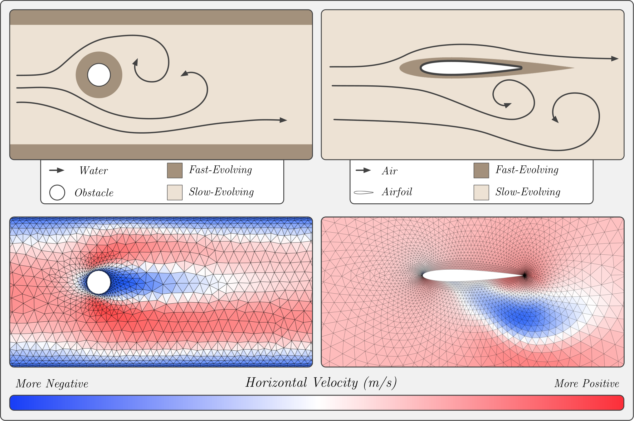
The ability to model non-uniform discretizations of the PDE domain is important for balancing the tradeoff between computational cost and solution accuracy. Classical numerical solvers rely on the assumption that the solution is sufficiently smooth between collocation points to maintain stability (Kochkov et al. 2021b). However, phenomena such as shockwaves and solid objects impeding flows, as we visualize in Figure 35, introduce local regions of steep gradient that require expensive high-resolution discretizations to maintain this smoothness (Berger and Oliger 1984). Uniform discretizations wastefully allocate the same high resolution required in these isolated regions even in areas where the dynamics are slower-evolving (Wu et al. 2022b). To address this limitation, non-uniform meshes allocate fine resolution in high-gradient regions and coarse resolution elsewhere. Furthermore, the geometry of the mesh can adapt as high-gradient regions shift in space, as is commonly the case for time-evolving PDEs (Berger and Oliger 1984).
While machine learning methods have been shown to allow for coarser discretizations than numerical methods due to their ability to learn a direct mapping (Kochkov et al. 2021b; Stachenfeld et al. 2021), neural networks still benefit from a certain level of continuity in the solution space. In addition to the inefficiency for dynamics with isolated regions of high gradient, surrogate models built on the CNN architecture cannot directly model non-rectangular domains, for example, fluid flow around a cylinder. These limitations have given rise to a number of approaches for modeling dynamics on non-uniform meshes and learned mesh adaptation.
Due to their ability to learn with unstructured data, GNNs (Kipf and Welling 2017; Gilmer et al. 2017) have been a primary choice for modeling dynamics on irregular meshes. Pfaff et al. 2021 take this approach in their MeshGraphNets framework, where they train a message-passing GNN to model a time-evolving PDE autoregressively. The input graph for MeshGraphNets is constructed with the nodes representing the PDE solution evaluated on a non-uniform mesh at the current time step, and the target nodes as the solution at a future time step. The MeshGraphNets framework additionally involves a second GNN that predicts the sizing tensor for each node. The predicted sizing tensor is then used by an adaptive mesh refinement algorithm to update the mesh geometry as dynamics evolve. However, this re-meshing algorithm is expensive and furthermore may not produce the optimal geometry in terms of the tradeoff between solution accuracy and cost of the mesh (Wu et al. 2022b). Thus, Wu et al. 2022b propose Learning controllable Adaptive simulation for Multi-resolution Physics (LAMP), a faster, data-driven approach to re-meshing using reinforcement learning. They jointly optimize the dynamics GNN and a mesh refinement policy, where the policy is selected by simultaneously minimizing the error of the dynamics GNN and the number of nodes in the mesh. Beyond standard message passing, Janny et al. 2023 utilize global attention in their dynamics GNN to model turbulent flows on a mesh, managing complexity by pooling nodes prior to attention computations.
DeepONets are a general operator learning framework beyond GNNs developed based on the Universal Approximation Theorem for Operators (Chen and Chen 1995) which have demonstrated success on a variety of operator regression tasks including learning the solution operator for PDEs (Lu et al. 2021b). The input to DeepONet is a function discretized onto an arbitrary geometry and a query point . DeepONets then aim to map to a given target function evaluated at point . In the context of a PDE, may be the boundary conditions, initial conditions, or forcing term, and is the PDE solution. The primary components in the DeepONet framework are a branch network , which encodes to , and a trunk network to encode to . While the trunk network is often chosen to be a MLP, the architecture of the branch network can be freely chosen dependent on the discretization of the input function. For example, if is discretized onto a regular grid, can be a CNN, while a GNN branch network can be used for irregular discretizations (Lu et al. 2022a). DeepONet then takes the dot product of the output vectors from the two networks to approximate the target function evaluated at the query point as . Intuitively, while the branch network learns basis coefficients conditioned on , the trunk network learns basis functions evaluated at point , and can even be replaced with a fixed basis determined by the training data, such as the Proper Orthogonal Decomposition (Bhattacharya et al. 2021) as in Lu et al. 2022a.
The DeepONet framework is flexible, with the only constraint being that the discretization of the input function be identical for all training pairs, however, several works have extended DeepONet to relieve this constraint (Kovachki et al. 2021). This mesh-independence is a defining factor for neural operators, which, as discussed in Section 9.2.3, aim to learn PDE solution operators while maintaining the ability to generalize beyond the discretization of the training data (Kovachki et al. 2021). The attention mechanism has been shown to be a special case of a neural operator layer (Kovachki et al. 2021), and thus, there have been several works developing transformer-based frameworks for modeling dynamics on irregular meshes. For tokens with a -dimensional embedding, Cao 2021 removes softmax and views the query, key, and value matrices as learned basis functions evaluated at mesh points. Attention calculations then facilitate an integration-based interpretation, bearing resemblances to a Fourier-type kernel integral transform or a Petrov-Galerkin-type projection.
Under this interpretation, Cao 2021 propose Fourier-type attention and Galerkin-type attention, the latter of which has linear complexity and is proven to possess quasi-optimal approximation capacity. However, since both Fourier and Galerkin-type attention are based on self-attention, they cannot handle the setting where the discretization of the input function differs from that of the target function , i.e., the query points . OFormer (Li et al. 2022d) therefore leverages cross-attention to adapt Galerkin-type attention to this case, with keys and values as the embedded discretization of and the queries as the embeddings. This conditions the embeddings for the query points on the input function, a formulation shown to have connections to DeepONet. Li et al. 2022d empirically demonstrate that this spatial encoding is sufficiently expressive such that given the embeddings, the PDE is reduced to an ODE in latent space. Specifically, following the embedding of , temporal evolution of the system no longer requires spatial updates and can be accomplished in latent space simply through recurrent application of a point-wise MLP to each of the embeddings.
Hao et al. 2023 build on OFormer by extending to the case where there are multiple input functions that are discretized on different grids in constructing their General Neural Operator Transformer (GNOT). GNOT furthermore replaces the point-wise MLP applied in Transformer encoder layers with a Geometric Gating Mechanism. This mechanism consists of a mixture of MLPs, where the mixture weights for a given query point are determined by a gating MLP, effectively permitting the point-wise update to vary with .
GNNs have also played a fundamental role in the development of neural operators. Li et al. 2020a demonstrate a connection between message passing in GNNs and the Green’s function formulation of the PDE solution in their Graph Kernel Network (GKN). Under this formulation, the solution of a linear PDE can be written as an integral involving a kernel function. Then, the Monte Carlo approximation to this integral produces a sum that closely resembles message passing given an assumption of locality on the integral, that is, by restricting neighbors of each mesh point to be the mesh points within a fixed radius. Because the Monte Carlo approximation includes normalization by the neighborhood size, learned message passing in GKN can generalize well to graphs with an arbitrary number of neighbors per node, an ability which becomes relevant when performing inference on a mesh with a resolution differing from that observed during training. Li et al. 2020a extend the Green’s function formulation to non-linear PDEs through the inclusion of non-linearities, and improve the efficiency of GKN through a Nyström approximation of the kernel which reduces the Monte Carlo sum over the full neighborhood to a sum over randomly sampled sub-neighborhoods.
While the locality assumption imposed on integrals by GKN ensures computational efficiency, it does not allow long-range interactions between distant mesh points and thus cannot capture global properties of the solution operator (Li et al. 2020b). Li et al. 2020b therefore propose the Multipole Graph Kernel Network (MGKN) for efficiently modeling long-range interactions. MGKN is centered on a V-cycle algorithm inspired by multi-grid methods (Han et al. 2021a) and the classical Fast Multipole Method, a method originally developed to approximate pairwise interactions for -body simulation in time using a hierarchical decomposition of space to model increasingly distant particle interactions (Cipra 2000; Greengard and Rokhlin 1987). The V-cycle algorithm operates similar to a graph U-Net (Gao and Ji 2019), processing a hierarchy of graphs representing interactions at increasingly distant scales along a downsampling and upsampling path. MGKN composes multiple V-cycles wherein latent graphs are processed using message passing, with graphs processed at each scale of the downsampling path obtained as a subgraph of the graph processed at the previous scale. Li et al. 2020b demonstrate improved performance and efficiency of MGKN relative to GKN. Additionally, since message passing on a given graph in MGKN is done identically to GKN, MGKN retains the ability to generalize to discretizations differing from those observed in training.
Li et al. 2022b instead look to model long-range interactions on irregular geometries using global Fourier convolutions similar to the Fourier Neural Operator (FNO) discussed in Section 9.2.3, a challenge since the Fast Fourier Transform is restricted to regular grids. The Geometry-aware FNO (Geo-FNO) therefore uses a geometric Fourier transform in its first and final convolution layers. The geometric transform in the first layer maps from a function on the irregularly-meshed spatial domain to a function in the frequency domain corresponding to a uniform grid using a learned mapping from mesh coordinates to uniform grid coordinates. This enables use of the computationally-efficient Fast Fourier Transform for the remaining convolutions. In the final layer, the inverse geometric transform is applied to map back to the irregularly-meshed spatial domain. This architecture was later optimized for depth alongside the conventional FNO by Tran et al. 2021 with their Factorized FNO (F-FNO).
Despite its efficiency in capturing long-range interactions on irregular geometries, use of the geometric Fourier transform by Geo-FNO prevents it from generalizing well to discretizations differing from those observed during training (Li et al. 2023c). Li et al. 2023c thus integrate the GKN and FNO architectures in the Geometry-Informed Neural Operator (GINO), which leverages a GKN encoder and decoder with an FNO processor in latent space. Specifically, a GKN module is used to obtain a latent representation on the input irregular mesh. Because the radius graph-based message passing utilized by GKN allows for arbitrary mesh points to be queried, this irregularly-meshed representation can be queried on a regular grid. The FNO processor in GKN can then process long-range interactions in this representation efficiently using the fast Fourier transform. Finally, a second GKN is applied to the output regularly-meshed representation to map back to the input geometry following an analogous approach to the encoder GKN. This framework allows GINO to generalize beyond the resolution of the training data while also enabling modeling of long-range dependencies on irregular meshes. Li et al. 2023c demonstrate the ability of GINO to accurately model turbulent dynamics on irregular geometries in 3 spatial dimensions with a large number of mesh points.
9.2.5. Existing Methods: Long-Term Stability
Time-evolving PDEs are numerically solved by discretizing the temporal domain into time steps on which the solver produces solutions. As discussed in Section 9.1, this solution can be obtained using an explicit scheme, wherein the solution at a given time point is directly calculated using the preceding solution as for some function , or implicit schemes, which entail solving a system of (possibly non-linear) equations involving and (Olver 2014). Although explicit schemes appear to require less computational effort than implicit, classical solvers that advance time using an explicit scheme can exhibit conditional stability, meaning that the discretization in time must be chosen sufficiently fine to prevent the solver from diverging (Courant et al. 1928; Olver 2014). Such PDEs for which explicit methods require significantly finer time discretizations compared to the smoothness of the actual solution are termed stiff. As a result, implicit methods have been traditionally preferred for solving stiff PDEs. Nonetheless, many neural surrogates utilize explicit schemes for convenience, and have been shown to outperform classical solvers on computationally inexpensive coarse discretizations with large time steps (Kochkov et al. 2021b; Stachenfeld et al. 2021). However, explicit schemes inevitably introduce error to the inputs of the model, and thus, increasing the robustness of neural solvers to noisy inputs is key for enabling stable predictions over many time steps.
The task often considered in this setting is to predict the rollout up to time step conditioned on the first solutions, that is, the mapping . In what follows, we take for simplicity in notation such that the mapping to be learned is from the time solution to the remaining steps, but this is not necessary in general. For such a task, explicit schemes train for a one-step prediction of conditioned on the ground-truth solution at , and at test time predict the full rollout by applying the trained network autoregressively times (Li et al. 2021c; Brandstetter et al. 2022c; Sanchez-Gonzalez et al. 2020; Stachenfeld et al. 2021; Lippe et al. 2023; Kohl et al. 2023). This one-step training strategy has been shown to be more effective than training recurrently to predict the full rollout (Tran et al. 2021). However, it is not representative of the task at test time, since for , the input to the model will not be the ground truth as in training, but rather , where is the error accumulated up to time through autoregressive prediction of . Because is often monotonically increasing with , rolling out chaotic dynamics such as turbulent flows for many time steps can be prohibitively difficult for machine learning methods to do accurately in terms of mean squared error. However, stable, long-time simulation of dynamics that exhibit accurate behavior elsewhere can hold value, for example, in terms of the Fourier spectrum (Li et al. 2021c; Lippe et al. 2023; Kohl et al. 2023), principal components (Li et al. 2021c), Pearson correlation (Lippe et al. 2023), rate of change (Kohl et al. 2023), and other summary statistics which characterize the behavior of the system over long time horizons.
Li et al. 2021c study chaotic dynamics with the physical property of dissipativity, which ensures that regardless of their initial conditions, given sufficient evolution, the dynamics will eventually arrive and remain in a particular set of states referred to as the absorbing set, allowing reproducible statistics to be computed even for trajectories with diverse starting points. Li et al. 2021c therefore look to induce dissipativity in training their Markov Neural Operator (MNO), enabling accurate computation of statistics from predicted rollouts. MNO is an autoregressive instantiation of FNO with soft and hard dissipativity constraints. During training, the soft constraint is applied in the form of a dissipativity-inducing loss, whereas the hard constraint is an unlearned post-processing step which forces the predicted trajectory back into a pre-determined stable region should MNO predict a transition outside of this region. MNO is also trained using a Sobolev loss, which is suggested to more reliably capture high-frequency details in the dynamics.
Other works have also taken regularization-based approaches to enhancing long-term stability, including the Lyapunov regularizer (Zheng et al. 2022) and adversarial noise injection (Sanchez-Gonzalez et al. 2020; Brandstetter et al. 2022c). Noise injection approaches intentionally corrupt inputs during training with an approximation to the prediction error . Sanchez-Gonzalez et al. 2020 apply this strategy in training their Graph Network-based Simulator (GNS) by assuming that follows a 0-mean Gaussian distribution with variance chosen as a hyperparameter. Although this approach is convenient since the noise distribution can be easily sampled, the normality assumption may not be valid, and furthermore, the variance hyperparameter controlling the noise level must be carefully tuned. Brandstetter et al. 2022c instead obtain the noise to train their Message Passing PDE solver (MP-PDE) directly from the model to reduce the distributional shift between the training noise and the test noise. They accomplish this by letting such that the input to the model is . Thus, the noise added to the inputs during training is directly sourced from the model, as it will be during testing.
Lippe et al. 2023 maintain the normality assumption in in their PDE-Refiner framework and propose to choose several noise levels based on the amplitudes in the Fourier spectra of the PDE solution. This sequential noise injection strategy is motivated by analysis showing that standard MSE-loss with 1-step training objectives neglects frequency components with smaller amplitudes, and that errors on these components accumulate over many time steps, permeating into higher-amplitude components where errors are more noticeable. To improve the 1-step prediction of smaller amplitudes, Lippe et al. 2023 apply their neural solver multiple times to advance the rollout by 1 time step, with each forward pass following the first one serving to iteratively refine the solver’s initial prediction on increasingly smaller amplitudes. Since smaller noise levels correspond to smaller amplitudes, Lippe et al. 2023 achieve this by injecting noise at increasingly smaller levels to the model’s predictions at each refinement step during both training and inference, where, similar to denoising diffusion models (Ho et al. 2020), the prediction target for refinement steps is the injected noise which is subsequently subtracted away from the predicted solution during inference. On several time-evolving fluid dynamics tasks, PDE-Refiner demonstrates not only substantial increases in rollout stability using only 3 refinement steps, but also improved sample complexity and the ability to detect instability in predictions.
Kohl et al. 2023 also employ diffusion models in the setting of time-evolving fluid dynamics for enhanced rollout stability. However, instead of a refinement-based approach, Kohl et al. 2023 frame 1-step prediction as a conditional generation task, where their Autoregressive Conditional Diffusion Model (ACDM) is tasked with denoising both the state at the next time step as well as the previously predicted states with noise added. By learning to denoise the conditioning states, Kohl et al. 2023 aim to increase the robustness of ACDM to errors introduced in prediction of the previous states. Kohl et al. 2023 show that ACDM can preserve the correct statistics for the flow over longer rollouts in a variety of fluid simulation settings. Additionally, the ability of ACDM to produce diverse yet physically-consistent samples from the posterior distribution of PDE solutions is demonstrated, an ability relevant for uncertainty quantification.
While Tran et al. 2021 found training for recurrent prediction of full rollouts to be suboptimal compared to 1-step prediction, several works have trained models to recurrently predict only a few steps ahead (Wu et al. 2022d; Lam et al. 2022). Wu et al. 2022d implement this strategy in optimizing their Hybrid Graph Network Simulator (HGNS) using a multi-step objective. The total loss is a weighted sum of the loss at each time step, with the one-step loss weighted heaviest so that the optimization initially targets short-term predictions before fine-tuning for longer-term predictions. This method is more stable than full recurrent prediction since it only predicts several steps ahead, and not the full rollout.
Several works have successfully adopted fully-recurrent prediction in latent space through the use of autoencoders (Han et al. 2021a; Wu et al. 2022a). Han et al. 2021a specifically consider rolling out irregularly-meshed dynamics for many time steps with their Graph Mesh Reducer Transformer (GMR-Transformer). In this framework, a GNN encoder and decoder are trained in an autoencoding fashion to map the system at a given timestep to and from a latent vector, respectively. This reduced latent representation is memory-efficient and therefore allows Han et al. 2021a to recurrently train a Transformer to predict the latent vectors for each state of the rollout, which can subsequently be upsampled from the latent space using the GNN decoder. GMR-Transformer demonstrates the ability to accurately predict rollouts of fluid dynamics in irregularly-meshed domains for hundreds of time steps.
While the previously discussed architectures predict only one step ahead, Brandstetter et al. 2022c make the observation that since each forward propagation introduces some error, reducing the number of calls to the model required to predict a rollout could reduce the total accumulated error. Instead of predicting only one time step ahead as , Brandstetter et al. 2022c train their model to predict steps ahead with one forward propagation as . For example, to predict timesteps with , only 5 forward propagations are required instead of 10. Following a similar philosophy, Bi et al. 2022 introduce hierarchical temporal aggregation for their learned weather forecasting model, wherein several models are trained with different time step sizes. At inference time, the rollout is divided between the models such that the minimal number of forward passes are required to advance the system forward to the target lead time.
9.2.6. Existing Methods: Preserving Symmetries
Dynamic systems are governed by the laws of physics, with symmetries of systems related to these laws through Noether’s theorem (Noether 1971; Wang et al. 2021c). The symmetry group of a PDE characterizes the transformations under which solutions remain solutions, e.g., for a PDE with rotation symmetry, rotating the solution function produces a function that is also a solution. Symmetries such as rotation invariance are understood intuitively as the lack of canonical reference frame that allows, for example, a 2-dimensional flow rotated by to remain equally physically plausible. Other symmetries such as translation invariance arise in PDEs with infinite domains or periodic boundaries (Holmes et al. 2012). Priors that enforce symmetries can improve generalization and sample complexity by reducing the size of the model search space (Raissi et al. 2019; Wang et al. 2021c; Brandstetter et al. 2022b). Furthermore, PDEs with spherical domains commonly arising in global weather forecasting applications (Esteves et al. 2023; Bonev et al. 2023) have led to the application of tailored architectures to ensure that symmetries are preserved.
As a method of instilling learned equivariance, Brandstetter et al. 2022b propose Lie Point Symmetry Data Augmentation (LPSDA) to improve sample complexity and the generalization ability of neural solvers by leveraging symmetries of the PDE. Similarly, Akhound-Sadegh et al. 2023 introduce a symmetry loss in training the Physics-Informed DeepONet proposed by Wang et al. 2021d, allowing the network to learn a family of PDE solutions related by a symmetry transformation by learning only one member.
Equivariant CNNs, which are composed of convolutional layers that automatically encode the desired symmetry (Cohen and Welling 2016; Cohen and Welling 2017; Weiler et al. 2018; Weiler and Cesa 2019; Worrall and Welling 2019; Weiler et al. 2023), present an alternative path to achieving equivariance. Wang et al. 2021c consider a variety of symmetries in constructing their Equ-ResNet and Equ-Unet for dynamics forecasting, including exact scale and rotation symmetries. However, dynamics often only exhibit approximate symmetries due to, for example, external forces (Wang et al. 2022i). Wang et al. 2022i thus relax equivariance constraints in 2 spatial dimensions in constructing their RGroup and RSteer CNNs for approximately equivariant group and steerable convolutions, respectively (Cohen and Welling 2016; Cohen and Welling 2017). Wang et al. 2022i learn their convolution kernels as a linear combination of equivariant kernels , where the weight corresponding to the -th kernel in the linear combination is learned and is itself a function on the group as opposed to a scalar value. In doing so, exact equivariance is recovered when the are identical for all . Wang et al. 2023c demonstrated that the learned adapt as expected when the symmetry of the mapping to be learned is equal to, less than, or completely absent relative to the symmetry encoded by the network. Wang et al. 2023c furthermore extended approximately rotation-equivariant group convolutions to 3 spatial dimensions with the R-Equiv architecture following a similar approach as in 2 spatial dimensions. However, the number of parameters increases in each kernel since the number of possible rotations increases from 2 dimensions to 3. Therefore, to improve parameter efficiency, Wang et al. 2023c apply a rank-1 tensor decomposition to their relaxed kernels, as is done in separable group convolutions (Knigge et al. 2022). In experiments on turbulent flows with a range of symmetry levels, Wang et al. 2023c highlight the advantages of their approach and furthermore offer interpretability in the weights as to how dynamics break symmetries. Beyond equivariant convolutions, Holderrieth et al. 2021 equivariantly model stochastic fields by extending steerability constraints to Gaussian Processes and Conditional Neural Processes.
Instead of steerable or group convolutions, Ruhe et al. 2023a encode symmetries using Clifford algebras. Multivectors, the elements of Clifford algebras, have scalar components, vector components, and higher-order components representing plane and volume segments, with multivector multiplication defined with the geometric product (Brandstetter et al. 2023). Brandstetter et al. 2023 note that the standard practice of stacking vector and scalar fields comprising PDE solutions along the channel dimension in neural solvers does not model the geometric relationships between fields well. Instead, Brandstetter et al. 2023 represent these fields as multivectors, resulting in multivector feature maps and kernels that are convolved with Clifford CNN layers and Clifford FNO layers operating via the geometric product in the CResNet and CFNO architectures, respectively.
As dynamics tasks often involve a target which is a geometric transformation of the input, Ruhe et al. 2023b build on Brandstetter et al. 2023 by learning compositions of transformations with their Geometric Clifford Algebra Network (GCAN). The construction of the GCAN is based on the result that transformations of an arbitrary multivector by (i.e., rotations, reflections, and translations) can be achieved through geometric products of with other multivectors chosen dependent on . Group action layers in the GCAN therefore apply learned transformations to the input multivector through geometric products with learned multivectors, where the range of possible transformations is determined by the choice of the basis for the algebra, ranging from to . Through appropriate selection of multivector representation for various data types, Ruhe et al. 2023b demonstrate the flexibility of the GCAN, allowing for simulation of rigid body transformations with GCA-MLP and GCA-GNN, as well as simulation of fluid dynamics with GCA-CNN.
Ruhe et al. 2023a extend this work by using Clifford algebras in the derivation of their -equivariant Clifford Group Equivariant Neural Network (CGENN). Unlike previous equivariant architectures, CGENNs achieve equivariance through symmetry properties of several multivector operations. Specifically, Ruhe et al. 2023a prove the -equivariance of the geometric product, multivector grade projections, wherein all the multivector components excluding the -th order part are set to 0, and polynomial functions of multivectors. Equivariant linear layers in the CGENN architecture then learn coefficients used to linearly combine grade projections of multivectors comprising the channels of neural representations. Additionally, Geometric Product Layers consider pair-wise interactions between channels by learning to linearly combine compositions of various grade projections with geometric products applied to channels. Ruhe et al. 2023a demonstrate performance gains with the CGENN architecture on a variety of diverse tasks wherein symmetries play a role, including -body simulation in 3 spatial dimensions.
While the previously discussed equivariant CNNs perform convolution in physical space, Helwig et al. 2023 extend group equivariant convolutions (Cohen and Welling 2016) to a frequency domain parameterization with the -FNO architecture. -equivariant convolutions convolve kernels and feature maps that are functions on the group , whereas the discrete Fourier transform is only defined for functions on the grid , thereby complicating the use of the Convolution Theorem which enables Fourier-space convolutions in FNOs. However, the groups considered by Helwig et al. 2023 are the semi-direct product of the plane with a subgroup , where is either rotations for or roto-reflections for . Using this decomposition, group convolutions can be expressed as a sum of planar convolutions with a kernel transformed by an element of . Applying the Convolution Theorem to these planar convolutions gives point-wise multiplication with the Fourier transform of the kernel transformed by an element of , . Finally, Helwig et al. 2023 apply symmetries of the Fourier transform which allow orthogonal transformations, including elements of , to commute with the Fourier transform, giving and enabling equivariant convolutions parameterized in the frequency domain. In addition to the benefits brought in terms of multi-scale processing as discussed in Section 9.2.3, this allows for superior generalization to discretizations with different resolution relative to physically parameterized alternatives (Li et al. 2021b).
Similar to FNOs, spherical CNNs (Cohen et al. 2018; Kondor et al. 2018; Esteves et al. 2020) learn the generalized Fourier transform of convolution kernels to address challenges associated with convolving spherical signals in a rotation-equivariant manner. Spherical data arises in the context of PDEs for global climate and weather forecasting tasks, where the fields to be modeled, such as wind velocity or air pressure, are defined on the globe. However, application of conventional CNNs to such spherical data requires that it be projected into the plane, resulting in distorations (Cohen et al. 2018). The vision transformer-based weather forecasting methods discussed in Section 9.2.3 encounter the same distortion due to their reliance on splitting the input spherical fields into sequences of equal-sized, square patches (Dosovitskiy et al. 2021). Furthermore, it is difficult to correctly model boundary conditions after projecting from the sphere to the plane, as boundary points which appear spatially distant following the projection may be immediately adjacent in reality.
To address these challenges, Bonev et al. 2023 introduce the spherical FNO (SFNO), a spherical CNN for modeling global weather, and demonstrate the strengths of their architecture in stably generating year-long forecasts more than 1,000 time steps in length. Esteves et al. 2023 similarly employ spin-weighted spherical CNNs (SWSCNNs) (Esteves et al. 2020) for global forecasting, and introduce several enhancements including an optimized calculation of the generalized Fourier transform, spectral batch norm, spectral pooling, and spectral residual connections which enable training of spherical CNNs at scale. Additionally, SWSCNNs equivariantly model vector fields on the sphere (Esteves et al. 2020), a challenge beyond scalar fields since the rotation of individual vectors must be considered in addition to rotation of the field. This ability could enhance modeling of physical quantities such as the vector-valued velocity field for global winds.
Horie et al. 2021 further consider modeling dynamics on irregular geometries with their IsoGCN architecture, an -equivariant GNN which simplifies Tensor Field Networks (Thomas et al. 2018) for improved space-time complexity by not relying on spherical harmonics and by building on the linear message passing scheme used in Graph Convolutional Networks (Kipf and Welling 2017). IsoGCN leverages the IsoAM, an -equivariant adjacency matrix representation containing spatial information. In addition to equivariance, Horie et al. 2021 demonstrate physical motivation in their construction of the IsoAM by proving that convolution, contraction, and tensor product operators applied to IsoAM and the tensor field of node features can yield various differential operators applied to the tensor field, including the gradient, divergence, and Jacobian operators. As a result of the improved computational efficiency in IsoGCN, Horie et al. 2021 demonstrate the ability to simulate the evolution of a heat field on CAD objects in three spatial dimensions on a mesh with more than 1 million collocation points. Toshev et al. 2023 similarly consider three spatial dimensions, but instead utilize the -equivariant SEGNN architecture (Brandstetter et al. 2022a) to simulate a flow of fluid particles under a Lagrangian scheme.
9.2.7. Existing Methods: Incorporating Physics
While deep neural networks are universal function approximators, practitioners often have insight into the behavior of physical systems. By carefully designing architectures to automatically respect physical laws that these systems obey, the learning task is simplified and the ability of the network to generalize over similar systems is improved. This is because these rules are difficult to learn from data directly, particularly in the small data regime. Further, encoding physical laws often increases the interpretability of network outputs, as they can be directly related to concepts practitioners are familiar with, which is in stark contrast to the usual treatment of neural networks as a black box modeling tools.
Hamiltonian Neural Networks (HNNs) (Greydanus et al. 2019) incorporate physics knowledge in the form of Hamiltonian mechanics for faithful modeling of Hamiltonian systems. In general, these systems are described by position and canonical momenta , which evolve in time according to Hamilton’s equations as
| (114) |
where and are the derivatives of and with respect to time. Hamiltonian systems are everywhere – the motion of planets under the influence of gravity, particles impacted by electromagnetic forces, and blocks attached to springs all follow Hamiltonian mechanics. A key property of Hamiltonian systems is that as the system state denoted by evolves over time, the Hamiltonian is conserved, that is, it remains constant. Loosely, the Hamiltonian captures the amount of energy in the system. HNNs (Greydanus et al. 2019) propose learning this Hamiltonian directly from dynamics data. Instead of directly supervising their model such that , Greydanus et al. 2019 apply supervision on the gradients of the network to satisfy Equation 114 as
| (115) |
where, similar to the approach taken by Physics Informed Neural Networks discussed later, the partial derivatives of in Equation 115 are computed exactly using automatic differentiation. The time evolution of the Hamiltonian system is then computed by numerically integrating Equation 114 with in place of over time using an explicit Runge-Kutta method of order . The HNN model accurately learns the time evolution of simple Hamiltonian systems such as an oscillating pendulum without dissipating energy, making predictions that maintain consistency with Hamilton’s equations. In contrast, a standard fully-connected neural network trained on the same data is unable to learn trajectories that conserve , resulting in physically implausible predictions.
Sanchez-Gonzalez et al. 2019 extend HNNs to the Neural ODE framework (Chen et al. 2019a) with their Hamiltonian ODE graph network (HOGN) by backpropagating through the numerical integrator such that the optimization of takes the form of
| (116) |
where the numerical integrator approximates the integration given by
| (117) |
Unlike Equation 115, Equation 116 does not impose explicit supervision on the temporal derivatives of , and instead learns these quantities implicitly by backpropagating through the numerical integrator. As this implicit approach instead only requires the system state instead of the temporal derivatives for model training, a number of works have extended it beyond Hamiltonian systems. These works commonly perform numerical integration using the forward Euler method given in Equation 109, as it is one of the most straightforward implementations of Equation 117. Sanchez-Gonzalez et al. 2020; Pfaff et al. 2021; Toshev et al. 2024a; Toshev et al. 2024b train models to predict per-particle acceleration in Lagrangian simulations which are integrated twice to update particle positions. For Eulerian simulations, many works predict the residual between and (Pfaff et al. 2021; Stachenfeld et al. 2021; Lippe et al. 2023; Price et al. 2023), where the update can be interpreted as integration with the forward Euler method.
In theory, the current state of a Hamiltonian system completely determines its state at all future times . With this motivation, SympNets (Jin et al. 2020) directly learn the mapping from the current system state to the future system state using symplectic normalizing flows to avoid integrating over time. This makes SympNets more efficient over longer rollouts, as they avoid accumulation of numerical errors present during numerical integration. Symplectic Recurrent Neural Networks (Chen et al. 2020b) further improve upon Hamiltonian Neural Networks by using symplectic integrators such as the leapfrog method, which are a better fit for Hamiltonian systems than explicit Runge-Kutta schemes because they explicitly match the form of Equation 114. Thus, the symplectic integrator will conserve the learned Hamiltonian when integrating over time up to numerical precision. Further, Chen et al. 2020b propose training over longer rollouts produced by sampling the model recurrently instead of single-step predictions. This helps avoid the distributional shift problem inherent when recursively sampling from the model’s predictions at each time step, as discussed in Section 9.2.5. Finally, to account for noise in the system observables, Chen et al. 2020b update the initial state via gradient descent. These modifications improve the accuracy of the HNN when modeling noisy, real-world systems.
Instead of general Hamiltonian systems, Action-Angle Networks (Daigavane et al. 2022) leverage properties of the special class of integrable Hamiltonian systems by learning a symplectic transformation of position and momenta to slow-varying action variables and fast-varying angle variables. For integrable systems, the dynamics in the action-angle space are effectively linear, which makes it both easier to learn and more efficient to numerically integrate compared to HNNs and Neural ODEs (Chen et al. 2019a).
As opposed to Hamiltonian systems, Lagrangian Neural Networks (LNN) (Cranmer et al. 2020) model Lagrangian systems where the form of the canonical momenta is not necessarily known. Instead, Lagrangian mechanics provide the necessary insight to relate the time evolution of the position as
| (118) |
where and are the first and second derivatives of the position with respect to time, and is the Lagrangian of the system. Analogous to HNNs with the Hamiltonian , LNNs model the Lagrangian via a neural network. Then, by numerically integrating Equation 118, the time evolution of can be obtained.
Finally, Sosanya and Greydanus 2022 augment HNNs to additionally predict a Rayleigh dissipation function together with the Hamiltonian . This allows the network to capture external forces such as friction which dissipate energy. Such forces cannot be captured in the original HNN framework because the HNN learns energy-conserving dynamics. The Dissipative HNN shows improved performance on predicting the time evolution of damped spring-block systems and the velocity fields of ocean surface currents.
While Hamiltonian mechanics can describe a large number of physical systems, in many real world scenarios, the system may not be sufficiently well understood or only partially observed. If the underlying PDEs describing the system are only partially known, physical knowledge can be leveraged in a hybrid setup. In this context, deep neural networks can be applied in conjunction with PDE-based methods to learn the residual between assumed governing equations and observed data. A representative example is the APHYNITY framework proposed by Yin et al. 2021, which operates on the premise that dynamics can be decomposed into physical (known) and augmented (residual) components as
| (119) |
where represents the data-driven component that complements the known operator . When learning the parameters of , numerical integration is used to generate predictions at various steps based on given an initial state. More importantly, it efficiently augments physical models with deep data-driven networks in such a way that the data-driven model only models what cannot be captured by the physical model. To achieve this, other than prediction loss, an additional L2 norm term is imposed on . This avoids the situation that all or most of the dynamics could be captured by neural nets and the physics-based models contribute little to learning.
Similarly, DeepGLEAM (Wu et al. 2021) is a method used for predicting COVID-19 mortality by directly combining the mechanistic epidemic simulation model GLEAM with neural nets. GLEAM (Balcan et al. 2009) is a PDE-based model that characterizes complex epidemic dynamics based on meta-population age-structured compartmental models. DeepGLEAM employs a DCRNN (Li et al. 2017b) to learn the errors made by GLEAM, resulting in enhanced performance for one-week ahead COVID-19 death counts predictions.
Beyond applications to observed dynamics data, hybrid methods can be used to substitute the computationally intensive components of classical solvers or learn corrections for classical solvers applied on inexpensive but error-inducing coarse discretizations. Belbute-Peres et al. 2020 introduce a novel approach termed CFD-GCN that combines graph convolutional neural networks with a Computational Fluid Dynamics (CFD) simulator. This hybrid method aims to generate accurate predictions of high-resolution fluid flow. It runs a fast CFD simulator on a coarse triangular mesh to generate a lower-fidelity simulation, which is subsequently enhanced by upsampling it to finer meshes using the K-nearest neighbor interpolation technique. The fine-grained simulation is then processed by a graph convolutional neural network, which further refines the predictions for specific physical properties. Similarly, Kochkov et al. 2021b utilize CNNs to perform learned interpolation and learned correction on coarse velocity components produced by classic numerical solvers, leading to significant speedup in simulating high-resolution fluid velocity fields. Moreover, Tompson et al. 2017 replace the numerical solver for solving Poisson’s equations, which is the most computationally expensive step in the procedure of traditional Eulerian fluid simulation, with a convolutional network. This approach results in significant speedup and demonstrates physically consistent predictions with strong generalization abilities.
As opposed to approximating the numerical PDE solution as in the previously discussed works, Physics-Informed Neural Networks (PINNs) aim to approximate the analytical solution by parameterizing the neural network as the PDE solution (Raissi et al. 2019). Using backpropagation, the spatial and temporal derivatives in Section 9.1 can be exactly evaluated and used as a regularizing agent in an effort to ensure that the constraints prescribed by Section 9.1 are approximately satisfied. Thus, for the operator defined as
| (120) |
the network can be optimized over the parameter space as
| (121) |
, , and are coefficients for balancing different loss terms, which require careful tuning. PINNs have found real-world applications in biomedical analyses of blood flow (Raissi et al. 2020) with the Hidden Fluid Mechanics framework, and have been coupled with data-driven neural solvers such as the Physics-Informed DeepONet (Wang et al. 2021d) and Physics-Informed Neural Operator (Li et al. 2021g) to improve sample complexity and even allow for fully self-supervised training. Yang et al. 2021b further propose B-PINNs, which extends the concept of PINNs into the Bayesian framework. Under this approach, a PINN is used as the prior for solving partial differential equations (PDEs), while the Hamiltonian Monte Carlo method is employed to draw samples from the resulting posterior distribution. Compared with PINNs, B-PINNs not only provide uncertainty quantification but also obtain more accurate predictions on noisy data due to their ability to avoid overfitting.
PINNs draw several key contrasts to the operator-learning approach detailed in Sections 9.2.3 and 9.2.4. The operator learning paradigm trains to inductively map functions in the input space to the target function space. While this enables generalization over PDE configurations , such as initial conditions or PDE parameters, training requires discretization of the functions. In contrast, if is a PINN, training can be mesh-free, as takes the form of a function approximating the analytical solution to the PDE. However, this ties the trained model to one particular realization of , as the solution of a PDE with configuration is not likely to also be the solution with configuration , thereby requiring re-training of for each new instance of the PDE. To mitigate re-training cost, Cho et al. 2024 consider a meta-learning framework which includes a hypernetwork for parameterizing their low-rank PINN (LR-PINN) dependent on the PDE parameters . Specifically, LR-PINN is trained on a variety of realizations of a given PDE with varying PDE parameters . For the PDE parameterized by , the weight matrices that form the linear layers of LR-PINN are decomposed using the singular value decomposition as , where the and matrices are shared across all examples, while the singular values are output from a hypernetwork whose input is . Following training, given a new instance of the PDE parameterized by , only the singular values of the weight matrices are tuned starting from the hypernetwork-initialized . This greatly accelerates fine-tuning, as all remaining weights are frozen, and furthermore, the singular values from the hypernetwork are likely to be near-optimal.
9.2.8. Datasets and Benchmarks
| Dataset | Source | Fields Modeled | Spatial Dimensions | Task Details |
| Compressible Navier-Stokes | Takamoto et al. 2022a | Density, Pressure, Velocity | 1,2,3 | Initial Mach number=1 and viscosity= yield fast-moving and turbulent dynamics. |
| Shallow Water | Gupta and Brandstetter 2023 | Density, Velocity, Vorticity | 2 | Global weather on a rectangular domain with 48 hour time step. |
| Incompressible Navier-Stokes | Gupta and Brandstetter 2023 | Pressure, Velocity, Vorticity | 2 | Includes conditional task: advance the state of the system conditioned on variable timestep size and forcing term. |
| TorusVis and TorusVisForce | Tran et al. 2021 | Vorticity | 2 | Variable viscosity coefficient and forcing term. Includes time-varying forcing term. |
| CylinderFlow and AirFoil | Pfaff et al. 2021 | Momentum, Pressure, Density | 2 | Flow about obstacle on irregular mesh. |
| DeformingPlate and FlagDynamic | Pfaff et al. 2021 | Position, von-Mises Stress | 3 | Lagrangian simulation of structural mechanics. |
| Water, Sand, Goop, MultiMaterial, WaterRamps, SandRamps, FluidShake, and Continuous | Sanchez-Gonzalez et al. 2020 | Position | 2,3 | Lagrangian simulation of various materials interacting with ramps, external forcing, and variable friction. |
| Decaying Taylor-Green Vortex, Reverse Poiseuille flow, Lid-driven cavity, and Dam break | Toshev et al. 2024b | Position | 2,3 | Lagrangian simulation of fluid dynamics interacting with turbulence, external forcing, moving boundaries, and dam breakage. |
| Elasticity | Li et al. 2022b | Stress | 2 | Incompressible Rivlin-Saunders material deformed about irregularly-shaped void. |
| Plasticity | Li et al. 2022b | Deformation | 2 | Deformation due to impact with irregularly-shaped die. |
| Pipe | Li et al. 2022b | Horizontal Velocity | 2 | Incompressible flow through a curved pipe on irregular mesh. |
| Airfoil | Li et al. 2022b | Mach number | 2 | Transonic steady-state flow about an airfoil on irregular mesh. |
| AirFRANS | Bonnet et al. 2022 | Velocity, Pressure, Kinematic Viscosity | 2 | Reynolds-averaged steady-state flow about an airfoil on irregular mesh with variable angle-of-attack and Reynolds number. |
The rise of neural PDE solvers has elicited many datasets for forward PDE modeling, several of which we highlight here and summarize in Table 33. Takamoto et al. 2022a release PDEBench, which contains numerical solution data for 8 different PDEs with varying spatial dimensions. Beyond forward problems, Takamoto et al. 2022a also consider inverse problems, a task we discuss in Section 9.3. Perhaps the most challenging PDEBench dataset is the compressible Navier-Stokes equations for modeling the density, pressure, and velocity fields of a compressible fluid, which Takamoto et al. 2022a include in one, two and three spatial dimensions. Fluids with velocities approaching (subsonic) or exceeding (supersonic) the speed of sound must be considered compressible, that is, as having a density which varies due to pressure (Vreugdenhil 1994; Anderson 2017). Thus, Takamoto et al. 2022a release versions of this data with the initial Mach number, quantifying the ratio between the velocity of the fluid to the speed of sound in the fluid (Anderson 2017), as high as 1. Further, the low viscosities considered by Takamoto et al. 2022a produce highly turbulent dynamics which must be resolved at small scales for stable simulation (Kochkov et al. 2021b).
Gupta and Brandstetter 2023 consider a particularly difficult realization of the shallow water equations generated using the global atmospheric model developed by Klöwer et al. 2022. This PDE is derived by depth-integrating the Navier-Stokes equations, and, despite the name, can model fluids beyond water (Vreugdenhil 1994). This dataset of over trajectories models global pressure, wind velocity, and wind vorticity fields. Gupta and Brandstetter 2023 consider the task of advancing the system by 48 hour intervals, a coarse mapping that is especially challenging to learn. Gupta and Brandstetter 2023 also release data for modeling the incompressible Navier-Stokes equations generated by the solver (Holl et al. 2020), and consider an interesting conditional task in which the learned solver makes predictions to future timesteps conditioned on varying timestep sizes and forcing terms. Similarly, Tran et al. 2021 provide data for modeling the vorticity field of a fluid with the incompressible Navier-Stokes equations while generalizing over the viscosity coefficients and forcing terms.
The previous datasets emphasize Eulerian systems that are spatially discretized onto square, uniformly-spaced meshes, and therefore are largely dominated by convolutional models. However, as discussed in Section 9.2.4, architectures that can model dynamics on irregular geometries can balance the tradeoff between solution accuracy and computational cost, and furthermore enable modeling of a more general class of problems. Pfaff et al. 2021 demonstrate this flexibility in their dataset modeling flow around a cylinder governed by the incompressible Navier-Stokes equations, as well as a flow around an airfoil governed by the compressible Navier-Stokes equations, both of which are visualized in Figure 35. Pfaff et al. 2021 extend beyond Eulerian fluid dynamics problems with the release of structural mechanics problems modeling a flag blowing in the wind and a deformable metal plate. Importantly, these structural mechanics settings are modeled in the Lagrangian paradigm which, as discussed in Section 9.1, differs from Eulerian schemes by discretizing particles instead of space.
Multiple works have released data with an exclusive focus on Lagrangian simulations. Sanchez-Gonzalez et al. 2020 consider several datasets comprising Lagrangian simulations of a variety of materials in diverse settings. The materials modeled are water, a viscous material referred to as goop, sand, and mixtures of these materials, while the considered settings include two and three spatial dimensions, as well as ramp obstacles, external forcing in the form of a shaking container, and variable friction. The LagrangeBench datasets from Toshev et al. 2024b introduce a diverse array of Lagrangian fluid simulation datasets. While the decaying Taylor-Green vortex datasets simulate the onset of turbulence, Toshev et al. 2024b introduce a spatially-dependent external force with the reverse Poiseuille flow datasets. Additionally, the lid-driven cavity datasets impose both static and dynamic boundaries, whereas the dam-break dataset models dynamics of a fluid suddenly released from a container. Besides the dam-break setting, all LagrangeBench datasets are available in two and three spatial dimensions.
Similar to Pfaff et al. 2021, Li et al. 2022b also consider irregular geometries arising in the context of both structural mechanics and fluid dynamics simulations. In the structural mechanics setting, Li et al. 2022b release data for modeling stress of an incompressible Rivlin-Saunders material deformed about a void with a randomly-sampled, non-square geometry. Li et al. 2022b additionally release data for modeling the time-dependent deformation of a plastic material following impact with an irregularly-shaped die given the geometry of the die. Li et al. 2022b go on to study fluid dynamics problems modeling the velocity of incompressible Navier-Stokes flow though a curved pipe constructed from third-degree polynomials. Finally, Li et al. 2022b release data for modeling the Mach number of a transonic flow over an airfoil governed by the Euler equation, where transonic refers to the property of the flow as having regions moving at both subsonic and supersonic speeds. Bonnet et al. 2022 model a flow around an airfoil instead governed by the incompressible Reynolds-Averaged Navier-Stokes equations. To maintain the assumption of incompressibility, Bonnet et al. 2022 reduce the Mach number to less than 0.3, increasing difficulty by varying the angle and Mach number of the flow around the airfoil. Unlike the time-dependent fluid dynamics datasets from Pfaff et al. 2021, both Li et al. 2022b and Bonnet et al. 2022 consider steady-state fluids modeling in which the solution is static as a function of time.
We note that while these works have curated an impressive selection of challenging PDEs foundational to the study of neural solvers, solvers performing well on these tasks may not immediately generalize well to real-world applications of PDE modeling. Dynamics encountered in real-world settings can involve an interplay with complex external forces and occur in large, irregularly-shaped domains. In such settings, the previously discussed challenges of multi-scale processing (Section 9.2.3), multi-resolution modeling (Section 9.2.4), and rollout stability (Section 9.2.5) increase both in difficulty and importance. Future benchmarks should design tasks to explicitly probe these areas in more realistic scenarios.
9.2.9. Open Research Directions
We close this section on forward modeling with a discussion of challenges faced by neural solvers that have largely been unaddressed by current works.
A primary limitation of learned solvers is the requirement of an adequate number of training data generated by costly numerical solvers (Raissi et al. 2019; Brandstetter et al. 2022b), which is particularly problematic at the industry scale. Thus, improving the ability to generalize and sample complexity of learned solvers is necessary to justify and reduce this cost for their adaptation to real-world settings. Toward this goal, a richer subfield in the learned solver literature targeting techniques for out-of-distribution (OOD) dynamics should develop. In contrast to many current works that train solvers to generalize over initial conditions or PDE parameters from the same distribution as the training set, the goal of this work should be to enable learned solvers to accurately infer dynamics beyond those observed during training. Models excelling in this OOD setting will permit the span of the PDE solutions in the training set to be a subspace of the span of those in the test set, thereby improving sample complexity. OOD settings have been examined in the literature, such as Kochkov et al. 2021b, who study the performance of their hybrid classical-neural solver under OOD domain size, external forcing, and PDE parameters. Stachenfeld et al. 2021 similarly study OOD domain size, as well as OOD initial conditions and rollout length. However, there is a gap in the literature around works developing principled approaches in the regime of OOD dynamics. Initial works in this area have treated the parameters of the differential equation as environments in the context of meta-learning and trained a model that can be transductively fine-tuned at test time to adapt to unseen, OOD environments (Wang et al. 2022j; Mouli et al. 2023; Kirchmeyer et al. 2022). Similarly, as discussed in Section 9.2.3, fine-tuning physics foundation models has been shown to enable data-efficient learning of downstream dynamics modeling tasks (Subramanian et al. 2024; Hao et al. 2024; McCabe et al. 2023; Herde et al. 2024). During the pre-training stage, the model can learn the elements of simulation that are shared across diverse physics. In contrast to models trained from scratch, this learned structure has been shown to offer an initialization enabling data-efficient learning of dynamics that are OOD from the pre-training dataset.
A second factor limiting applicability is that much of the literature focuses on problems with only one or two spatial dimensions despite the prevalence of three-dimensional problems in real-world applications of PDE modeling. While many architectures discussed in this section admit an immediate extension to three spatial dimensions, in practice, three-dimensional modeling presents obstacles in the form of limited memory that must be carefully handled (Wu et al. 2022d; Lam et al. 2022; Bi et al. 2022). Beyond memory requirements, the optimization of a three-dimensional model is naturally more challenging than its two-dimensional counterpart due to the increased size of the search space. Furthermore, in three dimensions, challenging dynamics not present in lower dimensions may be introduced, such as the prominent case of turbulent flows, where the transition to three dimensions induces chaos to a degree that is unseen in two-dimensional flows due to the energy cascade discussed in Section 9.2.3 (Lienen et al. 2023). Thus, future works should look to design neural solvers that are both scalable to three spatial dimensions and that have sufficient inductive biases for the optimization to effectively navigate the search space while maintaining sufficient expressiveness to faithfully model more challenging dynamics.
Additionally, as neural networks struggle to model non-smooth functions, modeling systems with sudden changes, such as the trajectory of a ball bouncing off a wall, remains a challenge. Such problems represent an extreme version of stiffness, because the timescale of such drastic interactions is orders of magnitude smaller than the usual time step size for advancing the system. Chen et al. 2020b propose a method to handle one-time interactions of such a kind by augmenting the update equation in their integrator with a rebound module. Kim et al. 2021 propose efficient methods for computing the gradients and appropriate normalization of Neural ODEs (Chen et al. 2019a) to model stiff systems. However, there is still a great need to identify more general solutions to model stiff systems.
9.3. Inverse Problem and Inverse Design
Authors: Tailin Wu, Xuan Zhang, Cong Fu, Rui Wang, Jacob Helwig, Rose Yu, Shuiwang Ji, Jure Leskovec

In Section 9.2, we have delved into the advances and challenges of neural PDE solvers for simulating the forward evolution of PDEs. The reverse direction is equally exciting, including (1) inverse problems, where the task is to infer the unknown parameters or state of the system given (partial) observations of the dynamics, and (2) the emerging direction of AI-assisted inverse design, where the task is to optimize the system (parameters or components such as initial or boundary conditions) based on a predefined objective. Both tasks are universal across science and engineering. In Figure 36, we conceptualize forward problems, inverse problems, and inverse design.
9.3.1. Problem Setup
Let be a forward model that describes a physical process and is induced by the PDE configuration describing the initial conditions , boundary conditions , and PDE parameters . Furthermore, let be the properties to be recovered (in inverse problems) or the design parameters to be optimized (in inverse design). Finally, let be an objective function which evaluates the quality of recovery or design. The inverse problem and inverse design can then be formulated as an optimization problem (Lu et al. 2021c) as
| (122) |
where represents the union of the components of the PDE configuration to be estimated with the remaining components that are assumed to be known. can be finite-dimensional vectors or infinite-dimensional functions (e.g., an initial condition or boundary shape defined by a function).77 7 In this case, a neural network may be used to represent (Lu et al. 2021c). Alternatively, neural operator-based methods (Molinaro et al. 2023) can also be used to infer . For example, when modeling a dynamic system, typically defines what the rollout would be when a certain initial condition and boundary condition is given and measures the difference between the simulated rollout induced by and the observed or targeted rollout. In the above formulation, is fixed and can be modeled with a classical PDE solver. To accelerate and improve the optimization, can also be a learned model and can be made to be differentiable. In this case, additional constraints on may be required to ensure physical consistency, and thus, the joint optimization of and is constrained as:
| (123) |
where can be the constraints stemming from the PDE or other constraints from multi-objective optimization (Lu et al. 2021c).
Inverse Problems versus Inverse Design: Despite the similarity suggested by their name, inverse problems and inverse design have different meanings in the context of PDEs. An inverse problem refers to the setting where some or all of the initial conditions, boundary conditions, or coefficients of the PDE are unknown, where the objective is then to determine or recover these unknowns from the observed data. An inverse problem typically assumes that the observed data is physically plausible and represents the solution to the PDE. For instance, in fluid mechanics, the observed data might be the vorticity field, and only the initial condition is unknown. Then, the inverse problem would be to determine the initial condition that would produce such a vorticity field. Alternatively, inverse design refers more specifically to a design or optimization methodology in which a predefined objective is given, and the goal is to optimize the system configuration based on the objective. For instance, given a surrogate model that can simulate forward fluid dynamics, the objective might be to design a surface that can guide the fluid flowing to the desired location. For inverse design, an exact solution may not necessarily exist, however, we may still want to optimize the proposed solution to satisfy the objective as much as possible. In some sense, inverse design can also be thought of as a specific type of inverse problem, where the goal is not just to determine unknown parameters or coefficients, but to design a system that behaves in a certain way.
Applications of Inverse Problems: Here we describe several examples of inverse problems that hold potential for AI to create new opportunities, which we outline in Figure 33.
- •
Fluid dynamics grounding: Learning a surrogate model of fluid dynamics typically requires the use of an expensive classical solver to obtain training data. An alternative approach is to consider an inverse problem, where the task is to infer the underlying dynamics solely based on a multi-view video of a 3D dynamical fluid scene (Guan et al. 2022).
- •
System identification: Traditionally, estimating the physical properties of an object requires conducting many physical experiments and the use of specifically designed algorithms. A promising inverse problem here is to infer the physical properties directly from visual observations (Li et al. 2023e).
- •
Full waveform inversion for geophysics: In geophysics, underground properties such as density or wave speed can be inferred from the measurement of seismic waves on the ground surface, a problem termed as full waveform inversion (Lin et al. 2023c). These underground properties are important for applications such as energy exploration or earthquake early warning, which are otherwise difficult to measure due to the large scale of the problem.
- •
Fluid assimilation and history matching: Fluid assimilation aims to recover the entire fluid field from sparse observations in the spatio-temporal domain (Zhao et al. 2022). Fluid assimilation can be applied to model underground flow. The geological model is adjusted such that the predictions match the historical observations, a task termed as history matching (Tang et al. 2021).
- •
Tomography for medical imaging: Tomography aims to recover internal structures of an object using only surface measurements. For example, in medical imaging, electrical impedance tomography (EIT) (Guo et al. 2023a) can infer the status of internal organs by measuring the voltage distribution on skin when an electrical current is injected, which avoids intrusive measurements or radiation exposure.
Applications of Inverse Design: Here we identify a few applications where AI-assisted inverse design can play a significant role and where vast opportunities lie.
- •
Shape design for planes: In aerodynamics, an important challenge is designing the shape of planes to minimize drag (Athanasopoulos et al. 2009). This involves simulating the air fluid dynamics and its interaction with the boundary shape of the plane.
- •
Ion thruster design: In aerospace engineering, the design of efficient thrusters is highly important. For example, the Hall effect thruster (HET) is one of the most attractive electric propulsion (EP) technologies, since it has high specific impulse and high thrust density. One key question is how to design the shape and material arrangement of the thruster, given its complicated plasma dynamics (Hara 2019).
- •
Controlled nuclear fusion: Solving controlled nuclear fusion can pave the way for unlimited clean and cheap energy. In magnetic confinement with Tokamak, one of the two main approaches to controlled nuclear fusion, a key challenge is to optimize the external magnetic field and wall design in order to shape the plasma into configurations with good stability, confinement and energy exhaust (Ambrosino et al. 2009; Degrave et al. 2022).
- •
Chip manufacturing: Many processes in chip manufacturing involve inverse design. One important application is plasma deposition. Specifically, the problem is how to design the shape of the dielectric cell so that the deposition of the plasma onto a substrate is as smooth as possible (Hara et al. 2023).
- •
Shape design for underwater robots: In underwater robots, an important problem is to design the shape of the robots to achieve multiple objectives, including minimizing drag, improving energy efficiency, improving dirigibility, and improving certain acoustics properties (Saghafi and Lavimi 2020).
- •
Addressing climate change: Inverse design can play a significant role in many approaches to address climate change, including improving materials for buildings, optimizing carbon capture, solar geoengineering, and design of carbon credits and policy (Rolnick et al. 2022).
- •
Nanophotonics: Nanophotonics focuses on designing structures with a scale close to the wavelength of electromagnetic waves. Developing principled methods for designing micro-scale structures, nano-scale structures, or topological patterns to interact with light has important implications in applications such as laser generation, data storage, chip design, and solar cell design (Molesky et al. 2018).
- •
Battery design: Deep learning-enabled inverse design has vast potential in battery design. For example, it can be used for the inverse design of battery interphases, which is important for developing high-performance rechargeable batteries (Bhowmik et al. 2019). Besides the battery itself, hyperparameter-searching techniques in machine learning can be used to accelerate the experimental exploration of high-cycle-life charging protocols of lithium-ion batteries (Attia et al. 2020), which is critical for electric cars.
9.3.2. Technical Challenges
Common Challenges: As inverse problems and inverse design involve the forward modeling task to evaluate in Equations 123 and 122, challenges encountered in forward problems discussed in Section 9.2.2 are typically also present here. An important challenge is speed, because inverse problems and inverse design require forward modeling as an essential component (which is already a computationally intensive process) and necessitate additional optimization with respect to the properties to be recovered or designed. Therefore, improving the speed for solving inverse problems and inverse design is a common challenge. Another common challenge in both inverse problems and inverse design is adversarial modes. This can occur when the high-dimensional parameters are inferred or designed with a deep learning-based surrogate model. Parameters with noisy, adversarial modes can occur that are not physically plausible, but achieve an excellent loss (Zhao et al. 2022; Wu et al. 2024). In the following, we illustrate several further unique challenges.
Challenges for Inverse Problems
- •
Objective mismatch: When the forward model and the inverse problem objective are jointly optimized, the forward model might sacrifice the physical constraints given by the underlying PDE in exchange for increased optimality in the inverse problem objective, resulting in physically inconsistent solutions.
- •
Ill-posedness: In many applications, a complete measurement is often not available, which makes the inverse problem ill-posed and the solution non-unique. For example, when modeling a fluid, it is not feasible to track the movement of every fluid element. Thus, sparse measurement must be used. Another example is in tomography, where the problem is fundamentally ill-posed, as we try to infer inner structure solely from measurements on the boundary.
- •
Indirect observation: In some scenarios, it is hard or expensive to conduct direct measurement of physical states of an object or solution field. Instead, we may only be able to afford to video the object moving and interacting with the environment. Inferring the unknown parameters only from visual observations then poses a significant challenge.
- •
Incorporating Physics: Just as it is challenging to incorporate physics principles into the forward problem, it is equally important to ensure that inverse models adhere to the desired physical laws. It is crucial to extract relevant physical knowledge from well-established theories and incorporate it into the design of inverse models, while still maintaining sample and training efficiency and accuracy without any compromises.
Challenges for Inverse Design
- •
Complex design space: A fundamental challenge in inverse design, especially for real-world applications, is that the design space is hierarchical, heterogeneous, and consisting of many components that may be combined in many different ways. Take rocket design as an example. On a high level, a rocket consists of an airframe, a propulsion system, and a payload, each of which may consist of hundreds of parts. Thus, it presents a significant challenge to represent the complex design space and to optimize with respect to the chosen representation.
- •
Multiple (contradicting) objectives: Real-world engineering design problems typically have multiple objectives that may contradict one another. For example, to design a phone battery, we simultaneously want the battery to have a long lifespan and be lightweight. These two objectives contradict each other, and thus, we must find a balanced trade-off.
- •
Temporally changing importance for multiple objectives: In different scenarios, the importance of objectives may differ from one another. For example, as a rocket launches and transitions from ground to space, it will encounter drastically different environments, resulting in varying importance for its objectives of air resistance, fuel efficiency, and structure durability.
9.3.3. Existing Methods
Inverse Problem: Recently, neural radiance field (NeRF) (Guan et al. 2022) has been applied to fluid dynamics grounding and system identification. NeuroFluid infers the underlying fluid dynamics from sequential visual observations by jointly training a particle transition model and a particle-driven neural renderer. PAC-NeRF (Li et al. 2023e) designs a hybrid Eulerian-Lagrangian representation of the neural radiance field combined with a differentiable simulator for estimating both physical properties and geometries of dynamic objects from sequential visual observations.
Zhao et al. 2022 tackles the problem of fluid assimilation from sparse fluid rollout observations, as well as the full waveform inversion problem. The objective is to find an initial condition such that the simulated rollout is close to the observed rollout on sparse measurement locations. To enable an adaptive spatial resolution, a mesh-based data representation is used in conjunction with a learned GNN model (Pfaff et al. 2021) as a forward model to forecast dynamics from the initial condition. To tackle the ill-posedness, Zhao et al. 2022 propose to learn a latent vector for the entire fluid field, then infer the quantities to be recovered at each mesh point from the concatenation of the latent vector and the mesh coordinate.
Another important class of methods to address inverse problems is Physics-Informed Neural Networks (PINNs) (Raissi et al. 2019). PINNs are a class of methods addressing forward and inverse problems simultaneously. They parameterize the solution function as a neural network optimized (using backpropagation) with an objective that consists of both a data loss, which penalizes the discrepancy of the neural network solution with observed data, and a physics-informed loss, which penalizes the violation of the provided PDE. During training, unknown parameters of the PDE or the system can also be learned. Furthermore, Lu et al. 2021c develop a new PINN method with hard constraints (hPINN) to solve PDE-constrained inverse design while avoiding commonly-seen optimization issues in PINNs (Krishnapriyan et al. 2021). The hPINN method utilizes two different techniques to enforce hard constraints on PINNs. One is the penalty method that gradually increases coefficients of the loss terms of boundary conditions and PDEs throughout training. The second technique involves the augmented Lagrangian method, which employs carefully selected multipliers in each iteration to enforce the constraints effectively.
A closely related class of method is Neural Radiance Field (NeRF) (Mildenhall et al. 2021). This approach inputs sample points along a ray into the neural network, which in turn outputs the color and density associated with that point. This inherently differentiable representation can address inverse problems in graphics and vision, such as reconstructing geometry from a set of images or disentangling scene lighting and material properties from these images. Wang et al. 2021b proposed a geometric reconstruction method based on NeRF. This approach uses multiview images of a given scene as input, similar to the original NeRF. It outputs a geometry represented by a Signed Distance Function (SDF). While the original NeRF’s volume rendering and density representation face limitations in reflecting accurate geometry, this method establishes a link between SDF and NeRF-based volume rendering. The original NeRF’s density is replaced with SDF, and modifications to the rendering equation ensure the accumulated SDF density weights are both unbiased and occlusion-aware. Zhang et al. 2021b offers another technique which takes multiview images as input to separately output the geometry, albedo, material properties, and lighting characteristics of a scene. It predicts material parameters using a pre-trained BRDF decoder and employs MLPs to represent lighting via a low-resolution image. The geometry used involves the original NeRF density and the normal processed through an MLP. Such methods have been applied in various inverse problems in science, for example in cryo-electron microscopy (Zhong et al. 2020), computed tomography (Corona-Figueroa et al. 2022), and mechanics (Mowlavi and Kamrin 2023).
In situations where it becomes essential to identify the accurate governing equations for practical problem-solving, various attempts have been made to derive the precise mathematical formulation based on observed data. The conventional approach (Schaeffer 2017; Brunton et al. 2016; Kaiser et al. 2018) often involves selecting from a wide dictionary of potential candidate functions and finding the combination of a subset that minimizes the discrepancies between the model predictions and the observed data. Recently, many studies have also employed neural networks to augment the dictionary of candidate functions or to capture more intricate relationships between these functions. For instance, Rudy et al. 2017 utilize neural networks as supplementary candidate functions in addition to predefined basis functions to model more complex dynamics. Martius and Lampert 2016; Sahoo et al. 2018 introduce EQL which utilizes neural nets to identify complex governing equations from observed data. Rather than relying on conventional activation functions, they employ predefined basis functions, including identity and trigonometric functions. Additionally, they integrate custom division units into the framework to capture division relationships within the potential governing equations. However, generalizability and over-reliance on high-quality measurement data remain critical concerns in this research area.
Inverse Design: Past methods to address inverse design are mostly based on domain-specific classical solvers, which are extremely computationally expensive. In scenarios where the PDE is known, the adjoint method can be used to optimize the parameter by constructing a Lagrangian with the objective function and adjoint variables, deriving and solving the adjoint equations, and combining these solutions to compute the objective function’s gradients for parameter updates (Edmunds 1972; Protas 2008; Sirignano and Spiliopoulos 2022). Although the adjoint method can compute gradients efficiently, it requires the specific form of the PDE to be known and is highly sensitive to the initial conditions. Recently, with the success of neural PDE solvers, AI-assisted inverse design has also emerged, but largely remains unexplored. One notable work is by Allen et al. 2022, which uses backpropagation through time (BPTT) over the entire differentiable physical simulation to design the boundary for particle-based simulations. However, this method is still computationally expensive, as it must compute the gradient three times for hundreds of steps of simulation in the input space. Wu et al. 2022b introduce BPTT in the latent space for inverse design, which improves both the runtime and accuracy compared to inverse design in the input space. For Stokes flow, Du et al. 2020 develop a method to simulate and optimize Stokes systems governed by design specifications with different types of boundary conditions. Li et al. 2022a further introduce an anisotropic constitutive model for topology optimization that can generate new topological features that differ drastically from the initial shapes and enable flexible modeling of both free-slip and no-slip boundary conditions. A notable recent work is by Wu et al. 2024, which introduces a compositional generative inverse design method CinDM. CinDM learns a diffusion model for generating the joint variable of state trajectory and system boundary. During inference, CinDM achieves compositional inverse design by averaging multiple diffusion models, each conditioned on subsets of the design variables and as a whole conditioned by the design objective. Experiments show that CinDM is able to design initial states and boundary shapes that are more complex than those in the training data. For instance, it discovers formation flying—a technique involving the strategic arrangement of multiple airfoils to reduce drag—despite being trained solely on the dynamics of a single airfoil interacting with airflow.
The above initial works of AI-assisted inverse design are limited to relatively simple and idealized scenarios. Therefore, there is a massive gap between the tasks considered by these works and those in real-world engineering in terms of the following aspects: (1) Complexity of the physics: The physics in real-world systems may be multi-resolution or even multi-scale, making efficient and accurate simulation difficult. (2) Complexity of the design: Real-world systems consist of many parts, requiring the system to be designed in a more hierarchical and structured way. (3) Generality and diversity: The tasks tested above are restricted to a specific domain, and are not diverse enough to test the methods’ generality across multiple disciplines. These challenges provide great opportunities to develop novel neural representations and methods for proposing improved designs. A related work is by Degrave et al. 2022, which for the first time, employs deep reinforcement learning (RL) for shaping fusion plasma, and demonstrates that deep RL is able to control such complex systems. This work further demonstrates the feasibility of such a method on complex physical systems and serves as inspiration for the community to work on more challenging problems that have the potential to offer long-term beneficial impacts on humanity.
9.3.4. Datasets and Benchmarks
For the NeRF-related inverse problem, datasets are multi-view images of a dynamic scene or object generated by simulation engines, such as MLS-MPM (Hu et al. 2018; Hu et al. 2019) and DFSPH (Bender and Koschier 2015). In the context of fluid assimilation, rollout data can be simulated using a classical solver such as finite element method solver (Logg et al. 2012) used by Zhao et al. 2022. Lastly, Deng et al. 2022 put forth an extensive benchmarking suite of 12 full waveform inversion datasets.
In the domain of inverse design, as introduced in Section 9.3.3, different works have tested their methods using their respective domain-specific datasets, such as the datasets considered by Allen et al. 2022 for designing shape for airfoil and surfaces for particle-based fluid flows, the dataset introduced by Wu et al. 2024 for compositional inverse design of multiple airfoils, and the dataset employed by Wu et al. 2022b for designing boundaries to control smoke in fluid flow. However, there has not been a standard benchmark to evaluate different inverse design methods systematically. Furthermore, compared to real-world engineering tasks, the current datasets are significantly lacking in terms of the complexity of the physics and the difficulty of the design. This presents an excellent opportunity for the community to introduce more diverse and more complex benchmarks in terms of physics and the design task.
9.3.5. Open Research Directions
For the inverse problem, there are several possible future directions to explore: (1) Uncertainty quantification: Many inverse problems are ill-posed, and this instability can lead to high uncertainty in the solution. Uncertainty quantification is therefore crucial in these cases, as it can help describe uncertainties associated with the solution. (2) Improved training techniques: Complex or ill-posed inverse problems present difficulty in training deep neural networks, motivating future research to develop novel training strategies and regularization techniques.
For inverse design, the challenges (Section 9.3.2) and limitations of current works (Section 9.3.3) also point toward exciting future directions. We identify several exciting opportunities. (1) Developing novel representations: The hierarchical, heterogeneous, and complex design space presents ample opportunity to design suitable representations that balance faithfulness and efficiency. (2) Developing new optimization methods: The design space is typically hybrid, consisting of discrete variables, such as the number for each part, and continuous variables, such as the shape for each part and how parts are composed. This complex space presents an exciting opportunity for the development of novel optimization methods. (3) Developing more general methods across domains: The diversity of real-world tasks also calls for more general methods to tackle multiple domains.
10. Related Technical Areas of AI
In addition to the challenges specific to individual science areas, there are several technical challenges that are shared across multiple domains in the field of AI for science. In particular, we identify the following four common technical challenges: out-of-distribution generalization, interpretability, foundation models powered by self-supervised learning, and uncertainty quantification. These challenges have long been recognized in the field of AI and machine learning, but they take on increased significance in the context of AI for science due to the unique characteristics of the data and tasks involved. In this section, we discuss the current limitations, existing approaches, and potential research opportunities related to these four challenges.
10.1. Interpretability
Authors: Hongyi Ling, Yaochen Xie, Ada Fang, Marinka Zitnik, Shuiwang Ji
Interpretability, despite its ubiquity in the machine learning field, lacks a unified mathematical definition. Its meaning can differ based on the context. It sometimes refers to a model’s inherent ability to offer humanly understandable interpretations of its predictions, a characteristic commonly observed in models such as decision trees. On the other hand, interpretability can also refer to an in-depth understanding of intricate models. For example, an interpretation highlights how distinct input graph patterns, e.g., a substructure, can lead to a certain GNN behavior, such as maximizing a target prediction. Within the scope of this work, we narrow our focus to instance-level interpretations which provide input-dependent explanations for each input graph. From this perspective, an interpretation sheds light on significant patterns or components of an input graph crucial for its prediction. Notably, different components of the input graphs may contribute to the model’s predictions to varying extents. Thus, an effective interpretation method precisely identifies those components and patterns that significantly impact the predictions, enabling a comprehensive understanding of the underlying factors driving the predictions of models.
Geometric deep learning (GDL) models have demonstrated significant potential in solving various problems in quantum, molecular, material, and protein science. However, to assess the scientific plausibility of GDL model outcomes, it is essential to achieve interpretability of results. Unfortunately, most GDL models lack interpretability and are often treated as black boxes, which hampers their reliability and limits their applicability in scientific domains. Here we explore the importance of interpretability with the incorporation of explainable artificial intelligence (XAI) with models. XAI aims to track the contributions of specific components of the input instance to the final predictions and identify the parts that carry information indicative of the prediction label. By understanding how model outputs are determined, the trustworthiness of their predictions increases. Additionally, XAI can test if model predictions are faithful to physical laws, which in turn will help improve the quality of existing GDL models. Precise interpretation techniques of model weights and features provide domain experts with deeper insights into the underlying mechanisms learned by these models, allowing the acquired knowledge from the model to guide future research directions. Interpretability of models can be particularly valuable for design of new compounds through identification of important substructures in molecules, materials, and proteins for particular properties.
10.1.1. Existing XAI Methods.
While many XAI methods have been developed to study graph neural networks (Ying et al. 2019; Yuan et al. 2021; Gui et al. 2022b; Baldassarre and Azizpour 2019; Huang et al. 2022; Schnake et al. 2021; Xie et al. 2022c), they mainly focus on 2D graphs. According to Yuan et al. 2023, existing approaches can be mainly categorized into four classes, namely, gradients/feature-based methods, perturbation-based methods, decomposition methods, and surrogate methods. Gradients/feature-based methods, which rely on either feature values or gradients to evaluate feature importance, have been particularly popular because of their simplicity and the intuition they provide about feature importance. Perturbation-based methods analyze the change in prediction when input features are perturbed to generate importance scores. Decomposition methods decompose prediction scores and back-propagate these scores layer by layer until the input space to compute importance scores. These approaches provide more insights into each layer of graph neural networks. Surrogate-based methods sample some similar data to a given input example and fit a simple and interpretable model like a decision tree. The explanations from the surrogate model are used to explain the original predictions. These techniques are valuable for interpreting the behavior of complex models. For a deeper understanding of graph XAI, we recommend referring to the recent surveys (Yuan et al. 2023).
Despite the progress made in XAI for 2D graph neural networks, XAI for GDL models or 3D graphs remains an underexplored field. Existing GDL methods (Wang et al. 2022d; Tubiana et al. 2022) aim to interpret their architecture through systematic analysis and visualization of the learned representations. These representations, categorized into distinct clusters, are aligned with specific physical or chemical properties. However, the prediction mechanisms of these models and the contribution of input graph components to predictions remain unknown. There are unique challenges and opportunities in this domain due to the higher dimensionality of the geometric data and the complexity of the models. Although gradient/feature-based and perturbation-based methods are useful, they are insufficient to provide a complete explanation for the importance of geometric features. On the other hand, decomposition methods and surrogate-based methods cannot be easily applied to GDL models. Recently, Miao et al. 2023 propose a new perturbation-based method specifically designed for 3D points. This approach uses a learnable interpreter model to introduce random noise to each 3D point. The interpreter model is trained together with the GDL model used to predict labels. The amount of the learned random noise is then used to generate importance scores for each input point. However, this work only focuses on interpreting the GDL models with invariant predictions and doesn’t consider the invariance and equivariance of the explanations (Crabbé and van der Schaar 2023). Thus, there is a need for more XAI techniques specifically for equivariant GDL models.
10.1.2. Potential Application Scenarios
The contributions of interpretability with XAI to research science can be broadly categorized into the following four perspectives, with several potential applicable scenarios for each perspective.
Improving Trustworthiness of GDL Models: XAI techniques aim to provide insight into model behaviour and predictions, such as identifying important features and substructures of inputs. Interpretability of model predictions allows researchers to better understand underlying model mechanisms and in turn promotes trustworthiness of models. In molecular property prediction, XAI could validate faithfulness to physical rules for outputs of GDL models, such as the role of the chemical structure and functional groups of molecules in determining molecular properties. Similarly, in protein fold classification, XAI techniques can help identify the most important amino acid residues or secondary structure elements for predicting a specific fold, thereby verifying whether GDL models capture secondary structural features and assisting scientists in using model outputs to make research decisions. In material property prediction, XAI could be used to validate if the model is focusing on the correct elements and structure in the material for prediction. For learning ground state of quantum spin systems, using XAI to probe how perturbations of spin configuration and electron positions change the energy of the system will assist in validating if the learned energy is physically consistent. Application of XAI to GDL models through identifying substructures, feature importance, and effects of perturbations can be a valuable method for verifying if models are exhibiting scientifically consistent behaviour to promote trustworthiness of model predictions.
Enabling Further Scientific Knowledge Discovery: XAI may reveal patterns and insights from model predictions that can help researchers discover new hypotheses and research questions, potentially leading to discoveries of new scientific knowledge. For example, when performing molecule energy prediction, XAI can provide valuable insights into the importance of substructures and perturbations of features of different conformers of the same molecule and their corresponding energy levels, assisting future research on the generation of molecular conformers. Furthermore, for protein science it could identify key secondary structure, or amino acid residues responsible for a given predicted property. This could guide further investigation of the identified substructures of the proteins. In the scenario of studying complex systems such as quantum mechanisms and PDEs, XAI can be used to understand the behavior of the systems and identify the most important variables and factors that contribute to a system’s behavior of interest. By using XAI to gain insights of how features and weights affect the model’s internal representations and decision-making processes, scientists can gain insight into the underlying physical principles and test new hypotheses about unknown and under-explored systems.
Diagnosing and Improving Existing Models: XAI enables researchers to improve the existing models by examining and ensuring that GDL models satisfy physical rules. The presence of scientifically erroneous model explanations also helps expose potential biases or errors in the model, which in turn improves model quality. For example, in modeling global weather patterns using shallow water equations, it is important to ensure that the GDL models used to solve these equations satisfy physical laws such as the conservation of mass, momentum, and energy. In molecular ML researchers can also use XAI to probe feature importance and validate if it aligns with chemically expected features such as atomic number, bond angle, etc. XAI techniques can help researchers identify whether the predictions of GDL models adhere to these physical laws, and identify which physical constraints the model needs to better satisfy. This could be applicable in finding many-electron ground states, by checking if outputs satisfy fermion antisymmetry constraints. XAI of GDL models is important for validation of results by domain experts and is helpful for revealing limitations in predictions for improvement of existing models.
Facilitating Design of Drugs and Materials: XAI can identify the critical substructures or functional groups that contribute a desired property in drug discovery and material design. For example, in molecular interactions between small molecules and proteins, XAI techniques can identify critical parts of the protein and ligand that contribute to predicting binding affinity. By obtaining information about specific groups of amino acids that determine affinity and the location of binding sites, researchers can design drugs that are more selective and only interact with the desired protein, reducing the risk of off-target effects. In material science, identification of elements and packing orientations that lead to a molecular property prediction can help guide discovery of new materials with particular properties. For protein science, XAI may identify particular substructure of a protein linked to predicted properties that researchers could use to design de novo proteins with similar properties. Generative models for drugs and materials could also benefit from XAI to better understand proposed designs. For example, in generating a drug for a given protein, using XAI to highlight the importance of particular substructures in the protein and the generated drug for binding can be helpful for researchers to understand generated compounds and direct future design. XAI can guide the design of new compounds through identification of patterns and features that are important for a desirable or undesirable property.
10.2. Out-of-Distribution Generalization
Authors: Xiner Li, Shurui Gui, Shuiwang Ji
The out-of-distribution (OOD) (Gulrajani and Lopez-Paz 2020; Arjovsky et al. 2019) problem focuses on the common learning scenario where test distribution shifts from training distribution, which substantially degrades model performances in scientific discovery tasks, as shown in Figure 37. The mismatching of the distribution is commonly referred to as distribution shifts, including several concepts of covariate shift (Shimodaira 2000), concept shift (Widmer and Kubat 1996), and prior shift (Quiñonero-Candela et al. 2008). This problem occurs in diverse application scenarios (Miller et al. 2020; Sanchez-Gonzalez et al. 2020; Myers et al. 2014; Gui et al. 2020) and is tied to various fields, such as transfer learning (Weiss et al. 2016; Torrey and Shavlik 2010; Zhuang et al. 2020), domain adaptation (Wang and Deng 2018), domain generalization (Wang et al. 2022c), causality (Pearl 2009; Peters et al. 2017), and invariant learning (Arjovsky et al. 2019; Ahuja et al. 2021).
Currently, OOD generalization methods and studies in AI for science can significantly improve overall task performances as well as generalization abilities across various domains. While numerous studies exist on general OOD generalization (Arjovsky et al. 2019; Peters et al. 2016; Tzeng et al. 2017; Lu et al. 2021d; Rosenfeld et al. 2020; Ahuja et al. 2021; Sun and Saenko 2016; Ganin et al. 2016) and non-Euclidean OOD generalization (Wu et al. 2022c; Chen et al. 2022c; Zhu et al. 2021; Bevilacqua et al. 2021; Li et al. 2023a; Gui et al. 2023), the realm of OOD methodologies for scientific applications remains largely uncharted. In this section, we aim to summarize the research on OOD approaches within the field of AI for science and emphasize the importance of further exploration.
10.2.1. Background and Settings
The distribution shift problem is studied under various settings including transfer learning (Weiss et al. 2016; Torrey and Shavlik 2010; Zhuang et al. 2020), domain adaptation (Wang and Deng 2018), domain generalization (Wang et al. 2022c), causality (Pearl 2009; Peters et al. 2017), and invariant learning (Arjovsky et al. 2019; Ahuja et al. 2021).
In domain adaptation scenarios, we target transferring knowledge from one (source) domain to another (target) domain with distribution shifts between domains. Specifically, we can access both source domain samples with labels and target domain samples. According to the accessibility of labels in target domains, domain adaptation is typically categorized into semi-supervised and unsupervised settings. Unsupervised domain adaptation (Pan et al. 2010; Patel et al. 2015; Wilson and Cook 2020) is the most popular setting because it does not require any labeled samples in the target domains. The basic and most common idea is aligning the distributions between the source and target domains, mitigating the distribution shifts. This goal can be often done by discrepancy minimization (Long et al. 2015; Sun and Saenko 2016; Kang et al. 2019) and adversarial training (Ganin and Lempitsky 2015; Tsai et al. 2018; Ajakan et al. 2014; Ganin et al. 2016; Tzeng et al. 2015; Tzeng et al. 2017). However, domain adaptation necessitates the pre-collected target domain samples, shrinking its application scope, e.g., privacy-sensitive applications.
Without the requirement of pre-collected target samples, domain generalization (Wang et al. 2022c; Li et al. 2017a; Muandet et al. 2013; Deshmukh et al. 2019) instead delves into the prediction for unseen domains, providing more practical solutions. Despite the prosperity of these areas, domain adaptation and generalization methods are still in need of robustly theoretical and intuitive analysis. Meanwhile, as the development of causality (Pearl 2009; Peters et al. 2017), one common sense is that generalization is logically implausible without interventions and inductive biases. Therefore, environment partitions (Ganin et al. 2016; Zhang et al. 2022b) are generally used as the indicator to imply the interventions that distributions come from.
Causality (Peters et al. 2016; Pearl 2009; Peters et al. 2017) and invariant learning (Arjovsky et al. 2019; Rosenfeld et al. 2020; Ahuja et al. 2021) can serve as the theoretical foundations for the out-of-distribution analysis, formulating various distribution shifts as graphical models or structural causal models (SCMs). Stemming from the independent causal mechanism assumption, the discovered causal correlations in SCMs are stable and ultimately endowed with physical laws. Therefore, learning causal mechanisms empowers deep models with generalization ability, leading to causality-based out-of-distribution analyses.
Peters et al. 2016 firstly introduces the concept of invariant predictions and proposes the learning strategy of optimal predictors invariant across all interventions. Motivated by the invariant learning principle, Arjovsky et al. 2019 formulates the interventions as environment partitions and proposes the invariant predictor learning strategy as an optimization process, namely, invariant risk minimization (IRM). IRM considers one of the most popular data generation assumptions, later known as the partially informative invariant feature (PIIF) assumption. Subsequently, numerous invariant learning works (Rosenfeld et al. 2020; Ahuja et al. 2021; Chen et al. 2022b; Lu et al. 2021d), endowed with causality, propose to solve distribution shifts formulated by various assumptions including fully informative invariant feature (FIIF) and anti-causal assumptions (Rosenfeld et al. 2020; Ahuja et al. 2021; Chen et al. 2022b), which makes these assumptions the popular basis of causally theoretical analyses for OOD problems.

10.2.2. OOD in AI for Quantum Mechanics
In the domain of quantum mechanics, the OOD problem frequently emerges when determining the wavefunction of quantum systems (Yang et al. 2020; Kochkov et al. 2021a; Roth and MacDonald 2021; Fu et al. 2022c). For example, as the sizes of quantum systems increase, the space needed to model the wavefunction grows exponentially, and the interactions between spins or particles become more intricate. Additionally, different geometries of systems will also change the underlying physical interactions dramatically. It is challenging to apply a wavefunction ansatz to a larger lattice or a different molecule. Some works address OOD issues by better encoding intrinsic interaction modes that can be shared across system sizes and geometries. Botu and Ramprasad 2015 compare the fingerprints of new structures with those in the training dataset and mandate a fresh QM calculation if it is out of the predictable domain when one or more components of the structure’s fingerprints lies outside the training range. QM-GNN (Guan et al. 2021) implements supplemental QM descriptors to facilitate the prediction of out-of-domain unseen examples. Caro et al. 2022 initiate a study of out-of-distribution generalization in Quantum Machine Learning (QML). They prove out-of-distribution generalization for the task of learning an unknown unitary, a fundamental primitive for a range of QML algorithms, with a broad class of training and test distributions, showing that one can learn the action of a unitary on entangled states having trained only product states.
10.2.3. OOD in AI for Density Functional Theory
Within the realm of DFT, OOD situations commonly arise in the context of quantum tensor learning. For the task of quantum tensor prediction, current models are trained on systems with only tens of atoms due to computational complexity (Schütt et al. 2019; Unke et al. 2021a; Li et al. 2022f). However, in practice, systems can contain hundreds even thousands of atoms. The size shift of quantum systems engenders prediction difficulties without a trivial solution. Several existing works put forward the problem of severe performance drop outside the defined applicability domain (Pereira et al. 2017; Li et al. 2016a), while few works offer feasible solutions to address this issue. A general and realistic direction for future studies is to perform training using data of different sizes under the invariant risk minimization framework (Peters et al. 2016; Arjovsky et al. 2019) using size as the environment.
10.2.4. OOD in AI for Molecular Science
The OOD challenge in molecular science arises from the vast and intricate chemical space that AI models must navigate, with many potential challenges stemming from data limitations, model architectures, and evaluation metrics (Gómez-Bombarelli et al. 2018; Chen et al. 2018b; Feinberg et al. 2018). One primary challenge is the limited coverage of chemical space by training data, which can lead to biased predictions and model performance degradation on unseen molecules. This issue arises due to the immense size and complexity of the chemical space, with a virtually infinite number of potential compounds (Polishchuk et al. 2013). For example, general GNNs are not capable of generalizing to large molecules when they are trained with small molecules. Motivated by pioneer causality-related invariant learning works (Arjovsky et al. 2019; Peters et al. 2016), Bevilacqua et al. 2021 propose to address the size shifts by introducing size-invariant graph representations. As many graph OOD learning methods (Wu et al. 2022c; Chen et al. 2022c; Gui et al. 2023) using subgraph-based graph modeling emerge recently, Yang et al. 2022 introduces a molecule-specific invariant learning method for drug discovery. In science fields, Sharifi-Noghabi et al. 2021 formulate the drug response prediction in cancers as an OOD problem and propose Velodrome under a semi-supervised setting. Besides OOD learning strategies, molecule OOD generation is also an emerging realistic direction. Current drug discovery experiments are expensive, and in-distribution generation will not provide innovative molecule structures. Therefore, OOD molecule generation is crucial for drug discovery. Recently, as the emergence of energy-based methods (Elflein 2023) and molecule generations (Liu et al. 2021e), Lee et al. 2022b combine both energy-based generation and OOD detection to generate molecule out of the known molecular distribution. In addition, a score-based method molecular out-of-distribution diffusion (MOOD) (Lee et al. 2022a) is proposed to generate novel and chemically meaningful molecule by utilizing gradients to guide the generation process to high property score regions.
10.2.5. OOD in AI for Protein Science
OOD in AI for protein science is a critical research topic due to the immense diversity of protein structures and functions, as well as the continually evolving knowledge of protein sequence-structure-function relationships (Koehl and Levitt 2002; Petrey and Honig 2005). The ability to generalize AI models for predicting protein structures, protein-protein interactions, or even protein-drug interactions beyond the training data distribution would accelerate progress in areas such as drug discovery, precision medicine (Ashley 2016), and protein engineering (Goldenzweig et al. 2016). One primary challenge in this context is the limited availability of high-quality experimental data, since the lack of domains is critical for OOD generalization. Therefore, a potential solution is incorporating domain knowledge and physical principles into AI models (Jumper et al. 2021). These approaches can help AI models learn more transferable and robust features that generalize better to novel protein sequences or complexes. ProGen (Madani et al. 2020) is an unsupervised protein sequence generation method by using language models which include non-trivial OOD performance evaluations. Gruver et al. 2021 find that ensemble models are more robust on OOD protein design than other methods. Kucera et al. 2022 propose an innovative protein sequence generation method with OOD generation evaluations. Finally, one possible direction is uncertainty estimation or OOD detection in protein science (Hamid and Friedberg 2018; Hamid and Friedberg 2019), which is underexplored.
10.2.6. OOD in AI for Material Science
For material science, the OOD problem often arises due to the vast diversity of materials and their unique properties. Towards unseen OOD materials and compositions, the complexity of their structures, interactions, and properties present a significant challenge for AI-driven material discovery and optimization. Additionally, incorporating domain knowledge and physical principles into AI models can aid in learning more transferable and robust features that generalize better to novel materials and structures (Murdock et al. 2020). Kailkhura et al. 2019 use an ensemble of simple models and propose a transfer learning technique exploiting correlations among different material properties to reliably predict material properties from underrepresented and distributionally skewed data. Sutton et al. 2020 use subgroup discovery to determine domains of applicability of models within a materials class. Another aspect of material science is material design and discovery (Ghiringhelli et al. 2015; Xue et al. 2016a; Guo et al. 2019), which is influenced by the intricate nature of materials’ structures and properties. Lastly, exploring OOD detection in material science (Musil et al. 2018), which remains largely unexplored, can be a promising future research direction.
10.2.7. OOD in AI for Chemical Interactions
The OOD challenge is a critical issue in chemical interactions, particularly in the study of molecular interactions (Cai et al. 2022b; Cai et al. 2022a), where models might struggle to generalize and provide accurate predictions when applied to new and unseen bindings. For instance, accurately predicting the docking efficacy of a drug candidate on a target protein that is significantly different from those in the training data is crucial for designing effective treatments. Recently, Zhang and Liu 2023 propose to consider protein-molecule interaction through subpocket-level similarities for drug generations, improving the model generalization ability. For drug-drug interactions (DDIs), Tang et al. 2023 devise a substructure interaction module, DSIL-DDI, to learn domain-invariant representations for DDI tasks, improving generalization ability and interpretability. To probe dark gene families, Cai et al. 2023 propose an innovative OOD meta-learning algorithm PortalCG to generalize from distinct gene families to dark gene family. Because of the challenge of the scarcity of receptor activity data, Cai et al. 2022a propose a self-supervised method DeepREAL to mitigate distribution shifts. To assess the OOD generalization ability of previous drug-target interaction works, Torrisi et al. 2022 provide a generalization ability evaluation by including systematic test sample separations.
10.2.8. OOD in AI for Partial Differential Equations
In the field of neural PDE solvers, deriving training data from classical solvers can be prohibitively expensive. Therefore, a practically useful neural PDE solver should be able to generalize to different systems, including those with different initial conditions, boundary conditions, and PDE parameters. MAgNet (Boussif et al. 2022) enables zero-shot generalization to unseen meshes, solving PDEs at a different resolution from that seen during training. Brandstetter et al. 2022c add noise during training to encourage stability and address the distribution shift problem. NCLaw (Ma et al. 2023) embeds a network architecture that strictly guarantees standard constitutive priors (including rotation equivariance and undeformed state equilibrium) inside a differentiable simulation and optimize based on the difference between the simulation and the motion observation. NCLaw can generalize to new geometries, initial/boundary conditions, temporal ranges, and even multi-physics systems after training on a single motion trajectory, achieving performance gains by orders-of-magnitude over previous neural network approaches on these typical OOD tasks. Other works (Kochkov et al. 2021b; Stachenfeld et al. 2021) study various OOD generalization abilities of learned models, including generalizing to conditions, rollout durations, and environment sizes outside the training distribution. Future works can incorporate prior physical knowledge into deep learning surrogate models to obey the underlying physical laws and capture invariant information, thereby improving generalization ability across different systems.
10.2.9. Datasets and Benchmarks
To facilitate the development of OOD in scientific tasks, there have been prior benchmark works addressing the OOD problem in the scope of scientific tasks, providing schemes and evaluations for OOD learning on various real-world datasets. OGB (Hu et al. 2020a) focuses on graph datasets, identifies and splits different distributions respecting multiple domains. Wilds (Koh et al. 2021; Sagawa et al. 2021) studies shifts on data collections from the wild covering multiple domains and data modalities. GOOD (Gui et al. 2022a) considers the completeness of distribution shifts and benchmarks diverse graph tasks with numerous datasets and methods. DrugOOD (Ji et al. 2022) and CardioTox (Han et al. 2021b) focus on molecular graph OOD problems, and are curated based on a large-scale bioassay databases ChEMBL (Mendez et al. 2019), NCATS, and FDA (Siramshetty et al. 2020). ImDrug (Li et al. 2022h) evaluates several drug discovery tasks for imbalanced learning. Further OOD studies for AI can benefit scientific tasks on the basis of these works.
10.2.10. Open Research Directions
OOD scenarios are universal for AI in scientific fields, causing substantial deterioration in task performances; therefore, it is crucial to safeguard AI models in scientific domains from faltering in such situations to prevent adverse real-world consequences. We seek to underscore the significance of continued investigation and research into OOD strategies in the context of AI applications for scientific disciplines. For further studies, we point out that one promising direction is to identify and exploit causal factors (Peters et al. 2016) in the training data that can constrain the behavior of optimized models on unseen test data. The model can generalize to OOD if the nature of the target distribution shift is known a priori, for example, enabling generalization to OOD orientations with models built in equivariance.
10.3. Foundation and Large Language Models
Authors: Yaochen Xie, Carl Edwards, Qian Huang, Jacob Helwig, Jure Leskovec, Heng Ji, Shuiwang Ji
Supervised learning of deep models usually requires a large amount of labeled data. However, in the case of scientific discovery, obtaining labeled data can be especially challenging due to factors such as the need for expert domain knowledge, high computational or experimental costs, or physical limitations. For example, computing the energy of molecules using DFT methods can take hours to days per molecule, depending on its size. Additionally, experimentally obtaining positively labeled data for drug discovery is costly and time-consuming, making deep models less applicable for rapid drug discovery at the early stage of global pandemics such as COVID-19. This difficulty has led to an emerging research area focusing on self-supervised learning (SSL). SSL techniques enable deep models to leverage unlabeled data and learn realistic data priors, such as physical rules and symmetries, without relying on extensive labeled datasets. Based on SSL, foundation models push this idea of leveraging data with no task labels to an extreme by aiming to pretrain a single model over these data that is easy to adapt for all tasks (Bommasani et al. 2021). It essentially allows knowledge to be transferred as pre-trained representations from a general, usually self-supervised, task to a wide range of specific tasks of interest with limited labeled data. Specifically, large language models (LLMs) are the most versatile and powerful foundation models so far thanks to the label-free and rich supervision contained in the text data. LLMs enable even more flexible knowledge capturing and transfer due to their strong knowledge acquisition and reasoning abilities in scientific domains, including Physics, Computer Science, Chemistry, Biology, Medical Science (Boiko et al. 2023; OpenAI 2023; Nori et al. 2023; Gupta et al. 2022), etc. One of the most exciting applications of LLMs in the sciences is generative modeling. While hallucination is a common problem for many LLM use-cases, it becomes a strength for discovering new drugs (Liu et al. 2021c), materials (Xie et al. 2023a), and research ideas (Wang et al. 2023b). So far, SSL-powered foundation and large language models are among the most promising directions to address the challenges of label acquisition and enable AI applications to a broader range of scientific problems. In the following subsections, we discuss the current challenges, focuses, and progress of SSL techniques, single-modal foundation models, and LLMs in the domain of scientific discovery.
10.3.1. Self-Supervised Learning
SSL aims to construct informative learning tasks by deriving labels from the data itself, based on the associations within it. According to Xie et al. 2023b, SSL methods can be broadly categorized into contrastive and predictive approaches, depending on whether paired data are required in the learning process. Specifically, contrastive approaches involve multiple data modalities or augmentations to obtain positive data pairs to be discriminated from randomly sampled negative pairs, whereas predictive approaches auto-generate easy-to-compute and informative labels from certain subsets of dimensions of the data as the learning targets. SSL has shown its effectiveness and necessity in various fields (Chen et al. 2020a; Devlin et al. 2019) in the paradigms of representation learning, pre-training, and auxiliary learning (Xie et al. 2023b).
SSL of Molecule and Protein Representations: In the context of AI for science, a majority of existing SSL work has focused on learning representation for molecules from their 2D graph formulations. In particular, general graph SSL work (You et al. 2020; Xie et al. 2022d) has considered molecule representation learning as an important use case. In contrast, other studies have developed SSL methods specifically for molecular graphs, which allows for the integration of domain knowledge such as functional groups (motifs) co-occurrence (Hu et al. 2020b; Rong et al. 2020; Li et al. 2021f), atom-bond associations (Rong et al. 2020), and reaction context (Wang et al. 2022e). These approaches have proven to be effective in leveraging the topology of molecular graphs as indicated by the chemical bonds but may miss certain geometry information of higher significance for certain tasks such as quantum properties predictions. To further use the 3D geometry information of molecules, Liu et al. 2022e and Stärk et al. 2022a propose to construct SSL tasks for molecules based on trans-modal associations. Technically, these approaches learn to maximize the mutual information between representations of 2D and 3D modalities of a molecule so that the representations are informative for multiple downstream tasks. Moreover, the Noisy Nodes technique has been proposed as a predictive SSL method in both pre-training (Zaidi et al. 2023) and auxiliary learning (Godwin et al. 2022) paradigms for 3D molecules. Specifically, Noisy Nodes approaches provide self-supervision by corrupting the atom coordinates and training GNNs to estimate the injected noise, which is in line with the idea of denoising autoencoders (Vincent et al. 2008; Xie et al. 2020; Batson and Royer 2019). The simple strategy is shown to be effective for 3D molecules and has been used in various following works (Luo et al. 2023a; Masters et al. 2022). In addition to small molecules, there are also efforts on developing SSL approaches for proteins. Specifically, Yu et al. 2023a use contrastive learning to train a model which can compare protein sequences against functional annotations, such as enzyme commission numbers, for functional understanding.
SSL of Neural PDE Solvers: SSL has also been used in training neural PDE solvers, where the cost of training data generated by expensive numerical methods is a primary limitation of supervised solvers. To reduce this cost, Raissi et al. 2019 propose the physics-informed neural network (PINN), which directly parameterizes the network as the PDE solution. The network is optimized with a self-supervised physics-informed loss derived using constraints on the solution specified by the PDE and was empirically validated by solving the Schrödinger equation in one spatial dimension. In a more challenging SSL setting, Raissi et al. 2020 infer the velocity and pressure field of a fluid flow using PINNs trained with constraints specified by the Navier-Stokes equations coupled with snapshots of the concentration of a scalar field such as dye advected by the flow. This application is particularly relevant in settings where pressure and velocity measurements are needed but only snapshots are accessible, such as biomedical analyses of blood flow to detect coronary stenoses (Raissi et al. 2020). Additionally, neural solvers conceived in the supervised setting, such as DeepONet (Lu et al. 2021b), have been extended to the SSL setting through the incorporation of a physics-informed loss (Wang et al. 2021d). Unlike vanilla PINNs (Raissi et al. 2019), which are locked to one particular instance of the PDE, the physics-informed DeepONet proposed by Wang et al. 2021d can generalize over a family of PDEs, e.g., over initial conditions, and even demonstrated successful performance in experiments on the OOD regime. Furthermore, Wang et al. 2021d report the physics-informed DeepONet outperforms its supervised counterpart.
10.3.2. Single-Modal Foundation Models
The success of SSL techniques has given rise to the development of foundation models in vision (Rombach et al. 2022; Kirillov et al. 2023; Li et al. 2022g; Wang et al. 2022f), language (Radford et al. 2018; Devlin et al. 2019), and medical (Moor et al. 2023) domains. Typically, foundation models are large-scale models pre-trained under self-supervision or generalizable supervision, allowing a wide range of downstream tasks to be performed in few-shot, zero-shot manners, with easy finetuning, or to be built upon learned embeddings. Similar to SSL techniques, they enable knowledge distillation and transfer from a large amount of unlabeled data to specific tasks with limited or even zero data. In this section, we focus on discussing foundation models that do not heavily rely on the natural language modality. Specifically, we explore the development of foundation models in the fields of protein and molecule analysis, where their versatility and potential impact are particularly evident, whereas in Section 9.2.3, we have discussed a foundation model for forecasting weather and climate developed by Nguyen et al. 2023.
Protein Discovery and Modeling: Foundation models have shown great potential in AI for Science to address various challenges related to protein discovery and analysis. AlphaFold (Jumper et al. 2021) and RoseTTAFold (Baek et al. 2021) are two foundation models that have made significant progress in predicting the geometry of protein folding. The trained models are then extended to perform more downstream tasks, including protein generation and protein-protein interaction (PPI). Specifically, RFdiffusion (Watson et al. 2022) fine-tunes RoseTTAFold to enable protein structure generation with a diffusion model. Instead of predicting structure from sequence, RFdiffusion performs unconditional generation from random noise, which can be further extended to conditional generation given certain functional motif or binding target. Similarly, Chroma (Ingraham et al. 2022) is developed as a foundation protein diffusion model to enable protein generations conditioned on desired properties, including substructures and symmetry, which facilitates multiple downstream applications such as therapeutic development. In addition, AlphaFold Multimer (Evans et al. 2021) and Humphreys et al. 2021 extend AlphaFold2 (Jumper et al. 2021) and RoseTTAFold (Baek et al. 2021), respectively, to perform prediction tasks of PPI, or protein complexes without further fine-tuning. In addition to modeling the protein structure and geometry, the language model has also shown to be effective in multiple tasks related to protein design (Madani et al. 2023; Melnyk et al. 2022; Zheng et al. 2023; Hie et al. 2023) even when only the sequential form of proteins is involved.
Molecule Analysis and Generation: For molecule-related tasks, while various self-supervised learning (SSL) techniques have been proposed, there is currently no dominant non-language-based foundation model in this field. However, two promising threads of research work have emerged, focusing on different modalities of molecules: the molecular graph, in terms of either the 2D structure or the 3D geometry, and the sequential representation in terms of SMILES (Weininger 1988; Weininger et al. 1989). In the case of 2D molecular graphs, researchers have extended the success of graph-based SSL studies (Wang et al. 2022k; Wang et al. 2022e). For example, Fifty et al. 2023 formulate molecules as graphs and pre-trains GNN models with a great amount of simulated data to predict the binding energies for interactions between molecules and protein targets in simulation. Compared to typical pre-training approaches, Fifty et al. 2023 demonstrate the potential of molecule foundation models in a wider range of downstream tasks, including few-shot docking and property predictions. Recent work also demonstrates the multi-tasking capability of foundation models built upon 3D molecular graphs when encoded appropriately. Specifically, Flam-Shepherd and Aspuru-Guzik 2023 formulate 3D molecule-related tasks as the auto-regressive generation on the sequentialized 3D coordinates of atoms. This framework enables the use of language model architectures on multiple tasks, including molecule generation, material generation, and protein binding site prediction. On the other hand, existing work such as ChemGPT (Frey et al. 2022), ChemBERTa (Chithrananda et al. 2020; Ahmad et al. 2022), MolBert (Fabian et al. 2020), Schwaller et al. 2021, MegaMolBart (NVIDIA Corporation 2022), and Tysinger et al. 2023 focus on string representations of molecules and adapt pre-training techniques from language models to molecule representation learning from large collections of such strings. Language models are also shown to be capable of molecule generation by producing SMILES strings. However, since SMILES strings were not designed specifically for generative modeling, many generated SMILES strings are chemically invalid. New string representations (Grisoni 2023) for the generation purpose have been proposed, such as DeepSMILES (Krenn et al. 2020), which avoids ring and parenthesis closing issues, and SELFIES (Krenn et al. 2020), which proposes a formal grammar approach to ensure validity. SELFIES has been extended to incorporate groups (Cheng et al. 2023a) to better capture meaningful molecular motifs. These string-based studies are among the first attempts to explore the power of large language models and have shown great potential in various tasks. In spite of the use of language models, these studies focus on the single modality of molecules and do not involve guidance and knowledge from natural language.
10.3.3. Natural Language-Guided Scientific Discovery
Applying language models to the scientific domain is becoming increasingly popular due to its potential impact for accelerating scientific discovery (Hope et al. 2022). A natural question is to ask why we want to integrate language into the scientific discovery process. Beyond the conspicuous and important task of extracting information from literature, there are a number of other compelling reasons. First, language enables scientists without computational expertise to leverage advances in AI. Second, language can enable high-level control over complex properties when designing novel artifacts (e.g., drug design going from low-level “logP” to high-level “antimalarial”). Third, language can serve as a “bridge” between modalities (e.g., cellular pathways and drugs) when data is scarce. Beyond these three reasons, language has been developed as the method by and for humans to abstractly reason about the world. In much the same way that science often relies on natural phenomenon (e.g., penicillin) for innovation, we can rely on linguistic phenomenon for abstraction and connection.
Traditionally, natural language processing (NLP) has been developed with a focus on core tasks including translation and sentiment analysis. In the scientific domain, NLP tasks have focused on extracting information from the literature, such as named entity recognition (Li et al. 2016d), entity linking (Lai et al. 2021a), relation extraction (Wei et al. 2016; Lai et al. 2021b), and event extraction (Zhang et al. 2021a). NLP models have advanced rapidly in recent years and hence resulted in strong foundational models which can be easily applied to most NLP tasks (Devlin et al. 2019; Raffel et al. 2020; Brown et al. 2020). Further, these systems have, to some extent, commonsense (Bian et al. 2023) and reasoning (Wei et al. 2022; Yao et al. 2023a; Huang and Chang 2022) abilities which may further advance AI research for science. However, the variety and complexity of scientific text still pose challenges to these systems. Thus, considerable effort has gone into constructing domain-specific language model variants (Beltagy et al. 2019; Liu et al. 2021d; Michalopoulos et al. 2021; Gu et al. 2021; Meng et al. 2021; Yasunaga et al. 2022; Gupta et al. 2022; Luo et al. 2022a; Taylor et al. 2022) to harness the valuable information contained therein. Building on these base models has powered a wide range of applications, ranging from large-scale information retrieval systems (Google 2004; Fricke 2018) to knowledge graph construction (Wang et al. 2020a; Zhang et al. 2021a), and from analogical search engines for scientific creativity (Kang et al. 2022) to scientific paper generation (Wang et al. 2018; Wang et al. 2019a). Although these applications are diverse, their common theme is the attempt to make sense of an overabundance of scientific information. Recently, work has further improved these scientific language models by introducing external knowledge from human-constructed databases into existing models (Lu et al. 2021a; Lai et al. 2023), applying distillation for data augmentation (Wang et al. 2023a), and augmenting models via retrieval (Naik et al. 2021; Zamani et al. 2022).
Current advances in LLMs for science generally focus on addressing two key challenges. First, science discovery problems usually involve complicated data modalities such as the geometric status of a particle system. It is hence crucial to develop effective approaches to encode and integrate scientific modalities with the language modality. Second, due to various task formulations and limited data and model availability, the adaptation of general-purposed LLMs to scientific domains is non-trivial in terms of the learning task formulations and paradigms. In this section, we discuss the frameworks and techniques of LLMs for science instantiated by existing works from the above two perspectives.
Multimodal Science with Language: To address the challenge of leveraging scientific data modalities, work has begun to investigate aligning natural language with modalities in the scientific domain. While some cases explore different variations of the original modality, such as molecule string representations (Guo et al. 2021), significant interest has begun to grow in the integration of these naturally existing modalities and natural language for enabling control of the scientific discovery process. This is in large inspired by the success of models such as CLIP (Radford et al. 2021) (contrastive learning) and DALL-E (Ramesh et al. 2021) (joint sequence modeling) in the last two years. The high-level goal of integrating language with other modalities is to enable high-level function control (e.g., taste) rather than low-level property-specific control (e.g., solubility). The overall proposition is that similarly capable models in the scientific domain would vastly accelerate many aspects of the discovery process by enabling scientists to work with function rather than form in mind. Additionally, language is compositional by nature (Szabó 2020; Partee et al. 1984; Han et al. 2023), and therefore holds promise for composing these high-level properties (Liu et al. 2022d). Such compositionality is shown in scientific tasks evaluated by Edwards et al. 2021; Edwards et al. 2022; Su et al. 2022; Liu et al. 2022d.
Multimodal Science with Language — Determining Modalities: In order to determine the appropriate problem formulation and model design for a given application, it’s first necessary to determine the relevant input and output modalities. For example, if one wants to extract reactions from the literature, a text-to-text model (Vaucher et al. 2020) should be sufficient. However, to develop a contextual understanding of the reactions we are extracting, we might additionally incorporate figures (vision) and molecular structures. In the case of drug molecule generation and editing with high-level instructions, incorporating language as an input would be appropriate (Edwards et al. 2022; Liu et al. 2023c; Fang et al. 2023). In the case of retrieving relevant literature about a drug, we may choose a molecular graph as input which is used to retrieve from a corpus of papers. Generally, given sufficient data for training, adding modalities to language will likely be helpful simply by grounding the model’s understanding into the real world. However, obtaining multimodal data can be challenging in practice. As a rule of thumb, one can ask themselves the following three questions for moving from single-modal solutions to multimodality: 1) is multimodality a core part of my task, such as molecule captioning? 2) Should I add language to Section 10.3.2 tasks? In other words, do I need the level of control and abstraction offered by natural language; or is there complementary information available as text? and 3) Will I meaningfully benefit from anything beyond language, or is all the information I need expressed as text?

Multimodal Science with Language — Integrating Modalities: Now that one has decided to pursue a multimodal approach to their application, it is crucial to develop a framework to integrate the modalities. There are two common approaches as shown in Figure 38, namely, Bi-Encoder Models and Joint Representation Models. An analogy can be drawn here to the distinction between cross-encoders and bi-encoders in information retrieval (Reddy et al. 2023); bi-encoders allow fast comparisons and can be less data-intensive to train, but cross-encoders allow more fine-grained interaction between modalities. We now discuss the two approaches in detail. Bi-Encoder Models consist of an encoder branch for text and a branch for the other modality such as molecules and proteins. They have the advantage of not requiring direct, early integration of the two modalities, allowing existing single-modal models to be integrated. Representative examples include Text2Mol (Edwards et al. 2021), which proposes a new task of retrieving molecules from natural language queries, and CLAMP (Seidl et al. 2023), which learns to compare molecules and textual descriptions of assays for drug activity prediction. BioTranslator (Xu et al. 2023b) takes this to the extreme by learning a latent representation between text, drugs, proteins, phenotypes, cellular pathways, and gene expressions. Generally, these bi-encoder models are effective for cross-modal retrieval (Edwards et al. 2021; Su et al. 2022; Liu et al. 2022d; Zhao et al. 2023), but they may also be integrated into molecule (Su et al. 2022; Liu et al. 2022d) and protein (Liu et al. 2023f) generation frameworks. Joint-Encoder Models, on the other hand, seek to model interactions between multiple modalities inside the same network branch. These can be categorized by whether they incorporate a decoder or not. Encoder-only models can be used for prediction, regression, and (potentially slow) retrieval, but are unable to perform generative modeling. An example is KV-PLM (Zeng et al. 2022), which trains an encoder-only language model on literature data with molecule names replaced by SMILES strings. A second category is encoder-decoder (Edwards et al. 2022; Christofidellis et al. 2023) or decoder-only models (Liu et al. 2023e). These can be used for cross-modal generative tasks, such as the “translation” between molecules and language proposed by Edwards et al. 2022, where molecules are generated to match a given textual description and vice versa. Interest has also arisen in using language to edit existing molecules for drug lead optimization (Liu et al. 2022d; Liu et al. 2023c). Other work considers reaction sequences (Vaucher et al. 2020; Vaucher et al. 2021) or proteins (Gane et al. 2022).
Adapting LLMs to Science Domains: Existing LLMs have predominantly been studied and developed for general purposes. These LLMs can be leveraged and adapted to specific science domains or even particular tasks, capitalizing on their inherent knowledge and priors. When performing such an adaptation, it becomes crucial to meticulously design the formulation of the scientific task as a sequential generative task and incorporate essential domain-specific context and knowledge into the LLM, either during or prior to task inference. Moreover, given limited domain-specific data, one has to trade-off between the overwhelming irrelevant knowledge from general domain and the reasoning capability during the adaptation.
Adapting LLMs to Science Domains — Learning Task Formulations: LLMs are sequence-based models, so it is non-trivial to construct input and output sequences for different task formulations such as prediction, retrieval, and generation. As a general trend, however, most current language models in scientific domains adapt pretraining procedures from core NLP such as BERT (Devlin et al. 2019) (e.g., KV-PLM (Zeng et al. 2022)) or GPT (Radford et al. 2018) (e.g., (Liu et al. 2023e)). As such, future work may find benefit in newer language model training objectives (Tay et al. 2023). Some work, however, has attempted to use additional signals from known properties (Ahmad et al. 2022). Additional work is often needed for designing multimodal learning formulations. Contrastive learning paradigms are widely applied in the case of bi-encoder models due to their multi-branch design. Learning tasks in joint-representation multimodal models are often designed to alleviate challenges with data scarcity. Strategies include multi-lingual (Edwards et al. 2022) and multi-task (Christofidellis et al. 2023) learning. In addition to training models for multimodal tasks, existing single-modal models can be integrated with multimodal extensions to avoid formulating a new learning objective. For example, bi-encoder models can be combined with flows (Su et al. 2022) or sequence generation models (Liu et al. 2022d; Liu et al. 2023c). Further, classifier guidance can be used with an existing generative model (Ingraham et al. 2022).

Adapting LLMs to Science Domains - Learning Paradigms: Existing efforts have explored approaches to adapting LLMs for various specific applications. Taking into consideration varying levels of data availability and model accessibility, these adaptations can be achieved through several paradigms (Liu et al. 2023d; Wang et al. 2023d). In the science domain, there are three typical adaptation paradigms, including training domain-specific LLMs from scratch, fine-tuning general-purposed LLMs, and few/zero-shot learning with prompting. Their learning frameworks, dataset construction, and model access are compared in Figure 39 and discussed in the following. LLM architectures themselves usually contain certain prior about reasoning. Given an effective LLM architecture, it is natural to train domain-specific LLMs from scratch with highly customized data. Such an approach enables the highest flexibility with additional modules and blocks and helps learn better domain-specific knowledge given a fixed capacity of model. Once trained, those models can be further used in specific downstream tasks. However, to achieve a desired performance, a significant effort is to be made to construct the training dataset consisting of a large amount of text. For example, Galactica (Taylor et al. 2022) constructs a large scientific corpus with data collected from papers, code, knowledge base, etc. The LLM is then trained in a self-supervised manner (Devlin et al. 2019; Radford et al. 2018) on the collected domain-specific data, being able to tokenize math equations, SMILES, protein, and DNA strings. These approaches are capable of performing multiple downstream tasks such as drug discovery, repurposing, and interaction prediction. Taking advantage of the general reasoning capability of pre-trained language models, recent works also explore the fine-tuning of pre-trained LLMs with domain-specific datasets. BioMedLM (Bolton et al. 2022) and med-PALM (Singhal et al. 2023) are finetuned on biomedical domains from general LLMs GPT-2 (Radford et al. 2019) and PaLM (Chowdhery et al. 2022), respectively. They have shown promising performance on the medical question–answering tasks. Fine-tuning can also be performed with less amount of but paired data in the supervised fashion. For example, DrugChat (Liang et al. 2023) constructs an instruction-tuning dataset consisting of more than 143k manually crafted question-answer pairs and covering more than 10k drug compounds. The LLM is then trained together with a GNN module on the constructed dataset.
Due to the recent success and popularity achieved by the most advanced LLMs such as GPT-4 (OpenAI 2023), work has begun to adapt these general instruction-tuned models for the most challenging scientific discovery. As the advanced LLMs are mostly proprietary with API availability, their science domain adaptation is usually achieved by the paradigms of few-shot or zero-shot learning, also known as in-context learning, through prompting. In particular, domain knowledge can be provided as a context in the prompt in the form of theories, facts, or examples. This paradigm has demonstrated its effectiveness in subjects like Social Science (Zhong et al. 2023b) and astronomy (Sotnikov and Chaikova 2023). In the molecule domain, work has explored the chemical knowledge contained in these models in terms of language (Castro Nascimento and Pimentel 2023) and code generation (Hocky and White 2022; White et al. 2023). Guo et al. 2023b benchmark advanced LLMs on multiple tasks in the chemistry domain and demonstrate their competitive performance compared to task-specific machine learning approaches. Recent work, such as CancerGPT (Li et al. 2023f) and SynerGPT (Edwards et al. 2023), also explores the applications of language models for drug synergy prediction. SynerGPT proposes novel LLM training strategies for in-context learning to explore the higher-level “interactome” between drug molecules in a cell. They extend their model to inverse drug design and context optimization for standardized assays. The proposed training strategies may enable a new type of foundation model based on the drug interactome. Further, one particular promising route is augmenting LLMs with external tools such that even complex tasks become textual (Schick et al. 2023; Yao et al. 2023b), with scientific examples like using the Web APIs of the National Center for Biotechnology Information (NCBI) for answering genomics questions (Jin et al. 2023). Existing LLMs are pretrained only from unstructured texts and fail to capture some domain knowledge. Recent solutions for domain knowledge-empowered LLMs include developing lightweight adapter framework to select and integrate structured domain knowledge to augment LLMs (Lai et al. 2023) and data augmentation for knowledge distillation from LLMs in the general domain to chemical domain (Wang et al. 2023a). External domain tools can also be integrated into language model prompts to allow these “agents” to access external domain knowledge (Bran et al. 2023; Boiko et al. 2023; Liu et al. 2023c). Specifically, ChatDrug (Liu et al. 2023c) enables LLM-powered drug editing in a few-shot manner by equipping LLMs with a retrieval and domain feedback module. Work is also done in the few-shot setting for both regression and classification (Jablonka et al. 2023), as well as Bayesian optimization (Ramos et al. 2023).
Pushing this paradigm to the extreme, there are also emergent efforts on developing LLM-based agents for scientific discovery by connecting LLMs with tools for conducting experiments, such as in Chemistry (Boiko et al. 2023) and Machine Learning (Zhang et al. 2023e). However, different science domains often rely on data in very different forms of modalities in practice, making it challenging for LLMs to be directly useful in many applications.
10.3.4. Open Research Directions
There are still remaining challenges towards scientific discoveries with foundation and large language models. We identify and discuss the following three challenges and opportunities.
Data Acquisition for Foundation Models: Large-scale data acquisition presents a significant challenge when developing SSL and foundation models for scientific applications, mainly due to the specialized nature of scientific data compared to general internet data with no easy way around it. There are existing efforts such as collecting domain-specific text from the internet, image-caption pairs from PubMedCentral’s OpenAccess subset (Lin et al. 2023e), and scientific figures with captions from arXiv (Hsu et al. 2021). However, most of these efforts focus on the image and text modalities and largely overlap with web data. More work is needed on curating more realistic scientific data with diverse modalities, such as sensory and tabular data, to support building more customized foundation models for science. Data scarcity is a key challenge for language-based scientific multimodality, such as models trained on molecule-text pairs. Existing work has attempted to alleviate this challenge by applying multilingual pretraining strategies (Edwards et al. 2022) or by using entity linking to extract large quantities of noisy molecule-sentence pairs from the literature (Zeng et al. 2022; Su et al. 2022). However, improved extraction of less noisy and more complete data from the literature will greatly benefit these tasks. (Yang et al. 2023b) investigates the use of language models for extracting additional drug synergy training tuples from literature.
Addressing Algorithmic Challenges for SSL and Foundation Models: Aside from data, the main technical challenges for SSL and foundation models for science typically include incorporating diverse modalities in the architecture, designing customized pretraining techniques for these modalities, and addressing domain distribution shifts. Recent methods have mainly focused on combining text and image modalities (Liu et al. 2023b; Koh et al. 2023; Alayrac et al. 2022; Niu and Wang 2023) and more well-studied scientific units like molecules and proteins, with limited recent SSL/foundation models works on other modalities like graph (Huang et al. 2023b), RNA expression (Rosen et al. 2023) and benchmark on even more rare modalities like bacterial genomics and particle physics (Tamkin et al. 2021). Finally, the dynamic data change in the realistic scientific discovery process also forces the pretrained models to face domain distribution shifts, as exemplified in the Wilds benchmark (Koh et al. 2021). More foundational work on designing robust SSL algorithms for diverse modalities is needed for applying AI for science in practice. For LLMs, since the knowledge from general domain is often overwhelming, developing better fusion models beyond perceivers can be a promising future direction.
Extending the Success to Broaden AI for Science Topics: Self-supervised learning (SSL) and foundation models have demonstrated promising performance in domains such as small molecules, proteins, and continuum mechanics. However, their methodologies and applications in other areas have received less attention. For example, SSL has been relatively less explored in the context of quantum systems. Learning tasks in quantum systems often revolve around modeling wavefunctions, and the neural network architectures used tend to be specific to lattice structures, making knowledge transfer between systems or tasks challenging. Nonetheless, SSL holds significant potential in these fields as unlabeled data distributions can contain valuable information about the underlying symmetry and physical rules. SSL can play a crucial role in learning these rules as a prior, thereby facilitating the discovery of fundamental principles across various systems. Furthermore, adapting foundation models presents another promising avenue for the discovery of emerging and less-explored domains with limited data. Particularly, as demonstrated by Taylor et al. 2022; Xu et al. 2023b, the text-based nature of LLMs enables them to capture and transfer knowledge among different systems more effectively and flexibly, bridging the gap between different domains and data modalities.
10.4. Uncertainty Quantification
Authors: Yucheng Wang, Xiaoning Qian
The capability of profiling and predicting properties of complex systems involved in previously discussed AI for Science tasks enables optimal and robust decision making for scientific discovery as well as automated generative capabilities. While developing deep forward prediction and generative models for inverse design under different conditions may have made significant advancements, reliable uncertainty quantification (UQ) in these physics constrained prediction and generative models, such as neural ODEs (Chen et al. 2019a) as well as DeepONet (Raissi et al. 2020), is critical to guarantee robust decision making under data and model uncertainty, however still requires investigation via collaboration of applied mathematics, computational science, and AI/ML researchers. Different UQ strategies have been developed in these research communities, from classical Bayesian model sensitivity analysis focusing on subsets of model parameters to the recent ensemble-based UQ in deep Bayesian learning. When integrating these UQ strategies into forward predictive and inverse generative models, scalability and efficiency are the utmost important factors to enable time-sensitive prediction and decision making in practice. Efficient and reliable approximate Bayesian computation and variational inference methods are to be developed to achieve desired performances of both predictive and computational criteria.
10.4.1. Uncertainty Quantification: Introduction and Background
Uncertainty quantification (UQ) has been studied in various disciplines of applied mathematics, computational and information sciences, including scientific computation, statistic modeling, and more recently, machine learning. Traditional UQ aims at either quantitatively assessing prediction uncertainty or calibrating parameters of traditional physics-principled mechanistic models and data-driving machine learning models to address challenges of modeling complex systems due to enormous system complexity and data uncertainty (Kennedy and O’Hagan 2001; Psaros et al. 2023). When modeling complex systems, the uncertainties of a computational model can be from multiple sources. First, dynamics of real-world complex systems are typically modulated by many potential internal and external factors. Abstract computational modeling often can not cover all these factors, due to either missing information or computation limitations. Some factors affecting the system outcomes may be unknown or ignored for model construction. Second, even if all of the influencing factors are included, due to lack of knowledge, especially for data-driven black-box machine learning models, the selected model itself can be mis-specified with potential inductive bias. Third, the systems dynamics itself to be modeled can be intrinsically stochastic and non-stationary. Fourth, significant data uncertainty has to be taken care of as the observed data themselves are inevitably noisy and even corrupted due to the inherent sensor noise or the random perturbations from uncontrollable environmental factors. Finally, due to the limited precision of the modern digital computer hardware, the numerical results from different models may still contain errors. All these above uncertain sources contribute to the uncertainty of the final system output or model prediction.
Aleatoric and Epistemic Uncertainty: Two types of uncertainties that have been identified and extensively investigated in computational modeling are the aleatoric uncertainty and epistemic uncertainty (Kendall and Gal 2017; Hüllermeier and Waegeman 2021). Aleatoric uncertainty, also known as (a.k.a.) stochastic uncertainty or data uncertainty, refers to the uncertainty due to the intrinsic randomness of the physical process under investigation. For example, in a quantum spinning system, even if the quantum state of the system is known, the measurements with respect to the computational basis are typically random. In materials science experiments, since the noise of the sensor measurements can hardly be removed completely, the experimental results under the same condition may differ with some degree. In molecular property prediction, the predicted molecular properties can have significant uncertainty if only the 2D structure information is provided due to the incomplete representation considering the actual 3D molecular geometry (Hirschfeld et al. 2020). These uncertainties are irreducible even if more knowledge of the complex system or supplementary data become available. Epistemic uncertainty, a.k.a. systematic uncertainty or model uncertainty, represents the uncertainty due to the lack of knowledge of its physical process dynamics when modeling a complex system. Epistemic uncertainty can be reduced or removed as more and more knowledge or data becomes available, for which many Bayesian learning (Cohn et al. 1996; Lampinen and Vehtari 2001; Titterington 2004; Xue et al. 2016b; Qian and Dougherty 2016; Gal et al. 2017b; Goan and Fookes 2020; Boluki et al. 2020), UQ (Yoon et al. 2013; Lakshminarayanan et al. 2017; Huang et al. 2017; Sensoy et al. 2018; Ardywibowo et al. 2019; Amini et al. 2020; Wang et al. 2022b), experimental design methods (Kushner 1964; Mockus 2012; Mariet et al. 2020; Zhao et al. 2020; Lei et al. 2021; Griffiths 2023) have been developed as effective and efficient solution strategies.
Importance of Uncertainty Quantification: The uncertainty quantification problem is of great importance in various disciplines for complex system modeling and scientific discovery. Knowing the uncertainty associated with a certain prediction will help us develop more reliable models and making better decisions, especially for some safety-critical applications (McAllister 2017). As some modern machine learning models such as deep neural networks have great approximation capacity and expressiveness, the aleatoric uncertainty needs to be taken great care to avoid over-fitting. Moreover, online machine learning strategies, such as Bayesian active learning (Cohn et al. 1996; Gal et al. 2017b; Zhao et al. 2021a; Zhao et al. 2021c; Zhao et al. 2021b) and Bayesian optimization (Kushner 1964; Mockus 2012), can be combined with the inverse uncertainty quantification to facilitate new material and compound discovery (Solomou et al. 2018; Talapatra et al. 2018; Talapatra et al. 2019; Lei et al. 2021).
10.4.2. Uncertainty Quantification in Computational Science
Forward and Inverse Uncertainty Quantification: In computational science, the quantification of uncertainty is typically categorised into forward uncertainty propagation and inverse uncertainty quantification. The objective of forward uncertainty propagation, a.k.a. sensitivity analysis (Razavi et al. 2021; Rochman et al. 2014; Peherstorfer et al. 2018) , is to measure how much the randomness of a certain input will result in the uncertainty of system output. By modeling input factors or model parameters as random variables with corresponding probability distributions, the randomness or uncertainty of the system output can be captured by forward uncertainty propagation. In many cases when the computational models are too complex such that the output random variable do not have the closed-form probability distribution, the forward uncertainty is often estimated by Monte Carlo (MC) sampling. Other forward UQ methods to alleviate the high computational cost of MC sampling include Taylor approximation (Fornasini 2008) and other surrogate modeling strategies (Box and Draper 2007), which have been extended to UQ in deep learning as discussed in the next section.
On the other hand, the inverse uncertainty quantification, a.k.a. model calibration (Malinverno and Briggs 2004; Nagel and Sudret 2016; Nagel 2019), aims at measuring how uncertain we are about the corresponding parameters of the system model or input factors that modulate the underlying physical process of the system, and then further reducing the relevant uncertainties.
One powerful method to solve the inverse UQ problem is Bayesian modeling. Compared to the frequentist approaches modeling parameters as deterministic variables and derive point estimates that best fit the selected model with the observed data, Bayesian approaches consider model parameters as random variables and solve the Bayesian inverse problem to update the corresponding probabilities to derive predictive posterior belief of a certain outcome following the Bayes’ theorem. As a simple illustration, assume that we want to quantify the uncertainty of the system input , and let denote the corresponding system output, which can be noisy. Bayes’ theorem states
| (124) |
where is the prior distribution representing our prior belief of without any observation , is the likelihood, the probability distribution of system output being given based on the adopted model assumptions. The denominator is often called the evidence, which is the marginal distribution over the randomness of . The posterior distribution captures our updated belief of after observing the system output . The same idea can be applied to quantify the uncertainty of system parameters. We can quantify the inverse uncertainty by Bayesian inference based on Bayes’s theorem to derive the probability distributions of the corresponding system input or model parameters.
Other Notions of Uncertainty: Although the Bayesian uncertainty has long been the primary notion of uncertainty in various applications for its simplicity and soundness in both applied mathematics and probability theory, there are also many other notions of uncertainty other than Bayesian uncertainty. Those includes other methods with probabilistic predictions (Nix and Weigend 1994), making interval predictions (Koenker 2005; Angelopoulos and Bates 2021), assigning each prediction with a confidence score (Jumper et al. 2021), as well as distance-based uncertainty (Sheridan et al. 2004; Liu and Wallqvist 2018; Hirschfeld et al. 2020). More recently, a variant of Bayesian uncertainty quantification methods called uncertainty quantification of the 4th kind (UQ4K) (Bajgiran et al. 2022) has been proposed to alleviate “brittleness of Bayesian inference”, which is a phenomenon that Bayesian inference could be sensitive to the choice of prior (Owhadi et al. 2015). In UQ4K, the authors have developed UQ in the game theory framework. Via a min-max game on the risk between the estimation of model parameters and the prior distribution, the authors promote a hypothesis testing notion of uncertainty, which gets rid of the choice of prior and does not suffer from the “Bayesian brittleness”. While those UQ methods are less explored compared to the Bayesian UQ approaches, they can be useful for certain applications with corresponding advantages over Bayesian UQ, for example, lower computational cost, better scalability, and solution properties with theoretical guarantee.
10.4.3. Uncertainty Quantification in Deep Learning
In machine learning, most of the existing UQ methods are based on Bayesian statistics and probability theory. One specific example is Bayesian linear regression (Box and Tiao 2011), which is the corresponding Bayesian adaptation of linear regression. Bayesian linear regression similarly considers a linear parametrized model from the input to the output with observation noise , but with model parameters treated as a random vector with Bayesian inference to update the corresponding posterior rather than solving for deterministic point estimates. With training data , the posterior update rule gives:
| (125) |
The uncertainty is well-preserved in the posterior distribution of , and can be quantified further for the posterior predictive distribution on given a new test point . With projected into the kernel space, we can further extend to another popular Bayesian learning method: Gaussian process regression (GPR) (Rasmussen and Williams 2006), as the Bayesian adaptation of kernel ridge regression. Although many machine learning models have been implicitly derived in the traditional frequentist fashion, most of them can be adapted into the Bayesian counterparts with the UQ capability.
There are also other non-Bayesian UQ methods in machine learning, including conformal prediction (Angelopoulos and Bates 2021) and quantile regression (Koenker 2005), with the objective to predict an interval of outcome predictions instead of either deriving point estimates or updating distributions.
UQ with Bayesian Neural Networks: Bayesian neural networks (BNNs) (Lampinen and Vehtari 2001; Titterington 2004; Goan and Fookes 2020) have been proposed as Bayesian counterparts of frequentist training of artificial neural networks (ANNs), by modelling the network parameters or activation as random variables. We here use a regression problem to illustrate the main idea, and assume that the model parameters are modeled as random variables.
Given a data point and , which is a prespecified neural network architecture with the model parameters , the aleatoric uncertainty is typically modeled as the being the output of neural network with a random noise added: , which implicitly specified a distribution and further under some independence assumption. The noise is typically modeled as a zero-mean Gaussian random variable with the noise being a hyperparameter, or data-dependent through a neural network, which is also termed as mean variance estimation (MVE) (Nix and Weigend 1994).
On the other hand, the epistemic uncertainty is the uncertainty of model parameters given the limited training data . According to the Bayes’ theorem, the posterior distribution of the model parameters can be derived as:
| (126) |
With the posterior distribution of model parameters , we can quantify the uncertainty of the model parameters . Given a new test data point , the model prediction is the marginal distribution of :
| (127) |
The expectation can be used as the point prediction of . The total uncertainty of the forward prediction is the uncertainty of the marginal distribution . Different metrics can be used to quantify this uncertainty, such as the variance or the (differentiable) entropy. However, the denominator is often intractable, which makes the computation of difficult. Various inference methods based on either Markov chain Monte Carlo (MCMC) sampling with corresponding gradient-based variants (Welling and Teh 2011) or variational inference (Blei et al. 2017) have been developed to address the challenge. We refer the readers to Jospin et al. 2022 for a comprehensive review of different approximate inference methods.
Scalable Approximate Inference for Deep Neural Networks: Bayesian inference becomes more challenging with millions of model parameters in modern deep neural network (DNN) architectures. Many recent research efforts aim at scaling up the approximate inference algorithms, especially for efficient Bayesian inference with DNN architectures. Some commonly adopted approximation UQ methods include Bayes-by-backprop (BBB) (Blundell et al. 2015), Monte Carlo dropout (MC dropout) (Gal and Ghahramani 2016; Gal et al. 2017a), and deep ensemble (ensemble) (Lakshminarayanan et al. 2017; Huang et al. 2017). BBB (Blundell et al. 2015) is an optimization trick which can be coupled seamlessly with the backpropagation algorithm and the autodifferentiation training when the neural network parameters are modeled as random variables with reparameterizable variational distributions. MC dropout (Gal and Ghahramani 2016; Gal et al. 2017a) is a simple and efficient way to provide uncertainty estimation on any model trained with dropout (Srivastava et al. 2014), a regularization technique shutting down selected neurons randomly. By performing dropout at both training and testing time, MC dropout has been proven to be able to provide an approximation inference on random neural network weights. Deep ensemble (Lakshminarayanan et al. 2017; Huang et al. 2017) is another heuristic strategy to achieve effective predictive uncertainty by combining the models in different local optima from random initializations or multiple “snapshots” during training. Deep ensemble and its variants have been shown to have an interpretation in Bayesian perspective (Pearce et al. 2020). Some other heuristic approaches to further scale up BNN inference have been developed by combining BNN with frequentist neural network training. For example, Bayesian last layer (BLL) (Brosse et al. 2020) has shown to be surprisingly effective for its simplicity by modelling only the last layer network parameters as random variables, which significantly reduces the number of uncertain parameters by fixing all the other parameters as point estimates except those in the final layer, under the premise that earlier layers are performing feature extraction and later layers are performing the final prediction task. These approximate inference methods can either be used alone or combined together to achieve better uncertainty estimation with improved scalability and computational efficiency.
Evidential Deep Learning: Evidential deep learning (EDL) (Sensoy et al. 2018; Amini et al. 2020) is a recent emerging UQ strategy for deep learning based on Theory of Evidence, a generalized Bayesian formulation. EDL explicitly considers the uncertainty due to the lack of evidence, which is the amount of support from data for certain prediction. The network output of a test data without the support of evidence is encouraged to be a predefined prior other than a confident prediction. To model the epistemic uncertainty, instead of considering the model parameters to be random, EDL alternatively introduces a random vector , with the predictive distribution now becoming
| (128) |
where is typically a categorical distribution for classification and Gaussian for regression, similar as most of the existing DNN models. The prior distribution of random vector is typically a conjugate prior for and the neural network models the likelihood of . The training procedure is similar as the usual neural network training except for an extra penalty term that increases as the posterior of becomes far away from the prior distribution. Some of EDL models (Sensoy et al. 2018) can also be interpreted as a special case of BNN by performing amortized variational inference on the last layer activation. The EDL framework has been shown to be especially useful for out-of-distribution data detection in various classification (Sensoy et al. 2018; Stadler et al. 2021) and regression tasks (Amini et al. 2020). We give a schematic illustration of EDL along with some other UQ methods for DNN including BNN and MVE in Figure 40.

Uncertainty Quantification for Graph Learning: When modeling dependency across different system components, graph neural networks (GNNs) have been developed with successes in diverse applications, including materials science, molecular biology, and quantum mechanics as detailed in previous sections. Existing UQ methods developed specifically for graph learning includes Graph DropConnect (GDC) (Hasanzadeh et al. 2020), Bayesian graph convolutional neural network (BGCNN) (Zhang et al. 2019b; Pal et al. 2020), variational inference for graph convolution networks (VGCN) (Hasanzadeh et al. 2019; Hajiramezanali et al. 2019; Elinas et al. 2020), graph posterior network (GPN) (Stadler et al. 2021), gaussian process with graph convolutional kernel (GPGC) (Fang et al. 2021), and conformalized GNN (CF-GNN) (Huang et al. 2023a). Being a generalization of MC Dropout for GCNN with the dropout rates as learnable parameters, GDC (Hasanzadeh et al. 2020) provides UQ capability by modeling the neural network weights as Bernoulli random variables. BGCNN (Zhang et al. 2019b; Pal et al. 2020) further considers the topology uncertainty in graph structure by modeling the observed graph as a noisy observation of the true node relationship, and posterior inference on true node relationship is performed using the mixed membership stochastic block model (MMSBM). VGCN (Elinas et al. 2020) similarly models the structure uncertainty by performing variational inference on graph adjacency matrix and show this treatment can improve the model robustness to adversarial perturbation on graph structure. GPN (Stadler et al. 2021) is a UQ method for node classification task based on EDL, which is shown to be effective in OOD node detection. GPGC (Fang et al. 2021) is a graph Gaussian process model (Venkitaraman et al. 2020) with the kernel function defined over a deep GCNN, whose parameters are learned through the variational inducing point (Titsias 2009). CF-GNN (Huang et al. 2023a) extends conformal prediction for the classification and regression tasks under an independence assumption to the graph-based models with theoretical analysis of validity conditions. The authors have shown satisfactory UQ performances with predicted intervals by CF-GNN covering the ground truth on various datasets.
Although all these previous efforts consider different uncertainty in graph learning, few of them actually quantify and analyze the estimated uncertainty. The appropriate treatment of uncertainty in graph learning is still an under-explored area despite recent success of GNNs on various graph learning tasks in material and protein property prediction.
10.4.4. Uncertainty Quantification in AI for Science
| Application | Method | Adopted UQ Approach(es) |
| Molecular Property | Ryu et al. 2019 | MVE, MC Dropout |
| Zhang et al. 2019a | BNN | |
| Scalia et al. 2020 | MC Dropout, Ensemble | |
| Hirschfeld et al. 2020 | MVE, Ensemble, GP, MC Dropout, RF (Ho 1995) | |
| Tran et al. 2020 | MVE, BNN, MC Dropout, Ensemble, GP | |
| Hie et al. 2020 | Ensemble, GP, BNN | |
| Soleimany et al. 2021 | EDL | |
| Yang and Li 2023 | MVE, Ensemble | |
| Greenman et al. 2023 | MVE, MC Dropout, Ensemble, GP, EDL | |
| Griffiths et al. 2022 | GP | |
| Griffiths 2023 | GP | |
| Li et al. 2023b | MVE, Ensemble, MC Dropout, BNN, Focal Loss (Lin et al. 2017; Mukhoti et al. 2020), SWAG (Maddox et al. 2019) | |
| Wollschläger et al. 2023 | GP | |
| Binding Affinity | Hirschfeld et al. 2020 | GP |
| DFT | Fowler et al. 2019 | MVE, Ensemble |
| Mahmoud et al. 2020 | GP | |
| PDE | Psaros et al. 2023 | GP, MCMC, Ensemble, MC Dropout, BNN, FP |
Compared to other machine learning applications in computer vision and natural language processing, the problem of training under data scarcity is even more severe for scientific AI as the experiments typically being expensive and time-consuming to be conducted to collect meaningful data. Similar as any existing data-driven black-box model, the DNN-based scientific AI models can make erroneous but overconfident prediction for unseen input data (Hein et al. 2019), and are particularly vulnerable to adversarial attacks (Goodfellow et al. 2014b). Therefore, there has been a growing interest in equipping those scientific AI models with the UQ capability. Many different benchmark studies and research efforts have been made to test the idea of using Gaussian process (GP) (Hie et al. 2020; Mahmoud et al. 2020; Hirschfeld et al. 2020; Tran et al. 2020; Griffiths et al. 2022; Griffiths 2023; Wollschläger et al. 2023; Li et al. 2023b; Psaros et al. 2023; Greenman et al. 2023), deep ensemble (Fowler et al. 2019; Scalia et al. 2020; Hirschfeld et al. 2020; Tran et al. 2020; Yang and Li 2023; Mariet et al. 2020; Hie et al. 2020; Greenman et al. 2023; Li et al. 2023b), MC dropout (Ryu et al. 2019; Zhang et al. 2019a; Scalia et al. 2020; Hirschfeld et al. 2020; Tran et al. 2020; Greenman et al. 2023; Li et al. 2023b), Bayesian neural network (Zhang et al. 2019a; Tran et al. 2020; Hie et al. 2020; Li et al. 2023b) and EDL (Soleimany et al. 2021; Greenman et al. 2023) to quantify the uncertainty of molecular property prediction (Ryu et al. 2019; Zhang et al. 2019a; Scalia et al. 2020; Hirschfeld et al. 2020; Tran et al. 2020; Hie et al. 2020; Soleimany et al. 2021; Griffiths et al. 2022; Yang and Li 2023; Greenman et al. 2023; Griffiths 2023; Li et al. 2023b; Wollschläger et al. 2023), compound-protein binding prediction (Hirschfeld et al. 2020), ground-state density prediction tasks (Fowler et al. 2019; Mahmoud et al. 2020), as well as PDE surrogate prediction tasks with physics-informed neural network (PINN) (Psaros et al. 2023), along with seismic inversion (Smith et al. 2020; Smith et al. 2022). We summarize existing UQ research and benchmark studies applied to the above disciplines with the adopted UQ approaches in Table 34.
In particular, for chemical and protein molecular property prediction tasks, Ryu et al. 2019 have shown that MVE and MC Dropout based UQ methods can be used to assess the data quality. In Zhang et al. 2019a, Stein variational gradient descent (SVGD) (Liu and Wang 2016) inference algorithm has been implemented for BNN training to model the epistemic uncertainty and show that such an implementation can be used to mitigate the potential dataset bias and integrated into the active learning cycle to further improve the data efficiency. Soleimany et al. 2021 further test the idea of modeling the epistemic uncertainty via EDL, with the quantified uncertainty correlated with prediction error. Yang and Li 2023 also have tested MVE and Deep Ensemble based UQ on a molecular property prediction task, demonstrating the effectiveness in data noise identification and OOD data detection. Griffiths et al. 2022 and Griffiths 2023 use GP to model different types of uncertainties in molecular property prediction as well as molecular discovery tasks, which have been further extended to an open-source package to facilitate real-world scientific applications.
Among the DFT-related quantum mechanics computation tasks, Fowler et al. 2019 have estimated different types of uncertainty using MVE and deep ensemble in a task to predict ground state electron density and show that the quantified uncertainty is informative to help detect inaccurate predictions. Mahmoud et al. 2020 use a sparse Gaussian process to quantify the uncertainty in predicting the electronic density of states using the quasiparticle energy levels, and show that the predicted uncertainty can identify the problematic test structures. Tran et al. 2020 provide a benchmark study of UQ on a task to predict the adsorption energies of materials given atomic structures, with the best-performing model being a GP added at the end of a convolutional neural network. Wollschläger et al. 2023 propose six desiderata for UQ in molecular force field and further introduce localized neural kernel (LNK), a GNN-based deep kernel for GP-based uncertainty quantification, which is the first method to fulfill all of the six desiderata.
For deep models as surrogates for solving PDE problems, Psaros et al. 2023 have conducted a comprehensive study by applying different UQ methods on PINN and DeepONet with various evaluation metrics on forward PDE problems, mixed PDE with known and unknown noise, and operator learning problems. The authors also propose to combine generative adversarial network (GAN) and GP as a functional prior (FP) to harness historical data and reduce the computational cost. While the relative performance of different methods differs in different tasks, the quantified uncertainty is shown to be indicative of prediction error and informative for detecting OOD data.
There are also several benchmark studies aiming at comparing different UQ methods in terms of the informativeness to error, faithfulness of data fitting, and calibration in molecular property prediction tasks. Scalia et al. 2020 have benchmarked different UQ methods for chemical molecular property prediction tasks with the results in favor of ensemble-based UQ. In Hirschfeld et al. 2020, different UQ methods for small organic molecules property prediction have been tested showing that random forest (RF) (Ho 1995) and GP predictors on GNN-based features can provide the best UQ performance. Greenman et al. 2023 have provided another benchmark on UQ for protein property prediction with the results suggesting that no UQ method can perform consistently better than other competitive methods. Li et al. 2023b also benchmark UQ methods for molecular property prediction with various training schemes, network architectures as well as post-hoc calibration approaches, whose results suggest that different UQ methods may surpass others on different tasks with different experiment setups.
To summarize, by incorporating different UQ methods, existing scientific AI models for various tasks can get reasonable uncertainty without harming the predictive performance. Moreover, the quantified uncertainty can be useful for OOD data detection (Fowler et al. 2019; Mahmoud et al. 2020; Yang and Li 2023), data noise identification (Yang and Li 2023), and has the potential to be incorporated into active learning (Zhang et al. 2019a; Soleimany et al. 2021; Hie et al. 2020) and Bayesian experimental design (Hie et al. 2020) cycles for data-efficient model training and new molecular discovery.
10.4.5. Open Research Directions
Evaluation of Uncertainty Quantification (UQ): One major difference between scientific AI modeling and other machine learning tasks is that often AI/ML models are considered as surrogates for more computationally expensive mechanistic models based on physics principles. Although existing research and benchmark studies have designed various UQ evaluation metrics by considering different aspects of uncertainty for AI/ML surrogates, comprehensive UQ evaluation is still challenging due to prohibitive computational cost to simulate all the underlying stochastic scenarios. It may be critical to construct new benchmark datasets based on corresponding high-fidelity computational methods and develop UQ evaluation metrics to help standardize UQ for scientific AI with guaranteed performance.
Development of UQ Methods with Domain Knowledge: As has been pointed out in many existing benchmark studies (Scalia et al. 2020; Hirschfeld et al. 2020; Psaros et al. 2023), even though some UQ methods may perform relatively well on a specific task, there is no existing UQ method that can consistently outperform other methods with different setups on different evaluation metrics. As there is not a general rule of thumb for applying UQ methods, many existing deep models for science with UQ capability are developed by empirically testing different existing UQ methods. There is a lack of UQ methods with the properties of physical or biological process explicitly considered. The development of new UQ methods for scientific AI models with the integrated domain knowledge is a research direction to be considered in the future.
Scalable UQ Approaches for Large Models: Most of the existing UQ methods for Deep Neural Networks are either too simplistic and restrictive to achieve satisfactory UQ performance, e.g., MC dropout, or computationally too expensive to be deployed in practice, e.g., deep ensemble and BNN. As the large models with billions of parameters start dominating more and more tasks in natural language processing and computer vision, there has been increasing interest in applying those large models on scientific discovery. Therefore, it is a promising research direction to develop new UQ methods, which is scalable for large models and can better trade-off between computational complexity and quality of the quantified uncertainty. Various types of approximate heuristics, stochastic gradient sampling variants, as well as variational inference techniques have been developed (Graves 2011; Welling and Teh 2011; Li et al. 2016b; Blundell et al. 2015; Shi et al. 2017; Gal and Ghahramani 2016; Gal et al. 2017a; Boluki et al. 2020; Dadaneh et al. 2020; Fan et al. 2020). New approximation strategies, including recent subspace-based methods (Izmailov et al. 2019; Zhou et al. 2019; Dusenberry et al. 2020; Chen and Ghattas 2020; Boluki et al. 2023), may help further scale up UQ for large models.
11. Learning, Education, and Beyond
The advancement of AI holds immense promise for accelerating scientific discovery, driving innovations, and solving complex problems across various domains. However, to fully harness the potential of AI for scientific research, new challenges are faced on education, workforce development, and public engagements. In this section, we first collect existing resources for fundamentals of each AI and Science field. Next, we identify three main paradigm shifts, including discipline boundaries, communities, and educational resources. Finally, we point out recent progress and call for future actions to construct our new knowledge and community system to support the ever-growing AI for Science field.
11.1. Existing Resources for Fundamental AI and Science
Authors: Yuanqi Du, Yaochen Xie, Xiner Li, Shurui Gui, Tianfan Fu, Jimeng Sun, Xiaofeng Qian, Shuiwang Ji
In the ever-evolving landscape of AI and scientific fields, traditional learning materials such as books and courses have long served as the fundamental for knowledge acquisition. Conferences, particularly within AI and each scientific community, have been the traditional medium for fostering collaboration and sharing groundbreaking research. In this section, we lay out existing resources of different types covering fundamentals of each individual field of AI and Science in Table 35 and Table 37. Specifically, the most representative resource types are books, courses and libraries developed for computational purposes.
11.2. Paradigm Shifts in AI for Science
Authors: Yuanqi Du, Yaochen Xie, Xiner Li, Shurui Gui, Tianfan Fu, Jimeng Sun, Xiaofeng Qian, Shuiwang Ji
Despite the accumulating resources for individual AI and Science fields, the emerging field of AI for Science continues to grapple with substantial paradigm shifts. Educational resource types, community levels, and knowledge collection methods specific to AI for Science remain fragmented, necessitating a need for consolidation and further development. We identify three main paradigm shifts in this section.
Transcending Discipline Boundaries: The knowledge system in AI for Science should transcend disciplinary boundaries, promoting interdisciplinary collaborations to address multifaceted challenges and opportunities (Figure 41). Breaking traditional silos between scientific disciplines fosters a comprehensive understanding of complex problems and encourages innovative solutions. The integration of diverse perspectives from fields like physics, biology, chemistry, and artificial intelligence enhances knowledge breadth and facilitates the cross-pollination of ideas. This symbiotic relationship between AI and Science not only allows for shared problem-solving approaches but also enables principled advancements in AI research and development. By leveraging scientific principles, methodologies, and interdisciplinary techniques, breakthroughs in scientific discovery can be achieved to tackle pressing challenges in the AI for Science domain. Existing examples have already demonstrated the power of integrating AI and Science, such as interpreting neural networks with physical laws (Sorscher et al. 2022; Di Giovanni et al. 2023), designing generative models with dynamical system, control and optimal transport (Song et al. 2020; Xu et al. 2022a; Liu et al. 2022a; Berner et al. 2022), solving grand challenges like protein structure prediction (Jumper et al. 2021), and more. This collaborative approach will pave the way for breakthroughs in scientific discovery and enable us to tackle the most pressing challenges in the realm of AI for Science.
Fostering a Diverse and Agile Community: The AI for Science community celebrates diversity and flexibility, extending beyond the boundaries of AI and Science to include students, researchers, and practitioners with a shared interest in advancing the field. While traditional events like NeurIPS and ACS meetings have showcased the forefront of AI and Science research, there is a growing recognition of the need to expand beyond these established platforms. For example, there has been a significant increase in AI-related articles in chemical journals, with a 133% rise in ACS Omega from 2020 to 2021 (Imberti 2022). Initiatives such as AI for Science workshops and symposiums have emerged, aiming to foster dialogue and collaboration between the AI and Science communities (Table 36). These events range from local gatherings to global conferences and facilitate collaborations between industry and research institutions (Figure 42). By embracing diversity, the community nurtures creativity, critical thinking, and unconventional problem-solving, harnessing a wealth of expertise and insights from individuals with diverse backgrounds. This collaborative environment propels the progress of AI for Science.
Enriching Educational Landscape: The educational resources in AI for Science are expanding beyond what we have seen before. As AI continues to revolutionize the scientific landscape, the demand for high-quality educational resources in AI for Science is growing rapidly. To meet this demand, numerous institutions and individuals are offering an array of educational resources, including summer schools, blogs, tutorials, paper reading groups, etc., as summarized in Table 36. These resources cover a wide range of topics, from Fundamental concepts in AI to advanced techniques specific to scientific domains. Additionally, collaborations between academia and industry are enriching the educational landscape by providing real-world applications and case studies. However, despite the commendable efforts made to expand educational resources, challenges persist in establishing a systematic approach to learning AI for Science. The rapid pace of methodological advancements and the interdisciplinary nature of the field pose hurdles in curating a comprehensive curriculum. To address this, it becomes imperative to prioritize the development of structured educational programs that encompass the breadth and depth of AI for Science. Such programs should provide a well-rounded understanding of fundamental concepts, advanced methodologies, and their applications across scientific disciplines.
11.3. Prospective and Proposed Actions
Authors: Yuanqi Du, Yaochen Xie, Xiner Li, Shurui Gui, Tianfan Fu, Jimeng Sun, Xiaofeng Qian, Shuiwang Ji
Significant progresses have been made to develop resources for AI for Science in recent years (Table 36 and Table 37). However, these resources often operate independently, lacking a cohesive and systematic road map. As the field undergoes paradigm shifts, it is crucial to develop a unified road map and resources to fill the missing gap. By recognizing the need for comprehensive educational materials, collaborative community platforms, and effective knowledge collection methods, we can better equip researchers, practitioners, and students with the tools and insights necessary to navigate the evolving landscape of AI for Science. Building on top of them, individuals are encouraged to contribute their expertise to subareas of AI for Science. It is through collective efforts that we can fully leverage the potential of AI for Science.
| Fundamental AI/Science | Type | Description | |
| Symposiums/ Conferences | APS | Physics | American Physical Society |
| ACS | Chemistry | American Chemical Society | |
| MRS | Materials | Materials Research Society | |
| AIChE | Chemistry | American Institute of Chemical Engineers | |
| TMS | Materials | The Minerals, Metals & Materials Society | |
| NeurIPS | AI | Neural Information Processing System | |
| ICLR | AI | Intl. Conf. on Learning Representations | |
| ICML | AI | Intl. Conf. on Machine Learning | |
| AAAI | AI | AAAI Conference on Artificial Intelligence | |
| Courses | Computational Biology | Biology | - |
| Quantum Physics | Physics | - | |
| Machine Learning | AI | - | |
| Deep Learning | AI | - | |
| Theoretical Chemistry | Chemistry | - | |
| Mechanical Engineering Analysis | Engineering | - | |
| Software & Library | PySCF | Quantum Chemistry | Open-Source Quantum Chemistry Code |
| PSI4 | Quantum Chemistry | Open-Source Quantum Chemistry Code | |
| NWChem | Quantum Chemistry | Open-Source Quantum Chemistry Code | |
| CP2K | Quantum Chemistry | Open-Source Quantum Chemistry Code | |
| ORCA | Quantum Chemistry | Quantum Chemistry Code | |
| GAUSSIAN | Quantum Chemistry | Quantum Chemistry Code | |
| Q-Chem | Quantum Chemistry | Quantum Chemistry Code | |
| Quantum-ESPRESSO | First-Principles | Open-Source Electronic Structure Code | |
| ABINIT | First-Principles | Open-Source Electronic Structure Code | |
| GPAW | First-Principles | Open-Source Electronic Structure Code | |
| BerkeleyGW | First-Principles | Open-Source Electronic Structure Code | |
| WEST | First-Principles | Open-Source Electronic Structure Code | |
| Octopus | First-Principles | Open-Source Electronic Structure Code | |
| exciting | First-Principles | Open-Source Electronic Structure Code | |
| SIESTA | First-Principles | Open-Source Electronic Structure Code | |
| OpenMX | First-Principles | Open-Source Electronic Structure Code | |
| ABACUS | First-Principles | Open-Source Electronic Structure Code | |
| Wannier90 | First-Principles | Open-Source Electronic Structure Code | |
| EPW | First-Principles | Open-Source Electronic Structure Code | |
| WIEN2k | First-Principles | Electronic Structure Code | |
| VASP | First-Principles | Electronic Structure Code | |
| FHI-aims | First-Principles | Electronic Structure Code | |
| CASTEP | First-Principles | Electronic Structure Code | |
| pymatgen | Materials | Open-Source Python Library for Materials Analysis | |
| ASE | Materials | Open-Source Python Library for Atomistic Simulations | |
| JARVIS-Tools | Materials | Software Package for Atomistic Data-Driven Materials Design | |
| PAOFLOW | Materials | Open-Source Code for Post-Processing First-Principles Calculations | |
| XtalOpt | Materials | Open-Source Crystal Structure Search Code | |
| CALYPSO | Materials | Crystal Structure Search Code | |
| USPEX | Materials | Crystal Structure Search Code | |
| Jmol | Atomistic | Open-Source Atomistic Visualization Software | |
| AtomEye | Atomistic | Open-Source Atomistic Visualization Software | |
| OVITO | Atomistic | Open-Source Atomistic Visualization Software | |
| Avogadro 2 | Atomistic | Open-Source Atomistic Visualization Software | |
| VESTA | Atomistic | Atomistic Visualization Software | |
| PyMOL | Atomistic | Molecular Visualization Software | |
| RDKit | Cheminformatics | Open-Source Cheminformatics Software | |
| OpenBabel | Cheminformatics | Open-Source Cheminformatics Software | |
| AutoDock Vina | Cheminformatics | Open-Source Molecular Docking | |
| OpenMM | Molecular Dynamics | Open-Source Molecular Simulation Package | |
| GROMACS | Molecular Dynamics | Open-Source Molecular Simulation Package | |
| Amber | Molecular Dynamics | Molecular Simulation Package | |
| LAMMPS | Molecular Dynamics | Open-Source Molecular Simulation Package | |
| MDAnalysis | Molecular Dynamics | Open-Source Python Library for Molecular Dynamics Analysis | |
| Rosetta | Biology | Protein Structure Analysis | |
| Biotite | Biology | Open-Source Python Library for Computational Molecular Biology | |
| Biopython | Biology | Open-Source Python Library for Biological Computation | |
| ScanPy | Biology | Open-Source Python Library for Single-Cell Analysis | |
| PyClaw | PDE | Open-Source Finite Volume Numerical Solvers for PDE in Python |
| AI for Science | Type | Description | |
| Workshops | AI4Science | General | AI for Science |
| ML4PS | General | Machine Learning for Physical Sciences | |
| NSF AI4Science | General | AI-Enabled Scientific Revolution | |
| MLSB | Atomistic | Machine Learning for Structural Biology | |
| ML4Molecules | Atomistic | Machine Learning for Molecules | |
| AI4Mat | Atomistic | AI for Acc. Materials Design | |
| AIMS | Atomistic | Artificial Intelligence for Materials Science | |
| SimDL | Continuum | Deep Learning for Simulation | |
| Symposiums/Conferences | AAAI Spring Symposium | General | Comp. Approaches to Scientific Discovery |
| MoML | Atomistic | Molecular ML Conference | |
| Research Institutes and Labs | IPAM | General | Institute for Pure & Applied Math. at UCLA |
| CUAISci | General | Cornell University AI for Science Institute | |
| AI4Science | General | AI for Science Initiative at Caltech | |
| AI4ScienceLab | General | AI for Science Lab at UvA | |
| A3D3 | General | Acc. AI Algo. for Data-Driven Discovery | |
| IAIFI | General | Institute for AI and Fundam. Interactions | |
| AI & Science | General | AI & Science Initiative at UChicago | |
| Molecule Maker Lab Institute | Atomistic | AI Institute for Molecule Discovery and Synthesis | |
| AI Institute in Dynamic Systems | Continuum | - | |
| Tutorials & Blogs | AI4Science101 Blog Series | General | - |
| AI4Science Tutorial Series | General | - | |
| Deep Learning and Quantum Many-Body Computation | Quantum | - | |
| Tutorial on Quantum Many-body problem | Quantum | - | |
| Neural Operator | Continuum | - | |
| Physics-Informed Neural Networks | Continuum | - | |
| Reading Groups & Seminars | Scientific ML Webinar | General | Scientific Machine Learning Webinar Series |
| AI4Science Seminar | General | AI for Science Seminar at Chalmers | |
| M2D2 Reading Group | Atomistic | Molecular Modeling & Drug Discovery | |
| Courses | Data-driven Science and Engineering | General | - |
| Group Equivariant Deep Learning | General | - | |
| Symmetry and its application to ML | General | - | |
| AI for Science Summer School | General | AI for Science Summer School at UChicago | |
| Crash Course on Neural Operators | Continuum | - | |
| Software & Libraries | E3NN | General | Machine Learning and Symmetry Library |
| DIG | General | Geometric Deep Learning Library | |
| NetKet | Quantum | Machine Learning for Quantum Physics | |
| DeepChem | Atomistic | Machine Learning for Molecules | |
| TDC | Atomistic | Machine Learning for Therapeutic Molecules | |
| DeePMD | Atomistic | Deep Learning Interatomic Potential and Force Field | |
| M2Hub | Atomistic | Machine Learning for Materials Discovery | |
| Jax CFD | Continuum | Machine Learning for Computational Fluid Dynamics | |
| Continuum | Open-Source Python PDE Solver Compatible with Popular Deep Learning Frameworks | ||
| Competitions & Benchmarks | Open Catalyst Project | Atomistic | Discover New Catalyst |
| Open Graph Benchmark | Atomistic | Molecular Property Prediction | |
| PDEArena | Continuum | Operator Learning | |
| PDEBench | Continuum | Operator Learning | |
| Review Papers | Machine Learning and Physical Sciences | General | - |
| Quantum Chemistry in the Age of Machine Learning | Quantum | - | |
| Roadmap on Machine learning in electronic structure | Quantum | - | |
| Physics-Guided Deep Learning for Dynamical System | Continuum | - |
| Title | Author | Domain | Info |
| Deep Learning | Ian Goodfellow, Yoshua Bengio, and Aaron Courville | AI | 2016. MIT Press. (Goodfellow et al. 2016) |
| Pattern Recognition and Machine Learning | Christopher M. Bishop and Nasser M. Nasrabadi | AI | 2006. Vol. 4. Springer. (Bishop and Nasrabadi 2006) |
| Machine Learning: A Probabilistic Perspective | Kevin P. Murphy | AI | 2012. MIT Press. (Murphy 2012) |
| Advanced Engineering Mathematics | Erwin Kreyszig | Mathematics | 2011. John Wiley & Sons. (Kreyszig 2011) |
| The Feynman Lectures on Physics: The New Millennium Edition | Richard Feynman, Robert Leighton, and Matthew Sands | Physics | 2011. Basic Books. (Feynman et al. 2011) |
| Group Theory in a Nutshell for Physicists | Anthony Zee | Group Theory | 2016. Vol.17. Princeton University Press. (Zee 2016) |
| Group Theory: Application to the Physics of Condensed Matter | Mildred S. Dresselhaus, Gene Dresselhaus, and Ado Jorio | Group Theory | 2007. Springer Berlin, Heidelberg. (Dresselhaus et al. 2008) |
| Group Theory in Quantum Mechanics: An Introduction to Its Present Usage | Volker Heine | Group Theory | 2007. Courier Corporation. (Heine 2007) |
| An Introduction to Tensors and Group Theory for Physicists | Nadir Jeevanjee | Group Theory | 2011. Springer. (Jeevanjee 2011) |
| Symmetry Principles in Solid State and Molecular Physics | Melvin Lax | Group Theory | 2001. Courier Corporation. (Lax 2001) |
| Introduction to Quantum Mechanics | David J. Griffiths and Darrell F. Schroeter | Quantum Mechanics | 2018. Cambridge University Press. (Griffiths and Schroeter 2018) |
| Modern Quantum Mechanics | J. J. Sakurai and J. Napolitano | Quantum Mechanics | 2020. Cambridge University Press. (Sakurai and Napolitano 2020) |
| Quantum Theory of Angular Momentum | D. A. Varshalovich, A. N. Moskalev, and V. K. Khersonskii | Quantum Mechanics | 1988. World Scientific. (Varshalovich et al. 1988) |
| Fundamentals of Condensed Matter Physics | Marvin L. Cohen and Steven G. Louie | Quantum Theory | 2016. Cambridge University Press. (Cohen and Louie 2016) |
| Quantum Theory of Materials | Efthimios Kaxiras and John D. Joannopoulos | Quantum Theory | 2019. Cambridge University Press. (Kaxiras and Joannopoulos 2019) |
| Electronic Structure: Basic Theory and Practical Methods | Richard M. Martin | Quantum Theory | 2020. Cambridge University Press. (Martin 2020) |
| Modern Quantum Chemistry: Introduction to Advanced Electronic Structure Theory | Attila Szabo and Neil S. Ostlund | Quantum Chemistry | 2012. Courier Corporation. (Szabo and Ostlund 2012) |
| Density-Functional Theory of Atoms and Molecules | Robert G. Parr and Weitao Yang | DFT | 1995. Oxford University Press. (Parr and Yang 1995) |
| A Primer in Density Functional Theory | Carlos Fiolhais, Fernando Nogueira, and Miguel A. L. Marques | DFT | 2003. Springer Berlin, Heidelberg. (Fiolhais et al. 2003) |
| Density Functional Theory: An Advanced Course | Eberhard Engel and Reiner M. Dreizler | DFT | 2011. Springer Berlin, Heidelberg. (Engel and Dreizler 2011) |
| Density Functional Theory: An Approach to the Quantum Many-Body Problem | Reiner M. Dreizler and Eberhard K. U. Gross | DFT | 2012. Springer Berlin, Heidelberg. (Dreizler and Gross 2012) |
| Interacting Electrons: Theory and Computational Approaches | Richard M. Martin, Lucia Reining, and David M. Ceperley | DFT | 2016. Cambridge University Press. (Martin et al. 2016) |
| Density Functional Theory: A Practical Introduction | David S. Sholl and Janice A. Steckel | DFT | 2009. John Wiley & Sons. (Sholl and Steckel 2009) |
| A Chemist’s Guide to Density Functional Theory | Wolfram Koch and Max C. Holthausen | DFT | 2001. John Wiley & Sons. (Koch and Holthausen 2001) |
| Materials Modelling using Density Functional Theory | Feliciano Giustino | Materials Modeling | 2014. Oxford University Press. (Giustino 2014) |
| Handbook of Materials Modeling | Sidney Yip | Materials Modeling | 2005. Springer Netherlands. (Yip 2005) |
| A Physical Introduction to Fluid Mechanics | Alexander J. Smits | Fluid Mechanics | 2000. John Wiley & Sons Incorporated. (Smits 2000) |
| Lectures in Fluid Mechanic | Alexander J. Smits | Fluid Mechanics | 2009. (MAE 553). (Smits 2009) |
| Turbulent Flows | Stephen B. Pope | Fluid Mechanics | 2000. Cambridge University Press. (Pope 2000) |
| Turbulence, Coherent Structures, Dynamical Systems and Symmetry | Philip Holmes, John L. Lumley, Gahl Berkooz, and Clarence W Rowley | Fluid Mechanics | 2012. Cambridge University Press. (Holmes et al. 2012) |
| Introduction to Partial Differential Equations | Peter J. Olver | PDE | 2014. Vol.1. Springer. (Olver 2014) |
| Partial Differential Equations | Lawrence C. Evans | PDE | 2022. Vol.19. American Mathematical Society. (Evans 2022) |
| Geometric Deep Learning: Grids, Groups, Graphs, Geodesics, and Gauges | Michael M. Bronstein, Joan Bruna, Taco Cohen, and Petar Veličković | AI & Geometry | arXiv preprint arXiv:2104.13478 (2021). (Bronstein et al. 2021) |
| Data-driven Science & Engineering: Machine learning, dynamical systems, and control | Steven L. Brunton and J. Nathan Kutz | AI & Engineering | 2022. Cambridge University Press. (Brunton and Kutz 2022) |
| Deep Learning for Molecules & Materials | Andrew D. White | AI & Atomistic | LiveCoMS 3, 1499 (2021). (White 2021) |
12. Conclusion
Advances in deep learning have revolutionized many artificial intelligence (AI) fields. Recently, deep learning has started to advance natural sciences by improving, accelerating, and enabling our understanding of natural phenomena, giving rise to a new area of research, known as AI for science. From our perspective and that of many others, AI for science opens a door for a new paradigm of scientific discovery and represents one of the most exciting areas of interdisciplinary research and innovation. Generally speaking, some scientific processes are described with equations that could be too complicated to be solvable, while others are understood from observable data acquired via (expensive) experiments. The mission of AI is to solve such scientific problems accurately and efficiently, along with many other parameters, such as symmetry in AI models, interpretability, out-of-distribution generalization and causality, uncertainty quantification, etc. In this work, we provide a technical and unified review of several research areas in AI for science that researchers have been working on during the past several years. We organize different areas of AI for science by the spatial and temporal scales at which the physical world is modeled. In each area, we provide a precise problem setup and discuss the key challenges of using AI to solve such problems. We then provide a survey of major approaches that have been developed, along with datasets and benchmarks for evaluation. We further summarize the remaining challenges and point out several future directions for each area. Particularly, as AI for science is an emerging field of research, we have compiled categorized lists of resources in this work to facilitate learning and education. We understand that given the evolving nature of this area, our work is by no means comprehensive or conclusive. Thus, we expect to continuously include more topics as the area develops and welcome any feedback and comments from the community.
Acknowledgements.
We would like to thank Steven L. Brunton, Petar Veličković, and Max Welling for their valuable discussions. A.A. is supported by the Bren named chair professorship at California Institute of Technology. K.A. and C.W.C. acknowledge support from the National Science Foundation under Grant No. CHE-2202693. K.A. acknowledges additional support from the National Science Foundation’s Graduate Research Fellowship Program under Grant No. 2141064. A.F. and M.Z. gratefully acknowledge the support of NIH under No. R01HD108794, US Air Force under No. FA8702-15-D-0001, Kempner Institute for the Study of Natural and Artificial Intelligence, Harvard Data Science Initiative, ASAP Initiative, and awards from Amazon Research, Google Research Scholar Program, Bayer Science, AstraZeneca Research, Roche Alliance with Distinguished Scientists, Sanofi, and Pfizer. A.F. acknowledges the support of the Kempner Institute Graduate Student Fellowship. T.F. and J.S. acknowledge supports from NSF award SCH-2205289, SCH-2014438, IIS-1838042. T.F. acknowledge Wenhao Gao and Yuanqi Du for their help. X.F. is supported by the MIT-GIST collaboration. N.G and S.G. are Funded by the Federal Ministry of Education and Research (BMBF) and the Free State of Bavaria under the Excellence Strategy of the Federal Government and the Länder. H.J. acknowledges support from the Molecule Maker Lab Institute: an AI research institute program supported by NSF under award No. 2019897 and No. 2034562. The views and conclusions contained herein are those of the authors and should not be interpreted as necessarily representing the official policies, either expressed or implied, of the U.S. Government. The U.S. Government is authorized to reproduce and distribute reprints for governmental purposes notwithstanding any copyright annotation therein. H.J. is also supported by DOE Center for Advanced Bioenergy and Bioproducts Innovation U.S. Department of Energy, Office of Science, Office of Biological and Environmental Research under Award Number DE-SC0018420. C.K.J. was supported by the A*STAR Singapore National Science Scholarship (PhD). SVM was supported by the UKRI Centre for Doctoral Training in Application of Artificial Intelligence to the study of Environmental Risks (EP/S022961/1). S.J. acknowledges partial supports by the National Science Foundation under grants IIS-2006861, IIS-1908220, IIS-1955189, and IIS-1908198, National Institutes of Health under grant U01AG070112, Cisco Research, Presidential Impact Fellowship and institutional supports of Texas A&M University, and Texas Water Resources Institute. Y.L. is supported by the First Year Assistant Professor (FYAP) Award of Florida State University. A.S. and X.F.Q. gracefully acknowledge the partial supports by the National Science Foundation under grants DMR-1753054, DMR-2103842, OAC-1835690, and CMMI-2226908 and the Air Force Office of Scientific Research (AFOSR) under Grant No. FA9550-24-1-0207. This work was also partially supported by the donors of ACS Petroleum Research Fund under Grant #65502-ND10. X.N.Q. acknowledges partial supports by the National Science Foundation under grants CCF-1553281, IIS-1812641, OAC-1835690, DMR-2119103, and IIS-2212419. Acknowledgment is also made to the Course Development program at Texas A&M Institute of Data Science. H.S. and T.J. are supported by Machine Learning for Pharmaceutical Discovery and Synthesis (MLPDS) consortium, DARPA Accelerated Molecular Discovery program, and the MIT-GIST collaboration. R.W. and R.Y. are supported in part by the U.S. Department Of Energy ASCR, #DE-SC0022255, U. S. Army Research Office under Grant W911NF-20-1-0334, Google Faculty Award, Amazon Research Award, Facebook Data Science Award, and NSF Grants 2134274, 2107256 and 2134178. M.X. and J.L. gratefully acknowledge the support of DARPA under Nos. HR00112190039 (TAMI), N660011924033 (MCS); ARO under Nos. W911NF-16-1-0342 (MURI), W911NF-16-1-0171 (DURIP); NSF under Nos. OAC-1835598 (CINES), OAC-1934578 (HDR), CCF-1918940 (Expeditions), NIH under No. 3U54HG010426-04S1 (HuBMAP), Stanford Data Science Initiative, Wu Tsai Neurosciences Institute, Amazon, Docomo, GSK, Hitachi, Intel, JPMorgan Chase, Juniper Networks, KDDI, NEC, and Toshiba. M.X. and S.E. gratefully acknowledge the support of NSF (#1651565), ARO (W911NF-21-1-0125), ONR (N00014-23-1-2159), CZ Biohub, Stanford HAI. M.X. thanks the generous support of Sequoia Capital Stanford Graduate Fellowship.Appendix A Classifying and Computing Irreducible Representations
Authors: YuQing Xie, Tess Smidt
Here we give a brief overview of the classification and computation of irreps for various types groups. A key tool for classifying and computing the irreps of various groups is Schur’s lemma.
Theorem A.1 (Schur’s lemma).
Let and be irreps of group acting on vector spaces and respectively. Let be a linear map such that for all . Then must be zero or an isomorphism. If and is finite-dimensional over an algebraically closed field, then must be a scalar multiple of the identity.
Using Schur’s lemma, it is possible to algorithmically decompose any reducible representation into irreps. Suppose we have some reducible representation acting on space . Consider the set of linear transformations such that . Note that the condition can be rewritten as . Since is a linear operation on , this is just a nullspace problem. In particular, using standard linear algebra techniques we can find a basis spanning this nullspace.
Suppose is a subspace where is an irrep and there are no other subspaces isomorphic to this one. Then by Schur’s lemma, if we restrict all the to , they must all either be a multiple of the identity or . In particular, for any linear combination , this means that must be an eigenspace of . The case where there are multiple copies of the same irrep is more complicated but a similar result holds. Hence, we can pick random coefficients and compute . The eigenspaces of this will with high probability give us a decomposition of into irreps.
The method described above is extremely powerful since it gives us a way to decompose a representation into irreps without knowing what the irreps were in the first place.
Classifying irreps for Finite Groups: While the method described above is great for computing irreps, it does not tell us how to classify them. In particular, we would like a way to identify isomorphic irreps as the same. This motivates the concept of characters and character theory.
Definition A.2 (Character).
The character of a representation is defined as
| (129) |
One can check that isomorphic representations share the same character. It turns out the converse is true as well, representations with the same character must be isomorphic. Hence, characters give a better way of labelling representations. Further, since conjugation leaves a trace invariant, the character is the same across all elements of in the same conjugacy class. So it is natural to list the character of a representation as a function of the conjugacy classes of the group. We refer the reader to a group theory textbook for more discussion on characters, such as Group Theory: Application to the physics of Condensed Matter (Dresselhaus et al. 2008).
In the case of finite groups, it turns out we can construct a representation which contains all the irreps. This representation is known as the regular representation.
Definition A.3 (Regular representation).
Let be a group and let be a vector space generated by the group (each element is identified with a basis of ). The regular representation is defined by
| (130) |
We can construct the regular representation of any group using its multiplication table. Decomposing this representation into irreps would give us all possible irreps of the group.
Classifying irreps for the Semisimple Lie Groups: Classifying the irreps of infinite groups is in general a very hard problem. Using characters fail since we need characters for every group element and there would be infinite many of them. However, for the case of semisimple Lie algebras the classification is well known. This also covers the majority of groups used in scientific applications such as . Here we give a brief overview of the mathematics involved using as an example. We begin by defining Lie groups and Lie algebras.
Definition A.4 (Lie group).
A Lie group is a group that is also a finite-dimensional smooth manifold. In particular, group multiplication and inversion are smooth maps.
A simple example of a Lie group is , the group of 2D rotations. The corresponding manifold for is the circle where we can map the polar angle of each point to a counterclockwise rotation by that angle. Another example is , the group of 3D rotations. The manifold corresponding to is more complicated and is the real projective space .
Because Lie groups are differentiable manifolds, one can instead study a local neighborhood rather than the entire manifold. One typically looks at the tangent space around the identity element in the group. The group multiplication induces a structure on this tangent space known as the Lie bracket. This tangent space along with the Lie bracket structure is known as a Lie algebra. Formally, a Lie algebra is defined as follows.
Definition A.5 (Lie algebra).
A Lie algebra is a vector space (over some field ) together with a binary operation called the Lie bracket which satisfies
- (1)
Bilinearity
for scalars and
- (2)
Alternativity
for
- (3)
Jacobi identity
for all
- (4)
Anticommutativity
for all
For matrices, the Lie bracket is just the commutator .
As an example, let us derive the Lie algebra corresponding to . Any rotation close to the identity can be written as a perturbation where is in the tangent space around the identity (Note: the physics convention adds an extra factor of in front of but the math convention does not). Our main condition is orthogonality, so we must have
Since is small, the condition on is or antisymmetry. One set of bases for this vector space is
| (131) |
One can check that the commutation relations are . It is interesting to note that except for a factor of due to the physics convention, the commutation relations of are exactly the commutation relations of the spin operators. This is not a coincidence, the group used in quantum mechanics to describe spin is and the corresponding Lie algebra is the same as .
These commutation relations are what define the Lie algebra. A set of matrices such as the ones shown above which satisfy these relations are called representations of the Lie algebra.
Definition A.6 (Lie algebra representation).
Consider a Lie algebra and vector space . A representation of is a pair where
is an algebra homomorphism from to the general linear algebra of . In particular, that is a homomorphism means that
Note the similarity to group representations. The definitions of reducible and irreducible representations are analogous. It turns out for a class of Lie algebras known as semisimple Lie algebras, all representations can be reduced to a sum of irreducible ones. This is known as Weyl’s theorem on complete reducibility. Hence, classifying irreps of the semisimple Lie algebras classifies all representations. Further, there is also Schur’s lemma for irreducible representations of Lie algebras so we can use the algorithm described earlier to also decompose arbitrary Lie algebra representations into irreducible ones.
To classify the representations of the semisimple Lie algebras, one must take a close look at the vector space the representation acts on. Given any matrix and a vector space, one can always split the vector space into eigenspaces of the matrix. However, if there are repeated eigenvalues then this does not completely split the vector space. But if we have a set of commuting matrices, then we can possibly split the vector space more finely. For the semisimple Lie algebras, it turns out there is a particular subalgebra where all elements commute and lets us split the vector space of any representation as finely as possible. This subalgebra is known as a Cartan subalgebra.
Definition A.7 (Cartan subalgebra).
Suppose we have a Lie algebra . A subalgebra of is a Cartan subalgebra if it is
- (1)
Nilpotent. That is the following sequences terminates in the zero subalgebra
- (2)
Self normalizing. That is for all such that , we must have .
For , one choice of a Cartan subalgebra is that spanned by or . We can check that so the subspace is nilpotent. Further, one can check that and . Note we could have chosen any 1 dimensional subspace such as or , however the choice of matches up with the conventions used elsewhere and does not matter for purposes of classifying the representations.
With this subspace, we can then use the representations on this subspace to break up the vector space the representations act on.
Definition A.8 (Weights and weight spaces).
Let be a semisimple Lie algebra and let be a Cartan subalgebra. Let be a representation. Let be a linear functional . Then the weight space is the subspace
The linear functionals with nonzero weight space are called weights.
Essentially, the simultaneous eigenspaces are called weight spaces and the corresponding eigenvalues are called weights. Since is linear on , we can fully specify with a list of its eigenvalues for a basis of . In particular, if we have an orthonormal basis for say , then we can define an inner product on the dual space as so we view it as just a vector of eigenvalues. It turns out there is a unique (up to rescaling) way to define an inner product on the algebra which lets us construct this orthonormal basis. This uses something called an adjoint representation which is similar to the regular representation for finite groups.
Definition A.9 (Adjoint representation, roots, Killing form).
Let be a Lie algebra. The adjoint representation is the representation such that
The nonzero weights of the adjoint representation are called roots and the weight spaces are called root spaces. We typically denote the set of roots as
The Killing form is an symmetric bilinear form on defined by
and can be used to define an inner product.
One can check that the representation for specified in (131) is in fact the adjoint representation. Using this, we can check that the eigenvalues of are so are the roots (Note: we made a choice in our scaling of the eigenvalues. In principle we could have just as well picked and had but our choice is easier to work with). While in general, the weights can be any vector, there is an important class of weights called integral weights.
Definition A.10 (Integral weight).
Let be a Lie algebra and be a Cartan subalgebra. A weight is called integral if for all roots ,
is an integer, where is the inner product on the dual space as described above.
In the case of , the roots are . Hence so the integral weights are half integer valued.
While any representation can have multiple weights, it turns out all representations can be uniquely identified by a highest weight. To do this in general, we must pick a set of positive roots and use this to define a partial ordering on the weight space. We can then define a dominant weight as one which always has a nonnegative inner product with the positive roots. We refer the reader to a standard textbook on Lie algebras for more details on these concepts such as Lie Groups, Lie Algebras, and Representations: An Elementary Introduction (Hall and Hall 2013). In the case of however, this is easy. We can just pick the positive roots to be . Since our vectors are 1-dimensional, we can order our weights just by numeric value. Further, the dominant weights are simply those with nonnegative numerical value.
We now present the main result known as the theorem of highest weight which classifies all irreducible representations of semisimple Lie algebras.
Theorem A.11 (Theorem of highest weight).
Let be a finite-dimensional semisimple Lie algebra. Then
- (1)
Let be an irreducible representation. Then has a unique highest weight and the highest weight is dominant and integral
- (2)
If two representations have the same highest weight, then they are isomorphic
- (3)
For every dominant integral weight , there is an irreducible representation with highest weight .
Hence, the dominant integral weights classify all the irreducible representations. In the case of , this means we can list the representations by nonnegative half integers, corresponding to spin representations and why we can label them by a single number . This makes sense since and are equivalent. It turns out only the integer ones correspond to representations of .
References
- (1)
- Abramson et al. (2024) Josh Abramson, Jonas Adler, Jack Dunger, Richard Evans, Tim Green, Alexander Pritzel, Olaf Ronneberger, Lindsay Willmore, Andrew J Ballard, Joshua Bambrick, et al. 2024. Accurate structure prediction of biomolecular interactions with AlphaFold 3. Nature (2024), 1–3.
- Adams and Coley (2022) Keir Adams and Connor W Coley. 2022. Equivariant Shape-Conditioned Generation of 3D Molecules for Ligand-Based Drug Design. arXiv preprint arXiv:2210.04893 (2022).
- Adams et al. (2021) Keir Adams, Lagnajit Pattanaik, and Connor W Coley. 2021. Learning 3D Representations of Molecular Chirality with Invariance to Bond Rotations. arXiv preprint arXiv:2110.04383 (2021).
- Aggarwal et al. (2021) Rishal Aggarwal, Akash Gupta, and U Deva Priyakumar. 2021. APObind: A Dataset of Ligand Unbound Protein Conformations for Machine Learning Applications in De Novo Drug Design. arXiv preprint arXiv:2108.09926 (2021).
- Ahdritz et al. (2022) Gustaf Ahdritz, Nazim Bouatta, Sachin Kadyan, Qinghui Xia, William Gerecke, Timothy J O’Donnell, Daniel Berenberg, Ian Fisk, Niccolò Zanichelli, Bo Zhang, et al. 2022. OpenFold: Retraining AlphaFold2 yields new insights into its learning mechanisms and capacity for generalization. bioRxiv (2022), 2022–11.
- Ahmad et al. (2022) Walid Ahmad, Elana Simon, Seyone Chithrananda, Gabriel Grand, and Bharath Ramsundar. 2022. Chemberta-2: Towards chemical foundation models. arXiv preprint arXiv:2209.01712 (2022).
- Ahuja et al. (2021) Kartik Ahuja, Ethan Caballero, Dinghuai Zhang, Jean-Christophe Gagnon-Audet, Yoshua Bengio, Ioannis Mitliagkas, and Irina Rish. 2021. Invariance principle meets information bottleneck for out-of-distribution generalization. Advances in Neural Information Processing Systems 34 (2021), 3438–3450.
- Ajakan et al. (2014) Hana Ajakan, Pascal Germain, Hugo Larochelle, François Laviolette, and Mario Marchand. 2014. Domain-adversarial neural networks. arXiv preprint arXiv:1412.4446 (2014).
- Akhound-Sadegh et al. (2023) Tara Akhound-Sadegh, Laurence Perreault-Levasseur, Johannes Brandstetter, Max Welling, and Siamak Ravanbakhsh. 2023. Lie Point Symmetry and Physics Informed Networks. (2023).
- Alayrac et al. (2022) Jean-Baptiste Alayrac, Jeff Donahue, Pauline Luc, Antoine Miech, Iain Barr, Yana Hasson, Karel Lenc, Arthur Mensch, Katie Millican, Malcolm Reynolds, Roman Ring, Eliza Rutherford, Serkan Cabi, Tengda Han, Zhitao Gong, Sina Samangooei, Marianne Monteiro, Jacob Menick, Sebastian Borgeaud, Andy Brock, Aida Nematzadeh, Sahand Sharifzadeh, Mikolaj Binkowski, Ricardo Barreira, Oriol Vinyals, Andrew Zisserman, and Karen Simonyan. 2022. Flamingo: a Visual Language Model for Few-Shot Learning. arXiv preprint arXiv:2204.14198 (2022).
- Alder and Wainwright (1959) Berni J Alder and Thomas Everett Wainwright. 1959. Studies in molecular dynamics. I. General method. The Journal of Chemical Physics 31, 2 (1959), 459–466.
- Aldossari et al. (2023) Bader H Aldossari, Asem Alenaizan, Abdulaziz H Al-Aswad, and Fahhad H Alharbi. 2023. Constraint-based analysis of a physics-guided kinetic energy density expansion. International Journal of Quantum Chemistry 123, 1 (2023), e27005. https://doi.org/10.1002/qua.27005
- Allen et al. (2022) Kelsey R Allen, Tatiana Lopez-Guavara, Kim Stachenfeld, Alvaro Sanchez-Gonzalez, Peter Battaglia, Jessica B Hamrick, and Tobias Pfaff. 2022. Inverse Design for Fluid-Structure Interactions using Graph Network Simulators. In Advances in Neural Information Processing Systems, Alice H. Oh, Alekh Agarwal, Danielle Belgrave, and Kyunghyun Cho (Eds.). https://openreview.net/forum?id=HaZuqj0Gvp2
- Alon and Yahav (2021) Uri Alon and Eran Yahav. 2021. On the Bottleneck of Graph Neural Networks and its Practical Implications. In ICLR.
- Ambrosino et al. (2009) Giuseppe Ambrosino, Marco Ariola, Gianmaria De Tommasi, Alfredo Pironti, and Alfredo Portone. 2009. Design of the plasma position and shape control in the ITER tokamak using in-vessel coils. IEEE Transactions on Plasma Science 37, 7 (2009), 1324–1331.
- Amini et al. (2020) Alexander Amini, Wilko Schwarting, Ava Soleimany, and Daniela Rus. 2020. Deep evidential regression. Advances in Neural Information Processing Systems 33 (2020), 14927–14937.
- Anderson (2003) Amy C Anderson. 2003. The process of structure-based drug design. Chemistry & Biology 10, 9 (2003), 787–797.
- Anderson et al. (2019) Brandon Anderson, Truong Son Hy, and Risi Kondor. 2019. Cormorant: Covariant molecular neural networks. Advances in Neural Information Processing Systems 32 (2019).
- Anderson (2017) John Anderson. 2017. Fundamentals of Aerodynamics. McGraw-Hill.
- Anderson (1972) P. W. Anderson. 1972. More Is Different. Science 177, 4047 (1972), 393–396. https://doi.org/10.1126/science.177.4047.393
- Andrearczyk et al. (2019) Vincent Andrearczyk, Julien Fageot, Valentin Oreiller, Xavier Montet, and Adrien Depeursinge. 2019. Exploring local rotation invariance in 3D CNNs with steerable filters. In International Conference on Medical Imaging with Deep Learning. PMLR, 15–26.
- Ang et al. (2021) Shi Jun Ang, Wujie Wang, Daniel Schwalbe-Koda, Simon Axelrod, and Rafael Gómez-Bombarelli. 2021. Active learning accelerates ab initio molecular dynamics on reactive energy surfaces. Chem 7, 3 (2021), 738–751.
- Angelopoulos and Bates (2021) Anastasios N Angelopoulos and Stephen Bates. 2021. A gentle introduction to conformal prediction and distribution-free uncertainty quantification. arXiv preprint arXiv:2107.07511 (2021).
- Antunes et al. (2024) Luis M Antunes, Keith T Butler, and Ricardo Grau-Crespo. 2024. Crystal structure generation with autoregressive large language modeling. Nature Communications 15, 1 (2024), 1–16.
- Ardywibowo et al. (2019) Randy Ardywibowo, Guang Zhao, Zhangyang Wang, Bobak Mortazavi, Shuai Huang, and Xiaoning Qian. 2019. Adaptive activity monitoring with uncertainty quantification in switching Gaussian process models. In The 22nd International Conference on Artificial Intelligence and Statistics (AISTATS), Vol. 89. 266–275.
- Arjovsky et al. (2019) Martin Arjovsky, Léon Bottou, Ishaan Gulrajani, and David Lopez-Paz. 2019. Invariant risk minimization. arXiv preprint arXiv:1907.02893 (2019).
- Artrith et al. (2017) Nongnuch Artrith, Alexander Urban, and Gerbrand Ceder. 2017. Efficient and accurate machine-learning interpolation of atomic energies in compositions with many species. Physical Review B 96, 1 (2017), 014112.
- Ashburner et al. (2000) Michael Ashburner, Catherine A Ball, Judith A Blake, David Botstein, Heather Butler, J Michael Cherry, Allan P Davis, Kara Dolinski, Selina S Dwight, Janan T Eppig, et al. 2000. Gene ontology: tool for the unification of biology. Nature Genetics 25, 1 (2000), 25–29.
- Ashley (2016) Euan A Ashley. 2016. Towards precision medicine. Nature Reviews Genetics 17, 9 (2016), 507–522.
- Athanasopoulos et al. (2009) Michael Athanasopoulos, Hassan Ugail, and Gabriela González Castro. 2009. Parametric design of aircraft geometry using partial differential equations. Advances in Engineering Software 40, 7 (2009), 479–486.
- Attia et al. (2020) Peter M Attia, Aditya Grover, Norman Jin, Kristen A Severson, Todor M Markov, Yang-Hung Liao, Michael H Chen, Bryan Cheong, Nicholas Perkins, Zi Yang, et al. 2020. Closed-loop optimization of fast-charging protocols for batteries with machine learning. Nature 578, 7795 (2020), 397–402.
- Axelrod and Gomez-Bombarelli (2020) Simon Axelrod and Rafael Gomez-Bombarelli. 2020. Molecular machine learning with conformer ensembles. arXiv preprint arXiv:2012.08452 (2020).
- Axelrod and Gómez-Bombarelli (2022) Simon Axelrod and Rafael Gómez-Bombarelli. 2022. GEOM, energy-annotated molecular conformations for property prediction and molecular generation. Scientific Data 9, 1 (2022), 185. https://doi.org/10.1038/s41597-022-01288-4
- Aykent and Xia (2022) Sarp Aykent and Tian Xia. 2022. GBPNet: Universal geometric representation learning on protein structures. In Proceedings of the 28th ACM SIGKDD Conference on Knowledge Discovery and Data Mining. 4–14.
- Aykent and Xia (2025) Sarp Aykent and Tian Xia. 2025. GotenNet: Rethinking Efficient 3D Equivariant Graph Neural Networks. In The Thirteenth International Conference on Learning Representations.
- Aykol et al. (2023) Muratahan Aykol, Jennifer N Wei, Simon Batzner, Amil Merchant, and Ekin Dogus Cubuk. 2023. Predicting Properties of Amorphous Solids with Graph Network Potentials. In 1st Workshop on the Synergy of Scientific and Machine Learning Modeling@ ICML2023.
- Baek et al. (2021) Minkyung Baek, Frank DiMaio, Ivan Anishchenko, Justas Dauparas, Sergey Ovchinnikov, Gyu Rie Lee, Jue Wang, Qian Cong, Lisa N Kinch, R Dustin Schaeffer, et al. 2021. Accurate prediction of protein structures and interactions using a three-track neural network. Science 373, 6557 (2021), 871–876.
- Bai et al. (2022) Hexin Bai, Peng Chu, Jeng-Yuan Tsai, Nathan Wilson, Xiaofeng Qian, Qimin Yan, and Haibin Ling. 2022. Graph neural network for Hamiltonian-based material property prediction. Neural Computing and Applications 34 (2022), 4625–4632.
- Bajgiran et al. (2022) Hamed Hamze Bajgiran, Pau Batlle, Houman Owhadi, Mostafa Samir, Clint Scovel, Mahdy Shirdel, Michael Stanley, and Peyman Tavallali. 2022. Uncertainty quantification of the 4th kind; optimal posterior accuracy-uncertainty tradeoff with the minimum enclosing ball. J. Comput. Phys. 471 (2022), 111608.
- Balcan et al. (2009) Duygu Balcan, Vittoria Colizza, Bruno Gonçalves, Hao Hu, José J Ramasco, and Alessandro Vespignani. 2009. Multiscale mobility networks and the spatial spreading of infectious diseases. Proceedings of the National Academy of Sciences 106, 51 (2009), 21484–21489.
- Baldassarre and Azizpour (2019) Federico Baldassarre and Hossein Azizpour. 2019. Explainability Techniques for Graph Convolutional Networks. In International Conference on Machine Learning (ICML) Workshops, 2019 Workshop on Learning and Reasoning with Graph-Structured Representations.
- Banko et al. (2021) Lars Banko, Phillip M. Maffettone, Dennis Naujoks, Daniel Olds, and Alfred Ludwig. 2021. Deep learning for visualization and novelty detection in large X-ray diffraction datasets. npj Computational Materials 7, 1 (2021), 1–6. https://doi.org/10.1038/s41524-021-00575-9
- Bapst et al. (2020) Victor Bapst, Thomas Keck, A Grabska-Barwińska, Craig Donner, Ekin Dogus Cubuk, Samuel S Schoenholz, Annette Obika, Alexander WR Nelson, Trevor Back, Demis Hassabis, and P. Kohli. 2020. Unveiling the predictive power of static structure in glassy systems. Nature Physics 16, 4 (2020), 448–454.
- Barducci et al. (2008) Alessandro Barducci, Giovanni Bussi, and Michele Parrinello. 2008. Well-tempered metadynamics: a smoothly converging and tunable free-energy method. Physical Review Letters 100, 2 (2008), 020603.
- Baroni et al. (2001) Stefano Baroni, Stefano de Gironcoli, Andrea Dal Corso, and Paolo Giannozzi. 2001. Phonons and related crystal properties from density-functional perturbation theory. Reviews of Modern Physics 73 (Jul 2001), 515–562. Issue 2. https://doi.org/10.1103/RevModPhys.73.515
- Barrett et al. (2022) Thomas D Barrett, Aleksei Malyshev, and AI Lvovsky. 2022. Autoregressive neural-network wavefunctions for ab initio quantum chemistry. Nature Machine Intelligence 4, 4 (2022), 351–358.
- Bartels (2016) Sören Bartels. 2016. Finite Difference Method. Springer International Publishing, Cham, 3–64. https://doi.org/10.1007/978-3-319-32354-1_1
- Batatia et al. (2022a) Ilyes Batatia, Simon Batzner, Dávid Péter Kovács, Albert Musaelian, Gregor NC Simm, Ralf Drautz, Christoph Ortner, Boris Kozinsky, and Gábor Csányi. 2022a. The design space of E(3)-equivariant atom-centered interatomic potentials. arXiv preprint arXiv:2205.06643 (2022).
- Batatia et al. (2023) Ilyes Batatia, Mario Geiger, Jose Munoz, Tess Smidt, Lior Silberman, and Christoph Ortner. 2023. A General Framework for Equivariant Neural Networks on Reductive Lie Groups. arXiv preprint arXiv:2306.00091 (2023).
- Batatia et al. (2022b) Ilyes Batatia, David Peter Kovacs, Gregor N. C. Simm, Christoph Ortner, and Gabor Csanyi. 2022b. MACE: Higher Order Equivariant Message Passing Neural Networks for Fast and Accurate Force Fields. In Advances in Neural Information Processing Systems. https://openreview.net/forum?id=YPpSngE-ZU
- Batson and Royer (2019) Joshua Batson and Loic Royer. 2019. Noise2self: Blind denoising by self-supervision. In International Conference on Machine Learning. PMLR, 524–533.
- Batzner et al. (2022) Simon Batzner, Albert Musaelian, Lixin Sun, Mario Geiger, Jonathan P Mailoa, Mordechai Kornbluth, Nicola Molinari, Tess E Smidt, and Boris Kozinsky. 2022. E (3)-equivariant graph neural networks for data-efficient and accurate interatomic potentials. Nature Communications 13, 1 (2022), 2453.
- Becke (1988) A. D. Becke. 1988. Density-functional exchange-energy approximation with correct asymptotic behavior. Physical Review A 38 (1988), 3098–3100. Issue 6. https://doi.org/10.1103/PhysRevA.38.3098
- Becke (1993) Axel D. Becke. 1993. Density-functional thermochemistry. III. The role of exact exchange. The Journal of Chemical Physics 98, 7 (1993), 5648–5652. https://doi.org/10.1063/1.464913
- Beekman et al. (2019) Aron Beekman, Louk Rademaker, and Jasper van Wezel. 2019. An introduction to spontaneous symmetry breaking. SciPost Physics Lecture Notes (2019), 011.
- Behler (2016) Jörg Behler. 2016. Perspective: Machine learning potentials for atomistic simulations. The Journal of Chemical Physics 145, 17 (2016). https://doi.org/10.1063/1.4966192 arXiv:https://pubs.aip.org/aip/jcp/article-pdf/doi/10.1063/1.4966192/13889426/170901_1_online.pdf 170901.
- Behler and Parrinello (2007) Jörg Behler and Michele Parrinello. 2007. Generalized neural-network representation of high-dimensional potential-energy surfaces. Physical Review Letters 98, 14 (2007), 146401.
- Bekkers (2020) Erik J Bekkers. 2020. B-Spline CNNs on Lie groups. In International Conference on Learning Representations. https://openreview.net/forum?id=H1gBhkBFDH
- Bekkers et al. (2018) Erik J Bekkers, Maxime W Lafarge, Mitko Veta, Koen AJ Eppenhof, Josien PW Pluim, and Remco Duits. 2018. Roto-translation covariant convolutional networks for medical image analysis. In Medical Image Computing and Computer Assisted Intervention–MICCAI 2018: 21st International Conference, Granada, Spain, September 16-20, 2018, Proceedings, Part I. Springer, 440–448.
- Belbute-Peres et al. (2020) Filipe De Avila Belbute-Peres, Thomas Economon, and Zico Kolter. 2020. Combining differentiable PDE solvers and graph neural networks for fluid flow prediction. In international conference on machine learning. PMLR, 2402–2411.
- Beltagy et al. (2019) Iz Beltagy, Kyle Lo, and Arman Cohan. 2019. SciBERT: A pretrained language model for scientific text. arXiv preprint arXiv:1903.10676 (2019).
- Bender and Koschier (2015) Jan Bender and Dan Koschier. 2015. Divergence-free smoothed particle hydrodynamics. In Proceedings of the 14th ACM SIGGRAPH/Eurographics symposium on computer animation. 147–155.
- Berger and Oliger (1984) Marsha J Berger and Joseph Oliger. 1984. Adaptive mesh refinement for hyperbolic partial differential equations. J. Comput. Phys. 53, 3 (1984), 484–512.
- Berman et al. (2003) Helen Berman, Kim Henrick, and Haruki Nakamura. 2003. Announcing the worldwide protein data bank. Nature Structural & Molecular Biology 10, 12 (2003), 980–980.
- Berman et al. (2000) Helen Berman, John Westbrook, Zukang Feng, Gary Gilliland, Talapady N Bhat, Helge Weissig, Ilya N Shindyalov, and Philip E Bourne. 2000. The protein data bank. Nucleic Acids Research 28, 1 (2000), 235–242. www.rcsb.org
- Berner et al. (2022) Julius Berner, Lorenz Richter, and Karen Ullrich. 2022. An optimal control perspective on diffusion-based generative modeling. In NeurIPS 2022 Workshop on Score-Based Methods.
- Bevilacqua et al. (2021) Beatrice Bevilacqua, Yangze Zhou, and Bruno Ribeiro. 2021. Size-invariant graph representations for graph classification extrapolations. In International Conference on Machine Learning. PMLR, 837–851.
- Bhattacharya et al. (2021) Kaushik Bhattacharya, Bamdad Hosseini, Nikola B Kovachki, and Andrew M Stuart. 2021. Model reduction and neural networks for parametric PDEs. The SMAI journal of computational mathematics 7 (2021), 121–157.
- Bhowmik et al. (2019) Arghya Bhowmik, Ivano E Castelli, Juan Maria Garcia-Lastra, Peter Bjørn Jørgensen, Ole Winther, and Tejs Vegge. 2019. A perspective on inverse design of battery interphases using multi-scale modelling, experiments and generative deep learning. Energy Storage Materials 21 (2019), 446–456.
- Bi et al. (2022) Kaifeng Bi, Lingxi Xie, Hengheng Zhang, Xin Chen, Xiaotao Gu, and Qi Tian. 2022. Pangu-Weather: A 3D High-Resolution Model for Fast and Accurate Global Weather Forecast. arXiv preprint arXiv:2211.02556 (2022).
- Bian et al. (2023) Ning Bian, Xianpei Han, Le Sun, Hongyu Lin, Yaojie Lu, and Ben He. 2023. Chatgpt is a knowledgeable but inexperienced solver: An investigation of commonsense problem in large language models. arXiv preprint arXiv:2303.16421 (2023).
- Bickerton et al. (2012) G Richard Bickerton, Gaia V Paolini, Jérémy Besnard, Sorel Muresan, and Andrew L Hopkins. 2012. Quantifying the chemical beauty of drugs. Nature Chemistry 4, 2 (2012), 90–98.
- Bigi et al. (2023) Filippo Bigi, Sergey N Pozdnyakov, and Michele Ceriotti. 2023. Wigner kernels: body-ordered equivariant machine learning without a basis. arXiv preprint arXiv:2303.04124 (2023).
- Bishop and Nasrabadi (2006) Christopher M Bishop and Nasser M Nasrabadi. 2006. Pattern Recognition and Machine Learning. Vol. 4. Springer.
- Blei et al. (2017) David M Blei, Alp Kucukelbir, and Jon D McAuliffe. 2017. Variational inference: A review for statisticians. Journal of the American statistical Association 112, 518 (2017), 859–877.
- Blundell et al. (2015) Charles Blundell, Julien Cornebise, Koray Kavukcuoglu, and Daan Wierstra. 2015. Weight uncertainty in neural network. In International Conference on Machine Learning. PMLR, 1613–1622.
- Boattini et al. (2020) Emanuele Boattini, Susana Marín-Aguilar, Saheli Mitra, Giuseppe Foffi, Frank Smallenburg, and Laura Filion. 2020. Autonomously revealing hidden local structures in supercooled liquids. Nature Communications 11, 1 (2020), 5479.
- Bogatskiy et al. (2022) Alexander Bogatskiy, Sanmay Ganguly, Thomas Kipf, Risi Kondor, David W Miller, Daniel Murnane, Jan T Offermann, Mariel Pettee, Phiala Shanahan, Chase Shimmin, et al. 2022. Symmetry Group Equivariant Architectures for Physics. arXiv preprint arXiv:2203.06153 (2022).
- Bogojeski et al. (2020) Mihail Bogojeski, Leslie Vogt-Maranto, Mark E. Tuckerman, Klaus-Robert Müller, and Kieron Burke. 2020. Quantum chemical accuracy from density functional approximations via machine learning. Nature Communications 11, 1 (2020), 5223. https://doi.org/10.1038/s41467-020-19093-1
- Boiko et al. (2023) Daniil A. Boiko, Robert MacKnight, and Gabe Gomes. 2023. Emergent autonomous scientific research capabilities of large language models. arXiv preprint arXiv:2304.05332 (2023).
- Bolton et al. (2022) Elliot Bolton, David Hall, Michihiro Yasunaga, Tony Lee, Chris Manning, and Percy Liang. 2022. BioMedLM. https://crfm.stanford.edu/2022/12/15/biomedlm.html.
- Bolton et al. (2011) Evan E Bolton, Jie Chen, Sunghwan Kim, Lianyi Han, Siqian He, Wenyao Shi, Vahan Simonyan, Yan Sun, Paul A Thiessen, Jiyao Wang, et al. 2011. PubChem3D: a new resource for scientists. Journal of Cheminformatics 3 (2011), 1–15.
- Boluki et al. (2020) Shahin Boluki, Randy Ardywibowo, Siamak Zamani Dadaneh, Mingyuan Zhou, and Xiaoning Qian. 2020. Learnable Bernoulli dropout for Bayesian deep learning. In International Conference on Artificial Intelligence and Statistics (AISTATS). PMLR, 3905–3916.
- Boluki et al. (2023) Shahin Boluki, Siamak Zamani Dadaneh, Edward R. Dougherty, and Xiaoning Qian. 2023. Bayesian proper orthogonal decomposition for learnable reduced-order models with uncertainty quantification. IEEE Transactions on Artificial Intelligence (2023), 1–13. https://doi.org/10.1109/TAI.2023.3268609
- Bommasani et al. (2021) Rishi Bommasani, Drew A. Hudson, Ehsan Adeli, Russ Altman, Simran Arora, Sydney von Arx, Michael S. Bernstein, Jeannette Bohg, Antoine Bosselut, Emma Brunskill, Erik Brynjolfsson, S. Buch, Dallas Card, Rodrigo Castellon, Niladri S. Chatterji, Annie S. Chen, Kathleen A. Creel, Jared Davis, Dora Demszky, Chris Donahue, Moussa Doumbouya, Esin Durmus, Stefano Ermon, John Etchemendy, Kawin Ethayarajh, Li Fei-Fei, Chelsea Finn, Trevor Gale, Lauren E. Gillespie, Karan Goel, Noah D. Goodman, Shelby Grossman, Neel Guha, Tatsunori Hashimoto, Peter Henderson, John Hewitt, Daniel E. Ho, Jenny Hong, Kyle Hsu, Jing Huang, Thomas F. Icard, Saahil Jain, Dan Jurafsky, Pratyusha Kalluri, Siddharth Karamcheti, Geoff Keeling, Fereshte Khani, O. Khattab, Pang Wei Koh, Mark S. Krass, Ranjay Krishna, Rohith Kuditipudi, Ananya Kumar, Faisal Ladhak, Mina Lee, Tony Lee, Jure Leskovec, Isabelle Levent, Xiang Lisa Li, Xuechen Li, Tengyu Ma, Ali Malik, Christopher D. Manning, Suvir P. Mirchandani, Eric Mitchell, Zanele Munyikwa, Suraj Nair, Avanika Narayan, Deepak Narayanan, Benjamin Newman, Allen Nie, Juan Carlos Niebles, Hamed Nilforoshan, J. F. Nyarko, Giray Ogut, Laurel Orr, Isabel Papadimitriou, Joon Sung Park, Chris Piech, Eva Portelance, Christopher Potts, Aditi Raghunathan, Robert Reich, Hongyu Ren, Frieda Rong, Yusuf H. Roohani, Camilo Ruiz, Jack Ryan, Christopher R’e, Dorsa Sadigh, Shiori Sagawa, Keshav Santhanam, Andy Shih, Krishna Parasuram Srinivasan, Alex Tamkin, Rohan Taori, Armin W. Thomas, Florian Tramèr, Rose E. Wang, William Wang, Bohan Wu, Jiajun Wu, Yuhuai Wu, Sang Michael Xie, Michihiro Yasunaga, Jiaxuan You, Matei A. Zaharia, Michael Zhang, Tianyi Zhang, Xikun Zhang, Yuhui Zhang, Lucia Zheng, Kaitlyn Zhou, and Percy Liang. 2021. On the Opportunities and Risks of Foundation Models. ArXiv (2021). https://crfm.stanford.edu/assets/report.pdf
- Bonev et al. (2023) Boris Bonev, Thorsten Kurth, Christian Hundt, Jaideep Pathak, Maximilian Baust, Karthik Kashinath, and Anima Anandkumar. 2023. Spherical Fourier Neural Operators: Learning Stable Dynamics on the Sphere. In Proceedings of the 40th International Conference on Machine Learning.
- Bonnet et al. (2022) Florent Bonnet, Jocelyn Ahmed Mazari, Paola Cinella, and Patrick Gallinari. 2022. AirfRANS: High Fidelity Computational Fluid Dynamics Dataset for Approximating Reynolds-Averaged Navier-Stokes Solutions. In 36th Conference on Neural Information Processing Systems (NeurIPS 2022) Track on Datasets and Benchmarks.
- Born and Oppenheimer (1927) M Born and R Oppenheimer. 1927. Zur Quantentheorie der Molekeln. Annalen der Physik 389, 20 (1927), 457–484.
- Bose et al. (2023) Avishek Joey Bose, Tara Akhound-Sadegh, Kilian Fatras, Guillaume Huguet, Jarrid Rector-Brooks, Cheng-Hao Liu, Andrei Cristian Nica, Maksym Korablyov, Michael Bronstein, and Alexander Tong. 2023. SE(3)-Stochastic Flow Matching for Protein Backbone Generation. (2023). arXiv:2310.02391 [cs.LG]
- Botu and Ramprasad (2015) Venkatesh Botu and Rampi Ramprasad. 2015. Adaptive machine learning framework to accelerate ab initio molecular dynamics. International Journal of Quantum Chemistry 115, 16 (2015), 1074–1083.
- Boussif et al. (2022) Oussama Boussif, Yoshua Bengio, Loubna Benabbou, and Dan Assouline. 2022. MAgnet: Mesh agnostic neural PDE solver. Advances in Neural Information Processing Systems 35 (2022), 31972–31985.
- Box and Draper (2007) G.E.P. Box and N.R. Draper. 2007. Response Surfaces, Mixtures, and Ridge Analyses. Wiley. https://books.google.com/books?id=04-4NAEACAAJ
- Box and Tiao (2011) G.E.P. Box and G.C. Tiao. 2011. Bayesian Inference in Statistical Analysis. Wiley. https://books.google.com/books?id=T8Askeyk1k4C
- Boys and Egerton (1950) S. F. Boys and Alfred Charles Egerton. 1950. Electronic wave functions - I. A general method of calculation for the stationary states of any molecular system. Proceedings of the Royal Society of London. Series A. Mathematical and Physical Sciences 200, 1063 (1950), 542–554. https://doi.org/10.1098/rspa.1950.0036
- Braams and Bowman (2009) Bastiaan J Braams and Joel M Bowman. 2009. Permutationally invariant potential energy surfaces in high dimensionality. International Reviews in Physical Chemistry 28, 4 (2009), 577–606.
- Bradbury et al. (2018) James Bradbury, Roy Frostig, Peter Hawkins, Matthew James Johnson, Chris Leary, Dougal Maclaurin, George Necula, Adam Paszke, Jake VanderPlas, Skye Wanderman-Milne, and Qiao Zhang. 2018. JAX: composable transformations of Python+NumPy programs. http://github.com/google/jax
- Bran et al. (2023) Andres M Bran, Sam Cox, Andrew D White, and Philippe Schwaller. 2023. ChemCrow: Augmenting large-language models with chemistry tools. arXiv preprint arXiv:2304.05376 (2023).
- Brandstetter et al. (2022a) Johannes Brandstetter, Rob Hesselink, Elise van der Pol, Erik J Bekkers, and Max Welling. 2022a. Geometric and Physical Quantities improve E(3) Equivariant Message Passing. In International Conference on Learning Representations.
- Brandstetter et al. (2023) Johannes Brandstetter, Rianne van den Berg, Max Welling, and Jayesh K Gupta. 2023. Clifford Neural Layers for PDE Modeling. In The Eleventh International Conference on Learning Representations. https://openreview.net/forum?id=okwxL_c4x84
- Brandstetter et al. (2022b) Johannes Brandstetter, Max Welling, and Daniel E Worrall. 2022b. Lie point symmetry data augmentation for neural pde solvers. In International Conference on Machine Learning. PMLR, 2241–2256.
- Brandstetter et al. (2022c) Johannes Brandstetter, Daniel E. Worrall, and Max Welling. 2022c. Message Passing Neural PDE Solvers. In International Conference on Learning Representations. https://openreview.net/forum?id=vSix3HPYKSU
- Brockherde et al. (2017) Felix Brockherde, Leslie Vogt, Li Li, Mark E. Tuckerman, Kieron Burke, and Klaus-Robert Müller. 2017. Bypassing the Kohn-Sham equations with machine learning. Nature Communications 8, 1 (2017), 872. https://doi.org/10.1038/s41467-017-00839-3
- Bronstein et al. (2021) Michael M Bronstein, Joan Bruna, Taco Cohen, and Petar Veličković. 2021. Geometric deep learning: Grids, groups, graphs, geodesics, and gauges. arXiv preprint arXiv:2104.13478 (2021).
- Brosse et al. (2020) Nicolas Brosse, Carlos Riquelme, Alice Martin, Sylvain Gelly, and Éric Moulines. 2020. On last-layer algorithms for classification: Decoupling representation from uncertainty estimation. arXiv preprint arXiv:2001.08049 (2020).
- Brown et al. (2004) Alex Brown, Anne B McCoy, Bastiaan J Braams, Zhong Jin, and Joel M Bowman. 2004. Quantum and classical studies of vibrational motion of CH 5+ on a global potential energy surface obtained from a novel ab initio direct dynamics approach. The Journal of Chemical Physics 121, 9 (2004), 4105–4116.
- Brown et al. (2021) Kristopher Brown, Yasheng Maimaiti, Kai Trepte, Thomas Bligaard, and Johannes Voss. 2021. MCML: Combining physical constraints with experimental data for a multi-purpose meta-generalized gradient approximation. Journal of Computational Chemistry 42, 28 (2021), 2004–2013.
- Brown et al. (2020) Tom Brown, Benjamin Mann, Nick Ryder, Melanie Subbiah, Jared D Kaplan, Prafulla Dhariwal, Arvind Neelakantan, Pranav Shyam, Girish Sastry, Amanda Askell, et al. 2020. Language models are few-shot learners. Advances in Neural Information Processing Systems 33 (2020), 1877–1901.
- Brunton and Kutz (2022) Steven L Brunton and J Nathan Kutz. 2022. Data-driven science and engineering: Machine learning, dynamical systems, and control. Cambridge University Press.
- Brunton and Kutz (2023) Steven L. Brunton and J. Nathan Kutz. 2023. Machine Learning for Partial Differential Equations. arXiv:2303.17078 [cs.LG]
- Brunton et al. (2020) Steven L Brunton, Bernd R Noack, and Petros Koumoutsakos. 2020. Machine learning for fluid mechanics. Annual Review of Fluid Mechanics 52 (2020), 477–508.
- Brunton et al. (2016) Steven L Brunton, Joshua L Proctor, and J Nathan Kutz. 2016. Discovering governing equations from data by sparse identification of nonlinear dynamical systems. Proceedings of the National Academy of Sciences 113, 15 (2016), 3932–3937.
- Bryenton et al. (2023) Kyle R Bryenton, Adebayo A Adeleke, Stephen G Dale, and Erin R Johnson. 2023. Delocalization error: The greatest outstanding challenge in density-functional theory. Wiley Interdisciplinary Reviews: Computational Molecular Science 13, 2 (2023), e1631.
- Burke (2012) Kieron Burke. 2012. Perspective on density functional theory. The Journal of Chemical Physics 136, 15 (2012), 150901. https://doi.org/10.1063/1.4704546
- Butler et al. (2018) Keith T Butler, Daniel W Davies, Hugh Cartwright, Olexandr Isayev, and Aron Walsh. 2018. Machine learning for molecular and materials science. Nature 559, 7715 (2018), 547–555.
- Bystrom and Kozinsky (2022) Kyle Bystrom and Boris Kozinsky. 2022. CIDER: An expressive, nonlocal feature set for machine learning density functionals with exact constraints. Journal of Chemical Theory and Computation 18, 4 (2022), 2180–2192.
- Bystrom and Kozinsky (2023) Kyle Bystrom and Boris Kozinsky. 2023. Nonlocal Machine-Learned Exchange Functional for Molecules and Solids. arXiv preprint arXiv:2303.00682 (2023).
- Cahn et al. (1966) Robert S Cahn, Christopher Ingold, and Vladimir Prelog. 1966. Specification of molecular chirality. Angewandte Chemie International Edition in English 5, 4 (1966), 385–415.
- Cai et al. (2022a) Tian Cai, Kyra Alyssa Abbu, Yang Liu, and Lei Xie. 2022a. DeepREAL: a deep learning powered multi-scale modeling framework for predicting out-of-distribution ligand-induced GPCR activity. Bioinformatics 38, 9 (2022), 2561–2570.
- Cai et al. (2022b) Tian Cai, Li Xie, Shuo Zhang, Muge Chen, Di He, Amitesh Badkul, Yang Liu, Hari Krishna Namballa, Michael Dorogan, Wayne W Harding, et al. 2022b. Binding Site-enhanced Sequence Pretraining and Out-of-cluster Meta-learning Predict Genome-Wide Chemical-Protein Interactions for Dark Proteins. bioRxiv (2022), 2022–11.
- Cai et al. (2023) Tian Cai, Li Xie, Shuo Zhang, Muge Chen, Di He, Amitesh Badkul, Yang Liu, Hari Krishna Namballa, Michael Dorogan, Wayne W Harding, et al. 2023. End-to-end sequence-structure-function meta-learning predicts genome-wide chemical-protein interactions for dark proteins. PLOS Computational Biology 19, 1 (2023), e1010851.
- Cai and Liu (2018) Zi Cai and Jinguo Liu. 2018. Approximating quantum many-body wave functions using artificial neural networks. Physical Review B 97, 3 (2018), 035116.
- Cances and Le Bris (2000) Eric Cances and Claude Le Bris. 2000. On the convergence of SCF algorithms for the Hartree-Fock equations. ESAIM: Mathematical Modelling and Numerical Analysis 34, 4 (2000), 749–774.
- Cao (2021) Shuhao Cao. 2021. Choose a transformer: Fourier or galerkin. Advances in neural information processing systems 34 (2021), 24924–24940.
- Carleo and Troyer (2017) Giuseppe Carleo and Matthias Troyer. 2017. Solving the quantum many-body problem with artificial neural networks. Science 355, 6325 (2017), 602–606.
- Caro et al. (2022) Matthias C Caro, Hsin-Yuan Huang, Nicholas Ezzell, Joe Gibbs, Andrew T Sornborger, Lukasz Cincio, Patrick J Coles, and Zoë Holmes. 2022. Out-of-distribution generalization for learning quantum dynamics. arXiv preprint arXiv:2204.10268 (2022).
- Cartan (1937) Élie Cartan. 1937. La théorie des groupes finis et continus et la géométrie diférentielle traitées par la méthode du repère mobile.
- Cassella et al. (2023) Gino Cassella, Halvard Sutterud, Sam Azadi, ND Drummond, David Pfau, James S Spencer, and W Matthew C Foulkes. 2023. Discovering Quantum Phase Transitions with Fermionic Neural Networks. Physical Review Letters 130, 3 (2023), 036401.
- Castelli et al. (2012a) Ivano E Castelli, David D Landis, Kristian S Thygesen, Søren Dahl, Ib Chorkendorff, Thomas F Jaramillo, and Karsten W Jacobsen. 2012a. New cubic perovskites for one-and two-photon water splitting using the computational materials repository. Energy & Environmental Science 5, 10 (2012), 9034–9043.
- Castelli et al. (2012b) Ivano E Castelli, Thomas Olsen, Soumendu Datta, David D Landis, Søren Dahl, Kristian S Thygesen, and Karsten W Jacobsen. 2012b. Computational screening of perovskite metal oxides for optimal solar light capture. Energy & Environmental Science 5, 2 (2012), 5814–5819.
- Castro Nascimento and Pimentel (2023) Cayque Monteiro Castro Nascimento and André Silva Pimentel. 2023. Do Large Language Models Understand Chemistry? A Conversation with ChatGPT. Journal of Chemical Information and Modeling 63, 6 (2023), 1649–1655.
- Cen et al. (2024) Jiacheng Cen, Anyi Li, Ning Lin, Yuxiang Ren, Zihe Wang, and Wenbing Huang. 2024. Are High-Degree Representations Really Unnecessary in Equivariant Graph Neural Networks? arXiv preprint arXiv:2410.11443 (2024).
- Ceperley et al. (1977) David Ceperley, Geoffrey V Chester, and Malvin H Kalos. 1977. Monte Carlo simulation of a many-fermion study. Physical Review B 16, 7 (1977), 3081.
- Ceperley (1991) David M Ceperley. 1991. Fermion nodes. Journal of Statistical Physics 63 (1991), 1237–1267.
- Ceperley and Alder (1980) D. M. Ceperley and B. J. Alder. 1980. Ground State of the Electron Gas by a Stochastic Method. Physical Review Letters 45, 7 (1980), 566–569. PRL.
- Cesa et al. (2022a) Gabriele Cesa, Leon Lang, and Maurice Weiler. 2022a. A program to build E(N)-equivariant steerable CNNs. International Conference on Learning Representations (ICLR) (2022). https://openreview.net/pdf?id=WE4qe9xlnQw
- Cesa et al. (2022b) Gabriele Cesa, Leon Lang, and Maurice Weiler. 2022b. escnn PyTorch extension for E(d)-steerable CNNs. https://github.com/QUVA-Lab/escnn
- Chanussot* et al. (2021) Lowik Chanussot*, Abhishek Das*, Siddharth Goyal*, Thibaut Lavril*, Muhammed Shuaibi*, Morgane Riviere, Kevin Tran, Javier Heras-Domingo, Caleb Ho, Weihua Hu, Aini Palizhati, Anuroop Sriram, Brandon Wood, Junwoong Yoon, Devi Parikh, C. Lawrence Zitnick, and Zachary Ulissi. 2021. Open Catalyst 2020 (OC20) Dataset and Community Challenges. ACS Catalysis (2021). https://doi.org/10.1021/acscatal.0c04525
- Cheetham et al. (2016) Anthony K Cheetham, Thomas D Bennett, François-Xavier Coudert, and Andrew L Goodwin. 2016. Defects and disorder in metal organic frameworks. Dalton Transactions 45, 10 (2016), 4113–4126.
- Chen and Heyl (2023) Ao Chen and Markus Heyl. 2023. Efficient optimization of deep neural quantum states toward machine precision. arXiv preprint arXiv:2302.01941 (2023).
- Chen and Ong (2022) Chi Chen and Shyue Ping Ong. 2022. A universal graph deep learning interatomic potential for the periodic table. Nature Computational Science 2, 11 (2022), 718–728.
- Chen et al. (2019b) Chi Chen, Weike Ye, Yunxing Zuo, Chen Zheng, and Shyue Ping Ong. 2019b. Graph networks as a universal machine learning framework for molecules and crystals. Chemistry of Materials 31, 9 (2019), 3564–3572.
- Chen et al. (2018b) Hongming Chen, Ola Engkvist, Yinhai Wang, Marcus Olivecrona, and Thomas Blaschke. 2018b. The rise of deep learning in drug discovery. Drug Discovery Today 23, 6 (2018), 1241–1250.
- Chen et al. (2023) Hongwei Chen, Douglas Gerard Hendry, Phillip E Weinberg, and Adrian Feiguin. 2023. Systematic improvement of neural network quantum states using Lanczos. In Advances in Neural Information Processing Systems.
- Chen et al. (2018a) Jing Chen, Song Cheng, Haidong Xie, Lei Wang, and Tao Xiang. 2018a. Equivalence of restricted Boltzmann machines and tensor network states. Physical Review B 97, 8 (2018), 085104.
- Chen and Ghattas (2020) Peng Chen and Omar Ghattas. 2020. Projected Stein variational gradient descent. In Advances in Neural Information Processing Systems.
- Chen et al. (2019a) Ricky T. Q. Chen, Yulia Rubanova, Jesse Bettencourt, and David Duvenaud. 2019a. Neural Ordinary Differential Equations. arXiv preprint arXiv:1806.07366 (2019).
- Chen and Chen (1995) Tianping Chen and Hong Chen. 1995. Universal approximation to nonlinear operators by neural networks with arbitrary activation functions and its application to dynamical systems. IEEE transactions on neural networks 6, 4 (1995), 911–917.
- Chen et al. (2020a) Ting Chen, Simon Kornblith, Mohammad Norouzi, and Geoffrey Hinton. 2020a. A Simple Framework for Contrastive Learning of Visual Representations. In Proceedings of the International Conference on Machine Learning.
- Chen et al. (2004) Wei Chen, Chia-En Chang, and Michael K Gilson. 2004. Calculation of cyclodextrin binding affinities: energy, entropy, and implications for drug design. Biophysical Journal 87, 5 (2004), 3035–3049.
- Chen et al. (2021b) Yaoyi Chen, Andreas Krämer, Nicholas E Charron, Brooke E Husic, Cecilia Clementi, and Frank Noé. 2021b. Machine learning implicit solvation for molecular dynamics. The Journal of Chemical Physics 155, 8 (2021), 084101.
- Chen et al. (2022b) Yimeng Chen, Ruibin Xiong, Zhi-Ming Ma, and Yanyan Lan. 2022b. When Does Group Invariant Learning Survive Spurious Correlations? Advances in Neural Information Processing Systems 35 (2022), 7038–7051.
- Chen et al. (2022c) Yongqiang Chen, Yonggang Zhang, Yatao Bian, Han Yang, Kaili Ma, Binghui Xie, Tongliang Liu, Bo Han, and James Cheng. 2022c. Learning Causally Invariant Representations for Out-of-Distribution Generalization on Graphs. In Advances in Neural Information Processing Systems.
- Chen et al. (2021a) Zhantao Chen, Nina Andrejevic, Tess Smidt, Zhiwei Ding, Qian Xu, Yen-Ting Chi, Quynh T. Nguyen, Ahmet Alatas, Jing Kong, and Mingda Li. 2021a. Direct Prediction of Phonon Density of States With Euclidean Neural Networks. Advanced Science 8, 12 (2021), 2004214. https://doi.org/10.1002/advs.202004214 arXiv:https://onlinelibrary.wiley.com/doi/pdf/10.1002/advs.202004214
- Chen et al. (2022a) Zhuo Chen, Di Luo, Kaiwen Hu, and Bryan K Clark. 2022a. Simulating 2+ 1d lattice quantum electrodynamics at finite density with neural flow wavefunctions. arXiv preprint arXiv:2212.06835 (2022).
- Chen et al. (2020b) Zhengdao Chen, Jianyu Zhang, Martin Arjovsky, and Léon Bottou. 2020b. Symplectic Recurrent Neural Networks. In International Conference on Learning Representations. https://openreview.net/forum?id=BkgYPREtPr
- Cheng et al. (2023a) Austin H Cheng, Andy Cai, Santiago Miret, Gustavo Malkomes, Mariano Phielipp, and Alán Aspuru-Guzik. 2023a. Group SELFIES: a robust fragment-based molecular string representation. Digital Discovery (2023).
- Cheng et al. (2023b) Yongqiang Cheng, Geoffrey Wu, Daniel M. Pajerowski, Matthew B. Stone, Andrei T. Savici, Mingda Li, and Anibal J. Ramirez-Cuesta. 2023b. Direct prediction of inelastic neutron scattering spectra from the crystal structure*. Machine Learning: Science and Technology 4, 1 (2023), 015010. https://doi.org/10.1088/2632-2153/acb315 Publisher: IOP Publishing.
- Chhabra et al. (2013) Naveen Chhabra, Madan L Aseri, and Deepak Padmanabhan. 2013. A review of drug isomerism and its significance. International Journal of Applied and Basic Medical Research 3, 1 (2013), 16.
- Chithrananda et al. (2020) Seyone Chithrananda, Gabriel Grand, and Bharath Ramsundar. 2020. Chemberta: Large-scale self-supervised pretraining for molecular property prediction. arXiv preprint arXiv:2010.09885 (2020).
- Chitturi et al. (2021) S. R. Chitturi, D. Ratner, R. C. Walroth, V. Thampy, E. J. Reed, M. Dunne, C. J. Tassone, and K. H. Stone. 2021. Automated prediction of lattice parameters from X-ray powder diffraction patterns. Journal of Applied Crystallography 54, 6 (2021), 1799–1810. https://doi.org/10.1107/S1600576721010840 Number: 6 Publisher: International Union of Crystallography.
- Chmiela et al. (2018) Stefan Chmiela, Huziel E Sauceda, Klaus-Robert Müller, and Alexandre Tkatchenko. 2018. Towards exact molecular dynamics simulations with machine-learned force fields. Nature Communications 9, 1 (2018), 3887.
- Chmiela et al. (2017) Stefan Chmiela, Alexandre Tkatchenko, Huziel E Sauceda, Igor Poltavsky, Kristof T Schütt, and Klaus-Robert Müller. 2017. Machine learning of accurate energy-conserving molecular force fields. Science Advances 3, 5 (2017), e1603015.
- Chmiela et al. (2023) Stefan Chmiela, Valentin Vassilev-Galindo, Oliver T Unke, Adil Kabylda, Huziel E Sauceda, Alexandre Tkatchenko, and Klaus-Robert Müller. 2023. Accurate global machine learning force fields for molecules with hundreds of atoms. Science Advances 9, 2 (2023), eadf0873.
- Cho et al. (2024) Woojin Cho, Kookjin Lee, Donsub Rim, and Noseong Park. 2024. Hypernetwork-based meta-learning for low-rank physics-informed neural networks. Advances in Neural Information Processing Systems 36 (2024).
- Choi (2023) Sunghwan Choi. 2023. Prediction of transition state structures of gas-phase chemical reactions via machine learning. Nature Communications 14, 1 (2023), 1168.
- Chong et al. (2023) Sanggyu Chong, Federico Grasselli, Chiheb Ben Mahmoud, Joe D Morrow, Volker L Deringer, and Michele Ceriotti. 2023. Robustness of Local Predictions in Atomistic Machine Learning Models. arXiv preprint arXiv:2306.15638 (2023).
- Choo et al. (2018) Kenny Choo, Giuseppe Carleo, Nicolas Regnault, and Titus Neupert. 2018. Symmetries and Many-Body Excitations with Neural-Network Quantum States. Physical Review Letters 121, 16 (2018), 167204.
- Choo et al. (2020) Kenny Choo, Antonio Mezzacapo, and Giuseppe Carleo. 2020. Fermionic neural-network states for ab-initio electronic structure. Nature Communications 11, 1 (2020), 2368.
- Choo et al. (2019) Kenny Choo, Titus Neupert, and Giuseppe Carleo. 2019. Two-dimensional frustrated model studied with neural network quantum states. Physical Review B 100 (2019), 125124. Issue 12. https://doi.org/10.1103/PhysRevB.100.125124
- Choudhary and DeCost (2021) Kamal Choudhary and Brian DeCost. 2021. Atomistic line graph neural network for improved materials property predictions. npj Computational Materials 7, 1 (2021), 185.
- Choudhary et al. (2023) Kamal Choudhary, Daniel Wines, Kangming Li, Kevin F. Garrity, Vishu Gupta, Aldo H. Romero, Jaron T. Krogel, Kayahan Saritas, Addis Fuhr, Panchapakesan Ganesh, Paul R. C. Kent, Keqiang Yan, Yuchao Lin, Shuiwang Ji, Ben Blaiszik, Patrick Reiser, Pascal Friederich, Ankit Agrawal, Pratyush Tiwary, Eric Beyerle, Peter Minch, Trevor David Rhone, Ichiro Takeuchi, Robert B. Wexler, Arun Mannodi-Kanakkithodi, Elif Ertekin, Avanish Mishra, Nithin Mathew, Sterling G. Baird, Mitchell Wood, Andrew Dale Rohskopf, Jason Hattrick-Simpers, Shih-Han Wang, Luke E. K. Achenie, Hongliang Xin, Maureen Williams, Adam J. Biacchi, and Francesca Tavazza. 2023. Large Scale Benchmark of Materials Design Methods. arXiv preprint arXiv:2306.11688 (2023).
- Chowdhery et al. (2022) Aakanksha Chowdhery, Sharan Narang, Jacob Devlin, Maarten Bosma, Gaurav Mishra, Adam Roberts, Paul Barham, Hyung Won Chung, Charles Sutton, Sebastian Gehrmann, et al. 2022. Palm: Scaling language modeling with pathways. arXiv preprint arXiv:2204.02311 (2022).
- Christensen and Von Lilienfeld (2020) Anders S Christensen and O Anatole Von Lilienfeld. 2020. On the role of gradients for machine learning of molecular energies and forces. Machine Learning: Science and Technology 1, 4 (2020), 045018.
- Christofidellis et al. (2023) Dimitrios Christofidellis, Giorgio Giannone, Jannis Born, Ole Winther, Teodoro Laino, and Matteo Manica. 2023. Unifying molecular and textual representations via multi-task language modelling. arXiv preprint arXiv:2301.12586 (2023).
- Chuang and Keiser (2020) Kangway V Chuang and Michael J Keiser. 2020. Attention-Based Learning on Molecular Ensembles. arXiv preprint arXiv:2011.12820 (2020).
- Cipra (2000) Barry A Cipra. 2000. The best of the 20th century: Editors name top 10 algorithms. SIAM news 33, 4 (2000), 1–2.
- Cohen and Louie (2016) Marvin L Cohen and Steven G Louie. 2016. Fundamentals of Condensed Matter Physics. Cambridge University Press.
- Cohen and Welling (2016) Taco Cohen and Max Welling. 2016. Group Equivariant Convolutional Networks. In International Conference on Machine Learning. PMLR, 2990–2999.
- Cohen et al. (2018) Taco S. Cohen, Mario Geiger, Jonas Köhler, and Max Welling. 2018. Spherical CNNs. In International Conference on Learning Representations. https://openreview.net/forum?id=Hkbd5xZRb
- Cohen et al. (2019) Taco S. Cohen, Mario Geiger, and Maurice Weiler. 2019. A General Theory of Equivariant CNNs on Homogeneous Spaces. Conference on Neural Information Processing Systems (NeurIPS) (2019).
- Cohen and Welling (2017) Taco S. Cohen and Max Welling. 2017. Steerable CNNs. International Conference on Learning Representations (ICLR) (2017).
- Cohn et al. (1996) David A Cohn, Zoubin Ghahramani, and Michael I Jordan. 1996. Active learning with statistical models. Journal of Artificial Intelligence Research 4 (1996), 129–145.
- Corona-Figueroa et al. (2022) Abril Corona-Figueroa, Jonathan Frawley, Sam Bond-Taylor, Sarath Bethapudi, Hubert PH Shum, and Chris G Willcocks. 2022. Mednerf: Medical neural radiance fields for reconstructing 3d-aware ct-projections from a single x-ray. In 2022 44th annual international conference of the IEEE engineering in medicine & Biology society (EMBC). IEEE, 3843–3848.
- Corriero et al. (2023) Nicola Corriero, Rosanna Rizzi, Gaetano Settembre, Nicoletta Del Buono, and Domenico Diacono. 2023. CrystalMELA : a new crystallographic machine learning platform for crystal system determination. Journal of Applied Crystallography 56, 2 (2023), 409–419. https://doi.org/10.1107/S1600576723000596
- Corso et al. (2022) Gabriele Corso, Hannes Stärk, Bowen Jing, Regina Barzilay, and Tommi Jaakkola. 2022. DiffDock: Diffusion Steps, Twists, and Turns for Molecular Docking. arXiv preprint arXiv:2210.01776 (2022).
- Corso et al. (2023) Gabriele Corso, Yilun Xu, Valentin de Bortoli, Regina Barzilay, and Tommi Jaakkola. 2023. Particle Guidance: non-IID Diverse Sampling with Diffusion Models. arXiv preprint arXiv:2310.13102 (2023).
- Courant et al. (1928) R. Courant, K. Friedrichs, and H. Lewy. 1928. Über die partiellen Differenzengleichungen der mathematischen Physik. Math. Ann. 100, 1 (1928), 32–74. https://doi.org/10.1007/BF01448839
- Court et al. (2020) Callum J Court, Batuhan Yildirim, Apoorv Jain, and Jacqueline M Cole. 2020. 3-D inorganic crystal structure generation and property prediction via representation learning. Journal of Chemical Information and Modeling 60, 10 (2020), 4518–4535.
- Crabbé and van der Schaar (2023) Jonathan Crabbé and Mihaela van der Schaar. 2023. Evaluating the Robustness of Interpretability Methods through Explanation Invariance and Equivariance. arXiv:2304.06715 [cs.LG]
- Cranmer et al. (2020) Miles Cranmer, Sam Greydanus, Stephan Hoyer, Peter Battaglia, David Spergel, and Shirley Ho. 2020. Lagrangian Neural Networks. arXiv:2003.04630 [cs.LG]
- Crisostomo et al. (2023) Steven Crisostomo, Ryan Pederson, John Kozlowski, Bhupalee Kalita, Antonio C Cancio, Kiril Datchev, Adam Wasserman, Suhwan Song, and Kieron Burke. 2023. Seven useful questions in density functional theory. Letters in Mathematical Physics 113, 2 (2023), 42.
- D et al. (2019) Zagorac D, Müller H, Ruehl S, Zagorac J, and Rehme S. 2019. Recent developments in the Inorganic Crystal Structure Database: theoretical crystal structure data and related features. Journal of Applied Crystallography 52, Pt 5 (Sept. 2019). https://doi.org/10.1107/S160057671900997X Publisher: J Appl Crystallogr.
- Dadaneh et al. (2020) Siamak Zamani Dadaneh, Shahin Boluki, Mingzhang Yin, Mingyuan Zhou, and Xiaoning Qian. 2020. Pairwise supervised hashing with Bernoulli variational auto-encoder and self-control gradient estimator. In Conference on Uncertainty in Artificial Intelligence. PMLR, 540–549.
- Daigavane et al. (2022) Ameya Daigavane, Arthur Kosmala, Miles Cranmer, Tess Smidt, and Shirley Ho. 2022. Learning Integrable Dynamics with Action-Angle Networks. arXiv:2211.15338 [cs.LG]
- Dana et al. (2019) Jose M Dana, Aleksandras Gutmanas, Nidhi Tyagi, Guoying Qi, Claire O’Donovan, Maria Martin, and Sameer Velankar. 2019. SIFTS: updated Structure Integration with Function, Taxonomy and Sequences resource allows 40-fold increase in coverage of structure-based annotations for proteins. Nucleic Acids Research 47, D1 (2019), D482–D489.
- Dauparas et al. (2022) Justas Dauparas, Ivan Anishchenko, Nathaniel Bennett, Hua Bai, Robert J Ragotte, Lukas F Milles, Basile IM Wicky, Alexis Courbet, Rob J de Haas, Neville Bethel, et al. 2022. Robust deep learning–based protein sequence design using ProteinMPNN. Science 378, 6615 (2022), 49–56.
- Dawid et al. (2022) Anna Dawid, Julian Arnold, Borja Requena, Alexander Gresch, Marcin Płodzień, Kaelan Donatella, Kim A Nicoli, Paolo Stornati, Rouven Koch, Miriam Büttner, et al. 2022. Modern applications of machine learning in quantum sciences. arXiv preprint arXiv:2204.04198 (2022).
- Debenedetti and Stillinger (2001) Pablo G Debenedetti and Frank H Stillinger. 2001. Supercooled liquids and the glass transition. Nature 410, 6825 (2001), 259–267.
- Degrave et al. (2022) Jonas Degrave, Federico Felici, Jonas Buchli, Michael Neunert, Brendan Tracey, Francesco Carpanese, Timo Ewalds, Roland Hafner, Abbas Abdolmaleki, Diego de Las Casas, et al. 2022. Magnetic control of tokamak plasmas through deep reinforcement learning. Nature 602, 7897 (2022), 414–419.
- Delaire et al. (2009) O. Delaire, A. F. May, M. A. McGuire, W. D. Porter, M. S. Lucas, M. B. Stone, D. L. Abernathy, V. A. Ravi, S. A. Firdosy, and G. J. Snyder. 2009. Phonon density of states and heat capacity of . Physical Review B 80 (Nov 2009), 184302. Issue 18. https://doi.org/10.1103/PhysRevB.80.184302
- Deng et al. (2023) Bowen Deng, Peichen Zhong, KyuJung Jun, Janosh Riebesell, Kevin Han, Christopher J Bartel, and Gerbrand Ceder. 2023. CHGNet as a pretrained universal neural network potential for charge-informed atomistic modelling. Nature Machine Intelligence (2023), 1–11.
- Deng et al. (2022) Chengyuan Deng, Shihang Feng, Hanchen Wang, Xitong Zhang, Peng Jin, Yinan Feng, Qili Zeng, Yinpeng Chen, and Youzuo Lin. 2022. OpenFWI: Large-scale Multi-structural Benchmark Datasets for Full Waveform Inversion. Advances in Neural Information Processing Systems 35 (2022), 6007–6020.
- Deng et al. (2021) Congyue Deng, Or Litany, Yueqi Duan, Adrien Poulenard, Andrea Tagliasacchi, and Leonidas J Guibas. 2021. Vector neurons: A general framework for SO(3)-equivariant networks. In Proceedings of the IEEE/CVF International Conference on Computer Vision. 12200–12209.
- Deng et al. (2017) Dong-Ling Deng, Xiaopeng Li, and S Das Sarma. 2017. Quantum Entanglement in Neural Network States. Physical Review X 7, 2 (2017), 021021.
- Deringer et al. (2018) Volker L. Deringer, Noam Bernstein, Albert P. Bartók, Matthew J. Cliffe, Rachel N. Kerber, Lauren E. Marbella, Clare P. Grey, Stephen R. Elliott, and Gábor Csányi. 2018. Realistic Atomistic Structure of Amorphous Silicon from Machine-Learning-Driven Molecular Dynamics. The Journal of Physical Chemistry Letters 9, 11 (2018), 2879–2885. https://doi.org/10.1021/acs.jpclett.8b00902
- Deringer and Csányi (2017) Volker L. Deringer and Gábor Csányi. 2017. Machine learning based interatomic potential for amorphous carbon. Phys. Rev. B 95 (Mar 2017), 094203. Issue 9. https://doi.org/10.1103/PhysRevB.95.094203
- Deshmukh et al. (2019) Aniket Anand Deshmukh, Yunwen Lei, Srinagesh Sharma, Urun Dogan, James W Cutler, and Clayton Scott. 2019. A generalization error bound for multi-class domain generalization. arXiv preprint arXiv:1905.10392 (2019).
- Devlin et al. (2019) Jacob Devlin, Ming-Wei Chang, Kenton Lee, and Kristina Toutanova. 2019. BERT: Pre-training of Deep Bidirectional Transformers for Language Understanding. In Proceedings of the 2019 Conference of the North American Chapter of the Association for Computational Linguistics: Human Language Technologies. 4171–4186.
- Di Giovanni et al. (2023) Francesco Di Giovanni, James Rowbottom, Benjamin Paul Chamberlain, Thomas Markovich, and Michael M Bronstein. 2023. Graph Neural Networks as Gradient Flows: understanding graph convolutions via energy. (2023).
- Dick and Fernandez-Serra (2019) Sebastian Dick and Marivi Fernandez-Serra. 2019. Learning from the density to correct total energy and forces in first principle simulations. The Journal of Chemical Physics 151, 14 (2019). https://doi.org/10.1063/1.5114618
- Dick and Fernandez-Serra (2020) Sebastian Dick and Marivi Fernandez-Serra. 2020. Machine learning accurate exchange and correlation functionals of the electronic density. Nature Communications 11, 1 (2020), 3509. https://doi.org/10.1038/s41467-020-17265-7
- Dick and Fernandez-Serra (2021) Sebastian Dick and Marivi Fernandez-Serra. 2021. Highly accurate and constrained density functional obtained with differentiable programming. Physical Review B 104, 16 (2021), L161109.
- Dietterich et al. (1997) Thomas G Dietterich, Richard H Lathrop, and Tomás Lozano-Pérez. 1997. Solving the multiple instance problem with axis-parallel rectangles. Artificial intelligence 89, 1-2 (1997), 31–71.
- Dirac (1929) Paul Adrien Maurice Dirac. 1929. Quantum mechanics of many-electron systems. Proceedings of the Royal Society of London. Series A 123, 792 (1929), 714–733.
- Doerr et al. (2021) Stefan Doerr, Maciej Majewski, Adrià Pérez, Andreas Krämer, Cecilia Clementi, Frank Noe, Toni Giorgino, and Gianni De Fabritiis. 2021. TorchMD: A Deep Learning Framework for Molecular Simulations. Journal of Chemical Theory and Computation 17, 4 (2021), 2355–2363.
- Dosovitskiy et al. (2021) Alexey Dosovitskiy, Lucas Beyer, Alexander Kolesnikov, Dirk Weissenborn, Xiaohua Zhai, Thomas Unterthiner, Mostafa Dehghani, Matthias Minderer, Georg Heigold, Sylvain Gelly, Jakob Uszkoreit, and Neil Houlsby. 2021. An Image is Worth 16x16 Words: Transformers for Image Recognition at Scale. In International Conference on Learning Representations. https://openreview.net/forum?id=YicbFdNTTy
- Doucet et al. (2020) Mathieu Doucet, Anjana M Samarakoon, Changwoo Do, William T Heller, Richard Archibald, D Alan Tennant, Thomas Proffen, and Garrett E Granroth. 2020. Machine learning for neutron scattering at ORNL. Machine Learning: Science and Technology 2, 2 (2020), 023001.
- Drautz (2019) Ralf Drautz. 2019. Atomic cluster expansion for accurate and transferable interatomic potentials. Physical Review B 99, 1 (2019), 014104.
- Dreizler and Gross (2012) Reiner M. Dreizler and Eberhard K. U. Gross. 2012. Density Functional Theory: An Approach to the Quantum Many-Body Problem. Springer Berlin, Heidelberg.
- Dresselhaus et al. (2008) Mildred S Dresselhaus, Gene Dresselhaus, and Ado Jorio. 2008. Group Theory: Application to the Physics of Condensed Matter. Springer Berlin, Heidelberg.
- Du et al. (2020) Tao Du, Kui Wu, Andrew Spielberg, Wojciech Matusik, Bo Zhu, and Eftychios Sifakis. 2020. Functional Optimization of Fluidic Devices with Differentiable Stokes Flow. ACM Trans. Graph. 39, 6, Article 197 (nov 2020), 15 pages. https://doi.org/10.1145/3414685.3417795
- Du et al. (2023a) Weitao Du, Yuanqi Du, Limei Wang, Dieqiao Feng, Guifeng Wang, Shuiwang Ji, Carla P Gomes, and Zhi-Ming Ma. 2023a. A new perspective on building efficient and expressive 3D equivariant graph neural networks. In Thirty-seventh Conference on Neural Information Processing Systems. https://openreview.net/forum?id=hWPNYWkYPN
- Du et al. (2022) Weitao Du, He Zhang, Yuanqi Du, Qi Meng, Wei Chen, Nanning Zheng, Bin Shao, and Tie-Yan Liu. 2022. SE (3) Equivariant Graph Neural Networks with Complete Local Frames. In International Conference on Machine Learning. PMLR, 5583–5608.
- Du et al. (2023b) Yuanqi Du, Yingheng Wang, Yining Huang, Jianan Canal Li, Yanqiao Zhu, Tian Xie, Chenru Duan, John M. Gregoire, and Carla P. Gomes. 2023b. M2Hub: Unlocking the Potential of Machine Learning for Materials Discovery. arXiv:2307.05378 [cond-mat.mtrl-sci]
- Du et al. (2021) Zongyang Du, Hong Su, Wenkai Wang, Lisha Ye, Hong Wei, Zhenling Peng, Ivan Anishchenko, David Baker, and Jianyi Yang. 2021. The trRosetta server for fast and accurate protein structure prediction. Nature Protocols 16, 12 (2021), 5634–5651.
- Duan et al. (2023a) Chenru Duan, Yuanqi Du, Haojun Jia, and Heather J Kulik. 2023a. Accurate transition state generation with an object-aware equivariant elementary reaction diffusion model. arXiv preprint arXiv:2304.06174 (2023).
- Duan et al. (2023b) Chenru Duan, Aditya Nandy, Ralf Meyer, Naveen Arunachalam, and Heather J Kulik. 2023b. A transferable recommender approach for selecting the best density functional approximations in chemical discovery. Nature Computational Science 3, 1 (2023), 38–47.
- Dunn et al. (2020) Alexander Dunn, Qi Wang, Alex Ganose, Daniel Dopp, and Anubhav Jain. 2020. Benchmarking materials property prediction methods: the Matbench test set and Automatminer reference algorithm. npj Computational Materials 6, 1 (2020), 138.
- Dusenberry et al. (2020) Michael Dusenberry, Ghassen Jerfel, Yeming Wen, Yian Ma, Jasper Snoek, Katherine Heller, Balaji Lakshminarayanan, and Dustin Tran. 2020. Efficient and scalable Bayesian neural nets with rank-1 factors. In Proceedings of the 37th International Conference on Machine Learning (ICML).
- Dusson et al. (2022) Genevieve Dusson, Markus Bachmayr, Gábor Csányi, Ralf Drautz, Simon Etter, Cas van der Oord, and Christoph Ortner. 2022. Atomic cluster expansion: Completeness, efficiency and stability. J. Comput. Phys. 454 (2022), 110946.
- Duval et al. (2023) Alexandre Duval, Victor Schmidt, Alex Hernandez Garcia, Santiago Miret, Fragkiskos D Malliaros, Yoshua Bengio, and David Rolnick. 2023. FAENet: Frame Averaging Equivariant GNN for Materials Modeling. arXiv preprint arXiv:2305.05577 (2023).
- Dym et al. (2024) Nadav Dym, Hannah Lawrence, and Jonathan W Siegel. 2024. Equivariant frames and the impossibility of continuous canonicalization. arXiv preprint arXiv:2402.16077 (2024).
- Dym and Maron (2021) Nadav Dym and Haggai Maron. 2021. On the Universality of Rotation Equivariant Point Cloud Networks. arXiv preprint arXiv:2010.02449 (2021).
- Dym and Maron (orks) Nadav Dym and Haggai Maron. On the Universality of Rotation Equivariant Point Cloud Networks. On the Universality of Rotation Equivariant Point Cloud Networks. In International Conference on Learning Representations.
- E et al. (2020) Weinan E, Jiequn Han, and Linfeng Zhang. 2020. Integrating Machine Learning with Physics-Based Modeling. arXiv preprint arXiv:2006.02619 (2020).
- Eastman et al. (2023) Peter Eastman, Pavan Kumar Behara, David L Dotson, Raimondas Galvelis, John E Herr, Josh T Horton, Yuezhi Mao, John D Chodera, Benjamin P Pritchard, Yuanqing Wang, et al. 2023. SPICE, A Dataset of Drug-like Molecules and Peptides for Training Machine Learning Potentials. Scientific Data 10, 1 (2023), 11.
- Edmunds (1972) DE Edmunds. 1972. Optimal control of systems governed by partial differential equations.
- Edwards et al. (2022) Carl Edwards, Tuan Lai, Kevin Ros, Garrett Honke, Kyunghyun Cho, and Heng Ji. 2022. Translation between Molecules and Natural Language. In Proceedings of the 2022 Conference on Empirical Methods in Natural Language Processing. Association for Computational Linguistics, Abu Dhabi, United Arab Emirates, 375–413. https://aclanthology.org/2022.emnlp-main.26
- Edwards et al. (2021) Carl Edwards, ChengXiang Zhai, and Heng Ji. 2021. Text2Mol: Cross-Modal Molecule Retrieval with Natural Language Queries. In Proceedings of the 2021 Conference on Empirical Methods in Natural Language Processing. Association for Computational Linguistics, Online and Punta Cana, Dominican Republic, 595–607. https://aclanthology.org/2021.emnlp-main.47
- Edwards et al. (2023) Carl N Edwards, Aakanksha Naik, Tushar Khot, Martin D Burke, Heng Ji, and Tom Hope. 2023. SynerGPT: In-Context Learning for Personalized Drug Synergy Prediction and Drug Design. bioRxiv (2023). https://doi.org/10.1101/2023.07.06.547759
- Elesedy and Zaidi (2021) Bryn Elesedy and Sheheryar Zaidi. 2021. Provably Strict Generalisation Benefit for Equivariant Models. arXiv preprint arXiv:2102.10333 (2021).
- Elflein (2023) Sven Elflein. 2023. Out-of-distribution Detection with Energy-based Models. arXiv preprint arXiv:2302.12002 (2023).
- Eliel and Wilen (1994) Ernest L Eliel and Samuel H Wilen. 1994. Stereochemistry of organic compounds. John Wiley & Sons.
- Elinas et al. (2020) Pantelis Elinas, Edwin V Bonilla, and Louis Tiao. 2020. Variational inference for graph convolutional networks in the absence of graph data and adversarial settings. Advances in Neural Information Processing Systems 33 (2020), 18648–18660.
- Engel and Dreizler (2011) Eberhard Engel and Reiner M. Dreizler. 2011. Density Functional Theory: An Advanced Course. Springer Berlin, Heidelberg.
- Entwistle et al. (2023) MT Entwistle, Zeno Schätzle, Paolo A Erdman, Jan Hermann, and Frank Noé. 2023. Electronic excited states in deep variational Monte Carlo. Nature Communications 14, 1 (2023), 274.
- Ertl and Schuffenhauer (2009) Peter Ertl and Ansgar Schuffenhauer. 2009. Estimation of synthetic accessibility score of drug-like molecules based on molecular complexity and fragment contributions. Journal of Cheminformatics 1 (2009), 1–11.
- Esteves et al. (2020) Carlos Esteves, Ameesh Makadia, and Kostas Daniilidis. 2020. Spin-weighted spherical cnns. Advances in Neural Information Processing Systems 33 (2020), 8614–8625.
- Esteves et al. (2023) Carlos Esteves, Jean-Jacques Slotine, and Ameesh Makadia. 2023. Scaling Spherical CNNs. In Proceedings of the 40th International Conference on Machine Learning.
- Evans (2022) Lawrence C Evans. 2022. Partial Differential Equations. Vol. 19. American Mathematical Society.
- Evans et al. (2021) Richard Evans, Michael O’Neill, Alexander Pritzel, Natasha Antropova, Andrew Senior, Tim Green, Augustin Žídek, Russ Bates, Sam Blackwell, Jason Yim, et al. 2021. Protein complex prediction with AlphaFold-Multimer. bioRxiv (2021), 2021–10.
- Fabian et al. (2020) Benedek Fabian, Thomas Edlich, Héléna Gaspar, Marwin Segler, Joshua Meyers, Marco Fiscato, and Mohamed Ahmed. 2020. Molecular representation learning with language models and domain-relevant auxiliary tasks. arXiv preprint arXiv:2011.13230 (2020).
- Fan et al. (2023) Hehe Fan, Zhangyang Wang, Yi Yang, and Mohan Kankanhalli. 2023. Continuous-Discrete Convolution for Geometry-Sequence Modeling in Proteins. In The Eleventh International Conference on Learning Representations.
- Fan et al. (2020) Xinjie Fan, Shujian Zhang, Bo Chen, and Mingyuan Zhou. 2020. Bayesian attention modules. Advances in Neural Information Processing Systems 33 (2020), 16362–16376.
- Fang et al. (2021) Jinyuan Fang, Shangsong Liang, Zaiqiao Meng, and Qiang Zhang. 2021. Gaussian process with graph convolutional kernel for relational learning. In Proceedings of the 27th ACM SIGKDD Conference on Knowledge Discovery & Data Mining. 353–363.
- Fang et al. (2023) Yin Fang, Xiaozhuan Liang, Ningyu Zhang, Kangwei Liu, Rui Huang, Zhuo Chen, Xiaohui Fan, and Huajun Chen. 2023. Mol-Instructions: A Large-Scale Biomolecular Instruction Dataset for Large Language Models. arXiv preprint arXiv:2306.08018 (2023).
- Feinberg et al. (2018) Evan N Feinberg, Debnil Sur, Zhenqin Wu, Brooke E Husic, Huanghao Mai, Yang Li, Saisai Sun, Jianyi Yang, Bharath Ramsundar, and Vijay S Pande. 2018. PotentialNet for molecular property prediction. ACS Central Science 4, 11 (2018), 1520–1530.
- Feldt and Filippi (2020) Jonas Feldt and Claudia Filippi. 2020. Excited-State Calculations with Quantum Monte Carlo. Quantum Chemistry and Dynamics of Excited States: Methods and Applications (2020), 247–275.
- Ferrari et al. (2019) Francesco Ferrari, Federico Becca, and Juan Carrasquilla. 2019. Neural Gutzwiller-projected variational wave functions. Physical Review B 100, 12 (2019), 125131.
- Feynman et al. (2011) Richard Feynman, Robert Leighton, and Matthew Sands. 2011. The Feynman Lectures on Physics: The New Millennium Edition. Basic Books.
- Feynman et al. (1965) Richard P Feynman, Robert B Leighton, and Matthew Sands. 1965. The Feynman Lectures on Physics; Volume I. American Journal of Physics 33, 9 (1965), 750–752.
- Fiedler et al. (2022) L. Fiedler, K. Shah, M. Bussmann, and A. Cangi. 2022. Deep dive into machine learning density functional theory for materials science and chemistry. Physical Review Materials 6, 4 (2022). https://doi.org/10.1103/PhysRevMaterials.6.040301
- Fifty et al. (2023) Christopher Fifty, Joseph M Paggi, Ehsan Amid, Jure Leskovec, and Ron Dror. 2023. Harnessing Simulation for Molecular Embeddings. arXiv preprint arXiv:2302.02055 (2023).
- Finzi et al. (2021) Marc Finzi, Gregory Benton, and Andrew G Wilson. 2021. Residual Pathway Priors for Soft Equivariance Constraints. In Advances in Neural Information Processing Systems, Vol. 34.
- Fiolhais et al. (2003) Carlos Fiolhais, Fernando Nogueira, and Miguel A. L. Marques (Eds.). 2003. A Primer in Density Functional Theory. Springer Berlin, Heidelberg. https://doi.org/10.1007/3-540-37072-2
- Fischer (1894) Emil Fischer. 1894. Einfluss der Configuration auf die Wirkung der Enzyme. Berichte der deutschen chemischen Gesellschaft 27, 3 (1894), 2985–2993.
- Flam-Shepherd and Aspuru-Guzik (2023) Daniel Flam-Shepherd and Alán Aspuru-Guzik. 2023. Language models can generate molecules, materials, and protein binding sites directly in three dimensions as XYZ, CIF, and PDB files. arXiv preprint arXiv:2305.05708 (2023).
- Fornasini (2008) P. Fornasini. 2008. The Uncertainty in Physical Measurements: An Introduction to Data Analysis in the Physics Laboratory. Springer New York. https://books.google.com/books?id=PBJgvPgf2NkC
- Foulkes et al. (2001) WMC Foulkes, Lubos Mitas, RJ Needs, and Guna Rajagopal. 2001. Quantum Monte Carlo simulations of solids. Reviews of Modern Physics 73, 1 (2001), 33.
- Fowler et al. (2019) Andrew T Fowler, Chris J Pickard, and James A Elliott. 2019. Managing uncertainty in data-derived densities to accelerate density functional theory. Journal of Physics: Materials 2, 3 (2019), 034001.
- Francoeur et al. (2020) Paul G Francoeur, Tomohide Masuda, Jocelyn Sunseri, Andrew Jia, Richard B Iovanisci, Ian Snyder, and David R Koes. 2020. Three-dimensional convolutional neural networks and a cross-docked data set for structure-based drug design. Journal of Chemical Information and Modeling 60, 9 (2020), 4200–4215.
- Frank et al. (2024) J Thorben Frank, Oliver T Unke, Klaus-Robert Müller, and Stefan Chmiela. 2024. A Euclidean transformer for fast and stable machine learned force fields. Nature Communications 15, 1 (2024), 6539.
- Frenkel and Smit (2001) Daan Frenkel and Berend Smit. 2001. Understanding molecular simulation: from algorithms to applications. Vol. 1. Elsevier.
- Frey et al. (2022) Nathan Frey, Ryan Soklaski, Simon Axelrod, Siddharth Samsi, Rafael Gómez-Bombarelli, Connor Coley, and Vijay Gadepally. 2022. Neural Scaling of Deep Chemical Models. (05 2022). https://doi.org/10.26434/chemrxiv-2022-3s512
- Fricke (2018) Suzanne Fricke. 2018. Semantic scholar. Journal of the Medical Library Association: JMLA 106, 1 (2018), 145.
- Friederich et al. (2021) Pascal Friederich, Florian Häse, Jonny Proppe, and Alán Aspuru-Guzik. 2021. Machine-learned potentials for next-generation matter simulations. Nature Materials 20, 6 (2021), 750–761.
- Frisch et al. (2009) M. Frisch, G. Trucks, H. Schlegel, G. Scuseria, M. Robb, J. Cheeseman, G. Scalmani, V. Barone, B. Mennucci, and G. Petersson. 2009. Gaussian 09 (Revision D.01). (2009).
- Fu et al. (2023b) Cong Fu, Keqiang Yan, Limei Wang, Wing Yee Au, Michael McThrow, Tao Komikado, Koji Maruhashi, Kanji Uchino, Xiaoning Qian, and Shuiwang Ji. 2023b. A Latent Diffusion Model for Protein Structure Generation. arXiv preprint arXiv:2305.04120 (2023).
- Fu et al. (2022c) Cong Fu, Xuan Zhang, Huixin Zhang, Hongyi Ling, Shenglong Xu, and Shuiwang Ji. 2022c. Lattice Convolutional Networks for Learning Ground States of Quantum Many-Body Systems. arXiv preprint arXiv:2206.07370 (2022).
- Fu et al. (2022a) Tianfan Fu, Wenhao Gao, Connor Coley, and Jimeng Sun. 2022a. Reinforced genetic algorithm for structure-based drug design. Advances in Neural Information Processing Systems 35 (2022), 12325–12338.
- Fu et al. (2021) Tianfan Fu, Cao Xiao, Xinhao Li, Lucas M Glass, and Jimeng Sun. 2021. Mimosa: Multi-constraint molecule sampling for molecule optimization. In Proceedings of the AAAI Conference on Artificial Intelligence, Vol. 35. 125–133.
- Fu et al. (2023a) Xiang Fu, Zhenghao Wu, Wujie Wang, Tian Xie, Sinan Keten, Rafael Gomez-Bombarelli, and Tommi S. Jaakkola. 2023a. Forces are not Enough: Benchmark and Critical Evaluation for Machine Learning Force Fields with Molecular Simulations. Transactions on Machine Learning Research (2023). https://openreview.net/forum?id=A8pqQipwkt Survey Certification.
- Fu et al. (2022b) Xiang Fu, Tian Xie, Nathan J Rebello, Bradley D Olsen, and Tommi Jaakkola. 2022b. Simulate time-integrated coarse-grained molecular dynamics with geometric machine learning. arXiv preprint arXiv:2204.10348 (2022).
- Fuchs et al. (2020) Fabian Fuchs, Daniel Worrall, Volker Fischer, and Max Welling. 2020. SE(3)-transformers: 3D roto-translation equivariant attention networks. Advances in Neural Information Processing Systems 33 (2020), 1970–1981.
- Furness et al. (2020) James W. Furness, Aaron D. Kaplan, Jinliang Ning, John P. Perdew, and Jianwei Sun. 2020. Accurate and Numerically Efficient r2SCAN Meta-Generalized Gradient Approximation. The Journal of Physical Chemistry Letters 11, 19 (2020), 8208–8215. https://doi.org/10.1021/acs.jpclett.0c02405
- Gainza et al. (2020) P Gainza, F Sverrisson, F Monti, E Rodolà, D Boscaini, MM Bronstein, and BE Correia. 2020. Deciphering interaction fingerprints from protein molecular surfaces using geometric deep learning. Nature Methods 17, 2 (2020), 184–192.
- Gainza et al. (2023) Pablo Gainza, Sarah Wehrle, Alexandra Van Hall-Beauvais, Anthony Marchand, Andreas Scheck, Zander Harteveld, Stephen Buckley, Dongchun Ni, Shuguang Tan, Freyr Sverrisson, et al. 2023. De novo design of protein interactions with learned surface fingerprints. Nature (2023), 1–9.
- Gal and Ghahramani (2016) Yarin Gal and Zoubin Ghahramani. 2016. Dropout as a Bayesian approximation: Representing model uncertainty in deep learning. In International Conference on Machine Learning. PMLR, 1050–1059.
- Gal et al. (2017a) Yarin Gal, Jiri Hron, and Alex Kendall. 2017a. Concrete dropout. Advances in Neural Information Processing Systems 30 (2017).
- Gal et al. (2017b) Yarin Gal, Riashat Islam, and Zoubin Ghahramani. 2017b. Deep Bayesian active learning with image data. In International Conference on Machine Learning. PMLR, 1183–1192.
- Gane et al. (2022) A Gane, ML Bileschi, D Dohan, E Speretta, A Héliou, L Meng-Papaxanthos, H Zellner, E Brevdo, A Parikh, MJ Martin, et al. 2022. Protnlm: Model-based natural language protein annotation. Preprint (2022).
- Ganea et al. (2021) Octavian Ganea, Lagnajit Pattanaik, Connor Coley, Regina Barzilay, Klavs Jensen, William Green, and Tommi Jaakkola. 2021. GeoMol: Torsional geometric generation of molecular 3d conformer ensembles. Advances in Neural Information Processing Systems 34 (2021), 13757–13769.
- Ganin and Lempitsky (2015) Yaroslav Ganin and Victor Lempitsky. 2015. Unsupervised domain adaptation by backpropagation. In International conference on machine learning. PMLR, 1180–1189.
- Ganin et al. (2016) Yaroslav Ganin, Evgeniya Ustinova, Hana Ajakan, Pascal Germain, Hugo Larochelle, François Laviolette, Mario Marchand, and Victor Lempitsky. 2016. Domain-adversarial training of neural networks. The Journal of Machine Learning Research 17, 1 (2016), 2096–2030.
- Gao and Ji (2019) Hongyang Gao and Shuiwang Ji. 2019. Graph Representation Learning via Hard and Channel-Wise Attention Networks. In Proceedings of the 25th ACM SIGKDD International Conference on Knowledge Discovery & Data Mining. ACM, 741–749. https://doi.org/10.1145/3292500.3330897
- Gao and Günnemann (2021) Nicholas Gao and Stephan Günnemann. 2021. Ab-Initio Potential Energy Surfaces by Pairing GNNs with Neural Wave Functions. In International Conference on Learning Representations.
- Gao and Günnemann (2023a) Nicholas Gao and Stephan Günnemann. 2023a. Generalizing Neural Wave Functions. In International Conference on Machine Learning.
- Gao and Günnemann (2023b) Nicholas Gao and Stephan Günnemann. 2023b. Sampling-free Inference for Ab-Initio Potential Energy Surface Networks. In The Eleventh International Conference on Learning Representations. https://openreview.net/forum?id=Tuk3Pqaizx
- Gao et al. (2022) Wenhao Gao, Tianfan Fu, Jimeng Sun, and Connor Coley. 2022. Sample efficiency matters: a benchmark for practical molecular optimization. Advances in Neural Information Processing Systems 35 (2022), 21342–21357.
- Gao and Duan (2017) Xun Gao and Lu-Ming Duan. 2017. Efficient representation of quantum many-body states with deep neural networks. Nature Communications 8, 1 (2017), 662.
- Gao et al. (2023) Zhangyang Gao, Cheng Tan, and Stan Z. Li. 2023. PiFold: Toward effective and efficient protein inverse folding. In The Eleventh International Conference on Learning Representations.
- Gao et al. (2024) Zhangyang Gao, Cheng Tan, Yijie Zhang, Xingran Chen, Lirong Wu, and Stan Z Li. 2024. Proteininvbench: Benchmarking protein inverse folding on diverse tasks, models, and metrics. Advances in Neural Information Processing Systems 36 (2024).
- Garcia-Cardona et al. (2019) Cristina Garcia-Cardona, Ramakrishnan Kannan, Travis Johnston, Thomas Proffen, Katharine Page, and Sudip K. Seal. 2019. Learning to Predict Material Structure from Neutron Scattering Data. In 2019 IEEE International Conference on Big Data (Big Data). 4490–4497. https://doi.org/10.1109/BigData47090.2019.9005968
- Gasteiger et al. (2021) Johannes Gasteiger, Florian Becker, and Stephan Günnemann. 2021. GemNet: Universal directional graph neural networks for molecules. Advances in Neural Information Processing Systems 34 (2021), 6790–6802.
- Gasteiger et al. (2020) Johannes Gasteiger, Janek Groß, and Stephan Günnemann. 2020. Directional Message Passing for Molecular Graphs. In International Conference on Learning Representations.
- Gasteiger et al. (2022) Johannes Gasteiger, Muhammed Shuaibi, Anuroop Sriram, Stephan Günnemann, Zachary Ward Ulissi, C. Lawrence Zitnick, and Abhishek Das. 2022. GemNet-OC: Developing Graph Neural Networks for Large and Diverse Molecular Simulation Datasets. Transactions on Machine Learning Research (2022). https://openreview.net/forum?id=u8tvSxm4Bs
- Gebauer et al. (2019) Niklas Gebauer, Michael Gastegger, and Kristof Schütt. 2019. Symmetry-adapted generation of 3d point sets for the targeted discovery of molecules. Advances in neural information processing systems 32 (2019).
- Gedeon et al. (2021) Johannes Gedeon, Jonathan Schmidt, Matthew J P Hodgson, Jack Wetherell, Carlos L Benavides-Riveros, and Miguel A L Marques. 2021. Machine learning the derivative discontinuity of density-functional theory. Machine Learning: Science and Technology 3, 1 (2021), 015011. https://doi.org/10.1088/2632-2153/ac3149
- Geiger and Smidt (2022) Mario Geiger and Tess Smidt. 2022. e3nn: Euclidean Neural Networks. arXiv:2207.09453 [cs.LG]
- Gerard et al. (2022) Leon Gerard, Michael Scherbela, Philipp Marquetand, and Philipp Grohs. 2022. Gold-standard solutions to the Schrödinger equation using deep learning: How much physics do we need?. In Advances in Neural Information Processing Systems, Alice H. Oh, Alekh Agarwal, Danielle Belgrave, and Kyunghyun Cho (Eds.). https://openreview.net/forum?id=nX-gReQ0OT
- Gerasimov et al. (2022) Igor S. Gerasimov, Timofey V. Losev, Evgeny Yu. Epifanov, Irina Rudenko, Ivan S. Bushmarinov, Alexander A. Ryabov, Petr A. Zhilyaev, and Michael G. Medvedev. 2022. Comment on “Pushing the frontiers of density functionals by solving the fractional electron problem”. Science 377, 6606 (2022), eabq3385.
- Ghiringhelli et al. (2015) Luca M Ghiringhelli, Jan Vybiral, Sergey V Levchenko, Claudia Draxl, and Matthias Scheffler. 2015. Big data of materials science: critical role of the descriptor. Physical Review Letters 114, 10 (2015), 105503.
- Gilmer et al. (2017) Justin Gilmer, Samuel S Schoenholz, Patrick F Riley, Oriol Vinyals, and George E Dahl. 2017. Neural message passing for quantum chemistry. In International conference on machine learning. PMLR, 1263–1272.
- Gilson and Zhou (2007) Michael K Gilson and Huan-Xiang Zhou. 2007. Calculation of protein-ligand binding affinities. Annu. Rev. Biophys. Biomol. Struct. 36 (2007), 21–42.
- Gingold and Monaghan (1977) Robert A Gingold and Joseph J Monaghan. 1977. Smoothed particle hydrodynamics: theory and application to non-spherical stars. Monthly notices of the royal astronomical society 181, 3 (1977), 375–389.
- Giustino (2014) Feliciano Giustino. 2014. Materials Modelling using Density Functional Theory: Properties and Predictions. Oxford University Press.
- Gligorijević et al. (2021) Vladimir Gligorijević, P Douglas Renfrew, Tomasz Kosciolek, Julia Koehler Leman, Daniel Berenberg, Tommi Vatanen, Chris Chandler, Bryn C Taylor, Ian M Fisk, Hera Vlamakis, et al. 2021. Structure-based protein function prediction using graph convolutional networks. Nature Communications 12, 1 (2021), 3168.
- Goan and Fookes (2020) Ethan Goan and Clinton Fookes. 2020. Bayesian neural networks: An introduction and survey. Case Studies in Applied Bayesian Data Science: CIRM Jean-Morlet Chair, Fall 2018 (2020), 45–87.
- Godwin et al. (2022) Jonathan Godwin, Michael Schaarschmidt, Alexander L Gaunt, Alvaro Sanchez-Gonzalez, Yulia Rubanova, Petar Veličković, James Kirkpatrick, and Peter Battaglia. 2022. Simple GNN Regularisation for 3D Molecular Property Prediction and Beyond. In International Conference on Learning Representations. https://openreview.net/forum?id=1wVvweK3oIb
- Goerigk et al. (2017) Lars Goerigk, Andreas Hansen, Christoph Bauer, Stephan Ehrlich, Asim Najibi, and Stefan Grimme. 2017. A look at the density functional theory zoo with the advanced GMTKN55 database for general main group thermochemistry, kinetics and noncovalent interactions. Physical Chemistry Chemical Physics 19, 48 (2017), 32184–32215.
- Goldenzweig et al. (2016) Adi Goldenzweig, Moshe Goldsmith, Shannon E Hill, Or Gertman, Paola Laurino, Yacov Ashani, Orly Dym, Tamar Unger, Shira Albeck, Jaime Prilusky, et al. 2016. Automated structure-and sequence-based design of proteins for high bacterial expression and stability. Molecular Cell 63, 2 (2016), 337–346.
- Golub and Manzhos (2019) Pavlo Golub and Sergei Manzhos. 2019. Kinetic energy densities based on the fourth order gradient expansion: performance in different classes of materials and improvement via machine learning. Physical Chemistry Chemical Physics 21, 1 (2019), 378–395.
- Gómez-Bombarelli et al. (2018) Rafael Gómez-Bombarelli, Jennifer N Wei, David Duvenaud, José Miguel Hernández-Lobato, Benjamín Sánchez-Lengeling, Dennis Sheberla, Jorge Aguilera-Iparraguirre, Timothy D Hirzel, Ryan P Adams, and Alán Aspuru-Guzik. 2018. Automatic chemical design using a data-driven continuous representation of molecules. ACS Central Science 4, 2 (2018), 268–276.
- Gong et al. (2023) Xiaoxun Gong, He Li, Nianlong Zou, Runzhang Xu, Wenhui Duan, and Yong Xu. 2023. General framework for E(3)-equivariant neural network representation of density functional theory Hamiltonian. Nature Communications 14, 1 (2023), 2848. https://doi.org/10.1038/s41467-023-38468-8
- Goodall and Lee (2020) Rhys EA Goodall and Alpha A Lee. 2020. Predicting materials properties without crystal structure: Deep representation learning from stoichiometry. Nature Communications 11, 1 (2020), 6280.
- Goodall et al. (2022) Rhys EA Goodall, Abhijith S Parackal, Felix A Faber, Rickard Armiento, and Alpha A Lee. 2022. Rapid discovery of stable materials by coordinate-free coarse graining. Science Advances 8, 30 (2022), eabn4117.
- Goodfellow et al. (2016) Ian Goodfellow, Yoshua Bengio, and Aaron Courville. 2016. Deep Learning. MIT Press.
- Goodfellow et al. (2014a) Ian Goodfellow, Jean Pouget-Abadie, Mehdi Mirza, Bing Xu, David Warde-Farley, Sherjil Ozair, Aaron Courville, and Yoshua Bengio. 2014a. Generative Adversarial Nets. In Advances in Neural Information Processing Systems, Vol. 27. Curran Associates, Inc., 2672–2680.
- Goodfellow et al. (2014b) Ian J Goodfellow, Jonathon Shlens, and Christian Szegedy. 2014b. Explaining and harnessing adversarial examples. arXiv preprint arXiv:1412.6572 (2014).
- Google (2004) Google. 2004. Google Scholar. https://scholar.google.com/
- Google-DeepMind-AlphaFold-Team and Isomorphic-Labs-Team (2023) Google-DeepMind-AlphaFold-Team and Isomorphic-Labs-Team. 2023. Performance and structural coverage of the latest, in-development AlphaFold model. Technical Report (2023).
- Gould (2018) Tim Gould. 2018. ‘Diet GMTKN55’ offers accelerated benchmarking through a representative subset approach. Physical Chemistry Chemical Physics 20, 44 (2018), 27735–27739.
- Grabowski et al. (2019) Blazej Grabowski, Yuji Ikeda, Prashanth Srinivasan, Fritz Körmann, Christoph Freysoldt, Andrew Ian Duff, Alexander Shapeev, and Jörg Neugebauer. 2019. Ab initio vibrational free energies including anharmonicity for multicomponent alloys. npj Computational Materials 5, 1 (26 Jul 2019), 80. https://doi.org/10.1038/s41524-019-0218-8
- Grambow et al. (2023) Colin A Grambow, Hayley Weir, Christian N Cunningham, Tommaso Biancalani, and Kangway V Chuang. 2023. CREMP: Conformer-Rotamer Ensembles of Macrocyclic Peptides for Machine Learning. arXiv preprint arXiv:2305.08057 (2023).
- Graves (2011) Alex Graves. 2011. Practical variational inference for neural networks. Advances in Neural Information Processing Systems 24 (2011).
- Greasley and Hosein (2023) Jaimie Greasley and Patrick Hosein. 2023. Exploring supervised machine learning for multi-phase identification and quantification from powder X-ray diffraction spectra. Journal of Materials Science 58, 12 (2023), 5334–5348. https://doi.org/10.1007/s10853-023-08343-4
- Greener and Jones (2021) Joe G Greener and David T Jones. 2021. Differentiable molecular simulation can learn all the parameters in a coarse-grained force field for proteins. PLOS ONE 16, 9 (2021), e0256990.
- Greengard and Rokhlin (1987) Leslie Greengard and Vladimir Rokhlin. 1987. A fast algorithm for particle simulations. Journal of computational physics 73, 2 (1987), 325–348.
- Greenman et al. (2023) Kevin P Greenman, Ava P Amini, and Kevin K Yang. 2023. Benchmarking uncertainty quantification for protein engineering. bioRxiv (2023), 2023–04.
- Greydanus et al. (2019) Samuel Greydanus, Misko Dzamba, and Jason Yosinski. 2019. Hamiltonian Neural Networks. In Advances in Neural Information Processing Systems, H. Wallach, H. Larochelle, A. Beygelzimer, F. d'Alché-Buc, E. Fox, and R. Garnett (Eds.), Vol. 32. Curran Associates, Inc. https://proceedings.neurips.cc/paper_files/paper/2019/file/26cd8ecadce0d4efd6cc8a8725cbd1f8-Paper.pdf
- Griffiths and Schroeter (2018) David J Griffiths and Darrell F Schroeter. 2018. Introduction to Quantum Mechanics. Cambridge University Press.
- Griffiths (2023) Ryan-Rhys Griffiths. 2023. Applications of Gaussian processes at extreme lengthscales: From molecules to black holes. arXiv preprint arXiv:2303.14291 (2023).
- Griffiths et al. (2022) Ryan-Rhys Griffiths, Leo Klarner, Henry B Moss, Aditya Ravuri, Sang Truong, Bojana Rankovic, Yuanqi Du, Arian Jamasb, Julius Schwartz, Austin Tripp, et al. 2022. GAUCHE: A library for Gaussian processes in chemistry. arXiv preprint arXiv:2212.04450 (2022).
- Grimme (2013) Stefan Grimme. 2013. A simplified Tamm-Dancoff density functional approach for the electronic excitation spectra of very large molecules. The Journal of Chemical Physics 138, 24 (2013), 244104.
- Grimme (2019) Stefan Grimme. 2019. Exploration of chemical compound, conformer, and reaction space with meta-dynamics simulations based on tight-binding quantum chemical calculations. Journal of Chemical Theory and Computation 15, 5 (2019), 2847–2862.
- Grimme and Bannwarth (2016) Stefan Grimme and Christoph Bannwarth. 2016. Ultra-fast computation of electronic spectra for large systems by tight-binding based simplified Tamm-Dancoff approximation (sTDA-xTB). The Journal of Chemical Physics 145, 5 (2016), 054103.
- Grisoni (2023) Francesca Grisoni. 2023. Chemical language models for de novo drug design: Challenges and opportunities. Current Opinion in Structural Biology 79 (2023), 102527.
- Groom et al. (2016) C. R. Groom, I. J. Bruno, M. P. Lightfoot, and S. C. Ward. 2016. The Cambridge Structural Database. Acta Crystallographica Section B: Structural Science, Crystal Engineering and Materials 72, 2 (April 2016). https://doi.org/10.1107/S2052520616003954 Number: 2 pages = 171–179,.
- Gruver et al. (2021) Nate Gruver, Samuel Stanton, Polina Kirichenko, Marc Finzi, Phillip Maffettone, Vivek Myers, Emily Delaney, Peyton Greenside, and Andrew Gordon Wilson. 2021. Effective surrogate models for protein design with bayesian optimization. In ICML Workshop on Computational Biology.
- Gu et al. (2021) Yu Gu, Robert Tinn, Hao Cheng, Michael Lucas, Naoto Usuyama, Xiaodong Liu, Tristan Naumann, Jianfeng Gao, and Hoifung Poon. 2021. Domain-specific language model pretraining for biomedical natural language processing. ACM Transactions on Computing for Healthcare (HEALTH) 3, 1 (2021), 1–23.
- Guan et al. (2023) Jiaqi Guan, Wesley Wei Qian, Xingang Peng, Yufeng Su, Jian Peng, and Jianzhu Ma. 2023. 3D equivariant diffusion for target-aware molecule generation and affinity prediction. In International Conference on Learning Representations. https://openreview.net/forum?id=kJqXEPXMsE0
- Guan et al. (2022) Shanyan Guan, Huayu Deng, Yunbo Wang, and Xiaokang Yang. 2022. Neurofluid: Fluid dynamics grounding with particle-driven neural radiance fields. In International Conference on Machine Learning. PMLR, 7919–7929.
- Guan et al. (2021) Yanfei Guan, Connor W Coley, Haoyang Wu, Duminda Ranasinghe, Esther Heid, Thomas J Struble, Lagnajit Pattanaik, William H Green, and Klavs F Jensen. 2021. Regio-selectivity prediction with a machine-learned reaction representation and on-the-fly quantum mechanical descriptors. Chemical Science 12, 6 (2021), 2198–2208.
- Guan et al. (2018) Yanfei Guan, Victoria M Ingman, Benjamin J Rooks, and Steven E Wheeler. 2018. AARON: an automated reaction optimizer for new catalysts. Journal of Chemical Theory and Computation 14, 10 (2018), 5249–5261.
- Gui et al. (2022a) Shurui Gui, Xiner Li, Limei Wang, and Shuiwang Ji. 2022a. GOOD: A Graph Out-of-Distribution Benchmark. In The 36th Annual Conference on Neural Information Processing Systems (Track on Datasets and Benchmarks). 2059–2073.
- Gui et al. (2023) Shurui Gui, Meng Liu, Xiner Li, Youzhi Luo, and Shuiwang Ji. 2023. Joint Learning of Label and Environment Causal Independence for Graph Out-of-Distribution Generalization. In Advances in Neural Information Processing Systems.
- Gui et al. (2020) Shurui Gui, Chaoyue Wang, Qihua Chen, and Dacheng Tao. 2020. Featureflow: Robust video interpolation via structure-to-texture generation. In Proceedings of the IEEE/CVF Conference on Computer Vision and Pattern Recognition. 14004–14013.
- Gui et al. (2022b) Shurui Gui, Hao Yuan, Jie Wang, Qicheng Lao, Kang Li, and Shuiwang Ji. 2022b. FlowX: Towards Explainable Graph Neural Networks via Message Flows. arXiv preprint arXiv:2206.12987 (2022).
- Guibas et al. (2022) John Guibas, Morteza Mardani, Zongyi Li, Andrew Tao, Anima Anandkumar, and Bryan Catanzaro. 2022. Adaptive fourier neural operators: Efficient token mixers for transformers. (2022).
- Gulrajani and Lopez-Paz (2020) Ishaan Gulrajani and David Lopez-Paz. 2020. In search of lost domain generalization. arXiv preprint arXiv:2007.01434 (2020).
- Guo et al. (2023a) Ruchi Guo, Shuhao Cao, and Long Chen. 2023a. Transformer Meets Boundary Value Inverse Problems. In The Eleventh International Conference on Learning Representations. https://openreview.net/forum?id=HnlCZATopvr
- Guo et al. (2019) Shuping Guo, Tiantian Jia, and Yongsheng Zhang. 2019. Electrical property dominated promising half-Heusler thermoelectrics through high-throughput material computations. The Journal of Physical Chemistry C 123, 31 (2019), 18824–18833.
- Guo et al. (2023b) Taicheng Guo, Kehan Guo, Zhengwen Liang, Zhichun Guo, Nitesh V Chawla, Olaf Wiest, and Xiangliang Zhang. 2023b. What indeed can GPT models do in chemistry? A comprehensive benchmark on eight tasks. arXiv preprint arXiv:2305.18365 (2023).
- Guo et al. (2021) Zhihui Guo, Pramod Sharma, Andy Martinez, Liang Du, and Robin Abraham. 2021. Multilingual molecular representation learning via contrastive pre-training. arXiv preprint arXiv:2109.08830 (2021).
- Gupta et al. (2021) Gaurav Gupta, Xiongye Xiao, and Paul Bogdan. 2021. Multiwavelet-based Operator Learning for Differential Equations. In Advances in Neural Information Processing Systems, A. Beygelzimer, Y. Dauphin, P. Liang, and J. Wortman Vaughan (Eds.). https://openreview.net/forum?id=LZDiWaC9CGL
- Gupta and Brandstetter (2023) Jayesh K Gupta and Johannes Brandstetter. 2023. Towards Multi-spatiotemporal-scale Generalized PDE Modeling. Transactions on Machine Learning Research (2023). https://openreview.net/forum?id=dPSTDbGtBY
- Gupta et al. (2022) Tanishq Gupta, Mohd Zaki, NM Anoop Krishnan, and Mausam. 2022. MatSciBERT: A materials domain language model for text mining and information extraction. npj Computational Materials 8, 1 (2022), 102.
- Hait and Head-Gordon (2018a) Diptarka Hait and Martin Head-Gordon. 2018a. How accurate are static polarizability predictions from density functional theory? An assessment over 132 species at equilibrium geometry. Physical Chemistry Chemical Physics 20, 30 (2018), 19800–19810.
- Hait and Head-Gordon (2018b) Diptarka Hait and Martin Head-Gordon. 2018b. How Accurate Is Density Functional Theory at Predicting Dipole Moments? An Assessment Using a New Database of 200 Benchmark Values. Journal of Chemical Theory and Computation 14, 4 (2018), 1969–1981.
- Hajiramezanali et al. (2019) Ehsan Hajiramezanali, Arman Hasanzadeh, Krishna Narayanan, Nick Duffield, Mingyuan Zhou, and Xiaoning Qian. 2019. Variational graph recurrent neural networks. In Neural Information Processing Systems.
- Halder et al. (2018) Amlan K Halder, Andronikos Paliathanasis, and Peter GL Leach. 2018. Noether’s theorem and symmetry. Symmetry 10, 12 (2018), 744.
- Halgren et al. (2004) Thomas A Halgren, Robert B Murphy, Richard A Friesner, Hege S Beard, Leah L Frye, W Thomas Pollard, and Jay L Banks. 2004. Glide: a new approach for rapid, accurate docking and scoring. 2. Enrichment factors in database screening. Journal of Medicinal Chemistry (2004).
- Hall and Hall (2013) Brian C Hall and Brian C Hall. 2013. Lie groups, Lie algebras, and representations. Springer.
- Hamid and Friedberg (2018) Md-Nafiz Hamid and Iddo Friedberg. 2018. Reliable uncertainty estimate for antibiotic resistance classification with Stochastic Gradient Langevin Dynamics. arXiv preprint arXiv:1811.11145 (2018).
- Hamid and Friedberg (2019) Md-Nafiz Hamid and Iddo Friedberg. 2019. Self-Attention based model for de-novo antibiotic resistant gene classification with enhanced reliability for Out of Distribution data detection. bioRxiv (2019), 543272.
- Han et al. (2023) Chi Han, Jialiang Xu, Manling Li, Yi R. Fung, Chenkai Sun, Tarek Abdelzaher, and Heng Ji. 2023. LM-Switch: Lightweight Language Model Conditioning in Word Embedding Space. In arxiv.
- Han et al. (2019) Jiequn Han, Linfeng Zhang, and E Weinan. 2019. Solving many-electron Schrödinger equation using deep neural networks. J. Comput. Phys. 399 (2019), 108929.
- Han et al. (2021b) Kehang Han, Balaji Lakshminarayanan, and Jeremiah Liu. 2021b. Reliable graph neural networks for drug discovery under distributional shift. arXiv preprint arXiv:2111.12951 (2021).
- Han et al. (2021a) Xu Han, Han Gao, Tobias Pfaff, Jian-Xun Wang, and Liping Liu. 2021a. Predicting Physics in Mesh-reduced Space with Temporal Attention. In International Conference on Learning Representations.
- Hansen et al. (2016) Eric Hansen, Anthony R Rosales, Brandon Tutkowski, Per-Ola Norrby, and Olaf Wiest. 2016. Prediction of Stereochemistry using Q2MM. Accounts of Chemical Research 49, 5 (2016), 996–1005.
- Hanus et al. (2021) Riley Hanus, Ramya Gurunathan, Lucas Lindsay, Matthias T. Agne, Jingjing Shi, Samuel Graham, and G. Jeffrey Snyder. 2021. Thermal transport in defective and disordered materials. Applied Physics Reviews 8, 3 (08 2021). https://doi.org/10.1063/5.0055593 arXiv:https://pubs.aip.org/aip/apr/article-pdf/doi/10.1063/5.0055593/14578771/031311_1_online.pdf 031311.
- Hao et al. (2024) Zhongkai Hao, Chang Su, Songming Liu, Julius Berner, Chengyang Ying, Hang Su, Anima Anandkumar, Jian Song, and Jun Zhu. 2024. DPOT: Auto-Regressive Denoising Operator Transformer for Large-Scale PDE Pre-Training. In Forty-first International Conference on Machine Learning. https://openreview.net/forum?id=X7UnDevHOM
- Hao et al. (2023) Zhongkai Hao, Zhengyi Wang, Hang Su, Chengyang Ying, Yinpeng Dong, Songming Liu, Ze Cheng, Jian Song, and Jun Zhu. 2023. Gnot: A general neural operator transformer for operator learning. In International Conference on Machine Learning. PMLR, 12556–12569.
- Haoyu et al. (2015) S Yu Haoyu, Wenjing Zhang, Pragya Verma, Xiao He, and Donald G Truhlar. 2015. Nonseparable exchange–correlation functional for molecules, including homogeneous catalysis involving transition metals. Physical Chemistry Chemical Physics 17, 18 (2015), 12146–12160.
- Hara (2019) Kentaro Hara. 2019. An overview of discharge plasma modeling for Hall effect thrusters. Plasma Sources Science and Technology 28, 4 (2019), 044001.
- Hara et al. (2023) Kentaro Hara, Timmy Robertson, Jason Kenney, and Shahid Rauf. 2023. Effects of macroparticle weighting in axisymmetric particle-in-cell Monte Carlo collision simulations. Plasma Sources Science and Technology (2023).
- Hasanzadeh et al. (2020) Arman Hasanzadeh, Ehsan Hajiramezanali, Shahin Boluki, Mingyuan Zhou, Nick Duffield, Krishna Narayanan, and Xiaoning Qian. 2020. Bayesian graph neural networks with adaptive connection sampling. In International Conference on Machine Learning. PMLR, 4094–4104.
- Hasanzadeh et al. (2019) Arman Hasanzadeh, Ehsan Hajiramezanali, Krishna Narayanan, Nick Duffield, Mingyuan Zhou, and Xiaoning Qian. 2019. Semi-implicit graph variational auto-encoders. In Neural Information Processing Systems.
- Hassan et al. (2017) Nafisa M. Hassan, Amr A. Alhossary, Yuguang Mu, and Chee-Keong Kwoh. 2017. Protein-Ligand Blind Docking Using QuickVina-W With Inter-Process Spatio-Temporal Integration. Scientific Reports 7, 1 (13 Nov 2017), 15451.
- Hawkins et al. (2010) Paul CD Hawkins, A Geoffrey Skillman, Gregory L Warren, Benjamin A Ellingson, and Matthew T Stahl. 2010. Conformer generation with OMEGA: algorithm and validation using high quality structures from the Protein Databank and Cambridge Structural Database. Journal of Chemical Information and Modeling 50, 4 (2010), 572–584.
- He et al. (2016) Kaiming He, Xiangyu Zhang, Shaoqing Ren, and Jian Sun. 2016. Deep residual learning for image recognition. In Proceedings of the IEEE Conference on Computer Vision and Pattern Recognition. 770–778.
- Hein et al. (2019) Matthias Hein, Maksym Andriushchenko, and Julian Bitterwolf. 2019. Why ReLU networks yield high-confidence predictions far away from the training data and how to mitigate the problem. In Proceedings of the IEEE/CVF Conference on Computer Vision and Pattern Recognition. 41–50.
- Heine (2007) Volker Heine. 2007. Group Theory in Quantum Mechanics: An Introduction to its Present Usage. Courier Corporation.
- Helwig et al. (2023) Jacob Helwig, Xuan Zhang, Cong Fu, Jerry Kurtin, Stephan Wojtowytsch, and Shuiwang Ji. 2023. Group Equivariant Fourier Neural Operators for Partial Differential Equations. In Proceedings of the 40th International Conference on Machine Learning.
- Hendrickson (1961) James B Hendrickson. 1961. Molecular geometry. I. Machine computation of the common rings. Journal of the American Chemical Society 83, 22 (1961), 4537–4547.
- Herde et al. (2024) Maximilian Herde, Bogdan Raonić, Tobias Rohner, Roger Käppeli, Roberto Molinaro, Emmanuel de Bézenac, and Siddhartha Mishra. 2024. Poseidon: Efficient Foundation Models for PDEs. arXiv preprint arXiv:2405.19101 (2024).
- Hermann et al. (2020) Jan Hermann, Zeno Schätzle, and Frank Noé. 2020. Deep-neural-network solution of the electronic Schrödinger equation. Nature Chemistry 12, 10 (2020), 891–897.
- Hermann et al. (2023) Jan Hermann, James Spencer, Kenny Choo, Antonio Mezzacapo, WMC Foulkes, David Pfau, Giuseppe Carleo, and Frank Noé. 2023. Ab initio quantum chemistry with neural-network wavefunctions. Nature Review Chemistry 7 (2023), 692–709. https://doi.org/10.1038/s41570-023-00516-8
- Hermosilla and Ropinski (2022) Pedro Hermosilla and Timo Ropinski. 2022. Contrastive representation learning for 3d protein structures. arXiv preprint arXiv:2205.15675 (2022).
- Hermosilla et al. (2021) Pedro Hermosilla, Marco Schäfer, Matej Lang, Gloria Fackelmann, Pere-Pau Vázquez, Barbora Kozlikova, Michael Krone, Tobias Ritschel, and Timo Ropinski. 2021. Intrinsic-Extrinsic Convolution and Pooling for Learning on 3D Protein Structures. In International Conference on Learning Representations. https://openreview.net/forum?id=l0mSUROpwY
- Hersbach et al. (2020) Hans Hersbach, Bill Bell, Paul Berrisford, Shoji Hirahara, András Horányi, Joaquín Muñoz-Sabater, Julien Nicolas, Carole Peubey, Raluca Radu, Dinand Schepers, et al. 2020. The ERA5 global reanalysis. Quarterly Journal of the Royal Meteorological Society 146, 730 (2020), 1999–2049.
- Herzog et al. (2023) Basile Herzog, Bastien Casier, Sébastien Lebègue, and Dario Rocca. 2023. Solving the Schrödinger Equation in the Configuration Space with Generative Machine Learning. Journal of Chemical Theory and Computation 19, 9 (2023), 2484–2490.
- Heyd et al. (2003) Jochen Heyd, Gustavo E. Scuseria, and Matthias Ernzerhof. 2003. Hybrid functionals based on a screened Coulomb potential. The Journal of Chemical Physics 118, 18 (2003), 8207–8215. https://doi.org/10.1063/1.1564060
- Hibat-Allah et al. (2020) Mohamed Hibat-Allah, Martin Ganahl, Lauren E Hayward, Roger G Melko, and Juan Carrasquilla. 2020. Recurrent neural network wave functions. Physical Review Research 2, 2 (2020), 023358.
- Hie et al. (2020) Brian Hie, Bryan D Bryson, and Bonnie Berger. 2020. Leveraging uncertainty in machine learning accelerates biological discovery and design. Cell Systems 11, 5 (2020), 461–477.
- Hie et al. (2023) Brian L Hie, Varun R Shanker, Duo Xu, Theodora UJ Bruun, Payton A Weidenbacher, Shaogeng Tang, Wesley Wu, John E Pak, and Peter S Kim. 2023. Efficient evolution of human antibodies from general protein language models. Nature Biotechnology (2023).
- Hirschfeld et al. (2020) Lior Hirschfeld, Kyle Swanson, Kevin Yang, Regina Barzilay, and Connor W Coley. 2020. Uncertainty quantification using neural networks for molecular property prediction. Journal of Chemical Information and Modeling 60, 8 (2020), 3770–3780.
- Ho et al. (2020) Jonathan Ho, Ajay Jain, and Pieter Abbeel. 2020. Denoising diffusion probabilistic models. Advances in Neural Information Processing Systems 33 (2020), 6840–6851.
- Ho et al. (2019) Jonathan Ho, Nal Kalchbrenner, Dirk Weissenborn, and Tim Salimans. 2019. Axial attention in multidimensional transformers. arXiv preprint arXiv:1912.12180 (2019).
- Ho (1995) Tin Kam Ho. 1995. Random decision forests. In Proceedings of the 3rd International Conference on Document Analysis and Recognition, Vol. 1. IEEE, 278–282.
- Hocky and White (2022) Glen M Hocky and Andrew D White. 2022. Natural language processing models that automate programming will transform chemistry research and teaching. Digital Discovery 1, 2 (2022), 79–83.
- Hoffmann et al. (2019) Jordan Hoffmann, Louis Maestrati, Yoshihide Sawada, Jian Tang, Jean Michel Sellier, and Yoshua Bengio. 2019. Data-driven approach to encoding and decoding 3-D crystal structures. arXiv preprint arXiv:1909.00949 (2019).
- Hoffmann and Noé (2019) Moritz Hoffmann and Frank Noé. 2019. Generating valid Euclidean distance matrices. arXiv preprint arXiv:1910.03131 (2019).
- Hohenberg and Kohn (1964) P. Hohenberg and W. Kohn. 1964. Inhomogeneous Electron Gas. Physical Review 136 (1964), B864–B871. Issue 3B.
- Holas and March (1995) A Holas and NH March. 1995. Exact asymptotic form of kinetic-energy density of an atom or a molecule at large distances from its centre. Journal of Molecular Structure: THEOCHEM 357, 1-2 (1995), 193–195.
- Holderrieth et al. (2021) Peter Holderrieth, Michael J Hutchinson, and Yee Whye Teh. 2021. Equivariant learning of stochastic fields: Gaussian processes and steerable conditional neural processes. In International Conference on Machine Learning. PMLR, 4297–4307.
- Holdijk et al. (2022) Lars Holdijk, Yuanqi Du, Ferry Hooft, Priyank Jaini, Bernd Ensing, and Max Welling. 2022. Path Integral Stochastic Optimal Control for Sampling Transition Paths. arXiv preprint arXiv:2207.02149 (2022).
- Holl et al. (2020) Philipp Holl, Nils Thuerey, and Vladlen Koltun. 2020. Learning to Control PDEs with Differentiable Physics. In International Conference on Learning Representations. https://openreview.net/forum?id=HyeSin4FPB
- Hollingsworth et al. (2018) Jacob Hollingsworth, Li Li, Thomas E. Baker, and Kieron Burke. 2018. Can exact conditions improve machine-learned density functionals? The Journal of Chemical Physics 148, 24 (2018). https://doi.org/10.1063/1.5025668
- Holmes et al. (2012) Philip Holmes, John L Lumley, Gahl Berkooz, and Clarence W Rowley. 2012. Turbulence, Coherent Structures, Dynamical Systems and Symmetry. Cambridge University Press.
- Hoogeboom et al. (2022) Emiel Hoogeboom, Víctor Garcia Satorras, Clément Vignac, and Max Welling. 2022. Equivariant Diffusion for Molecule Generation in 3D. In Proceedings of the 39th International Conference on Machine Learning (Proceedings of Machine Learning Research, Vol. 162). PMLR, 8867–8887. https://proceedings.mlr.press/v162/hoogeboom22a.html
- Hope et al. (2022) Tom Hope, Doug Downey, Oren Etzioni, Daniel S Weld, and Eric Horvitz. 2022. A Computational Inflection for Scientific Discovery. arXiv preprint arXiv:2205.02007 (2022).
- Horie et al. (2021) Masanobu Horie, Naoki Morita, Toshiaki Hishinuma, Yu Ihara, and Naoto Mitsume. 2021. Isometric Transformation Invariant and Equivariant Graph Convolutional Networks. In International Conference on Learning Representations. https://openreview.net/forum?id=FX0vR39SJ5q
- Hou et al. (2018) Jie Hou, Badri Adhikari, and Jianlin Cheng. 2018. DeepSF: deep convolutional neural network for mapping protein sequences to folds. Bioinformatics 34, 8 (2018), 1295–1303.
- Hsu et al. (2022) Chloe Hsu, Robert Verkuil, Jason Liu, Zeming Lin, Brian Hie, Tom Sercu, Adam Lerer, and Alexander Rives. 2022. Learning inverse folding from millions of predicted structures. In International Conference on Machine Learning. PMLR, 8946–8970.
- Hsu et al. (2021) Ting-Yao Hsu, C. Lee Giles, and Ting-Hao ’Kenneth’ Huang. 2021. SciCap: Generating Captions for Scientific Figures. In Conference on Empirical Methods in Natural Language Processing.
- Hu et al. (2021a) Weihua Hu, Matthias Fey, Hongyu Ren, Maho Nakata, Yuxiao Dong, and Jure Leskovec. 2021a. OGB-LSC: A Large-Scale Challenge for Machine Learning on Graphs. In Thirty-fifth Conference on Neural Information Processing Systems Datasets and Benchmarks Track (Round 2). https://openreview.net/forum?id=qkcLxoC52kL
- Hu et al. (2020a) Weihua Hu, Matthias Fey, Marinka Zitnik, Yuxiao Dong, Hongyu Ren, Bowen Liu, Michele Catasta, and Jure Leskovec. 2020a. Open graph benchmark: Datasets for machine learning on graphs. Advances in Neural Information Processing Systems 33 (2020), 22118–22133.
- Hu et al. (2020b) Weihua Hu, Bowen Liu, Joseph Gomes, Marinka Zitnik, Percy Liang, Vijay Pande, and Jure Leskovec. 2020b. Strategies for Pre-training Graph Neural Networks. In International Conference on Learning Representations. https://openreview.net/forum?id=HJlWWJSFDH
- Hu et al. (2021b) Weihua Hu, Muhammed Shuaibi, Abhishek Das, Siddharth Goyal, Anuroop Sriram, Jure Leskovec, Devi Parikh, and C Lawrence Zitnick. 2021b. Forcenet: A graph neural network for large-scale quantum calculations. arXiv preprint arXiv:2103.01436 (2021).
- Hu et al. (2019) Yuanming Hu, Luke Anderson, Tzu-Mao Li, Qi Sun, Nathan Carr, Jonathan Ragan-Kelley, and Frédo Durand. 2019. Difftaichi: Differentiable programming for physical simulation. arXiv preprint arXiv:1910.00935 (2019).
- Hu et al. (2018) Yuanming Hu, Yu Fang, Ziheng Ge, Ziyin Qu, Yixin Zhu, Andre Pradhana, and Chenfanfu Jiang. 2018. A moving least squares material point method with displacement discontinuity and two-way rigid body coupling. ACM Transactions on Graphics (TOG) 37, 4 (2018), 1–14.
- Huang et al. (2017) Gao Huang, Yixuan Li, Geoff Pleiss, Zhuang Liu, John E Hopcroft, and Kilian Q Weinberger. 2017. Snapshot ensembles: Train 1, get m for free. arXiv preprint arXiv:1704.00109 (2017).
- Huang and Chang (2022) Jie Huang and Kevin Chen-Chuan Chang. 2022. Towards Reasoning in Large Language Models: A Survey. arXiv preprint arXiv:2212.10403 (2022).
- Huang et al. (2021) Kexin Huang, Tianfan Fu, Wenhao Gao, Yue Zhao, Yusuf Roohani, Jure Leskovec, Connor Coley, Cao Xiao, Jimeng Sun, and Marinka Zitnik. 2021. Therapeutics Data Commons: Machine Learning Datasets and Tasks for Drug Discovery and Development. Advances in neural information processing systems (2021).
- Huang et al. (2023a) Kexin Huang, Ying Jin, Emmanuel Candes, and Jure Leskovec. 2023a. Uncertainty quantification over graph with conformalized graph neural networks. arXiv preprint arXiv:2305.14535 (2023).
- Huang et al. (2023b) Qian Huang, Hongyu Ren, Peng Chen, Gregor Krvzmanc, Daniel Dajun Zeng, Percy Liang, and Jure Leskovec. 2023b. PRODIGY: Enabling In-context Learning Over Graphs.
- Huang et al. (2022) Qiang Huang, Makoto Yamada, Yuan Tian, Dinesh Singh, and Yi Chang. 2022. Graphlime: Local interpretable model explanations for graph neural networks. IEEE Transactions on Knowledge and Data Engineering (2022).
- Huang et al. (2019) Zilong Huang, Xinggang Wang, Lichao Huang, Chang Huang, Yunchao Wei, and Wenyu Liu. 2019. Ccnet: Criss-cross attention for semantic segmentation. In Proceedings of the IEEE/CVF international conference on computer vision. 603–612.
- Hüllermeier and Waegeman (2021) Eyke Hüllermeier and Willem Waegeman. 2021. Aleatoric and epistemic uncertainty in machine learning: An introduction to concepts and methods. Machine Learning 110 (2021), 457–506.
- Humphreys et al. (2021) Ian R. Humphreys, Jimin Pei, Minkyung Baek, Aditya Krishnakumar, Ivan Anishchenko, Sergey Ovchinnikov, Jing Zhang, Travis J. Ness, Sudeep Banjade, Saket R. Bagde, Viktoriya G. Stancheva, Xiao-Han Li, Kaixian Liu, Zhi Zheng, Daniel J. Barrero, Upasana Roy, Jochen Kuper, Israel S. Fernández, Barnabas Szakal, Dana Branzei, Josep Rizo, Caroline Kisker, Eric C. Greene, Sue Biggins, Scott Keeney, Elizabeth A. Miller, J. Christopher Fromme, Tamara L. Hendrickson, Qian Cong, and David Baker. 2021. Computed structures of core eukaryotic protein complexes. Science 374, 6573 (2021), eabm4805. https://doi.org/10.1126/science.abm4805
- Husic et al. (2020) Brooke E Husic, Nicholas E Charron, Dominik Lemm, Jiang Wang, Adrià Pérez, Maciej Majewski, Andreas Krämer, Yaoyi Chen, Simon Olsson, Gianni de Fabritiis, et al. 2020. Coarse graining molecular dynamics with graph neural networks. The Journal of Chemical Physics 153, 19 (2020), 194101.
- Hyvärinen and Dayan (2005) Aapo Hyvärinen and Peter Dayan. 2005. Estimation of non-normalized statistical models by score matching. Journal of Machine Learning Research 6, 4 (2005).
- Igashov et al. (2022) Ilia Igashov, Hannes Stärk, Clément Vignac, Victor Garcia Satorras, Pascal Frossard, Max Welling, Michael Bronstein, and Bruno Correia. 2022. Equivariant 3D-conditional diffusion models for molecular linker design. arXiv preprint arXiv:2210.05274 (2022).
- Ilari and Savino (2008) Andrea Ilari and Carmelinda Savino. 2008. Protein structure determination by x-ray crystallography. Bioinformatics: Data, Sequence Analysis and Evolution (2008), 63–87.
- Ilse et al. (2018) Maximilian Ilse, Jakub Tomczak, and Max Welling. 2018. Attention-based deep multiple instance learning. In International conference on machine learning. PMLR, 2127–2136.
- Imberti (2022) Silvia Imberti. 2022. Diving into the Deep End: Machine Learning for the Chemist. , 25906–25908 pages.
- Ingraham et al. (2022) John Ingraham, Max Baranov, Zak Costello, Vincent Frappier, Ahmed Ismail, Shan Tie, Wujie Wang, Vincent Xue, Fritz Obermeyer, Andrew Beam, et al. 2022. Illuminating protein space with a programmable generative model. bioRxiv (2022).
- Ingraham et al. (2019) John Ingraham, Vikas Garg, Regina Barzilay, and Tommi Jaakkola. 2019. Generative models for graph-based protein design. Advances in Neural information processing systems 32 (2019).
- Izmailov et al. (2019) Pavel Izmailov, Wesley Maddox, Polina Kirichenko, Timur Garipov, Dmitry Vetrov, and Andrew Gordon Wilson. 2019. Subspace inference for Bayesian deep learning. Uncertainty in Artificial Intelligence (UAI) (2019).
- Jablonka et al. (2023) Kevin Maik Jablonka, Philippe Schwaller, Andres Ortega-Guerrero, and Berend Smit. 2023. Is GPT-3 all you need for low-data discovery in chemistry? ChemRxiv preprint (2023).
- Jain et al. (2013) Anubhav Jain, Shyue Ping Ong, Geoffroy Hautier, Wei Chen, William Davidson Richards, Stephen Dacek, Shreyas Cholia, Dan Gunter, David Skinner, Gerbrand Ceder, et al. 2013. Commentary: The Materials Project: A materials genome approach to accelerating materials innovation. APL Materials 1, 1 (2013), 011002.
- Janny et al. (2023) Steeven Janny, Aurélien Bénéteau, Madiha Nadri, Julie Digne, Nicolas Thome, and Christian Wolf. 2023. EAGLE: Large-scale Learning of Turbulent Fluid Dynamics with Mesh Transformers. In International Conference on Learning Representations. https://openreview.net/forum?id=mfIX4QpsARJ
- Jeevanjee (2011) Nadir Jeevanjee. 2011. An introduction to tensors and group theory for physicists. Birkhäuser, New York, NY. https://doi.org/10.1007/978-0-8176-4715-5
- Jenner and Weiler (2022) Erik Jenner and Maurice Weiler. 2022. Steerable Partial Differential Operators for Equivariant Neural Networks. International Conference on Learning Representations (ICLR) (2022). https://arxiv.org/abs/2106.10163
- Jensen (2019) Jan H Jensen. 2019. A graph-based genetic algorithm and generative model/Monte Carlo tree search for the exploration of chemical space. Chemical science 10, 12 (2019), 3567–3572.
- Ji et al. (2013) Shuiwang Ji, Wei Xu, Ming Yang, and Kai Yu. 2013. 3D Convolutional Neural Networks for Human Action Recognition. IEEE Transactions on Pattern Analysis and Machine Intelligence 35, 1 (2013), 221–231.
- Ji et al. (2022) Yuanfeng Ji, Lu Zhang, Jiaxiang Wu, Bingzhe Wu, Long-Kai Huang, Tingyang Xu, Yu Rong, Lanqing Li, Jie Ren, Ding Xue, et al. 2022. DrugOOD: Out-of-Distribution (OOD) Dataset Curator and Benchmark for AI-aided Drug Discovery–A Focus on Affinity Prediction Problems with Noise Annotations. arXiv preprint arXiv:2201.09637 (2022).
- Jia et al. (2020) Weile Jia, Han Wang, Mohan Chen, Denghui Lu, Lin Lin, Roberto Car, E Weinan, and Linfeng Zhang. 2020. Pushing the limit of molecular dynamics with ab initio accuracy to 100 million atoms with machine learning. In SC20: International Conference for High Performance Computing, Networking, Storage and Analysis. IEEE, 1–14.
- Jiao et al. (2023) Rui Jiao, Wenbing Huang, Peijia Lin, Jiaqi Han, Pin Chen, Yutong Lu, and Yang Liu. 2023. Crystal Structure Prediction by Joint Equivariant Diffusion. In Thirty-seventh Conference on Neural Information Processing Systems. https://openreview.net/forum?id=DNdN26m2Jk
- Jin et al. (2020) Pengzhan Jin, Zhen Zhang, Aiqing Zhu, Yifa Tang, and George Em Karniadakis. 2020. SympNets: Intrinsic structure-preserving symplectic networks for identifying Hamiltonian systems. Neural Networks 132 (2020), 166–179. https://doi.org/10.1016/j.neunet.2020.08.017
- Jin et al. (2023) Qiao Jin, Yifan Yang, Qingyu Chen, and Zhiyong Lu. 2023. GeneGPT: Teaching Large Language Models to Use NCBI Web APIs.
- Jin et al. (2018) Wengong Jin, Regina Barzilay, and Tommi Jaakkola. 2018. Junction Tree Variational Autoencoder for Molecular Graph Generation. In Proceedings of the 35th International Conference on Machine Learning (Proceedings of Machine Learning Research, Vol. 80), Jennifer Dy and Andreas Krause (Eds.). 2323–2332.
- Jing et al. (2022) Bowen Jing, Gabriele Corso, Regina Barzilay, and Tommi S. Jaakkola. 2022. Torsional Diffusion for Molecular Conformer Generation. In ICLR2022 Machine Learning for Drug Discovery. https://openreview.net/forum?id=D9IxPlXPJJS
- Jing et al. (2021) Bowen Jing, Stephan Eismann, Patricia Suriana, Raphael John Lamarre Townshend, and Ron Dror. 2021. Learning from Protein Structure with Geometric Vector Perceptrons. In International Conference on Learning Representations. https://openreview.net/forum?id=1YLJDvSx6J4
- Jones (2015) R. O. Jones. 2015. Density functional theory: Its origins, rise to prominence, and future. Reviews of Modern Physics 87 (2015), 897–923. Issue 3. https://doi.org/10.1103/RevModPhys.87.897
- Joshi (2020) Chaitanya Joshi. 2020. Transformers are Graph Neural Networks. https://thegradient.pub/transformers-are-gaph-neural-networks/. The Gradient (2020).
- Joshi et al. (2023) Chaitanya K Joshi, Cristian Bodnar, Simon V Mathis, Taco Cohen, and Pietro Liò. 2023. On the expressive power of geometric graph neural networks. In International Conference on Machine Learning.
- Jospin et al. (2022) Laurent Valentin Jospin, Hamid Laga, Farid Boussaid, Wray Buntine, and Mohammed Bennamoun. 2022. Hands-on Bayesian neural networks—A tutorial for deep learning users. IEEE Computational Intelligence Magazine 17, 2 (2022), 29–48.
- Juhás et al. (2006) P Juhás, DM Cherba, PM Duxbury, WF Punch, and SJL Billinge. 2006. Ab initio determination of solid-state nanostructure. Nature 440, 7084 (2006), 655–658.
- Jumper et al. (2021) John Jumper, Richard Evans, Alexander Pritzel, Tim Green, Michael Figurnov, Olaf Ronneberger, Kathryn Tunyasuvunakool, Russ Bates, Augustin Žídek, Anna Potapenko, et al. 2021. Highly accurate protein structure prediction with AlphaFold. Nature 596, 7873 (2021), 583–589.
- Junquera et al. (2001) Javier Junquera, Óscar Paz, Daniel Sánchez-Portal, and Emilio Artacho. 2001. Numerical atomic orbitals for linear-scaling calculations. Physical Review B 64, 23 (2001), 235111.
- Kaba et al. (2022) Sékou-Oumar Kaba, Arnab Mondal, Yan Zhang, Yoshua Bengio, and Siamak Ravanbakhsh. 2022. Equivariance with Learned Canonicalization Functions. In Symmetry and Geometry in Neural Representations Workshop.
- Kailkhura et al. (2019) Bhavya Kailkhura, Brian Gallagher, Sookyung Kim, Anna Hiszpanski, and T Yong-Jin Han. 2019. Reliable and explainable machine-learning methods for accelerated material discovery. npj Computational Materials 5, 1 (2019), 108.
- Kaiser et al. (2018) Eurika Kaiser, J Nathan Kutz, and Steven L Brunton. 2018. Sparse identification of nonlinear dynamics for model predictive control in the low-data limit. Proceedings of the Royal Society A 474, 2219 (2018), 20180335.
- Kalita et al. (2021) Bhupalee Kalita, Li Li, Ryan J. McCarty, and Kieron Burke. 2021. Learning to Approximate Density Functionals. Accounts of Chemical Research 54, 4 (2021), 818–826. https://doi.org/10.1021/acs.accounts.0c00742
- Kalita et al. (2022) Bhupalee Kalita, Ryan Pederson, Jielun Chen, Li Li, and Kieron Burke. 2022. How Well Does Kohn–Sham Regularizer Work for Weakly Correlated Systems? The Journal of Physical Chemistry Letters 13, 11 (2022), 2540–2547.
- Kang et al. (2019) Guoliang Kang, Lu Jiang, Yi Yang, and Alexander G Hauptmann. 2019. Contrastive adaptation network for unsupervised domain adaptation. In Proceedings of the IEEE/CVF conference on computer vision and pattern recognition. 4893–4902.
- Kang et al. (2022) Hyeonsu B Kang, Xin Qian, Tom Hope, Dafna Shahaf, Joel Chan, and Aniket Kittur. 2022. Augmenting scientific creativity with an analogical search engine. ACM Transactions on Computer-Human Interaction 29, 6 (2022), 1–36.
- Kaplan et al. (2023) Aaron D Kaplan, Mel Levy, and John P Perdew. 2023. The Predictive Power of Exact Constraints and Appropriate Norms in Density Functional Theory. Annual Review of Physical Chemistry 74 (2023), 193–218.
- Karelina et al. (2023) Masha Karelina, Joseph J. Noh, and Ron O. Dror. 2023. How accurately can one predict drug binding modes using AlphaFold models? bioRxiv (2023). https://doi.org/10.1101/2023.05.18.541346 arXiv:https://www.biorxiv.org/content/early/2023/05/23/2023.05.18.541346.full.pdf
- Karimi et al. (2019) Mostafa Karimi, Di Wu, Zhangyang Wang, and Yang Shen. 2019. DeepAffinity: interpretable deep learning of compound–protein affinity through unified recurrent and convolutional neural networks. Bioinformatics 35, 18 (2019), 3329–3338.
- Kasim and Vinko (2021) Muhammad F Kasim and Sam M Vinko. 2021. Learning the exchange-correlation functional from nature with fully differentiable density functional theory. Physical Review Letters 127, 12 (2021), 126403.
- Kaxiras and Joannopoulos (2019) Efthimios Kaxiras and John D. Joannopoulos. 2019. Quantum Theory of Materials. Cambridge University Press. https://doi.org/10.1017/9781139030809
- Kendall and Gal (2017) Alex Kendall and Yarin Gal. 2017. What uncertainties do we need in Bayesian deep learning for computer vision? Advances in Neural Information Processing Systems 30 (2017).
- Kennedy and O’Hagan (2001) Marc C Kennedy and Anthony O’Hagan. 2001. Bayesian calibration of computer models. Journal of the Royal Statistical Society: Series B (Statistical Methodology) 63, 3 (2001), 425–464.
- Kholina et al. (2022) Yevheniia Kholina, Janine Dössegger, Mads C Weber, Arkadiy Simonov, et al. 2022. Metastable disordered phase in flash-frozen Prussian Blue analogues. Acta Crystallographica Section B: Structural Science, Crystal Engineering and Materials 78, 3 (2022), 0–0.
- Khorshidi and Peterson (2016) Alireza Khorshidi and Andrew A Peterson. 2016. Amp: A modular approach to machine learning in atomistic simulations. Computer Physics Communications 207 (2016), 310–324.
- Kilgour et al. (2020) Michael Kilgour, Nicolas Gastellu, David YT Hui, Yoshua Bengio, and Lena Simine. 2020. Generating multiscale amorphous molecular structures using deep learning: a study in 2D. The Journal of Physical Chemistry Letters 11, 20 (2020), 8532–8537.
- Kim et al. (2013) Min-Cheol Kim, Eunji Sim, and Kieron Burke. 2013. Understanding and Reducing Errors in Density Functional Calculations. Physical Review Letters 111, 7 (2013), 073003.
- Kim et al. (2021) Suyong Kim, Weiqi Ji, Sili Deng, Yingbo Ma, and Christopher Rackauckas. 2021. Stiff neural ordinary differential equations. Chaos: An Interdisciplinary Journal of Nonlinear Science 31, 9 (sep 2021), 093122. https://doi.org/10.1063/5.0060697
- Kim et al. (2020) Sungwon Kim, Juhwan Noh, Geun Ho Gu, Alan Aspuru-Guzik, and Yousung Jung. 2020. Generative adversarial networks for crystal structure prediction. ACS Central Science 6, 8 (2020), 1412–1420.
- Kingma and Welling (2014) Diederik P Kingma and Max Welling. 2014. Auto-Encoding Variational Bayes. In 2nd International Conference on Learning Representations.
- Kipf and Welling (2017) Thomas N. Kipf and Max Welling. 2017. Semi-Supervised Classification with Graph Convolutional Networks. In International Conference on Learning Representations. https://openreview.net/forum?id=SJU4ayYgl
- Kirchmeyer et al. (2022) Matthieu Kirchmeyer, Yuan Yin, Jérémie Donà, Nicolas Baskiotis, Alain Rakotomamonjy, and Patrick Gallinari. 2022. Generalizing to new physical systems via context-informed dynamics model. In International Conference on Machine Learning. PMLR, 11283–11301.
- Kirillov et al. (2023) Alexander Kirillov, Eric Mintun, Nikhila Ravi, Hanzi Mao, Chloe Rolland, Laura Gustafson, Tete Xiao, Spencer Whitehead, Alexander C. Berg, Wan-Yen Lo, Piotr Dollár, and Ross Girshick. 2023. Segment Anything. arXiv:2304.02643 (2023).
- Kirkpatrick et al. (2021) James Kirkpatrick, Brendan McMorrow, David HP Turban, Alexander L Gaunt, James S Spencer, Alexander GDG Matthews, Annette Obika, Louis Thiry, Meire Fortunato, David Pfau, et al. 2021. Pushing the frontiers of density functionals by solving the fractional electron problem. Science 374, 6573 (2021), 1385–1389.
- Kirkpatrick et al. (2022) James Kirkpatrick, Brendan McMorrow, David H. P. Turban, Alexander L. Gaunt, James S. Spencer, Alexander G. D. G. Matthews, Annette Obika, Louis Thiry, Meire Fortunato, David Pfau, Lara Román Castellanos, Stig Petersen, Alexander W. R. Nelson, Pushmeet Kohli, Paula Mori-Sánchez, Demis Hassabis, and Aron J. Cohen. 2022. Response to Comment on “Pushing the frontiers of density functionals by solving the fractional electron problem”. Science 377, 6606 (2022), eabq4282.
- Kittel (2004) Charles Kittel. 2004. Introduction to Solid State Physics. Wiley, Chapter 4.
- Kjær et al. (2023) Emil TS Kjær, Andy S Anker, Marcus N Weng, Simon JL Billinge, Raghavendra Selvan, and Kirsten MØ Jensen. 2023. DeepStruc: Towards structure solution from pair distribution function data using deep generative models. Digital Discovery (2023).
- Klöwer et al. (2022) Milan Klöwer, Tom Kimpson, Alistair White, and Mosè Giordano. 2022. milankl/SpeedyWeather. jl: v0. 2.1. Version v0 2 (2022).
- Knigge et al. (2022) David M Knigge, David W Romero, and Erik J Bekkers. 2022. Exploiting redundancy: Separable group convolutional networks on lie groups. In International Conference on Machine Learning. PMLR, 11359–11386.
- Koch and Holthausen (2001) Wolfram Koch and Max C Holthausen. 2001. A Chemist’s Guide to Density Functional Theory. John Wiley & Sons.
- Kochkov and Clark (2018) Dmitrii Kochkov and Bryan K Clark. 2018. Variational optimization in the AI era: Computational Graph States and Supervised Wave-function Optimization. arXiv preprint arXiv:1811.12423 (2018).
- Kochkov et al. (2021a) Dmitrii Kochkov, Tobias Pfaff, Alvaro Sanchez-Gonzalez, Peter Battaglia, and Bryan K Clark. 2021a. Learning ground states of quantum Hamiltonians with graph networks. arXiv preprint arXiv:2110.06390 (2021).
- Kochkov et al. (2021b) Dmitrii Kochkov, Jamie A Smith, Ayya Alieva, Qing Wang, Michael P Brenner, and Stephan Hoyer. 2021b. Machine learning–accelerated computational fluid dynamics. Proceedings of the National Academy of Sciences 118, 21 (2021), e2101784118.
- Koehl and Levitt (2002) Patrice Koehl and Michael Levitt. 2002. Sequence variations within protein families are linearly related to structural variations. Journal of Molecular Biology 323, 3 (2002), 551–562.
- Koenker (2005) R. Koenker. 2005. Quantile Regression. Cambridge University Press. https://books.google.com/books?id=WjOdAgAAQBAJ
- Koepernik and Eschrig (1999) Klaus Koepernik and Helmut Eschrig. 1999. Full-potential nonorthogonal local-orbital minimum-basis band-structure scheme. Physical Review B 59 (1999), 1743–1757. Issue 3. https://doi.org/10.1103/PhysRevB.59.1743
- Koes et al. (2013) David Ryan Koes, Matthew P Baumgartner, and Carlos J Camacho. 2013. Lessons learned in empirical scoring with smina from the CSAR 2011 benchmarking exercise. Journal of Chemical Information and Modeling 53, 8 (2013), 1893–1904.
- Koh et al. (2023) Jing Yu Koh, Ruslan Salakhutdinov, and Daniel Fried. 2023. Grounding Language Models to Images for Multimodal Generation. arXiv preprint arXiv:2301.13823 (2023).
- Koh et al. (2021) Pang Wei Koh, Shiori Sagawa, Henrik Marklund, Sang Michael Xie, Marvin Zhang, Akshay Balsubramani, Weihua Hu, Michihiro Yasunaga, Richard Lanas Phillips, Irena Gao, et al. 2021. Wilds: A benchmark of in-the-wild distribution shifts. In International Conference on Machine Learning. PMLR, 5637–5664.
- Kohl et al. (2023) Georg Kohl, Li-Wei Chen, and Nils Thuerey. 2023. Turbulent Flow Simulation using Autoregressive Conditional Diffusion Models. arXiv preprint arXiv:2309.01745 (2023).
- Köhler et al. (2023) Jonas Köhler, Yaoyi Chen, Andreas Krämer, Cecilia Clementi, and Frank Noé. 2023. Flow-Matching: Efficient Coarse-Graining of Molecular Dynamics without Forces. Journal of Chemical Theory and Computation 19, 3 (2023), 942–952.
- Köhler et al. (2020) Jonas Köhler, Leon Klein, and Frank Noé. 2020. Equivariant flows: exact likelihood generative learning for symmetric densities. In International conference on machine learning. PMLR, 5361–5370.
- Kohn (1999) Walter Kohn. 1999. Nobel Lecture: Electronic structure of matter—wave functions and density functionals. Reviews of Modern Physics 71 (1999), 1253–1266. Issue 5. https://doi.org/10.1103/RevModPhys.71.1253
- Kohn and Sham (1965) W. Kohn and L. J. Sham. 1965. Self-Consistent Equations Including Exchange and Correlation Effects. Physical Review 140 (1965), A1133–A1138. Issue 4A.
- Kondor (2018) Risi Kondor. 2018. N-body networks: a covariant hierarchical neural network architecture for learning atomic potentials. arXiv preprint arXiv:1803.01588 (2018).
- Kondor et al. (2018) Risi Kondor, Zhen Lin, and Shubhendu Trivedi. 2018. Clebsch–gordan nets: a fully fourier space spherical convolutional neural network. Advances in Neural Information Processing Systems 31 (2018).
- Korth and Grimme (2009) Martin Korth and Stefan Grimme. 2009. “Mindless” DFT Benchmarking. Journal of Chemical Theory and Computation 5, 4 (2009), 993–1003.
- Kosmala et al. (2023) Arthur Kosmala, Johannes Gasteiger, Nicholas Gao, and Stephan Günnemann. 2023. Ewald-based Long-Range Message Passing for Molecular Graphs. In International Conference on Machine Learning.
- Kovachki et al. (2021) Nikola Kovachki, Zongyi Li, Burigede Liu, Kamyar Azizzadenesheli, Kaushik Bhattacharya, Andrew Stuart, and Anima Anandkumar. 2021. Neural operator: Learning maps between function spaces. arXiv preprint arXiv:2108.08481 (2021).
- Kovacs et al. (2023) David Peter Kovacs, Ilyes Batatia, Eszter Sara Arany, and Gabor Csanyi. 2023. Evaluation of the MACE Force Field Architecture: from Medicinal Chemistry to Materials Science. arXiv preprint arXiv:2305.14247 (2023).
- Kovács et al. (2021) Dávid Péter Kovács, Cas van der Oord, Jiri Kucera, Alice EA Allen, Daniel J Cole, Christoph Ortner, and Gábor Csányi. 2021. Linear atomic cluster expansion force fields for organic molecules: beyond rmse. Journal of Chemical Theory and Computation 17, 12 (2021), 7696–7711.
- Krenn et al. (2020) Mario Krenn, Florian Häse, AkshatKumar Nigam, Pascal Friederich, and Alan Aspuru-Guzik. 2020. Self-referencing embedded strings (SELFIES): A 100% robust molecular string representation. Machine Learning: Science and Technology 1, 4 (2020), 045024.
- Kreyszig (2011) Erwin Kreyszig. 2011. Advanced Engineering Mathematics. John Wiley & Sons.
- Krishnapriyan et al. (2021) Aditi Krishnapriyan, Amir Gholami, Shandian Zhe, Robert Kirby, and Michael W Mahoney. 2021. Characterizing possible failure modes in physics-informed neural networks. Advances in Neural Information Processing Systems 34 (2021), 26548–26560.
- Krizhevsky et al. (2012) Alex Krizhevsky, Ilya Sutskever, and Geoff Hinton. 2012. ImageNet Classification with Deep Convolutional Neural Networks. In Advances in Neural Information Processing Systems 25, P. Bartlett, F.C.N. Pereira, C.J.C. Burges, L. Bottou, and K.Q. Weinberger (Eds.). 1106–1114.
- Kucera et al. (2022) Tim Kucera, Matteo Togninalli, and Laetitia Meng-Papaxanthos. 2022. Conditional generative modeling for de novo protein design with hierarchical functions. Bioinformatics 38, 13 (2022), 3454–3461.
- Kudin et al. (2002) Konstantin N Kudin, Gustavo E Scuseria, and Eric Cances. 2002. A black-box self-consistent field convergence algorithm: One step closer. The Journal of Chemical Physics 116, 19 (2002), 8255–8261.
- Kufareva et al. (2012) Irina Kufareva, Andrey V Ilatovskiy, and Ruben Abagyan. 2012. Pocketome: an encyclopedia of small-molecule binding sites in 4D. Nucleic Acids Research 40, D1 (2012), D535–D540.
- Kulik et al. (2022) HJ Kulik, Thomas Hammerschmidt, Jonathan Schmidt, Silvana Botti, MAL Marques, Mario Boley, Matthias Scheffler, Milica Todorović, Patrick Rinke, Corey Oses, et al. 2022. Roadmap on Machine learning in electronic structure. Electronic Structure 4, 2 (2022), 023004.
- Kümmel and Kronik (2008) Stephan Kümmel and Leeor Kronik. 2008. Orbital-dependent density functionals: Theory and applications. Reviews of Modern Physics 80 (2008), 3–60. Issue 1. https://doi.org/10.1103/RevModPhys.80.3
- Kushner (1964) Harold J Kushner. 1964. A new method of locating the maximum point of an arbitrary multipeak curve in the presence of noise. (1964).
- Ladygin et al. (2020) V.V. Ladygin, P.Yu. Korotaev, A.V. Yanilkin, and A.V. Shapeev. 2020. Lattice dynamics simulation using machine learning interatomic potentials. Computational Materials Science 172 (2020), 109333. https://doi.org/10.1016/j.commatsci.2019.109333
- Lai et al. (2021a) Tuan Lai, Heng Ji, and ChengXiang Zhai. 2021a. BERT might be overkill: A tiny but effective biomedical entity linker based on residual convolutional neural networks. arXiv preprint arXiv:2109.02237 (2021).
- Lai et al. (2021b) Tuan Lai, Heng Ji, ChengXiang Zhai, and Quan Hung Tran. 2021b. Joint biomedical entity and relation extraction with knowledge-enhanced collective inference. arXiv preprint arXiv:2105.13456 (2021).
- Lai et al. (2023) Tuan Manh Lai, ChengXiang Zhai, and Heng Ji. 2023. KEBLM: Knowledge-Enhanced Biomedical Language Models. Journal of Biomedical Informatics (2023), 104392.
- Laio and Parrinello (2002) Alessandro Laio and Michele Parrinello. 2002. Escaping free-energy minima. Proceedings of the National Academy of Sciences 99, 20 (2002), 12562–12566.
- Lakshminarayanan et al. (2017) Balaji Lakshminarayanan, Alexander Pritzel, and Charles Blundell. 2017. Simple and scalable predictive uncertainty estimation using deep ensembles. Advances in Neural Information Processing Systems 30 (2017).
- Lam et al. (2022) Remi Lam, Alvaro Sanchez-Gonzalez, Matthew Willson, Peter Wirnsberger, Meire Fortunato, Alexander Pritzel, Suman Ravuri, Timo Ewalds, Ferran Alet, Zach Eaton-Rosen, et al. 2022. GraphCast: Learning skillful medium-range global weather forecasting. arXiv preprint arXiv:2212.12794 (2022).
- Lampinen and Vehtari (2001) Jouko Lampinen and Aki Vehtari. 2001. Bayesian approach for neural networks—review and case studies. Neural Networks 14, 3 (2001), 257–274.
- Lan* et al. (2022) Janice Lan*, Aini Palizhati*, Muhammed Shuaibi*, Brandon M Wood*, Brook Wander, Abhishek Das, Matt Uyttendaele, C Lawrence Zitnick, and Zachary W Ulissi. 2022. AdsorbML: Accelerating Adsorption Energy Calculations with Machine Learning. arXiv preprint arXiv:2211.16486 (2022).
- Landrum (2010) Greg Landrum. 2010. RDKit: Open-source cheminformatics. http://www.rdkit.org. Accessed:2023-05-08.
- Lane et al. (2011) Thomas J Lane, Gregory R Bowman, Kyle Beauchamp, Vincent A Voelz, and Vijay S Pande. 2011. Markov state model reveals folding and functional dynamics in ultra-long MD trajectories. Journal of the American Chemical Society 133, 45 (2011), 18413–18419.
- Lang and Weiler (2020) Leon Lang and Maurice Weiler. 2020. A Wigner-Eckart Theorem for Group Equivariant Convolution Kernels. International Conference on Learning Representations (ICLR) (2020). https://arxiv.org/abs/2010.10952
- Lawson et al. (2014) Alexander J Lawson, Jürgen Swienty-Busch, Thibault Géoui, and David Evans. 2014. The making of Reaxys—Towards unobstructed access to relevant chemistry information. In The Future of the History of Chemical Information. ACS Publications, 127–148.
- Lax (2001) Melvin Lax. 2001. Symmetry Principles in Solid State and Molecular Physics. Courier Corporation.
- Le et al. (2022) Tuan Le, Frank Noé, and Djork-Arné Clevert. 2022. Equivariant Graph Attention Networks for Molecular Property Prediction. arXiv preprint arXiv:2202.09891 (2022).
- LeCun et al. (1998) Yann LeCun, Léon Bottou, Yoshua Bengio, and Patrick Haffner. 1998. Gradient-based learning applied to document recognition. Proc. IEEE 86, 11 (1998), 2278–2324.
- Lee et al. (1988) Chengteh Lee, Weitao Yang, and Robert G. Parr. 1988. Development of the Colle-Salvetti correlation-energy formula into a functional of the electron density. Physical Review B 37 (1988), 785–789. Issue 2. https://doi.org/10.1103/PhysRevB.37.785
- Lee et al. (2022a) Seul Lee, Jaehyeong Jo, and Sung Ju Hwang. 2022a. Exploring Chemical Space with Score-based Out-of-distribution Generation. arXiv preprint arXiv:2206.07632 (2022).
- Lee et al. (2022b) Seul Lee, Dong Bok Lee, and Sung Ju Hwang. 2022b. MOG: Molecular Out-of-distribution Generation with Energy-based Models. https://openreview.net/forum?id=qkTEaJ9orc1
- Lei et al. (2021) Bowen Lei, Tanner Quinn Kirk, Anirban Bhattacharya, Debdeep Pati, Xiaoning Qian, Raymundo Arroyave, and Bani K Mallick. 2021. Bayesian optimization with adaptive surrogate models for automated experimental design. npj Computational Materials 7, 1 (2021), 1–12.
- Lei and Medford (2019) Xiangyun Lei and Andrew J. Medford. 2019. Design and analysis of machine learning exchange-correlation functionals via rotationally invariant convolutional descriptors. Physical Review Materials 3, 6 (2019), 063801. https://doi.org/10.1103/PhysRevMaterials.3.063801 PRMATERIALS.
- Levy and Ou-Yang (1988) Mel Levy and Hui Ou-Yang. 1988. Exact properties of the Pauli potential for the square root of the electron density and the kinetic energy functional. Physical Review A 38, 2 (1988), 625.
- Li et al. (2016b) Chunyuan Li, Changyou Chen, David Carlson, and Lawrence Carin. 2016b. Preconditioned stochastic gradient Langevin dynamics for deep neural networks. In Proceedings of the AAAI conference on Artificial Intelligence, Vol. 30.
- Li et al. (2017a) Da Li, Yongxin Yang, Yi-Zhe Song, and Timothy M Hospedales. 2017a. Deeper, broader and artier domain generalization. In Proceedings of the IEEE international conference on computer vision. 5542–5550.
- Li et al. (2023g) He Li, Zechen Tang, Xiaoxun Gong, Nianlong Zou, Wenhui Duan, and Yong Xu. 2023g. Deep-learning electronic-structure calculation of magnetic superstructures. Nature Computational Science 3, 4 (2023), 321–327.
- Li et al. (2022f) He Li, Zun Wang, Nianlong Zou, Meng Ye, Runzhang Xu, Xiaoxun Gong, Wenhui Duan, and Yong Xu. 2022f. Deep-learning density functional theory Hamiltonian for efficient ab initio electronic-structure calculation. Nature Computational Science 2, 6 (2022), 367–377.
- Li et al. (2016d) Jiao Li, Yueping Sun, Robin J Johnson, Daniela Sciaky, Chih-Hsuan Wei, Robert Leaman, Allan Peter Davis, Carolyn J Mattingly, Thomas C Wiegers, and Zhiyong Lu. 2016d. BioCreative V CDR task corpus: a resource for chemical disease relation extraction. Database 2016 (2016).
- Li et al. (2016a) Li Li, Thomas E Baker, Steven R White, Kieron Burke, et al. 2016a. Pure density functional for strong correlation and the thermodynamic limit from machine learning. Physical Review B 94, 24 (2016), 245129.
- Li et al. (2021a) Li Li, Stephan Hoyer, Ryan Pederson, Ruoxi Sun, Ekin D Cubuk, Patrick Riley, Kieron Burke, et al. 2021a. Kohn-Sham Equations as Regularizer: Building Prior Knowledge into Machine-Learned Physics. Physical Review Letters 126, 3 (2021), 036401.
- Li et al. (2016c) Li Li, John C Snyder, Isabelle M Pelaschier, Jessica Huang, Uma-Naresh Niranjan, Paul Duncan, Matthias Rupp, Klaus-Robert Müller, and Kieron Burke. 2016c. Understanding machine-learned density functionals. International Journal of Quantum Chemistry 116, 11 (2016), 819–833.
- Li et al. (2022h) Lanqing Li, Liang Zeng, Ziqi Gao, Shen Yuan, Yatao Bian, Bingzhe Wu, Hengtong Zhang, Chan Lu, Yang Yu, Wei Liu, et al. 2022h. ImDrug: A Benchmark for Deep Imbalanced Learning in AI-aided Drug Discovery. arXiv preprint arXiv:2209.07921 (2022).
- Li et al. (2022g) Manling Li, Ruochen Xu, Shuohang Wang, Luowei Zhou, Xudong Lin, Chenguang Zhu, Michael Zeng, Heng Ji, and Shih-Fu Chang. 2022g. CLIP-Event: Connecting Text and Images with Event Structures. In Proc. Conference on Computer Vision and Pattern Recognition (CVPR2022).
- Li et al. (2021f) Pengyong Li, Jun Wang, Ziliang Li, Yixuan Qiao, Xianggen Liu, Fei Ma, Peng Gao, Sen Song, and Guotong Xie. 2021f. Pairwise Half-graph Discrimination: A Simple Graph-level Self-supervised Strategy for Pre-training Graph Neural Networks. In Proceedings of the Thirtieth International Joint Conference on Artificial Intelligence. 2694–2700.
- Li et al. (2023d) Tianbo Li, Min Lin, Zheyuan Hu, Kunhao Zheng, Giovanni Vignale, Kenji Kawaguchi, AH Neto, Kostya S Novoselov, and Shuicheng Yan. 2023d. D4FT: A Deep Learning Approach to Kohn-Sham Density Functional Theory. The Eleventh International Conference on Learning Representations (2023).
- Li et al. (2023f) Tianhao Li, Sandesh Shetty, Advaith Kamath, Ajay Jaiswal, Xianqian Jiang, Ying Ding, and Yejin Kim. 2023f. CancerGPT: Few-shot Drug Pair Synergy Prediction using Large Pre-trained Language Models. arXiv preprint arXiv:2304.10946 (2023).
- Li et al. (2021e) Wenbin Li, Xiaofeng Qian, and Ju Li. 2021e. Phase transitions in 2D materials. Nature Reviews Materials 6 (2021), 829–846. https://doi.org/10.1038/s41578-021-00304-0
- Li et al. (2023a) Xiner Li, Shurui Gui, Youzhi Luo, and Shuiwang Ji. 2023a. Graph Structure and Feature Extrapolation for Out-of-Distribution Generalization. arXiv preprint arXiv:2306.08076 (2023).
- Li et al. (2023e) Xuan Li, Yi-Ling Qiao, Peter Yichen Chen, Krishna Murthy Jatavallabhula, Ming Lin, Chenfanfu Jiang, and Chuang Gan. 2023e. PAC-NeRF: Physics Augmented Continuum Neural Radiance Fields for Geometry-Agnostic System Identification. arXiv preprint arXiv:2303.05512 (2023).
- Li et al. (2022a) Yifei Li, Tao Du, Sangeetha Grama Srinivasan, Kui Wu, Bo Zhu, Eftychios Sifakis, and Wojciech Matusik. 2022a. Fluidic Topology Optimization with an Anisotropic Mixture Model. ACM Trans. Graph. 41, 6, Article 239 (nov 2022), 14 pages. https://doi.org/10.1145/3550454.3555429
- Li et al. (2023b) Yinghao Li, Lingkai Kong, Yuanqi Du, Yue Yu, Yuchen Zhuang, Wenhao Mu, and Chao Zhang. 2023b. MUBen: Benchmarking the uncertainty of pre-trained models for molecular property prediction. arXiv preprint arXiv:2306.10060 (2023).
- Li et al. (2021d) Yibo Li, Jianfeng Pei, and Luhua Lai. 2021d. Structure-based de novo drug design using 3D deep generative models. Chemical Science 12, 41 (2021), 13664–13675.
- Li et al. (2020c) Yongzhong Li, Yinpeng Wang, Shutong Qi, Qiang Ren, Lei Kang, Sawyer D Campbell, Pingjuan L Werner, and Douglas H Werner. 2020c. Predicting scattering from complex nano-structures via deep learning. IEEE Access 8 (2020), 139983–139993.
- Li et al. (2017b) Yaguang Li, Rose Yu, Cyrus Shahabi, and Yan Liu. 2017b. Diffusion convolutional recurrent neural network: Data-driven traffic forecasting. arXiv preprint arXiv:1707.01926 (2017).
- Li et al. (2022b) Zongyi Li, Daniel Zhengyu Huang, Burigede Liu, and Anima Anandkumar. 2022b. Fourier Neural Operator with Learned Deformations for PDEs on General Geometries. arXiv preprint arXiv:2207.05209 (2022).
- Li et al. (2020a) Zongyi Li, Nikola Kovachki, Kamyar Azizzadenesheli, Burigede Liu, Kaushik Bhattacharya, Andrew Stuart, and Anima Anandkumar. 2020a. Neural operator: Graph kernel network for partial differential equations. arXiv preprint arXiv:2003.03485 (2020).
- Li et al. (2020b) Zongyi Li, Nikola Kovachki, Kamyar Azizzadenesheli, Burigede Liu, Andrew Stuart, Kaushik Bhattacharya, and Anima Anandkumar. 2020b. Multipole graph neural operator for parametric partial differential equations. Advances in Neural Information Processing Systems 33 (2020), 6755–6766.
- Li et al. (2021b) Zongyi Li, Nikola Borislavov Kovachki, Kamyar Azizzadenesheli, Burigede liu, Kaushik Bhattacharya, Andrew Stuart, and Anima Anandkumar. 2021b. Fourier Neural Operator for Parametric Partial Differential Equations. In International Conference on Learning Representations. https://openreview.net/forum?id=c8P9NQVtmnO
- Li et al. (2023c) Zongyi Li, Nikola Borislavov Kovachki, Chris Choy, Boyi Li, Jean Kossaifi, Shourya Prakash Otta, Mohammad Amin Nabian, Maximilian Stadler, Christian Hundt, Kamyar Azizzadenesheli, et al. 2023c. Geometry-Informed Neural Operator for Large-Scale 3D PDEs. arXiv preprint arXiv:2309.00583 (2023).
- Li et al. (2022c) Ziyao Li, Xuyang Liu, Weijie Chen, Fan Shen, Hangrui Bi, Guolin Ke, and Linfeng Zhang. 2022c. Uni-Fold: an open-source platform for developing protein folding models beyond AlphaFold. bioRxiv (2022), 2022–08.
- Li et al. (2021c) Zongyi Li, Miguel Liu-Schiaffini, Nikola Kovachki, Kamyar Azizzadenesheli, Burigede Liu, Kaushik Bhattacharya, Andrew Stuart, and Anima Anandkumar. 2021c. Learning dissipative dynamics in chaotic systems. arXiv preprint arXiv:2106.06898 (2021).
- Li et al. (2022d) Zijie Li, Kazem Meidani, and Amir Barati Farimani. 2022d. Transformer for Partial Differential Equations’ Operator Learning. Transactions on Machine Learning Research (2022).
- Li et al. (2022e) Zijie Li, Kazem Meidani, Prakarsh Yadav, and Amir Barati Farimani. 2022e. Graph neural networks accelerated molecular dynamics. The Journal of Chemical Physics 156, 14 (2022), 144103.
- Li et al. (2014) Zhixiu Li, Yuedong Yang, Eshel Faraggi, Jian Zhan, and Yaoqi Zhou. 2014. Direct prediction of profiles of sequences compatible with a protein structure by neural networks with fragment-based local and energy-based nonlocal profiles. Proteins: Structure, Function, and Bioinformatics 82, 10 (2014), 2565–2573.
- Li et al. (2021g) Zongyi Li, Hongkai Zheng, Nikola Kovachki, David Jin, Haoxuan Chen, Burigede Liu, Kamyar Azizzadenesheli, and Anima Anandkumar. 2021g. Physics-informed neural operator for learning partial differential equations. arXiv preprint arXiv:2111.03794 (2021).
- Li et al. (2022i) Zimu Li, Han Zheng, Erik Thiede, Junyu Liu, and Risi Kondor. 2022i. Group-Equivariant Neural Networks with Fusion Diagrams. arXiv preprint arXiv:2211.07482 (2022).
- Liang et al. (2018) Xiao Liang, Wen-Yuan Liu, Pei-Ze Lin, Guang-Can Guo, Yong-Sheng Zhang, and Lixin He. 2018. Solving frustrated quantum many-particle models with convolutional neural networks. Physical Review B 98, 10 (2018), 104426.
- Liang et al. (2023) Youwei Liang, Ruiyi Zhang, Li Zhang, and Pengtao Xie. 2023. DrugChat: Towards Enabling ChatGPT-Like Capabilities on Drug Molecule Graphs. (2023).
- Liao and Smidt (2023) Yi-Lun Liao and Tess Smidt. 2023. Equiformer: Equivariant Graph Attention Transformer for 3D Atomistic Graphs. In The Eleventh International Conference on Learning Representations. https://openreview.net/forum?id=KwmPfARgOTD
- Liao et al. (2023) Yi-Lun Liao, Brandon Wood, Abhishek Das, and Tess Smidt. 2023. EquiformerV2: Improved Equivariant Transformer for Scaling to Higher-Degree Representations. arXiv preprint arXiv:2306.12059 (2023).
- Lienen and Günnemann (2022) Marten Lienen and Stephan Günnemann. 2022. Learning the Dynamics of Physical Systems from Sparse Observations with Finite Element Networks. In International Conference on Learning Representations.
- Lienen et al. (2023) Marten Lienen, Jan Hansen-Palmus, David Lüdke, and Stephan Günnemann. 2023. Generative Diffusion for 3D Turbulent Flows. arXiv preprint arXiv:2306.01776 (2023).
- Lin et al. (2022) Haitao Lin, Yufei Huang, Meng Liu, Xuanjing Li, Shuiwang Ji, and Stan Z Li. 2022. DiffBP: generative diffusion of 3D molecules for target protein binding. arXiv preprint arXiv:2211.11214 (2022).
- Lin et al. (2023b) Jeffmin Lin, Gil Goldshlager, and Lin Lin. 2023b. Explicitly antisymmetrized neural network layers for variational Monte Carlo simulation. J. Comput. Phys. 474 (2023), 111765.
- Lin et al. (2017) Tsung-Yi Lin, Priya Goyal, Ross Girshick, Kaiming He, and Piotr Dollár. 2017. Focal loss for dense object detection. In Proceedings of the IEEE International Conference on Computer Vision. 2980–2988.
- Lin et al. (2023e) Weixiong Lin, Ziheng Zhao, Xiaoman Zhang, Chaoyi Wu, Ya Zhang, Yanfeng Wang, and Weidi Xie. 2023e. PMC-CLIP: Contrastive Language-Image Pre-training using Biomedical Documents. arXiv preprint arXiv:2303.07240 (2023).
- Lin and AlQuraishi (2023) Yeqing Lin and Mohammed AlQuraishi. 2023. Generating Novel, Designable, and Diverse Protein Structures by Equivariantly Diffusing Oriented Residue Clouds. arXiv preprint arXiv:2301.12485 (2023).
- Lin et al. (2024) Yuchao Lin, Jacob Helwig, Shurui Gui, and Shuiwang Ji. 2024. Equivariance via Minimal Frame Averaging for More Symmetries and Efficiency. In Forty-first International Conference on Machine Learning. https://openreview.net/forum?id=guFsTBXsov
- Lin et al. (2023c) Youzuo Lin, James Theiler, and Brendt Wohlberg. 2023c. Physics-Guided Data-Driven Seismic Inversion: Recent progress and future opportunities in full-waveform inversion. IEEE Signal Processing Magazine 40, 1 (2023), 115–133.
- Lin et al. (2023d) Yuchao Lin, Keqiang Yan, Youzhi Luo, Yi Liu, Xiaoning Qian, and Shuiwang Ji. 2023d. Efficient Approximations of Complete Interatomic Potentials for Crystal Property Prediction. In Proceedings of the 40th International Conference on Machine Learning.
- Lin et al. (2023a) Zeming Lin, Halil Akin, Roshan Rao, Brian Hie, Zhongkai Zhu, Wenting Lu, Nikita Smetanin, Robert Verkuil, Ori Kabeli, Yaniv Shmueli, et al. 2023a. Evolutionary-scale prediction of atomic-level protein structure with a language model. Science 379, 6637 (2023), 1123–1130.
- Lindorff-Larsen et al. (2011) Kresten Lindorff-Larsen, Stefano Piana, Ron O Dror, and David E Shaw. 2011. How fast-folding proteins fold. Science 334, 6055 (2011), 517–520.
- Ling et al. (2025) Hongyi Ling, Haiyang Yu, Zhimeng Jiang, Na Zou, and Shuiwang Ji. 2025. On Explaining Equivariant Graph Networks via Improved Relevance Propagation. (2025).
- Lippe et al. (2023) Phillip Lippe, Bastiaan S Veeling, Paris Perdikaris, Richard E Turner, and Johannes Brandstetter. 2023. PDE-Refiner: Achieving Accurate Long Rollouts with Neural PDE Solvers. arXiv preprint arXiv:2308.05732 (2023).
- Liu et al. (2019) C-H Liu, Yunzhe Tao, Daniel Hsu, Qiang Du, and Simon JL Billinge. 2019. Using a machine learning approach to determine the space group of a structure from the atomic pair distribution function. Acta Crystallographica Section A: Foundations and Advances 75, 4 (2019), 633–643.
- Liu et al. (2021d) Fangyu Liu, Ehsan Shareghi, Zaiqiao Meng, Marco Basaldella, and Nigel Collier. 2021d. Self-Alignment Pretraining for Biomedical Entity Representations. In Proceedings of the 2021 Conference of the North American Chapter of the Association for Computational Linguistics: Human Language Technologies. Association for Computational Linguistics, Online, 4228–4238. https://doi.org/10.18653/v1/2021.naacl-main.334
- Liu et al. (2021a) Meng Liu, Cong Fu, Xuan Zhang, Limei Wang, Yaochen Xie, Hao Yuan, Youzhi Luo, Zhao Xu, Shenglong Xu, and Shuiwang Ji. 2021a. Fast Quantum Property Prediction via Deeper 2D and 3D Graph Networks. In NeurIPS 2021 AI for Science Workshop.
- Liu et al. (2022c) Meng Liu, Youzhi Luo, Kanji Uchino, Koji Maruhashi, and Shuiwang Ji. 2022c. Generating 3D Molecules for Target Protein Binding. In Proceedings of The 39th International Conference on Machine Learning. 13912–13924.
- Liu et al. (2021e) Meng Liu, Keqiang Yan, Bora Oztekin, and Shuiwang Ji. 2021e. GraphEBM: Molecular Graph Generation with Energy-Based Models. In Energy Based Models Workshop-ICLR 2021.
- Liu et al. (2023d) Pengfei Liu, Weizhe Yuan, Jinlan Fu, Zhengbao Jiang, Hiroaki Hayashi, and Graham Neubig. 2023d. Pre-train, prompt, and predict: A systematic survey of prompting methods in natural language processing. Comput. Surveys 55, 9 (2023), 1–35.
- Liu and Wang (2016) Qiang Liu and Dilin Wang. 2016. Stein variational gradient descent: A general purpose Bayesian inference algorithm. Advances in Neural Information Processing Systems 29 (2016).
- Liu and Wallqvist (2018) Ruifeng Liu and Anders Wallqvist. 2018. Molecular similarity-based domain applicability metric efficiently identifies out-of-domain compounds. Journal of Chemical Information and Modeling 59, 1 (2018), 181–189.
- Liu et al. (2023a) Shengchao Liu, Weitao Du, Yanjing Li, Zhuoxinran Li, Zhiling Zheng, Chenru Duan, Zhiming Ma, Omar Yaghi, Anima Anandkumar, Christian Borgs, Jennifer Chayes, Hongyu Guo, and Jian Tang. 2023a. Symmetry-Informed Geometric Representation for Molecules, Proteins, and Crystalline Materials. arXiv:2306.09375 [cs.LG]
- Liu et al. (2023b) Shikun Liu, Linxi (Jim) Fan, Edward Johns, Zhiding Yu, Chaowei Xiao, and Anima Anandkumar. 2023b. Prismer: A Vision-Language Model with An Ensemble of Experts. arXiv preprint arXiv:2303.02506 (2023).
- Liu et al. (2022d) Shengchao Liu, Weili Nie, Chengpeng Wang, Jiarui Lu, Zhuoran Qiao, Ling Liu, Jian Tang, Chaowei Xiao, and Anima Anandkumar. 2022d. Multi-modal Molecule Structure-text Model for Text-based Retrieval and Editing. arXiv preprint arXiv:2212.10789 (2022).
- Liu et al. (2022e) Shengchao Liu, Hanchen Wang, Weiyang Liu, Joan Lasenby, Hongyu Guo, and Jian Tang. 2022e. Pre-training Molecular Graph Representation with 3D Geometry. In International Conference on Learning Representations. https://openreview.net/forum?id=xQUe1pOKPam
- Liu et al. (2023c) Shengchao Liu, Jiongxiao Wang, Yijin Yang, Chengpeng Wang, Ling Liu, Hongyu Guo, and Chaowei Xiao. 2023c. ChatGPT-powered Conversational Drug Editing Using Retrieval and Domain Feedback. arXiv preprint arXiv:2305.18090 (2023).
- Liu et al. (2023f) Shengchao Liu, Yutao Zhu, Jiarui Lu, Zhao Xu, Weili Nie, Anthony Gitter, Chaowei Xiao, Jian Tang, Hongyu Guo, and Anima Anandkumar. 2023f. A text-guided protein design framework. arXiv preprint arXiv:2302.04611 (2023).
- Liu et al. (2022a) Xingchao Liu, Chengyue Gong, et al. 2022a. Flow Straight and Fast: Learning to Generate and Transfer Data with Rectified Flow. In NeurIPS 2022 Workshop on Score-Based Methods.
- Liu et al. (2024) Yuanbin Liu, Ata Madanchi, Andy S Anker, Lena Simine, and Volker L Deringer. 2024. The amorphous state as a frontier in computational materials design. Nature Reviews Materials (2024), 1–14.
- Liu et al. (2022f) Yi Liu, Limei Wang, Meng Liu, Yuchao Lin, Xuan Zhang, Bora Oztekin, and Shuiwang Ji. 2022f. Spherical message passing for 3d molecular graphs. In International Conference on Learning Representations.
- Liu et al. (2022g) Yunchao Liu, Yu Wang, Oanh T Vu, Rocco Moretti, Bobby Bodenheimer, Jens Meiler, and Tyler Derr. 2022g. Interpretable Chirality-Aware Graph Neural Network for Quantitative Structure Activity Relationship Modeling in Drug Discovery. bioRxiv (2022), 2022–08.
- Liu et al. (2022b) Ze Liu, Han Hu, Yutong Lin, Zhuliang Yao, Zhenda Xie, Yixuan Wei, Jia Ning, Yue Cao, Zheng Zhang, Li Dong, et al. 2022b. Swin transformer v2: Scaling up capacity and resolution. In Proceedings of the IEEE/CVF conference on computer vision and pattern recognition. 12009–12019.
- Liu et al. (2015) Zhihai Liu, Yan Li, Li Han, Jie Li, Jie Liu, Zhixiong Zhao, Wei Nie, Yuchen Liu, and Renxiao Wang. 2015. PDB-wide collection of binding data: current status of the PDBbind database. Bioinformatics 31, 3 (2015), 405–412.
- Liu et al. (2021b) Ze Liu, Yutong Lin, Yue Cao, Han Hu, Yixuan Wei, Zheng Zhang, Stephen Lin, and Baining Guo. 2021b. Swin transformer: Hierarchical vision transformer using shifted windows. In Proceedings of the IEEE/CVF international conference on computer vision. 10012–10022.
- Liu et al. (2021c) Zhichao Liu, Ruth A Roberts, Madhu Lal-Nag, Xi Chen, Ruili Huang, and Weida Tong. 2021c. AI-based language models powering drug discovery and development. Drug Discovery Today 26, 11 (2021), 2593–2607.
- Liu et al. (2017) Zhihai Liu, Minyi Su, Li Han, Jie Liu, Qifan Yang, Yan Li, and Renxiao Wang. 2017. Forging the basis for developing protein–ligand interaction scoring functions. Accounts of Chemical Research 50, 2 (2017), 302–309.
- Liu et al. (2023e) Zequn Liu, Wei Zhang, Yingce Xia, Lijun Wu, Shufang Xie, Tao Qin, Ming Zhang, and Tie-Yan Liu. 2023e. MolXPT: Wrapping Molecules with Text for Generative Pre-training. arXiv preprint arXiv:2305.10688 (2023).
- Logg et al. (2012) Anders Logg, Kent-Andre Mardal, and Garth Wells. 2012. Automated solution of differential equations by the finite element method: The FEniCS book. Vol. 84. Springer Science & Business Media.
- Long et al. (2015) Mingsheng Long, Yue Cao, Jianmin Wang, and Michael Jordan. 2015. Learning transferable features with deep adaptation networks. In International conference on machine learning. PMLR, 97–105.
- Lou et al. (2023) Wan Tong Lou, Halvard Sutterud, Gino Cassella, WMC Foulkes, Johannes Knolle, David Pfau, and James S Spencer. 2023. Neural Wave Functions for Superfluids. arXiv preprint arXiv:2305.06989 (2023).
- Louis et al. (2020) Steph-Yves Louis, Yong Zhao, Alireza Nasiri, Xiran Wang, Yuqi Song, Fei Liu, and Jianjun Hu. 2020. Graph convolutional neural networks with global attention for improved materials property prediction. Physical Chemistry Chemical Physics 22, 32 (2020), 18141–18148.
- Lovato et al. (2022) Alessandro Lovato, Corey Adams, Giuseppe Carleo, and Noemi Rocco. 2022. Hidden-nucleons neural-network quantum states for the nuclear many-body problem. Physical Review Research 4, 4 (2022), 043178.
- Lu et al. (2021d) Chaochao Lu, Yuhuai Wu, José Miguel Hernández-Lobato, and Bernhard Schölkopf. 2021d. Invariant Causal Representation Learning for Out-of-Distribution Generalization. In International Conference on Learning Representations.
- Lu et al. (2021b) Lu Lu, Pengzhan Jin, Guofei Pang, Zhongqiang Zhang, and George Em Karniadakis. 2021b. Learning nonlinear operators via DeepONet based on the universal approximation theorem of operators. Nature machine intelligence 3, 3 (2021), 218–229.
- Lu et al. (2022a) Lu Lu, Xuhui Meng, Shengze Cai, Zhiping Mao, Somdatta Goswami, Zhongqiang Zhang, and George Em Karniadakis. 2022a. A comprehensive and fair comparison of two neural operators (with practical extensions) based on fair data. Computer Methods in Applied Mechanics and Engineering 393 (2022), 114778.
- Lu et al. (2021c) Lu Lu, Raphael Pestourie, Wenjie Yao, Zhicheng Wang, Francesc Verdugo, and Steven G Johnson. 2021c. Physics-informed neural networks with hard constraints for inverse design. SIAM Journal on Scientific Computing 43, 6 (2021), B1105–B1132.
- Lu et al. (2021a) Qiuhao Lu, Dejing Dou, and Thien Huu Nguyen. 2021a. Parameter-efficient domain knowledge integration from multiple sources for biomedical pre-trained language models. In Findings of the Association for Computational Linguistics: EMNLP 2021. 3855–3865.
- Lu et al. (2023a) Shuqi Lu, Zhifeng Gao, Di He, Linfeng Zhang, and Guolin Ke. 2023a. Highly Accurate Quantum Chemical Property Prediction with Uni-Mol+. arXiv preprint arXiv:2303.16982 (2023).
- Lu et al. (2023b) Shuqi Lu, Lin Yao, Xi Chen, Hang Zheng, Di He, and Guolin Ke. 2023b. 3D Molecular Generation via Virtual Dynamics. arXiv preprint arXiv:2302.05847 (2023).
- Lu et al. (2022b) Wei Lu, Qifeng Wu, Jixian Zhang, Jiahua Rao, Chengtao Li, and Shuangjia Zheng. 2022b. Tankbind: Trigonometry-aware neural networks for drug-protein binding structure prediction. bioRxiv (2022), 2022–06.
- Lucy (1977) Leon B Lucy. 1977. A numerical approach to the testing of the fission hypothesis. Astronomical Journal, vol. 82, Dec. 1977, p. 1013-1024. 82 (1977), 1013–1024.
- Luo et al. (2021a) Di Luo, Giuseppe Carleo, Bryan K Clark, and James Stokes. 2021a. Gauge equivariant neural networks for quantum lattice gauge theories. Physical review letters 127, 27 (2021), 276402.
- Luo and Clark (2019) Di Luo and Bryan K Clark. 2019. Backflow transformations via neural networks for quantum many-body wave functions. Physical review letters 122, 22 (2019), 226401.
- Luo et al. (2022b) Di Luo, Shunyue Yuan, James Stokes, and Bryan K Clark. 2022b. Gauge equivariant neural networks for 2+ 1d u (1) gauge theory simulations in hamiltonian formulation. arXiv preprint arXiv:2211.03198 (2022).
- Luo et al. (2022a) Renqian Luo, Liai Sun, Yingce Xia, Tao Qin, Sheng Zhang, Hoifung Poon, and Tie-Yan Liu. 2022a. BioGPT: generative pre-trained transformer for biomedical text generation and mining. Briefings in Bioinformatics 23, 6 (2022).
- Luo et al. (2023a) Shengjie Luo, Tianlang Chen, Yixian Xu, Shuxin Zheng, Tie-Yan Liu, Liwei Wang, and Di He. 2023a. One Transformer Can Understand Both 2D & 3D Molecular Data. In International Conference on Learning Representations. https://openreview.net/forum?id=vZTp1oPV3PC
- Luo et al. (2021b) Shitong Luo, Jiaqi Guan, Jianzhu Ma, and Jian Peng. 2021b. A 3D generative model for structure-based drug design. Advances in Neural Information Processing Systems 34 (2021), 6229–6239.
- Luo and Ji (2022) Youzhi Luo and Shuiwang Ji. 2022. An Autoregressive Flow Model for 3D Molecular Geometry Generation from Scratch. In International Conference on Learning Representations.
- Luo et al. (2023b) Youzhi Luo, Chengkai Liu, and Shuiwang Ji. 2023b. Towards Symmetry-Aware Generation of Periodic Materials. In Thirty-seventh Conference on Neural Information Processing Systems. https://openreview.net/forum?id=Jkc74vn1aZ
- Luya (2020) M Luya. 2020. A deep neural network for molecular wave functions in quasi-atomic minimal basis representation. The Journal of Chemical Physics 153, 4 (2020), 044123.
- Lyu et al. (2019) Jiankun Lyu, Sheng Wang, Trent E Balius, Isha Singh, Anat Levit, Yurii S Moroz, Matthew J O’Meara, Tao Che, Enkhjargal Algaa, Kateryna Tolmachova, et al. 2019. Ultra-large library docking for discovering new chemotypes. Nature 566, 7743 (2019), 224–229.
- Ma et al. (2022) He Ma, Arunachalam Narayanaswamy, Patrick Riley, and Li Li. 2022. Evolving symbolic density functionals. Science Advances 8, 36 (2022), eabq0279. https://doi.org/10.1126/sciadv.abq0279
- Ma et al. (2023) Pingchuan Ma, Peter Yichen Chen, Bolei Deng, Joshua B Tenenbaum, Tao Du, Chuang Gan, and Wojciech Matusik. 2023. Learning Neural Constitutive Laws From Motion Observations for Generalizable PDE Dynamics. arXiv preprint arXiv:2304.14369 (2023).
- Madanchi et al. (2024a) Ata Madanchi, Emna Azek, Karim Zongo, Laurent K Béland, Normand Mousseau, and Lena Simine. 2024a. Is the future of materials amorphous? Challenges and opportunities in simulations of amorphous materials. ACS Physical Chemistry Au 5 (2024), 3–16. Issue 1.
- Madanchi et al. (2024b) Ata Madanchi, Michael Kilgour, Frederik Zysk, Thomas D Kühne, and Lena Simine. 2024b. Simulations of disordered matter in 3D with the morphological autoregressive protocol (MAP) and convolutional neural networks. The Journal of Chemical Physics 160, 2 (2024).
- Madani et al. (2023) Ali Madani, Ben Krause, Eric R Greene, Subu Subramanian, Benjamin P Mohr, James M Holton, Jose Luis Olmos Jr, Caiming Xiong, Zachary Z Sun, Richard Socher, et al. 2023. Large language models generate functional protein sequences across diverse families. Nature Biotechnology (2023), 1–8.
- Madani et al. (2020) Ali Madani, Bryan McCann, Nikhil Naik, Nitish Shirish Keskar, Namrata Anand, Raphael R Eguchi, Po-Ssu Huang, and Richard Socher. 2020. Progen: Language modeling for protein generation. arXiv preprint arXiv:2004.03497 (2020).
- Maddox et al. (2019) Wesley J Maddox, Pavel Izmailov, Timur Garipov, Dmitry P Vetrov, and Andrew Gordon Wilson. 2019. A simple baseline for Bayesian uncertainty in deep learning. Advances in Neural Information Processing Systems 32 (2019).
- Mahmoud et al. (2020) Chiheb Ben Mahmoud, Andrea Anelli, Gábor Csányi, and Michele Ceriotti. 2020. Learning the electronic density of states in condensed matter. Physical Review B 102, 23 (2020), 235130.
- Malinverno and Briggs (2004) Alberto Malinverno and Victoria A Briggs. 2004. Expanded uncertainty quantification in inverse problems: Hierarchical Bayes and empirical Bayes. Geophysics 69, 4 (2004), 1005–1016.
- Mamede et al. (2020) Rafael Mamede, Bruno Simões de Almeida, Mengyao Chen, Qingyou Zhang, and Joao Aires-de Sousa. 2020. Machine learning classification of one-chiral-center organic molecules according to optical rotation. Journal of Chemical Information and Modeling 61, 1 (2020), 67–75.
- Mansimov et al. (2019) Elman Mansimov, Omar Mahmood, Seokho Kang, and Kyunghyun Cho. 2019. Molecular geometry prediction using a deep generative graph neural network. Scientific Reports 9, 1 (2019), 20381.
- Manzhos (2020) Sergei Manzhos. 2020. Machine learning for the solution of the Schrödinger equation. Machine Learning: Science and Technology 1, 1 (2020). https://doi.org/10.1088/2632-2153/ab7d30
- Mardirossian and Head-Gordon (2017) Narbe Mardirossian and Martin Head-Gordon. 2017. Thirty years of density functional theory in computational chemistry: an overview and extensive assessment of 200 density functionals. Molecular Physics 115, 19 (2017), 2315–2372.
- Mardt et al. (2018) Andreas Mardt, Luca Pasquali, Hao Wu, and Frank Noé. 2018. VAMPnets for deep learning of molecular kinetics. Nature Communications 9, 1 (2018), 5.
- Margraf et al. (2017) Johannes T Margraf, Duminda S Ranasinghe, and Rodney J Bartlett. 2017. Automatic generation of reaction energy databases from highly accurate atomization energy benchmark sets. Physical Chemistry Chemical Physics 19, 15 (2017), 9798–9805.
- Mariet et al. (2020) Zelda Mariet, Ghassen Jerfel, Zi Wang, Christof Angermüller, David Belanger, Suhani Vora, Maxwell Bileschi, Lucy Colwell, D Sculley, Dustin Tran, et al. 2020. Deep uncertainty and the search for proteins. In Workshop: Machine Learning for Molecules.
- Maron and Lozano-Pérez (1997) Oded Maron and Tomás Lozano-Pérez. 1997. A framework for multiple-instance learning. Advances in Neural Information Processing Systems 10 (1997).
- Marrazzo et al. (2018) Antimo Marrazzo, Marco Gibertini, Davide Campi, Nicolas Mounet, and Nicola Marzari. 2018. Prediction of a Large-Gap and Switchable Kane-Mele Quantum Spin Hall Insulator. Physical Review Letters 120 (2018), 117701. Issue 11. https://doi.org/10.1103/PhysRevLett.120.117701
- Marshall (1955) W Marshall. 1955. Antiferromagnetism. Proceedings of the Royal Society of London. Series A. Mathematical and Physical Sciences 232, 1188 (1955), 48–68.
- Martens and Grosse (2015) James Martens and Roger Grosse. 2015. Optimizing Neural Networks with Kronecker-factored Approximate Curvature. In International Conference on Machine Learning. PMLR, 2408–2417.
- Martin et al. (2002) James D Martin, Stephen J Goettler, Nathalie Fossé, and Lennox Iton. 2002. Designing intermediate-range order in amorphous materials. Nature 419, 6905 (2002), 381–384.
- Martin (2020) Richard M Martin. 2020. Electronic Structure: Basic Theory and Practical Methods. Cambridge University Press.
- Martin et al. (2016) Richard M. Martin, Lucia Reining, and David M. Ceperley. 2016. Interacting Electrons: Theory and Computational Approaches. Cambridge University Press. https://doi.org/10.1017/CBO9781139050807
- Martins et al. (2021) Pedro M. Martins, Lucianna H. Santos, Diego Mariano, Felippe C. Queiroz, Luana L. Bastos, Isabela de S. Gomes, Pedro H. C. Fischer, Rafael E. O. Rocha, Sabrina A. Silveira, Leonardo H. F. de Lima, Mariana T. Q. de Magalhães, Maria G. A. Oliveira, and Raquel C. de Melo-Minardi. 2021. Propedia: a database for protein–peptide identification based on a hybrid clustering algorithm. BMC Bioinformatics 22, 1 (02 Jan 2021), 1. https://doi.org/10.1186/s12859-020-03881-z
- Martius and Lampert (2016) Georg Martius and Christoph H Lampert. 2016. Extrapolation and learning equations. arXiv preprint arXiv:1610.02995 (2016).
- Martyn et al. (2023) John M Martyn, Khadijeh Najafi, and Di Luo. 2023. Variational Neural-Network Ansatz for Continuum Quantum Field Theory. Physical Review Letters 131, 8 (2023), 081601.
- Marzari et al. (2012) Nicola Marzari, Arash A. Mostofi, Jonathan R. Yates, Ivo Souza, and David Vanderbilt. 2012. Maximally localized Wannier functions: Theory and applications. Reviews of Modern Physics 84 (2012), 1419–1475. Issue 4.
- Marzari and Vanderbilt (1997) Nicola Marzari and David Vanderbilt. 1997. Maximally localized generalized Wannier functions for composite energy bands. Physical Review B 56 (1997), 12847–12865. Issue 20.
- Masters et al. (2022) Dominic Masters, Josef Dean, Kerstin Klaser, Zhiyi Li, Sam Maddrell-Mander, Adam Sanders, Hatem Helal, Deniz Beker, Ladislav Rampášek, and Dominique Beaini. 2022. GPS++: An Optimised Hybrid MPNN/Transformer for Molecular Property Prediction. arXiv preprint arXiv:2212.02229 (2022).
- McAllister (2017) RT McAllister. 2017. Concrete problems for autonomous vehicle safety: Advantages of Bayesian deep learning. International Joint Conferences on Artificial Intelligence, Inc.
- McCabe et al. (2023) Michael McCabe, Bruno Régaldo-Saint Blancard, Liam Parker, Ruben Ohana, Miles Cranmer, Alberto Bietti, Michael Eickenberg, Siavash Golkar, Geraud Krawezik, Francois Lanusse, Mariel Pettee, Tiberiu Tesileanu, Kyunghyun Cho, and Shirley Ho. 2023. Multiple Physics Pretraining for Physical Surrogate Models. In NeurIPS 2023 AI for Science Workshop. https://openreview.net/forum?id=M12lmQKuxa
- McConathy and Owens (2003) Jonathan McConathy and Michael J Owens. 2003. Stereochemistry in drug action. Primary Care Companion to The Journal of Clinical Psychiatry 5, 2 (2003), 70.
- McNutt et al. (2021) Andrew T McNutt, Paul Francoeur, Rishal Aggarwal, Tomohide Masuda, Rocco Meli, Matthew Ragoza, Jocelyn Sunseri, and David Ryan Koes. 2021. GNINA 1.0: molecular docking with deep learning. Journal of Cheminformatics 13, 1 (2021), 1–20.
- Meca et al. (2003) Luděk Meca, David Řeha, and Zdeněk Havlas. 2003. Racemization Barriers of 1,-Binaphthyl and 1,-Binaphthalene-2, -diol: A DFT Study. The Journal of Organic Chemistry 68, 14 (2003), 5677–5680.
- Medvidović and Sels (2023) Matija Medvidović and Dries Sels. 2023. Variational quantum dynamics of two-dimensional rotor models. PRX Quantum 4, 4 (2023), 040302.
- Mehdi et al. (2023) Shams Mehdi, Zachary Smith, Lukas Herron, Ziyue Zou, and Pratyush Tiwary. 2023. Enhanced Sampling with Machine Learning: A Review. arXiv:2306.09111 [cond-mat.stat-mech]
- Melnyk et al. (2022) Igor Melnyk, Vijil Chenthamarakshan, Pin-Yu Chen, Payel Das, Amit Dhurandhar, Inkit Padhi, and Devleena Das. 2022. Reprogramming Large Pretrained Language Models for Antibody Sequence Infilling. arXiv preprint arXiv:2210.07144 (2022).
- Mendez et al. (2019) David Mendez, Anna Gaulton, A Patrícia Bento, Jon Chambers, Marleen De Veij, Eloy Félix, María Paula Magariños, Juan F Mosquera, Prudence Mutowo, Michał Nowotka, et al. 2019. ChEMBL: towards direct deposition of bioassay data. Nucleic Acids Research 47, D1 (2019), D930–D940.
- Meng et al. (2021) Zaiqiao Meng, Fangyu Liu, Thomas Clark, Ehsan Shareghi, and Nigel Collier. 2021. Mixture-of-Partitions: Infusing Large Biomedical Knowledge Graphs into BERT. In Proceedings of the 2021 Conference on Empirical Methods in Natural Language Processing. Association for Computational Linguistics, Online and Punta Cana, Dominican Republic, 4672–4681. https://doi.org/10.18653/v1/2021.emnlp-main.383
- Meslamani et al. (2011) Jamel Meslamani, Didier Rognan, and Esther Kellenberger. 2011. sc-PDB: a database for identifying variations and multiplicity of ‘druggable’ binding sites in proteins. Bioinformatics 27, 9 (2011), 1324–1326.
- Mezei and Beveridge (1986) M Mezei and DL Beveridge. 1986. Free energy simulations. Annals of the New York Academy of Sciences 482, 1 (1986), 1–23.
- Mezei and von Lilienfeld (2020) P. D. Mezei and O. A. von Lilienfeld. 2020. Noncovalent Quantum Machine Learning Corrections to Density Functionals. Journal of Chemical Theory and Computation 16, 4 (2020), 2647–2653. https://doi.org/10.1021/acs.jctc.0c00181
- Miao et al. (2023) Siqi Miao, Yunan Luo, Mia Liu, and Pan Li. 2023. Interpretable Geometric Deep Learning via Learnable Randomness Injection. In International Conference on Learning Representations (ICLR).
- Michalopoulos et al. (2021) George Michalopoulos, Yuanxin Wang, Hussam Kaka, Helen Chen, and Alexander Wong. 2021. UmlsBERT: Clinical Domain Knowledge Augmentation of Contextual Embeddings Using the Unified Medical Language System Metathesaurus. In Proceedings of the 2021 Conference of the North American Chapter of the Association for Computational Linguistics: Human Language Technologies. Association for Computational Linguistics, Online, 1744–1753. https://doi.org/10.18653/v1/2021.naacl-main.139
- Mildenhall et al. (2021) Ben Mildenhall, Pratul P Srinivasan, Matthew Tancik, Jonathan T Barron, Ravi Ramamoorthi, and Ren Ng. 2021. Nerf: Representing scenes as neural radiance fields for view synthesis. Commun. ACM 65, 1 (2021), 99–106.
- Miller and Dill (1997) David W Miller and Ken A Dill. 1997. Ligand binding to proteins: the binding landscape model. Protein Science 6, 10 (1997), 2166–2179.
- Miller et al. (2020) John Miller, Karl Krauth, Benjamin Recht, and Ludwig Schmidt. 2020. The effect of natural distribution shift on question answering models. In International Conference on Machine Learning. PMLR, 6905–6916.
- Mirdita et al. (2017) Milot Mirdita, Lars Von Den Driesch, Clovis Galiez, Maria J Martin, Johannes Söding, and Martin Steinegger. 2017. Uniclust databases of clustered and deeply annotated protein sequences and alignments. Nucleic Acids Research 45, D1 (2017), D170–D176.
- Mockus (2012) J. Mockus. 2012. Bayesian Approach to Global Optimization: Theory and Applications. Springer Netherlands. https://books.google.com/books?id=VuKoCAAAQBAJ
- Molesky et al. (2018) Sean Molesky, Zin Lin, Alexander Y Piggott, Weiliang Jin, Jelena Vucković, and Alejandro W Rodriguez. 2018. Inverse design in nanophotonics. Nature Photonics 12, 11 (2018), 659–670.
- Molinaro et al. (2023) Roberto Molinaro, Yunan Yang, Björn Engquist, and Siddhartha Mishra. 2023. Neural Inverse Operators for Solving PDE Inverse Problems. In International Conference on Machine Learning. PMLR, 25105–25139.
- Moon et al. (2023) Seokhyun Moon, Sang-Yeon Hwang, Jaechang Lim, and Woo Youn Kim. 2023. A versatile deep learning-based protein-ligand interaction prediction model for accurate binding affinity scoring and virtual screening. arXiv:2307.01066 [q-bio.BM]
- Moor et al. (2023) Michael Moor, Oishi Banerjee, Zahra Shakeri Hossein Abad, Harlan M Krumholz, Jure Leskovec, Eric J Topol, and Pranav Rajpurkar. 2023. Foundation models for generalist medical artificial intelligence. Nature 616, 7956 (2023), 259–265.
- Morgante and Peverati (2019) Pierpaolo Morgante and Roberto Peverati. 2019. ACCDB: A collection of chemistry databases for broad computational purposes. Journal of Computational Chemistry 40, 6 (2019), 839–848.
- Mortazavi et al. (2020) Bohayra Mortazavi, Ivan S. Novikov, Evgeny V. Podryabinkin, Stephan Roche, Timon Rabczuk, Alexander V. Shapeev, and Xiaoying Zhuang. 2020. Exploring phononic properties of two-dimensional materials using machine learning interatomic potentials. Applied Materials Today 20 (2020), 100685. https://doi.org/10.1016/j.apmt.2020.100685
- Mouli et al. (2023) S Chandra Mouli, Muhammad Alam, and Bruno Ribeiro. 2023. MetaPhysiCa: OOD Robustness in Physics-informed Machine Learning. In ICLR 2023 Workshop on Physics for Machine Learning.
- Mowlavi and Kamrin (2023) Saviz Mowlavi and Ken Kamrin. 2023. Topology optimization with physics-informed neural networks: application to noninvasive detection of hidden geometries. arXiv preprint arXiv:2303.09280 (2023).
- Muandet et al. (2013) Krikamol Muandet, David Balduzzi, and Bernhard Schölkopf. 2013. Domain generalization via invariant feature representation. In International Conference on Machine Learning. PMLR, 10–18.
- Mukhoti et al. (2020) Jishnu Mukhoti, Viveka Kulharia, Amartya Sanyal, Stuart Golodetz, Philip Torr, and Puneet Dokania. 2020. Calibrating deep neural networks using focal loss. Advances in Neural Information Processing Systems 33 (2020), 15288–15299.
- Murdock et al. (2020) Ryan J Murdock, Steven K Kauwe, Anthony Yu-Tung Wang, and Taylor D Sparks. 2020. Is domain knowledge necessary for machine learning materials properties? Integrating Materials and Manufacturing Innovation 9 (2020), 221–227.
- Murphy (2012) Kevin P Murphy. 2012. Machine Learning: A Probabilistic Perspective. MIT Press.
- Murzin et al. (1995) Alexey G Murzin, Steven E Brenner, Tim Hubbard, and Cyrus Chothia. 1995. SCOP: a structural classification of proteins database for the investigation of sequences and structures. Journal of Molecular Biology 247, 4 (1995), 536–540.
- Musaelian et al. (2023a) Albert Musaelian, Simon Batzner, Anders Johansson, Lixin Sun, Cameron J Owen, Mordechai Kornbluth, and Boris Kozinsky. 2023a. Learning local equivariant representations for large-scale atomistic dynamics. Nature Communications 14, 1 (2023), 579.
- Musaelian et al. (2023b) Albert Musaelian, Anders Johansson, Simon Batzner, and Boris Kozinsky. 2023b. Scaling the leading accuracy of deep equivariant models to biomolecular simulations of realistic size. arXiv preprint arXiv:2304.10061 (2023).
- Musil et al. (2018) Félix Musil, Sandip De, Jack Yang, Joshua E Campbell, Graeme M Day, and Michele Ceriotti. 2018. Machine learning for the structure–energy–property landscapes of molecular crystals. Chemical Science 9, 5 (2018), 1289–1300.
- Myers et al. (2014) Seth A Myers, Aneesh Sharma, Pankaj Gupta, and Jimmy Lin. 2014. Information network or social network? The structure of the Twitter follow graph. In Proceedings of the 23rd International Conference on World Wide Web. 493–498.
- Mysinger et al. (2012) Michael M Mysinger, Michael Carchia, John J Irwin, and Brian K Shoichet. 2012. Directory of useful decoys, enhanced (DUD-E): better ligands and decoys for better benchmarking. Journal of Medicinal Chemistry 55, 14 (2012), 6582–6594.
- Nagai and Akashi (2023) Ryo Nagai and Ryosuke Akashi. 2023. Development of exchange-correlation functionals assisted by machine learning. Springer Cham. https://doi.org/arXiv:2206.15370 unpublished.
- Nagai et al. (2020) Ryo Nagai, Ryosuke Akashi, and Osamu Sugino. 2020. Completing density functional theory by machine learning hidden messages from molecules. npj computational materials 6, 1 (2020), 1–8.
- Nagai et al. (2022) Ryo Nagai, Ryosuke Akashi, and Osamu Sugino. 2022. Machine-learning-based exchange correlation functional with physical asymptotic constraints. Physical Review Research 4, 1 (2022), 013106.
- Nagel (2019) Joseph B Nagel. 2019. Bayesian techniques for inverse uncertainty quantification. IBK Bericht 504 (2019).
- Nagel and Sudret (2016) Joseph B Nagel and Bruno Sudret. 2016. A unified framework for multilevel uncertainty quantification in Bayesian inverse problems. Probabilistic Engineering Mechanics 43 (2016), 68–84.
- Naik et al. (2021) Aakanksha Naik, Sravanthi Parasa, Sergey Feldman, Lucy Lu Wang, and Tom Hope. 2021. Literature-augmented clinical outcome prediction. arXiv preprint arXiv:2111.08374 (2021).
- Nakata and Shimazaki (2017) Maho Nakata and Tomomi Shimazaki. 2017. PubChemQC project: a large-scale first-principles electronic structure database for data-driven chemistry. Journal of Chemical Information and Modeling 57, 6 (2017), 1300–1308.
- Neese (2012) Frank Neese. 2012. The ORCA program system. Wiley Interdisciplinary Reviews: Computational Molecular Science 2, 1 (2012), 73–78.
- Neuscamman et al. (2012) Eric Neuscamman, CJ Umrigar, and Garnet Kin-Lic Chan. 2012. Optimizing large parameter sets in variational quantum Monte Carlo. Physical Review B 85, 4 (2012), 045103.
- Nguyen et al. (2023) Tung Nguyen, Johannes Brandstetter, Ashish Kapoor, Jayesh K Gupta, and Aditya Grover. 2023. ClimaX: A foundation model for weather and climate. In Proceedings of the 40th International Conference on Machine Learning.
- Niu and Wang (2023) Chuang Niu and Ge Wang. 2023. CT Multi-Task Learning with a Large Image-Text (LIT) Model. arXiv preprint arXiv:2304.02649 (2023).
- Nix and Weigend (1994) David A Nix and Andreas S Weigend. 1994. Estimating the mean and variance of the target probability distribution. In Proceedings of 1994 IEEE International Conference on Neural Networks (ICNN’94), Vol. 1. IEEE, 55–60.
- Noé et al. (2019) Frank Noé, Simon Olsson, Jonas Köhler, and Hao Wu. 2019. Boltzmann generators: Sampling equilibrium states of many-body systems with deep learning. Science 365, 6457 (2019), eaaw1147.
- Noé et al. (2020) Frank Noé, Alexandre Tkatchenko, Klaus-Robert Müller, and Cecilia Clementi. 2020. Machine learning for molecular simulation. Annual Review of Physical Chemistry 71 (2020), 361–390.
- Noether (1971) Emmy Noether. 1971. Invariant variation problems. Transport theory and statistical physics 1, 3 (1971), 186–207.
- Noid (2023) WG Noid. 2023. Perspective: Advances, Challenges, and Insight for Predictive Coarse-Grained Models. The Journal of Physical Chemistry B (2023).
- Nomura (2021) Yusuke Nomura. 2021. Helping restricted Boltzmann machines with quantum-state representation by restoring symmetry. Journal of Physics: Condensed Matter 33, 17 (2021), 174003.
- Nomura and Imada (2021) Yusuke Nomura and Masatoshi Imada. 2021. Dirac-Type Nodal Spin Liquid Revealed by Refined Quantum Many-Body Solver Using Neural-Network Wave Function, Correlation Ratio, and Level Spectroscopy. Phys. Rev. X 11 (Aug 2021), 031034. Issue 3. https://doi.org/10.1103/PhysRevX.11.031034
- Nori et al. (2023) Harsha Nori, Nicholas King, Scott Mayer McKinney, Dean Carignan, and Eric Horvitz. 2023. Capabilities of GPT-4 on Medical Challenge Problems. arXiv: 2303.13375. https://www.microsoft.com/en-us/research/publication/capabilities-of-gpt-4-on-medical-challenge-problems/
- Notin et al. (2024) Pascal Notin, Aaron Kollasch, Daniel Ritter, Lood Van Niekerk, Steffanie Paul, Han Spinner, Nathan Rollins, Ada Shaw, Rose Orenbuch, Ruben Weitzman, et al. 2024. Proteingym: Large-scale benchmarks for protein fitness prediction and design. Advances in Neural Information Processing Systems 36 (2024).
- Novikov and Shapeev (2019) Ivan S. Novikov and Alexander V. Shapeev. 2019. Improving accuracy of interatomic potentials: more physics or more data? A case study of silica. Materials Today Communications 18 (2019), 74–80. https://doi.org/10.1016/j.mtcomm.2018.11.008
- NVIDIA Corporation (2022) NVIDIA Corporation. 2022. MegaMolBART v0.2. https://catalog.ngc.nvidia.com/orgs/nvidia/teams/clara/models/megamolbart_0_2
- Nys et al. (2024) Jannes Nys, Gabriel Pescia, and Giuseppe Carleo. 2024. Ab-initio variational wave functions for the time-dependent many-electron Schr" odinger equation. arXiv preprint arXiv:2403.07447 (2024).
- Okabe et al. (2023) Ryotaro Okabe, Abhijatmedhi Chotrattanapituk, Artittaya Boonkird, Nina Andrejevic, Xiang Fu, Tommi S. Jaakkola, Qichen Song, Thanh Nguyen, Nathan Drucker, Sai Mu, Bolin Liao, Yongqiang Cheng, and Mingda Li. 2023. Virtual Node Graph Neural Network for Full Phonon Prediction. arXiv preprint arXiv:2301.02197 (2023).
- Olver (2014) Peter J Olver. 2014. Introduction to Partial Differential Equations. Vol. 1. Springer.
- OpenAI (2023) OpenAI. 2023. GPT-4 Technical Report. arXiv:2303.08774 [cs.CL]
- Orengo et al. (1997) Christine A Orengo, Alex D Michie, Susan Jones, David T Jones, Mark B Swindells, and Janet M Thornton. 1997. CATH–a hierarchic classification of protein domain structures. Structure 5, 8 (1997), 1093–1109.
- Ouyang et al. (2018) Runhai Ouyang, Stefano Curtarolo, Emre Ahmetcik, Matthias Scheffler, and Luca M Ghiringhelli. 2018. SISSO: A compressed-sensing method for identifying the best low-dimensional descriptor in an immensity of offered candidates. Physical Review Materials 2, 8 (2018), 083802.
- Owen et al. (2023) Cameron J Owen, Steven B Torrisi, Yu Xie, Simon Batzner, Jennifer Coulter, Albert Musaelian, Lixin Sun, and Boris Kozinsky. 2023. Complexity of Many-Body Interactions in Transition Metals via Machine-Learned Force Fields from the TM23 Data Set. arXiv preprint arXiv:2302.12993 (2023).
- Owhadi et al. (2015) Houman Owhadi, Clint Scovel, and Tim Sullivan. 2015. On the brittleness of Bayesian inference. SIAM Rev. 57, 4 (2015), 566–582.
- Özer et al. (2022) Berrak Özer, Martin A Karlsen, Zachary Thatcher, Ling Lan, Brian McMahon, Peter R Strickland, Simon P Westrip, Koh S Sang, David G Billing, Dorthe B Ravnsbæk, et al. 2022. Towards a machine-readable literature: finding relevant papers based on an uploaded powder diffraction pattern. Acta Crystallographica Section A: Foundations and Advances 78, 5 (2022).
- Öztürk et al. (2018) Hakime Öztürk, Arzucan Özgür, and Elif Ozkirimli. 2018. DeepDTA: deep drug–target binding affinity prediction. Bioinformatics 34, 17 (2018), i821–i829.
- Pal et al. (2020) Soumyasundar Pal, Saber Malekmohammadi, Florence Regol, Yingxue Zhang, Yishi Xu, and Mark Coates. 2020. Non parametric graph learning for Bayesian graph neural networks. In Conference on Uncertainty in Artificial Intelligence. PMLR, 1318–1327.
- Pan et al. (2010) Sinno Jialin Pan, Ivor W Tsang, James T Kwok, and Qiang Yang. 2010. Domain adaptation via transfer component analysis. IEEE Transactions on Neural Networks 22, 2 (2010), 199–210.
- Pang et al. (2022) Tianyu Pang, Shuicheng Yan, and Min Lin. 2022. Universal Antisymmetry in Fermionic Neural Networks. In ICML 2022 2nd AI for Science Workshop. https://openreview.net/forum?id=d23FsidO9s0
- Park et al. (2021) Cheol Woo Park, Mordechai Kornbluth, Jonathan Vandermause, Chris Wolverton, Boris Kozinsky, and Jonathan P Mailoa. 2021. Accurate and scalable graph neural network force field and molecular dynamics with direct force architecture. npj Computational Materials 7, 1 (2021), 1–9.
- Parr and Yang (1995) Robert G Parr and Weitao Yang. 1995. Density-Functional Theory of Atoms and Molecules. Oxford University Press.
- Partee et al. (1984) Barbara Partee et al. 1984. Compositionality. Varieties of formal semantics 3 (1984), 281–311.
- Passaro and Zitnick (2023) Saro Passaro and C Lawrence Zitnick. 2023. Reducing SO (3) Convolutions to SO (2) for Efficient Equivariant GNNs. arXiv preprint arXiv:2302.03655 (2023).
- Patel et al. (2015) Vishal M Patel, Raghuraman Gopalan, Ruonan Li, and Rama Chellappa. 2015. Visual domain adaptation: A survey of recent advances. IEEE Signal Processing Magazine 32, 3 (2015), 53–69.
- Pathak et al. (2022) Jaideep Pathak, Shashank Subramanian, Peter Harrington, Sanjeev Raja, Ashesh Chattopadhyay, Morteza Mardani, Thorsten Kurth, David Hall, Zongyi Li, Kamyar Azizzadenesheli, et al. 2022. Fourcastnet: A global data-driven high-resolution weather model using adaptive fourier neural operators. arXiv preprint arXiv:2202.11214 (2022).
- Pattanaik et al. (2020) Lagnajit Pattanaik, Octavian-Eugen Ganea, Ian Coley, Klavs F Jensen, William H Green, and Connor W Coley. 2020. Message Passing Networks for Molecules with Tetrahedral Chirality. arXiv preprint arXiv:2012.00094 (2020).
- Payne et al. (1992) M. C. Payne, M. P. Teter, D. C. Allan, T. A. Arias, and J. D. Joannopoulos. 1992. Iterative minimization techniques for ab initio total-energy calculations: molecular dynamics and conjugate gradients. Reviews of Modern Physics 64 (1992), 1045–1097. Issue 4.
- Pearce et al. (2020) Tim Pearce, Felix Leibfried, and Alexandra Brintrup. 2020. Uncertainty in neural networks: Approximately Bayesian ensembling. In International Conference on Artificial Intelligence and Statistics. PMLR, 234–244.
- Pearl (2009) Judea Pearl. 2009. Causality. Cambridge university press.
- Pederson et al. (2022) Ryan Pederson, Bhupalee Kalita, and Kieron Burke. 2022. Machine learning and density functional theory. Nature Reviews Physics 4, 6 (2022), 357–358. https://doi.org/10.1038/s42254-022-00470-2
- Peherstorfer et al. (2018) Benjamin Peherstorfer, Karen Willcox, and Max Gunzburger. 2018. Survey of multifidelity methods in uncertainty propagation, inference, and optimization. Siam Review 60, 3 (2018), 550–591.
- Peng et al. (2022) Xingang Peng, Shitong Luo, Jiaqi Guan, Qi Xie, Jian Peng, and Jianzhu Ma. 2022. Pocket2Mol: Efficient molecular sampling based on 3d protein pockets. In International Conference on Machine Learning. PMLR, 17644–17655.
- Perdew (2021) John P Perdew. 2021. Artificial intelligence “sees” split electrons. Science 374, 6573 (2021), 1322–1323.
- Perdew et al. (1996) John P Perdew, Kieron Burke, and Matthias Ernzerhof. 1996. Generalized gradient approximation made simple. Physical Review Letters 77, 18 (1996), 3865.
- Perdew et al. (1992) John P. Perdew, J. A. Chevary, S. H. Vosko, Koblar A. Jackson, Mark R. Pederson, D. J. Singh, and Carlos Fiolhais. 1992. Atoms, molecules, solids, and surfaces: Applications of the generalized gradient approximation for exchange and correlation. Physical Review B 46 (1992), 6671–6687. Issue 11. https://doi.org/10.1103/PhysRevB.46.6671
- Perdew and Levy (1983) John P. Perdew and Mel Levy. 1983. Physical Content of the Exact Kohn-Sham Orbital Energies: Band Gaps and Derivative Discontinuities. Physical Review Letters 51 (1983), 1884–1887. Issue 20. https://doi.org/10.1103/PhysRevLett.51.1884
- Perdew et al. (1982) John P. Perdew, Robert G. Parr, Mel Levy, and Jose L. Balduz. 1982. Density-Functional Theory for Fractional Particle Number: Derivative Discontinuities of the Energy. Physical Review Letters 49 (1982), 1691–1694. Issue 23. https://doi.org/10.1103/PhysRevLett.49.1691
- Perdew and Schmidt (2001) John P. Perdew and Karla Schmidt. 2001. Jacob’s ladder of density functional approximations for the exchange-correlation energy. AIP Conference Proceedings 577, 1 (2001), 1–20. https://doi.org/10.1063/1.1390175
- Perdew and Wang (1992) John P. Perdew and Yue Wang. 1992. Accurate and simple analytic representation of the electron-gas correlation energy. Physical Review B 45 (1992), 13244–13249. Issue 23. https://doi.org/10.1103/PhysRevB.45.13244
- Perdew and Zunger (1981) J. P. Perdew and Alex Zunger. 1981. Self-interaction correction to density-functional approximations for many-electron systems. Physical Review B 23 (1981), 5048–5079. Issue 10. https://doi.org/10.1103/PhysRevB.23.5048
- Pereira et al. (2017) Florbela Pereira, Kaixia Xiao, Diogo ARS Latino, Chengcheng Wu, Qingyou Zhang, and Joao Aires-de Sousa. 2017. Machine learning methods to predict density functional theory B3LYP energies of HOMO and LUMO orbitals. Journal of Chemical Information and Modeling 57, 1 (2017), 11–21.
- Pescia et al. (2022) Gabriel Pescia, Jiequn Han, Alessandro Lovato, Jianfeng Lu, and Giuseppe Carleo. 2022. Neural-network quantum states for periodic systems in continuous space. Physical Review Research 4, 2 (2022), 023138.
- Pescia et al. (2023) Gabriel Pescia, Jannes Nys, Jane Kim, Alessandro Lovato, and Giuseppe Carleo. 2023. Message-Passing Neural Quantum States for the Homogeneous Electron Gas. arXiv preprint arXiv:2305.07240 (2023).
- Peters et al. (2016) Jonas Peters, Peter Bühlmann, and Nicolai Meinshausen. 2016. Causal inference by using invariant prediction: identification and confidence intervals. Journal of the Royal Statistical Society. Series B (Statistical Methodology) (2016), 947–1012.
- Peters et al. (2017) Jonas Peters, Dominik Janzing, and Bernhard Schölkopf. 2017. Elements of causal inference: foundations and learning algorithms. The MIT Press.
- Petrache and Trivedi (2023) Mircea Petrache and Shubhendu Trivedi. 2023. Approximation-Generalization Trade-offs under (Approximate) Group Equivariance. CoRR (2023). arXiv:2305.17592
- Petretto et al. (2018) Guido Petretto, Shyam Dwaraknath, Henrique P.C. Miranda, Donald Winston, Matteo Giantomassi, Michiel J. van Setten, Xavier Gonze, Kristin A. Persson, Geoffroy Hautier, and Gian-Marco Rignanese. 2018. High-throughput density-functional perturbation theory phonons for inorganic materials. Scientific Data 5 (2018), 180065. https://doi.org/10.1038/sdata.2018.65
- Petrey and Honig (2005) Donald Petrey and Barry Honig. 2005. Protein structure prediction: inroads to biology. Molecular Cell 20, 6 (2005), 811–819.
- Pfaff et al. (2021) Tobias Pfaff, Meire Fortunato, Alvaro Sanchez-Gonzalez, and Peter Battaglia. 2021. Learning Mesh-Based Simulation with Graph Networks. In International Conference on Learning Representations. https://openreview.net/forum?id=roNqYL0_XP
- Pfau et al. (2024) David Pfau, Simon Axelrod, Halvard Sutterud, Ingrid von Glehn, and James S Spencer. 2024. Accurate computation of quantum excited states with neural networks. Science 385, 6711 (2024), eadn0137.
- Pfau et al. (2020) David Pfau, James S Spencer, Alexander GDG Matthews, and W Matthew C Foulkes. 2020. Ab initio solution of the many-electron Schrödinger equation with deep neural networks. Physical Review Research 2, 3 (2020), 033429.
- Pickard and Needs (2006) Chris J Pickard and RJ Needs. 2006. High-pressure phases of silane. Physical Review Letters 97, 4 (2006), 045504.
- Pickard and Needs (2011) Chris J Pickard and RJ Needs. 2011. Ab initio random structure searching. Journal of Physics: Condensed Matter 23, 5 (2011), 053201.
- Pinheiro et al. (2022) Gabriel A Pinheiro, Felipe V Calderan, Juarez LF Da Silva, and Marcos G Quiles. 2022. The impact of low-cost molecular geometry optimization in property prediction via graph neural network. In 2022 21st IEEE International Conference on Machine Learning and Applications (ICMLA). IEEE, 603–608.
- Pokharel et al. (2022) Kanun Pokharel, James W. Furness, Yi Yao, Volker Blum, Tom J. P. Irons, Andrew M. Teale, and Jianwei Sun. 2022. Exact constraints and appropriate norms in machine-learned exchange-correlation functionals. The Journal of Chemical Physics 157, 17 (2022), 174106. https://doi.org/10.1063/5.0111183
- Poli et al. (2022) Michael Poli, Stefano Massaroli, Federico Berto, Jinkyoo Park, Tri Dao, Christopher Re, and Stefano Ermon. 2022. Transform Once: Efficient Operator Learning in Frequency Domain. In Advances in Neural Information Processing Systems, Alice H. Oh, Alekh Agarwal, Danielle Belgrave, and Kyunghyun Cho (Eds.). https://openreview.net/forum?id=B2PpZyAAEgV
- Polishchuk et al. (2013) Pavel G Polishchuk, Timur I Madzhidov, and Alexandre Varnek. 2013. Estimation of the size of drug-like chemical space based on GDB-17 data. Journal of Computer-Aided Molecular Design 27, 8 (2013), 675–679.
- Pope (2000) Stephen B Pope. 2000. Turbulent Flows. Cambridge University Press.
- Pozdnyakov and Ceriotti (2023) Sergey Pozdnyakov and Michele Ceriotti. 2023. Smooth, exact rotational symmetrization for deep learning on point clouds. (2023).
- Pozdnyakov et al. (2020) Sergey N Pozdnyakov, Michael J Willatt, Albert P Bartók, Christoph Ortner, Gábor Csányi, and Michele Ceriotti. 2020. Incompleteness of atomic structure representations. Physical Review Letters (2020).
- Pracht et al. (2020) Philipp Pracht, Fabian Bohle, and Stefan Grimme. 2020. Automated exploration of the low-energy chemical space with fast quantum chemical methods. Physical Chemistry Chemical Physics 22, 14 (2020), 7169–7192.
- Price (2011) Daniel J Price. 2011. Smoothed particle hydrodynamics: things I wish my mother taught me. arXiv preprint arXiv:1111.1259 (2011).
- Price (2012) Daniel J Price. 2012. Smoothed particle hydrodynamics and magnetohydrodynamics. J. Comput. Phys. 231, 3 (2012), 759–794.
- Price et al. (2023) Ilan Price, Alvaro Sanchez-Gonzalez, Ferran Alet, Timo Ewalds, Andrew El-Kadi, Jacklynn Stott, Shakir Mohamed, Peter Battaglia, Remi Lam, and Matthew Willson. 2023. GenCast: Diffusion-based ensemble forecasting for medium-range weather. arXiv preprint arXiv:2312.15796 (2023).
- Protas (2008) Bartosz Protas. 2008. Adjoint-based optimization of PDE systems with alternative gradients. J. Comput. Phys. 227, 13 (2008), 6490–6510.
- Psaros et al. (2023) Apostolos F Psaros, Xuhui Meng, Zongren Zou, Ling Guo, and George Em Karniadakis. 2023. Uncertainty quantification in scientific machine learning: Methods, metrics, and comparisons. J. Comput. Phys. (2023), 111902.
- Puchala et al. (2023) Brian Puchala, John C. Thomas, Anirudh Raju Natarajan, Jon Gabriel Goiri, Sesha Sai Behara, Jonas L. Kaufman, and Anton Van der Ven. 2023. CASM — A software package for first-principles based study of multicomponent crystalline solids. Computational Materials Science 217 (2023), 111897.
- Puny et al. (2021) Omri Puny, Matan Atzmon, Heli Ben-Hamu, Edward J. Smith, Ishan Misra, Aditya Grover, and Yaron Lipman. 2021. Frame Averaging for Invariant and Equivariant Network Design. CoRR abs/2110.03336 (2021).
- Qi and Zhang (2020) Yifei Qi and John ZH Zhang. 2020. DenseCPD: improving the accuracy of neural-network-based computational protein sequence design with DenseNet. Journal of Chemical Information and Modeling 60, 3 (2020), 1245–1252.
- Qian and Dougherty (2016) Xiaoning Qian and Edward R. Dougherty. 2016. Bayesian regression with network prior: Optimal Bayesian filtering perspective. IEEE Transactions on Signal Processing 64, 23 (2016), 6243–6253.
- Qian et al. (2008) Xiaofeng Qian, Ju Li, Liang Qi, Cai-Zhuang Wang, Tzu-Liang Chan, Yong-Xin Yao, Kai-Ming Ho, and Sidney Yip. 2008. Quasiatomic orbitals for ab initio tight-binding analysis. Physical Review B 78 (2008), 245112. Issue 24.
- Qian et al. (2010) Xiaofeng Qian, Ju Li, and Sidney Yip. 2010. Calculating phase-coherent quantum transport in nanoelectronics with ab initio quasiatomic orbital basis set. Physical Review B 82 (2010), 195442. Issue 19.
- Qian et al. (2014) Xiaofeng Qian, Junwei Liu, Liang Fu, and Ju Li. 2014. Quantum spin Hall effect in two-dimensional transition metal dichalcogenides. Science 346, 6215 (2014), 1344–1347. https://doi.org/10.1126/science.1256815
- Qiao et al. (2023) Zhuoran Qiao, Weili Nie, Arash Vahdat, Thomas F. Miller III au2, and Anima Anandkumar. 2023. State-specific protein-ligand complex structure prediction with a multi-scale deep generative model. arXiv:2209.15171 [q-bio.QM]
- Qiao et al. (2020) Zhuoran Qiao, Matthew Welborn, Animashree Anandkumar, Frederick R Manby, and Thomas F Miller III. 2020. OrbNet: Deep learning for quantum chemistry using symmetry-adapted atomic-orbital features. The Journal of Chemical Physics 153, 12 (2020), 124111.
- Quarteroni and Valli (2008) Alfio Quarteroni and Alberto Valli. 2008. Numerical approximation of partial differential equations. Vol. 23. Springer Science & Business Media.
- Quiñonero-Candela et al. (2008) Joaquin Quiñonero-Candela, Masashi Sugiyama, Anton Schwaighofer, and Neil D Lawrence. 2008. Dataset shift in machine learning. Mit Press.
- Radford et al. (2021) Alec Radford, Jong Wook Kim, Chris Hallacy, Aditya Ramesh, Gabriel Goh, Sandhini Agarwal, Girish Sastry, Amanda Askell, Pamela Mishkin, Jack Clark, Gretchen Krueger, and Ilya Sutskever. 2021. Learning Transferable Visual Models From Natural Language Supervision. In Proceedings of the 38th International Conference on Machine Learning, ICML 2021, 18-24 July 2021, Virtual Event (Proceedings of Machine Learning Research, Vol. 139), Marina Meila and Tong Zhang (Eds.). PMLR, 8748–8763. http://proceedings.mlr.press/v139/radford21a.html
- Radford et al. (2018) Alec Radford, Karthik Narasimhan, Tim Salimans, Ilya Sutskever, et al. 2018. Improving language understanding by generative pre-training. (2018).
- Radford et al. (2019) Alec Radford, Jeffrey Wu, Rewon Child, David Luan, Dario Amodei, Ilya Sutskever, et al. 2019. Language models are unsupervised multitask learners. OpenAI blog 1, 8 (2019), 9.
- Raffel et al. (2020) Colin Raffel, Noam Shazeer, Adam Roberts, Katherine Lee, Sharan Narang, Michael Matena, Yanqi Zhou, Wei Li, and Peter J Liu. 2020. Exploring the limits of transfer learning with a unified text-to-text transformer. The Journal of Machine Learning Research 21, 1 (2020), 5485–5551.
- Ragoza et al. (2022) Matthew Ragoza, Tomohide Masuda, and David Ryan Koes. 2022. Generating 3D molecules conditional on receptor binding sites with deep generative models. Chemical Science 13, 9 (2022), 2701–2713.
- Rahman (1964) Aneesur Rahman. 1964. Correlations in the motion of atoms in liquid argon. Physical Review 136, 2A (1964), A405.
- Rahman et al. (2022a) Md Ashiqur Rahman, Manuel A Florez, Anima Anandkumar, Zachary E Ross, and Kamyar Azizzadenesheli. 2022a. Generative adversarial neural operators. arXiv preprint arXiv:2205.03017 (2022).
- Rahman et al. (2022b) Md Ashiqur Rahman, Zachary E Ross, and Kamyar Azizzadenesheli. 2022b. U-no: U-shaped neural operators. arXiv preprint arXiv:2204.11127 (2022).
- Raissi et al. (2019) Maziar Raissi, Paris Perdikaris, and George E Karniadakis. 2019. Physics-informed neural networks: A deep learning framework for solving forward and inverse problems involving nonlinear partial differential equations. J. Comput. Phys. 378 (2019), 686–707.
- Raissi et al. (2020) Maziar Raissi, Alireza Yazdani, and George Em Karniadakis. 2020. Hidden fluid mechanics: Learning velocity and pressure fields from flow visualizations. Science 367, 6481 (2020), 1026–1030.
- Ramakrishnan et al. (2014) Raghunathan Ramakrishnan, Pavlo O Dral, Matthias Rupp, and O Anatole Von Lilienfeld. 2014. Quantum chemistry structures and properties of 134 kilo molecules. Scientific Data 1, 1 (2014), 140022.
- Ramakrishnan et al. (2015) Raghunathan Ramakrishnan, Pavlo O. Dral, Matthias Rupp, and O. Anatole von Lilienfeld. 2015. Big Data Meets Quantum Chemistry Approximations: The -Machine Learning Approach. Journal of Chemical Theory and Computation 11, 5 (2015), 2087–2096. https://doi.org/10.1021/acs.jctc.5b00099
- Ramesh et al. (2021) Aditya Ramesh, Mikhail Pavlov, Gabriel Goh, Scott Gray, Chelsea Voss, Alec Radford, Mark Chen, and Ilya Sutskever. 2021. Zero-shot text-to-image generation. In International Conference on Machine Learning. PMLR, 8821–8831.
- Ramos et al. (2023) Mayk Caldas Ramos, Shane S Michtavy, Marc D Porosoff, and Andrew D White. 2023. Bayesian Optimization of Catalysts With In-context Learning. arXiv preprint arXiv:2304.05341 (2023).
- Raonic et al. (2024) Bogdan Raonic, Roberto Molinaro, Tim De Ryck, Tobias Rohner, Francesca Bartolucci, Rima Alaifari, Siddhartha Mishra, and Emmanuel de Bézenac. 2024. Convolutional neural operators for robust and accurate learning of PDEs. Advances in Neural Information Processing Systems 36 (2024).
- Rasmussen and Williams (2006) Carl Edward Rasmussen and Christopher KI Williams. 2006. Gaussian Processes for Machine Learning. MIT Press Cambridge, MA.
- Razavi et al. (2021) Saman Razavi, Anthony Jakeman, Andrea Saltelli, Clémentine Prieur, Bertrand Iooss, Emanuele Borgonovo, Elmar Plischke, Samuele Lo Piano, Takuya Iwanaga, William Becker, Stefano Tarantola, Joseph H.A. Guillaume, John Jakeman, Hoshin Gupta, Nicola Melillo, Giovanni Rabitti, Vincent Chabridon, Qingyun Duan, Xifu Sun, Stefán Smith, Razi Sheikholeslami, Nasim Hosseini, Masoud Asadzadeh, Arnald Puy, Sergei Kucherenko, and Holger R. Maier. 2021. The future of sensitivity analysis: An essential discipline for systems modeling and policy support. Environmental Modelling & Software 137 (2021), 104954. https://doi.org/10.1016/j.envsoft.2020.104954
- Reddy et al. (2023) Revanth Gangi Reddy, Pradeep Dasigi, Md Arafat Sultan, Arman Cohan, Avirup Sil, Heng Ji, and Hannaneh Hajishirzi. 2023. Inference-time Re-ranker Relevance Feedback for Neural Information Retrieval. arXiv preprint arXiv:2305.11744 (2023).
- Reiser et al. (2022) Patrick Reiser, Marlen Neubert, André Eberhard, Luca Torresi, Chen Zhou, Chen Shao, Houssam Metni, Clint van Hoesel, Henrik Schopmans, Timo Sommer, and Pascal Friederich. 2022. Graph neural networks for materials science and chemistry. Communications Materials 3, 1 (2022), 93.
- Ren et al. (2023) Weiluo Ren, Weizhong Fu, Xiaojie Wu, and Ji Chen. 2023. Towards the ground state of molecules via diffusion Monte Carlo on neural networks. Nature Communications 14, 1 (2023), 1860. https://doi.org/10.1038/s41467-023-37609-3
- Ren et al. (2022) Zekun Ren, Siyu Isaac Parker Tian, Juhwan Noh, Felipe Oviedo, Guangzong Xing, Jiali Li, Qiaohao Liang, Ruiming Zhu, Armin G Aberle, Shijing Sun, et al. 2022. An invertible crystallographic representation for general inverse design of inorganic crystals with targeted properties. Matter 5, 1 (2022), 314–335.
- Rende et al. (2024) Riccardo Rende, Luciano Loris Viteritti, Lorenzo Bardone, Federico Becca, and Sebastian Goldt. 2024. A simple linear algebra identity to optimize large-scale neural network quantum states. Communications Physics 7, 1 (2024), 260.
- Rezende and Mohamed (2015) Danilo Rezende and Shakir Mohamed. 2015. Variational Inference with Normalizing Flows. In Proceedings of the 32nd International Conference on Machine Learning (Proceedings of Machine Learning Research, Vol. 37). Lille, France, 1530–1538.
- Robledo Moreno et al. (2022) Javier Robledo Moreno, Giuseppe Carleo, Antoine Georges, and James Stokes. 2022. Fermionic wave functions from neural-network constrained hidden states. Proceedings of the National Academy of Sciences 119, 32 (2022), e2122059119.
- Rochman et al. (2014) Dimitri Rochman, W Zwermann, SC van der Marck, AJ Koning, Henrik Sjöstrand, Petter Helgesson, and B Krzykacz-Hausmann. 2014. Efficient use of Monte Carlo: Uncertainty propagation. Nuclear Science and Engineering 177, 3 (2014), 337–349.
- Rolnick et al. (2022) David Rolnick, Priya L Donti, Lynn H Kaack, Kelly Kochanski, Alexandre Lacoste, Kris Sankaran, Andrew Slavin Ross, Nikola Milojevic-Dupont, Natasha Jaques, Anna Waldman-Brown, et al. 2022. Tackling climate change with machine learning. ACM Computing Surveys (CSUR) 55, 2 (2022), 1–96.
- Rombach et al. (2022) Robin Rombach, Andreas Blattmann, Dominik Lorenz, Patrick Esser, and Björn Ommer. 2022. High-resolution image synthesis with latent diffusion models. In Proceedings of the IEEE/CVF Conference on Computer Vision and Pattern Recognition. 10684–10695.
- Romero and Lohit (2022) David W. Romero and Suhas Lohit. 2022. Learning Partial Equivariances From Data. In Advances in Neural Information Processing Systems.
- Rong et al. (2020) Yu Rong, Yatao Bian, Tingyang Xu, Weiyang Xie, Ying Wei, Wenbing Huang, and Junzhou Huang. 2020. Self-Supervised Graph Transformer on Large-Scale Molecular Data. In Advances in Neural Information Processing Systems.
- Ronneberger et al. (2015) Olaf Ronneberger, Philipp Fischer, and Thomas Brox. 2015. U-net: Convolutional networks for biomedical image segmentation. In Medical Image Computing and Computer-Assisted Intervention–MICCAI 2015: 18th International Conference, Munich, Germany, October 5-9, 2015, Proceedings, Part III 18. Springer, 234–241.
- Rosen et al. (2023) Yanay Rosen, Maria Brbić, Yusuf H. Roohani, Kyle Swanson, Ziang Li, and Jure Leskovec. 2023. Towards Universal Cell Embeddings: Integrating Single-cell RNA-seq Datasets across Species with SATURN. bioRxiv (2023).
- Rosenfeld et al. (2020) Elan Rosenfeld, Pradeep Ravikumar, and Andrej Risteski. 2020. The risks of invariant risk minimization. arXiv preprint arXiv:2010.05761 (2020).
- Roth and MacDonald (2021) Christopher Roth and Allan H MacDonald. 2021. Group Convolutional Neural Networks Improve Quantum State Accuracy. arXiv preprint arXiv:2104.05085 (2021).
- Ruddigkeit et al. (2012) Lars Ruddigkeit, Ruud Van Deursen, Lorenz C Blum, and Jean-Louis Reymond. 2012. Enumeration of 166 billion organic small molecules in the chemical universe database GDB-17. Journal of Chemical Information and Modeling 52, 11 (2012), 2864–2875.
- Rudy et al. (2017) Samuel H Rudy, Steven L Brunton, Joshua L Proctor, and J Nathan Kutz. 2017. Data-driven discovery of partial differential equations. Science Advances 3, 4 (2017), e1602614.
- Ruhe et al. (2023a) David Ruhe, Johannes Brandstetter, and Patrick Forré. 2023a. Clifford group equivariant neural networks. arXiv preprint arXiv:2305.11141 (2023).
- Ruhe et al. (2023b) David Ruhe, Jayesh K Gupta, Steven de Keninck, Max Welling, and Johannes Brandstetter. 2023b. Geometric Clifford Algebra Networks. In Proceedings of the 40th International Conference on Machine Learning.
- Ryabov et al. (2020) Alexander Ryabov, Iskander Akhatov, and Petr Zhilyaev. 2020. Neural network interpolation of exchange-correlation functional. Scientific Reports 10, 1 (2020), 8000. https://doi.org/10.1038/s41598-020-64619-8
- Ryczko et al. (2022a) Kevin Ryczko, Jaron T. Krogel, and Isaac Tamblyn. 2022a. Machine Learning Diffusion Monte Carlo Energies. Journal of Chemical Theory and Computation 18, 12 (2022), 7695–7701. https://doi.org/10.1021/acs.jctc.2c00483
- Ryczko et al. (2022b) Kevin Ryczko, Sebastian J Wetzel, Roger G Melko, and Isaac Tamblyn. 2022b. Toward Orbital-Free Density Functional Theory with Small Data Sets and Deep Learning. Journal of Chemical Theory and Computation 18, 2 (2022), 1122–1128.
- Ryu et al. (2019) Seongok Ryu, Yongchan Kwon, and Woo Youn Kim. 2019. A Bayesian graph convolutional network for reliable prediction of molecular properties with uncertainty quantification. Chemical Science 10, 36 (2019), 8438–8446.
- Sagawa et al. (2021) Shiori Sagawa, Pang Wei Koh, Tony Lee, Irena Gao, Sang Michael Xie, Kendrick Shen, Ananya Kumar, Weihua Hu, Michihiro Yasunaga, Henrik Marklund, et al. 2021. Extending the wilds benchmark for unsupervised adaptation. arXiv preprint arXiv:2112.05090 (2021).
- Saghafi and Lavimi (2020) Mohammad Saghafi and Roham Lavimi. 2020. Optimal design of nose and tail of an autonomous underwater vehicle hull to reduce drag force using numerical simulation. Proceedings of the Institution of Mechanical Engineers, Part M: Journal of Engineering for the Maritime Environment 234, 1 (2020), 76–88.
- Sahoo et al. (2018) Subham Sahoo, Christoph Lampert, and Georg Martius. 2018. Learning equations for extrapolation and control. In International Conference on Machine Learning. PMLR, 4442–4450.
- Saito (2017) Hiroki Saito. 2017. Solving the Bose–Hubbard Model with Machine Learning. Journal of the Physical Society of Japan 86, 9 (2017), 093001.
- Saito (2018) Hiroki Saito. 2018. Method to Solve Quantum Few-Body Problems with Artificial Neural Networks. Journal of the Physical Society of Japan 87, 7 (2018), 074002.
- Saito and Kato (2018) Hiroki Saito and Masaya Kato. 2018. Machine Learning Technique to Find Quantum Many-Body Ground States of Bosons on a Lattice. Journal of the Physical Society of Japan 87, 1 (2018), 014001.
- Sakurai and Napolitano (2020) J. J. Sakurai and J. Napolitano. 2020. Modern Quantum Mechanics. Cambridge University Press.
- Sanchez-Gonzalez et al. (2019) Alvaro Sanchez-Gonzalez, Victor Bapst, Kyle Cranmer, and Peter Battaglia. 2019. Hamiltonian graph networks with ode integrators. arXiv preprint arXiv:1909.12790 (2019).
- Sanchez-Gonzalez et al. (2020) Alvaro Sanchez-Gonzalez, Jonathan Godwin, Tobias Pfaff, Rex Ying, Jure Leskovec, and Peter Battaglia. 2020. Learning to simulate complex physics with graph networks. In International conference on machine learning. PMLR, 8459–8468.
- Satorras et al. (2021b) Victor Garcia Satorras, Emiel Hoogeboom, Fabian Bernd Fuchs, Ingmar Posner, and Max Welling. 2021b. E(n) Equivariant Normalizing Flows. In Advances in Neural Information Processing Systems. https://openreview.net/forum?id=N5hQI_RowVA
- Satorras et al. (2021a) Vıctor Garcia Satorras, Emiel Hoogeboom, and Max Welling. 2021a. E (n) equivariant graph neural networks. In International conference on machine learning. PMLR, 9323–9332.
- Scalia et al. (2020) Gabriele Scalia, Colin A Grambow, Barbara Pernici, Yi-Pei Li, and William H Green. 2020. Evaluating scalable uncertainty estimation methods for deep learning-based molecular property prediction. Journal of Chemical Information and Modeling 60, 6 (2020), 2697–2717.
- Schaeffer (2017) Hayden Schaeffer. 2017. Learning partial differential equations via data discovery and sparse optimization. Proceedings of the Royal Society A: Mathematical, Physical and Engineering Sciences 473, 2197 (2017), 20160446.
- Scherbela et al. (2023) Michael Scherbela, Leon Gerard, and Philipp Grohs. 2023. Towards a Foundation Model for Neural Network Wavefunctions. arXiv preprint arXiv:2303.09949 (2023).
- Scherbela et al. (2022) Michael Scherbela, Rafael Reisenhofer, Leon Gerard, Philipp Marquetand, and Philipp Grohs. 2022. Solving the electronic Schrödinger equation for multiple nuclear geometries with weight-sharing deep neural networks. Nature Computational Science 2, 5 (2022), 331–341.
- Schick et al. (2023) Timo Schick, Jane Dwivedi-Yu, Roberto Dessi, Roberta Raileanu, Maria Lomeli, Luke Zettlemoyer, Nicola Cancedda, and Thomas Scialom. 2023. Toolformer: Language Models Can Teach Themselves to Use Tools.
- Schlick (2010) Tamar Schlick. 2010. Molecular modeling and simulation: an interdisciplinary guide. Vol. 2. Springer.
- Schmitt and Heyl (2020) Markus Schmitt and Markus Heyl. 2020. Quantum Many-Body Dynamics in Two Dimensions with Artificial Neural Networks. Physical Review Letters 125, 10 (2020), 100503.
- Schnake et al. (2021) Thomas Schnake, Oliver Eberle, Jonas Lederer, Shinichi Nakajima, Kristof T Schütt, Klaus-Robert Müller, and Grégoire Montavon. 2021. Higher-order explanations of graph neural networks via relevant walks. IEEE Transactions on Pattern Analysis and Machine Intelligence 44, 11 (2021), 7581–7596.
- Schneuing et al. (2022) Arne Schneuing, Yuanqi Du, Charles Harris, Arian Jamasb, Ilia Igashov, Weitao Du, Tom Blundell, Pietro Lió, Carla Gomes, Max Welling, et al. 2022. Structure-based drug design with equivariant diffusion models. arXiv preprint arXiv:2210.13695 (2022).
- Schoenholz and Cubuk (2020) Samuel Schoenholz and Ekin Dogus Cubuk. 2020. Jax md: a framework for differentiable physics. Advances in Neural Information Processing Systems 33 (2020).
- Schütt et al. (2021) Kristof Schütt, Oliver Unke, and Michael Gastegger. 2021. Equivariant message passing for the prediction of tensorial properties and molecular spectra. In International Conference on Machine Learning. PMLR, 9377–9388.
- Schütt et al. (2017) Kristof T Schütt, Farhad Arbabzadah, Stefan Chmiela, Klaus R Müller, and Alexandre Tkatchenko. 2017. Quantum-chemical insights from deep tensor neural networks. Nature Communications 8, 1 (2017), 13890.
- Schütt et al. (2019) Kristof T Schütt, Michael Gastegger, Alexandre Tkatchenko, K-R Müller, and Reinhard J Maurer. 2019. Unifying machine learning and quantum chemistry with a deep neural network for molecular wavefunctions. Nature Communications 10, 1 (2019), 5024.
- Schütt et al. (2018) Kristof T Schütt, Huziel E Sauceda, P-J Kindermans, Alexandre Tkatchenko, and K-R Müller. 2018. SchNet–a deep learning architecture for molecules and materials. The Journal of Chemical Physics 148, 24 (2018), 241722.
- Schwaller et al. (2021) Philippe Schwaller, Daniel Probst, Alain C Vaucher, Vishnu H Nair, David Kreutter, Teodoro Laino, and Jean-Louis Reymond. 2021. Mapping the space of chemical reactions using attention-based neural networks. Nature Machine Intelligence 3, 2 (2021), 144–152.
- Seidl et al. (2023) Philipp Seidl, Andreu Vall, Sepp Hochreiter, and Günter Klambauer. 2023. Enhancing Activity Prediction Models in Drug Discovery with the Ability to Understand Human Language. arXiv preprint arXiv:2303.03363 (2023).
- Seidman et al. (2022) Jacob Seidman, Georgios Kissas, Paris Perdikaris, and George J Pappas. 2022. NOMAD: Nonlinear manifold decoders for operator learning. Advances in Neural Information Processing Systems 35 (2022), 5601–5613.
- Seino et al. (2018) Junji Seino, Ryo Kageyama, Mikito Fujinami, Yasuhiro Ikabata, and Hiromi Nakai. 2018. Semi-local machine-learned kinetic energy density functional with third-order gradients of electron density. The Journal of Chemical Physics 148, 24 (2018), 241705.
- Senior et al. (2020) Andrew W Senior, Richard Evans, John Jumper, James Kirkpatrick, Laurent Sifre, Tim Green, Chongli Qin, Augustin Žídek, Alexander WR Nelson, Alex Bridgland, et al. 2020. Improved protein structure prediction using potentials from deep learning. Nature 577, 7792 (2020), 706–710.
- Sensoy et al. (2018) Murat Sensoy, Lance Kaplan, and Melih Kandemir. 2018. Evidential deep learning to quantify classification uncertainty. Advances in Neural Information Processing Systems 31 (2018).
- Sharifi-Noghabi et al. (2021) Hossein Sharifi-Noghabi, Parsa Alamzadeh Harjandi, Olga Zolotareva, Colin C Collins, and Martin Ester. 2021. Out-of-distribution generalization from labelled and unlabelled gene expression data for drug response prediction. Nature Machine Intelligence 3, 11 (2021), 962–972.
- Sharir et al. (2020) Or Sharir, Yoav Levine, Noam Wies, Giuseppe Carleo, and Amnon Shashua. 2020. Deep Autoregressive Models for the Efficient Variational Simulation of Many-Body Quantum Systems. Physical Review Letters 124, 2 (2020), 020503.
- Sheng et al. (2006) HW Sheng, WK Luo, FM Alamgir, JM Bai, and E Ma. 2006. Atomic packing and short-to-medium-range order in metallic glasses. Nature 439, 7075 (2006), 419–425.
- Sheridan et al. (2004) Robert P Sheridan, Bradley P Feuston, Vladimir N Maiorov, and Simon K Kearsley. 2004. Similarity to molecules in the training set is a good discriminator for prediction accuracy in QSAR. Journal of Chemical Information and Computer Sciences 44, 6 (2004), 1912–1928.
- Shi et al. (2021) Chence Shi, Shitong Luo, Minkai Xu, and Jian Tang. 2021. Learning Gradient Fields for Molecular Conformation Generation. In International Conference on Machine Learning.
- Shi et al. (2020) Chence Shi, Minkai Xu, Zhaocheng Zhu, Weinan Zhang, Ming Zhang, and Jian Tang. 2020. GraphAF: a Flow-based Autoregressive Model for Molecular Graph Generation. In 8th International Conference on Learning Representations.
- Shi et al. (2017) Jiaxin Shi, Shengyang Sun, and Jun Zhu. 2017. Kernel implicit variational inference. arXiv preprint arXiv:1705.10119 (2017).
- Shimodaira (2000) Hidetoshi Shimodaira. 2000. Improving predictive inference under covariate shift by weighting the log-likelihood function. Journal of Statistical Planning and Inference 90, 2 (2000), 227–244.
- Sholl and Steckel (2009) David S Sholl and Janice A Steckel. 2009. Density Functional Theory: A Practical Introduction. John Wiley & Sons.
- Shuaibi et al. (2021) Muhammed Shuaibi, Adeesh Kolluru, Abhishek Das, Aditya Grover, Anuroop Sriram, Zachary Ulissi, and C Lawrence Zitnick. 2021. Rotation invariant graph neural networks using spin convolutions. arXiv preprint arXiv:2106.09575 (2021).
- Sidky et al. (2020a) Hythem Sidky, Wei Chen, and Andrew L. Ferguson. 2020a. Machine learning for collective variable discovery and enhanced sampling in biomolecular simulation. Molecular Physics 118, 5 (2020), e1737742.
- Sidky et al. (2020b) Hythem Sidky, Wei Chen, and Andrew L Ferguson. 2020b. Molecular latent space simulators. Chemical Science 11, 35 (2020), 9459–9467.
- Siebenmorgen et al. (2023) Till Siebenmorgen, Filipe Menezes, Sabrina Benassou, Erinc Merdivan, Stefan Kesselheim, Marie Piraud, Fabian J Theis, Michael Sattler, and Grzegorz M Popowicz. 2023. MISATO-Machine learning dataset for structure-based drug discovery. bioRxiv (2023), 2023–05.
- Simm and Hernández-Lobato (2019) Gregor NC Simm and José Miguel Hernández-Lobato. 2019. A generative model for molecular distance geometry. arXiv preprint arXiv:1909.11459 (2019).
- Simonov and Goodwin (2020) Arkadiy Simonov and Andrew L Goodwin. 2020. Designing disorder into crystalline materials. Nature Reviews Chemistry 4, 12 (2020), 657–673.
- Simonov et al. (2014) Arkadiy Simonov, Thomas Weber, and Walter Steurer. 2014. Yell: a computer program for diffuse scattering analysis via three-dimensional delta pair distribution function refinement. Journal of Applied Crystallography 47, 3 (2014), 1146–1152.
- Singhal et al. (2023) K. Singhal, Tao Tu, Juraj Gottweis, Rory Sayres, Ellery Wulczyn, Le Hou, Kevin Clark, Stephen R. Pfohl, Heather J. Cole-Lewis, Darlene Neal, Mike Schaekermann, Amy Wang, Mohamed Amin, S. Lachgar, P. A. Mansfield, Sushant Prakash, Bradley Green, Ewa Dominowska, Blaise Agüera y Arcas, Nenad Tomasev, Yun Liu, Renee C Wong, Christopher Semturs, Seyedeh Sara Mahdavi, Joëlle K. Barral, Dale R. Webster, Greg S Corrado, Yossi Matias, Shekoofeh Azizi, Alan Karthikesalingam, and Vivek Natarajan. 2023. Towards Expert-Level Medical Question Answering with Large Language Models. arXiv preprint arXiv:2305.09617 (2023).
- Siramshetty et al. (2020) Vishal B Siramshetty, Dac-Trung Nguyen, Natalia J Martinez, Noel T Southall, Anton Simeonov, and Alexey V Zakharov. 2020. Critical assessment of artificial intelligence methods for prediction of hERG channel inhibition in the “Big Data” Era. Journal of Chemical Information and Modeling 60, 12 (2020), 6007–6019.
- Sirignano and Spiliopoulos (2022) Justin Sirignano and Konstantinos Spiliopoulos. 2022. Online adjoint methods for optimization of PDEs. Applied Mathematics & Optimization 85, 2 (2022), 18.
- Sivia et al. (1991) D. S. Sivia, W. A. Hamilton, G. S. Smith, T. P. Rieker, and R. Pynn. 1991. A novel experimental procedure for removing ambiguity from the interpretation of neutron and x-ray reflectivity measurements: “Speckle holography”. Journal of Applied Physics 70, 2 (1991), 732–738. https://doi.org/10.1063/1.349629 Publisher: AIP Publishing.
- Skalic et al. (2019) Miha Skalic, Davide Sabbadin, Boris Sattarov, Simone Sciabola, and Gianni De Fabritiis. 2019. From target to drug: generative modeling for the multimodal structure-based ligand design. Molecular Pharmaceutics 16, 10 (2019), 4282–4291.
- Slater (1929) John C Slater. 1929. The Theory of Complex Spectra. Physical Review 34, 10 (1929), 1293.
- Slater (1930) J. C. Slater. 1930. Atomic Shielding Constants. Physical Review 36 (1930), 57–64. Issue 1. https://doi.org/10.1103/PhysRev.36.57
- Smidt et al. (2021) Tess E Smidt, Mario Geiger, and Benjamin Kurt Miller. 2021. Finding symmetry breaking order parameters with Euclidean neural networks. Physical Review Research 3, 1 (2021), L012002.
- Smith et al. (2020) Jonathan D Smith, Kamyar Azizzadenesheli, and Zachary E Ross. 2020. Eikonet: Solving the eikonal equation with deep neural networks. IEEE Transactions on Geoscience and Remote Sensing 59, 12 (2020), 10685–10696.
- Smith et al. (2022) Jonthan D Smith, Zachary E Ross, Kamyar Azizzadenesheli, and Jack B Muir. 2022. HypoSVI: Hypocentre inversion with Stein variational inference and physics informed neural networks. Geophysical Journal International 228, 1 (2022), 698–710.
- Smith et al. (2017) Justin S Smith, Olexandr Isayev, and Adrian E Roitberg. 2017. ANI-1: an extensible neural network potential with DFT accuracy at force field computational cost. Chemical Science 8, 4 (2017), 3192–3203.
- Smits (2000) Alexander J Smits. 2000. A Physical Introduction to Fluid Mechanics. John Wiley & Sons Incorporated.
- Smits (2009) Alexander J. Smits. 2009. Lectures in Fluid Mechanics (MAE 553).
- Snyder et al. (2013) J. C. Snyder, M. Rupp, K. Hansen, L. Blooston, K. R. Muller, and K. Burke. 2013. Orbital-free bond breaking via machine learning. The Journal of Chemical Physics 139, 22 (2013), 224104. https://doi.org/10.1063/1.4834075
- Snyder et al. (2012) John C. Snyder, Matthias Rupp, Katja Hansen, Klaus-Robert Müller, and Kieron Burke. 2012. Finding Density Functionals with Machine Learning. Physical Review Letters 108 (2012), 253002. Issue 25. https://doi.org/10.1103/PhysRevLett.108.253002
- Snyder et al. (2015) John C. Snyder, Matthias Rupp, Klaus-Robert Müller, and Kieron Burke. 2015. Nonlinear gradient denoising: Finding accurate extrema from inaccurate functional derivatives, journal = International Journal of Quantum Chemistry. 115, 16 (2015), 1102–1114. https://doi.org/10.1002/qua.24937
- Soleimany et al. (2021) Ava P Soleimany, Alexander Amini, Samuel Goldman, Daniela Rus, Sangeeta N Bhatia, and Connor W Coley. 2021. Evidential deep learning for guided molecular property prediction and discovery. ACS Central Science 7, 8 (2021), 1356–1367.
- Solomou et al. (2018) Alexandros Solomou, Guang Zhao, Shahin Boluki, Jobin K. Joy, Xiaoning Qian, Ibrahim Karaman, Raymundo Arróyave, and Dimitris C. Lagoudas. 2018. Multi-objective Bayesian materials discovery: Application on the discovery of precipitation strengthened NiTi shape memory alloys through micromechanical modeling. Materials & Design 160 (2018), 810–827. https://doi.org/10.1016/j.matdes.2018.10.014
- Somnath et al. (2021) Vignesh Ram Somnath, Charlotte Bunne, and Andreas Krause. 2021. Multi-Scale Representation Learning on Proteins. In Advances in Neural Information Processing Systems, A. Beygelzimer, Y. Dauphin, P. Liang, and J. Wortman Vaughan (Eds.). https://openreview.net/forum?id=-xEk43f_EO6
- Song and Ermon (2019) Yang Song and Stefano Ermon. 2019. Generative Modeling by Estimating Gradients of the Data Distribution. In Advances in Neural Information Processing Systems, Vol. 32. Curran Associates, Inc. https://proceedings.neurips.cc/paper/2019/file/3001ef257407d5a371a96dcd947c7d93-Paper.pdf
- Song et al. (2020) Yang Song, Jascha Sohl-Dickstein, Diederik P Kingma, Abhishek Kumar, Stefano Ermon, and Ben Poole. 2020. Score-Based Generative Modeling through Stochastic Differential Equations. In International Conference on Learning Representations.
- Sorella et al. (2007) Sandro Sorella, Michele Casula, and Dario Rocca. 2007. Weak binding between two aromatic rings: Feeling the van der Waals attraction by quantum Monte Carlo methods. The Journal of Chemical Physics 127, 1 (2007), 014105.
- Sorscher et al. (2022) Ben Sorscher, Robert Geirhos, Shashank Shekhar, Surya Ganguli, and Ari Morcos. 2022. Beyond neural scaling laws: beating power law scaling via data pruning. Advances in Neural Information Processing Systems 35 (2022), 19523–19536.
- Sosanya and Greydanus (2022) Andrew Sosanya and Sam Greydanus. 2022. Dissipative Hamiltonian Neural Networks: Learning Dissipative and Conservative Dynamics Separately. arXiv preprint arXiv:2201.10085 (2022).
- Sotnikov and Chaikova (2023) Vladimir Sotnikov and Anastasiia Chaikova. 2023. Language Models for Multimessenger Astronomy. Galaxies 11, 3 (2023). https://doi.org/10.3390/galaxies11030063
- Souza et al. (2001) Ivo Souza, Nicola Marzari, and David Vanderbilt. 2001. Maximally localized Wannier functions for entangled energy bands. Physical Review B 65 (2001), 035109. Issue 3.
- Sparrow et al. (2022) Zachary M Sparrow, Brian G Ernst, Trine K Quady, and Robert A DiStasio Jr. 2022. Uniting nonempirical and empirical density functional approximation strategies using constraint-based regularization. The Journal of Physical Chemistry Letters 13, 30 (2022), 6896–6904.
- Spencer et al. (2020) James S. Spencer, David Pfau, Aleksandar Botev, and W. M.C. Foulkes. 2020. Better, Faster Fermionic Neural Networks. In Third Workshop on Machine Learning and the Physical Sciences. NeurIPS. https://arxiv.org/abs/2011.07125
- Srivastava et al. (2014) Nitish Srivastava, Geoffrey Hinton, Alex Krizhevsky, Ilya Sutskever, and Ruslan Salakhutdinov. 2014. Dropout: A simple way to prevent neural networks from overfitting. The Journal of Machine Learning Research 15, 1 (2014), 1929–1958.
- Stachenfeld et al. (2021) Kimberly Stachenfeld, Drummond B Fielding, Dmitrii Kochkov, Miles Cranmer, Tobias Pfaff, Jonathan Godwin, Can Cui, Shirley Ho, Peter Battaglia, and Alvaro Sanchez-Gonzalez. 2021. Learned coarse models for efficient turbulence simulation. In International Conference on Learning Representations.
- Stadler et al. (2021) Maximilian Stadler, Bertrand Charpentier, Simon Geisler, Daniel Zügner, and Stephan Günnemann. 2021. Graph posterior network: Bayesian predictive uncertainty for node classification. Advances in Neural Information Processing Systems 34 (2021), 18033–18048.
- Stärk et al. (2022a) Hannes Stärk, Dominique Beaini, Gabriele Corso, Prudencio Tossou, Christian Dallago, Stephan Günnemann, and Pietro Liò. 2022a. 3D infomax improves gnns for molecular property prediction. In International Conference on Machine Learning. PMLR, 20479–20502.
- Stärk et al. (2022b) Hannes Stärk, Octavian Ganea, Lagnajit Pattanaik, Regina Barzilay, and Tommi Jaakkola. 2022b. EquiBind: Geometric deep learning for drug binding structure prediction. In International Conference on Machine Learning. PMLR, 20503–20521.
- Stillinger and Weber (1982) Frank H. Stillinger and Thomas A. Weber. 1982. Hidden structure in liquids. Phys. Rev. A 25 (Feb 1982), 978–989. Issue 2. https://doi.org/10.1103/PhysRevA.25.978
- Stocker et al. (2022) Sina Stocker, Johannes Gasteiger, Florian Becker, Stephan Günnemann, and Johannes T Margraf. 2022. How robust are modern graph neural network potentials in long and hot molecular dynamics simulations? Machine Learning: Science and Technology 3, 4 (2022), 045010.
- Strocchi (2005) Franco Strocchi. 2005. Symmetry breaking. Vol. 643. Springer.
- Su et al. (2022) Bing Su, Dazhao Du, Zhao Yang, Yujie Zhou, Jiangmeng Li, Anyi Rao, Hao Sun, Zhiwu Lu, and Ji-Rong Wen. 2022. A molecular multimodal foundation model associating molecule graphs with natural language. arXiv preprint arXiv:2209.05481 (2022).
- Subramanian et al. (2024) Shashank Subramanian, Peter Harrington, Kurt Keutzer, Wahid Bhimji, Dmitriy Morozov, Michael W Mahoney, and Amir Gholami. 2024. Towards foundation models for scientific machine learning: Characterizing scaling and transfer behavior. Advances in Neural Information Processing Systems 36 (2024).
- Sullivan et al. (2019) Brendan Sullivan, Rick Archibald, Jahaun Azadmanesh, Venu Gopal Vandavasi, Patricia S Langan, Leighton Coates, Vickie Lynch, and Paul Langan. 2019. BraggNet: integrating Bragg peaks using neural networks. Journal of Applied Crystallography 52, 4 (2019), 854–863.
- Sun and Saenko (2016) Baochen Sun and Kate Saenko. 2016. Deep coral: Correlation alignment for deep domain adaptation. In European conference on computer vision. Springer, 443–450.
- Sun et al. (2020) He Sun, Shyam Dwaraknath, Handong Ling, Xiaohui Qu, Patrick Huck, Kristin A Persson, and Sophia E Hayes. 2020. Enabling materials informatics for 29Si solid-state NMR of crystalline materials. npj Computational Materials 6, 1 (2020), 53.
- Sun et al. (2023) Hongyu Sun, Zachary E Ross, Weiqiang Zhu, and Kamyar Azizzadenesheli. 2023. Next-Generation Seismic Monitoring with Neural Operators. arXiv preprint arXiv:2305.03269 (2023).
- Sun et al. (2022) Hongyu Sun, Yan Yang, Kamyar Azizzadenesheli, Robert W Clayton, and Zachary E Ross. 2022. Accelerating Time-Reversal Imaging with Neural Operators for Real-time Earthquake Locations. arXiv preprint arXiv:2210.06636 (2022).
- Sun et al. (2011) Jianwei Sun, Martijn Marsman, Gábor I Csonka, Adrienn Ruzsinszky, Pan Hao, Yoon-Suk Kim, Georg Kresse, and John P Perdew. 2011. Self-consistent meta-generalized gradient approximation within the projector-augmented-wave method. Physical Review B 84, 3 (2011), 035117.
- Sun et al. (2016) Jianwei Sun, Richard C. Remsing, Yubo Zhang, Zhaoru Sun, Adrienn Ruzsinszky, Haowei Peng, Zenghui Yang, Arpita Paul, Umesh Waghmare, Xifan Wu, Michael L. Klein, and John P. Perdew. 2016. Accurate first-principles structures and energies of diversely bonded systems from an efficient density functional. Nature Chemistry 8, 9 (2016), 831–836. https://doi.org/10.1038/nchem.2535
- Sun et al. (2015) Jianwei Sun, Adrienn Ruzsinszky, and John P. Perdew. 2015. Strongly Constrained and Appropriately Normed Semilocal Density Functional. Physical Review Letters 115 (2015), 036402. Issue 3. https://doi.org/10.1103/PhysRevLett.115.036402
- Sun et al. (2018) Qiming Sun, Timothy C Berkelbach, Nick S Blunt, George H Booth, Sheng Guo, Zhendong Li, Junzi Liu, James D McClain, Elvira R Sayfutyarova, Sandeep Sharma, et al. 2018. PySCF: the Python-based simulations of chemistry framework. Wiley Interdisciplinary Reviews: Computational Molecular Science 8, 1 (2018), e1340.
- Suriana et al. (2023) Patricia Suriana, Joseph M Paggi, and Ron O Dror. 2023. FlexVDW: A machine learning approach to account for protein flexibility in ligand docking. arXiv preprint arXiv:2303.11494 (2023).
- Sutton et al. (2020) Christopher Sutton, Mario Boley, Luca M Ghiringhelli, Matthias Rupp, Jilles Vreeken, and Matthias Scheffler. 2020. Identifying domains of applicability of machine learning models for materials science. Nature Communications 11, 1 (2020), 4428.
- Sverrisson et al. (2021) Freyr Sverrisson, Jean Feydy, Bruno E Correia, and Michael M Bronstein. 2021. Fast end-to-end learning on protein surfaces. In CVPR.
- Szabó and Castelnovo (2020) Attila Szabó and Claudio Castelnovo. 2020. Neural network wave functions and the sign problem. Physical Review Research 2, 3 (2020), 033075.
- Szabo and Ostlund (2012) Attila Szabo and Neil S Ostlund. 2012. Modern Quantum Chemistry: Introduction to Advanced Electronic Structure Theory. Courier Corporation.
- Szabó (2020) Zoltán Gendler Szabó. 2020. Compositionality. (2020). https://plato.stanford.edu/entries/compositionality/
- Takamoto et al. (2022a) Makoto Takamoto, Timothy Praditia, Raphael Leiteritz, Daniel MacKinlay, Francesco Alesiani, Dirk Pflüger, and Mathias Niepert. 2022a. PDEBench: An extensive benchmark for scientific machine learning. Advances in Neural Information Processing Systems 35 (2022), 1596–1611.
- Takamoto et al. (2022b) So Takamoto, Chikashi Shinagawa, Daisuke Motoki, Kosuke Nakago, Wenwen Li, Iori Kurata, Taku Watanabe, Yoshihiro Yayama, Hiroki Iriguchi, Yusuke Asano, et al. 2022b. Towards universal neural network potential for material discovery applicable to arbitrary combination of 45 elements. Nature Communications 13, 1 (2022), 1–11.
- Talapatra et al. (2018) Anjana Talapatra, Shahin Boluki, Thien Duong, Xiaoning Qian, Edward R. Dougherty, and Raymundo Arróyave. 2018. Autonomous efficient experiment design for materials discovery with Bayesian model averaging. Physical Review Materials 2, 11 (2018), 113803.
- Talapatra et al. (2019) Anjana Anu Talapatra, Shahin Boluki, Pejman Honarmandi, Alexandros Solomou, Guang Zhao, Seyede Fatemeh Ghoreishi, Abhilash Molkeri, Douglas Allaire, Ankit Srivastava, Xiaoning Qian, Edward R Dougherty, Dimitris C Lagoudas, and Raymundo Arroyave. 2019. Experiment design frameworks for accelerated discovery of targeted materials across scales. Frontiers in Materials 6 (2019), 82.
- Tamkin et al. (2021) Alex Tamkin, Vincent Liu, Rongfei Lu, Daniel E Fein, Colin Schultz, and Noah D. Goodman. 2021. DABS: A Domain-Agnostic Benchmark for Self-Supervised Learning. arXiv preprint arXiv:2111.12062 (2021).
- Tanaka et al. (2019) Hajime Tanaka, Hua Tong, Rui Shi, and John Russo. 2019. Revealing key structural features hidden in liquids and glasses. Nature Reviews Physics 1, 5 (2019), 333–348.
- Tang et al. (2020) Meng Tang, Yimin Liu, and Louis J Durlofsky. 2020. A deep-learning-based surrogate model for data assimilation in dynamic subsurface flow problems. J. Comput. Phys. 413 (2020), 109456.
- Tang et al. (2021) Meng Tang, Yimin Liu, and Louis J Durlofsky. 2021. Deep-learning-based surrogate flow modeling and geological parameterization for data assimilation in 3D subsurface flow. Computer Methods in Applied Mechanics and Engineering 376 (2021), 113636.
- Tang et al. (2023) Zhenchao Tang, Guanxing Chen, Hualin Yang, Weihe Zhong, and Calvin Yu-Chian Chen. 2023. DSIL-DDI: A Domain-Invariant Substructure Interaction Learning for Generalizable Drug–Drug Interaction Prediction. IEEE Transactions on Neural Networks and Learning Systems (2023).
- Tao et al. (2003) Jianmin Tao, John P. Perdew, Viktor N. Staroverov, and Gustavo E. Scuseria. 2003. Climbing the Density Functional Ladder: Nonempirical Meta–Generalized Gradient Approximation Designed for Molecules and Solids. Physical Review Letters 91 (2003), 146401. Issue 14. https://doi.org/10.1103/PhysRevLett.91.146401
- Tao and Wang (2024) Jia-Le Tao and Yun-Jiang Wang. 2024. An Artificial Intelligence Constitutive Model for Amorphous Solids Utilizing Graph Neural Networks. JOM 76, 10 (2024), 5777–5784.
- Tay et al. (2023) Yi Tay, Mostafa Dehghani, Vinh Q Tran, Xavier Garcia, Jason Wei, Xuezhi Wang, Hyung Won Chung, Dara Bahri, Tal Schuster, Steven Zheng, et al. 2023. Ul2: Unifying language learning paradigms. In The Eleventh International Conference on Learning Representations.
- Taylor et al. (2022) Ross Taylor, Marcin Kardas, Guillem Cucurull, Thomas Scialom, Anthony S. Hartshorn, Elvis Saravia, Andrew Poulton, Viktor Kerkez, and Robert Stojnic. 2022. Galactica: A Large Language Model for Science. arXiv preprint arXiv:2211.09085 (2022).
- Thölke and Fabritiis (2022) Philipp Thölke and Gianni De Fabritiis. 2022. Equivariant Transformers for Neural Network based Molecular Potentials. In International Conference on Learning Representations.
- Thomas et al. (2018) Nathaniel Thomas, Tess Smidt, Steven Kearnes, Lusann Yang, Li Li, Kai Kohlhoff, and Patrick Riley. 2018. Tensor field networks: Rotation-and translation-equivariant neural networks for 3d point clouds. arXiv preprint arXiv:1802.08219 (2018).
- Titsias (2009) Michalis Titsias. 2009. Variational learning of inducing variables in sparse Gaussian processes. In Artificial Intelligence and Statistics. PMLR, 567–574.
- Titterington (2004) D Michael Titterington. 2004. Bayesian methods for neural networks and related models. Statist. Sci. (2004), 128–139.
- Togo and Tanaka (2015) Atsushi Togo and Isao Tanaka. 2015. First principles phonon calculations in materials science. Scripta Materialia 108 (2015), 1–5. https://doi.org/10.1016/j.scriptamat.2015.07.021
- Tompson et al. (2017) Jonathan Tompson, Kristofer Schlachter, Pablo Sprechmann, and Ken Perlin. 2017. Accelerating eulerian fluid simulation with convolutional networks. In International Conference on Machine Learning. PMLR, 3424–3433.
- Torrey and Shavlik (2010) Lisa Torrey and Jude Shavlik. 2010. Transfer learning. In Handbook of research on machine learning applications and trends: algorithms, methods, and techniques. IGI global, 242–264.
- Torrisi et al. (2022) Mirko Torrisi, Antonio de la Vega de León, Guillermo Climent, Remco Loos, and Alejandro Panjkovich. 2022. Improving the assessment of deep learning models in the context of drug-target interaction prediction. bioRxiv (2022), 2022–04.
- Toshev et al. (2024b) Artur Toshev, Gianluca Galletti, Fabian Fritz, Stefan Adami, and Nikolaus Adams. 2024b. Lagrangebench: A lagrangian fluid mechanics benchmarking suite. Advances in Neural Information Processing Systems 36 (2024).
- Toshev et al. (2024a) Artur P Toshev, Jonas A Erbesdobler, Nikolaus A Adams, and Johannes Brandstetter. 2024a. Neural SPH: Improved Neural Modeling of Lagrangian Fluid Dynamics. arXiv preprint arXiv:2402.06275 (2024).
- Toshev et al. (2023) Artur P Toshev, Gianluca Galletti, Johannes Brandstetter, Stefan Adami, and Nikolaus A Adams. 2023. Learning Lagrangian Fluid Mechanics with E ()-Equivariant Graph Neural Networks. arXiv preprint arXiv:2305.15603 (2023).
- Townshend et al. (2020) Raphael JL Townshend, Martin Vögele, Patricia Suriana, Alexander Derry, Alexander Powers, Yianni Laloudakis, Sidhika Balachandar, Bowen Jing, Brandon Anderson, Stephan Eismann, et al. 2020. Atom3d: Tasks on molecules in three dimensions. arXiv preprint arXiv:2012.04035 (2020).
- Tozer et al. (1996) David J. Tozer, Victoria E. Ingamells, and Nicholas C. Handy. 1996. Exchange-correlation potentials. The Journal of Chemical Physics 105, 20 (1996), 9200–9213. https://doi.org/10.1063/1.472753
- Tran et al. (2021) Alasdair Tran, Alexander Mathews, Lexing Xie, and Cheng Soon Ong. 2021. Factorized fourier neural operators. arXiv preprint arXiv:2111.13802 (2021).
- Tran et al. (2020) Kevin Tran, Willie Neiswanger, Junwoong Yoon, Qingyang Zhang, Eric Xing, and Zachary W Ulissi. 2020. Methods for comparing uncertainty quantifications for material property predictions. Machine Learning: Science and Technology 1, 2 (2020), 025006.
- Tran et al. (2023) Richard Tran, Janice Lan, Muhammed Shuaibi, Brandon M Wood, Siddharth Goyal, Abhishek Das, Javier Heras-Domingo, Adeesh Kolluru, Ammar Rizvi, Nima Shoghi, et al. 2023. The Open Catalyst 2022 (OC22) dataset and challenges for oxide electrocatalysts. ACS Catalysis 13, 5 (2023), 3066–3084.
- Trepte and Voss (2022) Kai Trepte and Johannes Voss. 2022. Data-driven and constrained optimization of semi-local exchange and nonlocal correlation functionals for materials and surface chemistry. Journal of Computational Chemistry 43, 16 (2022), 1104–1112.
- Trippe et al. (2022) Brian L Trippe, Jason Yim, Doug Tischer, Tamara Broderick, David Baker, Regina Barzilay, and Tommi Jaakkola. 2022. Diffusion probabilistic modeling of protein backbones in 3D for the motif-scaffolding problem. arXiv preprint arXiv:2206.04119 (2022).
- Trott and Olson (2010) Oleg Trott and Arthur J Olson. 2010. AutoDock Vina: improving the speed and accuracy of docking with a new scoring function, efficient optimization, and multithreading. Journal of Computational Chemistry 31, 2 (2010), 455–461.
- Troyer and Wiese (2005) Matthias Troyer and Uwe-Jens Wiese. 2005. Computational Complexity and Fundamental Limitations to Fermionic Quantum Monte Carlo Simulations. Physical Review Letters 94, 17 (2005), 170201.
- Tsai et al. (2018) Yi-Hsuan Tsai, Wei-Chih Hung, Samuel Schulter, Kihyuk Sohn, Ming-Hsuan Yang, and Manmohan Chandraker. 2018. Learning to adapt structured output space for semantic segmentation. In Proceedings of the IEEE Conference on Computer Vision and Pattern Recognition. 7472–7481.
- Tubiana et al. (2022) Jérôme Tubiana, Dina Schneidman-Duhovny, and Haim J Wolfson. 2022. ScanNet: an interpretable geometric deep learning model for structure-based protein binding site prediction. Nature Methods 19, 6 (2022), 730–739.
- Tuckerman (2010) Mark Tuckerman. 2010. Statistical mechanics: theory and molecular simulation. Oxford university press.
- Tysinger et al. (2023) Emma P Tysinger, Brajesh K Rai, and Anton V Sinitskiy. 2023. Can We Quickly Learn to “Translate” Bioactive Molecules with Transformer Models? Journal of Chemical Information and Modeling 63, 6 (2023), 1734–1744.
- Tzeng et al. (2015) Eric Tzeng, Judy Hoffman, Trevor Darrell, and Kate Saenko. 2015. Simultaneous deep transfer across domains and tasks. In Proceedings of the IEEE international conference on computer vision. 4068–4076.
- Tzeng et al. (2017) Eric Tzeng, Judy Hoffman, Kate Saenko, and Trevor Darrell. 2017. Adversarial discriminative domain adaptation. In Proceedings of the IEEE Conference on Computer Vision and Pattern Recognition. 7167–7176.
- Unke et al. (2021a) Oliver Unke, Mihail Bogojeski, Michael Gastegger, Mario Geiger, Tess Smidt, and Klaus-Robert Müller. 2021a. SE(3)-equivariant prediction of molecular wavefunctions and electronic densities. Advances in Neural Information Processing Systems 34 (2021), 14434–14447.
- Unke et al. (2021b) Oliver T Unke, Stefan Chmiela, Michael Gastegger, Kristof T Schütt, Huziel E Sauceda, and Klaus-Robert Müller. 2021b. SpookyNet: Learning force fields with electronic degrees of freedom and nonlocal effects. Nature Communications 12, 1 (2021), 1–14.
- Unke et al. (2021c) Oliver T Unke, Stefan Chmiela, Huziel E Sauceda, Michael Gastegger, Igor Poltavsky, Kristof T Schütt, Alexandre Tkatchenko, and Klaus-Robert Müller. 2021c. Machine learning force fields. Chemical Reviews 121, 16 (2021), 10142–10186.
- Unke and Meuwly (2019) Oliver T Unke and Markus Meuwly. 2019. PhysNet: A neural network for predicting energies, forces, dipole moments, and partial charges. Journal of Chemical Theory and Computation 15, 6 (2019), 3678–3693.
- van de Walle et al. (2002) A. van de Walle, M. Asta, and G. Ceder. 2002. The alloy theoretic automated toolkit: A user guide. Calphad 26, 4 (2002), 539–553.
- van der Ouderaa et al. (2022) Tycho F.A. van der Ouderaa, David W. Romero, and Mark van der Wilk. 2022. Relaxing Equivariance Constraints with Non-stationary Continuous Filters. In Advances in Neural Information Processing Systems.
- Vandermause et al. (2020) Jonathan Vandermause, Steven B Torrisi, Simon Batzner, Yu Xie, Lixin Sun, Alexie M Kolpak, and Boris Kozinsky. 2020. On-the-fly active learning of interpretable Bayesian force fields for atomistic rare events. npj Computational Materials 6, 1 (2020), 1–11.
- Varadi et al. (2022) Mihaly Varadi, Stephen Anyango, Mandar Deshpande, Sreenath Nair, Cindy Natassia, Galabina Yordanova, David Yuan, Oana Stroe, Gemma Wood, Agata Laydon, et al. 2022. AlphaFold Protein Structure Database: massively expanding the structural coverage of protein-sequence space with high-accuracy models. Nucleic Acids Research 50, D1 (2022), D439–D444.
- Varshalovich et al. (1988) D. A. Varshalovich, A. N. Moskalev, and V. K. Khersonskii. 1988. Quantum Theory of Angular Momentum. World Scientific.
- Vaswani et al. (2017) Ashish Vaswani, Noam Shazeer, Niki Parmar, Jakob Uszkoreit, Llion Jones, Aidan N Gomez, Łukasz Kaiser, and Illia Polosukhin. 2017. Attention is all you need. Advances in Neural Information Processing Systems 30 (2017).
- Vaucher et al. (2021) Alain C Vaucher, Philippe Schwaller, Joppe Geluykens, Vishnu H Nair, Anna Iuliano, and Teodoro Laino. 2021. Inferring experimental procedures from text-based representations of chemical reactions. Nature Communications 12, 1 (2021), 2573.
- Vaucher et al. (2020) Alain C Vaucher, Federico Zipoli, Joppe Geluykens, Vishnu H Nair, Philippe Schwaller, and Teodoro Laino. 2020. Automated extraction of chemical synthesis actions from experimental procedures. Nature communications 11, 1 (2020), 3601.
- Veličković (2023) Petar Veličković. 2023. Everything is connected: Graph neural networks. Current Opinion in Structural Biology 79 (2023), 102538.
- Venderley et al. (2022) Jordan Venderley, Krishnanand Mallayya, Michael Matty, Matthew Krogstad, Jacob Ruff, Geoff Pleiss, Varsha Kishore, David Mandrus, Daniel Phelan, Lekhanath Poudel, et al. 2022. Harnessing interpretable and unsupervised machine learning to address big data from modern X-ray diffraction. Proceedings of the National Academy of Sciences 119, 24 (2022), e2109665119.
- Venetos et al. (2023) Maxwell C Venetos, Mingjian Wen, and Kristin A Persson. 2023. Machine learning full NMR chemical shift tensors of silicon oxides with equivariant graph neural networks. The Journal of Physical Chemistry A 127, 10 (2023), 2388–2398.
- Venkitaraman et al. (2020) Arun Venkitaraman, Saikat Chatterjee, and Peter Handel. 2020. Gaussian processes over graphs. In ICASSP 2020-2020 IEEE International Conference on Acoustics, Speech and Signal Processing (ICASSP). IEEE, 5640–5644.
- Verma and Truhlar (2020) Pragya Verma and Donald G. Truhlar. 2020. Status and Challenges of Density Functional Theory. Trends in Chemistry 2, 4 (2020), 302–318. Special Issue - Laying Groundwork for the Future.
- Vicentini et al. (2021) F Vicentini, D Hofmann, A Szabó, D Wu, C Roth, C Giuliani, G Pescia, J Nys, V Vargas-Calderon, N Astrakhantsev, et al. 2021. NetKet 3: Machine learning toolbox for many-body quantum systems. arXiv preprint arXiv:2112.10526 (2021).
- Vicentini et al. (2022) Filippo Vicentini, Damian Hofmann, Attila Szabó, Dian Wu, Christopher Roth, Clemens Giuliani, Gabriel Pescia, Jannes Nys, Vladimir Vargas-Calderón, Nikita Astrakhantsev, et al. 2022. NetKet 3: machine learning toolbox for many-body quantum systems. SciPost Physics Codebases (2022), 007.
- Vincent et al. (2008) Pascal Vincent, Hugo Larochelle, Yoshua Bengio, and Pierre-Antoine Manzagol. 2008. Extracting and composing robust features with denoising autoencoders. In Proceedings of the 25th international conference on Machine learning. 1096–1103.
- Vlachas et al. (2021) Pantelis R Vlachas, Julija Zavadlav, Matej Praprotnik, and Petros Koumoutsakos. 2021. Accelerated simulations of molecular systems through learning of effective dynamics. Journal of Chemical Theory and Computation 18, 1 (2021), 538–549.
- von Glehn et al. (2023) Ingrid von Glehn, James S Spencer, and David Pfau. 2023. A Self-Attention Ansatz for Ab-initio Quantum Chemistry. In International Conference on Learning Representations. https://openreview.net/forum?id=xveTeHVlF7j
- Vosko et al. (1980) Seymour H Vosko, Leslie Wilk, and Marwan Nusair. 1980. Accurate spin-dependent electron liquid correlation energies for local spin density calculations: a critical analysis. Canadian Journal of physics 58, 8 (1980), 1200–1211.
- Vreugdenhil (1994) Cornelis Boudewijn Vreugdenhil. 1994. Numerical methods for shallow-water flow. Vol. 13. Springer Science & Business Media.
- Wagle et al. (2023) Swapnil Wagle, Richard D. Smith, Anthony J. Dominic, Debarati DasGupta, Sunil Kumar Tripathi, and Heather A. Carlson. 2023. Sunsetting Binding MOAD with its last data update and the addition of 3D-ligand polypharmacology tools. Scientific Reports 13, 1 (21 Feb 2023), 3008. https://doi.org/10.1038/s41598-023-29996-w
- Wang et al. (2021a) Anthony Yu-Tung Wang, Steven K Kauwe, Ryan J Murdock, and Taylor D Sparks. 2021a. Compositionally restricted attention-based network for materials property predictions. Npj Computational Materials 7, 1 (2021), 77.
- Wang et al. (2017b) Boyu Wang, Kevin Yager, Dantong Yu, and Minh Hoai. 2017b. X-ray scattering image classification using deep learning. In 2017 IEEE Winter Conference on Applications of Computer Vision (WACV). IEEE, 697–704.
- Wang et al. (2022e) Hongwei Wang, Weijiang Li, Xiaomeng Jin, Kyunghyun Cho, Heng Ji, Jiawei Han, and Martin Burke. 2022e. Chemical-Reaction-aware Molecule Representation Learning. In Proc. The International Conference on Learning Representations (ICLR2022).
- Wang and Qian (2019) Hua Wang and Xiaofeng Qian. 2019. Ferroelectric nonlinear anomalous Hall effect in few-layer WTe2. npj Computational Materials 5 (2019), 119. https://doi.org/10.1038/s41524-019-0257-1
- Wang and Qian (2020) Hua Wang and Xiaofeng Qian. 2020. Electrically and magnetically switchable nonlinear photocurrent in -symmetric magnetic topological quantum materials. npj Computational Materials 6, 1 (2020), 199. https://doi.org/10.1038/s41524-020-00462-9
- Wang et al. (2022c) Jindong Wang, Cuiling Lan, Chang Liu, Yidong Ouyang, Tao Qin, Wang Lu, Yiqiang Chen, Wenjun Zeng, and Philip Yu. 2022c. Generalizing to unseen domains: A survey on domain generalization. IEEE Transactions on Knowledge and Data Engineering (2022).
- Wang et al. (2019b) Jiang Wang, Simon Olsson, Christoph Wehmeyer, Adrià Pérez, Nicholas E Charron, Gianni De Fabritiis, Frank Noé, and Cecilia Clementi. 2019b. Machine Learning of Coarse-Grained Molecular Dynamics Force Fields. ACS Central Science 5, 5 (2019), 755–767.
- Wang et al. (2023b) Limei Wang, Haoran Liu, Yi Liu, Jerry Kurtin, and Shuiwang Ji. 2023b. Learning Hierarchical Protein Representations via Complete 3D Graph Networks. In The Eleventh International Conference on Learning Representations. https://openreview.net/forum?id=9X-hgLDLYkQ
- Wang et al. (2022g) Limei Wang, Yi Liu, Yuchao Lin, Haoran Liu, and Shuiwang Ji. 2022g. ComENet: Towards Complete and Efficient Message Passing for 3D Molecular Graphs. In The 36th Annual Conference on Neural Information Processing Systems. 650–664.
- Wang and Deng (2018) Mei Wang and Weihong Deng. 2018. Deep visual domain adaptation: A survey. Neurocomputing 312 (2018), 135–153.
- Wang et al. (2021b) Peng Wang, Lingjie Liu, Yuan Liu, Christian Theobalt, Taku Komura, and Wenping Wang. 2021b. NeuS: Learning Neural Implicit Surfaces by Volume Rendering for Multi-view Reconstruction. In Advances in Neural Information Processing Systems, A. Beygelzimer, Y. Dauphin, P. Liang, and J. Wortman Vaughan (Eds.). https://openreview.net/forum?id=D7bPRxNt_AP
- Wang et al. (2019a) Qingyun Wang, Lifu Huang, Zhiying Jiang, Kevin Knight, Heng Ji, Mohit Bansal, and Yi Luan. 2019a. Paperrobot: Incremental draft generation of scientific ideas. arXiv preprint arXiv:1905.07870 (2019).
- Wang et al. (2020a) Qingyun Wang, Manling Li, Xuan Wang, Nikolaus Parulian, Guangxing Han, Jiawei Ma, Jingxuan Tu, Ying Lin, Haoran Zhang, Weili Liu, et al. 2020a. COVID-19 literature knowledge graph construction and drug repurposing report generation. arXiv preprint arXiv:2007.00576 (2020).
- Wang and Zhang (2021) Qi Wang and Longfei Zhang. 2021. Inverse design of glass structure with deep graph neural networks. Nature Communications 12, 1 (2021), 5359.
- Wang et al. (2018) Qingyun Wang, Zhihao Zhou, Lifu Huang, Spencer Whitehead, Boliang Zhang, Heng Ji, and Kevin Knight. 2018. Paper abstract writing through editing mechanism. arXiv preprint arXiv:1805.06064 (2018).
- Wang et al. (2004) Renxiao Wang, Xueliang Fang, Yipin Lu, and Shaomeng Wang. 2004. The PDBbind database: Collection of binding affinities for protein- ligand complexes with known three-dimensional structures. Journal of Medicinal Chemistry 47, 12 (2004), 2977–2980.
- Wang et al. (2023c) Rui Wang, Robin Walters, and Tess E Smidt. 2023c. Relaxed Octahedral Group Convolution for Learning Symmetry Breaking in 3D Physical Systems. arXiv preprint arXiv:2310.02299 (2023).
- Wang et al. (2021c) Rui Wang, Robin Walters, and Rose Yu. 2021c. Incorporating Symmetry into Deep Dynamics Models for Improved Generalization. In International Conference on Learning Representations. https://openreview.net/forum?id=wta_8Hx2KD
- Wang et al. (2022i) Rui Wang, Robin Walters, and Rose Yu. 2022i. Approximately equivariant networks for imperfectly symmetric dynamics. In International Conference on Machine Learning. PMLR, 23078–23091.
- Wang et al. (2022j) Rui Wang, Robin Walters, and Rose Yu. 2022j. Meta-Learning Dynamics Forecasting Using Task Inference. In Advances in Neural Information Processing Systems, Alice H. Oh, Alekh Agarwal, Danielle Belgrave, and Kyunghyun Cho (Eds.). https://openreview.net/forum?id=BsSP7pZGFQO
- Wang et al. (2017a) Sheng Wang, Siqi Sun, Zhen Li, Renyu Zhang, and Jinbo Xu. 2017a. Accurate de novo prediction of protein contact map by ultra-deep learning model. PLOS Computational Biology 13, 1 (2017), e1005324.
- Wang et al. (2021d) Sifan Wang, Hanwen Wang, and Paris Perdikaris. 2021d. Learning the solution operator of parametric partial differential equations with physics-informed deeponets. Science Advances 7, 40 (2021), eabi8605.
- Wang et al. (2020b) Shuzhe Wang, Jagna Witek, Gregory A Landrum, and Sereina Riniker. 2020b. Improving conformer generation for small rings and macrocycles based on distance geometry and experimental torsional-angle preferences. Journal of Chemical Information and Modeling 60, 4 (2020), 2044–2058.
- Wang and Gómez-Bombarelli (2019) Wujie Wang and Rafael Gómez-Bombarelli. 2019. Coarse-graining auto-encoders for molecular dynamics. npj Computational Materials 5, 1 (2019), 125.
- Wang et al. (2022l) Wujie Wang, Minkai Xu, Chen Cai, Benjamin Kurt Miller, Tess Smidt, Yusu Wang, Jian Tang, and Rafael Gómez-Bombarelli. 2022l. Generative Coarse-Graining of Molecular Conformations. arXiv preprint arXiv:2201.12176 (2022).
- Wang et al. (2022b) Yucheng Wang, Mengmeng Gu, Mingyuan Zhou, and Xiaoning Qian. 2022b. Attention-based deep Bayesian counting For AI-augmented agriculture. In Proceedings of the 20th ACM Conference on Embedded Networked Sensor Systems.
- Wang et al. (2022d) Yusong Wang, Shaoning Li, Xinheng He, Mingyu Li, Zun Wang, Nanning Zheng, Bin Shao, Tong Wang, and Tie-Yan Liu. 2022d. ViSNet: a scalable and accurate geometric deep learning potential for molecular dynamics simulation. arXiv preprint arXiv:2210.16518 (2022).
- Wang et al. (2022k) Yuyang Wang, Jianren Wang, Zhonglin Cao, and Amir Barati Farimani. 2022k. Molecular contrastive learning of representations via graph neural networks. Nature Machine Intelligence 4, 3 (2022), 279–287.
- Wang et al. (2022a) Zichen Wang, Steven A Combs, Ryan Brand, Miguel Romero Calvo, Panpan Xu, George Price, Nataliya Golovach, Emmanuel O Salawu, Colby J Wise, Sri Priya Ponnapalli, et al. 2022a. Lm-gvp: an extensible sequence and structure informed deep learning framework for protein property prediction. Scientific Reports 12, 1 (2022), 6832.
- Wang et al. (2023a) Ziqi Wang, Chi Han, Wenxuan Bao, and Heng Ji. 2023a. Understanding the Effect of Data Augmentation on Knowledge Distillation. arXiv preprint arXiv:2305.12565 (2023).
- Wang et al. (2022f) Zhenhailong Wang, Manling Li, Ruochen Xu, Luowei Zhou, Jie Lei, Xudong Lin, Shuohang Wang, Ziyi Yang, Chenguang Zhu, Derek Hoiem, Shih-Fu Chang, Mohit Bansal, and Heng Ji. 2022f. Language Models with Image Descriptors are Strong Few-Shot Video-Language Learners. In Proc. The Thirty-Sixth Annual Conference on Neural Information Processing Systems (NeurIPS2022).
- Wang et al. (2022h) Zhengyang Wang, Meng Liu, Youzhi Luo, Zhao Xu, Yaochen Xie, Limei Wang, Lei Cai, Qi Qi, Zhuoning Yuan, Tianbao Yang, et al. 2022h. Advanced graph and sequence neural networks for molecular property prediction and drug discovery. Bioinformatics 38, 9 (2022), 2579–2586.
- Wang et al. (2023d) Zekun Wang, Ge Zhang, Kexin Yang, Ning Shi, Wangchunshu Zhou, Shaochun Hao, Guangzheng Xiong, Yizhi Li, Mong Yuan Sim, Xiuying Chen, et al. 2023d. Interactive natural language processing. arXiv preprint arXiv:2305.13246 (2023).
- Watson et al. (2022) Joseph L Watson, David Juergens, Nathaniel R Bennett, Brian L Trippe, Jason Yim, Helen E Eisenach, Woody Ahern, Andrew J Borst, Robert J Ragotte, Lukas F Milles, et al. 2022. Broadly applicable and accurate protein design by integrating structure prediction networks and diffusion generative models. bioRxiv (2022), 2022–12.
- Webb et al. (1992) Edwin C Webb et al. 1992. Enzyme nomenclature 1992. Recommendations of the Nomenclature Committee of the International Union of Biochemistry and Molecular Biology on the Nomenclature and Classification of Enzymes. Number Ed. 6. Academic Press.
- Webb et al. (2015) Michael A Webb, Yukyung Jung, Danielle M Pesko, Brett M Savoie, Umi Yamamoto, Geoffrey W Coates, Nitash P Balsara, Zhen-Gang Wang, and Thomas F Miller III. 2015. Systematic computational and experimental investigation of lithium-ion transport mechanisms in polyester-based polymer electrolytes. ACS Central Science 1, 4 (2015), 198–205.
- Wei et al. (2016) Chih-Hsuan Wei, Yifan Peng, Robert Leaman, Allan Peter Davis, Carolyn J Mattingly, Jiao Li, Thomas C Wiegers, and Zhiyong Lu. 2016. Assessing the state of the art in biomedical relation extraction: overview of the BioCreative V chemical-disease relation (CDR) task. Database 2016 (2016).
- Wei et al. (2022) Jason Wei, Xuezhi Wang, Dale Schuurmans, Maarten Bosma, brian ichter, Fei Xia, Ed Chi, Quoc V Le, and Denny Zhou. 2022. Chain-of-Thought Prompting Elicits Reasoning in Large Language Models. In Advances in Neural Information Processing Systems, S. Koyejo, S. Mohamed, A. Agarwal, D. Belgrave, K. Cho, and A. Oh (Eds.), Vol. 35. Curran Associates, Inc., 24824–24837. https://proceedings.neurips.cc/paper_files/paper/2022/file/9d5609613524ecf4f15af0f7b31abca4-Paper-Conference.pdf
- Wei1990SQS et al. (1990) S.-H. Wei1990SQS, L. G. Ferreira, James E. Bernard, and Alex Zunger. 1990. Electronic properties of random alloys: Special quasirandom structures. Phys. Rev. B 42 (Nov 1990), 9622–9649. Issue 15.
- Weiler and Cesa (2019) Maurice Weiler and Gabriele Cesa. 2019. General E(2)-Equivariant Steerable CNNs. Conference on Neural Information Processing Systems (NeurIPS) (2019). https://arxiv.org/abs/1911.08251
- Weiler et al. (2021) Maurice Weiler, Patrick Forré, Erik Verlinde, and Max Welling. 2021. Coordinate independent convolutional networks – isometry and gauge equivariant convolutions on Riemannian manifolds. arXiv preprint arXiv:2106.06020 (2021). https://arxiv.org/abs/2106.06020
- Weiler et al. (2023) Maurice Weiler, Patrick Forré, Erik Verlinde, and Max Welling. 2023. Equivariant and Coordinate Independent Convolutional Networks. https://maurice-weiler.gitlab.io/cnn_book/EquivariantAndCoordinateIndependentCNNs.pdf
- Weiler et al. (2018) Maurice Weiler, Mario Geiger, Max Welling, Wouter Boomsma, and Taco S. Cohen. 2018. 3D Steerable CNNs: Learning Rotationally Equivariant Features in Volumetric Data. Conference on Neural Information Processing Systems (NeurIPS) (2018). https://arxiv.org/abs/1807.02547
- Weininger (1988) David Weininger. 1988. SMILES, a chemical language and information system. 1. Introduction to methodology and encoding rules. Journal of Chemical Information and Computer Sciences 28, 1 (1988), 31–36.
- Weininger et al. (1989) David Weininger, Arthur Weininger, and Joseph L Weininger. 1989. SMILES. 2. Algorithm for generation of unique SMILES notation. Journal of Chemical Information and Computer Sciences 29, 2 (1989), 97–101.
- Weinreich et al. (2021) Jan Weinreich, Nicholas J Browning, and O Anatole von Lilienfeld. 2021. Machine learning of free energies in chemical compound space using ensemble representations: Reaching experimental uncertainty for solvation. The Journal of Chemical Physics 154, 13 (2021), 134113.
- Weinreich et al. (2022) Jan Weinreich, Dominik Lemm, Guido Falk von Rudorff, and O Anatole von Lilienfeld. 2022. Ab initio machine learning of phase space averages. The Journal of Chemical Physics 157, 2 (2022), 024303.
- Weiss et al. (2016) Karl Weiss, Taghi M Khoshgoftaar, and DingDing Wang. 2016. A survey of transfer learning. Journal of Big data 3, 1 (2016), 1–40.
- Welling and Teh (2011) Max Welling and Yee W Teh. 2011. Bayesian learning via stochastic gradient Langevin dynamics. In Proceedings of the 28th International Conference on Machine Learning (ICML-11). 681–688.
- Wen et al. (2022) Gege Wen, Zongyi Li, Kamyar Azizzadenesheli, Anima Anandkumar, and Sally M Benson. 2022. U-FNO—An enhanced Fourier neural operator-based deep-learning model for multiphase flow. Advances in Water Resources 163 (2022), 104180.
- Wen et al. (2023) Gege Wen, Zongyi Li, Qirui Long, Kamyar Azizzadenesheli, Anima Anandkumar, and Sally M Benson. 2023. Real-time high-resolution CO 2 geological storage prediction using nested Fourier neural operators. Energy & Environmental Science 16, 4 (2023), 1732–1741.
- White (2021) Andrew D White. 2021. Deep Learning for Molecules and Materials. Living Journal of Computational Molecular Science 3, 1 (2021), 1499. https://doi.org/10.33011/livecoms.3.1.1499
- White et al. (2023) Andrew D White, Glen M Hocky, Heta A Gandhi, Mehrad Ansari, Sam Cox, Geemi P Wellawatte, Subarna Sasmal, Ziyue Yang, Kangxin Liu, Yuvraj Singh, et al. 2023. Assessment of chemistry knowledge in large language models that generate code. Digital Discovery 2, 2 (2023), 368–376.
- Widmer and Kubat (1996) Gerhard Widmer and Miroslav Kubat. 1996. Learning in the presence of concept drift and hidden contexts. Machine Learning 23, 1 (1996), 69–101.
- Wigner (1931) Eugene Paul Wigner. 1931. Gruppentheorie und ihre Anwendung auf die Quantenmechanik der Atomspektren. Springer.
- Wilson and Cook (2020) Garrett Wilson and Diane J Cook. 2020. A survey of unsupervised deep domain adaptation. ACM Transactions on Intelligent Systems and Technology (TIST) 11, 5 (2020), 1–46.
- Wilson et al. (2021) Max Wilson, Nicholas Gao, Filip Wudarski, Eleanor Rieffel, and Norm M Tubman. 2021. Simulations of state-of-the-art fermionic neural network wave functions with diffusion Monte Carlo. arXiv preprint arXiv:2103.12570 (2021).
- Wilson et al. (2023) Max Wilson, Saverio Moroni, Markus Holzmann, Nicholas Gao, Filip Wudarski, Tejs Vegge, and Arghya Bhowmik. 2023. Neural network ansatz for periodic wave functions and the homogeneous electron gas. Physical Review B 107 (Jun 2023), 235139. Issue 23. https://doi.org/10.1103/PhysRevB.107.235139
- Wolf (2007) Christian Wolf. 2007. Dynamic stereochemistry of chiral compounds: principles and applications. Royal Society of Chemistry.
- Wollschläger et al. (2023) Tom Wollschläger, Nicholas Gao, Bertrand Charpentier, Mohamed Amine Ketata, and Stephan Günnemann. 2023. Uncertainty estimation for molecules: Desiderata and methods. In International Conference on Machine Learning.
- Worrall and Welling (2019) Daniel Worrall and Max Welling. 2019. Deep scale-spaces: Equivariance over scale. Advances in Neural Information Processing Systems 32 (2019).
- Wrighton et al. (2023) Jeffrey Wrighton, Angel Albavera-Mata, Héctor Francisco Rodríguez, Tun S Tan, Antonio C Cancio, JW Dufty, and SB Trickey. 2023. Some problems in density functional theory. Letters in Mathematical Physics 113, 2 (2023), 41.
- Wu et al. (2021) Dongxia Wu, Liyao Gao, Xinyue Xiong, Matteo Chinazzi, Alessandro Vespignani, Yi-An Ma, and Rose Yu. 2021. DeepGLEAM: a hybrid mechanistic and deep learning model for COVID-19 forecasting. arXiv preprint arXiv:2102.06684 (2021).
- Wu et al. (2023) Dian Wu, Riccardo Rossi, Filippo Vicentini, Nikita Astrakhantsev, Federico Becca, Xiaodong Cao, Juan Carrasquilla, Francesco Ferrari, Antoine Georges, Mohamed Hibat-Allah, et al. 2023. Variational benchmarks for quantum many-body problems. arXiv preprint arXiv:2302.04919 (2023).
- Wu et al. (2022e) Kevin E Wu, Kevin K Yang, Rianne van den Berg, James Y Zou, Alex X Lu, and Ava P Amini. 2022e. Protein structure generation via folding diffusion. arXiv preprint arXiv:2209.15611 (2022).
- Wu et al. (2022a) Tailin Wu, Takashi Maruyama, and Jure Leskovec. 2022a. Learning to accelerate partial differential equations via latent global evolution. Advances in Neural Information Processing Systems 35 (2022), 2240–2253.
- Wu et al. (2024) Tailin Wu, Takashi Maruyama, Long Wei, Tao Zhang, Yilun Du, Gianluca Iaccarino, and Jure Leskovec. 2024. Compositional Generative Inverse Design. In The Twelfth International Conference on Learning Representations. https://openreview.net/forum?id=wmX0CqFSd7
- Wu et al. (2022b) Tailin Wu, Takashi Maruyama, Qingqing Zhao, Gordon Wetzstein, and Jure Leskovec. 2022b. Learning Controllable Adaptive Simulation for Multi-scale Physics. In NeurIPS 2022 AI for Science: Progress and Promises. https://openreview.net/forum?id=PhktEpJHU3
- Wu et al. (2022d) Tailin Wu, Qinchen Wang, Yinan Zhang, Rex Ying, Kaidi Cao, Rok Sosic, Ridwan Jalali, Hassan Hamam, Marko Maucec, and Jure Leskovec. 2022d. Learning large-scale subsurface simulations with a hybrid graph network simulator. In Proceedings of the 28th ACM SIGKDD Conference on Knowledge Discovery and Data Mining. 4184–4194.
- Wu et al. (2022c) Ying-Xin Wu, Xiang Wang, An Zhang, Xiangnan He, and Tat seng Chua. 2022c. Discovering Invariant Rationales for Graph Neural Networks. In ICLR.
- Wu et al. (2018) Zhenqin Wu, Bharath Ramsundar, Evan N Feinberg, Joseph Gomes, Caleb Geniesse, Aneesh S Pappu, Karl Leswing, and Vijay Pande. 2018. MoleculeNet: a benchmark for molecular machine learning. Chemical Science 9, 2 (2018), 513–530.
- Xiang et al. (2021) Ziyu Xiang, Mingzhou Fan, Guillermo Vázquez Tovar, William Trehern, Byung-Jun Yoon, Xiaofeng Qian, Raymundo Arroyave, and Xiaoning Qian. 2021. Physics-constrained Automatic Feature Engineering for Predictive Modeling in Materials Science. In Proceedings of the AAAI Conference on Artificial Intelligence, Vol. 35. 10414–10421.
- Xiao et al. (2020) Jun Xiao, Ying Wang, Hua Wang, CD Pemmaraju, Siqi Wang, Philipp Muscher, Edbert J Sie, Clara M Nyby, Thomas P Devereaux, Xiaofeng Qian, Xiang Zhang, and Aaron M. Lindenberg. 2020. Berry curvature memory through electrically driven stacking transitions. Nature Physics 16 (2020), 1028–1034. https://doi.org/10.1038/s41567-020-0947-0
- Xie et al. (2022a) Tian Xie, Xiang Fu, Octavian-Eugen Ganea, Regina Barzilay, and Tommi S Jaakkola. 2022a. Crystal Diffusion Variational Autoencoder for Periodic Material Generation. In International Conference on Learning Representations.
- Xie et al. (2022b) Tian Xie, Xiang Fu, Octavian-Eugen Ganea, Regina Barzilay, and Tommi S. Jaakkola. 2022b. Crystal Diffusion Variational Autoencoder for Periodic Material Generation. In International Conference on Learning Representations. https://openreview.net/forum?id=03RLpj-tc_
- Xie and Grossman (2018) Tian Xie and Jeffrey C Grossman. 2018. Crystal graph convolutional neural networks for an accurate and interpretable prediction of material properties. Physical Review Letters 120, 14 (2018), 145301.
- Xie et al. (2023a) Tong Xie, Yuwei Wa, Wei Huang, Yufei Zhou, Yixuan Liu, Qingyuan Linghu, Shaozhou Wang, Chunyu Kit, Clara Grazian, and Bram Hoex. 2023a. Large Language Models as Master Key: Unlocking the Secrets of Materials Science with GPT. arXiv preprint arXiv:2304.02213 (2023).
- Xie et al. (2022c) Yaochen Xie, Sumeet Katariya, Xianfeng Tang, Edward Huang, Nikhil Rao, Karthik Subbian, and Shuiwang Ji. 2022c. Task-Agnostic Graph Explanations. In The 36th Annual Conference on Neural Information Processing Systems. 12027–12039.
- Xie et al. (2020) Yaochen Xie, Zhengyang Wang, and Shuiwang Ji. 2020. Noise2Same: Optimizing a self-supervised bound for image denoising. Advances in Neural Information Processing Systems 33 (2020), 20320–20330.
- Xie et al. (2022d) Yaochen Xie, Zhao Xu, and Shuiwang Ji. 2022d. Self-Supervised Representation Learning via Latent Graph Prediction. In Proceedings of The 39th International Conference on Machine Learning. 24460–24477.
- Xie et al. (2023b) Yaochen Xie, Zhao Xu, Jingtun Zhang, Zhengyang Wang, and Shuiwang Ji. 2023b. Self-Supervised Learning of Graph Neural Networks: A Unified Review. IEEE Transactions on Pattern Analysis and Machine Intelligence 45, 2 (2023), 2412–2429.
- Xu et al. (2023b) Hanwen Xu, Addie Woicik, Hoifung Poon, Russ B Altman, and Sheng Wang. 2023b. Multilingual translation for zero-shot biomedical classification using BioTranslator. Nature Communications 14, 1 (2023), 738.
- Xu et al. (2018) Keyulu Xu, Weihua Hu, Jure Leskovec, and Stefanie Jegelka. 2018. How powerful are graph neural networks? arXiv preprint arXiv:1810.00826 (2018).
- Xu et al. (2021a) Minkai Xu, Shitong Luo, Yoshua Bengio, Jian Peng, and Jian Tang. 2021a. Learning Neural Generative Dynamics for Molecular Conformation Generation. In International Conference on Learning Representations. https://openreview.net/forum?id=pAbm1qfheGk
- Xu et al. (2023a) Minkai Xu, Alexander Powers, Ron Dror, Stefano Ermon, and Jure Leskovec. 2023a. Geometric Latent Diffusion Models for 3D Molecule Generation. In Proceedings of the 39th International Conference on Machine Learning (Proceedings of Machine Learning Research). PMLR.
- Xu et al. (2021c) Mingyuan Xu, Ting Ran, and Hongming Chen. 2021c. De novo molecule design through the molecular generative model conditioned by 3D information of protein binding sites. Journal of Chemical Information and Modeling 61, 7 (2021), 3240–3254.
- Xu et al. (2021d) Minkai Xu, Wujie Wang, Shitong Luo, Chence Shi, Yoshua Bengio, Rafael Gomez-Bombarelli, and Jian Tang. 2021d. An End-to-End Framework for Molecular Conformation Generation via Bilevel Programming. In International Conference on Machine Learning.
- Xu et al. (2022b) Minkai Xu, Lantao Yu, Yang Song, Chence Shi, Stefano Ermon, and Jian Tang. 2022b. GeoDiff: A Geometric Diffusion Model for Molecular Conformation Generation. In International Conference on Learning Representations. https://openreview.net/forum?id=PzcvxEMzvQC
- Xu et al. (2022a) Yilun Xu, Ziming Liu, Max Tegmark, and Tommi S Jaakkola. 2022a. Poisson Flow Generative Models. In Advances in Neural Information Processing Systems.
- Xu et al. (2021b) Zhao Xu, Youzhi Luo, Xuan Zhang, Xinyi Xu, Yaochen Xie, Meng Liu, Kaleb Dickerson, Cheng Deng, Maho Nakata, and Shuiwang Ji. 2021b. Molecule3d: A benchmark for predicting 3d geometries from molecular graphs. arXiv preprint arXiv:2110.01717 (2021).
- Xu et al. (2023c) Zhao Xu, Yaochen Xie, Youzhi Luo, Xuan Zhang, Xinyi Xu, Meng Liu, Kaleb Dickerson, Cheng Deng, Maho Nakata, and Shuiwang Ji. 2023c. 3D Molecular Geometry Analysis with 2D Graphs. arXiv preprint arXiv:2305.13315 (2023).
- Xu et al. (2024) Zhao Xu, Haiyang Yu, Montgomery Bohde, and Shuiwang Ji. 2024. Equivariant Graph Network Approximations of High-Degree Polynomials for Force Field Prediction. Transactions on Machine Learning Research (2024). https://openreview.net/forum?id=7DAFwp0Vne Featured Certification.
- Xue et al. (2016a) Dezhen Xue, Prasanna V Balachandran, John Hogden, James Theiler, Deqing Xue, and Turab Lookman. 2016a. Accelerated search for materials with targeted properties by adaptive design. Nature Communications 7, 1 (2016), 1–9.
- Xue et al. (2016b) Dezhen Xue, B. Prasanna, R. Yuan, T. Hu, Xiaoning Qian, Edward R. Dougherty, and Turab Lookman. 2016b. Accelerated search for BaTiO3-based piezoelectrics with vertical morphotropic phase boundary using Bayesian learning. Proceedings of the National Academy of Sciences of the United States of America (PNAS) 113, 47 (2016), 13301–13306.
- Yan et al. (2024) Keqiang Yan, Xiner Li, Hongyi Ling, Kenna Ashen, Carl Edwards, Raymundo Arroyave, Marinka Zitnik, Heng Ji, Xiaofeng Qian, Xiaoning Qian, and Shuiwang Ji. 2024. Invariant Tokenization of Crystalline Materials for Language Model Enabled Generation. In The Thirty-eighth Annual Conference on Neural Information Processing Systems. https://openreview.net/forum?id=18FGRNd0wZ
- Yan et al. (2022) Keqiang Yan, Yi Liu, Yuchao Lin, and Shuiwang Ji. 2022. Periodic Graph Transformers for Crystal Material Property Prediction. In The 36th Annual Conference on Neural Information Processing Systems. 15066–15080.
- Yang et al. (2023b) Cai Yang, Addie Woicik, Hoifung Poon, and Sheng Wang. 2023b. BLIAM: Literature-based Data Synthesis for Synergistic Drug Combination Prediction. arXiv preprint arXiv:2302.06860 (2023).
- Yang and Li (2023) Chu-I Yang and Yi-Pei Li. 2023. Explainable uncertainty quantifications for deep learning-based molecular property prediction. Journal of Cheminformatics 15, 1 (2023), 13.
- Yang et al. (2019) Kevin Yang, Kyle Swanson, Wengong Jin, Connor Coley, Philipp Eiden, Hua Gao, Angel Guzman-Perez, Timothy Hopper, Brian Kelley, Miriam Mathea, et al. 2019. Analyzing learned molecular representations for property prediction. Journal of Chemical Information and Modeling 59, 8 (2019), 3370–3388.
- Yang et al. (2020) Li Yang, Wenjun Hu, and Li Li. 2020. Scalable variational Monte Carlo with graph neural ansatz. arXiv preprint arXiv:2011.12453 (2020).
- Yang et al. (2021b) Liu Yang, Xuhui Meng, and George Em Karniadakis. 2021b. B-PINNs: Bayesian physics-informed neural networks for forward and inverse PDE problems with noisy data. J. Comput. Phys. 425 (2021), 109913.
- Yang et al. (2022) Rui Yang, Jie Wang, Zijie Geng, Mingxuan Ye, Shuiwang Ji, Bin Li, and Feng Wu. 2022. Learning Task-relevant Representations for Generalization via Characteristic Functions of Reward Sequence Distributions. In Proceedings of the 28th ACM SIGKDD International Conference on Knowledge Discovery and Data Mining.
- Yang et al. (2023a) Yan Yang, Angela F Gao, Kamyar Azizzadenesheli, Robert W Clayton, and Zachary E Ross. 2023a. Rapid Seismic Waveform Modeling and Inversion With Neural Operators. IEEE Transactions on Geoscience and Remote Sensing 61 (2023), 1–12.
- Yang et al. (2021a) Yan Yang, Angela F Gao, Jorge C Castellanos, Zachary E Ross, Kamyar Azizzadenesheli, and Robert W Clayton. 2021a. Seismic wave propagation and inversion with neural operators. The Seismic Record 1, 3 (2021), 126–134.
- Yanxon et al. (2023) Howard Yanxon, James Weng, Hannah Parraga, Wenqian Xu, Uta Ruett, and Nicholas Schwarz. 2023. Artifact identification in X-ray diffraction data using machine learning methods. Journal of Synchrotron Radiation 30, 1 (2023).
- Yao and Parkhill (2016) Kun Yao and John Parkhill. 2016. Kinetic Energy of Hydrocarbons as a Function of Electron Density and Convolutional Neural Networks. Journal of Chemical Theory and Computation 12, 3 (2016), 1139–1147.
- Yao et al. (2023a) Shunyu Yao, Dian Yu, Jeffrey Zhao, Izhak Shafran, Thomas L Griffiths, Yuan Cao, and Karthik Narasimhan. 2023a. Tree of thoughts: Deliberate problem solving with large language models. arXiv preprint arXiv:2305.10601 (2023).
- Yao et al. (2023b) Shunyu Yao, Jeffrey Zhao, Dian Yu, Nan Du, Izhak Shafran, Karthik Narasimhan, and Yuan Cao. 2023b. ReAct: Synergizing Reasoning and Acting in Language Models. In International Conference on Learning Representations (ICLR).
- Yarotsky (2018) Dmitry Yarotsky. 2018. Universal Approximations of Invariant Maps by Neural Networks. Constructive Approximation 55 (2018), 407–474.
- Yasunaga et al. (2022) Michihiro Yasunaga, Jure Leskovec, and Percy Liang. 2022. Linkbert: Pretraining language models with document links. arXiv preprint arXiv:2203.15827 (2022).
- Yi et al. (2022) Kun Yi, Qi Zhang, Liang Hu, Hui He, Ning An, LongBing Cao, and ZhenDong Niu. 2022. Edge-Varying Fourier Graph Networks for Multivariate Time Series Forecasting. arXiv preprint arXiv:2210.03093 (Oct. 2022).
- Yim et al. (2023a) Jason Yim, Andrew Campbell, Andrew YK Foong, Michael Gastegger, José Jiménez-Luna, Sarah Lewis, Victor Garcia Satorras, Bastiaan S Veeling, Regina Barzilay, Tommi Jaakkola, et al. 2023a. Fast protein backbone generation with SE (3) flow matching. arXiv preprint arXiv:2310.05297 (2023).
- Yim et al. (2023b) Jason Yim, Brian L Trippe, Valentin De Bortoli, Emile Mathieu, Arnaud Doucet, Regina Barzilay, and Tommi Jaakkola. 2023b. SE (3) diffusion model with application to protein backbone generation. arXiv preprint arXiv:2302.02277 (2023).
- Yin et al. (2021) Yuan Yin, Vincent Le Guen, Jérémie Dona, Emmanuel de Bézenac, Ibrahim Ayed, Nicolas Thome, and Patrick Gallinari. 2021. Augmenting physical models with deep networks for complex dynamics forecasting. Journal of Statistical Mechanics: Theory and Experiment 2021, 12 (2021), 124012.
- Ying et al. (2021) Chengxuan Ying, Tianle Cai, Shengjie Luo, Shuxin Zheng, Guolin Ke, Di He, Yanming Shen, and Tie-Yan Liu. 2021. Do transformers really perform badly for graph representation? Advances in Neural Information Processing Systems 34 (2021), 28877–28888.
- Ying et al. (2019) Zhitao Ying, Dylan Bourgeois, Jiaxuan You, Marinka Zitnik, and Jure Leskovec. 2019. Gnnexplainer: Generating explanations for graph neural networks. In Advances in neural information processing systems. 9244–9255.
- Yip (2005) Sidney Yip (Ed.). 2005. Handbook of Materials Modeling. Springer Netherlands. https://doi.org/10.1007/978-1-4020-3286-8
- Yoon et al. (2013) Byung-Jun Yoon, Xiaoning Qian, and Edward R Dougherty. 2013. Quantifying the objective cost of uncertainty in complex dynamical systems. IEEE Transactions on Signal Processing 61, 9 (2013), 2256–2266.
- You et al. (2018) Jiaxuan You, Bowen Liu, Zhitao Ying, Vijay Pande, and Jure Leskovec. 2018. Graph Convolutional Policy Network for Goal-Directed Molecular Graph Generation. In Advances in Neural Information Processing Systems, S. Bengio, H. Wallach, H. Larochelle, K. Grauman, N. Cesa-Bianchi, and R. Garnett (Eds.), Vol. 31. Curran Associates, Inc., 6410–6421.
- You et al. (2020) Yuning You, Tianlong Chen, Yongduo Sui, Ting Chen, Zhangyang Wang, and Yang Shen. 2020. Graph Contrastive Learning with Augmentations. In Advances in Neural Information Processing Systems, Vol. 33. 5812–5823.
- Young and Goodwin (2011) Callum A Young and Andrew L Goodwin. 2011. Applications of pair distribution function methods to contemporary problems in materials chemistry. Journal of Materials Chemistry 21, 18 (2011), 6464–6476.
- Yu et al. (2023b) Haiyang Yu, Meng Liu, Youzhi Luo, Alex Strasser, Xiaofeng Qian, Xiaoning Qian, and Shuiwang Ji. 2023b. QH9: A Quantum Hamiltonian Prediction Benchmark for QM9 Molecules. In Thirty-seventh Conference on Neural Information Processing Systems Datasets and Benchmarks Track. https://openreview.net/forum?id=71uRr9N39A
- Yu et al. (2023c) Haiyang Yu, Zhao Xu, Xiaofeng Qian, Xiaoning Qian, and Shuiwang Ji. 2023c. Efficient and Equivariant Graph Networks for Predicting Quantum Hamiltonian. In Proceedings of the 40th International Conference on Machine Learning.
- Yu et al. (2016b) Haoyu S Yu, Xiao He, Shaohong L Li, and Donald G Truhlar. 2016b. MN15: A Kohn–Sham global-hybrid exchange–correlation density functional with broad accuracy for multi-reference and single-reference systems and noncovalent interactions. Chemical Science 7, 9 (2016), 6278–6279.
- Yu et al. (2016a) Haoyu S Yu, Xiao He, and Donald G Truhlar. 2016a. MN15-L: A New Local Exchange-Correlation Functional for Kohn–Sham Density Functional Theory with Broad Accuracy for Atoms, Molecules, and Solids. Journal of Chemical Theory and Computation 12, 3 (2016), 1280–1293.
- Yu et al. (2020) Maituo Yu, Shuyang Yang, Chunzhi Wu, and Noa Marom. 2020. Machine learning the Hubbard U parameter in DFT+ U using Bayesian optimization. npj Computational Materials 6, 1 (2020), 180.
- Yu et al. (2023a) Tianhao Yu, Haiyang Cui, Jianan Canal Li, Yunan Luo, Guangde Jiang, and Huimin Zhao. 2023a. Enzyme function prediction using contrastive learning. Science 379, 6639 (2023), 1358–1363.
- Yuan et al. (2023) Hao Yuan, Haiyang Yu, Shurui Gui, and Shuiwang Ji. 2023. Explainability in Graph Neural Networks: A Taxonomic Survey. IEEE Transactions on Pattern Analysis and Machine Intelligence 45, 5 (2023), 5782–5799.
- Yuan et al. (2021) Hao Yuan, Haiyang Yu, Jie Wang, Kang Li, and Shuiwang Ji. 2021. On Explainability of Graph Neural Networks via Subgraph Explorations. In Proceedings of The 38th International Conference on Machine Learning. 12241–12252.
- Zahrt et al. (2019) Andrew F Zahrt, Jeremy J Henle, Brennan T Rose, Yang Wang, William T Darrow, and Scott E Denmark. 2019. Prediction of higher-selectivity catalysts by computer-driven workflow and machine learning. Science 363, 6424 (2019), eaau5631.
- Zaidi et al. (2023) Sheheryar Zaidi, Michael Schaarschmidt, James Martens, Hyunjik Kim, Yee Whye Teh, Alvaro Sanchez-Gonzalez, Peter Battaglia, Razvan Pascanu, and Jonathan Godwin. 2023. Pre-training via Denoising for Molecular Property Prediction. In The Eleventh International Conference on Learning Representations. https://openreview.net/forum?id=tYIMtogyee
- Zamani et al. (2022) Hamed Zamani, Fernando Diaz, Mostafa Dehghani, Donald Metzler, and Michael Bendersky. 2022. Retrieval-enhanced machine learning. arXiv preprint arXiv:2205.01230 (2022).
- Zankov et al. (2021) Dmitry V Zankov, Mariia Matveieva, Aleksandra V Nikonenko, Ramil I Nugmanov, Igor I Baskin, Alexandre Varnek, Pavel Polishchuk, and Timur I Madzhidov. 2021. QSAR modeling based on conformation ensembles using a multi-instance learning approach. Journal of Chemical Information and Modeling 61, 10 (2021), 4913–4923.
- Zee (2016) Anthony Zee. 2016. Group Theory in a Nutshell for Physicists. Vol. 17. Princeton University Press.
- Zeng et al. (2022) Zheni Zeng, Yuan Yao, Zhiyuan Liu, and Maosong Sun. 2022. A deep-learning system bridging molecule structure and biomedical text with comprehension comparable to human professionals. Nature Communications 13, 1 (2022), 862.
- Zeni et al. (2025) Claudio Zeni, Robert Pinsler, Daniel Zügner, Andrew Fowler, Matthew Horton, Xiang Fu, Zilong Wang, Aliaksandra Shysheya, Jonathan Crabbé, Shoko Ueda, et al. 2025. A generative model for inorganic materials design. Nature (2025), 1–3.
- Zhang et al. (2018c) Guo-Xu Zhang, Anthony M Reilly, Alexandre Tkatchenko, and Matthias Scheffler. 2018c. Performance of various density-functional approximations for cohesive properties of 64 bulk solids. New Journal of Physics 20, 6 (2018), 063020.
- Zhang et al. (2022a) Jie Zhang, Chen Cai, George Kim, Yusu Wang, and Wei Chen. 2022a. Composition design of high-entropy alloys with deep sets learning. npj Computational Materials 8, 1 (2022), 89.
- Zhang et al. (2018a) Linfeng Zhang, Jiequn Han, Han Wang, Roberto Car, and EJPRL Weinan. 2018a. Deep potential molecular dynamics: a scalable model with the accuracy of quantum mechanics. Physical Review Letters 120, 14 (2018), 143001.
- Zhang et al. (2018b) Linfeng Zhang, Jiequn Han, Han Wang, Wissam Saidi, Roberto Car, et al. 2018b. End-to-end symmetry preserving inter-atomic potential energy model for finite and extended systems. Advances in Neural Information Processing Systems 31 (2018).
- Zhang et al. (2023e) Lei Zhang, Yuge Zhang, Kan Ren, Dongsheng Li, and Yuqing Yang. 2023e. MLCopilot: Unleashing the Power of Large Language Models in Solving Machine Learning Tasks. arXiv preprint arXiv:2304.14979 (2023).
- Zhang et al. (2024) Xuan Zhang, Jacob Helwig, Yuchao Lin, Yaochen Xie, Cong Fu, Stephan Wojtowytsch, and Shuiwang Ji. 2024. SineNet: Learning Temporal Dynamics in Time-Dependent Partial Differential Equations. In The Twelfth International Conference on Learning Representations. https://openreview.net/forum?id=LSYhE2hLWG
- Zhang et al. (2021b) Xiuming Zhang, Pratul P Srinivasan, Boyang Deng, Paul Debevec, William T Freeman, and Jonathan T Barron. 2021b. Nerfactor: Neural factorization of shape and reflectance under an unknown illumination. ACM Transactions on Graphics (ToG) 40, 6 (2021), 1–18.
- Zhang et al. (2023c) Xuan Zhang, Shenglong Xu, and Shuiwang Ji. 2023c. A Score-Based Model for Learning Neural Wavefunctions. arXiv preprint arXiv:2305.16540 (2023).
- Zhang et al. (2022b) Xingxuan Zhang, Linjun Zhou, Renzhe Xu, Peng Cui, Zheyan Shen, and Haoxin Liu. 2022b. NICO++: Towards Better Benchmarking for Domain Generalization. arXiv preprint arXiv:2204.08040 (2022).
- Zhang et al. (2019a) Yao Zhang et al. 2019a. Bayesian semi-supervised learning for uncertainty-calibrated prediction of molecular properties and active learning. Chemical Science 10, 35 (2019), 8154–8163.
- Zhang et al. (2023a) Yangtian Zhang, Huiyu Cai, Chence Shi, and Jian Tang. 2023a. E3Bind: An End-to-End Equivariant Network for Protein-Ligand Docking. In International Conference on Learning Representations. https://openreview.net/forum?id=sO1QiAftQFv
- Zhang et al. (2019b) Yingxue Zhang, Soumyasundar Pal, Mark Coates, and Deniz Ustebay. 2019b. Bayesian graph convolutional neural networks for semi-supervised classification. In Proceedings of the AAAI conference on Artificial Intelligence, Vol. 33. 5829–5836.
- Zhang and Liu (2023) Zaixi Zhang and Qi Liu. 2023. Learning Subpocket Prototypes for Generalizable Structure-based Drug Design. arXiv preprint arXiv:2305.13997 (2023).
- Zhang et al. (2023b) Zaixi Zhang, Yaosen Min, Shuxin Zheng, and Qi Liu. 2023b. Molecule Generation For Target Protein Binding with Structural Motifs. In The Eleventh International Conference on Learning Representations.
- Zhang et al. (2021a) Zixuan Zhang, Nikolaus Nova Parulian, Heng Ji, Ahmed S Elsayed, Skatje Myers, and Martha Palmer. 2021a. Fine-grained information extraction from biomedical literature based on knowledge-enriched Abstract Meaning Representation. In Proc. The Joint Conference of the 59th Annual Meeting of the Association for Computational Linguistics and the 11th International Joint Conference on Natural Language Processing (ACL-IJCNLP 2021).
- Zhang et al. (2023d) Zuobai Zhang, Minghao Xu, Arian Rokkum Jamasb, Vijil Chenthamarakshan, Aurelie Lozano, Payel Das, and Jian Tang. 2023d. Protein Representation Learning by Geometric Structure Pretraining. In International Conference on Learning Representations. https://openreview.net/forum?id=to3qCB3tOh9
- Zhao et al. (2021a) Guang Zhao, Edward Dougherty, Byung-Jun Yoon, Francis Alexander, and Xiaoning Qian. 2021a. Bayesian active learning by soft mean objective cost of uncertainty. In 24th International Conference on Artificial Intelligence and Statistics (AISTATS).
- Zhao et al. (2021b) Guang Zhao, Edward Dougherty, Byung-Jun Yoon, Francis Alexander, and Xiaoning Qian. 2021b. Efficient active learning for Gaussian process classification by error reduction. In 35th Conference on Neural Information Processing Systems (NeurIPS).
- Zhao et al. (2021c) Guang Zhao, Edward Dougherty, Byung-Jun Yoon, Francis Alexander, and Xiaoning Qian. 2021c. Uncertainty-aware active learning for optimal Bayesian classifier. In 9th International Conference on Learning Representations (ICLR).
- Zhao et al. (2020) Guang Zhao, Xiaoning Qian, Byung-Jun Yoon, Francis J. Alexander, and Edward R. Dougherty. 2020. Model-based robust filtering and experimental design for stochastic differential equation systems. IEEE Transactions on Signal Processing 68 (2020), 3849–3859.
- Zhao et al. (2024) Heng Zhao, Tim Gould, and Stefan Vuckovic. 2024. Deep Mind 21 functional does not extrapolate to transition metal chemistry. Phys. Chem. Chem. Phys. 26 (2024), 12289–12298. Issue 16.
- Zhao et al. (2022) Qingqing Zhao, David B Lindell, and Gordon Wetzstein. 2022. Learning to Solve PDE-constrained Inverse Problems with Graph Networks. In Proceedings of the 39th International Conference on Machine Learning (Proceedings of Machine Learning Research, Vol. 162). PMLR, 26895–26910. https://proceedings.mlr.press/v162/zhao22d.html
- Zhao et al. (1994) Qingsheng Zhao, Robert C. Morrison, and Robert G. Parr. 1994. From electron densities to Kohn-Sham kinetic energies, orbital energies, exchange-correlation potentials, and exchange-correlation energies. Physical Review A 50 (1994), 2138–2142. Issue 3. https://doi.org/10.1103/PhysRevA.50.2138
- Zhao et al. (2023) Wenyu Zhao, Dong Zhou, Buqing Cao, Kai Zhang, and Jinjun Chen. 2023. Adversarial Modality Alignment Network for Cross-Modal Molecule Retrieval. IEEE Transactions on Artificial Intelligence (2023).
- Zhdanov et al. (2023) Maksim Zhdanov, Nico Hoffmann, and Gabriele Cesa. 2023. Implicit Neural Convolutional Kernels for Steerable CNNs. Conference on Neural Information Processing Systems (NeurIPS) (2023). https://arxiv.org/abs/2212.06096
- Zheng et al. (2022) Rong Zheng, Sicun Gao, and Rose Yu. 2022. Lyapunov Regularized Forecaster. Machine Learning and the Physical Sciences Workshop, NeurIPS 2022. (2022).
- Zheng et al. (2004) Xiao Zheng, LiHong Hu, XiuJun Wang, and GuanHua Chen. 2004. A generalized exchange-correlation functional: the Neural-Networks approach. Chemical Physics Letters 390, 1-3 (2004), 186–192. https://doi.org/10.1016/j.cplett.2004.04.020
- Zheng et al. (2023) Zaixiang Zheng, Yifan Deng, Dongyu Xue, Yi Zhou, Fei Ye, and Quanquan Gu. 2023. Structure-informed Language Models Are Protein Designers. bioRxiv (2023), 2023–02.
- Zhong et al. (2020) Ellen D. Zhong, Tristan Bepler, Joseph H. Davis, and Bonnie Berger. 2020. Reconstructing continuous distributions of 3D protein structure from cryo-EM images. In International Conference on Learning Representations. https://openreview.net/forum?id=SJxUjlBtwB
- Zhong et al. (2023b) Ruiqi Zhong, Peter Zhang, Steve Li, Jinwoo Ahn, Dan Klein, and Jacob Steinhardt. 2023b. Goal Driven Discovery of Distributional Differences via Language Descriptions. arXiv preprint arXiv:2302.14233 (2023).
- Zhong et al. (2023a) Yang Zhong, Hongyu Yu, Mao Su, Xingao Gong, and Hongjun Xiang. 2023a. Transferable equivariant graph neural networks for the Hamiltonians of molecules and solids. npj Computational Materials 9, 1 (2023), 182.
- Zhou et al. (2023a) Gengmo Zhou, Zhifeng Gao, Qiankun Ding, Hang Zheng, Hongteng Xu, Zhewei Wei, Linfeng Zhang, and Guolin Ke. 2023a. Uni-Mol: A Universal 3D Molecular Representation Learning Framework. In The Eleventh International Conference on Learning Representations.
- Zhou et al. (2019) Hattie Zhou, Janice Lan, Rosanne Liu, and Jason Yosinski. 2019. Deconstructing lottery tickets: Zeros, signs, and the supermask. In Advances in Neural Information Processing Systems, Vol. 32. Curran Associates, Inc.
- Zhou et al. (2023b) Ziqing Zhou, Yinghui Shang, Xiaodi Liu, and Yong Yang. 2023b. A generative deep learning framework for inverse design of compositionally complex bulk metallic glasses. npj Computational Materials 9, 1 (2023), 15.
- Zhu et al. (2022) Jinhua Zhu, Yingce Xia, Chang Liu, Lijun Wu, Shufang Xie, Yusong Wang, Tong Wang, Tao Qin, Wengang Zhou, Houqiang Li, et al. 2022. Direct molecular conformation generation. arXiv preprint arXiv:2202.01356 (2022).
- Zhu et al. (2021) Qi Zhu, Natalia Ponomareva, Jiawei Han, and Bryan Perozzi. 2021. Shift-robust GNNs: Overcoming the limitations of localized graph training data. Advances in Neural Information Processing Systems 34 (2021).
- Zhuang et al. (2020) Fuzhen Zhuang, Zhiyuan Qi, Keyu Duan, Dongbo Xi, Yongchun Zhu, Hengshu Zhu, Hui Xiong, and Qing He. 2020. A comprehensive survey on transfer learning. Proc. IEEE 109, 1 (2020), 43–76.
- Zitnick et al. (2020) C Lawrence Zitnick, Lowik Chanussot, Abhishek Das, Siddharth Goyal, Javier Heras-Domingo, Caleb Ho, Weihua Hu, Thibaut Lavril, Aini Palizhati, Morgane Riviere, et al. 2020. An introduction to electrocatalyst design using machine learning for renewable energy storage. arXiv preprint arXiv:2010.09435 (2020).
- Zitnick et al. (2022) C. Lawrence Zitnick, Abhishek Das, Adeesh Kolluru, Janice Lan, Muhammed Shuaibi, Anuroop Sriram, Zachary Ward Ulissi, and Brandon M Wood. 2022. Spherical Channels for Modeling Atomic Interactions. In Advances in Neural Information Processing Systems, Alice H. Oh, Alekh Agarwal, Danielle Belgrave, and Kyunghyun Cho (Eds.). https://openreview.net/forum?id=5Z3GURcqwT
- Ziyin and Ueda (2022) Liu Ziyin and Masahito Ueda. 2022. Exact phase transitions in deep learning. arXiv preprint arXiv:2205.12510 (2022).
- Zou et al. (2023) Zihan Zou, Yujin Zhang, Lijun Liang, Mingzhi Wei, Jiancai Leng, Jun Jiang, Yi Luo, and Wei Hu. 2023. A deep learning model for predicting selected organic molecular spectra. Nature Computational Science 3, 11 (2023), 957–964.
- Zunger et al. (1990) Alex Zunger, S.-H. Wei, L. G. Ferreira, and James E. Bernard. 1990. Special quasirandom structures. Phys. Rev. Lett. 65 (Jul 1990), 353–356. Issue 3.
- Zuo et al. (2020) Yunxing Zuo, Chi Chen, Xiangguo Li, Zhi Deng, Yiming Chen, Jörg Behler, Gábor Csányi, Alexander V. Shapeev, Aidan P. Thompson, Mitchell A. Wood, and Shyue Ping Ong. 2020. Performance and Cost Assessment of Machine Learning Interatomic Potentials. The Journal of Physical Chemistry A 124, 4 (2020), 731–745. https://doi.org/10.1021/acs.jpca.9b08723