Long-time asymptotics of the Sawada-Kotera equation and Kaup-Kupershmidt equation on the line

Deng-Shan Wang, Xiaodong Zhu Address: Laboratory of Mathematics and Complex Systems (Ministry of Education), School of Mathematical Sciences, Beijing Normal University, Beijing 100875, China Email address: xdzhu@mail.bnu.edu.cn

Date: July 17, 2023.

Abstract.

Both Sawada-Kotera (SK) equation and Kaup-Kupershmidt (KK) equation are integrable systems with third-order Lax operator. Moreover, they are related with the same modified nonlinear equation (called modified SK-KK equation) by Miura transformations. This work first constructs the Riemann-Hilbert problem associated with the SK equation, KK equation and modified SK-KK equation by direct and inverse scattering transforms. Then the long-time asymptotics of these equations are studied based on Deift-Zhou steepest-descent method for Riemann-Hilbert problem. Finally, it is shown that the asymptotic solutions match very well with the results of direct numerical simulations.

Key words and phrases:

Inverse scattering transform, Lax pair, Sawada-Kotera equation, Kaup-Kupershmidt equation, Riemann-Hilbert problem

2010 Mathematics Subject Classification

Primary 37K40, 35Q15, 37K10

1. Introduction

In 1974, Sawada and Kotera [1] proposed the so-called Sawada-Kotera (SK) equation

u_{t}+u_{xxxxx}+30\left(uu_{xxx}+u_{x}u_{xx}\right)+180u^{2}u_{x}=0,

(1.1)

which is also named the Caudrey-Dodd-Gibbon equation given by Caudrey, Dodd and Gibbon [2] independently. Subsequently, Kaup [3] and Kupershmidt [4] gave the Kaup-Kupershmidt (KK) equation

v_{t}+v_{xxxxx}+30(vv_{xxx}+\frac{5}{2}v_{x}v_{xx})+180v^{2}v_{x}=0.

(1.2)

Both SK equation (1.1) and KK equation (1.2) are completely integrable systems with third-order Lax operator of the form $\psi_{xxx}+6Q\psi_{x}+6R\psi=k^{3}\psi$ studied by Kaup [3], in which $Q=u$ and $R=0$ correspond to the SK equation, while $Q=u$ and $R=u_{x}/2$ correspond to the KK equation. The Lax pair of the SK equation (1.1) in matrix form is

\left\{\begin{array}[]{l}\Phi_{x}=L\Phi,\\ \Phi_{t}=Z\Phi,\end{array}\right.

(1.3)

where

L=\left(\begin{array}[]{ccc}0&1&0\\ 0&0&1\\ k^{3}&-6u&0\end{array}\right),\\

(1.4)

Z=\left(\begin{array}[]{ccc}36k^{3}u&6u_{xx}-36u^{2}&9k^{3}-18u_{x}\\ 18k^{3}u_{x}+9k^{6}&6u_{xxx}-18k^{3}u+36uu_{x}&-12u_{xx}-36u^{2}\\ 6k^{3}u_{xx}-36u^{2}k^{3}&Z_{32}&-6u_{xxx}-18k^{3}u-36uu_{x}\end{array}\right),

(1.5)

with spectral parameter $k$ and $Z_{32}=36u_{x}{}^{2}+108uu_{xx}+9k^{6}+216u^{3}+6u_{xxxx}$ .

The Lax pair of the KK equation (1.2) in matrix form is

\left\{\begin{array}[]{l}\Phi_{x}=\tilde{L}\Phi,\\ \Phi_{t}=\tilde{Z}\Phi,\end{array}\right.

(1.6)

where

\tilde{L}=\left(\begin{array}[]{ccc}0&1&0\\ 0&0&1\\ k^{3}-3u_{x}&-6u&0\end{array}\right),

(1.7)

\tilde{Z}=\left(\begin{array}[]{ccc}3u_{xxx}+36k^{3}u+72uu_{x}&-3u_{xx}-36u^{2}&9k^{3}\\ \tilde{Z}_{21}&-18k^{3}u&-3u_{xx}-36u^{2}\\ \tilde{Z}_{31}&\tilde{Z}_{32}&-72uu_{x}-18k^{3}u-3u_{xxx}\end{array}\right),

(1.8)

with $\tilde{Z}_{21}=9k^{3}u_{x}+9k^{6}+3u_{xxxx}+72u_{x}^{2}+72uu_{xx}$ , $\tilde{Z}_{31}=3u_{xxxxx}+225u_{x}u_{xx}$ $+72uu_{xxx}$ $+108u^{2}u_{x}-36u^{2}k^{3}+6k^{3}u_{xx}$ and $\tilde{Z}_{32}=9k^{6}-9k^{3}u_{x}+3u_{xxxx}+72u_{x}^{2}+$ $90uu_{xx}+216u^{3}$ .

Notice that the space parts of the operator Lax pairs for the SK and KK equations have the similar form, i.e., $\mathscr{L}\phi=(\partial_{xxx}+6u\partial)\phi=k^{3}\phi$ for the SK equation, and $\tilde{\mathscr{L}}\phi=(\partial_{xxx}+6u\partial_{x}+3u_{x})\phi=k^{3}\phi$ the KK equation. Thus it is convenient to consider a more general Lax operator of the form

\mathscr{L}\phi=(\partial_{xxx}+p\partial_{x}+q)

(1.9)

which corresponds to the matrix form Lax pair

\Phi_{x}=L\Phi

(1.10)

with

L=\left(\begin{array}[]{ccc}0&1&0\\ 0&0&1\\ k^{3}-q&-p&0\end{array}\right).

It is obvious that $q=0,p=6u$ for the SK equation (1.1) and $q=3v_{x},p=6v$ for the KK equation (1.2).

In addition, both the SK equation (1.1) and the KK equation (1.2) are related with the modified SK-KK equation (mSK-KK)

w_{t}+w_{xxxxx}-(5w_{x}w_{xx}+5ww_{x}^{2}+5w^{2}w_{xx}-w^{5})_{x}=0

(1.11)

through the Miura transformations

u=\frac{1}{6}(w_{x}-w^{2})\quad{\rm and}\quad v=\frac{1}{3}(w_{x}-\frac{w^{2}}{2}).

(1.12)

It is noted that there doesn’t exist singularity in the spectral problem of the mSK-KK equation (1.11), thus it is practicable to study the long-time asymptotics of the equations (1.1)-(1.2) by the examining the asymptotic behavior of the mSK-KK equation (1.11).

In what follows, the direct and inverse scattering transforms [5]-[25] are performed to derive the Riemman-Hilbert problem of the SK and KK equations (1.1)-(1.2) and the mSK-KK equation (1.11).

2. The Riemman-Hilbert problem

Introduce the gauge transformation

\Phi=G\Psi\quad{\rm with}\quad G=\left(\begin{array}[]{ccc}{\alpha}&{\alpha^{2}}&{1}\\ {\alpha^{2}}{k}&{\alpha}{k}&{k}\\ k^{2}&k^{2}&k^{2}\\ \end{array}\right),\quad\alpha=e^{\frac{2\pi i}{3}},

(2.1)

then the spectral problem (1.10) becomes

\Psi_{x}=\mathcal{L}\Psi,

(2.2)

where $\mathcal{L}=G^{-1}LG=k\Lambda+Q(x,t;k)$ with

Q(x,t;k)=\frac{Q_{(1)}(x,t;k)}{k}+\frac{Q_{(2)}(x,t;k)}{k^{2}},

and

\Lambda=\left(\begin{array}[]{ccc}\alpha&0&0\\ 0&\alpha^{2}&0\\ 0&0&1\\ \end{array}\right),\quad\\ Q_{(1)}=-\frac{p}{3}\left(\begin{array}[]{ccc}\alpha^{2}&\alpha&1\\ \alpha^{2}&\alpha&1\\ \alpha^{2}&\alpha&1\\ \end{array}\right),\quad Q_{(2)}=-\frac{q}{3}\left(\begin{array}[]{ccc}\alpha&\alpha^{2}&1\\ \alpha&\alpha^{2}&1\\ \alpha&\alpha^{2}&1\\ \end{array}\right).

Following the same procedure, the gauge transformation (2.1) maps the temporal part of the Lax pairs (1.3) and (1.6) into

\Psi_{t}=\mathcal{Z}\Psi\quad{\rm and}\quad\Psi_{t}=\tilde{\mathcal{Z}}\Psi,

(2.3)

respectively, where

\mathcal{Z}=G^{-1}ZG=9k^{5}\Lambda^{2}+P(x,t;k)\quad{\rm and}\quad\tilde{\mathcal{Z}}=G^{-1}\tilde{Z}G=9k^{5}\Lambda^{2}+\tilde{P}(x,t;k),

where $P(x,t;k)$ and $\tilde{P}(x,t;k)\to 0$ as $|x|\to\infty$ .

Thus the gauge transformation (2.1) converts the Lax pairs (1.3) and (1.6) into

\left\{\begin{array}[]{l}\Psi_{x}=(k\Lambda+Q)\Psi,\\ \Psi_{t}=(k^{5}\Lambda^{2}+P)\Psi,\end{array}\right.\quad\left\{\begin{array}[]{l}\Psi_{x}=(k\Lambda+Q)\Psi,\\ \Psi_{t}=(k^{5}\Lambda^{2}+\tilde{P})\Psi.\end{array}\right.

(2.4)

Furthermore, taking $\Psi=Je^{(k\Lambda x+k^{5}\Lambda^{2}t)}$ yields

\left\{\begin{array}[]{l}J_{x}-[k\Lambda,J]=QJ,\\ J_{t}-[k^{5}\Lambda^{2},J]=PJ,\\ \end{array}\right.\quad\left\{\begin{array}[]{l}J_{x}-[k\Lambda,J]=QJ,\\ J_{t}-[k^{5}\Lambda^{2},J]=\tilde{P}J.\\ \end{array}\right.

(2.5)

In what follows, we only focus on the $x$ -variable and take $t$ -variable as a dump variable. Moreover, according to the equation $J_{x}-[k\Lambda,J]=QJ$ , one can get the Volterra integral equation of the Jost functions $J_{+}(x,k)$ and $J_{-}(x,k)$ below

		$\displaystyle J_{+}(x,k)=I-\int_{x}^{\infty}e^{(x-y)\widehat{k\Lambda}}\left(Q(y,k)J_{+}(y,k)\right)dy,$		(2.6)
		$\displaystyle J_{-}(x,k)=I+\int_{-\infty}^{x}e^{(x-y)\widehat{k\Lambda}}\left(Q(y,k)J_{-}(y,k)\right)dy,$		(2.6)

which indicates the singular set

\Sigma:=\{k\in\mathbb{C}|{\rm Re}(\alpha^{n}k)={\rm Re}(\alpha^{m}k),\quad 0\leq n<m<3\},

then $\Sigma$ divided the complex plane into six regions, specifically

\Omega_{n}:=\{k\in\mathbb{C}|\frac{(n-1)\pi}{3}<{\rm arg}(k)<\frac{n\pi}{3},n=1,\cdots,6\}.

The following way to construct the Riemann-Hilbert problem [26]-[32] is standard, so we omit the process of proof, see [29] for details.

2.1. Basic properties of the Jost functions

Proposition 2.1.

Suppose the initial potential functions $p_{0}(x),q_{0}(x)\in\mathcal{S}(x)$ , then the matrix-valued Jost functions $J_{+}(x,k)$ and $J_{-}(x,k)$ have the following properties:

(1). $J_{+}(x,k)$ is well defined in the closure of $(\omega^{2}S,\omega S,S)\setminus\{0\}$ , and $J_{-}(x,k)$ is well defined in the closure of $(-\omega^{2}S,-\omega S,-S)\setminus\{0\}$ , where $S=\Omega_{3}\cup\Omega_{4}$ . Moreover, the determinant of $J_{\pm}$ are always equal to $1$ .

(2). $J_{+}(\cdot,k)$ and $J_{-}(\cdot,k)$ are smooth and rapidly decay in the closure of their domains (except for $\{0\}$ ).

(3). $J_{+}(x,\cdot)$ and $J_{-}(x,\cdot)$ are analytic in the interior of their domains, but any order partial derivative of $k$ can be continuous to the closure of their domains (except for $\{0\}$ ).

(4). $J_{+}(x,k)$ and $J_{-}(x,k)$ satisfied the following symmetries:

		$\displaystyle J_{+}(x,k)=\mathcal{A}J_{+}(x,\omega k)\mathcal{A}^{-1}=\mathcal{B}{J_{+}^{}(x,{k}^{})}\mathcal{B},$
		$\displaystyle J_{-}(x,k)=\mathcal{A}J_{-}(x,\omega k)\mathcal{A}^{-1}=\mathcal{B}{J_{-}^{}(x,{k}^{})}\mathcal{B},$

where $k$ is in their domains and $\mathcal{A},\mathcal{B}$ are

\mathcal{A}:=\left(\begin{array}[]{ccc}0&0&1\\ 1&0&0\\ 0&1&0\end{array}\right)\quad\text{ and }\quad\mathcal{B}:=\left(\begin{array}[]{lll}0&1&0\\ 1&0&0\\ 0&0&1\end{array}\right)

(5). When $p_{0}$ and $q_{0}$ are compact support, $J_{+}$ and $J_{-}$ are defined and analytic for $k$ on ${\mathbb{C}}\setminus\{0\}$ .

2.2. The behavior of Jost functions for $k\to\infty$ .

Suppose the WKB expansion of the Jost functions $J_{\pm}$ to be

J_{\pm}=I+\frac{J_{\pm}^{(1)}}{k}+\frac{J_{\pm}^{(2)}}{k^{2}}+\cdots

Taking into account of the equation (2.5), one has

\left\{\begin{array}[]{l}{\left[\Lambda,J_{\pm}^{(n+1)}\right]=(\partial_{x}J_{\pm}^{(n)})^{(o)}-\left(\mathrm{Q}_{1}J_{\pm}^{(n-1)}\right)^{(o)}-\left(\mathrm{Q}_{2}J_{\pm}^{(n-2)}\right)^{(o)},}\\ (\partial_{x}J_{\pm}^{(n+1)})^{(d)}=\left(\mathrm{Q}_{1}J_{\pm}^{(n)}\right)^{(d)}+\left(\mathrm{Q}_{2}J_{\pm}^{(n-1)}\right)^{(d)}.\end{array}\right.

(2.7)

Furthermore, we have

J_{+}^{(1)}=\int_{x}^{\infty}\frac{p}{3}dy\left(\begin{array}[]{ccc}\alpha^{2}&0&0\\ 0&\alpha&0\\ 0&0&1\\ \end{array}\right),

J_{+}^{(2)}=\int_{x}^{\infty}\frac{q+p(J_{1})_{33}}{3}dy\left(\begin{array}[]{ccc}\alpha&0&0\\ 0&\alpha^{2}&0\\ 0&0&1\\ \end{array}\right)+\frac{p}{3(1-\alpha)}\left(\begin{array}[]{ccc}0&1&-1\\ -\alpha&0&\alpha\\ \alpha^{2}&-\alpha^{2}&0\\ \end{array}\right).

(2.8)

Proposition 2.2.

Suppose $\{q_{0},p_{0}\}\in\mathcal{S}({\mathbb{R}})$ , there exist bounded smooth functions $f_{\pm}$ , which rapidly decay as $x\to\infty$ and $x\to-\infty$ , respectively. Let $m\geq 0$ be an integer and for each integer $n\geq 0$ , then

\left|\frac{\partial^{n}}{\partial_{k^{n}}}\left[J_{\pm}-\left(I+\frac{J_{\pm}^{(1)}}{k}+\cdots+\frac{J_{\pm}^{(m)}}{k^{m}}\right)\right]\right|\leq\frac{f_{\pm}(x)}{k^{m+1}},

where $k$ is in the domain of $J_{\pm}$ , respectively and large enough.

2.3. The behavior of Jost functions for $k\to 0$ .

Since the kernel matrix function $Q(x;k)$ has double poles at $k=0$ , this illustrates the asymptotics of $J_{\pm}$ as $k\to 0$ .

Proposition 2.3.

Suppose $\{q_{0},p_{0}\}\in\mathcal{S}({\mathbb{R}})$ , there exist bounded smooth functions $f_{\pm}$ , which are rapidly decay as $x\to\infty$ and $x\to-\infty$ , respectively. Let $m\geq 0$ be an integer and for each integer $n\geq 0$ , the Jost function $J_{\pm}$ has the following expansion:

\left|\frac{\partial^{n}}{\partial_{k^{n}}}\left[J_{\pm}(x,k)-\left(\frac{\mathcal{J}_{\pm}^{(-2)}}{k^{2}}+\frac{\mathcal{J}_{\pm}^{(-1)}}{k}+I+{\mathcal{J}_{\pm}^{(1)}}{k}+\cdots+{J_{\pm}^{(m)}}{k^{m}}\right)\right]\right|\leq{g_{\pm}(x)}{k^{m+1}}

where $k$ is small enough. Furthermore, the leading term $\mathcal{J}_{\pm}^{(-2)}$ has the form:

\mathcal{J}_{\pm}^{(-2)}(x)=a_{\pm}(x)\left(\begin{array}[]{ccc}\alpha&\alpha^{2}&1\\ \alpha&\alpha^{2}&1\\ \alpha&\alpha^{2}&1\end{array}\right)

where $a_{\pm}(x)$ is a real valued function and is dominated by $g_{\pm}(x)$ with rapid decay as $x\to\infty$ and $x\to-\infty$ , respectively.

2.4. The scattering matrix

Define the scattering matrix as

\Delta(k)=I-\int_{\mathbb{R}}e^{-x\widehat{k\Lambda}}(QJ)(x,k)dx.

(2.9)

When the initial potential functions $p_{0}$ and $q_{0}$ are compact support, the scattering matrix $\Delta(k)$ satisfies

J_{+}(x,k)=J_{-}(x,k)e^{x\widehat{k\Lambda}}\Delta(k),\quad k\in\mathbb{C}\setminus\{0\}.

Proposition 2.4.

Suppose $\{q_{0},p_{0}\}\in\mathcal{S}({\mathbb{R}})$ , then the scattering function $\Delta(k)$ defined in (2.9) has the following properties:

(a) The domain of $\Delta(k)$ :

\Delta(k)\in\left(\begin{array}[]{ccc}\omega^{2}\overline{S}&\mathbb{R}_{+}&\omega\mathbb{R}_{+}\\ \mathbb{R}_{+}&\omega\overline{S}&\omega^{2}\mathbb{R}_{+}\\ \omega\mathbb{R}_{+}&\omega^{2}\mathbb{R}_{+}&\overline{S}\end{array}\right)\setminus\{0\}.

Here $\overline{S}$ means the closure of $S$ and $\Delta(k)$ is continuous to the boundary of domain but is analytic in the interior of its domain.here $\overline{S}$ means the closure of $S$ .

(b) The matrix-valued function $\Delta(k)$ has the following Laurents expansions as $k\to\infty$ and $k\to 0$ , respectively.

\Delta(k)=I-\sum_{j=1}^{N}\frac{\Delta_{j}}{k^{j}}+O(\frac{1}{k^{N+1}}),\quad k\rightarrow\infty,

and

\Delta(k)=\frac{\Delta^{(-2)}}{k^{2}}+\frac{\Delta^{(-1)}}{k}+\Delta^{(0)}+\Delta^{(1)}k+\cdots,\quad k\rightarrow 0.

\Delta(k)=\mathcal{A}\Delta(\omega k)\mathcal{A}^{-1}=\mathcal{B}\Delta^{*}({k}^{*})\mathcal{B}.

2.5. The cofactor Jost functions

Define $M^{A}=(M^{-1})^{T}$ , then the adjoint equation associated with the equation $J_{x}-[k\Lambda,J]=QJ$ is

\left(J^{A}\right)_{x}+\left[k\Lambda,J^{A}\right]=-Q^{T}J^{A}.

(2.10)

In the same procedure, one can also get the cofactor Jost functions $J_{\pm}^{A}$ and cofactor scattering matrix $\Delta^{A}(k)$ . Furthermore, the properties of $J_{\pm}^{A}$ and $\Delta^{A}(k)$ are similar.

2.6. The eigenfunctions $M_{n}$

Define the eigenfunctions for the equation (2.5) in each $k\in\Omega_{k}\setminus\{0\}$ by the following Fredholm integral

\left(M_{n}\right)_{ij}(x,k)=\delta_{ij}+\int_{\gamma_{ij}^{n}}\left(e^{\left(x-y\right)\widehat{k\Lambda}}\left(QM_{n}\right)\left(y,k\right)\right)_{ij}dy,\quad i,j=1,2,3,

(2.11)

where $\gamma_{ij}=(x,\infty)\ \text{or}\ (-\infty,x)$ , which is determined by the exponential part. Notice that there are zeros of Fredholm determinants in the complex plane denoted by $\mathcal{Z}$ , but in a proper assumptions, we can extend Fredholm solutions in (2.11) on $\mathcal{Z}$ .

Proposition 2.5.

Suppose $\{q_{0},p_{0}\}\in\mathcal{S}({\mathbb{R}})$ , then the equation (2.11) uniquely defines six $3\times 3$ matrix-valued solutions $\left\{M_{n}\right\}_{1}^{6}$ of (2.5) with the following properties:

(a) The eigenfunctions $M_{n}(x,k)$ are defined for $x\in\mathbb{R}$ and $k\in\bar{\Omega}_{n}\backslash{(\mathcal{Z}\cup\{0\})}$ . Moreover, $M_{n}(x,k)$ is bounded except for $k\in{\mathcal{Z}\cup\{0\}}$ and smooth about $x$ and continuous to $k\in\bar{\Omega}_{n}\backslash{(\mathcal{Z}\cup\{0\})}$ but analytic in the interior of its domain.

(b) The eigenfunctions $M_{n}(x,k)$ satisfied the symmetries

M_{n}(x,k)=\mathcal{A}M_{n}(x,\alpha k)\mathcal{A}^{-1}={\mathcal{B}M_{n}^{*}(x,k^{*})}\mathcal{B},

where $k\in\bar{\Omega}_{k}\setminus{\mathcal{Z}\cup\{0\}}$ .

(c) The determinant of eigenfunctions $M_{n}(x,k)$ identically equal to one for each $k\in\bar{\Omega}_{k}\setminus{\mathcal{Z}\cup\{0\}}$ .

2.7. The properties of $M_{n}$ as $k\to\infty$ .

Proposition 2.6.

Suppose $q_{0},p_{0}\in\mathcal{S}({\mathbb{R}})$ and $q_{0},p_{0}$ are not identically equal to zero. Given an integer $m\geq 1$ and $k$ is large enough in its domain, $M_{n}$ can be approached by the expansion of $J_{+}$ as

\left|M_{n}-\left(I+\frac{J_{+}^{(1)}}{k}+\cdots+\frac{J_{+}^{(m)}}{k^{m}}\right)\right|\leq\frac{C}{k^{m+1}}.

(2.12)

Now, assuming $q_{0},p_{0}\in\mathcal{S}({\mathbb{R}})$ are compact support, then one can get the relation between $M_{n}$ and $J_{\pm}$ by

	$\displaystyle M_{n}(x,k)$	$\displaystyle=J_{-}(x,k)e^{x\widehat{\mathcal{L}(k})}S_{n}(k)$
		$\displaystyle=J_{+}(x,k)e^{x\widehat{\mathcal{L}(k})}T_{n}(k),\quad x\in\mathbb{R},k\in\bar{\Omega}_{n}\backslash\mathcal{Z},\quad n=1,2,\ldots,6.$

Combining the relationship between $J_{+}$ and $J_{-}$ , the $S_{n}$ and $T_{n}$ can be linked by

\Delta(k)=S_{n}(k)T_{n}^{-1}(k),\quad k\in\bar{\Omega}_{n}\backslash(\mathcal{Z}\cup\{0\}).

Since the Schwartz functions with compact support are dense in $\mathcal{S}({\mathbb{R}})$ with respect to the absolutely norm, one can asymptotically express the functions $M_{n}$ , $J_{\pm}$ and $\Delta(k)$ by Schwartz initial potential functions.

2.8. The jump matrix $v_{n}(x,k)$

Lemma 2.7.

Suppose $q_{0},p_{0}\in\mathcal{S}({\mathbb{R}})$ , then the matrix-valued functions $M_{n}(x,k)$ satisfies the boundary condition

M_{+}(x,k)=M_{-}(x,k)v(x,k),\quad k\in\Sigma\backslash(\mathcal{Z}\cup\{0\})

where $v(x,k)$ is jump matrix to be determined.

In particular, when $q_{0},p_{0}\in\mathcal{S}({\mathbb{R}})$ are compact support, there exists a matrix $\nu_{1}(k)$ such that

M_{1}(x,k)=M_{6}(x,k)e^{x\widehat{k\Lambda}}\nu_{1}(k)

and $M_{n}(x,k)=e^{x\widehat{\mathcal{L}(k)}}S_{n}(k)$ when $x$ is out of the compact support of $q_{0},p_{0}$ . Hence, we have

\nu_{1}(k)=S_{6}(k)^{-1}S_{1}(k).

In conclusion, this completes the jump function $v_{n}$ .

Lemma 2.8.

Let $q_{0},p_{0}\in\mathcal{S}(\mathbb{R})$ , the eigenfunctions $M_{1}$ can be expressed in terms of the entries of $J_{\pm},J_{\pm}^{A},\Delta$ , and $\Delta^{A}$ as follows:

M_{1}=\left(\begin{array}[]{clc}J^{+}_{11}&\frac{(J^{-}_{31})^{A}(J^{+}_{23})^{A}-(J^{-}_{21})^{A}(J^{+}_{33})^{A}}{\delta_{11}}&\frac{J^{-}_{13}}{\delta_{33}^{A}}\\ J^{+}_{21}&\frac{(J^{-}_{11})^{A}(J^{+}_{33})^{A}-(J^{-}_{31})^{A}(J^{+}_{13})^{A}}{\delta_{11}}&\frac{J^{-}_{23}}{\delta_{33}^{A}}\\ J^{+}_{31}&\frac{(J^{-}_{21})^{A}(J^{+}_{13})^{A}-(J^{-}_{11})^{A}(J^{+}_{23})^{A}}{\delta_{11}}&\frac{J^{-}_{33}}{\delta_{33}^{A}}\end{array}\right).

Furthermore, for the $|k|$ small enough, the following property holds

C\left|M_{n}(x,k)-\sum_{l=-2}^{p}{M}_{n}^{(l)}(x)k^{l}\right|\leq|k|^{p+1},\quad k\in\bar{\Omega}_{n}.

2.9. Construction of the Riemann-Hilbert problem

Define the reflection coefficients $r_{1}(k)$ and $r_{2}(k)$ as

\begin{cases}r_{1}(k)=\frac{\Delta_{12}(k)}{\Delta_{11}(k)},&k\in(0,\infty),\\ r_{2}(k)=\frac{\Delta^{A}_{12}(k)}{\Delta^{A}_{11}(k)},&k\in(-\infty,0).\end{cases}

Proposition 2.9.

Suppose $q_{0},p_{0}\in\mathcal{S}(\mathbb{R})$ , then $r_{1}:(0,\infty)\rightarrow\mathbb{C}$ and $r_{2}:(-\infty,0)\rightarrow\mathbb{C}$ have the following properties: $r_{1}(k)$ and $r_{2}(k)$ are smooth functions with rapidly decay as $|k|\to\infty$ on their domain and can be extended to $0$ as follows

r_{1}(k)=r_{1}(0)+r_{1}^{\prime}(0)k+\frac{1}{2}r_{1}^{\prime\prime}(0)k^{2}+\cdots,\quad k\rightarrow 0,\quad k>0,

and

r_{2}(k)=r_{2}(0)+r_{2}^{\prime}(0)k+\frac{1}{2}r_{2}^{\prime\prime}(0)k^{2}+\cdots,\quad k\rightarrow 0,\quad k<0,

where $r_{1}(0)=\omega,r_{2}(0)=1$ .

Remark 2.10.

The SK equation only has the term $q$ but without $p$ in the space Lax pair, which means the $Q_{2}$ is vanishing. In this case the behavior of $J_{\pm},\Delta,J^{A}_{\pm},\Delta^{A}$ as $k\to 0$ only is a simple pole, moreover, the behavior of reflection coefficients $r_{1}$ and $r_{2}$ are also has different value with $r_{1}(0)=\omega^{2},r_{2}(0)=1$ .

Define the jump matrix $v_{n}(x,t;k)$ for $k\in\Sigma$ as

		$\displaystyle v_{1}=\left(\begin{array}[]{ccc}1&-r_{1}(k)e^{-\theta_{21}}&0\\ r_{1}^{*}(k)e^{\theta_{21}}&1-\left\|r_{1}(k)\right\|^{2}&0\\ 0&0&1\end{array}\right),$		(2.13)
		$\displaystyle v_{2}=\left(\begin{array}[]{ccc}1&0&0\\ 0&1-r_{2}(\omega k)r_{2}^{}(\omega k)&-r_{2}^{}(\omega k)e^{-\theta_{32}}\\ 0&r_{2}(\omega k)e^{\theta_{32}}&1\end{array}\right),$
		$\displaystyle v_{3}=\left(\begin{array}[]{ccc}1-r_{1}\left(\omega^{2}k\right)r_{1}^{}\left(\omega^{2}k\right)&0&r_{1}^{}\left(\omega^{2}k\right)e^{-\theta_{31}}\\ 0&1&0\\ -r_{1}\left(\omega^{2}k\right)e^{\theta_{31}}&0&1\end{array}\right),$
		$\displaystyle v_{4}=\left(\begin{array}[]{ccc}1-\left\|r_{2}(k)\right\|^{2}&-r_{2}^{*}(k)e^{-\theta_{21}}&0\\ r_{2}(k)e^{\theta_{21}}&1&0\\ 0&0&1\end{array}\right),$
		$\displaystyle v_{5}=\left(\begin{array}[]{ccc}1&0&0\\ 0&1&-r_{1}(\omega k)e^{-\theta_{32}}\\ 0&r_{1}^{}(\omega k)e^{\theta_{32}}&1-r_{1}(\omega k)r_{1}^{}(\omega k)\end{array}\right),$
		$\displaystyle v_{6}=\left(\begin{array}[]{ccc}1&0&r_{2}\left(\omega^{2}k\right)e^{-\theta_{31}}\\ 0&1&0\\ -r_{2}^{}\left(\omega^{2}k\right)e^{\theta_{31}}&0&1-r_{2}\left(\omega^{2}k\right)r_{2}^{}\left(\omega^{2}k\right),\end{array}\right)$

where the terms $\theta_{ij}=\theta_{ij}(x,t,k)(1\leq i\neq j\leq 3)$ are defined by $\theta_{ij}(x,t,k)=\left(l_{i}-l_{j}\right)x+$ $\left(z_{i}-z_{j}\right)t$ with $l_{1}(k)=\omega k,l_{2}=\omega^{2}k,l_{3}=k$ and $z_{1}(k)=9\omega^{2}k^{5},z_{2}(k)=9\omega k^{5},z_{1}(k)=9k^{5}$ .

2.10. Riemann-Hilbert problem

Given $r_{1}(k)$ and $r_{2}(k)$ , find a $3\times 3$ matrix-valued function $M_{n}(x,t,k)$ with the following properties:

(a) $M_{n}(x,t,k):\mathbb{C}\backslash\Sigma\rightarrow\mathbb{C}^{3\times 3}$ is analytic for $k\in\mathbb{C}\backslash\Sigma$ .

(b) The limits of $M_{n}(x,t,k)$ as $k$ approaches $\Sigma$ from the left (+) and right (-) exist, are continuous on $\Sigma$ , and are related by

M_{+}(x,t,k)=M_{-}(x,t,k)v(x,t,k),\quad k\in\Sigma,

where $v$ is defined in terms of $r_{1}(k)$ and $r_{2}(k)$ by $(\ref{vn-jump-matrix})$ .

(d) $M_{n}(x,t,k)=\sum_{l=-2}^{p}{M}_{n}^{(l)}(x)k^{l}+O(k^{p+1})$ as $k\rightarrow 0$ .

The reconstruction formula for the potential function $p(x,t)$ is

p(x,t)=-3\frac{\partial}{\partial x}\lim_{k\rightarrow\infty}k(M(x,t,k)_{33}-1).

Alternatively, the reconstruction formula for the solutions of the SK equation and KK equation can be expressed by

u(x,t)=-\frac{1}{2}\frac{\partial}{\partial x}\lim_{k\rightarrow\infty}k(M(x,t,k)_{33}-1).

(2.14)

3. Long-time asymptotics

This section investigates the long-time asymptotics of the SK and KK equations (1.1)-(1.2) by Deift-Zhou steepest-descent method [33]. Firstly, compute the critical points by standard way:

\begin{split}\begin{aligned} \theta_{21}&=(\alpha^{2}-\alpha)kx+(\alpha-\alpha^{2})9k^{5}t\\ &=t[(\alpha^{2}-\alpha)k\xi+(\alpha-\alpha^{2})9k^{5}]\\ &:=t\Phi_{21}(k),\\ \partial_{k}\Phi_{21}&=(\alpha^{2}-\alpha)\xi+(\alpha-\alpha^{2})45k^{4}=0,\\ k^{4}&=\frac{\xi}{45}.\end{aligned}\end{split}

(3.1)

The same procedure shows that

\begin{split}\begin{aligned} \theta_{31}&=(1-\alpha)kx+(1-\alpha^{2})9k^{5}t\\ &=t[(1-\alpha)k\xi+(1-\alpha^{2})9k^{5}]\\ &:=t\Phi_{31}(k),\\ \partial_{k}\Phi_{31}&=(1-\alpha)\xi+(1-\alpha^{2})9k^{4}=0,\\ k^{4}&=\frac{x}{45t}\alpha,\end{aligned}\end{split}

(3.2)

and

	$\displaystyle\theta_{32}$	$\displaystyle=(1-\alpha^{2})kx+(1-\alpha)9k^{5}t$
		$\displaystyle=t[(1-\alpha^{2})k\xi+(1-\alpha)9k^{5}]$
		$\displaystyle:=t\Phi_{32},$
	$\displaystyle\partial_{k}\Phi_{21}$	$\displaystyle=(1-\alpha^{2})\xi+(1-\alpha)9k^{4}=0,$
	$\displaystyle k^{4}$	$\displaystyle=\frac{x}{45t}\alpha^{2}.$

Denote $k_{0}=\sqrt[4]{\frac{|x|}{45t}}$ and in particular, for $x>0$ let

k_{0}=\sqrt[4]{\frac{x}{45t}},

where $\sqrt[4]{*}$ denotes the quartic root of non-negative real and $(*)^{\frac{1}{4}}$ is complex. Thus we have

for the $\Phi_{21}$ , $k=({\frac{\xi}{45}})^{\frac{1}{4}}=\sqrt[4]{\frac{|\xi|}{45}}e^{\frac{n\pi i}{2}}$ , where $n=0,1,2,3$ ;

for the $\Phi_{31}$ , $k=({\frac{|\xi|}{45}}\omega)^{\frac{1}{4}}=\sqrt[4]{\frac{|\xi|}{45}}e^{\frac{\pi i}{6}+\frac{n\pi i}{2}}$ , where $n=0,1,2,3$ ;

for the $\Phi_{32}$ , $k=({\frac{|\xi|}{45}}\omega^{2})^{\frac{1}{4}}=\sqrt[4]{\frac{|\xi|}{45}}e^{\frac{\pi i}{3}+\frac{n\pi i}{2}}$ , where $n=0,1,2,3$ .

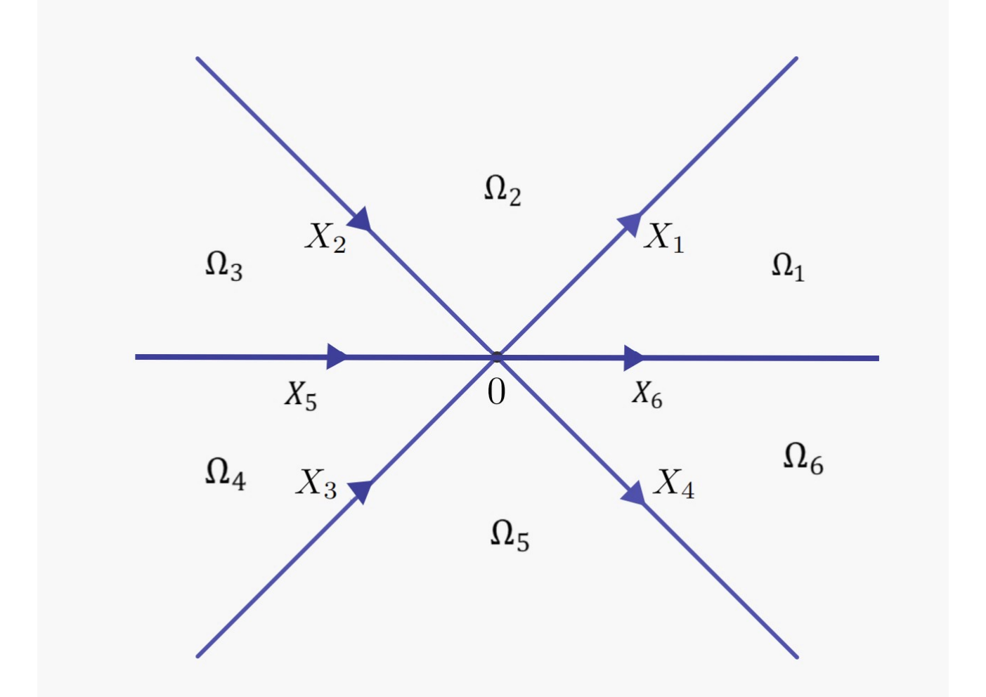
The critical points on $\Sigma$ are illustrated in Figure 1. In fact, the jump matrices $v(x,t,k)$ on each cut have the following symmetries:

v(x,t,k)=\mathcal{A}v(x,t,\omega k)\mathcal{A}^{-1}=\mathcal{B}\overline{v(x,t,\bar{k})}^{-1}\mathcal{B},\ \ k\in\Sigma.

Thus the following transformations focus only on the points $\pm k_{0}$ , furthermore, the other points can be obtained by the above symmetry.

\begin{overpic}[Critical-point.pdf] \end{overpic}

Figure 1. The jump contour

\Sigma

and the critical points

\{\pm k_{0},\pm\omega k_{0},\pm\omega^{2}k_{0}\}

3.1. First transformation

The jump matrices on ${\mathbb{R}}^{+}$ and ${\mathbb{R}}^{-}$ with direction away from the origin are

v_{1}=\left(\begin{array}[]{ccc}1&-r_{1}(k)e^{-\theta_{21}}&0\\ r_{1}^{*}(k)e^{\theta_{21}}&1-\left|r_{1}(k)\right|^{2}&0\\ 0&0&1\end{array}\right),\\

and

v_{4}=\left(\begin{array}[]{ccc}1-\left|r_{2}(k)\right|^{2}&-r_{2}^{*}(k)e^{-\theta_{21}}&0\\ r_{2}(k)e^{\theta_{21}}&1&0\\ 0&0&1\end{array}\right).

The sign diagram of ${\rm Re}(\theta_{21})$ is shown in Fig. 2, where the shaded region denotes ${\rm Re}(\theta_{21})<0$ , while the white region means ${\rm Re}(\theta_{21})>0$ .

\begin{overpic}[sign.pdf] \put(58.6,30.5){\small$k_{0}$} \put(36.3,30.5){\small$-k_{0}$} \end{overpic}

Figure 2. The sign diagram of

{\rm Re}(\theta_{21})

: the shaded region is

{\rm Re}(\theta_{21})<0

and white is

{\rm Re}(\theta_{21})>0

So decompose the jump matrices $v_{1}$ and $v_{4}$ on $0<|k|\leq k_{0}$ , respectively

v_{1}=\left(\begin{array}[]{ccc}1&-r_{1}(k)e^{-\theta_{21}}&0\\ r_{1}^{*}(k)e^{\theta_{21}}&1-\left|r_{1}(k)\right|^{2}&0\\ 0&0&1\end{array}\right)=\left(\begin{array}[]{ccc}1&0&0\\ r_{1}^{*}(k)e^{\theta_{21}}&1&0\\ 0&0&1\end{array}\right)\left(\begin{array}[]{ccc}1&-r_{1}(k)e^{-\theta_{21}}&0\\ 0&1&0\\ 0&0&1\end{array}\right),

and

v_{4}=\left(\begin{array}[]{ccc}1-\left|r_{2}(k)\right|^{2}&-r_{2}^{*}(k)e^{-\theta_{21}}&0\\ r_{2}(k)e^{\theta_{21}}&1&0\\ 0&0&1\end{array}\right)=\left(\begin{array}[]{ccc}1&-r_{2}^{*}(k)e^{-\theta_{21}}&0\\ 0&1&0\\ 0&0&1\end{array}\right)\left(\begin{array}[]{ccc}1&0&0\\ r_{2}(k)e^{\theta_{21}}&1&0\\ 0&0&1\end{array}\right).

However, for $|k|\geq k_{0}$ , a matrix-values function $\Theta$ should be introduced to open lenses naturally. Since the reflect coefficients $r_{1}(k)$ and $r_{2}(k)$ rapidly decay, there exits $\mathcal{C}>0$ such that

|r_{j}(k)|<1,\quad j=1,2,\quad k\in[\mathcal{C},\infty).

Now, let $\delta_{1}(k),\delta_{4}(k)$ be the solution of the scalar RH problem

\left\{\begin{aligned} \delta_{1+}(k)&=\delta_{1-}(k)\left(1-|r_{1}(k)|^{2}\right),&&k\in\Sigma_{1}^{(1)},\\ &=\delta_{1-}(z),&&k\in{\mathbb{C}}\setminus\Sigma_{1}^{(1)},\\ \delta_{1}(k)&\rightarrow 1&&\text{ as }k\rightarrow\infty,\end{aligned}\right.

and

\left\{\begin{aligned} \delta_{4+}(k)&=\delta_{4-}(k)\left(1-|r_{1}(k)|^{2}\right),&&k\in\Sigma_{4}^{(1)},\\ &=\delta_{4-}(z),&&k\in{\mathbb{C}}\setminus\Sigma_{4}^{(1)},\\ \delta_{4}(k)&\rightarrow 1&&\text{ as }k\rightarrow\infty.\end{aligned}\right.

Hence, using the Plemelj formula, it follows that

\delta_{1}(k)=\exp\left\{\frac{1}{2\pi i}\int_{\left[k_{0},\infty\right)}\frac{\ln\left(1-\left|r_{1}(s)\right|^{2}\right)}{s-k}ds\right\},\quad k\in\mathbb{C}\backslash\Sigma_{1}^{(1)},

and

\delta_{4}(k)=\exp\left\{\frac{1}{2\pi i}\int_{[-k_{0},-\infty)}\frac{\ln\left(1-\left|r_{2}(s)\right|^{2}\right)}{s-k}ds\right\},\quad k\in\mathbb{C}\backslash\Sigma_{4}^{(1)}.

Let $\log_{\theta}(k)$ denote the logarithm of $k$ with branch cut along $\arg k=\theta$ , i.e.,

\log_{0}(k)=\ln|k|+\arg_{0}(k),\arg_{0}(k)\in(0,2\pi);\\ \log_{\pi}(k)=\ln|k|+\arg_{\pi}(k),\arg_{\pi}(k)\in(-\pi,\pi).

Proposition 3.1.

The basic properties of $\delta$ functions are given below:

(1). If choosing the branch cut of $\ln$ with $\arg k\in(0,2\pi)$ , the $\delta(k)$ can be rewritten as

\delta_{1}(k)=e^{-i\nu_{1}\log_{0}\left(k-k_{0}\right)}e^{-\chi_{1}(k)}

where

\nu_{1}=-\frac{1}{2\pi}\ln\left(1-\left|r_{1}\left(k_{0}\right)\right|^{2}\right),

and

\chi_{1}(k)=\frac{1}{2\pi i}\int_{k_{0}}^{\infty}\log_{0}(k-s)d\ln\left(1-\left|r_{1}(s)\right|^{2}\right).

Moreover, we have

\delta_{4}(k)=e^{-i\nu_{4}\log_{\pi}\left(k+k_{0}\right)}e^{-\chi_{4}(k)}

with

\nu_{4}=-\frac{1}{2\pi}\ln\left(1-\left|r_{2}\left(-k_{0}\right)\right|^{2}\right),

and

\chi_{4}(k)=\frac{1}{2\pi i}\int_{-k_{0}}^{-\infty}\log_{\pi}(k-s)d\ln\left(1-\left|r_{2}(s)\right|^{2}\right).

(2). The $\delta(k)$ satisfies the conjugate symmetry and are bounded in $|k|>k_{0}$ such that

\delta_{1}(k)={(\overline{\delta_{1}(\bar{k})})^{-1}},\quad k\in\mathbb{C}\backslash\Sigma_{1}^{(1)},\\ \delta_{4}(k)={(\overline{\delta_{4}(\bar{k})})^{-1}},\quad k\in\mathbb{C}\backslash\Sigma_{4}^{(1)},

and

|\delta_{1\pm}(k)|<\infty,\quad{\rm for}~~k>k_{0};\quad|\delta_{4\pm}(k)|<\infty,\quad{\rm for}~~k<-k_{0}.

(3). As $k\to\pm k_{0}$ along with $k>k_{0}$ and $k<-k_{0}$ , respectively, we have

		$\displaystyle\left\|\chi_{1}(k)-\chi_{1}\left(k_{0}\right)\right\|\leq C\left\|k-k_{0}\right\|\left(1+\|\ln\|k-k_{0}\|\|\right),$
		$\displaystyle\left\|\partial_{x}\left(\chi_{1}(k)-\chi_{1}\left(k_{0}\right)\right)\right\|\leq\frac{C}{t}\left(1+\|\ln\|k-k_{0}\|\|\right),$

and

		$\displaystyle\left\|\chi_{4}(k)-\chi_{4}\left(-k_{0}\right)\right\|\leq C\left\|k+k_{0}\right\|\left(1+\|\ln\|k+k_{0}\|\|\right),$
		$\displaystyle\left\|\partial_{x}\left(\chi_{4}(k)-\chi_{4}\left(k_{0}\right)\right)\right\|\leq\frac{C}{t}\left(1+\|\ln\|k+k_{0}\|\|\right).$

Moreover, we have

\begin{gathered}\left|\partial_{x}\chi_{1}\left(k_{0}\right)\right|\leq\frac{C}{t},\quad\partial_{x}\left(\delta_{1}(k)^{\pm 1}\right)=\frac{\pm i\nu}{180tk_{0}^{3}\left(k-k_{0}\right)}\delta_{1}(k)^{\pm 1}.\end{gathered}

Proof.

We focus on the properties of $\delta_{1}$ and the properties of $\delta_{2}$ are similar.

(1). Recall that

\delta_{1}(k)=\exp\left\{\frac{1}{2\pi i}\int_{\left[k_{0},\infty\right)}\frac{\ln\left(1-\left|r_{1}(s)\right|^{2}\right)}{s-k}ds\right\},\quad k\in\mathbb{C}\backslash\Sigma_{1}^{(1)}.

Using the technique of integrations by parts, rewrite the formula of $\delta_{1}$ as follows

	$\displaystyle\delta_{1}(k)$	$\displaystyle=\exp\left\{\frac{1}{2\pi i}\int_{\left[k_{0},\infty\right)}\frac{\ln\left(1-\left\|r_{1}(s)\right\|^{2}\right)}{s-k}ds\right\}=\exp\left\{-\frac{1}{2\pi i}\int_{\left[k_{0},\infty\right)}\frac{\ln\left(1-\left\|r_{1}(s)\right\|^{2}\right)}{k-s}ds\right\}$
		$\displaystyle=\exp\left\{\frac{1}{2\pi i}\int_{\left[k_{0},\infty\right)}{\ln\left(1-\left\|r_{1}(s)\right\|^{2}\right)}d\ (\ln(k-s))\right\}$
		$\displaystyle=\exp\left\{\frac{1}{2\pi i}\left({\ln\left(1-\left\|r_{1}(s)\right\|^{2}\right)}\ln(k-s)\|_{k_{0}}^{\infty}-\int_{\left[k_{0},\infty\right)}\ln(k-s)d\ {\ln\left(1-\left\|r_{1}(s)\right\|^{2}\right)}\right)\right\}$
		$\displaystyle=\exp\left\{\frac{1}{2\pi i}\left(-{\ln\left(1-\left\|r_{1}(k_{0})\right\|^{2}\right)}\log_{0}(k-k_{0})-\int_{\left[k_{0},\infty\right)}\log_{0}(k-s)d\ {\ln\left(1-\left\|r_{1}(s)\right\|^{2}\right)}\right)\right\}$
		$\displaystyle=e^{-i\nu_{1}\log_{0}(k-k_{0})}e^{-\chi_{1}(k)},$

where we have chosen the branch cut $0<\arg(k-k_{0})<2\pi$ , since the jump contour is $k>k_{0}$ .

(2). By using the uniqueness of RH problem of $\delta_{1}(k)$ , it is found that $\overline{\delta_{1}(\bar{k})}^{-1}$ satisfies the same RH problem, so that $\delta_{1}(k)=\overline{\delta_{1}(\bar{k})}^{-1}$ . When $k_{0}$ large enough, the reflection coefficients is strictly small than $1$ and inserting the symmetry of $\delta_{1}(k)$ yields

	$\displaystyle\delta_{1+}(k)$	$\displaystyle=\delta_{1-}(k)\left(1-\|r_{1}(k)\|^{2}\right),$
		$\displaystyle=\overline{\delta_{1-}(\bar{k})}^{-1}\left(1-\|r_{1}(k)\|^{2}\right),$
		$\displaystyle=\overline{\delta_{1+}(k)}^{-1}\left(1-\|r_{1}(k)\|^{2}\right),$
	$\displaystyle\|\delta_{1+}(k)\|^{2}$	$\displaystyle=\left(1-\|r_{1}(k)\|^{2}\right),$

and the same procedure leads to

|\delta_{1-}|^{2}\leq\left(1-\sup_{k_{0}\in[c_{0},M]}|r_{1}(k_{0})|^{2}\right)^{-1}.

In conclusion, $|\delta_{1\pm}|$ is bounded and hence, by the maximum principle $|\delta_{1}(k)|$ is bounded. Finally, using the fact of symmetry, it is concluded that $|\delta_{1}^{-1}(k)|$ is bounded.

(3). The facts that $r_{1}(k)$ rapidly decays and the integral of $\log_{0}(k)$ is well defined near the zero indicate that for any $\epsilon>0$ one can estimate $\chi_{1}(k_{0})$ as

	$\displaystyle\|\chi_{1}(k)-\chi_{1}(k_{0})\|$	$\displaystyle=\left\|\frac{1}{2\pi i}\int_{k_{0}}^{\infty}\log_{0}(k-s)-\log_{0}(k_{0}-s)d\ln\left(1-\left\|r_{1}(s)\right\|^{2}\right)\right\|$
		$\displaystyle\leq C\int_{k_{0}}^{k_{0}+\epsilon}\left\|\log_{0}(k-s)-\log_{0}(k_{0}-s)\right\|\|d\ln\left(1-\left\|r_{1}(s)\right\|^{2}\right)\|$
		$\displaystyle+\int_{k_{0}+\epsilon}^{\infty}\left\|\log_{0}(k-s)-\log_{0}(k_{0}-s)\right\|\|d\ln\left(1-\left\|r_{1}(s)\right\|^{2}\right)\|,$

where for the first term, we have

		$\displaystyle\int_{k_{0}}^{k_{0}+\epsilon}\left\|\log_{0}(k-s)-\log_{0}(k_{0}-s)\right\|\|d\ln\left(1-\left\|r_{1}(s)\right\|^{2}\right)\|$
		$\displaystyle=\int_{k_{0}}^{k_{0}+\epsilon}\left\|\log_{0}(k-s)-\log_{0}(k_{0}-s)\right\|\frac{\partial_{s}\|r_{1}(s)\|}{1-\left\|r_{1}(s)\right\|^{2}}ds$
		$\displaystyle\leq\\|\frac{\partial_{s}\|r_{1}(s)\|}{1-\left\|r_{1}(s)\right\|^{2}}\\|_{L^{\infty}(k_{0},k_{0}+\epsilon)}\int_{k_{0}}^{k_{0}+\epsilon}\left\|\log_{0}(k-s)-\log_{0}(k_{0}-s)\right\|ds$
		$\displaystyle\leq C\|\left((s-k_{0})\log_{0}(s-k_{0})+(k_{0}-s)\|_{k_{0}}^{k_{0}+\epsilon}\right)-\left((s-k)\log_{0}(s-k)+(k-s)\|_{k_{0}}^{k_{0}+\epsilon}\right)\|$
		$\displaystyle=C\|\epsilon log_{0}(\epsilon)-\epsilon-(k_{0}-k+\epsilon)\log_{0}(k_{0}-k+\epsilon)+(k_{0}-k+\epsilon)+(k_{0}-k)\log_{0}(k_{0}-k)-(k_{0}-k)\|$
		$\displaystyle\leq\|k_{0}-k\|(1+\|ln(k-k_{0})\|).$

and for the second term

		$\displaystyle\int_{k_{0}+\epsilon}^{\infty}\left\|\log_{0}(k-s)-\log_{0}(k_{0}-s)\right\|\|d\ln\left(1-\left\|r_{1}(s)\right\|^{2}\right)$
		$\displaystyle\leq\|k-k_{0}\|\int_{k_{0}+\epsilon}^{\infty}\|\frac{1}{\eta-s}\|d\ln\left(1-\left\|r_{1}(s)\right\|^{2}\right)\leq\|k-k_{0}\|(1+\ln(k_{0}-k)).$

Furthermore, for the critical point $k_{0}=\sqrt[4]{\frac{x}{45t}}$ , by the estimates above and taking the derivative with respect to $x$ , one can get the estimate for $\partial_{x}\chi(k)$ .

Using the symmetry properties, and considering $\delta_{1}$ and $\delta_{4}$ , define $\delta_{j}~(j=2,3,5,6)$ as follows

\begin{array}[]{ll}\delta_{3}(k)=\delta_{1}\left(\omega^{2}k\right),&k\in\mathbb{C}\backslash\Sigma_{3}^{(1)},\\ \delta_{5}(k)=\delta_{1}(\omega k),&k\in\mathbb{C}\backslash\Sigma_{5}^{(1)},\\ \delta_{2}(k)=\delta_{4}\left(\omega^{2}k\right),&k\in\mathbb{C}\backslash\Sigma_{2}^{(1)},\\ \delta_{6}(k)=\delta_{4}(\omega k),&k\in\mathbb{C}\backslash\Sigma_{6}^{(1)},\end{array}

which satisfy the jump conditions

\begin{array}[]{ll}\delta_{3+}(k)=\delta_{3-}(k)\left(1-\left|r_{1}\left(\omega^{2}k\right)\right|^{2}\right),&k\in\Sigma_{3}^{(1)},\\ \delta_{5+}(k)=\delta_{5-}(k)\left(1-\left|r_{1}(\omega k)\right|^{2}\right),&k\in\Sigma_{5}^{(1)},\\ \delta_{2+}(k)=\delta_{2-}(k)\left(1-\left|r_{2}\left(\omega^{2}k\right)\right|^{2}\right),&k\in\Sigma_{2}^{(1)},\\ \delta_{6+}(k)=\delta_{6-}(k)\left(1-\left|r_{2}(\omega k)\right|^{2}\right),&k\in\Sigma_{6}^{(1)}.\end{array}

∎

Remark 3.2.

The function $\ln(k)$ in $\delta_{n}(k)$ selects the branch cut $\frac{(n-1)\pi}{3}<\arg(k)<2\pi+\frac{(n-1)\pi}{3}$ for $n=1,2,3$ and the branch cut $-\frac{(7-n)\pi}{3}<\arg(k)<2\pi-\frac{(7-n)\pi}{3}$ for $n=4,5,6$ .

Thus define the matrix function $\Theta(k)$ to factorize the RH problem. In particular,

M^{(1)}(x,t,k)=M(x,t,k)\Theta(k),

where $\Theta(k)$ is

\Theta(k)=\left(\begin{array}[]{ccc}\frac{\delta_{1}(k)\delta_{6}(k)}{\delta_{3}(k)\delta_{4}(k)}&0&0\\ 0&\frac{\delta_{5}(k)\delta_{4}(k)}{\delta_{1}(k)\delta_{2}(k)}&0\\ 0&0&\frac{\delta_{3}(k)\delta_{2}(k)}{\delta_{5}(k)\delta_{6}(k)}\end{array}\right)=\left(\begin{array}[]{ccc}\Theta_{1}(k)&0&0\\ 0&\Theta_{2}(k)&0\\ 0&0&\Theta_{3}(k)\end{array}\right)

with $\Theta(k)=I+O\left(k^{-1}\right)\text{as}k\rightarrow\infty$ .

The jump matrix is $v^{(1)}(x,t;k)=\Theta^{-1}_{-}v(x,t;k)\Theta_{+}$ , and one can get for $|k|>k_{0}$ as follows

	$\displaystyle v_{1}^{(1)}$	$\displaystyle=\left(\begin{array}[]{ccc}\frac{\Theta_{1+}}{\Theta_{1-}}&-\frac{\Theta_{2+}}{\Theta_{1-}}r_{1}(k)e^{-t\Phi_{21}}&0\\ \frac{\Theta_{1+}}{\Theta_{2-}}r_{1}^{}(k)e^{t\Phi_{21}}&\frac{\Theta_{2}-}{\Theta_{2+}}\left(1-r_{1}(k)r_{1}^{}(k)\right)&0\\ 0&0&1\end{array}\right)=\left(\begin{array}[]{ccc}\frac{\delta_{1+}}{\delta_{1-}}&-\frac{\tilde{\delta}_{v_{1}}}{\delta_{1-}\delta_{1+}}r_{1}(k)e^{-t\Phi_{21}}&0\\ \frac{\delta_{1+}\delta_{1-}}{\tilde{\delta}_{v_{1}}}r_{1}^{}(k)e^{t\Phi_{21}}&\frac{\delta_{1-}}{\delta_{1+}}\left(1-r_{1}(k)r_{1}^{}(k)\right)&0\\ 0&0&1\end{array}\right)$
		$\displaystyle=\left(\begin{array}[]{ccc}1-\|r_{1}(k)\|^{2}&-\frac{\tilde{\delta}_{v_{1}}}{\delta_{1-}^{2}}\frac{r_{1}(k)}{1-\|r_{1}(k)\|^{2}}e^{-t\Phi_{21}}&0\\ \frac{\delta_{1+}^{2}}{\tilde{\delta}_{v_{1}}}\frac{r_{1}^{*}(k)}{1-\|r_{1}(k)\|^{2}}e^{t\Phi_{21}}&1&0\\ 0&0&1\end{array}\right),$

and

v_{4}^{(1)}=\left(\begin{array}[]{ccc}1&-\frac{\delta_{4+}^{2}}{\tilde{\delta}_{v_{4}}}\frac{r_{2}^{*}(k)}{1-|r_{2}(k)|^{2}}e^{-t\Phi_{21}}&0\\ \frac{\tilde{\delta}_{v_{4}}}{\delta_{4-}^{2}}\frac{r_{2}(k)}{1-|r_{2}(k)|^{2}}e^{t\Phi_{21}}&1-\left|r_{2}(k)\right|^{2}&0\\ 0&0&1\end{array}\right),

where $\tilde{\delta}_{v_{1}}=\frac{\delta_{3}\delta^{2}_{4}\delta_{5}}{\delta_{6}\delta_{2}}$ and $\tilde{\delta}_{v_{4}}=\frac{\delta_{1}^{2}\delta_{2}\delta_{6}}{\delta_{5}\delta_{3}}$ .

Furthermore, the other jump matrices can be obtained by the symmetry or direct calculations:

		$\displaystyle v_{3}^{(1)}=\left(\begin{array}[]{ccc}1&0&\frac{\delta_{3+}^{2}}{\tilde{\delta}_{v_{3}}}\frac{r_{1}^{}\left(\omega^{2}k\right)}{1-r_{1}\left(\omega^{2}k\right)r_{1}^{}\left(\omega^{2}k\right)}e^{-\theta_{31}}\\ 0&1&0\\ -\frac{\tilde{\delta}_{v_{3}}}{\delta_{3-}^{2}}\frac{r_{1}\left(\omega^{2}k\right)}{1-r_{1}\left(\omega^{2}k\right)r_{1}^{}\left(\omega^{2}k\right)}e^{\theta_{31}}&0&1-r_{1}\left(\omega^{2}k\right)r_{1}^{}\left(\omega^{2}k\right)\end{array}\right),$
		$\displaystyle v_{5}^{(1)}=\left(\begin{array}[]{ccc}1&0&0\\ 0&1-r_{1}(\omega k)r_{1}^{}(\omega k)&-\frac{\tilde{\delta}_{v_{5}}}{\delta_{5-}^{2}}\frac{r_{1}(\omega k)}{1-r_{1}(\omega k)r_{1}^{}(\omega k)}e^{-\theta_{32}}\\ 0&\frac{\delta_{5+}^{2}}{\tilde{\delta}_{v_{5}}}\frac{r_{1}^{}(\omega k)}{1-r_{1}(\omega k)r_{1}^{}(\omega k)}e^{\theta_{32}}&1\end{array}\right),$

and

		$\displaystyle v_{2}^{(1)}=\left(\begin{array}[]{ccc}1&0&0\\ 0&1&-\frac{\delta_{2+}^{2}}{\tilde{\delta}_{v_{2}}}\frac{r_{2}^{}(\omega k)}{1-r_{2}(\omega k)r_{2}^{}(\omega k)}e^{-\theta_{32}}\\ 0&\frac{\tilde{\delta}_{v_{2}}}{\delta_{2-}^{2}}\frac{r_{2}(\omega k)}{1-r_{2}(\omega k)r_{2}^{}(\omega k)}e^{\theta_{32}}&1-r_{2}(\omega k)r_{2}^{}(\omega k)\end{array}\right),$
		$\displaystyle v_{6}^{(1)}=\left(\begin{array}[]{ccc}1-r_{2}\left(\omega^{2}k\right)r_{2}^{}\left(\omega^{2}k\right)&0&\frac{\tilde{\delta}_{v_{6}}}{\delta_{6-}^{2}}\frac{r_{2}\left(\omega^{2}k\right)}{1-r_{2}\left(\omega^{2}k\right)r_{2}^{}\left(\omega^{2}k\right)}e^{-\theta_{31}}\\ 0&1&0\\ -\frac{\delta_{6+}^{2}}{\tilde{\delta}_{v_{6}}}\frac{r_{2}^{}\left(\omega^{2}k\right)}{1-r_{2}\left(\omega^{2}k\right)r_{2}^{}\left(\omega^{2}k\right)}e^{\theta_{31}}&0&1\end{array}\right).$

On the other hand, since on the $\Sigma_{j=7,8,\cdots,12}$ the $\delta_{j}$ has no jump, the jump matrix $v_{\{j=7,8,\cdots,12\}}$ are just as follows

v_{7}^{(1)}=\left(\begin{array}[]{ccc}\frac{\Theta_{1+}}{\Theta_{1-}}&-\frac{\Theta_{2+}}{\Theta_{1-}}r_{1}(k)e^{-t\Phi_{21}}&0\\ \frac{\Theta_{1+}}{\Theta_{2-}}r_{1}^{*}(k)e^{t\Phi_{21}}&\frac{\Theta_{2}-}{\Theta_{2+}}\left(1-r_{1}(k)r_{1}^{*}(k)\right)&0\\ 0&0&1\end{array}\right)\\ =\left(\begin{array}[]{ccc}1&-\frac{\tilde{\delta}_{v1}}{\delta_{1}^{2}}r_{1}(k)e^{-t\Phi_{21}}&0\\ \frac{\delta_{1}^{2}}{\tilde{\delta}_{v1}}r_{1}^{*}(k)e^{t\Phi_{21}}&1-r_{1}(k)r_{1}^{*}(k)&0\\ 0&0&1\end{array}\right),\\

and

v_{9}^{(1)}=\left(\begin{array}[]{ccc}1-r_{1}\left(\omega^{2}k\right)r_{1}^{*}\left(\omega^{2}k\right)&0&\frac{\delta_{3}^{2}}{\tilde{\delta}_{v_{3}}}r_{1}^{*}\left(\omega^{2}k\right)e^{-\theta_{31}}\\ 0&1&0\\ -\frac{\tilde{\delta}_{v_{3}}}{\delta_{3}^{2}}r_{1}\left(\omega^{2}k\right)e^{\theta_{31}}&0&1\end{array}\right)\\ v_{11}^{(1)}=\left(\begin{array}[]{ccc}1&0&0\\ 0&1&-\frac{\tilde{\delta}_{v_{5}}}{\delta_{5}^{2}}{r_{1}(\omega k)}e^{-\theta_{32}}\\ 0&\frac{\delta_{5}^{2}}{\tilde{\delta}_{v_{5}}}{r_{1}^{*}(\omega k)}e^{\theta_{32}}&1-r_{1}(\omega k)r_{1}^{*}(\omega k)\end{array}\right).

Moreover, one has

v_{8}^{(1)}=\left(\begin{array}[]{ccc}1&0&0\\ 0&1-r_{2}(\omega k)r_{2}^{*}(\omega k)&-\frac{\delta_{2}^{2}}{\tilde{\delta}_{v_{2}}}{r_{2}^{*}(\omega k)}e^{-\theta_{32}}\\ 0&\frac{\tilde{\delta}_{v_{2}}}{\delta_{2}^{2}}{r_{2}(\omega k)}e^{\theta_{32}}&1\end{array}\right),\\ v_{10}^{(1)}=\left(\begin{array}[]{ccc}1-\left|r_{2}(k)\right|^{2}&-\frac{\delta_{4}^{2}}{\tilde{\delta}_{v_{4}}}{r_{2}^{*}(k)}e^{-t\Phi_{21}}&0\\ \frac{\tilde{\delta}_{v_{4}}}{\delta_{4}^{2}}{r_{2}(k)}e^{t\Phi_{21}}&1&0\\ 0&0&1\end{array}\right),

v_{12}^{(1)}=\left(\begin{array}[]{ccc}1&0&\frac{\tilde{\delta}_{v_{6}}}{\delta_{6}^{2}}{r_{2}\left(\omega^{2}k\right)}\\ 0&1&0\\ -\frac{\delta_{6}^{2}}{\tilde{\delta}_{v_{6}}}{r_{2}^{*}\left(\omega^{2}k\right)}e^{\theta_{31}}&0&1-\left|r_{2}(k)\right|^{2}\end{array}\right).

Next, suppose

\rho_{1}(k)=\frac{r_{1}(k)}{1-r_{1}(k)r_{1}^{*}(k)},\quad\rho_{2}(k)=\frac{r_{2}(k)}{1-r_{2}(k)r_{2}^{*}(k)}.

It is necessary to decompose the functions $r_{j},r_{j}^{*}$ and $\rho_{j}(k)$ for analytic extension.

Lemma 3.3.

The functions $r_{j}$ and $\rho_{j}~(j=1,2)$ have the following decompositions

\begin{array}[]{ll}r_{1}(k)=r_{1,a}(x,t,k)+r_{1,r}(x,t,k),&k\in\left[0,k_{0}\right],\\ r_{2}^{*}(k)=r_{2,a}^{*}(x,t,k)+r_{2,r}^{*}(x,t,k),&k\in[-k_{0},0],\\ \rho_{1}(k)=\rho_{1,a}(x,t,k)+\rho_{1,r}(x,t,k),&k\in\left[k_{0},\infty\right),\\ \rho_{2}^{*}(k)=\rho_{2,a}^{*}(x,t,k)+\rho_{2,r}^{*}(x,t,k),&k\in\left(-\infty,k_{0}\right].\end{array}

Fig. 3 shows the sign diagram of ${\rm Re}(\Phi_{21})$ , where $U_{1}\cup U_{3}\cup U_{5}=\{k:{\rm Re}(\Phi_{21})<0\}$ and $U_{2}\cup U_{4}\cup U_{6}=\{k:{\rm Re}(\Phi_{21})>0\}$ .

\begin{overpic}[sign.pdf] \put(63.6,37.9){\small$U_{1}$} \put(48.5,37.9){\small$U_{2}$} \put(33.5,37.9){\small$U_{3}$} \put(63.6,30.3){\small$U_{6}$} \put(48.5,30.3){\small$U_{5}$} \put(33.5,30.3){\small$U_{4}$} \end{overpic}

Figure 3. The shaded region is

{\rm Re}(\Phi_{21})<0

and white is

{\rm Re}(\Phi_{21})>0

Furthermore, the decomposition functions have the following properties:

(1). For $0<k_{0}<M$ , $r_{1,a}$ and $r_{2,a}^{*}$ are defined and continuous for $k\in\bar{U}_{2}$ and analytic for $k\in U_{2}$ , but the domain for $r_{1,a},r_{2,a}^{*}$ are restricted by $0\leq\operatorname{Re}(k)\leq k_{0}$ and $-k_{0}\leq\operatorname{Re}(k)\leq 0$ , respectively. The function $\rho_{1,a}^{*}$ is defined and continuous for $k\in\bar{U}_{1}$ and analytic for $k\in U_{1}$ , $\rho_{2,a}$ are defined and continuous for $k\in\bar{U}_{3}$ and analytic for $k\in U_{3}$ .

(2). For $0<k_{0}<M$ , the functions $r_{1,a},r_{2,a}^{*}$ and $\rho_{1,a}^{*},\rho_{2,a}$ satisfy the following estimates:

\left|\partial_{x}^{l}(r_{1,a}(x,t,k)-r_{1}(0))\right|\leq C|k|{e^{-t\operatorname{Re}\Phi_{21}(k)/2}},\quad k\in\bar{U}_{2}~\text{and}~{\rm Re}(k)\in[0,k_{0}];\\

\left|\partial_{x}^{l}(r_{1,a}(x,t,k)-r_{1}(k_{0}))\right|\leq C|k-k_{0}|{e^{-t\operatorname{Re}\Phi_{21}(k)/2}},\quad k\in\bar{U}_{2}\ \text{and}~{\rm Re}(k)\in[0,k_{0}];\\

and

\left|\partial_{x}^{l}(r_{2,a}^{*}(x,t,k)-r_{2}^{*}(0))\right|\leq C|k|{e^{-t\operatorname{Re}\Phi_{21}(k)/2}},\quad k\in\bar{U}_{2}~\text{and}~\operatorname{Re}(k)\in[-k_{0},0];\\

\left|\partial_{x}^{l}(r_{2,a}^{*}(x,t,k)-r_{2}^{*}(-k_{0}))\right|\leq C|k+k_{0}|{e^{-t\operatorname{Re}\Phi_{21}(k)/2}},\quad k\in\bar{U}_{2}\ \text{and}\ \operatorname{Re}(k)\in[-k_{0},0].\\

Furthermore,

\left|\partial_{x}\rho_{1,a}(x,t,k)\right|\leq\frac{Ce^{-t\operatorname{Re}\Phi_{21}(k)/2}}{1+|k|}\quad k\in\bar{U}_{6},\\ \left|\partial_{x}(\rho_{1,a}(x,t,k)-\rho_{1}(k_{0}))\right|\leq{C|k-k_{0}|e^{-t\operatorname{Re}\Phi_{21}(k)/2}}\quad k\in\bar{U}_{6}.

and

\left|\partial_{x}\rho_{2,a}(x,t,k)\right|\leq\frac{Ce^{t\operatorname{Re}\Phi_{21}(k)/2}}{1+|k|}\quad k\in\bar{U}_{3},\\ \left|\partial_{x}(\rho_{2,a}(x,t,k)-\rho_{2}(-k_{0}))\right|\leq{C|k+k_{0}|e^{t\operatorname{Re}\Phi_{21}(k)/2}}\quad k\in\bar{U}_{3}.

(3). For $0<k_{0}<M$ and $1\leq p\leq\infty$ , the functions $r_{j,r}$ and $\rho_{j,r}$ satisfy

\left\|\partial_{x}^{l}r_{1,r}(x,t,k)e^{-t\Phi_{21}}\right\|_{L^{p}{(0,k_{0})}}\leq\frac{c}{t^{3/2}}\quad 0<k<k_{0},\\ \left\|\partial_{x}^{l}r_{2,r}^{*}(x,t,k)e^{-t\Phi_{21}}\right\|_{L^{p}(-k_{0},0)}\leq\frac{c}{t^{3/2}}\quad-k_{0}<k<0,

and

\left\|(1+|\cdot|)\partial_{x}^{l}\rho_{1,r}(x,t,\cdot)e^{-t\Phi_{21}}\right\|_{L^{p}[k_{0},\infty)}\leq\frac{c}{t^{3/2}},\\ \left\|(1+|\cdot|)\partial_{x}^{l}\rho_{2,r}(x,t,\cdot)e^{t\Phi_{21}}\right\|_{L^{p}(-\infty,-k_{0}]}\leq\frac{c}{t^{3/2}}.

Proof.

Recall that the reflection coefficient $r_{1}(k)$ is smooth for $k\in[0,\infty)$ , so that we can take Taylor expansion about $r_{1}(k)$ near $k_{0}$ point:

r_{1}(k)=r_{1}(k_{0})+\partial_{k}r_{1}|_{k=k_{0}}(k-k_{0})+\cdots+\frac{1}{n!}\int_{k_{0}}^{k}\partial_{k}^{(n+1)}r_{1}(\tau)(k-\tau)^{n}d\tau.

Let $R(k)=\sum_{i=0}^{n}\partial_{k}^{i}r_{1}|_{k=k_{0}}(k-k_{0})^{i}$ and $h(k):=r_{1}(k)-R(k)$ , now we split the $h(k)$ into $h(k)=h_{1}(k)+h_{2}(k)$ .

Set

\beta(k)=(k-k_{0})^{q}.

Rewrite $\theta_{21}$ as

\theta_{21}=2it\left(\frac{9\sqrt{3}k^{5}-\sqrt{3}k\xi}{2}\right):=2it\theta(\xi,k)

For $k\in[0,k_{0}]$ , As $k\to\theta(\xi,k)$ is one-to-one, we define

\left\{\begin{aligned} \frac{h}{\beta}(\theta)&:=\frac{h(\theta(k))}{\beta(\theta(k))},&&-18\sqrt{3}k_{0}^{5}=\theta(k_{0})<\theta<0,\\ &:=0,&&\text{Otherwise}.\end{aligned}\right.

And rewrite $h(k)$ as

	$\displaystyle h(k)$	$\displaystyle=\frac{1}{n!}\int_{k_{0}}^{k}\partial_{k}^{(n+1)}r_{1}(\tau)(k-\tau)^{n}d\tau$
		$\displaystyle=\frac{(k-k_{0})^{n+1}}{n!}\int_{0}^{1}\partial_{k}^{(n+1)}r_{1}(k_{0}+\mu(k-k_{0}))(1-\mu)^{n}d\mu$

then

\frac{h}{\beta}(\theta)=(k-k_{0})^{n-q+1}g(k_{0},k),\quad\theta(k_{0})<\theta<0,

where

g(k_{0},k)=\frac{1}{n!}\int_{0}^{1}\partial_{k}^{(n+1)}r_{1}(k_{0}+\mu(k-k_{0}))(1-\mu)^{n}d\mu.

Since the reflect coefficient $r_{1}$ belong to Schwartz space, so that $|\partial_{k}g(k_{0},k)|\leq\infty$ , and as $\frac{dk}{d\theta}=\frac{2}{45\sqrt{3}(k^{4}-k_{0}^{4})}$ and $0<k_{0}<M$ , we can estimate that

	$\displaystyle\int_{0}^{k_{0}}\left\|\left(\frac{d}{d\theta}\right)^{j}\frac{h}{\beta}(k)\right\|^{2}\|\bar{d}\theta(k)\|$	$\displaystyle\leq C\int_{0}^{k_{0}}\left\|\left(\frac{d}{dk}\frac{1}{\|k^{4}-k_{0}^{4}\|}\right)^{j}\frac{h}{\beta}(k)\right\|^{2}\|k^{4}-k_{0}^{4}\|\bar{d}k$
		$\displaystyle=C\int_{0}^{k_{0}}\left\|\left(\frac{1}{\|k^{4}-k_{0}^{4}\|}\frac{d}{dk}\right)^{j}(k-k_{0})^{n-q+1}g(k_{0},k)\right\|^{2}\|k^{4}-k_{0}^{4}\|\bar{d}k$
		$\displaystyle\leq C\int_{0}^{k_{0}}\left\|(k-k_{0})^{2n-2q-4j+3}\right\|\bar{d}k<\infty,$

for the $0\leq j\leq\frac{2n-2q+4}{4}$ .

Thus one can conclude that $\frac{h}{\beta}(\theta)\in H^{j}({\mathbb{R}})$ for $0\leq j\leq\frac{2n-2q+4}{4}$ , and one can define the Fourier inversion transform

\frac{h}{\beta}(k)=\int_{-\infty}^{\infty}e^{is\theta(k)}\widehat{\left(\frac{h}{\beta}\right)}(s)\bar{d}s,\quad k\in[0,k_{0}],

where

\widehat{\left(\frac{h}{\beta}\right)}(s)=-\int_{0}^{k_{0}}e^{-is\theta(k)}\left(\frac{h}{\beta}\right)(k)\bar{d}\theta(k),\quad s\in{\mathbb{R}}.

Because $\frac{h}{\beta}(\theta)\in H^{j}({\mathbb{R}})$ and by the Plancherel formula, we have that

\int_{-\infty}^{\infty}(1+s^{2})^{j}\left|\widehat{\left(\frac{h}{\beta}\right)}(s)\right|^{2}ds\leq C.

Now split the $h(k)$ as

{h}(k)={\beta}(k)\int_{t}^{\infty}e^{is\theta(k)}\widehat{\left(\frac{h}{\beta}\right)}(s)\bar{d}s+{\beta}(k)\int_{-\infty}^{t}e^{is\theta(k)}\widehat{\left(\frac{h}{\beta}\right)}(s)\bar{d}s\\ :=h_{1}(k)+h_{2}(k),\quad k\in[0,k_{0}].

Then for $k\in[0,k_{0}]$ , one has

\begin{split}\begin{aligned} |e^{-2it\theta(k)}h_{1}(k)|&=\left|e^{-2it\theta(k)}{\beta}(k)\int_{t}^{\infty}e^{is\theta(k)}\widehat{\left(\frac{h}{\beta}\right)}(s)\bar{d}s\right|\\ &\leq\left|e^{-it\theta(k)}{\beta}(k)\right|\int_{t}^{\infty}\left|e^{i(s-t)\theta(k)}\widehat{\left(\frac{h}{\beta}\right)}(s)\right|\bar{d}s\\ &=|\beta(k)|\int_{t}^{\infty}\left|\widehat{\left(\frac{h}{\beta}\right)}(s)\right|\bar{d}s\\ &\leq C\left(\int_{t}^{\infty}\left|(1+s^{2})^{j}\widehat{\left(\frac{h}{\beta}\right)}(s)\right|^{2}ds\right)^{\frac{1}{2}}\left(\int_{t}^{\infty}\left|(1+s^{2})^{-j}\right|^{2}ds\right)^{\frac{1}{2}}\\ &\leq\frac{C}{t^{j-\frac{1}{2}}}.\end{aligned}\end{split}

(3.3)

On the other hand, for $k\in U_{2}$ and $\operatorname{Re}(k)\in[0,k_{0}]$ , we have

	$\displaystyle\|e^{-2it\theta(k)}h_{2}(k)\|$	$\displaystyle=\left\|e^{-2it\theta(k)}{\beta}(k)\int_{-\infty}^{t}e^{is\theta(k)}\widehat{\left(\frac{h}{\beta}\right)}(s)\bar{d}s\right\|$
		$\displaystyle=\left\|e^{-it\theta(k)}{\beta}(k)\int_{-\infty}^{t}e^{i(s-t)\theta(k)}\widehat{\left(\frac{h}{\beta}\right)}(s)\bar{d}s\right\|$
		$\displaystyle\leq C\left\|e^{-it\theta(k)}{\beta}(k)\right\|\int_{-\infty}^{t}e^{(s-t)\operatorname{Re}(i\theta(k))}\left\|\widehat{\left(\frac{h}{\beta}\right)}(s)\right\|ds$
		$\displaystyle\leq Ce^{-t\operatorname{Re}(i\theta(k))}.$

Moreover, by directly computation one can get $|e^{-2it\theta(k)}R(k)|\leq Ce^{-2t\operatorname{Re}(i\theta(k))}$ , for $k\in U_{2}$ and $\operatorname{Re}(k)\in[0,k_{0}]$ .

Finally, we can define $r_{1,a}(k):=h_{2}(k)+R(k)$ which can be analytically extent to the $U_{2}$ with $\operatorname{Re}(k)\in[0,k_{0}]$ and $r_{1,r}(k):=h_{1}(k)$ define on $0\leq k\leq k_{0}$ .

Take $n=2,q=1$ for the estimate above, then we can get that

R(k)=r_{1}(k_{0})+\partial_{k}r_{1}(k_{0})(k-k_{0})+\partial_{k}^{2}r_{1}(k_{0})(k-k_{0})^{2},\\ h_{2}(k)=(k-k_{0})\int_{-\infty}^{t}e^{is\theta(k)}\widehat{\left(\frac{h}{\beta}\right)}(s)\bar{d}s,

moreover,

|r_{1,a}(k)-r_{1}(k_{0})|\leq C|k-k_{0}|e^{-\operatorname{Re}\theta_{21}(k)}.

By the directly computation, one can get

|\partial_{x}(r_{1,a}(k)-r_{1}(0))|\leq C|k-k_{0}|e^{-\operatorname{Re}\theta_{21}(k)}.

The estimate between $r_{1,a}(k)$ and $r_{1}(0)$ need us to make Taylor expansion near $k=0$ , the procedure is similar, so we omitted it.

Again, by the Taylor’s expansion, we have that

(k+i)^{n+5}\rho_{1}^{*}(k)=\gamma_{0}+\gamma_{1}(k-k_{0})+\cdots+\gamma_{n}(k-k_{0})^{n}+\frac{1}{n!}\int_{k_{0}}^{k}((\cdot+i)\rho_{1}(\cdot))^{(n+1)}(\mu)(k-\mu)^{n}d\mu,

and define

R(k)=\frac{\sum_{i=0}^{n}\gamma_{i}(k-k_{0})^{i}}{(k+i)^{n+5}},h(k)=\rho_{1}^{*}(k)-R(k).

Set

\beta(k)=\frac{(k-k_{0})^{q}}{(k+i)^{q+2}}.

By the Fourier transform

\frac{h}{\beta}=\int_{-\infty}^{\infty}e^{is\theta(k)}\widehat{\left(\frac{h}{\beta}\right)}(s)\bar{d}s,

where

\widehat{\frac{h}{\beta}}(s)=\int_{k_{0}}^{\infty}e^{-is\theta(k)}{\left(\frac{h}{\beta}\right)}(k)\bar{d}\theta(k).

As the same procedure, we estimate that

\frac{h}{\beta}=\frac{(k-k_{0})^{n-q+1}}{(k+i)^{n-q+3}}g(k_{0};k).

Here

g(k_{0},k)=\frac{1}{n!}\int_{0}^{1}((\cdot+i)^{n+5}\rho_{1}(\cdot))^{(n+1)}(k_{0}+\mu(k-k_{0}))(1-\mu)^{n}d\mu

and $|\partial_{k}g(k_{0},k)|<\infty$ .

Now, we obtain that

	$\displaystyle\int_{k_{0}}^{\infty}\left\|\left(\frac{d}{d\theta}\right)^{j}\frac{h}{\beta}(k)\right\|^{2}\|\bar{d}\theta(k)\|$	$\displaystyle\leq C\int_{k_{0}}^{\infty}\left\|\left(\frac{d}{dk}\frac{1}{\|k^{4}-k_{0}^{4}\|}\right)^{j}\frac{h}{\beta}(k)\right\|^{2}\|k^{4}-k_{0}^{4}\|\bar{d}k$
		$\displaystyle=C\int_{k_{0}}^{\infty}\left\|\left(\frac{1}{\|k^{4}-k_{0}^{4}\|}\frac{d}{dk}\right)^{j}\frac{(k-k_{0})^{n-q+1}}{(k+i)^{n-q+3}}g(k_{0},k)\right\|^{2}\|k^{4}-k_{0}^{4}\|\bar{d}k$
		$\displaystyle\leq C\int_{k_{0}}^{\infty}\left\|\frac{(k-k_{0})^{2n-2q-4j+3}}{(k+i)^{2n-2q+6}}\right\|\bar{d}k<\infty,$

for $j\leq\frac{n-q+2}{2}$ , and we can conclude that $\frac{h}{\beta}\in H^{j}(k_{0},\infty]$ .

By the Plancherel formula, we can get that

\int_{-\infty}^{\infty}(1+s^{2})^{j}\left|\widehat{\left(\frac{h}{\beta}\right)}(s)\right|^{2}ds\leq C.

As the before process, split $h$ into two part

{h}(k)={\beta}(k)\int_{t}^{\infty}e^{is\theta(k)}\widehat{\left(\frac{h}{\beta}\right)}(s)\bar{d}s+{\beta}(k)\int_{-\infty}^{t}e^{is\theta(k)}\widehat{\left(\frac{h}{\beta}\right)}(s)\bar{d}s\\ :=h_{1}(k)+h_{2}(k),\quad k\in[k_{0},\infty).

For $k\geq k_{0}$ , we have that

|e^{-it\theta(k)}h_{1}(k)|\leq\frac{C}{|k+i|^{2}t^{j-\frac{1}{2}}},

on the other hand, for $k\in U_{6}$ ,

|e^{-2it\theta(k)}h_{2}(k)|\leq\frac{|k-k_{0}|^{q}e^{\operatorname{Re}(-it\theta(k))}}{|k+i|^{q+2}}.

Let $\rho_{1,a}(x,t;k)=R(k)+h_{2}(k)$ and $\rho_{1,r}=h_{1}(k)$ . Compare with the same procedure, we can obtain the estimate in the lemma.

Refer to caption — Figure 4. The first transformation of RH problem.

3.2. The second transform.

Now, we focus on splitting the jump at the critical points $\pm k_{0}$ by recalling that

v_{1}^{(1)}(x,t;k)=\left(\begin{array}[]{ccc}1-|r_{1}(k)|^{2}&-\frac{\tilde{\delta}_{v_{1}}}{\delta_{1-}^{2}}\frac{r_{1}(k)}{1-|r_{1}(k)|^{2}}e^{-t\Phi_{21}}&0\\ \frac{\delta_{1+}^{2}}{\tilde{\delta}_{v_{1}}}\frac{r_{1}^{*}(k)}{1-|r_{1}(k)|^{2}}e^{t\Phi_{21}}&1&0\\ 0&0&1\end{array}\right)=v^{(1)}_{1,lower}\ v_{1,r}^{(1)}\ v^{(1)}_{1,upper},

where

v^{(1)}_{1,lower}=\left(\begin{array}[]{ccc}1&-\frac{\tilde{\delta}_{v_{1}}}{\delta_{1-}^{2}}\rho_{1,a}e^{-t\Phi_{21}}&0\\ 0&1&0\\ 0&0&1\end{array}\right),\quad v^{(1)}_{1,upper}=\left(\begin{array}[]{ccc}1&0&0\\ \frac{\delta_{1+}^{2}}{\tilde{\delta}_{v_{1}}}\rho^{*}_{1,a}e^{t\Phi_{21}}&1&0\\ 0&0&1\end{array}\right),

and

v_{1,r}^{(1)}(x,t;k)=\left(\begin{array}[]{ccc}1-\frac{\delta_{+}^{2}}{\delta_{1-}^{2}}\rho_{1,r}(k)\rho^{*}_{1,r}(k)&-\frac{\tilde{\delta}_{v_{1}}}{\delta_{1-}^{2}}\rho_{1,r}e^{-t\Phi_{21}}&0\\ \frac{\delta_{1+}^{2}}{\tilde{\delta}_{v_{1}}}\rho_{1,r}^{*}e^{t\Phi_{21}}&1&0\\ 0&0&1\end{array}\right).

Moreover, we have

v_{7}^{(1)}=\left(\begin{array}[]{ccc}1&-\frac{\tilde{\delta}_{v1}}{\delta_{1}^{2}}r_{1}(k)e^{-t\Phi_{21}}&0\\ \frac{\delta_{1}^{2}}{\tilde{\delta}_{v1}}r_{1}^{*}(k)e^{t\Phi_{21}}&1-r_{1}(k)r_{1}^{*}(k)&0\\ 0&0&1\end{array}\right)=v^{(1)}_{7,lower}\ v_{7,r}^{(1)}\ v^{(1)}_{7,upper},

where

v^{(1)}_{7,lower}=\left(\begin{array}[]{ccc}1&0&0\\ \frac{\delta_{1}^{2}}{\tilde{\delta}_{v1}}r^{*}_{1,a}e^{t\Phi_{21}}&1&0\\ 0&0&1\end{array}\right),\quad v^{(1)}_{7,upper}=\left(\begin{array}[]{ccc}1&-\frac{\tilde{\delta}_{v1}}{\delta_{1}^{2}}r_{1,a}e^{-t\Phi_{21}}&0\\ 0&1&0\\ 0&0&1\end{array}\right),

and

v_{7,r}^{(1)}=\left(\begin{array}[]{ccc}1&-\frac{\tilde{\delta}_{v1}}{\delta_{1}^{2}}r_{1,r}(k)e^{-t\Phi_{21}}&0\\ \frac{\delta_{1}^{2}}{\tilde{\delta}_{v1}}r_{1,r}^{*}(k)e^{t\Phi_{21}}&1-r_{1,r}(k)r^{*}_{1,r}(k)&0\\ 0&0&1\end{array}\right).

The same procedure yields

v_{4}^{(1)}=\left(\begin{array}[]{ccc}1&-\frac{\delta_{4+}^{2}}{\tilde{\delta}_{v_{4}}}\frac{r_{2}^{*}(k)}{1-|r_{2}(k)|^{2}}e^{-t\Phi_{21}}&0\\ \frac{\tilde{\delta}_{v_{4}}}{\delta_{4-}^{2}}\frac{r_{2}(k)}{1-|r_{2}(k)|^{2}}e^{t\Phi_{21}}&1-\left|r_{2}(k)\right|^{2}&0\\ 0&0&1\end{array}\right)=v^{(1)}_{4,upper}\ v_{4,r}^{(1)}\ v^{(1)}_{4,lower},

where

v^{(1)}_{4,upper}=\left(\begin{array}[]{ccc}1&0&0\\ \frac{\tilde{\delta}_{v_{4}}}{\delta_{4-}^{2}}\rho_{2,a}e^{t\Phi_{21}}&1&0\\ 0&0&1\end{array}\right),\quad v^{(1)}_{4,lower}=\left(\begin{array}[]{ccc}1&-\frac{\delta_{4+}^{2}}{\tilde{\delta}_{v_{4}}}\rho_{2,a}^{*}e^{-t\Phi_{21}}&0\\ 0&1&0\\ 0&0&1\end{array}\right),

and

v_{4,r}^{(1)}=\left(\begin{array}[]{ccc}1&-\frac{\delta_{4+}^{2}}{\tilde{\delta}_{v_{4}}}\rho^{*}_{2,r}e^{-t\Phi_{21}}&0\\ \frac{\tilde{\delta}_{v_{4}}}{\delta_{4-}^{2}}\rho_{2,r}e^{t\Phi_{21}}&1-\frac{\delta_{4+}^{2}}{\delta_{4-}^{2}}\rho_{2,r}\rho^{*}_{2,r}&0\\ 0&0&1\end{array}\right).

On the other hand, one has

v_{10}^{(1)}=\left(\begin{array}[]{ccc}1-\left|r_{2}(k)\right|^{2}&-\frac{\delta_{4}^{2}}{\tilde{\delta}_{v_{4}}}r_{2}^{*}(k)e^{-t\Phi_{21}}&0\\ \frac{\tilde{\delta}_{v_{4}}}{\delta_{4}^{2}}r_{2}(k)e^{t\Phi_{21}}&1&0\\ 0&0&1\end{array}\right)=v^{(1)}_{10,upper}\ v_{10,r}^{(1)}\ v^{(1)}_{10,lower},

with

v^{(1)}_{10,upper}=\left(\begin{array}[]{ccc}1&-\frac{\delta_{4}^{2}}{\tilde{\delta}_{v_{4}}}r_{2,a}^{*}e^{-t\Phi_{21}}&0\\ 0&1&0\\ 0&0&1\end{array}\right),\quad v^{(10)}_{1,lower}=\left(\begin{array}[]{ccc}1&0&0\\ \frac{\tilde{\delta}_{v_{4}}}{\delta_{4}^{2}}r_{2,a}e^{t\Phi_{21}}&1&0\\ 0&0&1\end{array}\right),

and

v_{10,r}^{(1)}=\left(\begin{array}[]{ccc}1-r_{2,r}(k)r^{*}_{2,r}(k)&-\frac{\delta_{4}^{2}}{\tilde{\delta}_{v_{4}}}r_{2,r}^{*}(k)e^{-t\Phi_{21}}&0\\ \frac{\tilde{\delta}_{v_{4}}}{\delta_{4}^{2}}r_{2,r}(k)e^{t\Phi_{21}}&1&0\\ 0&0&1\end{array}\right).

The $\Sigma_{2}$ is just shown in Fig. 5.

The sets $V_{j}$ here are defined as in Fig.6.

Now, introducing the intermediate function $G_{j}$ to factorize the RH problem for $M^{(1)}$ in to RH problem for $M^{(2)}$ . In particular, define

G_{1}(x,t,k)=\begin{cases}\left(v_{1,upper}^{(1)}\right)^{-1},&k\in V_{1},\\ \left(v_{7,upper}^{(1)}\right)^{-1},&k\in V_{2},\\ v_{7,lower}^{(1)},&k\in V_{3},\\ v_{1,lower}^{(1)},&k\in V_{4},\\ I,&k\in V_{5}\cup V_{6},\end{cases}

and

G_{2}(x,t,k)=\begin{cases}v_{10,upper}^{(1)},&k\in V_{7},\\ v_{4,upper}^{(1)},&k\in V_{8},\\ \left(v_{4,lower}^{(1)}\right)^{-1},&k\in V_{9},\\ \left(v_{10,lower}^{(1)}\right)^{-1},&k\in V_{10},\\ I,&k\in V_{11}\cup V_{12}.\end{cases}

Furthermore, the RH problems $M^{(1)}$ and $M^{(2)}$ can be related by

M^{(2)}=M^{(1)}G(x,t;k),

where the other $G_{j}$ can be defined by the symmetries.

The jump matrix $v^{(2)}$ associated with the RH problems for $M^{(2)}$ is given by

	$\displaystyle v^{(2)}_{1}$	$\displaystyle=v^{(1)}_{1,upper}=\left(\begin{array}[]{ccc}1&0&0\\ \frac{\delta_{1+}^{2}}{\tilde{\delta}_{v_{1}}}\rho^{*}_{1,a}e^{t\Phi_{21}}&1&0\\ 0&0&1\end{array}\right),$
	$\displaystyle v^{(2)}_{2}$	$\displaystyle=\left(v^{(1)}_{7,upper}\right)^{-1}=\left(\begin{array}[]{ccc}1&\frac{\tilde{\delta}_{v1}}{\delta_{1}^{2}}r_{1,a}e^{-t\Phi_{21}}&0\\ 0&1&0\\ 0&0&1\end{array}\right),$
	$\displaystyle v^{(2)}_{3}$	$\displaystyle=\left(v^{(1)}_{7,lower}\right)^{-1}=\left(\begin{array}[]{ccc}1&0&0\\ -\frac{\delta_{1}^{2}}{\tilde{\delta}_{v1}}r^{*}_{1,a}e^{t\Phi_{21}}&1&0\\ 0&0&1\end{array}\right),$
	$\displaystyle v^{(2)}_{4}$	$\displaystyle=v^{(1)}_{1,lower}=\left(\begin{array}[]{ccc}1&-\frac{\tilde{\delta}_{v_{1}}}{\delta_{1-}^{2}}\rho_{1,a}e^{-t\Phi_{21}}&0\\ 0&1&0\\ 0&0&1\end{array}\right),$
	$\displaystyle v^{(2)}_{5}$	$\displaystyle=v^{(1)}_{7,r}=\left(\begin{array}[]{ccc}1&-\frac{\tilde{\delta}_{v1}}{\delta_{1}^{2}}r_{1,r}(k)e^{-t\Phi_{21}}&0\\ \frac{\delta_{1}^{2}}{\tilde{\delta}_{v1}}r_{1,r}^{}(k)e^{t\Phi_{21}}&1-r_{1,r}(k)r^{}_{1,r}(k)&0\\ 0&0&1\end{array}\right),$
	$\displaystyle v^{(2)}_{6}$	$\displaystyle=v^{(1)}_{1,r}=\left(\begin{array}[]{ccc}1-\frac{\delta_{+}^{2}}{\delta_{1-}^{2}}\rho_{1,r}(k)\rho^{}_{1,r}(k)&-\frac{\tilde{\delta}_{v_{1}}}{\delta_{1-}^{2}}\rho_{1,r}e^{-t\Phi_{21}}&0\\ \frac{\delta_{1+}^{2}}{\tilde{\delta}_{v_{1}}}\rho_{1,r}^{}e^{t\Phi_{21}}&1&0\\ 0&0&1\end{array}\right).$

Moreover,

	$\displaystyle v^{(2)}_{7}$	$\displaystyle=v^{(1)}_{4,upper}=\left(\begin{array}[]{ccc}1&0&0\\ \frac{\tilde{\delta}_{v_{4}}}{\delta_{4-}^{2}}\rho_{2,a}e^{t\Phi_{21}}&1&0\\ 0&0&1\end{array}\right),$
	$\displaystyle v^{(2)}_{8}$	$\displaystyle=v^{(1)}_{4,lower}=\left(\begin{array}[]{ccc}1&-\frac{\delta_{4+}^{2}}{\tilde{\delta}_{v_{4}}}\rho_{2,a}^{*}e^{-t\Phi_{21}}&0\\ 0&1&0\\ 0&0&1\end{array}\right),$
	$\displaystyle v^{(2)}_{9}$	$\displaystyle=\left(v^{(1)}_{10,lower}\right)^{-1}=\left(\begin{array}[]{ccc}1&0&0\\ -\frac{\tilde{\delta}_{v_{4}}}{\delta_{4}^{2}}r_{2,a}e^{t\Phi_{21}}&1&0\\ 0&0&1\end{array}\right),$
	$\displaystyle v^{(2)}_{10}$	$\displaystyle=\left(v^{(1)}_{10,upper}\right)^{-1}=\left(\begin{array}[]{ccc}1&\frac{\delta_{4}^{2}}{\tilde{\delta}_{v_{4}}}r_{2,a}^{*}e^{-t\Phi_{21}}&0\\ 0&1&0\\ 0&0&1\end{array}\right),$
	$\displaystyle v^{(2)}_{11}$	$\displaystyle=v^{(1)}_{10,r}=\left(\begin{array}[]{ccc}1-r_{2,r}(k)r^{}_{2,r}(k)&-\frac{\delta_{4}^{2}}{\tilde{\delta}_{v_{4}}}r_{2,r}^{}(k)e^{-t\Phi_{21}}&0\\ \frac{\tilde{\delta}_{v_{4}}}{\delta_{4}^{2}}r_{2,r}(k)e^{t\Phi_{21}}&1&0\\ 0&0&1\end{array}\right),$
	$\displaystyle v^{(2)}_{12}$	$\displaystyle=v^{(1)}_{4,r}=\left(\begin{array}[]{ccc}1&-\frac{\delta_{4+}^{2}}{\tilde{\delta}_{v_{4}}}\rho^{}_{2,r}e^{-t\Phi_{21}}&0\\ \frac{\tilde{\delta}_{v_{4}}}{\delta_{4-}^{2}}\rho_{2,r}e^{t\Phi_{21}}&1-\frac{\delta_{4+}^{2}}{\delta_{4-}^{2}}\rho_{2,r}\rho^{}_{2,r}&0\\ 0&0&1\end{array}\right).$

In addition, the other jump matrices can be computed by the symmetry.

Lemma 3.4.

The function $G_{j}$ is uniformly bounded for $k\in{\mathbb{C}}\setminus\Sigma_{j}$ , and $G_{j}=I+O(\frac{1}{k})$ as $k\to\infty$ .

Proof.

We focus on the region $V_{1}$ and $V_{2}$ . In the region $V_{2}$ , $G_{1}=\left(v_{1,upper}^{(1)}\right)^{-1}$ so that it suffices to show that $\frac{\delta_{1+}^{2}}{\tilde{\delta}_{v_{1}}}\rho^{*}_{1,a}e^{t\Phi_{21}}$ is bounded in $V_{1}$ . Recall that $\delta_{j}$ is bounded in ${\mathbb{C}}\setminus\Sigma_{j}$ and $|\rho_{1,a}e^{t\Phi_{21}}|$ satisfied the lemma before, then $\frac{\delta_{1+}^{2}}{\tilde{\delta}_{v_{1}}}\rho^{*}_{1,a}e^{t\Phi_{21}}$ is uniformly bounded. Nevertheless, the region $V_{2}$ is compact and $G_{1}$ is continuous, so $V_{2}$ is uniformly bounded. ∎

Again, recall the reconstruction formula that

	$\displaystyle u(x,t)$	$\displaystyle=-\frac{1}{2}\frac{\partial}{\partial x}\lim_{k\rightarrow\infty}k[M^{(1)}(x,t,k)-I]_{33}$
		$\displaystyle=-\frac{1}{2}\frac{\partial}{\partial x}\lim_{k\rightarrow\infty}k[M^{(1)}(x,t,k)G(x,t;k)-I]_{33}$
		$\displaystyle=-\frac{1}{2}\frac{\partial}{\partial x}\lim_{k\rightarrow\infty}k[M^{(2)}(x,t,k)-I]_{33}.$

Lemma 3.5.

For $0<k_{0}<M$ and any $\epsilon>0$ , the jump functions $v^{(2)}$ converges uniformly to $I$ as $t\to\infty$ and $\partial_{x}v^{(2)}$ uniformly converges to the zero matrix expect for the points near the saddle points, i.e., $\left\{\pm k_{0},\pm\omega k_{0},\pm\omega^{2}k_{0}\right\}$ . In particular, the jump matrix $v^{(2)}$ on $\Sigma_{5,6}$ have the following estimates:

\|(1+|\cdot|)\partial_{x}^{l}(v^{(2)}-I)\|_{(L^{1}\cap L^{\infty})(\Sigma_{5,6}^{(2)})}\leq Ct^{-\frac{3}{2}}.

Moreover, using the fact of symmetric about jump matrix, we can get the similar estimate on the other $\Sigma_{j}^{(2)}$ .

Proof.

We focus on the jump matrix on $\Sigma_{1,\cdots,6}^{(2)}$ and since for $k\in\Sigma_{1,2,3,4}^{(2)}$ the exponential part $\operatorname{Re}{t\Phi_{21}}$ is strictly less than $0$ for $\Sigma_{1,3}^{(2)}$ and strictly bigger than $0$ for $\Sigma_{2,4}^{(2)}$ , except for the points near the saddle point $k_{0}$ (since $\operatorname{Re}t\Phi_{21}(k_{0})=0$ ). Using the lemma about the properties of $r_{1,a},\rho_{1,a}$ and the bound of $\delta$ functions , we can conclude that $v^{(2)}_{1,2,3,4}$ ( $\partial_{x}v_{1,2,3,4}^{(2)}$ ) converges to $I$ (resp. to the $0$ matrix) as $t\to\infty$ .

Finally, we have

(v_{5}^{(2)}-I)_{12}=-\frac{\tilde{\delta}_{v1}}{\delta_{1}^{2}}r_{1,r}(k)e^{-t\Phi_{21}},\quad(v_{6}^{(2)}-I)_{12}=-\frac{\tilde{\delta}_{v_{1}}}{\delta_{1-}^{2}}\rho_{1,r}e^{-t\Phi_{21}},

the lemma of $\delta$ and $r_{j,r},\rho_{j,r}$ implies that

|(v_{5}^{(2)}-I)_{12}|\leq Ct^{-\frac{3}{2}},\quad|(v_{6}^{(2)}-I)_{12}|\leq Ct^{-\frac{3}{2}}.

Moreover, the $(v_{5}^{(2)}-I)_{22}$ and $(v_{6}^{(2)}-I)_{22}$ can be written as a time of two part $(v^{(2)}_{j}-I)_{12}$ and $(v^{(2)}_{j}-I)_{21}$ , so the estimate is smaller than off-diagonal term.

By directly computation, we can conclude that

\|(1+|\cdot|)\partial_{x}^{l}(v^{(2)}-I)\|_{(L^{1}\cap L^{\infty})(\Sigma_{5,6}^{(2)})}\leq Ct^{-\frac{3}{2}}.

∎

3.3. The third transformation

In the transformations above, we have a new RH problem with the properties $v\to I$ as $t\to\infty$ for $k\in\{{\mathbb{R}},\omega{\mathbb{R}},\omega^{2}{\mathbb{R}}\},\ 0<k_{0}<M$ and other jump matrix on $\Sigma_{j}$ toward to $I$ as $t\to\infty$ , but except for $k\in B(\pm k_{0},{\epsilon})\cup B(\pm\omega k_{0},{\epsilon})\cup B(\pm\omega^{2}k_{0},{\epsilon})$ .

In order to factorize the RH problem for $M^{(2)}$ into model problem, we focus on the $\Sigma_{A}$ and $\Sigma_{B}$ where

\Sigma_{A}=\Sigma_{\{1,2,3,4\}}^{(2)}\cap B_{\epsilon}(k_{0}),\ \Sigma_{B}=\Sigma_{\{7,8,9,10\}}^{(2)}\cap B_{\epsilon}(-k_{0})

Observe that the exponential part in the jump matrix on $\Sigma_{A}$ and $\Sigma_{B}$ are $\pm t\Phi_{21}$ and on the left contour $\Sigma_{A}$ , we expand $t\Phi_{21}$ at $k_{0}$ just as follows

	$\displaystyle t\Phi_{21}(k)$	$\displaystyle=t[(\alpha^{2}-\alpha)k\zeta+(\alpha-\alpha^{2})9k^{5}]=9t(\alpha-\alpha^{2})(k^{5}-5kk_{0}^{4})$
		$\displaystyle=9\sqrt{3}it[(k-k_{0})^{5}+5k_{0}(k-k_{0})^{4}+10k_{0}^{2}(k-k_{0})^{3}+10k_{0}^{3}(k-k_{0})^{2}-4k_{0}^{5}].$

Suppose $z_{1}={3^{\frac{5}{4}}2\sqrt{5t}k_{0}^{\frac{3}{2}}}(k-k_{0})$ , then rewrite $t\Phi_{21}$ as

	$\displaystyle t\Phi_{21}(k)$	$\displaystyle=9\sqrt{3}ita^{3}[a^{2}z^{5}+5ak_{0}z^{4}+10k_{0}^{2}z^{3}]+\frac{iz^{2}}{2}+t\Phi_{21}(k_{0})$
		$\displaystyle=t\Phi_{21}^{0}(k_{0},z)+\frac{iz_{1}^{2}}{2}+t\Phi_{21}(k_{0}),$

where $a=\frac{1}{{3^{\frac{5}{4}}2\sqrt{5t}k_{0}^{\frac{3}{2}}}}$ .

The other part of jump matrix functions on $\Sigma_{A}$ involves the $\delta$ function as

\delta_{1}(k)=e^{-i\nu_{1}\log_{0}\left(k-k_{0}\right)}e^{-\chi_{1}(k)},\quad k\in{\mathbb{C}}\setminus[k_{0},\infty),

where

\nu_{1}=-\frac{1}{2\pi}\ln\left(1-\left|r_{1}\left(k_{0}\right)\right|^{2}\right),

and

\chi_{1}(k)=\frac{1}{2\pi i}\int_{k_{0}}^{\infty}\log_{0}(k-s)d\ln\left(1-\left|r_{1}(s)\right|^{2}\right).

Again, rewrite it as

	$\displaystyle\frac{\delta_{1+}^{2}(k)}{\delta_{\tilde{v}_{1}}(k)}$	$\displaystyle=e^{-2i\nu_{1}\log_{0}\left(z\right)}\frac{a^{-2i\nu_{1}}e^{-2\chi_{1}(k_{0})}}{\tilde{\delta}_{v_{1}}(k_{0})}\frac{e^{2\chi_{1}(k_{0})-2\chi_{1}(k)}\tilde{\delta}_{v_{1}}(k_{0})}{\tilde{\delta}_{v_{1}}(k)}$
		$\displaystyle:=e^{-2i\nu_{1}\log_{0}\left(z\right)}\delta_{A}^{0}\delta_{A}^{1},$

where $\delta_{A}^{0}=\frac{a^{-2i\nu}e^{-2\chi_{1}(k_{0})}}{\delta_{\tilde{v}_{1}}(k_{0})}$ and $\delta_{A}^{1}=\frac{e^{2\chi_{1}(k_{0})-2\chi_{1}(k)}\delta_{\tilde{v}_{1}}(k_{0})}{\delta_{\tilde{v}_{1}}(k)}$ .

In the other hand, on the jump contour $\Sigma_{B}$ , expand $t\Phi_{21}$ at $-k_{0}$ just as follows

	$\displaystyle t\Phi_{21}(k)$	$\displaystyle=t[(\alpha^{2}-\alpha)k\zeta+(\alpha-\alpha^{2})9k^{5}]=9t(\alpha-\alpha^{2})(k^{5}-5kk_{0}^{4})$
		$\displaystyle=9\sqrt{3}it[(k+k_{0})^{5}-5k_{0}(k+k_{0})^{4}+10k_{0}^{2}(k+k_{0})^{3}-10k_{0}^{3}(k+k_{0})^{2}+4k_{0}^{5}].$

Suppose $z_{2}={3^{\frac{5}{4}}2\sqrt{5t}k_{0}^{\frac{3}{2}}}(k+k_{0})$ , then we can rewrite $t\Phi_{21}$ as

	$\displaystyle t\Phi_{21}(k)$	$\displaystyle=9\sqrt{3}ita^{3}[a^{2}z^{5}_{2}-5ak_{0}z^{4}_{2}+10k_{0}^{2}z^{3}_{2}]-\frac{iz^{2}_{2}}{2}+t\Phi_{21}(-k_{0})$
		$\displaystyle=t\Phi_{21}^{0}(-k_{0},z)-\frac{iz_{2}^{2}}{2}+t\Phi_{21}(-k_{0}).$

Moreover, the $\delta$ functions on the $\Sigma_{B}$ involves $\delta_{4}$ , and

\delta_{4}(k)=e^{-i\nu_{4}\log_{\pi}\left(k+k_{0}\right)}e^{-\chi_{4}(k)},\quad k\in{\mathbb{C}}\setminus(-\infty,-k_{0}],

with

\nu_{4}=-\frac{1}{2\pi}\ln\left(1-\left|r_{2}\left(-k_{0}\right)\right|^{2}\right),

and

\chi_{4}(k)=\frac{1}{2\pi i}\int_{-k_{0}}^{-\infty}\log_{\pi}(k-s)d\ln\left(1-\left|r_{2}(s)\right|^{2}\right).

In addition, we have

	$\displaystyle\frac{\tilde{\delta}_{v_{4}}}{\delta_{4}^{2}}$	$\displaystyle=e^{2i\nu_{4}\log_{\pi}\left(z_{2}\right)}\frac{\tilde{\delta}_{v_{4}}(-k_{0})}{a^{-2i\nu_{4}}e^{-2\chi_{4}(-k_{0})}}\frac{\tilde{\delta}_{v_{4}}(k)}{e^{2\chi_{4}(-k_{0})-2\chi_{4}(k)}\tilde{\delta}_{v_{4}}(-k_{0})}$
		$\displaystyle:=e^{2i\nu_{4}\log_{\pi}\left(z_{2}\right)}\left(\delta_{B}^{0}\right)^{-1}\left(\delta_{B}^{1}\right)^{-1},$

here $\delta_{B}^{0}=\frac{a^{-2i\nu_{4}}e^{-2\chi_{4}(-k_{0})}}{\delta_{\tilde{v}_{4}}(-k_{0})}$ and $\delta_{B}^{1}=\frac{e^{2\chi_{4}(-k_{0})-2\chi_{4}(k)}\delta_{v_{4}}(-k_{0})}{\delta_{\tilde{v}_{4}}(k)}$ .

Now, define $H(\pm k_{0},t)$ and transform the RH problem for $M^{(2)}$ of the form

M^{(3,\epsilon)}=M^{(2)}(x,t;k)H(\pm k_{0},t),\quad k\in B_{\epsilon}(\pm k_{0}),

where

H(k_{0},t)=\left(\begin{array}[]{ccc}\left(\delta_{A}^{0}\right)^{-\frac{1}{2}}e^{-\frac{t}{2}\Phi_{21}\left(k_{0}\right)}&0&0\\ 0&\left(\delta_{A}^{0}\right)^{\frac{1}{2}}e^{\frac{t}{2}\Phi_{21}\left(k_{0}\right)}&0\\ 0&0&1\end{array}\right),

and

H(-k_{0},t)=\left(\begin{array}[]{ccc}\left(\delta_{B}^{0}\right)^{\frac{1}{2}}e^{-\frac{t}{2}\Phi_{21}\left(-k_{0}\right)}&0&0\\ 0&\left(\delta_{B}^{0}\right)^{-\frac{1}{2}}e^{\frac{t}{2}\Phi_{21}\left(-k_{0}\right)}&0\\ 0&0&1\end{array}\right),

so that we can derive the jump matrix on $\Sigma_{A}$ as follows

	$\displaystyle v^{(3,\epsilon)}_{1}$	$\displaystyle=\left(\begin{array}[]{ccc}1&0&0\\ e^{-2i\nu_{1}\log_{0}\left(z\right)}\delta_{A}^{1}\rho^{*}_{1,a}e^{t\Phi_{21}^{0}(k_{0},z)+\frac{iz^{2}}{2}}&1&0\\ 0&0&1\end{array}\right),$
	$\displaystyle v^{(3,\epsilon)}_{2}$	$\displaystyle=\left(\begin{array}[]{ccc}1&e^{2i\nu_{1}\log_{0}\left(z\right)}(\delta_{A}^{1})^{-1}r_{1,a}e^{-t\Phi_{21}^{0}(k_{0},z)-\frac{iz^{2}}{2}}&0\\ 0&1&0\\ 0&0&1\end{array}\right),$
	$\displaystyle v^{(3,\epsilon)}_{3}$	$\displaystyle=\left(\begin{array}[]{ccc}1&0&0\\ -e^{-2i\nu_{1}\log_{0}\left(z\right)}\delta_{A}^{1}r^{*}_{1,a}e^{t\Phi_{21}^{0}(k_{0},z)+\frac{iz^{2}}{2}}&1&0\\ 0&0&1\end{array}\right),$
	$\displaystyle v^{(3,\epsilon)}_{4}$	$\displaystyle=\left(\begin{array}[]{ccc}1&-e^{2i\nu_{1}\log_{0}\left(z\right)}(\delta_{A}^{1})^{-1}\rho_{1,a}e^{-t\Phi_{21}^{0}(k_{0},z)-\frac{iz^{2}}{2}}&0\\ 0&1&0\\ 0&0&1\end{array}\right).$

Moreover,

	$\displaystyle v^{(3,\epsilon)}_{7}$	$\displaystyle=\left(\begin{array}[]{ccc}1&0&0\\ e^{2i\nu_{4}\log_{\pi}\left(z\right)}\left(\delta_{B}^{1}\right)^{-1}\rho_{2,a}e^{t\Phi_{21}^{0}(-k_{0},z)-\frac{iz^{2}}{2}}&1&0\\ 0&0&1\end{array}\right),$
	$\displaystyle v^{(3,\epsilon)}_{8}$	$\displaystyle=\left(\begin{array}[]{ccc}1&-e^{-2i\nu_{4}\log_{\pi}\left(z\right)}\delta_{B}^{1}\rho_{2,a}^{*}e^{-t\Phi_{21}^{0}(-k_{0},z)+\frac{iz^{2}}{2}}&0\\ 0&1&0\\ 0&0&1\end{array}\right),$
	$\displaystyle v^{(3,\epsilon)}_{9}$	$\displaystyle=\left(\begin{array}[]{ccc}1&0&0\\ -e^{2i\nu_{4}\log_{\pi}\left(z\right)}\left(\delta_{B}^{1}\right)^{-1}r_{2,a}e^{t\Phi_{21}^{0}(-k_{0},z)-\frac{iz^{2}}{2}}&1&0\\ 0&0&1\end{array}\right),$
	$\displaystyle v^{(3,\epsilon)}_{10}$	$\displaystyle=\left(\begin{array}[]{ccc}1&e^{-2i\nu_{4}\log_{\pi}\left(z\right)}\delta_{B}^{1}r_{2,a}^{*}e^{-t\Phi_{21}^{0}(-k_{0},z)+\frac{iz^{2}}{2}}&0\\ 0&1&0\\ 0&0&1\end{array}\right).$

When $z$ is fixed, we observe that $r_{j,a}\to r_{j}(k_{0})$ , $\rho_{j,a}\to\frac{r_{j}(k_{0})}{1-|r_{j}(k_{0})|^{2}}$ , $\delta_{A}^{1},\delta_{B}^{1}\to 1$ and $e^{\pm t\Phi_{21}^{0}(\pm k_{0},z)}\to 1$ as $t\to\infty$ so that the $v^{3,\epsilon}\to v^{X}_{A,B}$ as $t\to\infty$ where $v^{X}_{A,B}$ are jump matrix of model problem of $M^{X}_{A,B}$ .

3.4. The model problem $M_{A,B}^{X}$

Take $X_{1}=\{z\in{\mathbb{C}}:z=re^{\frac{\pi i}{4}},0\leq r\leq\infty\}$ , $X_{2}=\{z\in{\mathbb{C}}:z=re^{\frac{3\pi i}{4}},0\leq r\leq\infty\}$ and $X_{3}=\{z\in{\mathbb{C}}:z=re^{\frac{5\pi i}{4}},0\leq r\leq\infty\}$ , $X_{4}=\{z\in{\mathbb{C}}:z=re^{\frac{7\pi i}{4}},0\leq r\leq\infty\}$ . Denote $X=\cup_{j=1}^{4}X_{j}$ and the function $\nu_{A}(y)=-\frac{1}{2\pi}\ln\left(1-\left|y\right|^{2}\right)$ from $B(0,1)$ to $(0,\infty)$ . In what follows, define the model problem $M^{X}_{A,B}$ naturally.

Proposition 3.6.

The $3\times 3$ matrix-valued function $M^{X}_{A}$ satisfies the following properties:

(1). $M^{X}_{A}(\cdot\ ,y):{\mathbb{C}}\setminus X\to{\mathbb{C}}^{3\times 3}$ is analytic for $z\in{\mathbb{C}}\setminus X$ .

(2). $M^{X}_{A}(z,y)$ continuous to $X\setminus\{0\}$ and satisfy the jump condition below:

(M^{X}_{A}(z,y))_{+}=(M^{X}_{A}(z,y))_{-}v^{X_{A}}_{j}(z,y),\quad z\in{\mathbb{C}}\setminus\{0\}.

where the jump matrix $v^{X}_{A}(z,y)$ is defined as following:

		$\displaystyle\left(\begin{array}[]{ccc}1&0&0\\ {\frac{\bar{y}}{1-\|y\|^{2}}}z^{-2i\nu_{1}(y)}e^{\frac{iz^{2}}{2}}&1&0\\ 0&0&1\end{array}\right)\quad\text{ if }z\in X_{1},\quad\left(\begin{array}[]{ccc}1&yz^{2i\nu_{1}(y)}e^{-\frac{iz^{2}}{2}}&0\\ 0&1&0\\ 0&0&1\end{array}\right)\text{ if }z\in X_{2},$
		$\displaystyle\left(\begin{array}[]{ccc}1&0&0\\ -\bar{y}z^{-2i\nu_{1}}e^{\frac{iz^{2}}{2}}&1&0\\ 0&0&1\end{array}\right)\text{ if }z\in X_{3},\quad\left(\begin{array}[]{ccc}1&-\frac{y}{1-\|y\|^{2}}z^{2i\nu_{1}}e^{-\frac{iz^{2}}{2}}&0\\ 0&1&0\\ 0&0&1\end{array}\right)\text{ if }z\in X_{4},$

and $z^{2i\nu_{1}(y)}=e^{2i\nu_{1}(y){log_{0}(z)}}$ for choosing the branch cut running along ${\mathbb{R}}_{+}$ .

(3). $M^{X}_{A}(z,y)\to I$ as $z\to\infty$ .

(4). $M^{X}_{A}(z,y)\to O(1)$ as $z\to 0$ .

For $|y|<1$ , the RH problem $M^{X}_{A}$ satisfies the following expansion:

M^{X}_{A}(y,z)=I+\frac{\left(M^{X}_{A}(y)\right)_{1}}{z}+O\left(\frac{1}{z^{2}}\right),

where

\left(M_{A}^{X}(y)\right)_{1}=\left(\begin{array}[]{ccc}0&\beta_{12}^{A}&0\\ \beta_{21}^{A}&0&0\\ 0&0&0\end{array}\right),\quad y\in B(0,1),

and

\beta_{12}^{A}=\frac{\sqrt{2\pi}e^{-\frac{\pi i}{4}}e^{-\frac{5\pi\nu_{1}}{2}}}{\bar{y}\Gamma(-i\nu_{1})},\quad\beta_{21}^{A}=\frac{\sqrt{2\pi}e^{\frac{\pi i}{4}}e^{\frac{3\pi\nu_{1}}{2}}}{y\Gamma(i\nu_{1})}.

Proposition 3.7.

On the other hand, the $3\times 3$ matrix valued function $M^{X}_{B}$ satisfies the following properties:

(1). $M^{X}_{B}(\cdot,y):{\mathbb{C}}\setminus X\to{\mathbb{C}}^{3\times 3}$ is analytic for $z\in{\mathbb{C}}\setminus X$ .

(2). $M^{X}_{B}(z,y)$ continuous to $X\setminus\{0\}$ and satisfy the jump condition below:

(M^{X}_{B}(z,y))_{+}=(M^{X}_{B}(z,y))_{-}v^{X_{B}}_{j}(z,y),\quad z\in{\mathbb{C}}\setminus\{0\}.

where the jump matrix $v^{X}_{B}(z,y)$ is defined as following:

		$\displaystyle\left(\begin{array}[]{ccc}1&\bar{y}z^{-2i\nu_{4}(y)}e^{\frac{iz^{2}}{2}}&0\\ 0&1&0\\ 0&0&1\end{array}\right)\quad\text{ if }z\in X_{1},\quad\left(\begin{array}[]{ccc}1&0&0\\ \frac{y}{1-\|y\|^{2}}z^{2i\nu_{4}(y)}e^{-\frac{iz^{2}}{2}}&1&0\\ 0&0&1\end{array}\right)\text{ if }z\in X_{2},$
		$\displaystyle\left(\begin{array}[]{ccc}1&-\frac{\bar{y}}{1-\|y\|^{2}}z^{-2i\nu_{4}}e^{\frac{iz^{2}}{2}}&0\\ 0&1&0\\ 0&0&1\end{array}\right)\text{ if }z\in X_{3},\quad\left(\begin{array}[]{ccc}1&0&0\\ -yz^{2i\nu_{4}}e^{-\frac{iz^{2}}{2}}&1&0\\ 0&0&1\end{array}\right)\text{ if }z\in X_{4},$

and $z^{2i\nu_{4}(y)}=e^{2i\nu_{4}(y)}e^{\log_{\pi}(z)}$ for choosing the branch cut running along ${\mathbb{R}}_{-}$ .

(3). $M^{X}_{B}(z,y)\to I$ as $z\to\infty$ .

(4). $M^{X}_{B}(z,y)\to O(1)$ as $z\to 0$ .

For $|y|<1$ , the RH problem $M^{X}_{B}$ satisfies the following expansion:

M^{X}_{B}(y,z)=I+\frac{\left(M^{X}_{B}(y)\right)_{1}}{z}+O\left(\frac{1}{z^{2}}\right),

where

\left(M_{B}^{X}(y)\right)_{1}=\left(\begin{array}[]{ccc}0&\beta_{12}^{B}&0\\ \beta_{21}^{B}&0&0\\ 0&0&0\end{array}\right),\quad y\in B(0,1),

and

\beta_{12}^{B}=\frac{\sqrt{2\pi}e^{\frac{\pi i}{4}}e^{-\frac{\pi\nu_{4}}{2}}}{y\Gamma(i\nu_{4})},\quad\beta_{21}^{B}=\frac{\sqrt{2\pi}e^{-\frac{\pi i}{4}}e^{-\frac{\pi\nu_{4}}{2}}}{\bar{y}\Gamma(-i\nu_{4})}.

Remark 3.8.

The model problem $X_{A}$ and $X_{B}$ has a relationship like mirror reflection, since the orientation of original RH problem 1 are opposite and the $\delta$ function.

Furthermore, factorize Model problem to the Parabolic problem so that we can get the leading term in long time.

At first, add jump contour ${\mathbb{R}}$ with jump function $I$ and inverse the orientation of $X_{2}$ and $X_{3}$ , as shown in Fig. 8.

Denote

z^{i\nu_{1}\tilde{\sigma}_{3}}=\left(\begin{array}[]{ccc}z^{i\nu_{1}\sigma_{3}}&0\\ 0&1\\ \end{array}\right)=\left(\begin{array}[]{ccc}z^{i\nu_{1}}&0&0\\ 0&z^{-i\nu_{1}}&0\\ 0&0&1\end{array}\right),\quad e^{\frac{iz^{2}}{4}\tilde{\sigma}_{3}}=\left(\begin{array}[]{ccc}e^{\frac{iz^{2}}{4}\sigma_{3}}&0\\ 0&1\\ \end{array}\right)=\left(\begin{array}[]{ccc}e^{\frac{iz^{2}}{4}}&0&0\\ 0&e^{-\frac{iz^{2}}{4}}&0\\ 0&0&1\end{array}\right),

and introduce the transform matrix $\mathcal{H}^{A}$ as follows

\mathcal{H}^{A}(y,z)=\begin{cases}\left(\begin{array}[]{ccc}1&0&0\\ {\frac{\bar{y}}{1-|y|^{2}}}z^{-2i\nu_{1}(y)}e^{\frac{iz^{2}}{2}}&1&0\\ 0&0&1\end{array}\right)z^{i\nu_{1}\tilde{\sigma}_{3}},&z\in\Omega_{1},\\ z^{i\nu_{1}\tilde{\sigma}_{3}},&z\in\Omega_{2},\\ \left(\begin{array}[]{ccc}1&-yz^{2i\nu_{1}(y)}e^{-\frac{iz^{2}}{2}}&0\\ 0&1&0\\ 0&0&1\end{array}\right)z^{i\nu_{1}\tilde{\sigma}_{3}},&z\in\Omega_{3},\\ \left(\begin{array}[]{ccc}1&0&0\\ -\bar{y}z^{-2i\nu_{1}}e^{\frac{iz^{2}}{2}}&1&0\\ 0&0&1\end{array}\right)z^{i\nu_{1}\tilde{\sigma}_{3}},&z\in\Omega_{4},\\ z^{i\nu_{1}\tilde{\sigma}_{3}},&z\in\Omega_{5},\\ \left(\begin{array}[]{ccc}1&\frac{y}{1-|y|^{2}}z^{2i\nu_{1}}e^{-\frac{iz^{2}}{2}}&0\\ 0&1&0\\ 0&0&1\end{array}\right)z^{i\nu_{1}\tilde{\sigma}_{3}},&z\in\Omega_{6}.\\ \end{cases}

Further, take

P^{A}(y,z)=M^{X}_{A}(y,z)\mathcal{H}^{A}(y,z).,\\

By the directly computation, one has

P^{A}_{+}(y,z)=P^{A}_{-}(y,z)v^{P^{A}}_{j}(y,z),\quad v^{P^{A}}_{j}(y,z)=(\mathcal{H}^{A}_{-}(y,z))^{-1}v^{X_{A}}_{j}(y,z)\mathcal{H}^{A}_{+}(y,z).

More specially, we have

v^{P^{A}}_{j}(y,z)=\begin{cases}I,\quad z\in X_{1},\\ I,\quad z\in X_{2},\\ I,\quad z\in X_{3},\\ I,\quad z\in X_{4},\\ e^{-\frac{iz^{2}}{4}\operatorname{ad}\tilde{\sigma}_{3}}\left(\begin{array}[]{ccc}1&-y&0\\ \bar{y}&1-|y|^{2}&0\\ 0&0&1\end{array}\right),\quad z\in X_{5},\\ e^{-\frac{iz^{2}}{4}\operatorname{ad}\tilde{\sigma}_{3}}\left(\begin{array}[]{ccc}1&-y&0\\ \bar{y}&1-|y|^{2}&0\\ 0&0&1\end{array}\right),\quad z\in X_{6}.\end{cases}

There exists jump for $z^{2iv_{1}(y)}=e^{2i\nu_{1}(y)\log_{0}(z)}$ in $z\in{\mathbb{R}}_{+}$ , i.e., when $z\in X_{6}$

	$\displaystyle v^{P^{A}}_{6}$	$\displaystyle=(\mathcal{H}^{A}_{-}(y,z))^{-1}v^{X_{A}}_{6}(y,z)\mathcal{H}^{A}_{+}(y,z)=(\mathcal{H}^{A}_{6,-}(y,z))^{-1}\mathcal{H}^{A}_{1,+}(y,z)$
		$\displaystyle=z_{-}^{-i\nu_{1}\tilde{\sigma}_{3}}\left(\begin{array}[]{ccc}1&-\frac{y}{1-\|y\|^{2}}z_{-}^{2i\nu_{1}}e^{-\frac{iz^{2}}{2}}&0\\ 0&1&0\\ 0&0&1\end{array}\right)\left(\begin{array}[]{ccc}1&0&0\\ {\frac{\bar{y}}{1-\|y\|^{2}}}z_{+}^{-2i\nu_{1}(y)}e^{\frac{iz^{2}}{2}}&1&0\\ 0&0&1\end{array}\right)z_{+}^{i\nu_{1}\tilde{\sigma}_{3}}$
		$\displaystyle=z_{-}^{-i\nu_{1}\tilde{\sigma}_{3}}\left(\begin{array}[]{ccc}1-\frac{\|y\|^{2}}{(1-\|y\|^{2})^{2}}z_{-}^{2i\nu_{1}}z_{+}^{-2i\nu_{1}}&-\frac{y}{1-\|y\|^{2}}z_{-}^{2i\nu_{1}}e^{-\frac{iz^{2}}{2}}&0\\ \frac{\bar{y}}{1-\|y\|^{2}}z_{+}^{-2i\nu_{1}}e^{\frac{iz^{2}}{2}}&1&0\\ 0&0&1\end{array}\right)z_{+}^{i\nu_{1}\tilde{\sigma}_{3}}$
		$\displaystyle=e^{-\frac{iz^{2}}{4}\operatorname{ad}\tilde{\sigma}_{3}}\left(\begin{array}[]{ccc}(1-\|y\|^{2})z_{-}^{-i\nu_{1}}z_{+}^{i\nu_{1}}&-\frac{y}{1-\|y\|^{2}}z_{-}^{i\nu_{1}}z_{+}^{-i\nu_{1}}&0\\ \frac{\bar{y}}{1-\|y\|^{2}}z_{-}^{i\nu_{1}}z_{+}^{-i\nu_{1}}&z_{-}^{i\nu_{1}}z_{+}^{-i\nu_{1}}&0\\ 0&0&1\end{array}\right)$
		$\displaystyle=e^{-\frac{iz^{2}}{4}\operatorname{ad}\tilde{\sigma}_{3}}\left(\begin{array}[]{ccc}1&-y&0\\ \bar{y}&1-\|y\|^{2}&0\\ 0&0&1\end{array}\right).$

Since

z_{-}^{2i\nu_{1}}z_{+}^{-2i\nu_{1}}=e^{2i\nu_{1}(\log_{0}(z_{-})-\log_{0}(z_{+}))}=e^{2i\nu_{1}(\ln|z|+2\pi i-\ln|z|)}=e^{-4\pi\nu_{1}}=(1-|y|^{2})^{2},

we get a RH problem with jump contour on ${\mathbb{R}}$ , in particular

\begin{cases}P^{A}_{+}(y,z)=P^{A}_{-}(y,z)e^{-\frac{iz^{2}}{4}\operatorname{ad}\tilde{\sigma}_{3}}V^{A}(y,z),&z\in{\mathbb{R}},\\ P^{A}\to z^{i\nu_{1}\tilde{\sigma}_{3}}&\text{as}\quad z\to\infty,\end{cases}

where

V^{A}=\left(\begin{array}[]{ccc}1&-y&0\\ \bar{y}&1-|y|^{2}&0\\ 0&0&1\end{array}\right).

Since $\mathcal{H}^{A}=\left(I+O\left(\frac{1}{z}\right)\right)z^{i\nu_{1}\tilde{\sigma}_{3}}$ and as the procedure in [33], one has

\Psi=P^{A}e^{-\frac{iz^{2}\tilde{\sigma}_{3}}{4}}=\hat{\Psi}z^{i\nu\tilde{\sigma}_{3}}e^{-\frac{iz^{2}\tilde{\sigma}_{3}}{4}},

and

P^{A}=\left(I+\frac{\left(M^{X}_{A}(y)\right)_{1}}{z}+O\left(\frac{1}{z^{2}}\right)\right)z^{i\nu_{1}\tilde{\sigma}_{3}},

then we have

\Psi_{+}(z)=\Psi_{-}(z)V^{A}(y),

and further by direct computation

\left(\partial_{z}\Psi+\frac{iz\tilde{\sigma}_{3}}{2}\Psi\right)_{+}=\left(\partial_{z}\Psi+\frac{iz\tilde{\sigma}_{3}}{2}\Psi\right)_{-}V^{A}(y).

It is claimed that $\left(\partial_{z}\Psi+\frac{iz\tilde{\sigma}_{3}}{2}\Psi\right)\Psi^{-1}$ has no jump along the ${\mathbb{R}}$ , so it is an entire function on the ${\mathbb{C}}$ , then we have

\left(\partial_{z}\Psi+\frac{iz\tilde{\sigma}_{3}}{2}\Psi\right)\Psi^{-1}=\frac{i}{2}\left[\tilde{\sigma}_{3},\left(M^{X}_{A}\right)_{1}\right]+O\left(\frac{1}{z}\right).

Let

\frac{i}{2}\left[\tilde{\sigma}_{3},\left(M^{X}_{A}\right)_{1}\right]:=\left(\begin{array}[]{ccc}0&\tilde{\beta}_{12}&0\\ \tilde{\beta}_{21}&0&0\\ 0&0&0\end{array}\right),

where $\beta_{12}=-i\tilde{\beta}_{12}$ and $\beta_{21}=i\tilde{\beta}_{21}$ .

Rewrite the above ordinary differential equation as

\frac{\partial\Psi_{11}}{\partial z}+\frac{1}{2}iz\Psi_{11}=\tilde{\beta}_{12}\Psi_{21},

then we have

\frac{\partial^{2}\Psi_{11}}{\partial z^{2}}+\left(\frac{1}{2}i+\frac{1}{4}z^{2}-\tilde{\beta}_{12}\tilde{\beta}_{21}\right)\Psi_{11}=0,

and

\frac{\partial^{2}\Psi_{22}}{\partial z^{2}}+\left(-\frac{1}{2}i+\frac{1}{4}z^{2}-\tilde{\beta}_{12}\tilde{\beta}_{21}\right)\Psi_{22}=0.

Now focusing on the upper half plane and denoting $z=e^{\frac{3}{4}\pi i}\xi,\Psi_{11}^{+}(z)=\Psi_{11}^{+}\left(e^{\frac{3}{4}\pi i}\xi\right)=g(\xi)$ , yields

\frac{d^{2}g(\xi)}{d\xi^{2}}+\left(\frac{1}{2}-\frac{1}{4}\xi^{2}+a\right)g(\xi)=0,

which satisfies the Weber equation and by the standard analysis

g(\xi)=c_{1}D_{a}(\xi)+c_{2}D_{a}(-\xi),

where

D_{a}(\xi)=\left\{\begin{array}[]{l}\xi^{a}e^{-\frac{1}{4}\xi^{2}}\left(1+O\left(\frac{1}{\xi^{2}}\right)\right),\quad|\arg\xi|<\frac{3}{4}\pi,\\ \xi^{a}e^{-\frac{1}{4}\xi^{2}}\left(1+O\left(\frac{1}{\xi^{2}}\right)\right)-\frac{\sqrt{2\pi}}{\Gamma(-a)}e^{a\pi i}\xi^{-a-1}e^{\frac{1}{4}\xi^{2}}\left(1+O\left(\frac{1}{\xi^{2}}\right)\right),\quad\frac{\pi}{4}<\arg\xi<\frac{5\pi}{4},\\ \xi^{a}e^{-\frac{1}{4}\xi^{2}}\left(1+O\left(\frac{1}{\xi^{2}}\right)\right)-\frac{\sqrt{2\pi}}{\Gamma(-a)}e^{-a\pi i}\xi^{-a-1}e^{\frac{1}{4}\xi^{2}}\left(1+O\left(\frac{1}{\xi^{2}}\right)\right),\quad-\frac{5\pi}{4}<\arg\xi<-\frac{\pi}{4},\end{array}\right.

where $D_{a}(z)$ denotes the parabolic cylinder function.

Combining the behavior of $P^{A}$ as $z\to\infty$ above leads to

a=i\nu_{1},\quad c_{1}=(e^{\frac{3\pi i}{4}})^{i\nu_{1}}=e^{-\frac{3\pi\nu}{4}},\quad c_{2}=0,

and in the other word

\Psi_{11}^{+}(z)=e^{-\frac{3}{4}\pi\nu}D_{a}\left(e^{-\frac{3}{4}\pi i}z\right),\quad a=i\nu.

For the $\operatorname{Im}z<0$ , as the same procedure, let $z=e^{-\frac{1}{4}\pi i}\xi,\quad\Psi_{11}^{-}(z)=\Psi_{11}^{-}\left(e^{-\frac{1}{4}\pi i}\xi\right)=g(\xi)$ and one obtains that

a=i\nu_{1},\quad c_{1}=(e^{\frac{7\pi i}{4}})^{i\nu_{1}}=e^{-\frac{7\pi\nu_{1}}{4}},\quad c_{2}=0.

On the other hand, when $\operatorname{Im}z>0$ , let $z=e^{-\frac{1}{4}\pi i}\xi,\quad\Psi_{22}^{-}(z)=\Psi_{22}^{-}\left(e^{-\frac{1}{4}\pi i}\xi\right)=g(\xi)$ and we have

a=-i\nu_{1},\quad c_{1}=(e^{\frac{\pi i}{4}})^{-i\nu_{1}}=e^{\frac{\pi\nu_{1}}{4}},\quad c_{2}=0.

When $\operatorname{Im}z<0$ , let $z=e^{\frac{3}{4}\pi i}\xi,\quad\Psi_{22}^{-}(z)=\Psi_{22}^{-}\left(e^{\frac{3}{4}\pi i}\xi\right)=g(\xi)$ and we have

a=-i\nu_{1},\quad c_{1}=(e^{\frac{5\pi i}{4}})^{-i\nu_{1}}=e^{\frac{5\pi\nu_{1}}{4}},\quad c_{2}=0.

Notice that $\operatorname{Im}z<0$ , choose $e^{\frac{7}{4}\pi i}$ and $e^{\frac{5\pi i}{4}}$ since the branch cut from $0$ to $2\pi$ .

In conclusion, we have

\Psi_{11}(q,z)=\begin{cases}e^{\frac{-3\pi\nu_{1}}{4}}D_{i\nu_{1}}\left(e^{-\frac{3\pi i}{4}}z\right),&\operatorname{Im}z>0,\\ e^{\frac{-7\pi\nu_{1}}{4}}D_{i\nu_{1}}\left(e^{\frac{\pi i}{4}}z\right),&\operatorname{Im}z<0,\end{cases}

and

\Psi_{22}(q,z)=\begin{cases}e^{\frac{\pi\nu_{1}}{4}}D_{-i\nu_{1}}\left(e^{-\frac{\pi i}{4}}z\right),&\operatorname{Im}z>0,\\ e^{\frac{5\nu_{1}}{4}}D_{-i\nu_{1}}\left(e^{\frac{3\pi i}{4}}z\right),&\operatorname{Im}z<0.\end{cases}

Moreover, we have

		$\displaystyle\Psi_{21}^{+}(z)=e^{-\frac{3}{4}\pi\nu_{1}}\left(\tilde{\beta}_{12}\right)^{-1}\left[\partial_{z}D_{a}\left(e^{-\frac{3\pi i}{4}}z\right)+\frac{iz}{2}D_{a}\left(e^{-\frac{3\pi i}{4}}z\right)\right],$
		$\displaystyle\Psi_{12}^{+}(z)=e^{\frac{1}{4}\pi\nu_{1}}\left(\tilde{\beta}_{21}\right)^{-1}\left[\partial_{z}D_{-a}\left(e^{-\frac{\pi i}{4}}k\right)-\frac{iz}{2}D_{-a}\left(e^{-\frac{\pi i}{4}}z\right)\right],$

and

		$\displaystyle\Psi_{21}^{-}(z)=e^{-\frac{7}{4}\pi\nu_{1}}\left(\tilde{\beta}_{12}\right)^{-1}\left[\partial_{z}D_{a}\left(e^{\frac{\pi i}{4}}z\right)+\frac{ik}{2}D_{a}\left(e^{\frac{\pi i}{4}}z\right)\right],$
		$\displaystyle\Psi_{12}^{-}(z)=e^{\frac{5}{4}\pi\nu_{1}}\left(\tilde{\beta}_{21}\right)^{-1}\left[\partial_{z}D_{-a}\left(e^{\frac{3\pi i}{4}}z\right)-\frac{ik}{2}D_{-a}\left(e^{\frac{3\pi i}{4}}z\right)\right].$

Since $\left(\Psi_{-}\right)^{-1}\Psi_{+}=V^{A}(y)$ and we can obtain that

\bar{y}=\Psi^{-}_{11}\Psi^{+}_{21}-\Psi^{-}_{21}\Psi^{+}_{11}=\frac{e^{-\frac{5\pi\nu_{1}}{2}}}{\tilde{\beta}_{12}}W\left(D_{i\nu_{1}}(e^{\frac{\pi i}{4}}z),D_{i\nu_{1}}(e^{-\frac{3\pi i}{4}}z)\right)=\frac{\sqrt{2\pi}e^{\frac{\pi i}{4}}e^{-\frac{5\pi\nu_{1}}{2}}}{\tilde{\beta}_{12}\Gamma(-i\nu_{1})},

and

-y=\Psi^{-}_{22}\Psi^{+}_{12}-\Psi^{-}_{12}\Psi^{+}_{22}=\frac{e^{\frac{3\pi\nu_{1}}{2}}}{\tilde{\beta}_{21}}W\left(D_{-i\nu_{1}}(e^{\frac{3\pi i}{4}}z),D_{-i\nu_{1}}(e^{-\frac{\pi i}{4}}z)\right)=\frac{\sqrt{2\pi}e^{\frac{3\pi i}{4}}e^{\frac{3\pi\nu_{1}}{2}}}{\tilde{\beta}_{21}\Gamma(i\nu_{1})}.

Now, we have

\beta_{12}^{A}=-i\tilde{\beta}_{12}=\frac{\sqrt{2\pi}e^{-\frac{\pi i}{4}}e^{-\frac{5\pi\nu_{1}}{2}}}{\bar{y}\Gamma(-i\nu_{1})},\quad\beta_{21}^{A}=i\tilde{\beta}_{21}=\frac{\sqrt{2\pi}e^{\frac{\pi i}{4}}e^{\frac{3\pi\nu_{1}}{2}}}{y\Gamma(i\nu_{1})}.

Again, introduce the matrix

\mathcal{H}^{B}(y,z)=\begin{cases}\left(\begin{array}[]{ccc}1&\bar{y}z^{-2i\nu_{4}(y)}e^{\frac{iz^{2}}{2}}&0\\ 0&1&0\\ 0&0&1\end{array}\right)z^{-i\nu_{4}\tilde{\sigma}_{3}},&z\in\Omega_{1},\\ z^{-i\nu_{4}\tilde{\sigma}_{3}},&z\in\Omega_{2},\\ \left(\begin{array}[]{ccc}1&0&0\\ -\frac{y}{1-|y|^{2}}z^{2i\nu_{4}(y)}e^{-\frac{iz^{2}}{2}}&1&0\\ 0&0&1\end{array}\right)z^{-i\nu_{4}\tilde{\sigma}_{3}},&z\in\Omega_{3},\\ \left(\begin{array}[]{ccc}1&-\frac{\bar{y}}{1-|y|^{2}}z^{-2i\nu_{4}}e^{\frac{iz^{2}}{2}}&0\\ 0&1&0\\ 0&0&1\end{array}\right)z^{-i\nu_{4}\tilde{\sigma}_{3}},&z\in\Omega_{4},\\ z^{-i\nu_{4}\tilde{\sigma}_{3}},&z\in\Omega_{5},\\ \left(\begin{array}[]{ccc}1&0&0\\ yz^{2i\nu_{4}}e^{-\frac{iz^{2}}{2}}&1&0\\ 0&0&1\end{array}\right)z^{-i\nu_{4}\tilde{\sigma}_{3}},&z\in\Omega_{6}.\\ \end{cases}

and take the transformation

P^{B}(y,z)=M^{X}_{B}(y,z)\mathcal{H}^{B}(y,z).\\

The direct calculation yields

P^{B}_{+}(y,z)=P^{B}_{-}(y,z)v^{P^{B}}_{j}(y,z),\quad v^{P^{B}}_{j}(y,z)=(\mathcal{H}^{B}_{-}(y,z))^{-1}v^{X_{B}}_{j}(y,z)\mathcal{H}^{B}_{+}(y,z).

In particular, we have

v^{P^{B}}_{j}(y,z)=\begin{cases}I,\quad z\in X_{1},\\ I,\quad z\in X_{2},\\ I,\quad z\in X_{3},\\ I,\quad z\in X_{4},\\ e^{\frac{iz^{2}}{4}\operatorname{ad}\tilde{\sigma}_{3}}\left(\begin{array}[]{ccc}1&\bar{y}&0\\ -y&1-|y|^{2}&0\\ 0&0&1\end{array}\right),\quad z\in X_{5},\\ e^{\frac{iz^{2}}{4}\operatorname{ad}\tilde{\sigma}_{3}}\left(\begin{array}[]{ccc}1&\bar{y}&0\\ -y&1-|y|^{2}&0\\ 0&0&1\end{array}\right),\quad z\in X_{6}.\end{cases}

Like the situation in $P^{A}$ , there exits branch cut on ${\mathbb{R}}_{-}$ for $z^{2i\nu_{4}}=e^{2i\nu_{4}\log_{\pi}z}$ , so that the jump matrix on $X_{5}$ is just as follows

	$\displaystyle V_{5}^{B}(y,z)$	$\displaystyle=z_{-}^{i\nu_{4}\tilde{\sigma}_{3}}\left(\begin{array}[]{ccc}1&\frac{\bar{y}}{1-\|y\|^{2}}z_{-}^{-2i\nu_{4}}e^{\frac{iz^{2}}{2}}&0\\ 0&1&0\\ 0&0&1\end{array}\right)\left(\begin{array}[]{ccc}1&0&0\\ -\frac{y}{1-\|y\|^{2}}z_{+}^{2i\nu_{4}}e^{-\frac{iz^{2}}{2}}&1&0\\ 0&0&1\end{array}\right)z_{+}^{-i\nu_{4}\tilde{\sigma}_{3}},$
		$\displaystyle=z_{-}^{i\nu_{4}\tilde{\sigma}_{3}}\left(\begin{array}[]{ccc}1-\frac{\|y\|^{2}}{(1-\|y\|^{2})^{2}}z_{-}^{-2i\nu_{4}}z_{+}^{2i\nu_{4}}&\frac{\bar{y}}{1-\|y\|^{2}}z_{-}^{-2i\nu_{4}}e^{\frac{iz^{2}}{2}}&0\\ -\frac{y}{1-\|y\|^{2}}z_{+}^{2i\nu_{4}}e^{-\frac{iz^{2}}{2}}&1&0\\ 0&0&1\end{array}\right)z_{+}^{-i\nu_{4}\tilde{\sigma}_{3}},$
		$\displaystyle=e^{\frac{iz^{2}}{4}\operatorname{ad}\tilde{\sigma}_{3}}\left(\begin{array}[]{ccc}(1-\|y\|^{2})z_{-}^{i\nu_{4}}z_{+}^{-i\nu_{4}}&\frac{\bar{y}}{1-\|y\|^{2}}z_{-}^{-i\nu_{4}}z_{+}^{i\nu_{4}}&0\\ -\frac{y}{1-\|y\|^{2}}z_{-}^{-i\nu_{4}}z_{+}^{i\nu_{4}}&z_{-}^{-i\nu_{4}}z_{+}^{i\nu_{4}}&0\\ 0&0&1\end{array}\right),$
		$\displaystyle=e^{\frac{iz^{2}}{4}\operatorname{ad}\tilde{\sigma}_{3}}\left(\begin{array}[]{ccc}1&{\bar{y}}&0\\ -{y}&1-\|y\|^{2}&0\\ 0&0&1\end{array}\right),$

where

z_{-}^{-2i\nu_{4}}z_{+}^{2i\nu_{4}}=e^{2i\nu_{4}(-\log_{\pi}(z_{-})+\log_{\pi}(z_{+}))}=e^{-4\pi\nu_{4}}=(1+|r_{2}(-k_{0})|^{2})^{2}.

Thus the RH problem is

\begin{cases}P^{B}_{+}(y,z)=P^{B}_{-}(y,z)e^{\frac{iz^{2}}{4}\operatorname{ad}\tilde{\sigma}_{3}}V^{B}(y,z),&z\in{\mathbb{R}},\\ P^{B}\to z^{-i\nu_{4}\tilde{\sigma}_{3}}&\text{as}\quad z\to\infty,\end{cases}

where

V^{B}=\left(\begin{array}[]{ccc}1&\bar{y}&0\\ -y&1-|y|^{2}&0\\ 0&0&1\end{array}\right).

Since $\mathcal{H}^{B}=\left(I+O\left(\frac{1}{z}\right)\right)z^{-i\nu_{1}\tilde{\sigma}_{3}}$ and by the procedure in [33], we have

\Psi=P^{B}e^{\frac{iz^{2}\tilde{\sigma}_{3}}{4}}=\hat{\Psi}z^{-i\nu_{4}\tilde{\sigma}_{3}}e^{\frac{iz^{2}\tilde{\sigma}_{3}}{4}},

and

P^{B}=\left(I+\frac{\left(M^{X}_{B}(y)\right)_{1}}{z}+O\left(\frac{1}{z^{2}}\right)\right)z^{-i\nu_{1}\tilde{\sigma}_{3}},

then we have

\Psi_{+}(z)=\Psi_{-}(z)V^{B}(y),

and by direct computation

\left(\partial_{z}\Psi-\frac{iz\tilde{\sigma}_{3}}{2}\Psi\right)_{+}=\left(\partial_{z}\Psi-\frac{iz\tilde{\sigma}_{3}}{2}\Psi\right)_{-}V^{B}(y).

We claim that $\left(\partial_{z}\Psi-\frac{iz\tilde{\sigma}_{3}}{2}\Psi\right)\Psi^{-1}$ has no jump along the ${\mathbb{R}}$ , so it is an entire function on the ${\mathbb{C}}$ , then we have

	$\displaystyle\left(\partial_{z}\Psi-\frac{iz\tilde{\sigma}_{3}}{2}\Psi\right)\Psi^{-1}$	$\displaystyle=(\partial_{z}\hat{\Psi})\hat{\Psi}^{-1}+\hat{\Psi}(-i\nu_{4}\tilde{\sigma}_{3}z^{-1})\hat{\Psi}^{-1}+\hat{\Psi}\left(\frac{iz}{2}\tilde{\sigma}_{3}\right)\hat{\Psi}^{-1}-\left(\frac{iz}{2}\tilde{\sigma}_{3}\hat{\Psi}\right)\hat{\Psi}^{-1}$
		$\displaystyle=-\frac{iz}{2}\left[\tilde{\sigma}_{3},\hat{\Psi}\right]\hat{\Psi}^{-1}+O\left(\frac{1}{z}\right)$
		$\displaystyle=-\frac{i}{2}\left[\tilde{\sigma}_{3},\left(M^{X}_{B}\right)_{1}\right]+O\left(\frac{1}{z}\right).$

Let

-\frac{i}{2}\left[\tilde{\sigma}_{3},\left(M^{X}_{B}\right)_{1}\right]:=\left(\begin{array}[]{ccc}0&\tilde{\beta}_{12}&0\\ \tilde{\beta}_{21}&0&0\\ 0&0&0\end{array}\right),

where $\beta_{12}^{B}=i\tilde{\beta}_{12}$ and $\beta_{21}^{B}=-i\tilde{\beta}_{21}$ .

Rewrite the above ODE as

\frac{\partial\Psi_{11}}{\partial z}-\frac{1}{2}iz\Psi_{11}=\tilde{\beta}_{12}\Psi_{21}.

Then we have

\frac{\partial^{2}\Psi_{11}}{\partial z^{2}}+\left(-\frac{1}{2}i+\frac{1}{4}z^{2}-\tilde{\beta}_{12}\tilde{\beta}_{21}\right)\Psi_{11}=0,

and

\frac{\partial^{2}\Psi_{22}}{\partial z^{2}}+\left(\frac{1}{2}i+\frac{1}{4}z^{2}-\tilde{\beta}_{12}\tilde{\beta}_{21}\right)\Psi_{22}=0.

Now focusing on the upper half plane and denoting $z=e^{\frac{1}{4}\pi i}\xi,\Psi_{11}^{+}(z)=\Psi_{11}^{+}\left(e^{\frac{1}{4}\pi i}\xi\right)=g(\xi)$ , yield

\frac{d^{2}g(\xi)}{d\xi^{2}}+\left(\frac{1}{2}-\frac{1}{4}\xi^{2}+a\right)g(\xi)=0,

which satisfies the Weber equation and by the standard analysis

g(\xi)=c_{1}D_{a}(\xi)+c_{2}D_{a}(-\xi).

Combine the behavior of $P^{B}$ as $z\to\infty$ before, we have

a=-i\nu_{4},\quad c_{1}=(e^{\frac{\pi i}{4}})^{-i\nu_{4}}=e^{\frac{\pi\nu}{4}},\quad c_{2}=0,

in other word,

\Psi_{11}^{+}(z)=e^{\frac{1}{4}\pi\nu}D_{a}\left(e^{\frac{1}{4}\pi i}z\right),\quad a=-i\nu_{4}.

For the $\operatorname{Im}z<0$ , as the same procedure, let $z=e^{-\frac{3}{4}\pi i}\xi,\quad\Psi_{11}^{-}(z)=\Psi_{11}^{-}\left(e^{-\frac{3}{4}\pi i}\xi\right)=g(\xi)$ and get that

a=i\nu_{1},\quad c_{1}=(e^{-\frac{3\pi i}{4}})^{-i\nu_{4}}=e^{-\frac{3\pi\nu_{4}}{4}},\quad c_{2}=0.

On the other hand, when $\operatorname{Im}z>0$ , let $z=e^{\frac{3}{4}\pi i}\xi,\Psi_{22}^{+}(z)=\Psi_{22}^{+}\left(e^{\frac{3}{4}\pi i}\xi\right)=g(\xi)$ and we have

a=i\nu_{4},\quad c_{1}=(e^{\frac{3\pi i}{4}})^{i\nu_{4}}=e^{-\frac{3\pi\nu_{1}}{4}},\quad c_{2}=0.

When $\operatorname{Im}z<0$ , let $z=e^{\frac{1}{4}\pi i}\xi,\quad\Psi_{22}^{-}(z)=\Psi_{22}^{-}\left(e^{\frac{1}{4}\pi i}\xi\right)=g(\xi)$ and we have

a=i\nu_{4},\quad c_{1}=(e^{-\frac{\pi i}{4}})^{i\nu_{4}}=e^{\frac{\pi\nu_{1}}{4}},\quad c_{2}=0.

Notice that $\operatorname{Im}z<0$ , we choose $e^{-\frac{3}{4}\pi i}$ and $e^{-\frac{\pi i}{4}}$ since the branch cut from $-\pi$ to $\pi$ .

In conclusion, we have

\Psi_{11}(q,z)=\begin{cases}e^{\frac{\pi\nu_{4}}{4}}D_{-i\nu_{4}}\left(e^{-\frac{\pi i}{4}}z\right),&\operatorname{Im}z>0,\\ e^{-\frac{3\nu_{4}}{4}}D_{-i\nu_{4}}\left(e^{\frac{3\pi i}{4}}z\right),&\operatorname{Im}z<0,\end{cases}

and

\Psi_{22}(q,z)=\begin{cases}e^{\frac{-3\pi\nu_{1}}{4}}D_{i\nu_{4}}\left(e^{-\frac{3\pi i}{4}}z\right),&\operatorname{Im}z>0,\\ e^{\frac{\pi\nu_{1}}{4}}D_{i\nu_{4}}\left(e^{\frac{\pi i}{4}}z\right),&\operatorname{Im}z<0.\end{cases}

Moreover, we further have

		$\displaystyle\Psi_{12}^{+}(z)=e^{-\frac{3}{4}\pi\nu_{4}}\left(\tilde{\beta}_{12}\right)^{-1}\left[\partial_{z}D_{i\nu_{4}}\left(e^{-\frac{3\pi i}{4}}z\right)+\frac{iz}{2}D_{i\nu_{4}}\left(e^{-\frac{3\pi i}{4}}z\right)\right],$
		$\displaystyle\Psi_{21}^{+}(z)=e^{\frac{1}{4}\pi\nu_{4}}\left(\tilde{\beta}_{21}\right)^{-1}\left[\partial_{z}D_{-i\nu_{4}}\left(e^{-\frac{\pi i}{4}}k\right)-\frac{iz}{2}D_{-i\nu_{4}}\left(e^{-\frac{\pi i}{4}}z\right)\right],$

and

		$\displaystyle\Psi_{12}^{-}(z)=e^{\frac{1}{4}\pi\nu_{1}}\left(\tilde{\beta}_{21}\right)^{-1}\left[\partial_{z}D_{i\nu_{4}}\left(e^{\frac{\pi i}{4}}z\right)+\frac{ik}{2}D_{i\nu_{4}}\left(e^{\frac{\pi i}{4}}z\right)\right],$
		$\displaystyle\Psi_{21}^{-}(z)=e^{-\frac{3}{4}\pi\nu_{1}}\left(\tilde{\beta}_{21}\right)^{-1}\left[\partial_{z}D_{-i\nu_{4}}\left(e^{\frac{3\pi i}{4}}z\right)-\frac{ik}{2}D_{-i\nu_{4}}\left(e^{\frac{3\pi i}{4}}z\right)\right].$

Since $\left(\Psi_{-}\right)^{-1}\Psi_{+}=V^{B}(y)$ and we can obtain that

-y=\Psi^{-}_{11}\Psi^{+}_{21}-\Psi^{-}_{21}\Psi^{+}_{11}=\frac{e^{-\frac{\pi\nu_{4}}{2}}}{\tilde{\beta}_{12}}W\left(D_{-i\nu_{4}}(e^{\frac{3\pi i}{4}}z),D_{-i\nu_{4}}(e^{-\frac{\pi i}{4}}z)\right)=\frac{\sqrt{2\pi}e^{\frac{3\pi i}{4}}e^{-\frac{\pi\nu_{4}}{2}}}{\tilde{\beta}_{12}\Gamma(i\nu_{4})},

and

\bar{y}=\Psi^{-}_{22}\Psi^{+}_{12}-\Psi^{-}_{12}\Psi^{+}_{22}=\frac{e^{-\frac{\pi\nu_{4}}{2}}}{\tilde{\beta}_{21}}W\left(D_{i\nu_{4}}(e^{\frac{\pi i}{4}}z),D_{i\nu_{4}}(e^{-\frac{3\pi i}{4}}z)\right)=\frac{\sqrt{2\pi}e^{\frac{\pi i}{4}}e^{-\frac{\pi\nu_{4}}{2}}}{\tilde{\beta}_{21}\Gamma(-i\nu_{4})}.

Now, we have

\beta_{12}^{B}=i\tilde{\beta}_{12}=\frac{\sqrt{2\pi}e^{\frac{\pi i}{4}}e^{-\frac{\pi\nu_{4}}{2}}}{y\Gamma(i\nu_{4})},\quad\beta_{21}^{B}=-i\tilde{\beta}_{21}=\frac{\sqrt{2\pi}e^{-\frac{\pi i}{4}}e^{-\frac{\pi\nu_{4}}{2}}}{\bar{y}\Gamma(-i\nu_{4})}.

Next an explicit proof of our observation to illustrate the relation between $M^{(3,\epsilon)}$ RH problem and the model problem $M^{X}_{A,B}$ is given.

Lemma 3.9.

The matrix function $H(\pm k_{0},t)$ is uniformly bounded:

\sup_{t\geq t_{0}}|\partial_{x}^{l}H(\pm k_{0},t)|\leq C,\quad 0<k_{0}<M

for $l=0,1$ .

The function $\delta_{A,B}^{0},\delta_{A,B}^{1}$ and $e^{t\Phi_{21}^{0}(\pm k_{0})}$ satisfy the following properties:

|\delta_{A}^{0}|=e^{2\pi\nu},\quad|\delta_{B}^{0}|=1,\quad 0<k_{0}<M\ \text{and}\ t\geq t_{0}.\\ |\partial_{x}\delta_{A}^{0}|\leq\frac{C\ln t}{t},\quad|\delta_{B}^{0}|\leq\frac{C\ln t}{t},\quad 0<k_{0}<M\ \text{and}\ t\geq t_{0}.

Moreover, we have

|\delta_{A}^{1}(k)-1|\leq C|k-k_{0}|(1+|\ln(|k-k_{0}|)|),\\ |\partial_{x}\delta_{A}^{1}(k)|\leq\frac{C}{t}|\ln(|k-k_{0}|)|,

and

|\delta_{B}^{1}(k)-1|\leq C|k+k_{0}|(1+|\ln(|k+k_{0}|)|),\\ |\partial_{x}\delta_{B}^{1}(k)|\leq\frac{C}{t}|\ln(|k+k_{0}|)|,

|\partial_{x}(e^{t\Phi_{21}^{0}(\pm k_{0},z)}-1)|\leq C\frac{k_{0}^{2}z^{3}}{t^{\frac{3}{2}}}e^{t\operatorname{Re}\Phi_{21}}.

Proof.

Recall that $\delta_{A}^{0}=\frac{a^{-2i\nu_{1}}e^{-2\chi_{1}(k_{0})}}{\tilde{\delta}_{v_{1}}(k_{0})}$ and by the directly computation

|a^{-2i\nu}|=|({3^{\frac{5}{4}}2\sqrt{5t}k_{0}^{\frac{3}{2}}})^{2i\nu_{1}}|=|e^{2i\nu_{1}ln(a)}|=1,

since the coefficients $\nu$ and $a$ are real valued, and

|\tilde{\delta}_{v_{1}}(k_{0})|=\left|\frac{\delta_{3}(k_{0})\delta^{2}_{4}(k_{0})\delta_{5}(k_{0})}{\delta_{6}(k_{0})\delta_{2}(k_{0})}\right|=\left|\frac{\delta_{1}(\alpha^{2}k_{0})\delta^{2}_{4}(k_{0})\delta_{1}(\alpha k_{0})}{\delta_{4}(\alpha k_{0})\delta_{2}(\alpha^{2}k_{0})}\right|=1,

where we using the fact that $\delta_{1,4}(k)={(\overline{\delta_{1,4}(\bar{k})})^{-1}}$ and the symmetric between $\delta_{1}$ (resp. $\delta_{4}$ ) and $\delta_{3,5}$ (resp. $\delta_{2,6}$ ).

Furthermore, the real part of $\chi_{1}$ is that

\operatorname{Re}\chi_{1}(k_{0})=\frac{1}{2\pi}\int_{k_{0}}^{\infty}\pi d\ln\left(1-\left|r_{1}(s)\right|^{2}\right)=-\frac{1}{2}\ln\left(1-\left|r_{1}\left(k_{0}\right)\right|^{2}\right)=\pi\nu_{1},

since we choose the branch cut from $0$ to $2\pi$ .

So that

|\delta_{A}^{0}|=\left|\frac{a^{-2i\nu}e^{-2\chi_{1}(k_{0})}}{\delta_{\tilde{v}_{1}}(k_{0})}\right|=e^{-2\pi\nu_{1}}.

By the same procedure, we can get that

\operatorname{Re}\chi_{1}(k_{0})=\frac{1}{2\pi}\int_{k_{0}}^{\infty}0d\ln\left(1-\left|r_{1}(s)\right|^{2}\right)=0,

and

|\delta_{B}^{0}|=\left|\frac{a^{-2i\nu}e^{-2\chi_{4}(k_{0})}}{\tilde{\delta}_{v_{4}}(k_{0})}\right|=1.

Moreover, using the before formula, we can get that

	$\displaystyle\left\|\partial_{x}\delta_{A}^{0}(\zeta,t)\right\|$	$\displaystyle=\left\|\delta_{A}^{0}(\zeta,t)\partial_{x}\ln\delta_{A}^{0}(\zeta,t)\right\|=e^{-2\pi\nu_{1}}\left\|\partial_{x}\ln\delta_{A}^{0}(\zeta,t)\right\|$
		$\displaystyle\leq C\left(\left\|\ln t\partial_{x}\nu_{1}\right\|+\left\|\partial_{x}\chi_{1}\left(k_{0}\right)\right\|+\left\|\partial_{x}\ln\tilde{\delta}_{v_{1}}\left(k_{0}\right)\right\|\right),$

since $k_{0}=\sqrt[4]{\frac{x}{45t}}$ we can get that $\partial_{x}=\frac{1}{4k_{0}^{3}t}\partial_{k_{0}}$ . Rewrite it as below

|\partial_{x}\nu_{1}|\leq C\frac{1}{t}\frac{\partial_{k}|r_{1}(k)|^{2}|_{k=k_{0}}}{1-|r_{1}(k_{0})|^{2}}\leq C\frac{1}{t},\\ \left|\partial_{x}\chi_{1}\left(k_{0}\right)\right|\leq\frac{C}{t},\ \left|\partial_{x}\ln\tilde{\delta}_{v_{1}}\left(k_{0}\right)\right|\leq\frac{C}{t}\left|\partial_{k_{0}}\ln\tilde{\delta}_{v_{1}}\left(k_{0}\right)\right|

since the estimate about $\chi_{1}$ is above and $\tilde{\delta}_{v_{1}}$ is analytic near $k_{0}$ .

Recall that $\delta_{A}^{1}=\frac{e^{2\chi_{1}(k_{0})-2\chi_{1}(k)}\delta_{\tilde{v}_{1}}(k_{0})}{\delta_{\tilde{v}_{1}}(k)}$ , by the directly computation

|e^{2\chi_{1}(k_{0})-2\chi_{1}(k)}-1|\leq C|\chi_{1}(k_{0})-\chi_{1}(k)|\leq C|k-k_{0}|(1+|\ln(|k-k_{0}|)|),

and

\partial_{x}\delta_{A}^{1}(k)=\delta_{A}^{1}(k)\partial_{x}\log\delta_{A}^{1}(k).

Since the $\tilde{\delta}_{v_{1}}$ is analytic near $k_{0}$ and combine the estimate before, we can get that

\left|\partial_{x}\delta_{A}^{1}(\zeta,k)\right|\leq C\left(\left|\partial_{x}\left(\chi_{1}(k)-\chi_{1}\left(k_{0}\right)\right)\right|+\frac{1}{t}\left|\partial_{k_{0}}\log\tilde{\delta}_{v_{1}}\right|\right)\leq\frac{C|\ln(|k-k_{0}|)|}{t}.

Finally, we have ${t\Phi_{21}^{0}}(k_{0})=9\sqrt{3}ita^{3}[a^{2}z^{5}-5ak_{0}z^{4}+10k_{0}^{2}z^{3}]$ and taking the Taylor expansion yields

|e^{t\Phi_{21}^{0}(\pm k_{0},z)}-1|\leq C\frac{k_{0}^{2}z^{3}}{t^{\frac{3}{2}}}e^{t\operatorname{Re}\Phi_{21}}.

∎

In conclude, $M^{(2)}(x,t;k)=M^{(3,\epsilon)}(x,t;k)H(\pm k_{0},t)^{-1}\to M^{X}_{A,B}(y,z)H(\pm k_{0},t)^{-1}$ as $t\to\infty$ for $k\in\Sigma_{A,B}$ . But on the boundary of $\partial B(\pm k_{0},\epsilon)$ the RH problem $M^{X}_{A,B}H(\pm k_{0},t)^{-1}$ not converge to the $I$ (as $t\to\infty$ the $z\to\infty$ ) this suggests that we need to introduce new RH problem defined by

M^{(\pm k_{0})}(x,t;k)=H(\pm k_{0},t)M^{X}_{A,B}(y,z)H(\pm k_{0},t)^{-1},\quad k\in B(\pm k_{0},\epsilon),

and the $H(\pm k_{0},t)$ on the right hand does not change the jump matrix.

Lemma 3.10.

$M^{(\pm k_{0})}$ is analytic for $k\in B(\pm k_{0},\epsilon)\setminus\Sigma_{A,B}$ and satisfies the jump condition $M^{(\pm k_{0})}_{+}=M^{(\pm k_{0})}_{-}V^{(\pm k_{0})}$ on $\Sigma_{A,B}$ , respectively. Moreover, for $0<k_{0}<M$ and $t$ large enough we have the following estimate

\|\partial_{x}^{l}(V^{(2)}-V^{(\pm k_{0})})\|_{L^{1}(\Sigma_{A,B})}\leq C\frac{\ln t}{t},

and

\|\partial_{x}^{l}(V^{(2)}-V^{(\pm k_{0})})\|_{L^{\infty}(\Sigma_{A,B})}\leq C\frac{\ln t}{t^{\frac{1}{2}}}.

Furthermore,

\left\|\partial_{x}^{l}\left(M^{(\pm k_{0})}(x,t,\cdot)^{-1}-I\right)\right\|_{L^{\infty}\left(\partial B\left(\pm k_{0},\epsilon\right)\right)}=O\left(t^{-1/2}\right),\\

\frac{1}{2\pi i}\int_{\partial B_{\left(\pm k_{0},\epsilon\right)}}\left(M^{(\pm k_{0})}(x,t,k)^{-1}-I\right)dk=-\frac{H(\pm k_{0},t)\left(M^{X}_{A,B}(y)\right)^{(1)}H(\pm k_{0},t)^{-1}}{a(t)}+O\left(t^{-1}\right).

Proof.

Recall that

M^{(k_{0})}(x,t;k)=H(k_{0},t)M^{X}_{A}(y,z)H(k_{0},t)^{-1},\quad k\in B(k_{0},\epsilon),

where

V^{(k_{0})}(x,t;k)=H(k_{0},t)V^{X_{B}}(y,z)H(k_{0},t)^{-1},

and

V^{(2)}(x,t;k)=H(k_{0},t)V^{(3,\epsilon)}(x,t;k)H(k_{0},t)^{-1}.

So that we get that

V^{(2)}-V^{(k_{0})}=H(k_{0},t)\left(V^{(3,\epsilon)}-V^{X_{B}}\right)H(k_{0},t).

Since $H(k_{0},t)^{\pm 1}$ is bounded and this suggests us to show that

		$\displaystyle\left\\|\partial_{x}^{l}\left[V^{(3,\epsilon)}(x,t;\cdot)-V^{X_{A}}(x,t,z(k_{0},\cdot))\right]\right\\|_{L^{1}\left(\mathcal{X}_{j}^{\epsilon}\right)}\leq Ct^{-1}\ln t,$
		$\displaystyle\left\\|\partial_{x}^{l}\left[V^{(3,\epsilon)}(x,t;\cdot)-V^{X_{A}}(x,t,z(k_{0},\cdot))\right]\right\\|_{L^{\infty}\left(\mathcal{X}_{j}^{\epsilon}\right)}\leq Ct^{-1/2}\ln t.$

Again, we have

v^{(3,\epsilon)}_{1}=\left(\begin{array}[]{ccc}1&0&0\\ e^{-2i\nu_{1}\log_{0}\left(z\right)}\delta_{A}^{1}\rho^{*}_{1,a}e^{t\Phi_{21}^{0}(k_{0},z)+\frac{iz^{2}}{2}}&1&0\\ 0&0&1\end{array}\right),\quad v^{X_{A}}_{1}=\left(\begin{array}[]{ccc}1&0&0\\ {\frac{\bar{y}}{1-|y|^{2}}}z^{-2i\nu_{1}(y)}e^{\frac{iz^{2}}{2}}&1&0\\ 0&0&1\end{array}\right).

It suffices to show that

		$\displaystyle\left\|e^{-2i\nu_{1}\log_{0}\left(z\right)}\delta_{A}^{1}\rho^{*}_{1,a}e^{t\Phi_{21}^{0}(k_{0},z)+\frac{iz^{2}}{2}}-{\frac{\bar{y}}{1-\|y\|^{2}}}z^{-2i\nu_{1}(y)}e^{\frac{iz^{2}}{2}}\right\|$
		$\displaystyle=\|e^{-2i\nu_{1}\log_{0}\left(z\right)}\|\left\|\delta_{A}^{1}\rho^{*}_{1,a}e^{t\Phi_{21}^{0}(k_{0},z)}-{\frac{\bar{y}}{1-\|y\|^{2}}}\right\|\|e^{\frac{iz^{2}}{2}}\|$
		$\displaystyle\leq C\left\|(\delta_{A}^{1}-1)\rho^{}_{1,a}e^{t\Phi_{21}^{0}(k_{0},z)}+(e^{t\Phi_{21}^{0}(k_{0},z)}-1)\rho^{}_{1,a}+(\rho^{}_{1,a}(k)-\rho^{}_{1,a}(k_{0}))\right\|\|e^{\frac{iz^{2}}{2}}\|$
		$\displaystyle\leq C\left(\|k-k_{0}\|ln(\|k-k_{0}\|)+\|k-k_{0}\|\right)e^{t\operatorname{Re}\Phi_{21}}\|e^{\frac{iz^{2}}{2}}\|$
		$\displaystyle\leq C\|k-k_{0}\|(1+\ln(\|k-k_{0}\|))e^{-ct\|k-k_{0}\|^{2}},$

which implies that

\left\|\left(v^{(3,\epsilon)}-v^{X_{A}}\right)_{21}\right\|_{L^{1}\left(\Sigma_{A}\right)}\leq C\int_{0}^{\infty}s(1+|\ln s|)e^{-ctu^{2}}ds\leq Ct^{-1}\ln t,

and

\left\|\left(v^{(3,\epsilon)}-v^{X_{A}}\right)_{21}\right\|_{L^{\infty}\left(\Sigma_{A}\right)}\leq C\sup_{s\geq 0}s(1+|\ln s|)e^{-cts^{2}}\leq Ct^{-1/2}\ln t.

For the $\partial_{x}\left(v^{(3,\epsilon)}-v^{X_{A}}\right)_{21}$ , it follows that

	$\displaystyle\partial_{x}\left(v^{(3,\epsilon)}-v^{X_{A}}\right)_{21}=$	$\displaystyle\partial_{x}(e^{-2i\nu_{1}\log_{0}(z)})\left((\delta_{A}^{1}-1)\rho^{}_{1,a}e^{t\Phi_{21}^{0}(k_{0},z)}+(e^{t\Phi_{21}^{0}(k_{0},z)}-1)\rho^{}_{1,a}+(\rho^{}_{1,a}(k)-\rho^{}_{1,a}(k_{0})\right)e^{\frac{iz^{2}}{2}}$
		$\displaystyle+e^{-2i\nu_{1}\log_{0}(z)}\partial_{x}\left((\delta_{A}^{1}-1)\rho^{}_{1,a}e^{t\Phi_{21}^{0}(k_{0},z)}+(e^{t\Phi_{21}^{0}(k_{0},z)}-1)\rho^{}_{1,a}+(\rho^{}_{1,a}(k)-\rho^{}_{1,a}(k_{0})\right)e^{\frac{iz^{2}}{2}}$
		$\displaystyle+e^{-2i\nu_{1}\log_{0}(z)}\left((\delta_{A}^{1}-1)\rho^{}_{1,a}e^{t\Phi_{21}^{0}(k_{0},z)}+(e^{t\Phi_{21}^{0}(k_{0},z)}-1)\rho^{}_{1,a}+(\rho^{}_{1,a}(k)-\rho^{}_{1,a}(k_{0})\right)\partial_{x}e^{\frac{iz^{2}}{2}}$
		$\displaystyle:=I+II+III.$

For the first part, using the fact that $|\partial_{x}e^{-2i\nu_{1}log_{0}(z)}|\leq\frac{C}{t(k-k_{0})}$ , we have that

\|I\|_{L^{1}(\Sigma_{A})}\leq Ct^{-1}\int_{0}^{\infty}(1+\ln s)e^{-cts^{2}}ds\leq Ct^{-3/2}\ln t,\\ \|I\|_{L^{1}(\Sigma_{A})}\leq Ct^{-1}\sup_{u\geq 0}(1+\ln s)e^{-cts^{2}}\leq Ct^{-1}\ln t.

For the second term and last term, using the lemma before, we have the same estimate.

Since

z_{1}={3^{\frac{5}{4}}2\sqrt{5t}k_{0}^{\frac{3}{2}}}(k-k_{0}),

so for the $k\in\partial B(k_{0},\epsilon)$ , $z_{1}\to\infty$ as $t\to\infty$ and combining the WKB expansion of $M^{X_{A}}$ , we have

M^{X_{A}}(y,z)=I+\frac{M^{X_{A}}_{1}(y)}{{3^{\frac{5}{4}}2\sqrt{5t}k_{0}^{\frac{3}{2}}}(k-k_{0})}+O(\frac{1}{t}),

as $t\to\infty$ , and

\left(M^{(k_{0})}\right)^{-1}-I=-\frac{H(k_{0},t)M_{1}^{X_{A}}(y)H(k_{0},t)^{-1}}{{3^{\frac{5}{4}}2\sqrt{5t}k_{0}^{\frac{3}{2}}}(k-k_{0})}+O\left(t^{-1}\right),\quad t\rightarrow\infty.

∎

3.5. Small norm RH problem

Now, using the symmetric property of RH problem, we make extension of $M^{(\pm k_{0})}$ as follows

\tilde{M}^{(\pm k_{0})}=\mathcal{A}M^{(\pm k_{0})}(x,t;\alpha k)\mathcal{A}^{-1}.

Denote $\tilde{B}^{(\pm k_{0})}_{\epsilon}=B(\pm k_{0},\epsilon)\cup B(\pm\alpha k_{0},\epsilon)\cup B(\pm\alpha^{2}k_{0},\epsilon)$ and introduce the solution $\tilde{M}(x,t;k)$ as following:

\tilde{M}(x,t;k):=\begin{cases}\begin{aligned} &M^{(2)}\left(\tilde{M}^{(k_{0})}\right)^{-1},&&k\in\tilde{B}^{(k_{0})}_{\epsilon}\\ &M^{(2)}\left(\tilde{M}^{(-k_{0})}\right)^{-1},&&k\in\tilde{B}^{(-k_{0})}_{\epsilon},\\ &M^{(2)},&&\text{otherelse}.\end{aligned}\end{cases}

Moreover, the jump contour denoted as $\tilde{\Sigma}:=\Sigma^{(2)}\cup\partial\tilde{B}^{(k_{0})}_{\epsilon}\cup\partial\tilde{B}^{(-k_{0})}_{\epsilon}$ (see Fig. 9) and the jump matrix as follows

\tilde{V}:=\begin{cases}\begin{aligned} &V^{(2)},&&k\in\tilde{\Sigma}\setminus\overline{\left(\tilde{B}^{(\pm k_{0})}_{\epsilon}\right)},\\ &(\tilde{M}^{(k_{0})})^{-1},&&k\in\partial\tilde{B}^{(k_{0})}_{\epsilon},\\ &(\tilde{M}^{(-k_{0})})^{-1},&&k\in\partial\tilde{B}^{(-k_{0})}_{\epsilon},\\ &\tilde{M}^{(k_{0})}_{-}V^{(2)}(\tilde{M}^{(k_{0})}_{+})^{-1},&&k\in\tilde{B}^{(k_{0})}_{\epsilon}\cap\tilde{\Sigma},\\ &\tilde{M}^{(-k_{0})}_{-}V^{(2)}(\tilde{M}^{(-k_{0})}_{+})^{-1},&&k\in\tilde{B}^{(-k_{0})}_{\epsilon}\cap\tilde{\Sigma}.\par\end{aligned}\end{cases}

In conclusion, construct a RH problem that satisfies $\tilde{M}_{+}=\tilde{M}_{-}\tilde{V}$ for $k\in\tilde{\Sigma}$ and is analytic in ${\mathbb{C}}\setminus\tilde{\Sigma}$ .

Suppose $\tilde{\Sigma}_{A,B}:=\Sigma_{A,B}\cup\alpha\Sigma_{A,B}\cup\alpha^{2}\Sigma_{A,B}$ and denote

\Sigma^{\prime}:=\tilde{\Sigma}\setminus\left(\Sigma\cup\tilde{\Sigma}_{A,B}\cup\partial\tilde{B}^{(\pm k_{0})}_{\epsilon}\right).

\begin{overpic}[Partial-B.pdf] \end{overpic}

Figure 9. The jump contour

\tilde{\Sigma}:=\Sigma^{(2)}\cup\partial\tilde{B}^{(k_{0})}_{\epsilon}\cup\partial\tilde{B}^{(-k_{0})}_{\epsilon}

Lemma 3.11.

Let $W=\tilde{V}-I$ and the estimate of jump matrix as followd is uniformly for $t$ large enough and $0<k_{0}<M$

		$\displaystyle\left\\|(1+\|\cdot\|)\partial_{x}^{l}{W}\right\\|_{\left(L^{1}\cap L^{\infty}\right)(\Sigma)}\leq\frac{C}{k_{0}^{3}t^{\frac{3}{2}}},$
		$\displaystyle\left\\|(1+\|\cdot\|)\partial_{x}^{l}W\right\\|_{\left(L^{1}\cap L^{\infty}\right)\left(\Sigma^{\prime}\right)}\leq Ce^{-ct},$
		$\displaystyle\left\\|\partial_{x}^{l}W\right\\|_{\left(L^{1}\cap L^{\infty}\right)(\partial\tilde{B}^{(\pm k_{0})})}\leq Ct^{-1/2},$
		$\displaystyle\left\\|\partial_{x}^{l}W\right\\|_{L^{1}\left(\tilde{\Sigma}_{A,B}\right)}\leq Ct^{-1}\ln t,$
		$\displaystyle\left\\|\partial_{x}^{l}W\right\\|_{L^{\infty}\left(\tilde{\Sigma}_{A,B}\right)}\leq Ct^{-1/2}\ln t.$

Proof.

(a) For the first inequality, recall the jump matrix on $\Sigma$ involves $r_{j,r},\rho_{j,r}$ and $(\tilde{M}^{(\pm k_{0})})^{\pm 1}$ is bounded, i.e.,

\|(1+|\cdot|)\partial_{x}^{l}(v^{(2)}-I)\|_{(L^{1}\cap L^{\infty})(\Sigma_{5,6}^{(2)})}\leq Ct^{-\frac{3}{2}}.

So that on $\Sigma^{(2)}_{5,6}\cap B(k_{0},\epsilon)$ ,

W=\tilde{V}-I=m^{(k_{0})}_{-}v^{(2)}\left(m^{(k_{0})}_{+}\right)^{-1}-I=m^{(k_{0})}_{-}\left(v^{(2)}-I\right)\left(m^{(k_{0})}_{+}\right)^{-1}

since the jump contour of $\tilde{M}^{(k_{0})}$ is on $\tilde{\Sigma}_{A,B}$ , so that $m^{(k_{0})}$ is analytic on $\Sigma^{(2)}_{5,6}\cap B(k_{0},\epsilon)$ and is bounded, we have

\left\|(1+|\cdot|)\partial_{x}^{l}{W}\right\|_{\left(L^{1}\cap L^{\infty}\right)(\Sigma)}\leq\frac{C}{k_{0}^{3}t^{\frac{3}{2}}}.\\

(b) For the second inequality, the $\Sigma^{\prime}$ means $\Sigma^{(2)}\setminus\overline{B^{\pm k_{0}}_{\epsilon}}$ , we would like to focus on $\Sigma^{(2)}\setminus B(k_{0},\epsilon)$ and the $W$ on that contour only involves $(v^{(2)}_{1})_{21}$ is not zero, i.e.,

\frac{\delta_{1+}^{2}}{\tilde{\delta}_{v_{1}}}\rho^{*}_{1,a}e^{t\Phi_{21}}.

Because the $\partial_{x}^{l}\delta$ function is bounded, the estimate of $\rho^{*}_{1,a}$ is

\left|\partial_{x}\rho_{1,a}^{*}(x,t,k)\right|\leq\frac{Ce^{t\operatorname{Re}\Phi_{21}(k)}}{1+|k|}.

Moreover, the $\operatorname{Re}\Phi_{21}<-c$ for $|k-k_{0}|>\epsilon$ so that we have

\left\|(1+|\cdot|)\partial_{x}^{l}W\right\|_{\left(L^{1}\cap L^{\infty}\right)\left(\Sigma^{\prime}\right)}\leq Ce^{-ct}.\\

(d) For $k\in\tilde{\Sigma}_{A,B}$ , in particular,

W=\tilde{M}^{(k_{0})}_{-}(V^{(2)}-V^{(k_{0})})(\tilde{M}^{(k_{0})}_{+})^{-1},

and combining the estimate above, it is found that $M^{(k_{0})}$ is bounded uniformly for $0<k_{0}<m$ . ∎

Now, introduce the Cauchy operator

\left(\mathrm{C}f\right)(z)=\int_{\tilde{\Sigma}}\frac{f(\zeta)}{\zeta-z}\frac{\mathrm{d}\zeta}{2\pi i},\quad z\in{\mathbb{C}}\setminus\tilde{\Sigma}.

If $(1+|z|)^{\frac{1}{3}}f(z)\in L^{3}(\tilde{\Sigma})$ , then $(Cf)(z)$ is analytic from ${\mathbb{C}}\setminus\tilde{\Sigma}$ to ${\mathbb{C}}$ with property that for any component $D$ in ${\mathbb{C}}\setminus\tilde{\Sigma}$ , there are curves $\{C\}_{n=1}^{\infty}$ which surround each compact subset of $D$ satisfy

\sup_{n\geq 1}\int_{C_{n}}(1+|z|)|f(z)|^{3}|dz|<\infty,

moreover, $C_{\pm}f$ exist a.e. $z\in\tilde{\Sigma}$ and $(1+|z|)^{\frac{1}{3}}C_{\pm}f(z)\in L^{3}(\tilde{\Sigma})$ .

On one hand, the $C_{\pm}$ are bounded operator from weighted $L^{3}(\tilde{\Sigma})$ to itself (denote it as $\dot{L}^{3}(\tilde{\Sigma})$ ) and satisfy $C_{+}-C_{-}=I$ .

On the other hand, recall the estimate before

\begin{cases}\begin{aligned} &\|(1+|\cdot|)\partial_{x}^{l}W\|_{L^{1}(\tilde{\Sigma})}\leq Ct^{-\frac{1}{2}},\\ &\|(1+|\cdot|)\partial_{x}^{l}W\|_{L^{\infty}(\tilde{\Sigma})}\leq Ct^{-\frac{1}{2}}\ln t.\\ \end{aligned}\end{cases}

By the Riesz in interpolation inequality, we have

\|(1+|\cdot|)\partial_{x}^{l}W\|_{L^{p}(\tilde{\Sigma})}\leq Ct^{-\frac{1}{2}}(\ln t)^{\frac{1}{p}},

so that $W$ belong to the weighted $L^{3}(\tilde{\Sigma})$ and $L^{\infty}(\tilde{\Sigma})$ .

Define

C_{W}f=C_{+}\left(fW_{-}\right)+C_{-}\left(fW_{+}\right)

and $C_{W}:\dot{L}^{3}(\tilde{\Sigma})+L^{\infty}(\tilde{\Sigma})\to\dot{L}^{3}(\tilde{\Sigma})$ .

Lemma 3.12.

For $t$ large enough and $0<k_{0}<M$ , the operator $I-C_{w}$ is invertible and $(I-C_{w})^{-1}$ is a bounded linear operator from $\dot{L}^{3}(\tilde{\Sigma})$ to itself.

Proof.

Since $C_{\pm}$ are bounded operator from weighted $L^{3}(\tilde{\Sigma})$ to itself then for any $f\in\dot{L}^{3}(\tilde{\Sigma})$ , we have

	$\displaystyle C_{W}f$	$\displaystyle=\mathrm{C}_{+}\left(fW_{-}\right)+\mathrm{C}_{-}\left(fW_{+}\right)$
		$\displaystyle\leq\\|C_{+}\\|_{\dot{L}^{3}(\tilde{\Sigma})\to\dot{L}^{3}(\tilde{\Sigma})}\\|W\\|_{L^{\infty}(\tilde{\Sigma})}\\|f\\|_{\dot{L}^{3}(\tilde{\Sigma})}+\\|C_{-}\\|_{\dot{L}^{3}(\tilde{\Sigma})\to\dot{L}^{3}(\tilde{\Sigma})}\\|W\\|_{L^{\infty}(\tilde{\Sigma})}\\|f\\|_{\dot{L}^{3}(\tilde{\Sigma})}$
		$\displaystyle\leq\left(\\|C_{+}\\|_{\dot{L}^{3}(\tilde{\Sigma})\to\dot{L}^{3}(\tilde{\Sigma})}+\\|C_{-}\\|_{\dot{L}^{3}(\tilde{\Sigma})\to\dot{L}^{3}(\tilde{\Sigma})}\right)\\|W\\|_{L^{\infty}(\tilde{\Sigma})}\\|f\\|_{\dot{L}^{3}(\tilde{\Sigma})},$

so that $\|C_{W}\|_{\dot{L}^{3}(\tilde{\Sigma})\to\dot{L}^{3}(\tilde{\Sigma})}\leq\left(\|C_{+}\|_{\dot{L}^{3}(\tilde{\Sigma})\to\dot{L}^{3}(\tilde{\Sigma})}+\|C_{-}\|_{\dot{L}^{3}(\tilde{\Sigma})\to\dot{L}^{3}(\tilde{\Sigma})}\right)\|W\|_{L^{\infty}(\tilde{\Sigma})}$ , and by the estimate before

\|(1+|\cdot|)\partial_{x}^{l}W\|_{L^{\infty}(\tilde{\Sigma})}\leq Ct^{-\frac{1}{2}}\ln t,\\

as $t$ large enough to satisfy $\|W\|_{L^{\infty}(\tilde{\Sigma})}<\frac{1}{\left(\|C_{+}\|_{\dot{L}^{3}(\tilde{\Sigma})\to\dot{L}^{3}(\tilde{\Sigma})}+\|C_{-}\|_{\dot{L}^{3}(\tilde{\Sigma})\to\dot{L}^{3}(\tilde{\Sigma})}\right)}$ , then the operator $I-C_{w}$ is invertible. ∎

Let $\mu\in I+\dot{L}^{3}(\tilde{\Sigma})$ satisfy the following equation

\mu=I+C_{W}\mu,

furthermore, one has $\mu=I+(I-C_{W})^{-1}C_{w}I$ .

Lemma 3.13.

For $t$ large enough and $0<k_{0}<M$ , the RH problem $\tilde{M}$ has a unique solution as following:

\tilde{M}(x,t;k)=I+C(\mu W)=I+\int_{\tilde{\Sigma}}\frac{\mu(x,t;\zeta)W(x,t;\zeta)}{\zeta-z}\frac{\mathrm{d}\zeta}{2\pi i},\quad z\in{\mathbb{C}}\setminus\tilde{\Sigma}.

Lemma 3.14.

For $t$ large enough, we have

\|\partial_{x}^{l}(\mu-I)\|_{L^{p}(\tilde{\Sigma})}\leq{\frac{C(\ln t)^{\frac{1}{p}}}{t^{\frac{1}{2}}}}.

Proof.

Denote $\|C_{\pm}\|_{p}:=\left(\|C_{+}\|_{L^{p}(\tilde{\Sigma})\to L^{p}(\tilde{\Sigma})}+\|C_{-}\|_{L^{p}(\tilde{\Sigma})\to L^{p}(\tilde{\Sigma})}\right)$ and assume $t$ large enough to satisfy $\|W\|_{L^{\infty}(\tilde{\Sigma})}<\|C_{\pm}\|_{p}^{-1}$ .

When $l=0$ , we have

	$\displaystyle\\|\mu-I\\|_{L^{P}(\tilde{\Sigma})}$	$\displaystyle=\\|(I-C_{W})^{-1}C_{w}I\\|_{L^{P}(\tilde{\Sigma})}\leq\sum_{j=1}^{\infty}\\|C_{W}\\|^{j-1}_{L^{P}(\tilde{\Sigma})\to L^{P}(\tilde{\Sigma})}\\|C_{w}I\\|_{L^{p}(\tilde{\Sigma})}$
		$\displaystyle\leq\sum_{j=1}^{\infty}\\|C_{\pm}\\|^{j}_{p}\\|W\\|^{j-1}_{L^{\infty}(\tilde{\Sigma})}\\|w\\|_{L^{p}(\tilde{\Sigma})}=\frac{\\|C_{\pm}\\|_{p}\\|w\\|_{L^{p}(\tilde{\Sigma})}}{1-\\|C_{\pm}\\|_{p}\\|w\\|_{L^{\infty}(\tilde{\Sigma})}}.$

So that combine the estimate of $\|w\|_{L^{p}(\tilde{\Sigma})}$ we get the aimed estimate.

When $l=1$ , we get

\partial_{x}(\mu-I)=\partial_{x}\sum_{j=1}^{\infty}(C_{W})^{j}I.

Since the series is uniformly bounded and we can change the order of sum and derivative, then we have

	$\displaystyle\\|\partial_{x}(\mu-I)\\|_{L^{P}(\tilde{\Sigma})}$	$\displaystyle\leq\sum_{j=2}^{\infty}(j-1)\left\\|{{C}}_{W}\right\\|_{L^{p}(\tilde{\Sigma})\to L^{p}(\tilde{\Sigma}}^{j-2}\left\\|\partial_{x}C_{W}\right\\|_{L^{p}(\tilde{\Sigma})\to L^{p}(\tilde{\Sigma}}\left\\|C_{W}I\right\\|_{L^{p}(\tilde{\Sigma})}$
		$\displaystyle+\sum_{j=1}^{\infty}\left\\|C_{W}\right\\|_{L^{p}(\tilde{\Sigma})\to L^{p}(\tilde{\Sigma}}^{j-1}\left\\|\partial_{x}{C_{W}}I\right\\|_{L^{p}(\tilde{\Sigma})}$
		$\displaystyle\leq C\sum_{j=2}^{\infty}j\\|C_{\pm}\\|_{p}^{j}\\|W\\|_{L^{\infty}(\tilde{\Sigma})}^{j-2}\\|\partial_{x}W\\|_{L^{\infty}(\tilde{\Sigma})}\\|W\\|_{L^{p}(\tilde{\Sigma})}+\sum_{j=1}^{\infty}\\|C_{\pm}\\|_{p}^{j}\\|W\\|_{L^{\infty}(\tilde{\Sigma})}^{j-1}\\|\partial_{x}W\\|_{L^{p}(\tilde{\Sigma})}$
		$\displaystyle\leq\frac{C\left(\\|\partial_{x}W\\|_{L^{\infty}(\tilde{\Sigma})}\\|W\\|_{L^{p}(\tilde{\Sigma})}+\\|\partial_{x}W\\|_{L^{p}(\tilde{\Sigma})}\right)}{1-\\|C_{\pm}\\|_{p}\\|W\\|_{L^{\infty}(\tilde{\Sigma})}}.$

∎

Now, we can get the following non-tangential limit as $k\to\infty$

Q(x,t):=\lim_{k\to\infty}k(\tilde{M}(x,t;k)-I)=-\frac{1}{2\pi i}\int_{\tilde{\Sigma}}\mu(x,t;k)W(x,t;k)dk.

Lemma 3.15.

When $t\to\infty$ , we have

Q(x,t)=-\frac{1}{2\pi i}\int_{\partial\tilde{B}^{(k_{0})}_{\epsilon}\cup\partial\tilde{B}^{(-k_{0})}_{\epsilon}}W(x,t;k)dk+O\left(\frac{\ln t}{t}\right).

Proof.

Decompose $Q(x,t)$ as follows

Q(x,t)=-\frac{1}{2\pi i}\int_{\partial\tilde{B}^{(k_{0})}_{\epsilon}\cup\partial\tilde{B}^{(-k_{0})}_{\epsilon}}\mu(x,t;k)W(x,t;k)dk+Q_{1}(x,t)+Q_{2}(x,t),

where

Q_{1}(x,t):=-\frac{1}{2\pi i}\int_{\tilde{\Sigma}}(\mu(x,t;k)-I)W(x,t;k)dk,

and

Q_{2}(x,t):=-\frac{1}{2\pi i}\int_{\tilde{\Sigma}\setminus{(\partial\tilde{B}^{(k_{0})}_{\epsilon}}\cup\partial\tilde{B}^{(k_{0})}_{\epsilon})}W(x,t;k)dk.

For $Q_{1}(x,t)$ , by the H $\ddot{o}$ lder inequality, we have that

|Q_{1}(x,t)|\leq C\|(\mu(x,t;\cdot)-I)W(x,t;\cdot)\|_{L^{1}(\tilde{\Sigma})}\leq C\|\mu(x,t;\cdot)-I\|_{L^{p}(\tilde{\Sigma})}\|W(x,t;\cdot)\|_{L^{q}(\tilde{\Sigma})}\leq\frac{C\ln t}{t},

where $\frac{1}{p}+\frac{1}{q}=1$ .

For $Q_{2}(x,t)$ , we have that

|Q_{2}(x,t)|\leq C\|W(x,t;\cdot)\|_{L^{1}(\tilde{\Sigma}\setminus(\partial\tilde{B}^{(k_{0})}_{\epsilon}\cup\partial\tilde{B}^{(-k_{0})}_{\epsilon}))}\leq\frac{C\ln t}{t}.

Now, suppose

R(x,t;k_{0}):=-\frac{1}{2\pi i}\int_{\partial B(k_{0},\epsilon)}W(x,t;k)dk=-\frac{1}{2\pi i}\int_{\partial B(k_{0},\epsilon)}((M^{(k_{0})})^{-1}-I)dk,

and

R(x,t;-k_{0}):=-\frac{1}{2\pi i}\int_{\partial B(k_{0},\epsilon)}W(x,t;k)dk=-\frac{1}{2\pi i}\int_{\partial B(-k_{0},\epsilon)}((M^{(-k_{0})})^{-1}-I)dk,

moreover, $R(x,t;\pm k_{0})$ satisfy

R(x,t;k_{0})=\frac{H(k_{0},t)M_{1}^{X_{A}}(y(k_{0}))H(k_{0},t)^{-1}}{{3^{\frac{5}{4}}2\sqrt{5t}k_{0}^{\frac{3}{2}}}}+O\left(t^{-1}\right),

and

R(x,t;-k_{0})=\frac{H(-k_{0},t)M_{1}^{X_{B}}(y(-k_{0}))H(-k_{0},t)^{-1}}{{3^{\frac{5}{4}}2\sqrt{5t}k_{0}^{\frac{3}{2}}}}+O\left(t^{-1}\right).

By the symmetry of $\tilde{M}(x,t;k)$ , we have

\tilde{M}(x,t;k)=\mathcal{A}\tilde{M}(x,t;\alpha k)\mathcal{A}^{-1},\quad k\in{\mathbb{C}}\setminus\tilde{\Sigma}.

Then $\mu$ and $W$ also satisfy the above symmetric and we can find that

	$\displaystyle-\frac{1}{2\pi i}\int_{\partial\tilde{B}^{(k_{0})}_{\epsilon}\cup\partial\tilde{B}^{(-k_{0})}_{\epsilon}}W(x,t;k)dk$	$\displaystyle=-\frac{1}{2\pi i}\left(\int_{\partial B(k_{0},\epsilon)}+\int_{\partial B(\alpha k_{0},\epsilon)}+\int_{\partial B(\alpha^{2}k_{0},\epsilon)}\right)W(x,t;k)dk$
		$\displaystyle-\frac{1}{2\pi i}\left(\int_{\partial B(-k_{0},\epsilon)}+\int_{\partial B(-\alpha k_{0},\epsilon)}+\int_{\partial B(-\alpha^{2}k_{0},\epsilon)}\right)W(x,t;k)dk$
		$\displaystyle=R(x,t;k_{0})+\alpha\mathcal{A}^{-1}R(x,t;k_{0})\mathcal{A}+\alpha^{2}\mathcal{A}^{-2}R(x,t;k_{0})\mathcal{A}^{2}$
		$\displaystyle+R(x,t;-k_{0})+\alpha\mathcal{A}^{-1}R(x,t;-k_{0})\mathcal{A}+\alpha^{2}\mathcal{A}^{-2}R(x,t;-k_{0})\mathcal{A}^{2}.$

Therefore, we get that

	$\displaystyle\partial_{x}\lim_{k\to\infty}k(\tilde{M}(x,t;k)-I)=\partial_{x}\left(\frac{\sum_{j=0}^{2}\alpha^{j}\mathcal{A}^{-j}H(k_{0},t)M_{1}^{X_{A}}(y(k_{0}))H(k_{0},t)^{-1}\mathcal{A}^{j}}{{3^{\frac{5}{4}}2\sqrt{5t}k_{0}^{\frac{3}{2}}}}\right)$
	$\displaystyle+\partial_{x}\left(\frac{\sum_{j=0}^{2}\alpha^{j}\mathcal{A}^{-j}H(-k_{0},t)M_{1}^{X_{B}}(y(-k_{0}))H(-k_{0},t)^{-1}\mathcal{A}^{j}}{{3^{\frac{5}{4}}2\sqrt{5t}k_{0}^{\frac{3}{2}}}}\right).$

∎

3.6. The long-time asymptotics of solutions for the KK equation and SK equation

Since the SK equation (1.1) and KK equation (1.2) have the same reconstruction formula, the asymptotic solution $u(x,t)$ is

u(x,t)=-\frac{1}{2}\partial_{x}\left(\lim_{k\to\infty}k(N_{3}(x,t;k)-1)\right),

where $N(x,t;k)=\left(N_{1},N_{2},N_{3}\right)=(\alpha,\alpha^{2},1)M(x,t;k)$ .

Recall that for $k\in{\mathbb{C}}\setminus{(\tilde{B}^{(k_{0})}_{\epsilon}\cup\tilde{B}^{(-k_{0})}_{\epsilon})}$ , the $M(x,t;k)$ has the relationship with $\tilde{M}(x,t;k)$ as follows

M=\tilde{M}G^{-1}\Delta^{-1}.

Then it follows

	$\displaystyle u(x,t)$	$\displaystyle=-\frac{1}{2}\partial_{x}\left(\lim_{k\to\infty}k[((\alpha,\alpha^{2},1)\tilde{M}G^{-1}\Delta^{-1})_{3}-1]\right)$
		$\displaystyle=-\frac{1}{2}\partial_{x}\left(\lim_{k\to\infty}k[((\alpha,\alpha^{2},1)\tilde{M})_{3}-1]\right)+O\left(\frac{\ln t}{t}\right).$

For the second equality, since the $G^{-1}\Delta^{-1}$ tends to $I$ as $k\to\infty$ and their derivatives are dominated by $\frac{\ln t}{t}$ , it is concluded that

	$\displaystyle u(x,t)=$	$\displaystyle-\frac{1}{2}\partial_{x}\left(\left(\begin{array}[]{lll}\alpha&\alpha^{2}&1\end{array}\right)\frac{\sum_{j=0}^{2}\alpha^{j}\mathcal{A}^{-j}H(k_{0},t)M_{1}^{X_{A}}(y(k_{0}))H(k_{0},t)^{-1}\mathcal{A}^{j}}{{3^{\frac{5}{4}}2\sqrt{5t}k_{0}^{\frac{3}{2}}}}\right)$
		$\displaystyle-\frac{1}{2}\partial_{x}\left(\left(\begin{array}[]{lll}\alpha&\alpha^{2}&1\end{array}\right)\frac{\sum_{j=0}^{2}\alpha^{j}\mathcal{A}^{-j}H(-k_{0},t)M_{1}^{X_{B}}(y(-k_{0}))H(-k_{0},t)^{-1}\mathcal{A}^{j}}{{3^{\frac{5}{4}}2\sqrt{5t}k_{0}^{\frac{3}{2}}}}\right)+O\left(\frac{\ln t}{t}\right)$
	$\displaystyle=$	$\displaystyle-\frac{1}{2}\partial_{x}\left(\frac{\alpha^{2}\beta^{A}_{21}\delta^{0}_{A}e^{t\Phi_{21}(k_{0})}+\alpha\beta^{A}_{12}(\delta^{0}_{A})^{-1}e^{-t\Phi_{21}(k_{0})}+\alpha^{2}\beta^{B}_{21}(\delta^{0}_{B})^{-1}e^{t\Phi_{21}(-k_{0})}+\alpha\beta^{B}_{12}\delta^{0}_{B}e^{-t\Phi_{21}(-k_{0})}}{{3^{\frac{5}{4}}2\sqrt{5t}k_{0}^{\frac{3}{2}}}}\right)+O\left(\frac{\ln t}{t}\right)$

	$\displaystyle=$	$\displaystyle-\frac{1}{3^{\frac{5}{4}}2\sqrt{5t}k_{0}^{\frac{3}{2}}}\left(\partial_{x}\operatorname{Re}\left(\alpha^{2}\beta^{A}_{21}\delta^{0}_{A}e^{t\Phi_{21}(k_{0})}\right)+\partial_{x}\operatorname{Re}\left(\alpha\beta^{B}_{12}\delta^{0}_{B}e^{-t\Phi_{21}(-k_{0})}\right)\right)+O\left(\frac{\ln t}{t}\right)$
	$\displaystyle=$	$\displaystyle-\frac{1}{3^{\frac{5}{4}}2\sqrt{5t}k_{0}^{\frac{3}{2}}}(\sqrt{\nu_{1}}\partial_{x}\cos\left(\frac{19\pi}{12}-\left(\arg y_{1}+\arg\Gamma(i\nu_{1})\right)-(36\sqrt{3}tk_{0}^{5})+\nu_{1}\ln({{3^{\frac{7}{2}}20tk_{0}^{5}}})\right.$
		$\displaystyle\left.+\nu_{4}\ln(4)+\frac{1}{\pi}\int_{-k_{0}}^{-\infty}\log_{\pi}\frac{\|s-\omega k_{0}\|}{\|s-k_{0}\|}d\ln(1-\|r_{2}(s)\|^{2})+\frac{1}{\pi}\int_{k_{0}}^{\infty}\log_{0}\frac{\|s-k_{0}\|}{\|s-\omega k_{0}\|}d\ln(1-\|r_{1}(s)\|^{2})\right)$
		$\displaystyle+\sqrt{\nu_{4}}\partial_{x}\cos\left(\frac{11\pi}{12}-\left(\arg y_{4}+\arg\Gamma(i\nu_{4})\right)-(36\sqrt{3}tk_{0}^{5})+\nu_{4}\ln({{3^{\frac{7}{2}}20tk_{0}^{5}}})\right.$
		$\displaystyle\left.+\nu_{1}\ln(4)+\frac{1}{\pi}\int_{k_{0}}^{\infty}\log_{0}\frac{\|s+\omega k_{0}\|}{\|s+k_{0}\|}d\ln(1-\|r_{1}(s)\|^{2})+\frac{1}{\pi}\int_{-k_{0}}^{-\infty}\log_{\pi}\frac{\|s+k_{0}\|}{\|s+\omega k_{0}\|}d\ln(1-\|r_{2}(s)\|^{2})\right))+O\left(\frac{\ln t}{t}\right)$

	$\displaystyle=$	$\displaystyle-\frac{1}{3^{\frac{3}{4}}2\sqrt{5t}k_{0}^{\frac{1}{2}}}(\sqrt{\nu_{1}}\sin\left(\frac{19\pi}{12}-\left(\arg y_{1}+\arg\Gamma(i\nu_{1})\right)-(36\sqrt{3}tk_{0}^{5})+\nu_{1}\ln({{3^{\frac{7}{2}}20tk_{0}^{5}}})\right.$
		$\displaystyle\left.+\nu_{4}\ln(4)+\frac{1}{\pi}\int_{-k_{0}}^{-\infty}\log_{\pi}\frac{\|s-\omega k_{0}\|}{\|s-k_{0}\|}d\ln(1-\|r_{2}(s)\|^{2})+\frac{1}{\pi}\int_{k_{0}}^{\infty}\log_{0}\frac{\|s-k_{0}\|}{\|s-\omega k_{0}\|}d\ln(1-\|r_{1}(s)\|^{2})\right)$
		$\displaystyle+\sqrt{\nu_{4}}\sin\left(\frac{11\pi}{12}-\left(\arg y_{4}+\arg\Gamma(i\nu_{4})\right)-(36\sqrt{3}tk_{0}^{5})+\nu_{4}\ln({{3^{\frac{7}{2}}20tk_{0}^{5}}})\right.$
		$\displaystyle\left.+\nu_{1}\ln(4)+\frac{1}{\pi}\int_{k_{0}}^{\infty}\log_{0}\frac{\|s+\omega k_{0}\|}{\|s+k_{0}\|}d\ln(1-\|r_{1}(s)\|^{2})+\frac{1}{\pi}\int_{-k_{0}}^{-\infty}\log_{\pi}\frac{\|s+k_{0}\|}{\|s+\omega k_{0}\|}d\ln(1-\|r_{2}(s)\|^{2})\right))+O\left(\frac{\ln t}{t}\right),$

where we have used the fact that $\overline{\beta^{A,B}_{12}}=\beta^{A,B}_{21}$ , $\overline{\delta^{0}_{A,B}}=(\delta^{0}_{A,B})^{-1}$ and $\frac{d}{dx}=\frac{d}{dk_{0}}\frac{1}{180tk_{0}^{3}}$ .

Theorem 3.16.

Suppose $u(x,t)$ is a Schwartz class solution of $SK$ equation (1.1) (or $KK$ equation (1.2)) with initial data $u_{0}(x)$ in Schwartz space, then in the generic case and $\frac{x}{t}$ in a compact subsets of $(0,\infty)$ , the solution has the following asymptotics as $t\to\infty$

\begin{split}\begin{aligned} u(x,t)=&-\frac{1}{3^{\frac{3}{4}}2\sqrt{5t}k_{0}^{\frac{1}{2}}}(\sqrt{\nu_{1}}\sin\left(\frac{19\pi}{12}-\left(\arg y_{1}+\arg\Gamma(i\nu_{1})\right)-(36\sqrt{3}tk_{0}^{5})+\nu_{1}\ln({{3^{\frac{7}{2}}20tk_{0}^{5}}})\right.\\ &\left.+\nu_{4}\ln(4)+\frac{1}{\pi}\int_{-k_{0}}^{-\infty}\log_{\pi}\frac{|s-\omega k_{0}|}{|s-k_{0}|}d\ln(1-|r_{2}(s)|^{2})+\frac{1}{\pi}\int_{k_{0}}^{\infty}\log_{0}\frac{|s-k_{0}|}{|s-\omega k_{0}|}d\ln(1-|r_{1}(s)|^{2})\right)\\ &+\sqrt{\nu_{4}}\sin\left(\frac{11\pi}{12}-\left(\arg y_{4}+\arg\Gamma(i\nu_{4})\right)-(36\sqrt{3}tk_{0}^{5})+\nu_{4}\ln({{3^{\frac{7}{2}}20tk_{0}^{5}}})\right.\\ &\left.+\nu_{1}\ln(4)+\frac{1}{\pi}\int_{k_{0}}^{\infty}\log_{0}\frac{|s+\omega k_{0}|}{|s+k_{0}|}d\ln(1-|r_{1}(s)|^{2})+\frac{1}{\pi}\int_{-k_{0}}^{-\infty}\log_{\pi}\frac{|s+k_{0}|}{|s+\omega k_{0}|}d\ln(1-|r_{2}(s)|^{2})\right))\\ &+O\left(\frac{\ln t}{t}\right).\\ \end{aligned}\end{split}

(3.4)

Proof.

To be specific, denote

y_{1}=r_{1}(k_{0}),\ y_{4}=r_{2}(-k_{0}),\ \nu_{1}=-\frac{1}{2\pi}\ln\left(1-\left|r_{1}\left(k_{0}\right)\right|^{2}\right),\ \nu_{4}=-\frac{1}{2\pi}\ln\left(1-\left|r_{2}\left(-k_{0}\right)\right|^{2}\right),

\beta^{A}_{21}=\sqrt{\nu_{1}}\exp i\left(\frac{\pi}{4}-\arg y-\arg\Gamma(i\nu_{1})\right),\quad e^{t\Phi_{21}(k_{0})}=\exp-i(36\sqrt{3}tk_{0}^{5}).

Recall

\delta^{0}_{A}=\frac{a^{-2i\nu_{1}}e^{-2\chi_{1}(k_{0})}}{\tilde{\delta}_{v_{1}}(k_{0})},

and

a^{-2i\nu_{1}}=\exp\left(i\nu_{1}\ln({{3^{\frac{5}{2}}20tk_{0}^{3}}})\right),\quad e^{-2\chi_{1}(k_{0})}=\exp\left(-\frac{1}{\pi i}\int_{k_{0}}^{\infty}\log_{0}|s-k_{0}|d\ln(1-|r_{1}(s)|^{2})\right),

otherwise,

	$\displaystyle(\tilde{\delta}_{v_{1}})^{-1}=\frac{\delta_{2}(k_{0})\delta_{6}(k_{0})}{\delta_{3}(k_{0})\delta_{5}(k_{0})\delta_{4}^{2}(k_{0})}=\exp\left(i\nu_{4}\ln(4)-\frac{1}{\pi i}\int_{-k_{0}}^{-\infty}\log_{\pi}\frac{\|s-\omega k_{0}\|}{\|s-k_{0}\|}d\ln(1-\|r_{2}(s)\|^{2})\right)$
	$\displaystyle*\exp\left(i\nu_{1}\ln(3k_{0}^{2})+\frac{1}{\pi i}\int_{k_{0}}^{\infty}\log_{0}\|s-\omega k_{0}\|d\ln(1-\|r_{1}(s)\|^{2})\right),$

with

		$\displaystyle\delta_{3}(k_{0})\delta_{5}(k_{0})=\delta_{1}(\omega^{2}k_{0})\delta_{1}(\omega k_{0})=\exp\left(-i\nu_{1}\ln(3k_{0}^{2})-\frac{1}{\pi i}\int_{k_{0}}^{\infty}\log_{0}\|s-\omega k_{0}\|d\ln(1-\|r_{1}(s)\|^{2})\right),$
		$\displaystyle\delta_{2}(k_{0})\delta_{6}(k_{0})=\delta_{4}(\omega^{2}k_{0})\delta_{4}(\omega k_{0})=\exp\left(-i\nu_{4}\ln(k_{0}^{2})-\frac{1}{\pi i}\int_{-k_{0}}^{-\infty}\log_{\pi}\|s-\omega k_{0}\|d\ln(1-\|r_{2}(s)\|^{2})\right),$
		$\displaystyle\delta_{4}^{2}(k_{0})=\exp\left(-i\nu_{4}\ln(4k_{0}^{2})-\frac{1}{\pi i}\int_{-k_{0}}^{-\infty}\log_{\pi}\|s-k_{0}\|d\ln(1-\|r_{2}(s)\|^{2})\right).$

In conclusion, we have

	$\displaystyle\alpha^{2}\beta^{A}_{21}\delta^{0}_{A}e^{t\Phi_{21}(k_{0})}=\sqrt{\nu_{1}}\exp\left(\frac{4\pi i}{3}+i\left(\frac{\pi}{4}-\arg y-\arg\Gamma(i\nu_{1})\right)-i(36\sqrt{3}tk_{0}^{5})+i\nu_{1}\ln({{3^{\frac{7}{2}}20tk_{0}^{5}}})\right.$
	$\displaystyle\left.+i\nu_{4}\ln(4)-\frac{1}{\pi i}\int_{-k_{0}}^{-\infty}\log_{\pi}\frac{\|s-\omega k_{0}\|}{\|s-k_{0}\|}d\ln(1-\|r_{2}(s)\|^{2})-\frac{1}{\pi i}\int_{k_{0}}^{\infty}\log_{0}\frac{\|s-k_{0}\|}{\|s-\omega k_{0}\|}d\ln(1-\|r_{1}(s)\|^{2})\right)$
	$\displaystyle=\sqrt{\nu_{1}}\exp\left(\frac{19\pi i}{12}-i\left(\arg y+\arg\Gamma(i\nu_{1})\right)-i(36\sqrt{3}tk_{0}^{5})+i\nu_{1}\ln({{3^{\frac{7}{2}}20tk_{0}^{5}}})\right.$
	$\displaystyle\left.+i\nu_{4}\ln(4)-\frac{1}{\pi i}\int_{-k_{0}}^{-\infty}\log_{\pi}\frac{\|s-\omega k_{0}\|}{\|s-k_{0}\|}d\ln(1-\|r_{2}(s)\|^{2})-\frac{1}{\pi i}\int_{k_{0}}^{\infty}\log_{0}\frac{\|s-k_{0}\|}{\|s-\omega k_{0}\|}d\ln(1-\|r_{1}(s)\|^{2})\right).$

On the other hand, we have

	$\displaystyle\alpha\beta^{B}_{12}\delta^{0}_{B}e^{-t\Phi_{21}(-k_{0})}=\sqrt{\nu_{4}}\exp\left(\frac{2\pi i}{3}+i\left(\frac{\pi}{4}-\arg y-\arg\Gamma(i\nu_{4})\right)-i(36\sqrt{3}tk_{0}^{5})+i\nu_{4}\ln({{3^{\frac{7}{2}}20tk_{0}^{5}}})\right.$
	$\displaystyle\left.+i\nu_{1}\ln(4)-\frac{1}{\pi i}\int_{k_{0}}^{\infty}\log_{0}\frac{\|s+\omega k_{0}\|}{\|s+k_{0}\|}d\ln(1-\|r_{1}(s)\|^{2})-\frac{1}{\pi i}\int_{-k_{0}}^{-\infty}\log_{\pi}\frac{\|s+k_{0}\|}{\|s+\omega k_{0}\|}d\ln(1-\|r_{2}(s)\|^{2})\right)$
	$\displaystyle=\sqrt{\nu_{4}}\exp\left(\frac{11\pi i}{12}-i\left(\arg y+\arg\Gamma(i\nu_{4})\right)-i(36\sqrt{3}tk_{0}^{5})+i\nu_{4}\ln({{3^{\frac{7}{2}}20tk_{0}^{5}}})\right.$
	$\displaystyle\left.+i\nu_{1}\ln(4)-\frac{1}{\pi i}\int_{k_{0}}^{\infty}\log_{0}\frac{\|s+\omega k_{0}\|}{\|s+k_{0}\|}d\ln(1-\|r_{1}(s)\|^{2})-\frac{1}{\pi i}\int_{-k_{0}}^{-\infty}\log_{\pi}\frac{\|s+k_{0}\|}{\|s+\omega k_{0}\|}d\ln(1-\|r_{2}(s)\|^{2})\right),$

where

\beta^{B}_{12}=\sqrt{\nu_{4}}\exp i\left(\frac{\pi}{4}-\arg y-\arg\Gamma(i\nu_{4})\right),\quad e^{-t\Phi_{21}(-k_{0})}=\exp-i(36\sqrt{3}tk_{0}^{5}),

again,

\delta^{0}_{B}=\frac{a^{-2i\nu_{4}}e^{-2\chi_{4}(-k_{0})}}{\tilde{\delta}_{v_{4}}(k_{0})},

and

a^{-2i\nu_{4}}=\exp\left(i\nu_{4}\ln({{3^{\frac{5}{2}}20tk_{0}^{3}}})\right),\quad e^{-2\chi_{4}(-k_{0})}=\exp\left(-\frac{1}{\pi i}\int_{-k_{0}}^{-\infty}\log_{\pi}|s+k_{0}|d\ln(1-|r_{2}(s)|^{2})\right),

and

	$\displaystyle(\tilde{\delta}_{v_{4}})^{-1}=\frac{\delta_{3}(-k_{0})\delta_{5}(-k_{0})}{\delta_{2}(-k_{0})\delta_{6}(-k_{0})\delta_{1}^{2}(-k_{0})}=\exp\left(i\nu_{1}\ln(4)-\frac{1}{\pi i}\int_{k_{0}}^{\infty}\log_{\pi}\frac{\|s+\omega k_{0}\|}{\|s+k_{0}\|}d\ln(1-\|r_{1}(s)\|^{2})\right)$
	$\displaystyle*\exp\left(i\nu_{4}\ln(3k_{0}^{2})+\frac{1}{\pi i}\int_{-k_{0}}^{-\infty}\log_{0}\|s+\omega k_{0}\|d\ln(1-\|r_{2}(s)\|^{2})\right),$

with

		$\displaystyle\delta_{3}(-k_{0})\delta_{5}(-k_{0})=\delta_{1}(-\omega^{2}k_{0})\delta_{1}(-\omega k_{0})=\exp\left(-i\nu_{1}\ln(k_{0}^{2})-\frac{1}{\pi i}\int_{k_{0}}^{\infty}\log_{0}\|s+\omega k_{0}\|d\ln(1-\|r_{1}(s)\|^{2})\right),$
		$\displaystyle\delta_{2}(-k_{0})\delta_{6}(-k_{0})=\delta_{4}(-\omega^{2}k_{0})\delta_{4}(-\omega k_{0})=\exp\left(-i\nu_{4}\ln(3k_{0}^{2})-\frac{1}{\pi i}\int_{-k_{0}}^{-\infty}\log_{\pi}\|s+\omega k_{0}\|d\ln(1-\|r_{2}(s)\|^{2})\right),$
		$\displaystyle\delta_{1}^{2}(-k_{0})=\exp\left(-i\nu_{1}\ln(4k_{0}^{2})-\frac{1}{\pi i}\int_{k_{0}}^{\infty}\log_{\pi}\|s+k_{0}\|d\ln(1-\|r_{1}(s)\|^{2})\right).$

∎

3.7. The long-time asymptotics of solution for the modified SK-KK equation

The modified SK-KK equation (1.11) has Lax pair

\left\{\begin{array}[]{l}\Phi_{x}=\mathcal{M}\Phi,\\ \Phi_{t}=\mathcal{N}\Phi,\end{array}\right.

(3.5)

where

	$\displaystyle\mathcal{M}$	$\displaystyle=\left(\begin{array}[]{ccc}0&1&0\\ 0&-w&1\\ \lambda&0&w\end{array}\right),$
	$\displaystyle\mathcal{N}$	$\displaystyle=\left(\begin{array}[]{lll}-6\lambda w^{2}+6\lambda w_{x}&N_{12}&-3w_{xx}+9\lambda+6w_{x}w\\ -6\lambda ww_{x}+9\lambda^{2}+3\lambda w_{xx}&N_{22}&N_{23}\\ N_{31}&9\lambda^{2}&N_{33}\end{array}\right),$

with $N_{12}=-3w^{2}_{x}-w^{4}+w_{xxx}-9\lambda w-4w_{x}w^{2}+w_{xx}w,N_{22}=-3\lambda w_{x}+3\lambda w^{2}+w_{xxxx}w+w^{5}-5w_{xx}w^{2}-5w_{x}w_{xx}-5w_{x}^{2}w,N_{23}=-w^{4}+3w_{x}^{2}-2w_{xxx}+2w_{x}w^{2}+4w_{xx}w,N_{31}=-3\lambda w_{x}^{2}-\lambda w^{4}+\lambda w_{xxx}+9w^{2}\lambda-4\lambda w_{x}w^{2}+\lambda w_{xx}w$ , $N_{33}=-w_{xxxx}+3\lambda w^{2}-3\lambda w_{x}-w^{5}+5w_{xx}w^{2}+5w_{x}w_{xx}+5w_{x}^{2}w$ .

By means of the same procedure as before, it is found that the Riemann-Hilbert problem associated with the modified SK-KK equation (1.11) is just the one in Subsection 2.10 and the reconstruction formula for potential function $w(x,t)$ is

w(x,t)=3\lim_{k\rightarrow\infty}(kM(x,t,k))_{13}.

(3.6)

Following the similar way of Deift-Zhou steepest-descent method [33], the long-time asymptotics of the modified SK-KK equation (1.11) is formulated below

\begin{split}\begin{aligned} w(x,t)=&-\frac{1}{3^{\frac{1}{4}}2\sqrt{5t}k_{0}^{\frac{3}{2}}}[\sqrt{\nu_{1}}\cos\left(\frac{19\pi}{12}-\left(\arg y_{1}+\arg\Gamma(i\nu_{1})\right)-(36\sqrt{3}tk_{0}^{5})+\nu_{1}\ln({{3^{\frac{7}{2}}20tk_{0}^{5}}})\right.\\ &\left.+\nu_{4}\ln(4)+\frac{1}{\pi}\int_{-k_{0}}^{-\infty}\log_{\pi}\frac{|s-\omega k_{0}|}{|s-k_{0}|}d\ln(1-|r_{2}(s)|^{2})+\frac{1}{\pi}\int_{k_{0}}^{\infty}\log_{0}\frac{|s-k_{0}|}{|s-\omega k_{0}|}d\ln(1-|r_{1}(s)|^{2})\right)\\ &+\sqrt{\nu_{4}}\cos\left(\frac{11\pi}{12}-\left(\arg y_{4}+\arg\Gamma(i\nu_{4})\right)-(36\sqrt{3}tk_{0}^{5})+\nu_{4}\ln({{3^{\frac{7}{2}}20tk_{0}^{5}}})\right.\\ &\left.+\nu_{1}\ln(4)+\frac{1}{\pi}\int_{k_{0}}^{\infty}\log_{0}\frac{|s+\omega k_{0}|}{|s+k_{0}|}d\ln(1-|r_{1}(s)|^{2})+\frac{1}{\pi}\int_{-k_{0}}^{-\infty}\log_{\pi}\frac{|s+k_{0}|}{|s+\omega k_{0}|}d\ln(1-|r_{2}(s)|^{2})\right)]\\ &+O\left(\frac{\ln t}{t}\right).\\ \end{aligned}\end{split}

(3.7)

Moreover, the Miura transformations in (1.12) can recover the long-time asymptotics of the SK equation (1.1) and KK equation (1.2) once again.

4. The verification of the theoretical results: Numerical simulations

Now it is time to verify the theoretical results of the long-time asymptotics for the SK equation (1.1) by direct numerical simulations. To do so, for the SK equation (1.1), take the initial-value condition of the form

u(x,0)=u_{0}(x)=\frac{1}{600}(xe^{-\frac{x^{2}}{20}}-e^{-\frac{x^{2}}{10}}).

(4.1)

Fig. 10 demonstrates the evolutions of the solution $u(x,t)$ to the SK equation (1.1) with initial data (4.1) at time $t=50$ and $t=100$ by two different ways, where the dashed red line shows the leading-order asymptotics from the Riemann-Hilbert formulation and the solid blue line shows the wave profile obtained by numerical simulation. It is seen that the theoretical results agree very well with the direct numerical simulation, which determines the reliability of the Deift-Zhou steepest-descent method [33]. From Fig. 10(a) and Fig. 10(b), it is expected that the asymptotic formula provides a better and better approximation as $t$ increases. The convergence is weak for small values of $x$ , which is consistent with the fact that the asymptotic estimate (3.4) is not uniform near $x=0$ .

For the KK equation (1.2), consider the initial gaussian wavepacket of the form

v(x,0)=v_{0}(x)=-\frac{1}{10}e^{-\frac{x^{2}}{20}}.

(4.2)

Fig. 11 displays the evolutions of the solution $v(x,t)$ to the KK equation (1.2) with initial gaussian wavepacket (4.2) at time $t=25$ and $t=45$ by two different ways, where the dashed red line shows the leading-order asymptotics from the Riemann-Hilbert formulation and the solid blue line shows the wave profile obtained by numerical simulation. It is also observed that the theoretical results agree very well with the direct numerical simulation. From Fig. 11(a) and Fig. 11(b), it is also expected that the asymptotic formula provides a better and better approximation as $t$ increases.

For the modified SK-KK equation (1.11), take the initial gaussian wavepacket of the form

w(x,0)=w_{0}(x)=-\frac{1}{10}e^{-\frac{x^{2}}{20}}.

(4.3)

Fig. 12 displays the evolutions of the solution $w(x,t)$ to the modified SK-KK equation (1.11) with initial gaussian wavepacket (4.3) at time $t=50$ and $t=100$ by two different ways, where the dashed red line shows the leading-order asymptotics from the Riemann-Hilbert formulation and the solid blue line shows the wave profile obtained by numerical simulation.

It is obvious that the Miura transformation $u=(w_{x}-w^{2})/6$ in (1.12) can also recover the solution of the SK equation (1.1). Thus we give the comparisons of direct numerical simulation and the leading-order asymptotic approximation (3.4) along with the long-time asymptotics for modified SK-KK equation (1.11) and the Miura transformation in (1.12). Fig. 13 shows these comparisons by considering the initial data of $u(x,0)$ in (4.1), where the solid blue line shows the wave profile obtained by numerical simulation, the dashed red line shows the leading-order asymptotics (3.4) from the Riemann-Hilbert formulation of the SK equation (1.1), while the dotted purple line displays the solution of SK equation (1.1) from the Miura transformation $u=(w_{x}-w^{2})/6$ in (1.12) and leading-order asymptotic approximation (3.7) of the modified SK-KK equation (1.11). It is seen that the theoretical results agree very well with the direct numerical simulation, which determines the reliability of the Deift-Zhou steepest-descent method [33].

5. The Painlev ${\rm\acute{e}}$ Region

It is seen from Figs. 10-13 that the long-time asymptotic solutions are invalid near $x=0$ . It is conjectured that this region can be expressed by the solution of the fourth-order Painlev ${\rm\acute{e}}$ I equation. The self-similar transformation motivates this conjecture.

For the region $|\frac{x}{t^{1/5}}|\leq C$ , letting $k\to\frac{k}{t^{1/5}}$ and denoting $\tau=tk_{0}^{5}$ , the $\theta_{21}$ becomes into

\theta_{21}(k)=9\sqrt{3}i(k^{5}-5k_{0}^{4}t^{4/5}k)\\ =9\sqrt{3}i(k^{5}-5\tau^{4/5}k)

Take the self-similar transformation $w(x,t)=(5t)^{-\frac{1}{5}}y(s)$ with $s=\frac{x}{\sqrt[5]{5}\sqrt[5]{t}}$ , then one can get the equation

y^{(5)}-5y^{(3)}y^{2}-5y^{\prime\prime 2}+5y^{4}y^{\prime}-5y^{\prime 3}+\left(-5y^{(3)}-s\right)y^{\prime}-y\left(20y^{\prime}y^{\prime\prime}+1\right)

=y^{(5)}-5y^{\prime 3}-10yy^{\prime}y^{\prime\prime}-5y^{\prime\prime 2}-5y^{\prime}y^{(3)}-sy^{\prime}-y-5y^{(3)}y^{2}-10yy^{\prime}y^{\prime\prime}+5y^{4}y^{\prime}.

Integrating this equation yields

y^{(4)}=5y(y^{\prime})^{2}+5y^{\prime}y^{\prime\prime}+sy+5y^{2}y^{\prime\prime}-y^{5},

(5.1)

which is just the first Painlev ${\rm\acute{e}}$ transcendence according to the fourth-order Painlev ${\rm\acute{e}}$ I equation in [34].

References

[1] Sawada K, Kotera T. 1974 A method for finding N-soliton solutions of the K.d.V. equation and K.d.V.-Like Equation. Progr. Theoret. Phys. 51, 1355-1367.
[2] Caudrey PJ, Dodd RK, Gibbon JD. 1976 A new hierarchy of KdV equations. Proc. R. Soc. Lond. Ser. A Math. Phys. Eng. Sci. 351, 407-422.
[3] Kaup DJ. 1980 On the Inverse Scattering Problem for Cubic Eigenvalue Problems of the Class $\psi_{xxx}+6Q\psi_{x}+6R\psi=\lambda\psi$ . Stud. Appl. Math. 62, 189-216.
[4] Kupershmidt BA. 1984 A super Korteweg-de Vries equation: An integrable system. Phys. Lett. A 102, 213-215.
[5] Gardner CS, Greene JM, Kruskal MD, Miura RM. 1967 Methods for solving the Korteweg-de Vries equation. Phys. Rev. Lett. 19, 1095-1097.
[6] Zakharov VE, Shabat AB. 1973 Interaction between solitons in a stable medium. Zh. Eksp. Tear. Fiz. 64, 1627-1639.
[7] Ablowitz MJ, Kaup DJ, Newell AC, Segur H. 1973 Method for solving the sine-Gordon equation. Phys. Rev. Lett. 30, 1262.
[8] Tanaka S. 1972 Modified Korteweg-de Vries equation and scattering theory. Proc. Japan Acad. 48, 466-469.
[9] Ma WX. 2022 Nonlocal integrable mKdV equations by two nonlocal reductions and their soliton solutions. J. Geom. Phys. 177, 104522.
[10] Constantin A. 2001 On the Scattering Problem for the Camassa-Holm Equation. Proc. Roy. Soc. London A 457, 953-970.
[11] Constantin A, Redou P. 2003 On the inverse scattering approach to the Camassa-Holm equation. J. Nonl. Math. Phys. 10, 252-255.
[12] Constantin A, Lenells J. 2003 On the Inverse Scattering Approach for an Integrable Shallow Water Equation. Phys. Lett. A 308, 432-436.
[13] Constantin A, Gerdjikov VS, Ivanov RI, 2006 Inverse scattering transform for the Camassa-Holm equation. Inverse Problems 22, 2197.
[14] Gkogkou A, Prinari B, Feng BF, Trubatch AD. 2022 Inverse scattering transform for the complex coupled short-pulse equation. Stud. Appl. Math. 148, 918-963.
[15] Zakharov VE. 1973 On stochastization of one-dimensional chains of nonlinear oscillators. Zh. Eksp. Teor. Fiz. 65, 219-225.
[16] Deift P, Trubowitz E. 1979 Inverse scattering on the line. Comm. Pure Appl. Math. 32, 121-251.
[17] McKean HP. 1981 Boussinesq’s Equation on the Circle. Comm. Pure Appl. Math. 34, 599-691.
[18] Deift P, Tomei C, Trubowitz E. 1982 Inverse scattering and the Boussinesq equation. Comm. Pure Appl. Math. 35, 567-628.
[19] Constantin A, Ivanov RI, Lenells J. 2010 Inverse scattering transform for the Degasperis-Procesi equation. Nonlinearity 23, 2559.
[20] Beals R, Deift P, Tomei C. 1988 Direct and inverse scattering on the line. Mathematical Surveys and Monographs, No. 28. American Mathematical Society, Providence.
[21] Beals R, Coifman RR. 1984 Scattering and inverse scattering for first order systems. Commun. Pure Appl. Math. 37, 39-90.
[22] Zakharov VE, Manakov SV, Novikov SP, Pitaevskii LP. 1984 The Theory of Solitons: The Inverse Scattering Method. Consultants Bureau, New York.
[23] Fokas AS, Zakharov VE. 1992 The dressing method and nonlocal Riemann-Hilbert problem. J. Nonlinear Sci. 2, 109-134.
[24] Fokas AS. 1997 A unified transform method for solving linear and certain nonliner PDEs. Proc. R. Soc. London, Ser. A 53, 1411.
[25] Shchesnovich VS, Yang J. 2003 General soliton matrices in the Riemann-Hilbert problem for integrable nonlinear equations. J. Math. Phys. 44, 4604-4639.
[26] Boutet de Monvel A, Lenells J, Shepelsky D. 2019 Long-time asymptotics for the Degasperis-Procesi equation on the half-line. Ann. de l’Institut Fourier, Tome 69, 171-230.
[27] Boutet de Monvel A, Shepelsky D, Zielinski L. 2016 A Riemann-Hilbert Approach for the Novikov Equation. SIGMA 12, 095.
[28] Zabolotskii AA. 2009 Inverse scattering transform for the Yajima-Oikawa equations with nonvanishing boundary conditions. Phys. Rev. A 80, 063616.
[29] Charlier C, Lenells J. The “Good” Boussinesq Equation: a Riemann-Hilbert Approach, Indiana University Mathematics Journal, 2022, 71(4): 1505-1562.
[30] Charlier C, Lenells J, Wang DS. 2021 The “good” Boussinesq equation: long-time asymptotics. Analysis PDE, to appear, arXiv: 2003.04789.
[31] Charlier C, Lenells J. 2022 On Boussinesq’s equation for water waves, arXiv:2204.02365.
[32] Lenells J. 2018 Matrix Riemann-Hilbert problems with jumps across Carleson contours. Monatsh. Math. 186, 111-152.
[33] Deift P, Zhou X. 1993 A steepest-descent method for oscillatory Riemann CHilbert problem. Asymptotics of the MKdV equation. Ann. Math. 137, 295-368.
[34] Cosgrove, Christopher M. 2006 Higher-order Painlevé equations in the polynomial class. II. Bureau symbol P1 Stud. Appl. Math. 116, 321-413.

		$\displaystyle v_{1}=\left(\begin{array}[]{ccc}1&-r_{1}(k)e^{-\theta_{21}}&0\\ r_{1}^{*}(k)e^{\theta_{21}}&1-\left\|r_{1}(k)\right\|^{2}&0\\ 0&0&1\end{array}\right),$		(2.13)
		$\displaystyle v_{2}=\left(\begin{array}[]{ccc}1&0&0\\ 0&1-r_{2}(\omega k)r_{2}^{}(\omega k)&-r_{2}^{}(\omega k)e^{-\theta_{32}}\\ 0&r_{2}(\omega k)e^{\theta_{32}}&1\end{array}\right),$
		$\displaystyle v_{3}=\left(\begin{array}[]{ccc}1-r_{1}\left(\omega^{2}k\right)r_{1}^{}\left(\omega^{2}k\right)&0&r_{1}^{}\left(\omega^{2}k\right)e^{-\theta_{31}}\\ 0&1&0\\ -r_{1}\left(\omega^{2}k\right)e^{\theta_{31}}&0&1\end{array}\right),$
		$\displaystyle v_{4}=\left(\begin{array}[]{ccc}1-\left\|r_{2}(k)\right\|^{2}&-r_{2}^{*}(k)e^{-\theta_{21}}&0\\ r_{2}(k)e^{\theta_{21}}&1&0\\ 0&0&1\end{array}\right),$
		$\displaystyle v_{5}=\left(\begin{array}[]{ccc}1&0&0\\ 0&1&-r_{1}(\omega k)e^{-\theta_{32}}\\ 0&r_{1}^{}(\omega k)e^{\theta_{32}}&1-r_{1}(\omega k)r_{1}^{}(\omega k)\end{array}\right),$
		$\displaystyle v_{6}=\left(\begin{array}[]{ccc}1&0&r_{2}\left(\omega^{2}k\right)e^{-\theta_{31}}\\ 0&1&0\\ -r_{2}^{}\left(\omega^{2}k\right)e^{\theta_{31}}&0&1-r_{2}\left(\omega^{2}k\right)r_{2}^{}\left(\omega^{2}k\right),\end{array}\right)$

	$\displaystyle\delta_{1}(k)$	$\displaystyle=\exp\left\{\frac{1}{2\pi i}\int_{\left[k_{0},\infty\right)}\frac{\ln\left(1-\left\|r_{1}(s)\right\|^{2}\right)}{s-k}ds\right\}=\exp\left\{-\frac{1}{2\pi i}\int_{\left[k_{0},\infty\right)}\frac{\ln\left(1-\left\|r_{1}(s)\right\|^{2}\right)}{k-s}ds\right\}$
		$\displaystyle=\exp\left\{\frac{1}{2\pi i}\int_{\left[k_{0},\infty\right)}{\ln\left(1-\left\|r_{1}(s)\right\|^{2}\right)}d\ (\ln(k-s))\right\}$
		$\displaystyle=\exp\left\{\frac{1}{2\pi i}\left({\ln\left(1-\left\|r_{1}(s)\right\|^{2}\right)}\ln(k-s)\|_{k_{0}}^{\infty}-\int_{\left[k_{0},\infty\right)}\ln(k-s)d\ {\ln\left(1-\left\|r_{1}(s)\right\|^{2}\right)}\right)\right\}$
		$\displaystyle=\exp\left\{\frac{1}{2\pi i}\left(-{\ln\left(1-\left\|r_{1}(k_{0})\right\|^{2}\right)}\log_{0}(k-k_{0})-\int_{\left[k_{0},\infty\right)}\log_{0}(k-s)d\ {\ln\left(1-\left\|r_{1}(s)\right\|^{2}\right)}\right)\right\}$
		$\displaystyle=e^{-i\nu_{1}\log_{0}(k-k_{0})}e^{-\chi_{1}(k)},$

	$\displaystyle\delta_{1+}(k)$	$\displaystyle=\delta_{1-}(k)\left(1-\|r_{1}(k)\|^{2}\right),$
		$\displaystyle=\overline{\delta_{1-}(\bar{k})}^{-1}\left(1-\|r_{1}(k)\|^{2}\right),$
		$\displaystyle=\overline{\delta_{1+}(k)}^{-1}\left(1-\|r_{1}(k)\|^{2}\right),$
	$\displaystyle\|\delta_{1+}(k)\|^{2}$	$\displaystyle=\left(1-\|r_{1}(k)\|^{2}\right),$

	$\displaystyle\|\chi_{1}(k)-\chi_{1}(k_{0})\|$	$\displaystyle=\left\|\frac{1}{2\pi i}\int_{k_{0}}^{\infty}\log_{0}(k-s)-\log_{0}(k_{0}-s)d\ln\left(1-\left\|r_{1}(s)\right\|^{2}\right)\right\|$
		$\displaystyle\leq C\int_{k_{0}}^{k_{0}+\epsilon}\left\|\log_{0}(k-s)-\log_{0}(k_{0}-s)\right\|\|d\ln\left(1-\left\|r_{1}(s)\right\|^{2}\right)\|$
		$\displaystyle+\int_{k_{0}+\epsilon}^{\infty}\left\|\log_{0}(k-s)-\log_{0}(k_{0}-s)\right\|\|d\ln\left(1-\left\|r_{1}(s)\right\|^{2}\right)\|,$

		$\displaystyle\int_{k_{0}}^{k_{0}+\epsilon}\left\|\log_{0}(k-s)-\log_{0}(k_{0}-s)\right\|\|d\ln\left(1-\left\|r_{1}(s)\right\|^{2}\right)\|$
		$\displaystyle=\int_{k_{0}}^{k_{0}+\epsilon}\left\|\log_{0}(k-s)-\log_{0}(k_{0}-s)\right\|\frac{\partial_{s}\|r_{1}(s)\|}{1-\left\|r_{1}(s)\right\|^{2}}ds$
		$\displaystyle\leq\\|\frac{\partial_{s}\|r_{1}(s)\|}{1-\left\|r_{1}(s)\right\|^{2}}\\|_{L^{\infty}(k_{0},k_{0}+\epsilon)}\int_{k_{0}}^{k_{0}+\epsilon}\left\|\log_{0}(k-s)-\log_{0}(k_{0}-s)\right\|ds$
		$\displaystyle\leq C\|\left((s-k_{0})\log_{0}(s-k_{0})+(k_{0}-s)\|_{k_{0}}^{k_{0}+\epsilon}\right)-\left((s-k)\log_{0}(s-k)+(k-s)\|_{k_{0}}^{k_{0}+\epsilon}\right)\|$
		$\displaystyle=C\|\epsilon log_{0}(\epsilon)-\epsilon-(k_{0}-k+\epsilon)\log_{0}(k_{0}-k+\epsilon)+(k_{0}-k+\epsilon)+(k_{0}-k)\log_{0}(k_{0}-k)-(k_{0}-k)\|$
		$\displaystyle\leq\|k_{0}-k\|(1+\|ln(k-k_{0})\|).$

Long-time asymptotics of the Sawada-Kotera equation and Kaup-Kupershmidt equation on the line

Abstract.

Key words and phrases:

2010 Mathematics Subject Classification

1. Introduction

2. The Riemman-Hilbert problem

2.1. Basic properties of the Jost functions

Proposition 2.1.

2.2. The behavior of Jost functions for k→∞k\to\infty.

Proposition 2.2.

2.3. The behavior of Jost functions for k→0k\to 0.

Proposition 2.3.

2.4. The scattering matrix

Proposition 2.4.

2.5. The cofactor Jost functions

2.6. The eigenfunctions MnM_{n}

Proposition 2.5.

2.7. The properties of MnM_{n} as k→∞k\to\infty.

Proposition 2.6.

2.8. The jump matrix vn​(x,k)v_{n}(x,k)

Lemma 2.7.

Lemma 2.8.

2.9. Construction of the Riemann-Hilbert problem

Proposition 2.9.

Remark 2.10.

2.10. Riemann-Hilbert problem

3. Long-time asymptotics

3.1. First transformation

Proposition 3.1.

Proof.

Remark 3.2.

Lemma 3.3.

3.2. The second transform.

Lemma 3.4.

Proof.

Lemma 3.5.

Proof.

3.3. The third transformation

3.4. The model problem MA,BXM_{A,B}^{X}

Proposition 3.6.

Proposition 3.7.

Remark 3.8.

Lemma 3.9.

Proof.

Lemma 3.10.

Proof.

3.5. Small norm RH problem

Lemma 3.11.

Proof.

Lemma 3.12.

Proof.

Lemma 3.13.

Lemma 3.14.

Proof.

Lemma 3.15.

Proof.

3.6. The long-time asymptotics of solutions for the KK equation and SK equation

Theorem 3.16.

Proof.

3.7. The long-time asymptotics of solution for the modified SK-KK equation

4. The verification of the theoretical results: Numerical simulations

5. The Painleve´{\rm\acute{e}} Region

References

2.2. The behavior of Jost functions for $k\to\infty$ .

2.3. The behavior of Jost functions for $k\to 0$ .

2.6. The eigenfunctions $M_{n}$

2.7. The properties of $M_{n}$ as $k\to\infty$ .

2.8. The jump matrix $v_{n}(x,k)$

3.4. The model problem $M_{A,B}^{X}$

5. The Painlev ${\rm\acute{e}}$ Region