Exponential mixing for
heterochaos baker maps and the Dyck systemThanks: Keywords: piecewise affine map; mixing of all orders; decay of correlations;
the Dyck shift
Abstract.
We investigate mixing properties of piecewise affine non-Markovian maps acting on or and preserving the Lebesgue measure, which are natural generalizations of the heterochaos baker maps introduced in [Y. Saiki, H. Takahasi, J. A. Yorke. Nonlinearity 34 (2021) 5744–5761]. These maps are skew products over uniformly expanding or hyperbolic bases, and the fiber direction is a center in which both contracting and expanding behaviors coexist. We prove that these maps are mixing of all orders. For maps with a mostly expanding or contracting center, we establish exponential mixing for Hölder continuous functions. Using this result, for the Dyck system originating in the theory of formal languages, we establish exponential mixing with respect to its two coexisting ergodic measures of maximal entropy.
2020 Mathematics Subject Classification
Primary 37A25, 37A40; Secondary 37A551. introduction
The baker map (see Figure 1)
is one of the simplest uniformly hyperbolic dynamical systems. The name ‘baker’ is used since the action of the map is reminiscent of the kneading dough [14]. The baker map preserves the Lebesgue measure on , and mixing properties with respect to this measure are well-known: It is and hence mixing of all orders [26]; has exponential decay of correlations for Hölder continuous functions [7, 27].
Is there any analogue of the baker map that provides a hands-on, elementary understanding of complicated phenomena in non-hyperbolic systems? In response to this question, two piecewise affine maps on or were introduced in [28], called heterochaos baker maps. The name ‘heterochaos’ comes from their distinctive property that periodic points with different unstable dimensions coexist densely in an invariant set [28, Theorem 1.1], a phenomenon aka the unstable dimension variability [12, 19], which was recognized earlier [1, 6, 22, 30] as a robust phenomenon for diffeomorphisms of closed manifolds of dimension at least three.

The analysis of the heterochaos baker maps is also motivated by the theory of symbolic dynamics, which is closely related to automata theory and formal language theory. There is a universal formal language due to W. Dyck. The Dyck system [2, 20] is the symbolic dynamics generated by that language. Interestingly, the heterochaos baker maps are natural geometric models of the Dyck system [32, Theorem 1.1]. This connection has opened the door for a complementary analysis of the heterochaos baker maps and the Dyck system, which consists in
verifying certain dynamical properties of the one side, with the aid of the other.
For a prototypical result on the heterochaos baker maps with the aid of the Dyck system, see [32, Theorem 1.2].
In this paper we proceed to a complementary analysis of mixing properties of the heterochaos baker maps and the Dyck system. We will prove exponential mixing with respect to the Lebesgue measure for the heterochaos baker maps, and with the aid of this, prove exponential mixing for the Dyck system with respect to the two coexisting ergodic measures of maximal entropy. Below we introduce these two dynamical systems, and state main results.
1.1. The heterochaos baker maps
Let be an integer. For define by
| (1.1) |
Consider the set of symbols
| (1.2) |
and define
and
The sets , , are pairwise disjoint and their union equals . Define a map by
| (1.3) |
See Figure 2 for .


Next, put and for . For define a map by
| (1.4) |
See Figure 3. In other words, is the projection of to the -plane. Note that is one-to-one except on the points in the boundaries of , where it may be discontinuous and at most three-to-one. We call and heterochaos baker maps11 1 The baker map is defined on , whereas is defined on . This minor discrepancy has stemmed from the intention of the authors of [28] to visualize the ‘heteroclinic set’ in [28]..
The heterochaos baker maps introduced in [28] were precisely and with . Symbolic dynamics for , and their measures of maximal entropy were investigated in [32]. Saiki et al. [29] considered some variants of in the context of fractal geometry and homoclinic bifurcations of diffeomorphisms. Homburg and Kalle [17] considered iterated function systems intimately related to .
For any , preserves the Lebesgue measure on . The map preserves the Lebesgue measure on if and only if . Put
We will drop from notation and write , and so on when the context is clear.
1.2. The Dyck system
Krieger [21] introduced a certain class of subshifts having some algebraic property, called property A subshifts. It is a fundamental shift space in this class. The Dyck system is a subshift on the alphabet in (1.2) consisting of brackets, left and right in pair, whose admissible words are sequences of legally aligned brackets. To be more precise, let denote the set of finite words in . Consider the monoid with zero, with generators in and the unit element with relations
| (1.5) |
where denotes Kronecker’s delta. For and let
The one and two-sided Dyck shifts on symbols are respectively defined by
where denotes the set of non-negative integers. Let and denote the left shifts acting on and respectively.
As a counterexample to the conjecture of Weiss [34], Krieger [20] showed that the Dyck system has exactly two ergodic measures of maximal entropy, and they are fully supported and Bernoulli. Meyerovitch [25] proved the existence of tail invariant measures for the Dyck system. To our knowledge, there is no result on further statistical properties of the measures of maximal entropy for the Dyck system.
1.3. Statements of the results
Under the iteration of , the -direction is expanding by factor or , while the -direction is a center: contracting by factor on and expanding by factor on , where
The local stability in the -direction along each orbit is determined by the asymptotic time average of the function
| (1.6) |
called the central Jacobian. Write for the sum . Since is a skew product map over and is constant on sets of the form , , the ergodicity of with respect to the Lebesgue measure on implies that
| (1.7) |
We classify , into three types according to the sign of this limit value:
- (i)
(mostly expanding center),
- (ii)
(mostly contracting center),
- (iii)
(mostly neutral center).
In [28], and with were shown to be weak mixing with respect to the Lebesgue measure. The proof there can be slightly modified to show the weak mixingness of and with respect to the Lebesgue measure for any . Our first result considerably strengthens this. Let be a probability space, be a measurable map preserving and let be an integer. We say is -mixing if for all ,
-mixing is usually called mixing or strong mixing. Clearly -mixing implies -mixing, but the converse is unknown. We say is mixing of all orders if it is -mixing for any . Let denote the Lebesgue measure on or .
Theorem A.
For any , and are mixing of all orders.
In fact, we will show that is exact and the restriction of to a set of full Lebesgue measure has -property (Proposition 3.2). These properties imply mixing of all orders [26, Section 2.6].
Concerning rates of -mixing we obtain the following result. All functions appearing in this paper are real-valued. For a pair , of functions in , define their correlations by
For a metric space and let denote the set of Hölder continuous functions on with a Hölder exponent . We say is exponentially mixing if for each there exists such that for any pair , of functions in there exists such that for all .
Theorem B.
For any , and are exponentially mixing.
As we recall in Section 2.9, the heterochaos baker maps are geometric models of the Dyck system [32, Theorem 1.1]: Following the orbits of and over the partitions and , one obtains and respectively. We exploit this connection to establish exponential mixing for the Dyck system.
For the one-sided (resp. two-sided) Dyck shift, there exist exactly two shift invariant ergodic measures of maximal entropy [20], which we denote by and (resp. and ), leaving the details to Section 5.1. As usual, the metrics on the shift spaces are the Hamming metrics: For distinct points , ,
and for distinct points , ,
Theorem C.
All , , , are exponentially mixing.
1.4. Outline of proofs and the structure of the paper
Uniformly hyperbolic systems have Markov partitions, and their statistical properties are well-understood on a symbolic level [7, 27, 31]. The difficulty in analyzing statistical properties of the heterochaos baker maps consists in the lack of a Markov partition, which is precisely due to the dynamics in the -direction.
To overcome this difficulty, we combine inducing and large deviations. A main tool in our construction is a Markov diagram, originally introduced by Hofbauer [15, 16] and developed by Keller [18], Buzzi [5] and so on. In Section 2, for , we define a stopping time , and construct a uniformly expanding induced Markov map with infinitely many branches. We show that is a null set for (Proposition 2.6), and the Lebesgue measure of the tail decays exponentially in for (Proposition 2.9). Since the heterochaos baker maps are piecewise affine, all these construction and estimates are purely combinatorial and distortion estimates are not needed. In Section 3 we show that both and are mixing of all orders for all . Using the ‘invariance’ of correlations under the replacement of by (Proposition 3.1), we complete the proof of Theorem A. In Section 4 we construct towers, and apply Young’s result [35] to deduce the exponential mixing for the heterochaos baker maps. In order to estimate error bounds, we perform a large deviation argument for the map . Using the invariance of correlations again completes the proof of Theorem B.
A proof of Theorem C in Section 5 relies on a surprising connection between one of the two ergodic measures of maximal entropy for the Dyck system and the Lebesgue measure (Proposition 5.7). We emphasize that Theorem C is not an immediate consequence of Theoerem B, since the coding maps (see Section 2.9 for the definition) from the heterochaos baker maps into the Dyck system do not preserve Hölder continuous functions. Our idea is to transfer the towers for the heterochaos baker maps to the Dyck shift spaces, and apply Young’s result [35] again to obtain the exponential mixing with respect to one of the two ergodic measures of maximal entropy. Exponential mixing with respect to the other one follows from the symmetry in the Dyck system (Proposition 5.3).
1.5. Comparison with results on partially hyperbolic systems
Like the heterochaos baker maps, skew product maps over uniformly hyperbolic or expanding bases are considered to be simple models of partially hyperbolic systems22 2 The splitting of the tangent bundle of into - and -directions does not always give rise to a partially hyperbolic splitting for : If then the minimum expansion rate in the -direction is , which does not dominate the expansion rate in the -direction.. Hence, it is relevant to compare our results with others on exponential decay of correlations for partially hyperbolic systems.
Young’s method [35, 36] of deducing nice statistical properties using towers with fast decaying tails has been successfully applied to some partially hyperbolic systems, e.g., [3, 8, 9, 13] to deduce exponential decay of correlations. With more functional analytic methods, exponential decay of correlations was proved for certain partially hyperbolic diffeomorphisms [10], and for certain piecewise partially hyperbolic endomorphisms [4]. Clearly the heterochaos baker maps are covered by none of these existing results.
1.6. Comparison with results on subshifts
For a large class of subshifts with ‘non-uniform specification’, Climenhaga [11] constructed towers and applied Young’s method to obtain nice statistical properties including exponential decay of correlations. Clearly the Dyck system does not satisfy the ‘non-uniform specification’, since it would imply the uniqueness of measure of maximal entropy. One can also directly check the breakdown of ’non-uniform specification’ using the definition of the Dyck system.
We believe it would be difficult to construct towers for the Dyck system to which one can apply Young’s result, purely within the symbolic setting with no recourse to the connection with the heterochaos baker maps proved in [32]. The geometric approach to the Dyck system in the proof of Theorem C based on this connection seems promising, in order to establish many other dynamical properties of the measures of maximal entropy for the Dyck system. Moreover, this approach may be extended to some other subshifts with a high symmetry, such as the Motzkin system [23].
2. Dynamics of the heterochaos baker maps
In this section we analyze the dynamics of the heterochaos baker map , . In Section 2.1 we introduce a Markov diagram for and describe its combinatorial structure. In Section 2.2 we develop path counting arguments in the diagram, and in Section 2.3 provide useful formulas for the Birkhoff sums of the function in (1.6). In Section 2.4 we introduce a stopping time , and express it as ‘a twice jump time under a constraint’. In Section 2.5 we give another formula for the stopping time, and show in Section 2.6 the almost sure finiteness of the stopping time for . In Section 2.7 we construct an induced Markov map, and in Section 2.8 estimate the Lebesgue measure of the tail of the stopping time. In Section 2.9 we recall the connection between the heterochaos baker maps and the Dyck system established in [32].
2.1. A Markov diagram
Let denote the interior operation in or . Let be a non-empty set with for some . A set is a successor of if holds for some . If is a successor of , we write . We set
and define , inductively by
We set . The oriented graph is called a Markov diagram for . We decompose the set of vertices into infinitely many levels , as follows:
See Figure 4. Define by

It is possible to describe all outgoing edges and incoming edges for each vertex in . However, we only have to estimate from above the number of paths of a given length connecting two given vertices. For this purpose, it suffices to describe the cardinalities of all outgoing edges from each vertex which are either upward, downward or parallel (shown in black, red, blue arrows respectively in Figure 4), in terms of the function . The cardinalities of the three sets
are given as follows:
- (i)
For each ,
- (ii)
For each ,
- (iii)
For each with ,
- (iv)
For each with ,
2.2. Counting paths in the Markov diagram
Let . A path of length is a word of elements of of word length satisfying for every . We say is a hold time of a path if . Let denote the set of paths of length which have no hold time.
In order to estimate the cardinalities of and its various subsets, we consider projections to paths of the symmetric random walk on . Let
| (2.1) |
Define a projection by
Lemma 2.1.
Let and let . We have
Proof.
A path in the Markov diagram is upward if for all , and downward if for all . Let , be integers with . From the description of the Markov diagram in Section 2.1, the number of upward paths from one vertex in to another in does not exceed , and the number of upward paths from one vertex in to another in which can be concatenated to a downward path does not exceed . Reciprocally, the number of downward paths from one vertex in to another in does not exceed , and the number of downward paths from one vertex in to another in which can be concatenated to an upward path does not exceed .
Let . We may assume for for otherwise the desired inequality is trivial. Any path in is uniquely written as the alternate concatenation of upward and downward paths, see Figure 5 for example. The sum of the lengths of all the upward paths in this concatenation equals . Hence we obtain the desired inequality. ∎
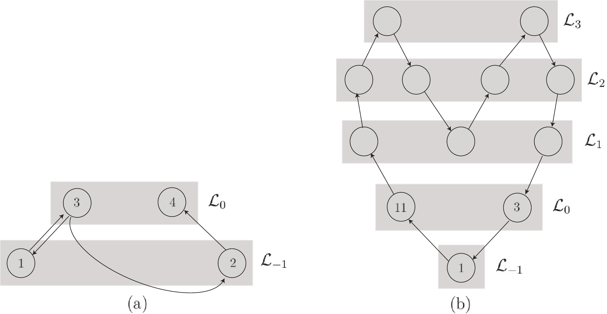
(a) ; (b) .
For a vertex and positive integers , , let denote the set of paths of length such that , for all and . Note that if and only if mod .
Lemma 2.2.
For any and all positive integers , with mod , we have
Proof.
Since each path in has no hold time, each element of may be viewed a path of the symmetric random walk on starting at the position which hits the origin at step for the first time. The reflection principle for the random walk gives
| (2.2) |
By Lemma 2.1, for each we have
| (2.3) |
Combining (2.2) and (2.3) we obtain the desired inequality.∎
2.3. Formulas for Birkhoff sums of the central Jacobian
Let and let be a path in the Markov diagram . The Birkhoff sum on the rectangle is a constant, which we denote by with a slight abuse of notation. From the structure of the Markov diagram described in Section 2.1, we derive two useful formulas for this constant.
- (i)
If , then
(2.4) - (ii)
If and then
(2.5)
2.4. Stopping time
We denote by the Lebesgue measure on , , . A rectangle (resp. block) is a product of two (resp. three) non-degenerate intervals in . For a rectangle we write
Similarly, for a block we write
For and , let denote the maximal rectangle containing on which is affine. Clearly for , for and for . An integer is a cutting time of if . We define a stopping time
| (2.6) |
Clearly we have if and only if is contained in the set
The stopping time is expressed as follows. Put for convenience.
Proposition 2.3.
For all we have
Before proceeding let us record two equalities. First,
| (2.7) |
The definition of the stopping time (2.6) implies
| (2.8) |
Proof of Proposition 2.3.
By (2.7) and (2.8) it suffices to consider the case . Clearly we have . We claim , for otherwise (2.5) implies , and there is such that and . From Lemma 2.4 below, it follows that is a cutting time of , a contradiction to the minimality in the definition of . This claim and (2.4) together imply for all with , and so the desired equality holds. ∎
Lemma 2.4.
Let and . Then is a cutting time of if and only if and .
Proof.
To show the ‘if’ part, suppose , and . Take with . Let denote the connected component of that contains . Then is a rectangle, is affine and . Hence is a cutting time of . To show the ‘only if’ part, let be a cutting time of . The definition of cutting time implies . Since , by (2.5) we obtain . ∎
2.5. Formula for the stopping time in terms of pullbacks
Let be a non-empty subset of and let . A connected component of is called a pullback of by . If is a pullback of by and is affine, we call an affine pullback of by , or simply an affine pullback. If is connected and is an affine pullback of by , then .
Proposition 2.5.
For any such that is finite and , we have
Proof.
In the case , we have and the desired equality is obvious. Suppose . Then holds. By Proposition 2.3, there exists such that . The pullback of the rectangle by that contains , denoted by , is an affine pullback and satisfies . Proposition 2.3 implies . In particular, is affine and . From the assumption , there exists an affine pullback of by satisfying and . Hence, does not exceed the minimum in the right-hand side of the desired equality in the proposition. The reverse inequality is obvious from the property of . ∎
2.6. Almost sure finiteness of the stopping time
Clearly, if then the set has positive Lebesgue measure. Otherwise this is a null set.
Proposition 2.6.
If then the stopping time is finite Lebesgue a.e. on .
Proof.
Proposition 2.3 and (2.4), (2.5) together imply for all . Recall (1.7) that converges almost surely to the positive constant . Hence, if then is finite Lebesgue a.e. on .
For the rest of the proof of Proposition 2.6 we assume . We need two lemmas.
Lemma 2.7.
For Lebesgue a.e. , there exists a pair of positive integers such that
Proof.
Put . Let be the increasing sequence of positive reals satisfying for all . For and , define
The central limit theorem applied to the sequence of independently identically distributed random variables with mean and variance yields
Choose a sequence of positive integers such that . By Borel-Cantelli’s lemma,
| (2.9) |
Define by
Lemma 2.8.
is finite Lebesgue a.e. on .
Proof.
By (2.7) and on , it suffices to show that is finite Lebesgue a.e. on . Recall that is a skew product over the piecewise affine fully branched map in (1.1) that preserves the Lebesgue measure on , and is constant on the sets , . By Lemma 2.7, for Lebesgue a.e. there exists a positive integer pair satisfying . Moreover, the definition of and the formulas (2.4), (2.5) together imply for all . Hence, Lebesgue a.e. point in is contained in the set
| (2.10) |
where , are positive integers and
It suffices to show that is a null set. For each we have
where denotes the floor function. Using Lemma 2.2 to bound and the identity for each path in , we have
for all sufficiently large . For the third inequality we have used Stirling’s formula for factorials to evaluate the binomial coefficient. This yields for all , , and therefore
as required. This completes the proof of Lemma 2.8. ∎
By virtue of (2.7), (2.8) and on , it suffices to show that is finite Lebesgue a.e. on . Let denote the set of positive even integers. If and is finite then . Put , and for . For each , is written as a finite union of pairwise disjoint rectangles with the properties that for some , , is affine and for some . Lemma 2.8 gives .
The map given by for has the skew product form
The map is a piecewise affine map on the interval with infinitely many full branches, leaving the normalized Lebesgue measure on the interval invariant and ergodic. From Birkhoff’s ergodic theorem for , is finite for Lebesgue a.e. . Moreover, (2.4) implies for . This together with Proposition 2.3 implies for Lebesgue a.e. . The proof of Proposition 2.6 is complete. ∎
2.7. An induced Markov map
For each let denote the collection of affine pullbacks of by which are contained in . We set
Elements of are pairwise disjoint, and the stopping time is constant on each element. We now define an induced map by on each , and put
Partition into , label the partition elements with an integer , and write and We have , and maps each affinely onto . Proposition 2.6 implies for .
2.8. Stopping time estimates
For put
Note that . Moreover we have , and the equality holds if and only if .
Proposition 2.9.
There exists such that for all and all we have
In particular, if then decays exponentially in .
To prove Proposition 2.9, we estimate the size of each element of the partition , and the cardinality of the set of elements with a given stopping time.
Lemma 2.10.
For all and all ,
Proof.

For each , define
Lemma 2.11.
For all we have
Proof.
For integers , , with and , let
If , then let
Note that if and only if mod . The reflection principle of the symmetric random walk on gives
| (2.11) |
2.9. Symbolic dynamics
For we put
Define coding maps and by
Note that and The coding maps are not injective. The next connection between the heterochaos baker maps and the Dyck system lies at the basis of the proof of Theorem C.
Theorem 2.12 ([32], Theorem 1.1).
For all we have
3. Mixing of all orders for the heterochaos baker maps
In this section we prove Theorem A. In Section 3.1 we show a certain invariance of correlations, which implies the sufficiency to consider only . In Section 3.2 we establish the exactness and -property of the corresponding maps, and in Section 3.3 complete the proof of Theorem A.
3.1. Invariance of correlations
Let be a probability space and let be a measurable map preserving . For an integer and functions , consider their correlations
where . It is well-known that is -mixing if and only if as for all .
Define an involution by
Proposition 3.1.
Let . For all , and integers with we have
3.2. Exactness and -property
Let be a probability space. For sub-sigma-algebras , of we write if for every there exists such that , where denotes the symmetric difference of sets. We write if and . If is a family of sub-sigma-algebras of , let denote the smallest sub-sigma-algebra that contains all the . If is a family of partitions of into measurable sets, let denote the smallest sub-sigma-algebra that contains all the .
Let be a measurable map preserving . For a sub-sigma-algebra of and , let . If has a measurable inverse, let . We say is exact if has no measurable inverse and . We say has -property if has a measurable inverse and there exists a sub-sigma-algebra of such that:
- (i)
.
- (ii)
.
- (iii)
.
If has -property, is usually called a Kolmogorov automorphism [33]. Exactness or -property implies mixing of all orders [26, Section 2.6].
Proposition 3.2.
For any , is exact and has -property.
For a proof of this proposition we need some notation and one preliminary lemma. For define by
Let denote the Borel sigma-algebra on a topological space .
Lemma 3.3.
If , then for any with positive Lebesgue measure and any , there exists such that .
Proof.
Since the collection of unions of countably many elements of is an algebra on , for any there exist finitely many elements of such that . If is sufficiently small, there exists such that , for otherwise we obtain the following contradiction: . ∎
Proof of Proposition 3.2.
Let satisfy . To verify the exactness of it suffices to show that . By Lemma 3.3, for any there exist and an affine pullback of of by such that . There exists such that , and therefore and
The last inequality is because is affine. Since is arbitrary we obtain .
Note that , has a measurable inverse, and the restriction is -invariant. Let denote the smallest sub-sigma-algebra of that contains . From the definition of the map (1.4) we obtain and . The argument in the previous paragraph shows . We have verified that has -property. ∎
Remark 3.4.
3.3. Proof of Theorem A
4. Exponential mixing for the heterochaos baker maps
In this section we prove Theorem B. In Section 4.1 we introduce towers with exponential tail associated with the heterochaos baker maps. In Section 4.2 we apply the results in [35] to the towers and use large deviations to complete the proof of Theorem B.
4.1. Towers
Put . We extend the stopping time to a function on in the obvious way, and still denote the extension by : for . We define a tower associated with by
For each , the -th floor is the set
We identify the ground floor with . Note that . Define a tower map by
Collapsing the -coordinate, we obtain the quotient tower and the tower map . The maps and , and are semiconjugated by the maps and respectively. Let denote the canonical projection. In summary, the following diagram commutes:
We fix a sigma-algebra on that is obtained by naturally transplanting the Borel sigma-algebra on . Each floor , is identified with , and so equipped with the restriction of the Lebesgue measure. If , then in view of Proposition 2.9 let denote the probability measure on given by
Since the Lebesgue measure on is -invariant, is -invariant. The measure is -invariant, and absolutely continuous with respect to the Lebesgue measure, and hence . The measure is -invariant.
4.2. Proof of Theorem B
Let . Let and let , . For a function on , let denote its lift to the tower associated with , i.e. . Note that .
The rest of the proof of Theorem B breaks into three steps, much in parallel to [35, Section 4.1] with one important difference in Step 2. In Step 1 we begin by approximating , , by functions , on which do not depend on the -coordinate. In Step 2 we provide error bounds of these approximations. Since [35, p.608 Sublemma] does not hold as a result of the breakdown of the condition (P4) (backward contraction) in [35], we estimate errors of these approximations using large deviations for the map in (1.1). In Step 3 we view , as functions on , and show exponential decay of their correlations by applying [35]. We then unify all these estimates.
Step 1: Approximations. Put for . Each floor , is partitioned into where is a copy of . Let denote the partition of into -components. It has the Markov property: For every , is the union of elements of . For we put . For , let denote the partition of which is obtained as the canonical projection of . For and , define by
Clearly is constant on each element of , and . Since does not depend on the -coordinate, we may view as a function on . Let . By the identities and , we have where
Step 2: Estimates of , . A direct calculation shows and a similar argument to the one in [35, p.608] shows Hence, upper bounds of , follow from the next lemma. For let denote the -Hölder norm of , namely
where denotes the Euclidean distance between and .
Lemma 4.1.
For any and any , there exist constants and such that for every ,
Proof.
Put
The minimal expansion rate by in the -direction is and the maximal contraction rate by in the -direction is . Since we have . Fix , and recall the definition of a block and the notation introduced in the beginning of Section 2.4. For each , is a block satisfying and Define
Put For every with , the Euclidean diameter of does not exceed . Since , this bound implies
| (4.1) |
For each let denote the element of that contains . Then is a rectangle satisfying , which implies
| (4.2) |
Recall that is a skew product over in (1.1) that preserves the Lebesgue measure on , and . From the large deviations applied to the sequence of independently identically distributed random variables , the sum in (4.2) decays exponentially in . There exist and such that
| (4.3) |
The first inequality is due to the -invariance of . Let denote the union of elements of . For any , either or holds. We have
| (4.4) |
Step3: Estimate of and an overall estimate. It is clear that the greatest common divisor of is . Using the Perron-Frobenius operator given by we write
We introduce a separation time by defining to be the smallest integer such that , lie in different elements of . For general points , , define if and otherwise. This defines a separation time . For define
For each define
Lemma 4.2.
For all and all , we have and .
Proof.
For each , has a measurable inverse, and the pullback of the measure by is absolutely continuous with respect to . The Radon-Nikodým derivative is constant on , which we denote by . Note that
Moreover, for all , and so From this and we obtain .
For all with we have If , then for each either or , , which implies Hence the conclusion of the lemma holds. ∎
By [35, Section 4.2] (see also [24, Theorem 1.5]), there exist and such that
Combining this with the estimates of , in Step 2, and then substituting , we obtain constants and such that
namely, the exponential mixing for . From this and Proposition 3.1 we obtain the exponential mixing for . Taking a pair of Hölder continuous functions on which are constant on sets , , we obtain the exponential mixing for and . The proof of Theorem B is complete. ∎
Remark 4.3.
In the case which is excluded in Theorem B, it is plausible that correlations for Hölder continuous functions decay only subexponentially. It would be nice to prove this. A close inspection into the counting argument in Section 2.2 and the stopping time estimate in Section 2.7 reveals , and as a result . It follows that the lift of the Lebesgue measure to the tower becomes an infinite measure, and the general result in [36] to draw subexponential decay of correlations is not applicable.
5. Exponential mixing for the Dyck system
In this last section we prove Theorem C. In Section 5.1, we identify the two ergodic measures of maximal entropy for the Dyck system. In Section 5.2 we show the invariance of correlations (modulo involution) under the replacement of the two measures. Section 5.3 provides two preliminary lemmas needed to transfer invariant measures on the two different spaces. In Section 5.4 we clarify a connection between one of the two ergodic measures of maximal entropy and the Lebesgue measure on . In Section 5.5 we complete the proof of Theorem C.
5.1. Measures of maximal entropy
Let be a Borel map acting on a topological space. For each -invariant Borel probability measure , let denote the measure-theoretic entropy of with respect to . If is finite, a measure which attains this supremum is called a measure of maximal entropy.
Following [20, Section 4], for each we define by
where the delta denotes Kronecker’s delta. These functions are used to indicate whether a bracket in a prescribed position in a sequence in is closed or not. Consider three shift invariant Borel sets
| (5.1) |
Any shift invariant ergodic measure on gives measure to one of these three sets (see [20, pp.102–103]).
Theorem 5.1 ([20], Section 4).
There exist two ergodic measures , of entropy which are Bernoulli and satisfy and . These two measures are precisely all the ergodic measures of maximal entropy for the two-sided Dyck shift.
Let (resp. ) denote the shift invariant measure on which is the push-forward of (resp. ) under the canonical projection . These two measures are precisely all the ergodic measures of maximal entropy for the one-sided Dyck shift.
We recall the result in [32] on measures of maximal entropy for the heterochaos baker maps. Let and .
Theorem 5.2 ([32], Theorem 1.2).
For any , there exist two -invariant ergodic Borel probability measures , of entropy which are Bernoulli, give positive weight to any non-empty open subset of , and satisfy
Moreover, if or then , are measures of maximal entropy for . If or then there is no ergodic measure of maximal entropy for other than , .
5.2. Invariance of correlations
We define an involution by and for , and by . Clearly is injective, and as in Lemma 5.4 below.
Proposition 5.3.
For all and all we have
Proof.
By Lemma 5.4 below, for any shift invariant measure on we have and where for . This implies . We have
and and . Hence the desired equality holds. ∎
Lemma 5.4.
We have , and .
Proof.
The second assertion of the lemma is a consequence of the first one, which was proved in [32, Section 3.5]. We include the proof here for the reader’s convenience. For and we set . It is enough to show that , namely . By the relations (1.5), either (i) , or (ii) for some and . In case (i), clearly we have . In case (ii), we have and , and so . ∎
5.3. Transferring invariant measures
In order to transfer invariant measures on the two different spaces under the coding map, we need two lemmas. We extend the central Jacobian to a function on in the obvious way, and still denote the extension by : for .
Lemma 5.5.
Let and let be an -invariant ergodic Borel probability measure satisfying .
- (a)
If then .
- (b)
If then .
- (c)
If then .
Proof.
Let
Note that is shift invariant and contains .
Lemma 5.6 ([32], Lemma 3.1).
For all , the restriction of to is a homeomorphism onto its image.
5.4. Connection to the Lebesgue measure
Since , and preserve the Lebesgue measure on .
Proposition 5.7.
We have , and
Proof.
Recall that the restriction of to is invertible, uniformly expanding in the -direction and uniformly contracting in the -direction. Using Proposition 2.6 to deal with the dynamics in the -direction, it is easy to see that
Moreover, is ergodic by Theorem A. Therefore, Shannon-McMillan-Breimann’s theorem yields
for Lebesgue a.e. where . Clearly we have
and hence . The reverse inequality is a consequence of Theorem 5.2. We have verified . By [32, Lemma 3.9] and we have .
5.5. Proof of Theorem C
First we show exponential mixing for , . To this end, by virtue of Proposition 5.3 it suffices to show that for any pair , of Hölder continuous functions on , their correlation decays exponentially in . This does not immediately follow from Theorem B. Indeed, Proposition 5.7 implies , but and may not be Hölder continuous. Our strategy is to transfer to the Dyck system the towers associated with , constructed in Section 4.1, and mimic the proof of Theorem B.
We restrict ourselves to the shift invariant set in (5.1). Bear in mind that . By Lemma 5.6, the restriction of to is a homeomorphism onto its image. We put
Define by . We define a tower
and define a tower map by
Collapsing the negative coordinate, we obtain the quotient tower and the tower map . We fix a sigma-algebra on that is obtained by naturally transplanting the Borel sigma-algebra on .
By Proposition 2.6, is finite -a.e. and . Each floor
can be identified with , and so equipped with the restriction of the measure . Let denote the probability measure on given by
We repeat Steps 1 to 3 in the proof of Theorem B in Section 3.3. Each floor is partitioned into where is a copy of . Let denote the partition of into -components. For , let . For and , define by for Define . For every , the diameter of the set with respect to the Hamming metric does not exceed . As a counterpart of (4.1) we have , where denotes the -Hölder norm of with respect to . Therefore, as a counterpart of Lemma 4.1 we obtain . To finish, the rest of the argument is completely analogous to Step 3 in the proof of Theorem B.
We have verified exponential mixing for both and . Taking a pair of Hölder continuous functions on which depend only on positive coordinates, we obtain exponential mixing for both and . The proof of Theorem C is complete. ∎
Acknowledgments
The author thanks Yoshitaka Saiki, Toshi Sugiyama, Masato Tsujii, Kenichiro Yamamoto, James A. Yorke for fruitful discussions. This research was supported by the JSPS KAKENHI 19K21835, 20H01811.
References
- [1] R. Abraham and S. Smale. Nongenericity of -stability. Global Analysis (Proc. Symp. Pure Math. Vol. XIV Berkley Calif., 1968) (1970) 5–8.
- [2] Alfred V. Aho and Jeffrey D. Ullman. The theory of languages, Math. Systems Theory 2 (1968) 97–125.
- [3] José F. Alves, Stefano Luzzatto and Vilton Pinheiro. Markov structures and decay of correlations for non-uniformly expanding dynamical systems. Ann. Inst. H. Poincaré Anal. Non Linéaire 22 (2005) 817–839.
- [4] Rafael A. Bilbao, Ricardo Bioni and Rafael Lucena. Hölder regularity and exponential decay of correlations for a class of piecewise partially hyperbolic maps. Nonlinearity 33 (2020) 6790–6818.
- [5] Jérôme Buzzi. Markov extensions for multi-dimensional dynamical systems. Israel J. Math. 112 (1999) 357–380.
- [6] Christian Bonatti and Lorenzo J. Díaz. Persistent nonhyperbolic transitive diffeomorphisms. Ann. of Math. 143 (1996) 357–396.
- [7] Rufus Bowen. Equilibrium states and the ergodic theory of Anosov diffeomorphisms, Second revised edition. Lecture Notes in Mathematics, 470 Springer-Verlag, Berlin 2008.
- [8] Augusto Armando de Castro Júnior. Backward inducing and exponential decay of correlations for partially hyperbolic attractors. Israel J. Math. 130 (2002) 29–75.
- [9] Augusto Armando de Castro Júnior. Fast mixing for attractors with a mostly contracting central direction. Ergodic Theory Dynam. Sys. 24 (2004) 17–44.
- [10] Armando Castro and Teófilo Nascimento. Statistical properties of the maximal entropy measure for partially hyperbolic attractors. Ergodic Theory Dynam. Systems 37 (2017) 1060–1101.
- [11] Vaughn Climenhaga. Specification and towers in shift spaces. Commun. Math. Phys. 364 (2018) 441–504.
- [12] Silvina Dawson, Celso Grebogi, Tim Sauer and James A. Yorke. Obstruction to shadowing when a Lyapunov exponent fluctuates about zero. Phys. Rev. Lett. 73 (1994) 1927.
- [13] Dmitry Dolgopyat. On dynamics of mostly contracting diffeomorphisms. Comm. Math. Phys. 213 (2000) 181–201.
- [14] Paul R. Halmos. Lectures on Ergodic Theory (Chelsea Publishing Company, New York, NY) 1956.
- [15] Franz Hofbauer. On intrinsic ergodicity of piecewise monotonic transformations with positive entropy I, II. Israel J. Math., 34 (1979) 213–237, 38 (1981) 107–115.
- [16] Franz Hofbauer. Piecewise invertible dynamical systems. Probability Theory and Related Fields. 72 (1986) 359–386.
- [17] Ale Jan Homburg and Charlene Kalle. Iterated function systems of affine expanding and contracting maps of the unit interval. arXiv:2207.09987
- [18] Gerhard Keller. Lifting measures to Markov extensions. Monatsh. Math. 108 (1989) 183–200.
- [19] Eric J. Kostelich, Ittai Kan, Celso Grebogi, Edward Ott and James A. Yorke. Unstable dimension variability: A source of nonhyperbolicity in chaotic systems. Phys. D 109 (1997) 81–90.
- [20] Wolfgang Krieger. On the uniqueness of the equilibrium state. Math. Systems Theory 8 (1974/75) 97–104.
- [21] Wolfgang Krieger. On a syntactically defined invariant of symbolic dynamics. Ergodic Theory Dynam. Systems 20 (2000) 501–516.
- [22] Ricardo Mañé. Contributions to the stability conjecture. Topology 17 (1978) 383–396.
- [23] Kengo Matsumoto. A simple purely infinite -algebra associated with a lambda-graph system of the Motzkin shift, Math. Z. 248 (2004) 369–394.
- [24] Véronique Maume-Deschamps. Projective metrics and mixing properties on towers. Trans. Amer. Math. Soc. 353 3371–3389 (2001)
- [25] Tom Meyerovitch. Tail invariant measures of the Dyck shift. Israel J. Math. 163 (2008) 61–83.
- [26] V. A. Rohlin. Exact endomorphisms of a Lebesgue space. Amer. Math. Soc. Transl. Ser.2 39 (1963) 1–36.
- [27] David Ruelle. Thermodynamic formalism. The mathematical structures of classical equilibrium statistical mechanics. Second edition. Cambridge University Press 2004.
- [28] Yoshitaka Saiki, Hiroki Takahasi and James A. Yorke. Piecewise linear maps with heterogeneous chaos. Nonlinearity 34 (2021) 5744–5761.
- [29] Yoshitaka Saiki, Hiroki Takahasi and James A. Yorke. Hausdorff dimension of Cantor intersections and robust heterodimensional cycles for heterochaos horseshoe maps. SIAM J. Appl. Dyn. Sys. to appear
- [30] Carl P. Simon. A -dimensional Abraham-Smale example. Proc. Amer. Math. Soc. 34 (1972) 629–630.
- [31] Ja. G. Sinaĭ. Gibbs measures in ergodic theory. Uspehi Mat. Nauk. 27 (1972) 21–64.
- [32] Hiroki Takahasi and Kenichiro Yamamoto. Heterochaos baker maps and the Dyck system: maximal entropy measures and a mechanism for the breakdown of entropy approachability. Proc. Amer. Math. Soc. https://doi.org/10.1090/proc/16538 arXiv:2209.04905
- [33] Peter Walters. An Introduction to Ergodic Theory. Graduate Texts in Mathematics 79, Springer-Verlag, New York, 1982.
- [34] Benjamin Weiss. Intrinsically ergodic systems. Bull. Amer. Math. Soc. 76 (1970) 1266–1269.
- [35] Lai Sang Young. Statistical properties of dynamical systems with some hyperbolicity. Ann. of Math. 147 (1998) 585–650.
- [36] Lai Sang Young. Recurrence times and rates of mixing. Israel J. Math. 110 (1999) 153–188.