The lightest supersymmetric (SUSY) partner of the top quark, the so-called top-squark $\tilde{t}_{1}$, has for long been a lucrative target for supersymmetry searches at hadron colliders. Early estimates of EENZ/BG[1, 2] naturalness, using the measure $\Delta_{BG}\equiv max_{i}|\frac{p_{i}}{m_{Z}^{2}}\frac{\partial m_{Z}^{2}}{\partial p_{i}}|<\Delta_{BG}(max)$ (where the $p_{i}$ are taken as fundamental theory parameters, usually assumed to be a set of high scale soft SUSY breaking terms) found $m_{\tilde{t}_{1}}\lesssim 300-400$ GeV for $\Delta_{BG}<10-30$[3]. Using an alternative measure $\delta m_{h}^{2}/m_{h}^{2}<\Delta_{HS}$, it was expected that three third generation squarks should all have mass $m_{\tilde{t}_{1,2},\tilde{b}_{1}}\lesssim 500$ GeV[4, 5, 6]. These theoretical naturalness computations may be compared to recent limits from LHC searches where both ATLAS[7, 8] and CMS[9] find that $m_{\tilde{t}_{1}}\gtrsim 1.2$ TeV from $pp$ collisions at $\sqrt{s}=13$ TeV and with $\sim 139$ fb^-1 of integrated luminosity. Taken at face value, this confrontation between theory and experiment would indicate that the paradigm of weak scale supersymmetry[10] is highly implausible as a route to physics beyond the Standard Model (SM)[11].

One resolution to the supersymmetry naturalness conflict is that the early theoretical naturalness calculations turned out to be large overestimates of the actual finetuning[12, 13]. For the BG measure, it is emphasized in Ref. [12, 14, 15, 13] that the fundamental theory parameters $p_{i}$ should not be taken as a set of independent soft SUSY breaking terms, since in any more UV-complete theory, these are all correlated. For example, in gravity-mediation SUSY breaking models with a well-specified SUSY breaking sector, then the soft terms are all computed as multiples of the gravitino mass $m_{3/2}$.¹¹ 1 For instance, in dilaton-dominated SUSY breaking, then $m_{0}=m_{3/2}$ with $A_{0}=-m_{1/2}=\sqrt{3}m_{3/2}$[16]. Adopting independent soft terms as the $p_{i}$ just parametrizes our ignorance of the SUSY breaking mechanism, but can lead to overestimates of finetuning by up to three orders of magnitude[13]. Alternatively, the $\Delta_{HS}$ measure attempts to tune dependent quantities $m_{H_{u}}^{2}$ and $\delta m_{H_{u}}^{2}$ one against the other, which again leads to up to three orders of magnitude overestimates of finetuning[13]. If one instead adopts the more conservative electroweak finetuning measure $\Delta_{EW}$[17, 18], then top-squark masses are allowed up to several TeV at little cost to finetuning since their contributions to the weak scale are suppressed by loop factors (for a recent review, see e.g. Ref. [19]).

In most supersymmetric models of particle physics– even in the case of high scale scalar mass universality– the lighter top squark $\tilde{t}_{1}$ is expected to be the lightest of all the squarks. It thus presents a lucrative target for supersymmetry discovery at hadron collider experiments such as the CERN LHC. The lightness of the top squark, relative to other squarks, arises from two reasons: 1. the large top-quark Yukawa coupling $f_{t}$ acts to drive top squark soft terms to lower values than other squarks (assuming an initial degeneracy amongst all squark soft terms at the high scale) and 2. the large top Yukawa enhances the mixings amongst the top squarks, and large mixing typically acts to further split the top squark eigenmasses, driving the lighter one down and the heavier stop $\tilde{t}_{2}$ to larger values (relative to the no mixing case).

A third effect arises from the string landscape picture[20, 21, 22]. In the string landscape, where of order $10^{500}$ vacua solutions[23] arise from compactification from 10 to 4 spacetime dimensions, then each vacuum solution corresponds to a different set of $4-d$ low energy effective field theory law of physics. The string landscape provides a natural setting for Weinberg’s anthropic solution to the cosmological constant problem[24] in an eternally inflating multiverse. If similar reasoning is applied to the origin of the SUSY breaking scale, then it is expected that no particular value of the (complex-valued) SUSY breaking $F$ terms or (real-valued) SUSY breaking $D$-terms are favored over any other. In that case, then on rather general grounds, the landscape is expected to statistically favor large soft terms via a power law[25]

where $f_{SUSY}$ encodes the expected statistical distribution of landscape soft terms. Thus, even the textbook case of SUSY breaking via a single $F$-term field would yield a linear draw to large soft terms.

Naively, one might expect such a distribution to favor high scale SUSY breaking. However, the weak scale soft terms and SUSY-preserving $\mu$ parameter determine the magnitude of the weak scale via the scalar potential minimization conditions under the radiative breaking of electroweak symmetry:

where the label $PU$ stands for parameter values in each separate pocket universe within the greater multiverse. Here, following Weinberg, we assume a so-called fertile patch of the multiverse wherein the low energy/weak scale effective field theory (LE-EFT) consists of the MSSM (plus some additional fields such as a PQ sector) but with variable soft terms and hence variable values for the associated weak scale $m_{weak}^{PU}$. The value of $m_{weak}^{PU}$ is typically $\neq m_{weak}^{OU}$, where $OU$ stands for a quantity’s value in our universe. Agrawal et al. (ABDS)[26] have shown that for complex nuclei– and hence atoms as we know them– to form in a PU, that the value of $m_{weak}^{PU}$ must lie within the ABDS window, typically $m_{weak}^{PU}\sim(0.5-5)m_{weak}^{OU}$ (the atomic principle). The ABDS anthropic window thus vetoes vacua with improper electroweak symmetry breaking (EWSB), such as solutions with no EWSB or charge or color breaking (CCB) minima; it also excludes the vast majority of high scale SUSY solutions which typically lead to $m_{weak}^{PU}$ far beyond the ABDS window. The string landscape approach to soft SUSY breaking within the MSSM has led to some success in that it statistically predicts a Higgs boson mass $m_{h}\simeq 125$ GeV whilst sparticles are typically well beyond current LHC search bounds[27].

Returning to top squarks, the large value of the top quark Yukawa coupling enhances the radiative correction terms $\Sigma_{u}^{u}(\tilde{t}_{1,2})$ in Eq. 2 relative to $\Sigma_{u}^{u}(\tilde{q}_{i})$ (where $\tilde{q}_{i}$ denotes squark masses of the first two generations. Thus, for independent soft terms for each generation (as is generic in gravity mediation[28, 29, 16]) then the squark and slepton masses of the first two generations will get pulled to much higher values, typically $m_{\tilde{q}_{i}}\sim 10-40$ TeV (providing a mixed decoupling/quasi-degeneracy solution to the SUSY flavor and CP problems[30]) whilst $m_{\tilde{t}_{1}}\sim 1-2.5$ TeV. As such, the string landscape provides additional strong motivation for top-squark pair searches at LHC as compared to other sparticle searches (although the search for light higgsinos with $m(higgsino)\sim 100-400$ GeV is also especially lucrative[31, 32, 33, 34, 35, 36]).

In this paper, after a brief review of some previous relevant works in Subsec. 1.1, in Sec. 2 we will present landscape predictions for some of the relevant properties of light top squarks as derived from string landscape predictions with a simple $n=1$ power law draw to large soft terms. We will find that while large stop mixing terms $m_{t}A_{t}$ are expected at the weak scale (and indeed these help boost up the light Higgs mass to $m_{h}\sim 125$ GeV), the lighter top squark $\tilde{t}_{1}$ is still typically mainly a right-top-squark (assuming high scale degeneracy of left and right top squark soft terms $m_{\tilde{t}_{L}}$ and $m_{\tilde{t}_{R}}$, as expected by intragenerational degeneracy since the elements of each generation fill out the 16-dimensional spinor-rep of $SO(10)$). Also, we will find that the branching fraction $BR(b\rightarrow s\gamma)$ is expected to be very near its Standard Model (SM) value (in agreement with data and in accord with the general expectation for TeV-scale top-squarks). We will also determine the expected $\tilde{t}_{1}$ branching fractions which will determine the associated LHC search signatures. In Sec. 3, we examine top-squark pair production rates and expected signal channels which are expected for HL-LHC searches. In Sec. 4 we introduce a natural top-squark benchmark point and associated model line. In Sec. 5, we give cuts and $m_{T_{2}}$ distributions for each of the the three major signal channels. By combining results, we present $5\sigma$ reach and 95%CL exclusion limits versus $m_{\tilde{t}_{1}}$. In Sec. 6, we present a brief summary and conclusions from our results.

For the benefit of the reader, we show in Fig. 8 the next-to-leading-order (NLO) Prospino[65] prediction for top squark pair production at LHC with $\sqrt{s}=14$ TeV collisions: $\sigma(pp\rightarrow\tilde{t}_{1}\tilde{t}_{1}^{*}X)$ vs. $m_{\tilde{t}_{1}}$. Starting just above the present LHC excluded region, with $m_{\tilde{t}_{1}}=1.25$ TeV, we find $\sigma(\tilde{t}_{1}\tilde{t}_{1}^{*})\sim 1$ fb, corresponding to 3000 signal events assuming the nominal HL-LHC integrated luminosity of 3 ab^-1. Even for $m_{\tilde{t}_{1}}$ as high as 2 TeV, we find $\sigma(\tilde{t}_{1}\tilde{t}_{1}^{*})\sim 0.02$ fb, corresponding to 60 signal events at HL-LHC before cuts.

The projected HL-LHC reach for top squark pair producton is usually presented in terms of simplified models by the ATLAS and CMS collaborations where a single top squark decay mode is assumed. We see from the previous subsection that such analyses are not realistic from the point of view of the string landscape and so we will examine the reach of LHC at HL-LHC using the several predicted decay modes. This will give rise to mixed decay mode configurations such as is shown in Fig. 9 where one $\tilde{t}_{1}\rightarrow b\tilde{\chi}_{1}^{+}$ and the other $\tilde{t}_{1}\rightarrow t\tilde{\chi}_{1}^{0}$. Thus, we expect three main signal channels:

• •

  $b\bar{b}+\not\!\!\!{E_{T}}$,

• •

  $t\bar{t}+\not\!\!\!{E_{T}}$ and

• •

  $t\bar{b}+\not\!\!\!{E_{T}}$ (plus charge conjugate mode).

In addition, some subset of events will contain soft decay products from the unstable higgsinos in the cascade decay. Of particular note is the ocassional presence of $\tilde{\chi}_{2}^{0}\rightarrow\tilde{\chi}_{1}^{0}\ell\bar{\ell}$ (with $\ell=e$ or $\mu$) where $m(\ell\bar{\ell})<m_{\tilde{\chi}_{2}^{0}}-m_{\tilde{\chi}_{1}^{0}}$.

In the following Section, we will examine top squark pair production at LHC14 for the following Benchmark Point (BM) which is typical of stringy natural models. The BM point comes from the NUHM2 model[52] with parameters as listed in the Table 1. It is a natural SUSY benchmark point since $\Delta_{EW}=22$, even though the lightest top squark lies at $m_{\tilde{t}_{1}}\sim 1.7$ TeV and $m_{\tilde{g}}\sim 2.8$ TeV. The spectra is generated using the Isasugra code[66] from Isajet[54]. We can also expand this natural SUSY BM point into a natural SUSY Model Line by simply varying the $A_{0}$ parameter which results in variation of $m_{\tilde{t}_{1}}:800-2200$ GeV while hardly changing $m_{h}$ or other sparticle masses.

We next examine the reach of HL-LHC ($\sqrt{s}=14$ TeV with 3000 fb^-1) for the top squarks of stringy natural SUSY. To proceed, we generate a SUSY Les Houches Accord (SLHA) file[67] for our natural SUSY BM point and feed this into Pythia[68] which is used for signal and the $2\rightarrow 2$ background (BG) processes. For the $2\rightarrow 3$ BG processes, we use Madgraph[69] coupled to Pythia. The SM BGs considered are: $t\bar{t}$, $b\bar{b}Z$, $t\bar{t}Z$, $t\bar{t}W$, $b\bar{b}W$ and single-top production. We adopt the toy detector simulation Delphes[70].

The baseline reconstructed objects are as follows.

Baseline small radius(SR) jet:

1. 1.

   Found by anti-$k_{t}$ jet finder algorithm with $p_{T}(min)=25$ GeV and $R=0.4$ and

2. 2.

   $|\eta(j)|<4.5$.

Isolated lepton:

1. 1.

   $|\eta(\mu)|<2.5$ for muon, $|\eta(e)|<2.47$ for electron,

2. 2.

   $p_{T}(\mu)>25$ GeV for muon, $p_{T}(e)>20$ GeV for electron.

Large radius(LR) jet:

1. 1.

   Found by Cambridge/Aachen finder algorithm with $p_{T}(min)=400$ GeV with $R=1.5$.

For signal objects, we also require signal b-jets:

1. 1.

   satisfy the baseline SR jet requirement above.

2. 2.

   $|\eta(b)|<2.4$ and

3. 3.

   tagged by Delphes as $b$-jet.

The signal top candidate is reconstructed with either of the following criteria:

• •

  The fat jet $J$ is tagged by the HEPTopTagger2[71, 72] as a top. In such case, the top 4-vector reconstructed by the tagger is used for further kinematics calculations, or

• •

  The fat jet $J$ has a trimmed mass $115\ {\rm GeV}<m_{J}<225$ GeV and has at least 1 $b$-jet within the cone radius of the fat jet $(\Delta R(J,b)<1.5$). In such a case, the trimmed 4-vector of the fat jet is used for further kinematics calculations.

The events then are separated into three channels: $t\bar{t}+\not\!\!\!{E_{T}}$, $tb+\not\!\!\!{E_{T}}$, and $b\bar{b}+\not\!\!\!{E_{T}}$. The workflow to determine each channel is as follows:

• •

  If there are at least 2 tops being tagged by the HEPTopTagger2, the two tops with the hardest $p_{T}$ are chosen as signals, and this channel is labeled as $t\bar{t}+\not\!\!\!{E_{T}}$.

• •

  Otherwise, if the HEPTopTagger2 tags 1 top, and the trimming method tags at least one other, this channel is labeled again as $t\bar{t}+\not\!\!\!{E_{T}}$. The top tagged by the HEPTopTagger2, and the hardest fat jet found by the trimming method are chosen as signals.

• •

  Otherwise, if the HEPTopTagger2 fails to tag any tops, but the trimming method found at least two, this channel is also labeled as $t\bar{t}+\not\!\!\!{E_{T}}$. The two tops with the hardest $p_{T}$ are chosen as signals.

• •

  Otherwise, if there is exactly 1 top tagged by either HEPTopTagger2 or the trimming method, then look for extra $b$-jet candidates. The $b$-jet candidates must satisfy signal $b$-jet requirement listed above. The $b$-jet candidate needs to be well separated with the 3 subjets of the reconstructed top (Both HEPTopTagger2 and the trimming algorithm can provide the subjet 4-vectors): $\Delta R(subjet,b)>0.4$. If there are $b$-jets satisfying these requirements, the $b$ candidate that minimizes the vector sum of $\not\!\!\!{E_{T}}+p_{T}(t)+p_{T}(b)$ is chosen as the signal. This channel is labeled as $tb+\not\!\!\!{E_{T}}$.

• •

  Otherwise, if the event fails any of the above selection requirements but has at least two $b$ jets satisfied the signal $b$-jet requirement, this channel is labeled as $b\bar{b}+\not\!\!\!{E_{T}}$. The pair of $b$-jets that minimize the vector sum of $\not\!\!\!{E_{T}}+p_{T}(b_{1})+p_{T}(b_{2})$ are chosen as signals. The harder of the two is labeled as $b_{1}$, and the other is $b_{2}$ in the following.

In this paper we have examined what sort of values of top squark masses and other properties are expected from the string landscape where a power-law draw to large soft terms is expected, but where the derived value of the weak scale must lie within the ABDS window in order to allow for complex nuclei (and hence atoms) in each anthropically-allowed pocket universe. Under this stringy naturalness requirement, we find $m_{\tilde{t}_{1}}\sim 1-2.5$ TeV with large mixing. These results are in accord with measurements of $BR(b\rightarrow s\gamma)$ which are suggestive of TeV-scale top-squarks so that SUSY contributions to this decay rate decouple. The large mixing helps boost $m_{h}\rightarrow 125$ GeV while minimizing the top squark contributions to the weak scale $\Sigma_{u}^{u}(\tilde{t}_{1,2})$.

In spite of the large mixing, the lighter top-squark is mainly a right-squark, but decays at $\tilde{t}_{1}\rightarrow b\tilde{\chi}_{1}^{+}$ at $\sim 50\%$ and $\tilde{t}_{1}\rightarrow t\tilde{\chi}_{1,2}^{0}$ at $\sim 25\%$ each. Thus, we expect top-squark pair production at LHC Run 3 and HL-LHC to lead to mixed final states of $b\bar{b}+\not\!\!\!{E_{T}}$, $t\bar{t}+\not\!\!\!{E_{T}}$ and $tb+\not\!\!\!{E_{T}}$. We evaluated some optimized cuts for each of these channels, and then expect the top-squark pair production to be revealed as an enhancement in the $m_{T_{2}}$ distribution at high values of $m_{T_{2}}$. We combined the reaches in these three channels to find that HL-LHC operating at $\sqrt{s}=14$ TeV with 3000 fb^-1 of integrated luminosity should have a $5\sigma$ discovery reach to $m_{\tilde{t}_{1}}\sim 1.7$ TeV and a 95% CL exclusion reach to about $m_{\tilde{t}_{1}}\sim 2$ TeV. Now our HL-LHC reach results can be added to Fig. 1b) as a final summary frame: Fig. 14.

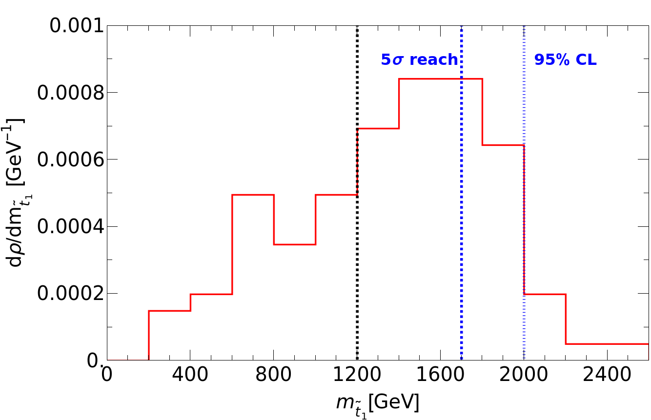
These HL-LHC reach limits will cover most (but not all) of the expected stringy natural parameter space from SUSY on the landscape!

Acknowledgements:

This material is based upon work supported by the U.S. Department of Energy, Office of Science, Office of High Energy Physics under Award Number DE-SC-0009956 and DE-SC-0017647.

References

- [1] J. R. Ellis, K. Enqvist, D. V. Nanopoulos, F. Zwirner, Observables in Low-Energy Superstring Models, Mod. Phys. Lett. A 1 (1986) 57. doi:10.1142/S0217732386000105.
- [2] R. Barbieri, G. F. Giudice, Upper Bounds on Supersymmetric Particle Masses, Nucl. Phys. B 306 (1988) 63–76. doi:10.1016/0550-3213(88)90171-X.
- [3] S. Dimopoulos, G. F. Giudice, Naturalness constraints in supersymmetric theories with nonuniversal soft terms, Phys. Lett. B 357 (1995) 573–578. arXiv:hep-ph/9507282, doi:10.1016/0370-2693(95)00961-J.
- [4] R. Kitano, Y. Nomura, Supersymmetry, naturalness, and signatures at the LHC, Phys. Rev. D 73 (2006) 095004. arXiv:hep-ph/0602096, doi:10.1103/PhysRevD.73.095004.
- [5] M. Papucci, J. T. Ruderman, A. Weiler, Natural SUSY Endures, JHEP 09 (2012) 035. arXiv:1110.6926, doi:10.1007/JHEP09(2012)035.
- [6] C. Brust, A. Katz, S. Lawrence, R. Sundrum, SUSY, the Third Generation and the LHC, JHEP 03 (2012) 103. arXiv:1110.6670, doi:10.1007/JHEP03(2012)103.
- [7] G. Aad, et al., Search for a scalar partner of the top quark in the all-hadronic plus missing transverse momentum final state at TeV with the ATLAS detector, Eur. Phys. J. C 80 (8) (2020) 737. arXiv:2004.14060, doi:10.1140/epjc/s10052-020-8102-8.
- [8] G. Aad, et al., Search for new phenomena with top quark pairs in final states with one lepton, jets, and missing transverse momentum in collisions at = 13 TeV with the ATLAS detector, JHEP 04 (2021) 174. arXiv:2012.03799, doi:10.1007/JHEP04(2021)174.
- [9] A. M. Sirunyan, et al., Search for top squark production in fully-hadronic final states in proton-proton collisions at 13 TeV, Phys. Rev. D 104 (5) (2021) 052001. arXiv:2103.01290, doi:10.1103/PhysRevD.104.052001.
- [10] H. Baer, X. Tata, Weak scale supersymmetry: From superfields to scattering events, Cambridge University Press, 2006.
- [11] M. Dine, Naturalness Under Stress, Ann. Rev. Nucl. Part. Sci. 65 (2015) 43–62. arXiv:1501.01035, doi:10.1146/annurev-nucl-102014-022053.
- [12] H. Baer, V. Barger, D. Mickelson, How conventional measures overestimate electroweak fine-tuning in supersymmetric theory, Phys. Rev. D 88 (9) (2013) 095013. arXiv:1309.2984, doi:10.1103/PhysRevD.88.095013.
- [13] H. Baer, V. Barger, D. Martinez, S. Salam, On practical naturalness and its implications for weak scale supersymmetryarXiv:2305.16125.
- [14] A. Mustafayev, X. Tata, Supersymmetry, Naturalness, and Light Higgsinos, Indian J. Phys. 88 (2014) 991–1004. arXiv:1404.1386, doi:10.1007/s12648-014-0504-8.
- [15] H. Baer, V. Barger, D. Mickelson, M. Padeffke-Kirkland, SUSY models under siege: LHC constraints and electroweak fine-tuning, Phys. Rev. D 89 (11) (2014) 115019. arXiv:1404.2277, doi:10.1103/PhysRevD.89.115019.
- [16] A. Brignole, L. E. Ibanez, C. Munoz, Towards a theory of soft terms for the supersymmetric Standard Model, Nucl. Phys. B 422 (1994) 125–171, [Erratum: Nucl.Phys.B 436, 747–748 (1995)]. arXiv:hep-ph/9308271, doi:10.1016/0550-3213(94)00068-9.
- [17] H. Baer, V. Barger, P. Huang, A. Mustafayev, X. Tata, Radiative natural SUSY with a 125 GeV Higgs boson, Phys. Rev. Lett. 109 (2012) 161802. arXiv:1207.3343, doi:10.1103/PhysRevLett.109.161802.
- [18] H. Baer, V. Barger, P. Huang, D. Mickelson, A. Mustafayev, X. Tata, Radiative natural supersymmetry: Reconciling electroweak fine-tuning and the Higgs boson mass, Phys. Rev. D 87 (11) (2013) 115028. arXiv:1212.2655, doi:10.1103/PhysRevD.87.115028.
- [19] H. Baer, V. Barger, S. Salam, D. Sengupta, K. Sinha, Status of weak scale supersymmetry after LHC Run 2 and ton-scale noble liquid WIMP searches, Eur. Phys. J. ST 229 (21) (2020) 3085–3141. arXiv:2002.03013, doi:10.1140/epjst/e2020-000020-x.
- [20] R. Bousso, J. Polchinski, The string theory landscape, Sci. Am. 291 (2004) 60–69. doi:10.1038/scientificamerican0904-78.
- [21] L. Susskind, The Anthropic landscape of string theory (2003) 247–266arXiv:hep-th/0302219.
- [22] M. R. Douglas, S. Kachru, Flux compactification, Rev. Mod. Phys. 79 (2007) 733–796. arXiv:hep-th/0610102, doi:10.1103/RevModPhys.79.733.
- [23] S. Ashok, M. R. Douglas, Counting flux vacua, JHEP 01 (2004) 060. arXiv:hep-th/0307049, doi:10.1088/1126-6708/2004/01/060.
- [24] S. Weinberg, Anthropic Bound on the Cosmological Constant, Phys. Rev. Lett. 59 (1987) 2607. doi:10.1103/PhysRevLett.59.2607.
- [25] M. R. Douglas, Statistical analysis of the supersymmetry breaking scalearXiv:hep-th/0405279.
- [26] V. Agrawal, S. M. Barr, J. F. Donoghue, D. Seckel, Viable range of the mass scale of the standard model, Phys. Rev. D 57 (1998) 5480–5492. arXiv:hep-ph/9707380, doi:10.1103/PhysRevD.57.5480.
- [27] H. Baer, V. Barger, H. Serce, K. Sinha, Higgs and superparticle mass predictions from the landscape, JHEP 03 (2018) 002. arXiv:1712.01399, doi:10.1007/JHEP03(2018)002.
- [28] S. K. Soni, H. A. Weldon, Analysis of the Supersymmetry Breaking Induced by N=1 Supergravity Theories, Phys. Lett. B 126 (1983) 215–219. doi:10.1016/0370-2693(83)90593-2.
- [29] V. S. Kaplunovsky, J. Louis, Model independent analysis of soft terms in effective supergravity and in string theory, Phys. Lett. B 306 (1993) 269–275. arXiv:hep-th/9303040, doi:10.1016/0370-2693(93)90078-V.
- [30] H. Baer, V. Barger, D. Sengupta, Landscape solution to the SUSY flavor and CP problems, Phys. Rev. Res. 1 (3) (2019) 033179. arXiv:1910.00090, doi:10.1103/PhysRevResearch.1.033179.
- [31] H. Baer, V. Barger, P. Huang, Hidden SUSY at the LHC: the light higgsino-world scenario and the role of a lepton collider, JHEP 11 (2011) 031. arXiv:1107.5581, doi:10.1007/JHEP11(2011)031.
- [32] Z. Han, G. D. Kribs, A. Martin, A. Menon, Hunting quasidegenerate Higgsinos, Phys. Rev. D 89 (7) (2014) 075007. arXiv:1401.1235, doi:10.1103/PhysRevD.89.075007.
- [33] H. Baer, A. Mustafayev, X. Tata, Monojet plus soft dilepton signal from light higgsino pair production at LHC14, Phys. Rev. D 90 (11) (2014) 115007. arXiv:1409.7058, doi:10.1103/PhysRevD.90.115007.
- [34] C. Han, D. Kim, S. Munir, M. Park, Accessing the core of naturalness, nearly degenerate higgsinos, at the LHC, JHEP 04 (2015) 132. arXiv:1502.03734, doi:10.1007/JHEP04(2015)132.
- [35] H. Baer, V. Barger, S. Salam, D. Sengupta, X. Tata, The LHC higgsino discovery plane for present and future SUSY searches, Phys. Lett. B 810 (2020) 135777. arXiv:2007.09252, doi:10.1016/j.physletb.2020.135777.
- [36] H. Baer, V. Barger, D. Sengupta, X. Tata, New angular and other cuts to improve the Higgsino signal at the LHC, Phys. Rev. D 105 (9) (2022) 095017. arXiv:2109.14030, doi:10.1103/PhysRevD.105.095017.
- [37] I. I. Y. Bigi, S. Rudaz, SEARCH FOR SCALAR SUPERPARTNERS OF THE TOP QUARK, Phys. Lett. B 153 (1985) 335–340. doi:10.1016/0370-2693(85)90560-X.
- [38] H. Baer, X. Tata, Implications of the T Quark Signal for Stop Squarks and Charged Higgs Bosons, Phys. Lett. B 167 (1986) 241–247. doi:10.1016/0370-2693(86)90607-6.
- [39] H. Baer, M. Drees, R. Godbole, J. F. Gunion, X. Tata, Phenomenology of light top squarks at the Fermilab Tevatron, Phys. Rev. D 44 (1991) 725–740. doi:10.1103/PhysRevD.44.725.
- [40] H. Baer, J. Sender, X. Tata, The Search for top squarks at the Fermilab Tevatron Collider, Phys. Rev. D 50 (1994) 4517–4528. arXiv:hep-ph/9404342, doi:10.1103/PhysRevD.50.4517.
- [41] K. Rolbiecki, J. Tattersall, G. Moortgat-Pick, Towards Measuring the Stop Mixing Angle at the LHC, Eur. Phys. J. C 71 (2011) 1517. arXiv:0909.3196, doi:10.1140/epjc/s10052-010-1517-x.
- [42] F. Brummer, S. Kraml, S. Kulkarni, Anatomy of maximal stop mixing in the MSSM, JHEP 08 (2012) 089. arXiv:1204.5977, doi:10.1007/JHEP08(2012)089.
- [43] M. L. Graesser, J. Shelton, Hunting Mixed Top Squark Decays, Phys. Rev. Lett. 111 (12) (2013) 121802. arXiv:1212.4495, doi:10.1103/PhysRevLett.111.121802.
- [44] H. Baer, V. Barger, N. Nagata, M. Savoy, Phenomenological profile of top squarks from natural supersymmetry at the LHC, Phys. Rev. D 95 (5) (2017) 055012, [Addendum: Phys.Rev.D 103, 059902 (2021)]. arXiv:1611.08511, doi:10.1103/PhysRevD.95.055012.
- [45] C. Han, J. Ren, L. Wu, J. M. Yang, M. Zhang, Top-squark in natural SUSY under current LHC run-2 data, Eur. Phys. J. C 77 (2) (2017) 93. arXiv:1609.02361, doi:10.1140/epjc/s10052-017-4662-7.
- [46] Y. Bai, J. Berger, J. Osborne, B. A. Stefanek, Search for Heavy Stops with Merged Top-Jets, Phys. Rev. D 96 (9) (2017) 095035. arXiv:1611.05046, doi:10.1103/PhysRevD.96.095035.
- [47] ATLAS sensitivity to top squark pair production at the HL-LHC, ATL-PHYS-PUB-2018-021 (2018).
- [48] X. Cid Vidal, et al., Report from Working Group 3: Beyond the Standard Model physics at the HL-LHC and HE-LHC, CERN Yellow Rep. Monogr. 7 (2019) 585–865. arXiv:1812.07831, doi:10.23731/CYRM-2019-007.585.
- [49] H. Baer, V. Barger, S. Salam, D. Sengupta, String landscape guide to soft SUSY breaking terms, Phys. Rev. D 102 (7) (2020) 075012. arXiv:2005.13577, doi:10.1103/PhysRevD.102.075012.
- [50] M. R. Douglas, The String landscape and low energy supersymmetry, 2012, pp. 261–288. arXiv:1204.6626, doi:10.1142/9789814412551_0012.
- [51] H. Baer, V. Barger, S. Salam, Naturalness versus stringy naturalness (with implications for collider and dark matter searches), Phys. Rev. Research. 1 (2019) 023001. arXiv:1906.07741, doi:10.1103/PhysRevResearch.1.023001.
- [52] H. Baer, A. Mustafayev, S. Profumo, A. Belyaev, X. Tata, Direct, indirect and collider detection of neutralino dark matter in SUSY models with non-universal Higgs masses, JHEP 07 (2005) 065. arXiv:hep-ph/0504001, doi:10.1088/1126-6708/2005/07/065.
- [53] K. J. Bae, H. Baer, V. Barger, D. Sengupta, Revisiting the SUSY problem and its solutions in the LHC era, Phys. Rev. D 99 (11) (2019) 115027. arXiv:1902.10748, doi:10.1103/PhysRevD.99.115027.
- [54] F. E. Paige, S. D. Protopopescu, H. Baer, X. Tata, ISAJET 7.69: A Monte Carlo event generator for pp, anti-p p, and e+e- reactionsarXiv:hep-ph/0312045.
- [55] M. Carena, H. E. Haber, Higgs Boson Theory and Phenomenology, Prog. Part. Nucl. Phys. 50 (2003) 63–152. arXiv:hep-ph/0208209, doi:10.1016/S0146-6410(02)00177-1.
- [56] H. Baer, V. Barger, A. Mustafayev, Implications of a 125 GeV Higgs scalar for LHC SUSY and neutralino dark matter searches, Phys. Rev. D 85 (2012) 075010. arXiv:1112.3017, doi:10.1103/PhysRevD.85.075010.
- [57] V. Barger, P. Huang, M. Ishida, W.-Y. Keung, Scalar-Top Masses from SUSY Loops with 125 GeV mh and Precise Mw, Phys. Lett. B 718 (2013) 1024–1030. arXiv:1206.1777, doi:10.1016/j.physletb.2012.11.049.
- [58] V. D. Barger, J. L. Hewett, R. J. N. Phillips, New Constraints on the Charged Higgs Sector in Two Higgs Doublet Models, Phys. Rev. D 41 (1990) 3421–3441. doi:10.1103/PhysRevD.41.3421.
- [59] H. Baer, M. Brhlik, QCD improved b — s gamma constraints on the minimal supergravity model, Phys. Rev. D 55 (1997) 3201–3208. arXiv:hep-ph/9610224, doi:10.1103/PhysRevD.55.3201.
- [60] H. Baer, M. Brhlik, D. Castano, X. Tata, b — s gamma constraints on the minimal supergravity model with large tan Beta, Phys. Rev. D 58 (1998) 015007. arXiv:hep-ph/9712305, doi:10.1103/PhysRevD.58.015007.
- [61] M. Misiak, Radiative Decays of the Meson: a Progress Report, Acta Phys. Polon. B 49 (2018) 1291–1300. doi:10.5506/APhysPolB.49.1291.
- [62] Y. Amhis, et al., Averages of -hadron, -hadron, and -lepton properties as of 2021arXiv:2206.07501.
- [63] A. Limosani, et al., Measurement of Inclusive Radiative B-meson Decays with a Photon Energy Threshold of 1.7-GeV, Phys. Rev. Lett. 103 (2009) 241801. arXiv:0907.1384, doi:10.1103/PhysRevLett.103.241801.
- [64] J. P. Lees, et al., Precision Measurement of the Photon Energy Spectrum, Branching Fraction, and Direct CP Asymmetry , Phys. Rev. Lett. 109 (2012) 191801. arXiv:1207.2690, doi:10.1103/PhysRevLett.109.191801.
- [65] W. Beenakker, R. Hopker, M. Spira, PROSPINO: A Program for the production of supersymmetric particles in next-to-leading order QCDarXiv:hep-ph/9611232.
- [66] H. Baer, C.-H. Chen, R. B. Munroe, F. E. Paige, X. Tata, Multichannel search for minimal supergravity at and colliders, Phys. Rev. D 51 (1995) 1046–1050. arXiv:hep-ph/9408265, doi:10.1103/PhysRevD.51.1046.
- [67] P. Z. Skands, et al., SUSY Les Houches accord: Interfacing SUSY spectrum calculators, decay packages, and event generators, JHEP 07 (2004) 036. arXiv:hep-ph/0311123, doi:10.1088/1126-6708/2004/07/036.
- [68] T. Sjostrand, S. Mrenna, P. Z. Skands, PYTHIA 6.4 Physics and Manual, JHEP 05 (2006) 026. arXiv:hep-ph/0603175, doi:10.1088/1126-6708/2006/05/026.
- [69] J. Alwall, M. Herquet, F. Maltoni, O. Mattelaer, T. Stelzer, MadGraph 5 : Going Beyond, JHEP 06 (2011) 128. arXiv:1106.0522, doi:10.1007/JHEP06(2011)128.
- [70] J. de Favereau, C. Delaere, P. Demin, A. Giammanco, V. Lemaître, A. Mertens, M. Selvaggi, DELPHES 3, A modular framework for fast simulation of a generic collider experiment, JHEP 02 (2014) 057. arXiv:1307.6346, doi:10.1007/JHEP02(2014)057.
- [71] C. Anders, C. Bernaciak, G. Kasieczka, T. Plehn, T. Schell, Benchmarking an even better top tagger algorithm, Phys. Rev. D 89 (7) (2014) 074047. arXiv:1312.1504, doi:10.1103/PhysRevD.89.074047.
- [72] T. Plehn, M. Spannowsky, M. Takeuchi, How to Improve Top Tagging, Phys. Rev. D 85 (2012) 034029. arXiv:1111.5034, doi:10.1103/PhysRevD.85.034029.
- [73] A. Barr, C. Lester, P. Stephens, m(T2): The Truth behind the glamour, J. Phys. G 29 (2003) 2343–2363. arXiv:hep-ph/0304226, doi:10.1088/0954-3899/29/10/304.
- [74] A. L. Read, Presentation of search results: the technique, J. Phys. G 28 (2002) 2693. doi:10.1088/0954-3899/28/10/313.
- [75] G. Cowan, K. Cranmer, E. Gross, O. Vitells, Asymptotic formulae for likelihood-based tests of new physics, Eur.Phys. J. C 71. arXiv:1007.1727, doi:10.1140/epjc/s10052-011-1554-0.