跳到论文正文
W Papers独立论文阅读器 arXiv:2307.08040 论文正文 计算阅读时间 · 0%
引用这篇论文根据当前论文元数据生成,正式投稿前建议核对。


License: CC BY 4.0
arXiv:2307.08040v1 [cs.GT] 16 Jul 2023

Information Design for Spatial Resource Allocation

Ozan Candogan Affiliation: University of Chicago, Booth School of Business, ozan.candogan@chicagobooth.edu    Manxi Wu Affiliation: Cornell University, Operations Research and Information Engineering, manxiwu@cornell.edu
Abstract

In this paper, we study platforms where resources and jobs are spatially distributed, and resources have the flexibility to strategically move to different locations for better payoffs. The price of the service at each location depends on the number of resources present and the market size, which is modeled as a random state. Our focus is on how the platform can utilize information about the underlying state to influence resource repositioning decisions and ultimately increase commission revenues. We establish that in many practically relevant settings a simple monotone partitional information disclosure policy is optimal. This policy reveals state realizations below a threshold and above a second (higher) threshold, and pools all states in between and maps them to a unique signal realization. We also provide algorithmic approaches for obtaining (near-)optimal information structures that are monotone partitional in general settings.

Keywords: Information design, spatial resource allocation, monotone partitional information mechanisms.

1 Introduction

In many operational settings, resources that serve jobs are spatially distributed, and mismatch between the locations of jobs and resources causes inefficiencies. To complicate things further, in recent years, platforms where resources are self-interested independent contractors have become prevalent. In these platforms the resources decide whether or not to provide service and how to relocate from one region to another. This may further exacerbate the spatial frictions increasing the aforementioned inefficiencies. Such dynamics are common and increasingly relevant in many platforms, including ride-sharing platforms (such as Uber and Lyft), online freight marketplaces (such as Convoy and Uber Freight), food delivery services (such as DoorDash and GrubHub), and other last mile delivery services (such as Amazon Flex, Gopuff, and Instacart).

To combat the mismatch of supply and demand in settings with self-interested resources, platforms have taken two main approaches. The first, “market driven”, approach relies on offering different prices for services that take place in different locations. Surge pricing that is common in ride-sharing is an example, and in fact such spatial price differences predate platforms and have been employed in freight brokerage industry while determining freight rates. The second approach involves sharing information with the resources about the spatial distribution of jobs, so that the resources can reposition themselves to locations that are in need of additional resources. A common example of such a lever is an heat map that designates the regions that have the highest amount of unfilled jobs (see Figure 1(a)). Another related version combines this approach with the first one, and highlights regions where the demand is high relative to supply, and service prices are surging, as well as how much they are surging (see 1(b)). A third version does not explicitly state how much the prices are surging, but only designates the regions where the prices are surging, and in effect the high/low demand regions, leaving the inference on price changes to the resources (in this case the drivers; see Figure 1(c)).11 1 It is worth noting that firms have experimented with different versions of these ideas, and not only that different versions of these heat maps are in use by different firms, but also over the years some firms have switched back and forth between different alternatives.

Refer to caption
(a) Grubhub
Refer to caption
(b) Doordash
Refer to caption
(c) Uber
Figure 1: Examples of heat maps used by different platforms.

The recent literature has explored in depth how platforms should design spatial price discrimination policies to improve their profits, or mitigate inefficiencies (see, e.g., Bimpikis et al. 2019; Banerjee et al. 2022). However, the question of leveraging information to influence the decisions of self-interested resources has not received as much attention. The objective of this paper is to close this gap in the literature, offer a framework for using information as a lever for spatial resource allocation, and shed light on when different types of practically-relevant information structures are relevant.

To that end, we focus on an undirected network model where each node corresponds to a different location. Nodes are initially endowed with a set of resources, which can reposition from their original node to another node. The edges connect pairs of nodes between which the resources can reposition, and are associated with cost terms that capture the cost a resource incurs when it repositions from one end point to the other end point of the edge. The number of available resources in each region after possible repositioning decisions, impacts the service price. In practice, the service price in a location is also influenced by the demand shocks in this location. Our model accommodates this, by allowing for random shocks (which we refer to as the state) that shift the price curve in a location. The platform can commit to a mechanism that shares information about the aforementioned shocks once they are realized. For instance, the realization of the shock can be fully revealed, or the platform can reveal whether the realization is below or above a threshold, or it can employ other alternatives.

The platform collects a commission for facilitating matches between the resources and the jobs, which is modeled as a constant fraction of the generated revenues. The resources are self-interested and they try to maximize their payoffs (payment received for providing service minus commission and relocation costs). Thus, revealing information appropriately, influences the resources’ repositioning decisions, and, in turn, the induced service prices and the platform’s revenue. We investigate how the platform can maximize its revenue by using appropriate information structures. In the context of the applications mentioned earlier, this question can be equivalently cast as the question of designing heat maps (which assign different demand levels to different signal realizations) that maximize the platform’s revenue.22 2 In terms of the examples in Figure 1, our setting is closer to (a) and (c) – the platform sends signals about the demand shocks, without explicitly revealing the impact on prices. That said, in our equilibrium model, the drivers can infer the implied expected service price. Thus, revealing price information in a consistent way as in (b) could also be accommodated in our model.

Our first contribution is a characterization of the equilibrium repositioning decisions of resources. We show that these can be obtained by solving a simple convex (in fact quadratic) optimization problem. This characterization is made possible through a connection to potential games, and applies for any shock realization profile, including shocks that impact multiple nodes.

We then use this result to explore when monotone partitional mechanisms are optimal. These mechanisms partition the state space into subintervals, and for each subinterval either (i) pool all of the states in this subinterval and map them to a unique signal, or (ii) reveal the state. We focus on these mechanisms for two reasons. The first reason is their practical relevance. They allow for grouping states to low/medium/high regions and simply reveal the region to which the state realization belongs – which is consistent with the way the heat map examples in Figure 1 work. Second, perhaps surprisingly, we show that this class of mechanisms is in fact optimal under fairly general and practically relevant assumptions.

To obtain the latter insight, we focus on a setting where there is a single node that is exposed to shocks, and impose two regularity conditions: The first requires an initial “demand balance” condition which ensures that pre-shock the supply is distributed in a way that induces identical prices at all locations. The second condition requires no market depletion: i.e., the shock is not so large (resp. small) that all the resources in a non-shock (resp. shock) location will leave their location leaving zero resource available in that location.

Our main theorem establishes the optimality of monotone partitional mechanisms under practically relevant conditions on the market sizes of different locations (characterized in terms of the intercepts of the price curves). Specifically, we study the change in the market sizes relative to the change in the distance from the shock center. If the ratio of these quantities, hereafter the market size change rate, is small, we say that the market sizes are similar relative to distances. More formally, we require the absolute value of the aforementioned rate of change to be bounded by a constant given by the reciprocal of the net income rate of the resources (i.e., one minus the commission paid to the platform). Conversely, if the rate of change is positive (resp. negative) and strictly larger (resp. smaller) in absolute value than the aforementioned constant, then we say that the market sizes increase (resp. decrease) relative to distances. Our result shows that when the market sizes closest to or furthest away from the shock center have similar sizes, and they are increasing or decreasing in between, monotone partitional mechanisms with a special “reveal-pool-reveal” structure are optimal. More precisely, these mechanisms reveal low and high states, while pooling the states in between and mapping them to a unique signal realization. It is worth emphasizing that the initial or latter (or both) similarity regions may be empty, in which case the state pooling region will not be sandwiched in between two regions where the state is fully revealed. The region where the market size changes monotonically can be empty (i.e., all market sizes are similar), in which case always revealing the state becomes optimal.

Our result yields an important insight: substantial changes in market sizes of nearby regions may require witholding some information from the resources to improve revenues (of both the resources and the platform). Intuitively, fully revealing information in such cases may lead to accumulation of too many resources in some locations, thereby leading to “congestion” and low prices. Appropriately pooling some states, and in effect providing information with lower fidelity, can eliminate this problem. Similarly, our result establishes that pooling information is an especially important lever in the regime where the platform’s commission rate is small, whereas in the other extreme with very high commission rates (where the platform captures most of the revenues) the optimal thing to do is full revelation.

Empirically, it has been observed that the requests of ride-hailing services are often higher in regions close to the central business districts Dong et al. 2018; Dean and Kockelman 2021. Thus, abstracting away the details, a city can be modeled as a collection of (i) central locations with large market sizes, (ii) suburban locations with small market sizes, and (iii) a transition region around the central core where market sizes get progressively smaller as one gets further away from the center. Assuming that the sizes of the markets in (i) (resp. (ii)) are similar to each other, our results imply that both for shocks in central locations, and those in suburban locations it is optimal to use monotone information structures.

We also relax the initial demand balance and no market depletion assumptions. Without these assumptions the model is very rich, which in turn makes it harder to provide intuitive certificates for the optimality of monotone partitions. Still, we are able to characterize the conditions under which monotone partitions are optimal. On the methodological side, these results contribute to the general theory of monotone partitions, by providing novel tools for their study that apply when the designer’s payoff is piecewise linear in the posterior mean her signal induces.

Our final contributions address algorithmic aspects of our information design problem. When the aforementioned conditions do not hold, the optimal information structure may not be monotone partitional. We offer a convex optimization formulation to characterize the optimal information structure in such cases, noting that a double-interval structure may be required for maximizing the platform’s payoff, as detailed in Candogan 2019. In addition, we provide a dynamic programming approach for obtaining near-optimal monotone information structures and demonstrate its applicability to practical scenario-based models providing a valuable toolkit for spatial resource allocation problems with multiple shocks. Due to page limitations, the last set of contributions are relegated to Appendix A.

Related literature:

The question of information design for influencing agents’ spatial distribution was previously studied in Yang et al. 2019. In this paper, the authors focus on a setting with two locations and binary state, where initially all agents are in one location. The other location may have a resource, whose availability is stochastic, and is represented by a binary state. If agents move to the latter location, they derive a utility that depends on the state as well as the number of agents who relocate there.33 3 Note that in our paper agents are resources who serve customer demand, whereas in Yang et al. 2019 agents “consume” resources that possibly become available in one of the locations. Leaving aside the difference in nomenclature, the models capture similar frictions. For instance, in both models the utility the agents derive from being in one location decreases in the number of agents who are present there. The paper studies the design of optimal public and private information structures (where all receivers see identical or possibly different signals, respectively). Two main differences from our work are worthwhile highlighting. First, the paper leaves open the design of optimal information structures when there are more than two locations – which is the setting we focus on. Second, due to binary state, unlike the continuous state space in our paper, the question of monotone partitional mechanisms is outside the scope of that paper. By contrast, our focus is on understanding when such mechanisms are optimal, and our main result shows this to be the case in fairly broad and practically-relevant settings.

Dworczak and Martini 2019 introduces monotone partitional information mechanisms, and also provide necessary and sufficient condition on the sender’s payoff function under which a monotone partitional signal is optimal for any prior distribution of the state. In our problem, the sender’s payoff function has additional structure: It is piecewise linear. Exploiting this observation we provide a refinement of the results of the aforementioned paper, and provide novel conditions – this time jointly on the payoff function and the distribution – for the optimality of monotone partitions. In addition, we identify regimes for the parameters of our problem where these conditions hold, and argue that a particular (reveal-pool-reveal type) monotone partitional information structure turns out to be optimal in many practically relevant cases.

Information design tools have been employed in different operational settings. Vasserman et al. 2015; Das et al. 2017; Tavafoghi and Teneketzis 2017; Wu and Amin 2019; Meigs et al. 2020 investigate the role of information design in managing equilibrium flows in incident-prone traffic networks. Alizamir et al. 2020; De Véricourt et al. 2021; Shah et al. 2022 study the optimal information disclosure for the risk of pandemic. Lingenbrink and Iyer 2019 studies how a designer can reveal informative signals on the queue length to influence customers’ decisions on whether to join a queue. Drakopoulos et al. 2018 and Lingenbrink and Iyer 2018 explore how a seller can signal product availability to influence the purchase decisions of buyers. Küçükgül et al. 2022 focuses on a dynamic setting where the seller can disclose information to persuade new coming buyers to purchase the product. Candogan and Drakopoulos 2020; Candogan 2022 study how information design can be a useful tool to induce desired outcomes in social networks where agents’ actions influence their neighbors’ payoffs. Papanastasiou et al. 2018, Gur et al. 2019, and Johari et al. 2019 explore how platforms leverage information to achieve desired outcomes, focusing on incentivizing exploration, enabling dynamic pricing for third-party sellers, and signaling agent quality in two-sided platforms to boost transaction value. Candogan and Gurkan 2023 studies how downstream retailers can reveal demand information to upstream suppliers in supply chains, so as to reduce supply chain costs. The present paper contributes to this growing literature by shedding light on practically relevant mechanisms for spatial resource allocation problems which are prevalent in many modern platforms.

2 Model and preliminaries

2.1 Networks and agents

We consider an undirected network (V,E)(V,E), where V={0,1,…,n}V=\{0,1,\dots,n\} is the set if nodes, and EE is the set of edges. A set of resources, modeled as nonatomic agent populations, are distributed at nodes i∈Vi\in V in the network with mass vector m=(mi)i∈Vm=(m_{i})_{i\in V}, where mi≥0m_{i}\geq 0 is the mass of agent population originating from node ii. The agent population at each node ii decides if they stay at their origin node or reposition to another node in the network. The cost of agents repositioning from node ii to jj is ci​j≥0c_{ij}\geq 0, and ci​i=0c_{ii}=0 for all i∈Vi\in V. We denote agents’ strategy distribution as x=(xi​j)i,j∈Vx=(x_{ij})_{i,j\in V}, where xi​jx_{ij} is the mass of agents originating at node ii who choose the strategy of repositioning to node jj for j∈V∖{i}j\in V\setminus\{i\} or staying at their origin node ii for j=ij=i. A repositioning strategy distribution x∈Xx\in X is feasible if

∑j∈Vxi​j=mi,∀i∈V,xi​j≥0,∀i,j∈V.\displaystyle\sum_{j\in V}x_{ij}=m_{i},\quad\forall i\in V,\quad x_{ij}\geq 0,\quad\forall i,j\in V.

The distribution of agents induced by xx is q=(qi)i∈Vq=(q_{i})_{i\in V}, where

qi=∑j∈Vxj​i,∀i∈V.\displaystyle q_{i}=\sum_{j\in V}x_{ji},\quad\forall i\in V. (1)

The service price at node ii, denoted as pi​(qi)p_{i}(q_{i}), is a linear function of qiq_{i}:44 4 All results generalize to piecewise linear price functions. In particular, a node with a piecewise price function composed of nn linear pieces can be equivalently represented as nn nodes at the same location of the network, each with a linear price functions.

pi​(qi)=si−βi​qi,∀i∈V.\displaystyle p_{i}(q_{i})=s_{i}-\beta_{i}q_{i},\quad\forall i\in V.

where si≥0s_{i}\geq 0 is the market size at node ii, and βi≥0\beta_{i}\geq 0 is the price elasticity at node ii. For every transaction, the platform collects commission with a fixed rate r∈[0,1]r\in[0,1]. Thus, the payoff received by an individual agent is (1−r)​pi​(qi)(1-r)p_{i}(q_{i}), and the total commission (i.e. revenue) collected by the platform at node ii is r​pi​(qi)​qirp_{i}(q_{i})q_{i}.

One or multiple nodes in the network may experience demand shocks that affect the market sizes. We denote the state of the network as the vector of the realized market sizes s=(si)i∈V∈𝒮s=(s_{i})_{i\in V}\in\mathcal{S}, where 𝒮=∏i∈V𝒮i\mathcal{S}=\prod_{i\in V}\mathcal{S}_{i} such that each 𝒮i\mathcal{S}_{i} is a continuous and closed interval of ℝ\mathbb{R}. The cumulative distribution of the state, referred as the prior, is F:𝒮→[0,1]F:\mathcal{\mathcal{S}}\to[0,1]. The prior FF is common knowledge. For most of our analysis, we assume that state realizations belong to a 11-dimensional subspace of 𝒮\cal S, and assume that FF restricted to this subspace is absolutely continuous. The platform observes the realization ss, but the agents do not.

2.2 Platform’s design problem

The platform designs a public information provision mechanism (𝒯,π)(\mathcal{T},\pi), where 𝒯\mathcal{T} is the set of possible signal realizations, denoted generically as tt, and π(⋅|s)\pi(\cdot|s) is the probability density function of signal realization given state ss. We consider the setting where the state and the signal sets are continuous. We assume that π\pi satisfies mild measurability conditions that ensure that the conditional expectations below are well defined.

The platform commits to their information mechanism (𝒯,π)(\mathcal{T},\pi) before observing the state realization. After observing the state ss, the platform generates a signal tt according to π(⋅|s)\pi(\cdot|s) and sends the signal to all agents. Two special cases of information mechanisms are: (i) the platform provides full information if 𝒯=𝒮\mathcal{T}=\mathcal{S} and π⁡(t|s)=1\pi(t|s)=1 for all t=st=s; and (ii) the platform provides no information if π(⋅|s)\pi(\cdot|s) does not depend on ss. When (𝒯,π)(\mathcal{T},\pi) does not belong to (i) or (ii), the information mechanism provides partial information of the state.

After receiving the realized signal tt, agents compute the expected value of the state 𝔼⁡[s|t]\mathbb{E}[s|t], and make repositioning decisions based on the received signal, i.e. the strategy distribution x⁡(t):𝒯→Xx(t):\mathcal{T}\to X. The utility of agents who reposition from ii to jj equals to the expected payoff received at node jj minus the repositioning cost ci​jc_{ij}:

ui​j​(x|t)=(1−r)​(𝔼⁡[sj|t]−βj​qj​(t))−ci​j,∀i,j∈V,\displaystyle u_{ij}(x|t)=(1-r)(\mathbb{E}[s_{j}|t]-\beta_{j}q_{j}(t))-c_{ij},\quad\forall i,j\in V,

where q⁡(t)q(t) is the distribution of agents induced by x⁡(t)x(t) as in (1). Agents are self-interested in that they make repositioning decisions to maximize their expected utility. Given signal tt, we define the equilibrium strategy distribution x∗​(t)x^{*}(t) as follows:

Definition 1.

For any t∈𝒯t\in\mathcal{T}, a strategy profile x∗​(t)x^{*}(t) is a Wardrop equilibrium if

xi​j∗​(t)>0,⇒ui​j​(x∗|t)≥ui​j′​(x∗|t),∀j,j′∈V,∀i∈V.\displaystyle x^{*}_{ij}(t)>0,\quad\Rightarrow\quad u_{ij}(x^{*}|t)\geq u_{ij^{\prime}}(x^{*}|t),\quad\forall j,j^{\prime}\in V,\quad\forall i\in V.

That is, in equilibrium, the mass of agents repositioning from node ii to jj is nonzero if the expected utility ui​j​(x∗|t)u_{ij}(x^{*}|t) based on the observed signal is the maximum compared to staying at node ii or repositioning to any other node in the network.

The objective of the platform is to design the optimal information mechanism to maximize the total expected revenue – the total commission collected at all nodes. For any signal tt, the platform’s expected revenue R⁡(t)R(t) in equilibrium is given by:

R⁡(t)\displaystyle R(t) =r​∑i∈V(𝔼⁡[si|t]−βi​qi∗​(t))​qi∗​(t).\displaystyle=r\sum_{i\in V}(\mathbb{E}[s_{i}|t]-\beta_{i}q^{*}_{i}(t))q^{*}_{i}(t). (2)

Thus, the total expected revenue of the platform given mechanism (𝒯,π)(\mathcal{T},\pi) is

R\displaystyle R =∫s∈𝒮∫t∈𝒯R⁡(t)​π​(t|s)​𝑑F​(s)​𝑑t.\displaystyle=\int_{s\in\mathcal{S}}\int_{t\in\mathcal{T}}R(t)\pi(t|s)dF(s)dt. (3)

2.3 Potential function of the repositioning game

We first show that given any signal tt, the induced repositioning game is a population potential game, and x∗​(t)x^{*}(t) can be computed as the maximizer of a potential function.

Proposition 1.

For any t∈𝒯t\in\mathcal{T}, x∗​(t)x^{*}(t) can be computed by maximizing the following potential function Φ⁡(x|t)\Phi(x|t):

maxx∈XΦ⁡(x|t):=(1−r)​∑i∈V∫0qi​(t)(𝔼⁡[si|t]−βj​z)​dz−∑i,j∈Vci​j​xi​j​(t),s.t.x⁡(t)∈X,and q⁡(t) satisfies (1).\begin{split}\max_{x\in X}\quad&\Phi(x|t):=(1-r)\sum_{i\in V}\int_{0}^{q_{i}(t)}(\mathbb{E}[s_{i}|t]-\beta_{j}z)dz-\sum_{i,j\in V}c_{ij}x_{ij}(t),\\ s.t.\quad&x(t)\in X,\quad\text{and $q(t)$ satisfies \eqref{eq:q_x}.}\end{split} (4)

Moreover, the agents’ distribution in equilibrium q∗​(t)q^{*}(t) is unique for all t∈𝒯t\in\mathcal{T}.

In (4), the potential function Φ⁡(x|t)\Phi(x|t) is quadratic, and the feasibility constraints are linear. Thus, x∗​(t)x^{*}(t) can be computed as the maximizer of the quadratic program in polynomial time. Proposition 1 also demonstrates that equilibrium is essentially unique in that the agents’ distribution q∗​(t)q^{*}(t) is unique. As a result, the expected service price at each node and the revenue R⁡(t)R(t) is unique in equilibrium for any t∈𝒯t\in\mathcal{T}. 55 5 The uniqueness of q∗​(t)q^{*}(t) holds for any strictly increasing price function. In addition, Proposition 1 does not require single dimensional shocks or absolute continuity of the state.

Furthermore, we know from Proposition 1 and (2) that both q∗​(t)q^{*}(t) and R⁡(t)R(t) only depend on the realized signal tt through the induced posterior mean estimate of the state 𝔼⁡[s|t]\mathbb{E}[s|t], i.e. q∗​(t)=q∗​(t′)q^{*}(t)=q^{*}(t^{\prime}) for any two signals t,t′∈𝒯t,t^{\prime}\in\mathcal{T} such that 𝔼⁡[s|t]=𝔼⁡[s|t′]\mathbb{E}[s|t]=\mathbb{E}[s|t^{\prime}]. Therefore, we know that the platform’s total expected revenue RR depends on the distribution of the posterior mean of the state 𝔼⁡[s|t]\mathbb{E}[s|t] induced by the information mechanism (𝒯,π)(\mathcal{T},\pi). The set of all possible posterior means is the state set 𝒮\mathcal{S}. We denote the cumulative distribution of the posterior mean as G:𝒮→[0,1]G:\mathcal{S}\to[0,1].

With slight abuse of notation, we denote the strategy profile associated with any posterior mean that takes the value s∈Ss\in S as x⁡(s)x(s), agents’ distribution as q⁡(s)q(s), and the revenue function as R⁡(s)R(s). We re-write the total expected revenue RR in (3) as follows:

R\displaystyle R =∫s∈𝒮R⁡(s)​𝑑G​(s)=r​∫s∈𝒮∑i∈V(s−βi​qi∗​(s))​qi∗​(s)​𝑑G​(s).\displaystyle=\int_{s\in\mathcal{S}}R(s)dG(s)=r\int_{s\in\mathcal{S}}\sum_{i\in V}(s-\beta_{i}q^{*}_{i}(s))q^{*}_{i}(s)dG(s). (5)

In Sec. 3 – 4, we focus on the single shock case, where only node 00 is prone to demand shock. We denote the set of states as 𝒮0\mathcal{S}_{0} with generic member s0s_{0}. Here, s0s_{0} is a real number and 𝒮0\mathcal{S}_{0} is a closed interval of ℝ\mathbb{R}. In this case, a posterior mean distribution GG is feasible (i.e. induced by an information mechanism given the prior FF) if and only FF is a mean-preserving spread of GG, denoted as G⪯FG\preceq F (see Blackwell 1953; Gentzkow and Kamenica 2016; Kolotilin 2018; also a formal definition is given in Appendix E for completeness). Therefore, the optimal posterior mean distribution G∗G^{*} can be solved as follows in a single shock case:

max⁡∫z∈𝒮0G⁡R⁡(z)​𝑑G​(z),s.t.G⪯F.\displaystyle\max_{G}\int_{z\in\mathcal{S}_{0}}R(z)dG(z),\quad s.t.\quad G\preceq F. (6)

We define the value of information design VF∗V^{*}_{F} as the difference between the revenue with optimal information mechanism RG∗R_{G^{*}} minus the revenue with no information provision RFR_{F}, i.e. VF∗=RG∗−RFV^{*}_{F}=R_{G^{*}}-R_{F}. We show that the value of information design is higher for F′F^{\prime} that is a mean-preserving spread of FF. This result builds on the fact that the feasible set of GG in (6) is larger with F′F^{\prime} than with FF.66 6 Proposition 2 holds for any information design problem with one-dimensional state space.

Proposition 2.

For any F⪯F′F\preceq F^{\prime}, VF∗≤VF′∗V^{*}_{F}\leq V^{*}_{F^{\prime}}.

3 Single shock with homogeneously balanced markets

In this section, we focus on identifying the conditions under which optimal revenue can be achieved through information mechanisms with simple partitional structure. Such mechanism involves partitioning the state space 𝒮0\mathcal{S}_{0} into intervals, and within each interval, the information mechanism either fully reveals the state realization or only provides information indicating that the realized state falls within that specific interval. Formally, this type of information mechanism is referred to as a monotone partitional information mechanism (Dworczak and Martini 2019):

Definition 2 (Monotone partitional information mechanism).

An information mechanism is monotone partitional if there exists a finite partition of the state set 𝒮0\mathcal{S}_{0} into intervals 𝒮0=∪k∈𝒦[zk,zk+1]\mathcal{S}_{0}=\cup_{k\in\mathcal{K}}[z^{k},z^{k+1}] such that for each kk, the information mechanism either (i) fully reveals the state for all s0∈[zk,zk+1]s_{0}\in[z^{k},z^{k+1}] (full revelation); or (ii) only reveals that the realized state is in [zk,zk+1][z^{k},z^{k+1}] (pooling).

Given a monotone partitional information mechanism, for any state realization s0∈[zk,zk+1]s_{0}\in[z^{k},z^{k+1}], the corresponding signal is t=s0t=s_{0} if interval kk is a full revelation interval. If kk is a pooling interval, without loss of generality, we set the signal realization to the associated posterior mean, i.e., t=𝔼F​[S0|S0∈[zk,zk+1]]t=\mathbb{E}_{F}[S_{0}|S_{0}\in[z^{k},z^{k+1}]]. In either case, each state realization corresponds to a unique signal realization and higher realized state corresponds to a higher signal realization. Therefore, monotone partitional information mechanisms have the advantage of sending deterministic and monotone signals. In theory, monotone partitional information mechanisms may or may not be optimal. In this section, we characterize verifiable conditions that guarantee the optimality of monotone partitional information mechanism. To better demonstrate the intuition and practical implications, we first present our results under two assumptions – homogeneously balanced market condition and no market depletion condition. We will remove these two assumptions when generalizing our results in the next section.

For all i∈Vi\in V, we let di=ci​0d_{i}=c_{i0}, where ci​0c_{i0} is the distance of the shortest path between node 00 and node ii (recall that the underlying network is undirected). Assumption 1 ensures that with no information provision, markets at all nodes have homogeneous prices so that agents have no incentive to move across nodes.77 7 In practice, this assumption typically holds in the long run when agents’ repeated repositioning decisions even out payoff differences across nodes. In the short term, two nodes may still have different prices especially when the distance between them is large.

Assumption 1 (Homogeneously balanced markets).

Given the initial distribution of agents mm, the service price is identical across all nodes. Without loss of generality, we normalize the price to zero, i.e.

𝔼F​[s0]−β0​m0=si−βi​mi=0,∀i∈V.\mathbb{E}_{F}[s_{0}]-\beta_{0}m_{0}=s_{i}-\beta_{i}m_{i}=0,\quad\forall i\in V.

Assumption 2 imposes bounds on the maximum realization of demand shock, and rules out the possibility that agents at one node are all drawn away in response to a high demand realization at node 00, or all agents leave node 0 when the demand realization is low (Lemma 1).

Assumption 2 (No market depletion).
sup𝒮0≤maxi∈V∖{0}⁡si+di1−r,inf𝒮0≥−m0+∑i=1k^di(1−r)​βi∑i=1k^1βi,\sup\mathcal{S}_{0}\leq\max_{i\in V\setminus\{0\}}s_{i}+\frac{d_{i}}{1-r},\quad\inf\mathcal{S}_{0}\geq-\frac{m_{0}+\sum_{i=1}^{\hat{k}}\frac{d_{i}}{(1-r)\beta_{i}}}{\sum_{i=1}^{\hat{k}}\frac{1}{\beta_{i}}},

where k^\hat{k} satisfies:

−dk^≥−m0+∑i=1k^di(1−r)​βi∑i=1k^1βi≥−dk^+1.-d_{\hat{k}}\geq-\frac{m_{0}+\sum_{i=1}^{\hat{k}}\frac{d_{i}}{(1-r)\beta_{i}}}{\sum_{i=1}^{\hat{k}}\frac{1}{\beta_{i}}}\geq-d_{\hat{k}+1}.
Lemma 1.

Under Assumption 2, the agents’ equilibrium distribution q∗​(s0)q^{*}(s_{0}) satisfies qi∗​(s0)>0q^{*}_{i}(s_{0})>0 for all i∈Vi\in V and all s0∈𝒮0s_{0}\in\mathcal{S}_{0}.

3.1 Equilibrium characterization

In this section, we provide a closed form characterization of the equilibrium strategy distributions and the platform’s revenue. We show that the revenue is a piecewise linear function of the posterior mean of demand at node 0. We partition nodes in VV into {0}∪{∪n=1NVn}\{0\}\cup\{\cup_{n=1}^{N}V_{n}\}, where all nodes in VnV_{n} have the same distance dnd_{n} to node 00. We label n=1,…,Nn=1,\dots,N in increasing order of dnd_{n}, i.e. 0<d1<d2<⋯<dN0<d_{1}<d_{2}<\cdots<d_{N}. Clearly, N≤|V|N\leq|V|.

Proposition 3.

Under Assumptions 1 and 2, the equilibrium agent distribution q∗q^{*} and platform’s revenue RR are piecewise linear functions of the posterior state mean s0s_{0}, and exhibit K+K~+1K+\tilde{K}+1 regimes, where

K\displaystyle K =max{k=1,…,N|s0[k]≤sup𝒮0},K~=max{k=1,…,N|s0[−k]≥inf𝒮0},\displaystyle=\max\left\{k=1,\dots,N\left|~s_{0}[k]\leq\sup\mathcal{S}_{0}\right.\right\},\quad\tilde{K}=\max\left\{k=1,\dots,N\left|~s_{0}[-k]\geq\inf\mathcal{S}_{0}\right.\right\},

and the regime thresholds are given by:

s0​[k]\displaystyle s_{0}[k] =𝔼F[S0]+dk1−r+∑i∈∪n=1kVnβ0​(dk−di)βi​(1−r),∀k=1,…,K,\displaystyle=\mathbb{E}_{F}[S_{0}]+\frac{d_{k}}{1-r}+\sum_{i\in\cup_{n=1}^{k}V_{n}}\frac{\beta_{0}(d_{k}-d_{i})}{\beta_{i}(1-r)},\quad\forall k=1,\dots,K, (7a)
s0​[−k]\displaystyle s_{0}[-k] =𝔼F[S0]−dk1−r−∑i∈∪n=1kVnβ0​(dk−di)βi​(1−r),∀k=1,…,K~.\displaystyle=\mathbb{E}_{F}[S_{0}]-\frac{d_{k}}{1-r}-\sum_{i\in\cup_{n=1}^{k}V_{n}}\frac{\beta_{0}(d_{k}-d_{i})}{\beta_{i}(1-r)},\quad\forall k=1,\dots,\tilde{K}. (7b)

Regime 0: s0​[−1]≤s0<s0​[1]s_{0}[-1]\leq s_{0}<s_{0}[1].

q0∗\displaystyle q^{*}_{0} =m0,qi∗=mi,∀i∈V∖{0}.\displaystyle=m_{0},\quad q^{*}_{i}=m_{i},\quad\forall i\in V\setminus\{0\}. (8)

Regime {k}k=1K\{k\}_{k=1}^{K}: s0​[k]≤s0<s0​[k+1]s_{0}[k]\leq s_{0}<s_{0}[k+1].

q0∗\displaystyle q^{*}_{0} =1β0(∑i∈∪n=1kVn1βi+1β0)(m0+∑i∈∪n=1kVn1βi(s0−di1−r)),\displaystyle=\frac{1}{\beta_{0}\left(\sum_{i\in\cup_{n=1}^{k}V_{n}}\frac{1}{\beta_{i}}+\frac{1}{\beta_{0}}\right)}\left(m_{0}+\sum_{i\in\cup_{n=1}^{k}V_{n}}\frac{1}{\beta_{i}}\left(s_{0}-\frac{d_{i}}{1-r}\right)\right), (9a)
qi∗\displaystyle q^{*}_{i} =1βi(si−s0+di1−r)+β0βiq0∗,∀i∈∪n=1kVn,qi∗=mi,∀i∈V∖(∪n=1kVn∪{0}).\displaystyle=\frac{1}{\beta_{i}}\left(s_{i}-s_{0}+\frac{d_{i}}{1-r}\right)+\frac{\beta_{0}}{\beta_{i}}q^{*}_{0},\quad\forall i\in\cup_{n=1}^{k}V_{n},\quad q^{*}_{i}=m_{i},\quad\forall i\in V\setminus({\cup_{n=1}^{k}V_{n}\cup\{0\}}). (9b)

Regime {−k}k=1K~\{-k\}_{k=1}^{\tilde{K}}: s0​[−k−1]≤s0<s0​[−k]s_{0}[-k-1]\leq s_{0}<s_{0}[-k].

q0∗\displaystyle q^{*}_{0} =1β0(∑i∈∪n=1kVn1βi+1β0)(m0+∑i∈∪n=1kVn1βi(s0+di1−r)),\displaystyle=\frac{1}{\beta_{0}\left(\sum_{i\in\cup_{n=1}^{k}V_{n}}\frac{1}{\beta_{i}}+\frac{1}{\beta_{0}}\right)}\left(m_{0}+\sum_{i\in\cup_{n=1}^{k}V_{n}}\frac{1}{\beta_{i}}\left(s_{0}+\frac{d_{i}}{1-r}\right)\right), (10a)
qi∗\displaystyle q^{*}_{i} =1βi(si−s0−di1−r)+β0βiq0∗,∀i∈∪n=1kVn,qi∗=mi,∀i∈V∖(∪n=1kVn∪{0}).\displaystyle=\frac{1}{\beta_{i}}\left(s_{i}-s_{0}-\frac{d_{i}}{1-r}\right)+\frac{\beta_{0}}{\beta_{i}}q^{*}_{0},\quad\forall i\in\cup_{n=1}^{k}V_{n},\quad q^{*}_{i}=m_{i},\quad\forall i\in V\setminus(\cup_{n=1}^{k}V_{n}\cup\{0\}). (10b)

Moreover, the platform’s revenue R⁡(s0)=r​∑i∈Vqi∗​pi∗R(s_{0})=r\sum_{i\in V}q^{*}_{i}p^{*}_{i} is a continuous piecewise linear function of s0s_{0}. In each regime kk, R⁡(s0)R(s_{0}) is a linear function of s0s_{0}, and the derivative of the linear function, denoted as d​R​(s0)d​s0​[k]\frac{dR(s_{0})}{ds_{0}}[k], is given by:

d​R​(s0)d​s0​[k]\displaystyle\frac{dR(s_{0})}{ds_{0}}[k] ={r​m0,k=0,r​m0+∑i∈∪n=1kVn(mi+di/βi(1−r))β0(∑i∈∪n=1kVn1βi+1β0),∀k=1,…,K,r​m0+∑i∈∪n=1kVn(mi−di/βi(1−r))β0(∑i∈∪n=1kVn1βi+1β0),∀k=−1,…,−K~.\displaystyle=\left\{\begin{array}[]{ll}rm_{0},&\quad k=0,\\ &\\ r\frac{m_{0}+\sum_{i\in\cup_{n=1}^{k}V_{n}}\left(m_{i}+d_{i}/\beta_{i}(1-r)\right)}{\beta_{0}\left(\sum_{i\in\cup_{n=1}^{k}V_{n}}\frac{1}{\beta_{i}}+\frac{1}{\beta_{0}}\right)},&\quad\forall k=1,\dots,K,\\ &\\ r\frac{m_{0}+\sum_{i\in\cup_{n=1}^{k}V_{n}}\left(m_{i}-d_{i}/\beta_{i}(1-r)\right)}{\beta_{0}\left(\sum_{i\in\cup_{n=1}^{k}V_{n}}\frac{1}{\beta_{i}}+\frac{1}{\beta_{0}}\right)},&\quad\forall k=-1,\dots,-\tilde{K}.\end{array}\right.

Proposition 3 shows that when the demand realization exceeds the prior mean, agents from nodes in proximity to node 0 move to node 0, starting from nodes with the smallest distances d1d_{1} and gradually progressing to more distant nodes as the demand realization further increases. The equilibrium price at node 0 is equal to the price at each node ii where agents move to node 0, plus the distance did_{i}. Conversely, when the demand realization decreases below the prior mean, agents from node 0 begin to move to other nodes. Initially, they move to nodes with small distances d1d_{1}, as the demand further decreases, they move to more distant nodes. In this scenario, the price at node 0 is equivalent to the price at each node ii where agents move to, minus the distance did_{i}.

When xi​0>0x_{i0}>0 (resp. x0​i>0x_{0i}>0) for some i∈Vi\in V, we say that agents move from ii to 00 (resp. from 00 to ii) in equilibrium, due to a demand shock that yields a higher (resp. lower) realization than the prior mean at node 00. Proposition 3 demonstrates that equilibrium regimes are distinguished by the changes of the set of affected nodes – the set of affected nodes is ∪n=1kVn\cup_{n=1}^{k}V_{n} in regimes kk and −k-k. Moreover, due to agents’ movements in equilibrium, the price sensitivity at node 0 (with respect to the change of demand) depends on the price sensitivity of all of the nodes that are affected. As a result, the derivative of the platform’s revenue with respect to the demand realization changes as the regime changes.

3.2 Optimal partitional information mechanism

In this section, we demonstrate the efficacy of monotone partitional information mechanisms by showing that under a set of practically relevant conditions on market size distributions, optimal revenue can be achieved by simple monotone partitional mechanisms with at most one pooling interval. We also provide an algorithm for computing such simple partitional mechanism.

Before presenting the theorem, we first define similar and monotone market sizes. We say that the market sizes are similar relative to distances for nodes ii and jj with di≠djd_{i}\neq d_{j} if sis_{i} and sjs_{j} satisfy:

|si−sjdi−dj|≤11−r,\displaystyle\left|\frac{s_{i}-s_{j}}{d_{i}-d_{j}}\right|\leq\frac{1}{1-r}, (11)

This indicates that the proportion of the changes of market sizes between any two nodes ii and jj with respect to the differences of their distances to node 00 is upper bounded by 1/(1−r)1/(1-r), which increases as the commission rate rr increases (Recall that this rate is less than 1). Additionally, we say that market sizes increase relative to distances (resp. decrease relative to distances) for nodes ii and jj with di>djd_{i}>d_{j} if sis_{i} and sjs_{j} satisfy (12a) (resp. (12b)):

si−sjdi−dj>11−r,\displaystyle\frac{s_{i}-s_{j}}{d_{i}-d_{j}}>\frac{1}{1-r}, (12a)
si−sjdi−dj<−11−r,\displaystyle\frac{s_{i}-s_{j}}{d_{i}-d_{j}}<-\frac{1}{1-r}, (12b)

Equation (12a) (resp. (12b)) indicates that the nodes that are further away (resp. closer) to node 00 have larger (resp. smaller) market sizes, and the rate of increase (resp. decrease) with respect to the change of distances is larger than 1/(1−r)1/(1-r).

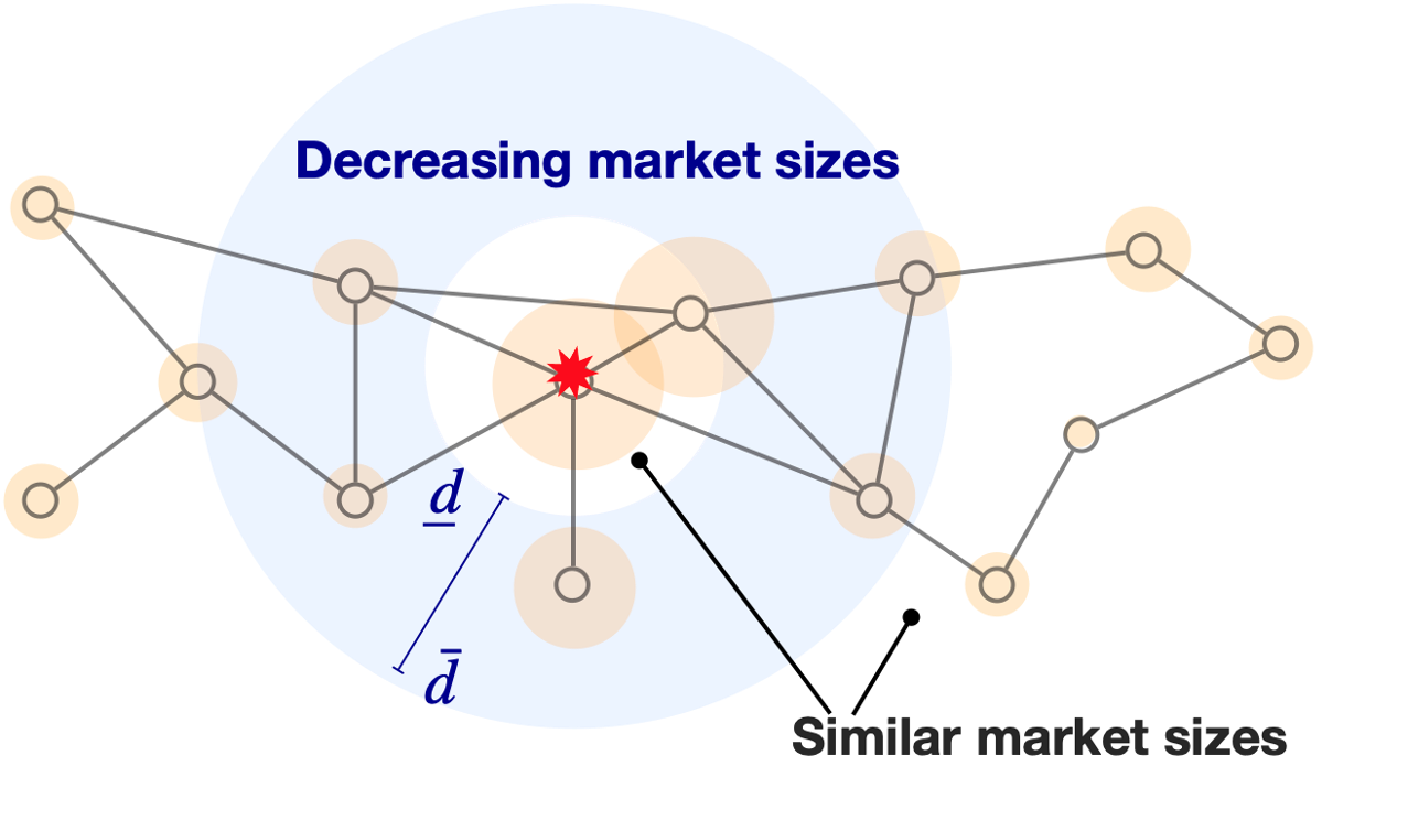
We define DD as the maximum distance of nodes that can be affected by demand shock in equilibrium, i.e. D=max⁡{d−K~,dK}D=\max\{d_{-\tilde{K}},d_{K}\}. Agents from any nodes with distances higher than DD will not move in equilibrium given any demand realization, and thus the market sizes of these nodes are irrelevant for information design. The following theorem shows that a monotone partitional information mechanism is optimal if there exists a monotone transition region, where nodes with distances between d¯\underline{d} and d¯\bar{d} have monotonically increasing or decreasing market sizes relative to their distances to node 00.

Theorem 1.

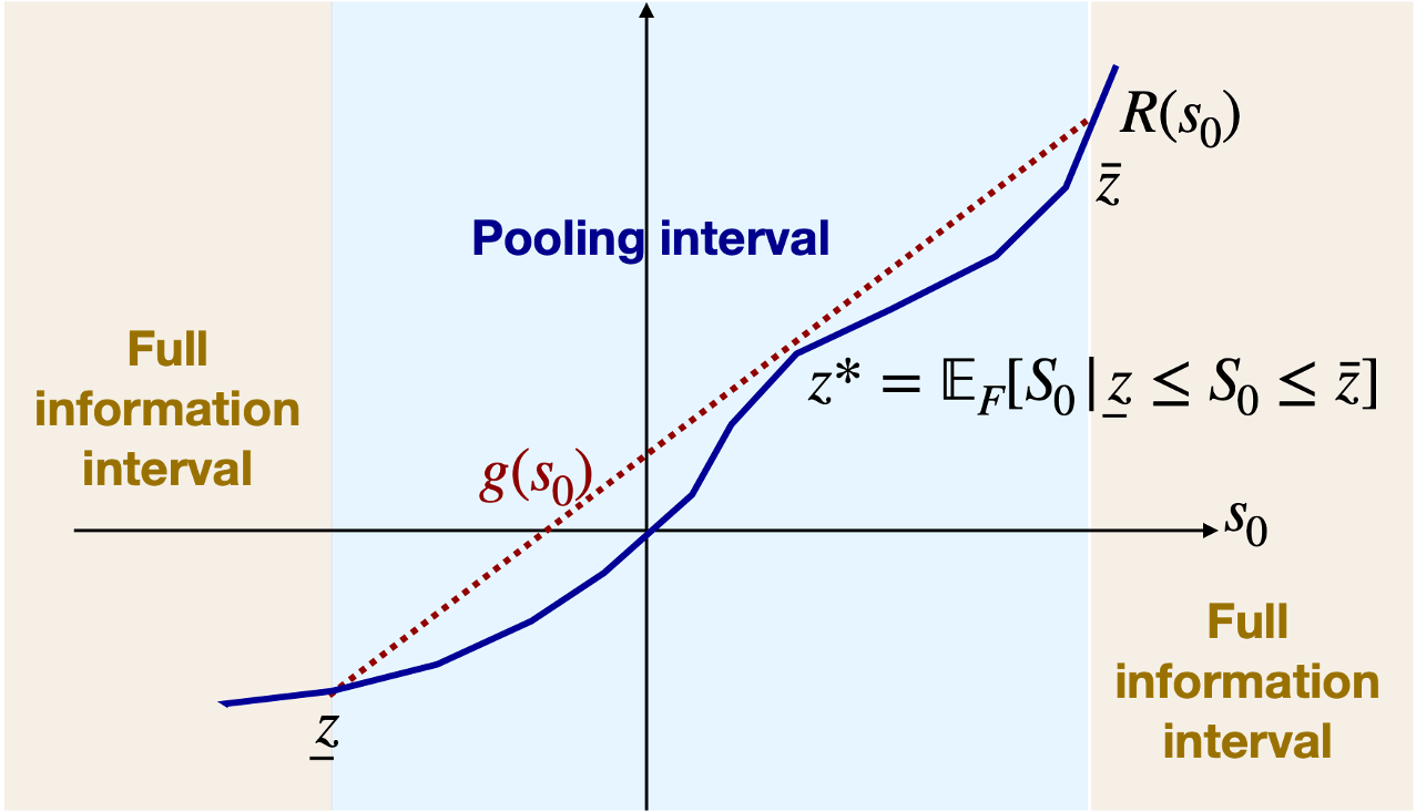
Under Assumptions 1 and 2, suppose that there exists 0≤d¯≤d¯≤D0\leq\underline{d}\leq\bar{d}\leq D such that nodes with distances less than d¯\underline{d} have similar market sizes, nodes with distances in [d¯,d¯][\underline{d},\bar{d}] have decreasing or increasing market sizes, and nodes with distances higher than d¯\bar{d} also have similar market sizes relative to distances. Given any prior distribution FF, there exists an optimal monotone partitional information mechanism with thresholds inf𝒮0≤z¯≤z¯≤sup𝒮0\inf\mathcal{S}_{0}\leq\underline{z}\leq\bar{z}\leq\sup\mathcal{S}_{0} that fully reveals states s0≤z¯s_{0}\leq\underline{z} and s0≥z¯s_{0}\geq\bar{z}, and pools states s0∈[z¯,z¯]s_{0}\in[\underline{z},\bar{z}] with posterior mean z∗=𝔼F​[S0|z¯≤S0≤z¯]z^{*}=\mathbb{E}_{F}[S_{0}|\underline{z}\leq S_{0}\leq\bar{z}]. Specifically,

  1. (i)

    z¯=z¯\underline{z}=\bar{z} if d¯=d¯\underline{d}=\bar{d}. That is, full information revelation is optimal if all nodes have similar market sizes relative to distances.

  2. (ii)

    z∗>𝔼F​[S0]z^{*}>\mathbb{E}_{F}[S_{0}] if nodes with distances in [d¯,d¯][\underline{d},\bar{d}] have decreasing market sizes relative to distances.

  3. (iii)

    z∗<𝔼F​[S0]z^{*}<\mathbb{E}_{F}[S_{0}] if nodes with distances in [d¯,d¯][\underline{d},\bar{d}] have increasing market sizes relative to distances.

Theorem 1 shows that the optimal information mechanism reveals at least partial demand information to agents and has a simple partitional structure with up to three intervals.88 8 Since the revenue function R⁡(s0)R(s_{0}) is piecewise linear, fully revealing state information is equivalent to revealing the regime interval in which the state realization resides. These intervals consist of one pooling interval between z¯\underline{z} and z¯\bar{z}, and two full information revelation intervals for demands below z¯\underline{z} and above z¯\bar{z}. When all market sizes are similar relative to distances to node 0 (case (i) as shown in Fig. 2(a)), maximum revenue is achieved by revealing all information, resulting in a degenerate pooling interval. In both cases (ii) and (iii) as shown in Figures 2(d)and 2(f), the optimal information mechanism includes a pooling interval. In case (ii) (resp. case (iii)), the pooling interval generates a posterior mean that induces agents to move to node 0 (resp. move away from node 0) when the transition region has decreasing (resp. increasing) market sizes.

To understand the intuition behind cases (ii) and (iii) and the value of pooling more clearly, consider a simple example with three nodes on a line, where node 00 is prone to demand shocks. Suppose nodes 11 and 22 with distances d1<d2d_{1}<d_{2} do not have similar market sizes, and one of them is small whereas the other one is large. Consider positive shocks at node 00, which always improve the platform’s revenues. If the shock is large enough to influence the resources only in the small market, then this will have only marginal impact on the revenue change rate at node 00, but if it influences the large market, then the revenue change rate becomes substantially larger (see Proposition 3). This implies that if nodes 11 and 22 exhibit increasing market sizes, then the revenue function in the positive shock regime is convex, but in the decreasing market sizes case it is concave. This (local) concavity of the revenue function implies that as opposed to revealing the state, with appropriate pooling the platform can ensure higher profits. Specifically, in the positive shock regime, with decreasing market sizes, when the state realization is relatively small, revealing the states induces a few resources to reposition to 00 preserving a relatively high price there. However, when the realization is large, revealing the state leads to too many resources to reposition to 00, and in some realizations it may even incentivize the resources in the further out small markets to move, thereby leading to excessively low prices. While in the former case, pooling may lower revenues, in the latter case, by eliminating low prices, it ensures higher revenues. Concavity of the revenue function ensures that the latter effect dominates, and the expected revenues are higher with pooling. With increasing market sizes, convexity in the positive shock regime may at first suggest that pooling should not help. However, it turns out that in this case, in the negative shock regime we have local concavity of the payoff function. Hence, appropriate pooling, once again, improves revenues.

The scenario of similar or monotone market sizes described in Theorem 1 are of practical interests. Empirical studies Dong et al. 2018; Dean and Kockelman 2021 have demonstrated that the requests of ride-hailing services are often higher in regions close to the central business districts, which have more jobs, services and other economic activities, and decrease in regions far away from the central business districts. In Theorem 1, case (i) corresponds to the scenario where all affected nodes are within or close to the central business district, and thus all nodes have similar market sizes. Additionally, case (ii) corresponds to the scenario where the shock affects a node within the central business district and affect nodes that are outside of the district, which have decreasing market sizes relative to distances. On the other hand, case (iii) corresponds to the scenario where the shock happens at a node that is far away from the central business district, and therefore nodes that are further away from node 0 have higher market sizes. Theorem 1 demonstrates that in both cases, a simple partitional information mechanism with one pooling interval is optimal.

Proof sketch. The proof of Theorem 1 builds on the duality theory of optimal information design introduced in Dworczak and Martini 2019. This duality theory demonstrates that the optimal posterior mean distribution G∗G^{*} can be constructed by finding an upper closure ν⁡(s0)\nu(s_{0}) of the objective function R⁡(s0)R(s_{0}) that satisfies (i) the function ν⁡(s0)\nu(s_{0}) is convex and ν⁡(s0)≥R⁡(s0)\nu(s_{0})\geq R(s_{0}); (ii) the expected value of ν⁡(s0)\nu(s_{0}) with respect to G∗G^{*} is the same as that with R⁡(s0)R(s_{0}); (iii) The optimal posterior G∗G^{*} is a mean preserving spread of the prior FF, and the support set of G∗G^{*} is a subset of {S0|ν⁡(s0)=R⁡(s0)}\{S_{0}|\nu(s_{0})=R(s_{0})\} (Lemma 7 in Appendix D).

Building on the general theory, we further show that the construction of such convex upper closure function is associated with the second-order properties (convexity or concavity) of the revenue function R⁡(s0)R(s_{0}). In our problem, the second order property of R⁡(s0)R(s_{0}) is governed by how the derivative of the linear revenue function changes from one equilibrium regime to another. From Proposition 3, we find that the changes of the derivatives depend on the market sizes of nodes that are affected. Since nodes are added to the affected set according to their distances to node 00, the change of derivatives depend on the changes of market sizes relative to the distances.

We show that under Assumptions 1 – 2 and the condition that market sizes are similar or monotone with respect to their distances to node 0, there exists at most one sub-interval of states [s¯0,s¯0][\underline{s}_{0},\bar{s}_{0}] such that R⁡(s0)R(s_{0}) is concave in [s¯0,s¯0][\underline{s}_{0},\bar{s}_{0}] and convex to the left or right of this interval (Lemma 6 in Appendix D). In particular, the sub-interval is empty and the function R⁡(s0)R(s_{0}) is convex if all nodes have similar market sizes with respect to distances. Thus, ν⁡(s0)=R⁡(s0)\nu(s_{0})=R(s_{0}), G∗=FG^{*}=F satisfy conditions (a) – (c) indicating that the optimal information mechanism is to fully reveal the demand realization (Fig. 2(b)).

Additionally, in cases (ii) (resp.(iii)), the concave subinterval results in a higher (resp. lower) posterior mean than the prior mean. We prove that in both cases, the convex closure function can be constructed as ν⁡(s0)=max⁡{g⁡(s0),R⁡(s0)}\nu(s_{0})=\max\{g(s_{0}),R(s_{0})\}, where g⁡(s0)g(s_{0}) is an affine function tangent to the concave piece of the revenue function R⁡(s0)R(s_{0}). We show that the optimal information mechanism exhibits a simple partitional structure with one pooling interval that associated with the interval of states such that ν⁡(s0)=g⁡(s0)\nu(s_{0})=g(s_{0}), and the remaining states out of this interval are fully revealed. The posterior mean of the pooled state equals to tangent point z∗z^{*}, which is higher than (resp. lower than) the prior mean in case (ii) (resp. case (iii)). In Fig. 2(f) and 2(d), we illustrate the pooling and revealing intervals, and the affine function ff associated with the optimal information mechanism for cases (ii) – (iii), respectively.

Refer to caption
(a)
Refer to caption
(b)
Refer to caption
(c)
Refer to caption
(d)
Refer to caption
(e)
Refer to caption
(f)
Figure 2: (a)-(b) Nodes with similar market sizes and convex revenue function associated with full information revelation mechanism; (c)-(d) Nodes with decreasing transition region and revenue function associated with one pooling interval; (e)-(f) Nodes with increasing transition region and revenue function associated with one pooling interval.

The next corollary shows that when all nodes have monotone market sizes relative to their distances, one full information revelation interval becomes degenerate.

Corollary 1.

If all nodes have monotonically decreasing (resp. increasing) market sizes relative to distances, then given any prior distribution FF, the optimal information mechanism pools states s0≥z¯s_{0}\geq\underline{z} (resp. s0≤z¯s_{0}\leq\bar{z}) such that z¯<𝔼F​[S0]\underline{z}<\mathbb{E}_{F}[S_{0}] (resp. z¯>𝔼F​[S0]\bar{z}>\mathbb{E}_{F}[S_{0}]) and fully reveal states s0<z¯s_{0}<\bar{z} (resp. s0>z¯s_{0}>\bar{z}).

Corollary 1 builds on Theorem 1: When all nodes have decreasing (resp. increasing) market sizes, the revenue function is concave (resp. convex) for s0>𝔼F​[S0]s_{0}>\mathbb{E}_{F}[S_{0}] and convex (resp. concave) for s0<𝔼F​[S0]s_{0}<\mathbb{E}_{F}[S_{0}]. Consequently, we show that one of the two full revelation region becomes empty, and the optimal information mechanism pool states above threshold z¯\underline{z} (resp. below z¯\bar{z}).

Furthermore, we show that when the commission rate rr exceeds a certain threshold, all market sizes are categorized as being similar as in (11). Therefore, full information revelation is optimal with high commission rate following case (i) in Theorem 1.

Corollary 2.

Under Assumptions 1 and 2, for any prior state distribution FF and any sequence of market sizes {si}i∈V\{s_{i}\}_{i\in V}, full information provision mechanism is optimal for any r>r¯r>\bar{r}, where

r¯=1−mini,j∈{V|di≠dj}⁡|di−djsi−sj|.\bar{r}=1-\min_{i,j\in\{V|d_{i}\neq d_{j}\}}\left|\frac{d_{i}-d_{j}}{s_{i}-s_{j}}\right|.

Finally, we present an algorithm to compute the thresholds z¯\bar{z} and z¯\underline{z} of the monotone partitional information mechanism.

Proposition 4.

Under Assumptions 1 and 2, suppose that there exists 0≤d¯≤d¯≤D0\leq\underline{d}\leq\bar{d}\leq D such that nodes with distances less than d¯\underline{d} or higher than d¯\bar{d} have similar market sizes relative to distances, and nodes with distances in [d¯,d¯][\underline{d},\bar{d}] have increasing or decreasing market sizes relative to distances. The thresholds of the pooling interval z¯,z¯\underline{z},\bar{z} and the posterior mean z∗z^{*} are computed by Algorithm 1.

Proposition 4 and Algorithm 1 build on the proof of Theorem 1. In particular, if the derivative of the linear revenue function in each regime is non-decreasing, then Algorithm 1 returns identical z¯\underline{z} and z¯\bar{z} indicating that the pooling interval is degenerate. Otherwise, we identify a concave interval from regime k¯\underline{k} to k¯\bar{k}. Building on Theorem 1, Algorithm 1 computes the pooling interval by searching for the affine function g⁡(s0)g(s_{0}) that is tangent to R⁡(s0)R(s_{0}). In particular, the algorithm starts with the affine function being the revenue function associated with regime k¯\underline{k}, and iteratively proceeds to regimes with increasing kk until k¯\bar{k}. In each iteration, the algorithm computes the interval thresholds as the intersection of the affine function and the revenue function, and computes the mean of the state within the corresponding interval. The algorithm terminates by finding the interval such that the state mean equals to the point, where the affine function is tangent to the revenue function. The proof of Theorem 1 ensures that such interval exists, and is the optimal pooling region.

Input: d​R​(s0)d​s0​[k]\frac{dR(s_{0})}{ds_{0}}[k] for k=−K~,−K~+1,…,−1,0,1,…,K−1,Kk=-\tilde{K},-\tilde{K}+1,\dots,-1,0,1,\dots,K-1,K.
if d​R​(s0)d​s0​[k]\frac{dR(s_{0})}{ds_{0}}[k] is non-decreasing for all kk then
z¯←𝔼F​[S0]\underline{z}\leftarrow\mathbb{E}_{F}[S_{0}], z¯←𝔼F​[S0]\bar{z}\leftarrow\mathbb{E}_{F}[S_{0}] else
k¯←mink{k|d​R​(s0)d​s0[k]>d​R​(s0)d​s0[k+1]}\underline{k}\leftarrow\min_{k}\left\{k\left|\frac{dR(s_{0})}{ds_{0}}[k]>\frac{dR(s_{0})}{ds_{0}}[k+1]\right.\right\}, k¯←maxk{k|d​R​(s0)d​s0[k−1]>d​R​(s0)d​s0[k]}\bar{k}\leftarrow\max_{k}\left\{k\left|\frac{dR(s_{0})}{ds_{0}}[k-1]>\frac{dR(s_{0})}{ds_{0}}[k]\right.\right\}
    j←k¯j\leftarrow\underline{k}
    while j≤k¯j\leq\bar{k} do
   
gj​(z)=d​R​(s0)d​s0​[j]​(z−s0​[j])+R⁡(s0​[j]).g_{j}(z)=\frac{dR(s_{0})}{ds_{0}}[j](z-s_{0}[j])+R(s_{0}[j]).
z¯[j]←max{z∈S0|z≤s0[j],gj(z)≥R(z)}\underline{z}[j]\leftarrow\max\left\{z\in S_{0}\left|z\leq s_{0}[j],\quad g_{j}(z)\geq R(z)\right.\right\}, z¯[j]←min{z∈S0|z≥s0[j+1],gj(z)≥R(z)}\bar{z}[j]\leftarrow\min\left\{z\in S_{0}\left|z\geq s_{0}[j+1],\quad g_{j}(z)\geq R(z)\right.\right\}.
       if 𝔼F​[S0|z¯​[j]≤S0≤z¯​[j]]≤s0​[j+1]\mathbb{E}_{F}[S_{0}|\underline{z}[j]\leq S_{0}\leq\bar{z}[j]]\leq s_{0}[j+1] then
      breakelse
      j←j+1j\leftarrow j+1.if 𝔼F​[S0|z¯​[j]≤S0≤z¯​[j]]≥s0​[j]\mathbb{E}_{F}[S_{0}|\underline{z}[j]\leq S_{0}\leq\bar{z}[j]]\geq s_{0}[j] then
z¯←z¯​[j]\underline{z}\leftarrow\underline{z}[j], z¯←z¯​[j]\bar{z}\leftarrow\bar{z}[j], z∗←𝔼F​[S0|z¯​[j]≤S0≤z¯​[j]]z^{*}\leftarrow\mathbb{E}_{F}[S_{0}|\underline{z}[j]\leq S_{0}\leq\bar{z}[j]]else
z∗←s0​[j]z^{*}\leftarrow s_{0}[j], and z¯,z¯\bar{z},\underline{z} are solutions of the following equations:
z∗\displaystyle z^{*} =𝔼F​[S0|z¯≤S0≤z¯],gγ​(z)=γ⁡(z−s0​[j])+R⁡(s0​[j]),d​R​(s0)d​s0​[j+1]≤γ≤d​R​(s0)d​s0​[j],\displaystyle=\mathbb{E}_{F}[S_{0}|\underline{z}\leq S_{0}\leq\bar{z}],~g_{\gamma}(z)=\gamma(z-s_{0}[j])+R(s_{0}[j]),~\frac{dR(s_{0})}{ds_{0}}[j+1]\leq\gamma\leq\frac{dR(s_{0})}{ds_{0}}[j],
z¯\displaystyle\underline{z} =max{z∈S0|z<s0[j],gγ(z)≥R(z)},z¯=min{z∈S0|z>s0[j],gγ(z)≥R(z)}.\displaystyle=\max\left\{z\in S_{0}\left|z<s_{0}[j],~g_{\gamma}(z)\geq R(z)\right.\right\},~\bar{z}=\min\left\{z\in S_{0}\left|z>s_{0}[j],~g_{\gamma}(z)\geq R(z)\right.\right\}.
Output: z¯,z¯,z∗\bar{z},\underline{z},z^{*}.
ALGORITHM 1 Computation of thresholds z¯,z¯\underline{z},\bar{z} in the optimal monotone partitional information mechanism.

4 Generalized results for single shock

4.1 Generalization of optimal partitional information mechanism

In this section, we drop Assumptions 1 and 2, and instead make the following assumption on the initial market balance – no agents have incentives to move across nodes. This assumption is without loss of generality since under any reasonable equilibrium model agents will always make repositioning decisions so that mm satisfies the balancedness condition before the platform reveals any information of demand realization.

Assumption 3 (Initial market balance).

The market is initially balanced in that no agents have incentive to move given the initial agent distribution mm, i.e.

(1−r)​(sj−βj​mj)−ci​j≤(1−r)​(si−βi​mi)≤(1−r)​(sj−βj​mj)+ci​j,∀i,j∈V∖{0},\displaystyle(1-r)(s_{j}-\beta_{j}m_{j})-c_{ij}\leq(1-r)(s_{i}-\beta_{i}m_{i})\leq(1-r)(s_{j}-\beta_{j}m_{j})+c_{ij},\quad\forall i,j\in V\setminus\{0\},
(1−r)​(si−βi​mi)−ci​0≤(1−r)​(𝔼F​(S0)−β0​m0)≤(1−r)​(si−βi​mi)+ci​0,∀i∈V∖{0},\displaystyle(1-r)(s_{i}-\beta_{i}m_{i})-c_{i0}\leq(1-r)(\mathbb{E}_{F}(S_{0})-\beta_{0}m_{0})\leq(1-r)(s_{i}-\beta_{i}m_{i})+c_{i0},\quad\forall i\in V\setminus\{0\},

where 𝔼F​[S0]=∫s0s0​𝑑F​(s0)\mathbb{E}_{F}[S_{0}]=\int_{s_{0}}s_{0}dF(s_{0}) is the prior mean of the state s0s_{0}.

We only describe the ideas of equilibrium characterization and regime computation in the main text. The formal algorithm of computing equilibrium regimes and complete characterization of equilibrium agent distribution and revenue function are included in Appendix C. Our characterization approach closely follows the one in the previous section, but we need to have slight modifications since we now impose a more permissive initial market balance condition. In particular, in the general case, the equilibrium regimes are jointly determined by the distance did_{i} and the price with the initial agent mass si−βi​mis_{i}-\beta_{i}m_{i} for all nodes. For each s0>𝔼F​[s0]s_{0}>\mathbb{E}_{F}[s_{0}], there exists a set of nodes Γ\Gamma, where agents move to node 0, and the agents from the remaining nodes V∖ΓV\setminus\Gamma do not move. Moreover, agents from a subset of nodes Γ†⊆Γ\Gamma^{\dagger}\subseteq\Gamma may entirely move to node 0 since the no depletion assumption is no longer imposed.

In Appendix C, we develop Algorithm 2 to compute equilibrium regimes for all s0≥𝔼F​[S0]s_{0}\geq\mathbb{E}_{F}[S_{0}]. The algorithm starts with regime 0, where both sets Γ⁡[0]\Gamma[0] and Γ†​[0]\Gamma^{\dagger}[0] are empty, and all agents stay at their origin nodes. As s0s_{0} increases, agents from node i∈V∖{0}i\in V\setminus\{0\} with the maximum initial payoff plus distance (i.e. (1−r)​(si−βi​mi)+di(1-r)(s_{i}-\beta_{i}m_{i})+d_{i}) start to move to node 0 in equilibrium of regime 11, and thus node ii is added to the set Γ⁡[1]\Gamma[1]. The regime threshold s0​[1]s_{0}[1] is computed as the state realization such that agents at node ii are indifferent between staying at ii and moving to node 00. Similarly, Algorithm 2 computes all possible equilibrium regimes k=1,…,Kk=1,\dots,K, where the regime change from kk to k+1k+1 occurs when either a node i∈arg​maxV∖Γ⁡[k]⁡(1−r)​(si−βi​mi)+dii\in\argmax_{V\setminus\Gamma[k]}(1-r)(s_{i}-\beta_{i}m_{i})+d_{i} is added to the set Γ⁡[k+1]\Gamma[k+1] or the price at node 00 surpasses the maximum payoff plus the distance (1−r)​si+di(1-r)s_{i}+d_{i} of a node in Γ⁡[k]\Gamma[k] so that all agents leave node ii (i.e. node ii is added into Γ†​[k+1]\Gamma^{\dagger}[k+1]). The algorithm terminates with regime KK such that all agents move to node 00. Since any node can only be added to Γ\Gamma and Γ†\Gamma^{\dagger} once, the maximum number of regimes K≤2​|V|K\leq 2|V|, and the algorithm terminates in less than 2​|V|2|V| iterations.

Likewise, for any s0<𝔼F​[S0]s_{0}<\mathbb{E}_{F}[S_{0}], agents at node 00 move to a subset of nodes Γ~\tilde{\Gamma}, while the remaining agents do not move. In particular, as s0s_{0} decreases, nodes are included into Γ~\tilde{\Gamma} in decreasing order of (1−r)​(si−βi​mi)−di(1-r)(s_{i}-\beta_{i}m_{i})-d_{i}. In Appendix C, Algorithm 3 computes the set Γ~​[k]\tilde{\Gamma}[k] for each regime −k=−1,…,−K~-k=-1,\dots,-\tilde{K}, and the regime boundaries {s0​[−k]}k=1K~\{s_{0}[-k]\}_{k=1}^{\tilde{K}}. Since each node is only added to Γ~\tilde{\Gamma} once, K~≤|V|\tilde{K}\leq|V| and the algorithm terminates in less than |V||V| iterations.

Based on the equilibrium characterization, we show that the platform’s revenue function is a continuous piecewise linear function of s0s_{0} and the derivative of the linear piece d​R​(s0)d​s0​[k]\frac{dR(s_{0})}{ds_{0}}[k] depends on the sets Γ⁡[k]\Gamma[k] and Γ†​[k]\Gamma^{\dagger}[k] in regime kk, and Γ~​[−k]\tilde{\Gamma}[-k] in regime −k-k (Proposition 7 in Appendix C). We next generalize Theorem 1 to provide verifiable conditions that guarantee the existence of an optimal monotone partitional information mechanism under the following mild regularity condition of the revenue function R⁡(s0)R(s_{0}).99 9 It can be seen that this condition generically holds. More precisely, for any revenue function that violates Assumption 4 with ka,kb,kck_{a},k_{b},k_{c}, a slight perturbation of agent mass mim_{i} for i∈Γ⁡[kc]i\in\Gamma[k_{c}] (or Γ~​[kc]\tilde{\Gamma}[k_{c}] if kc<0k_{c}<0) will make {(s0​[kj],R⁡(s0​[kj]))}j=a,b,c\{(s_{0}[k_{j}],R(s_{0}[k_{j}]))\}_{j=a,b,c} not lie on the same line, and thus leads to satisfaction of this condition.

Assumption 4.

There does not exist ka<kb<kck_{a}<k_{b}<k_{c} such that {(s0​[kj],R⁡(s0​[kj]))}j=a,b,c\{(s_{0}[k_{j}],R(s_{0}[k_{j}]))\}_{j=a,b,c} lie on the same line.

We define concave intervals of the revenue function R⁡(s0)R(s_{0}) as {[s0​[kℓ,a],s0​[kℓ,b]]}ℓ=1L\{[s_{0}[k_{\ell,a}],s_{0}[k_{\ell,b}]]\}_{\ell=1}^{L}, where −K~≤k1,a≤k1,b<k2,a≤k2,b<⋯<kL,a≤kL,b≤K-\tilde{K}\leq k_{1,a}\leq k_{1,b}<k_{2,a}\leq k_{2,b}<\cdots<k_{L,a}\leq k_{L,b}\leq K. The platform’s revenue function R⁡(s0)R(s_{0}) is strictly concave (resp. strictly convex) at s0​[k]s_{0}[k] if d​R​(s0)d​s0​[k−1]>(resp.<)​d​R​(s0)d​s0​[k]\frac{dR(s_{0})}{ds_{0}}[k-1]>(\text{resp.}<)\frac{dR(s_{0})}{ds_{0}}[k] and concave (resp. convex) at s0​[k]s_{0}[k] if d​R​(s0)d​s0​[k−1]≥(resp.≤)​d​R​(s0)d​s0​[k]\frac{dR(s_{0})}{ds_{0}}[k-1]\geq(\text{resp.}\leq)\frac{dR(s_{0})}{ds_{0}}[k]. For each interval ℓ\ell, the revenue function is strictly concave at s0​[kℓ,a]s_{0}[k_{\ell,a}] and s0​[kℓ,b]s_{0}[k_{\ell,b}], and concave for all s0​[k]s_{0}[k] with kℓ,a<k<kℓ,bk_{\ell,a}<k<k_{\ell,b}. Moreover, R⁡(s0)R(s_{0}) is convex for all kℓ,b<k<kℓ+1,ak_{\ell,b}<k<k_{\ell+1,a} and strictly convex for at least one kℓ,b<k^<kℓ+1,ak_{\ell,b}<\hat{k}<k_{\ell+1,a}.1010 10 This condition is to ensure that two cannot intervals cannot be combined into a single concave interval.

Before presenting the result, we first introduce the four conditions (C1) – (C4):

(C1) L≤1L\leq 1, i.e. the revenue function has at most one concave interval.

(C2) There does not exist ℓ<ℓ′\ell<\ell^{\prime} such that

d​R​(s0)d​s0​[kℓ,a−1]​(s0−s0​[kℓ,a])+R⁡(s0​[kℓ,a])−R⁡(s0)≥0,∀s0∈[s0​[kℓ′,a],s0​[kℓ′,b]],\displaystyle\frac{dR(s_{0})}{ds_{0}}[k_{\ell,a}-1]\left(s_{0}-s_{0}[k_{\ell,a}]\right)+R\left(s_{0}[k_{\ell,a}]\right)-R(s_{0})\geq 0,\quad\forall s_{0}\in\left[s_{0}[k_{\ell^{\prime},a}],s_{0}[k_{\ell^{\prime},b}]\right], (13a)
d​R​(s0)d​s0​[kℓ′,b]​(s0−s0​[kℓ′,b])+R⁡(s0​[kℓ′,b])−R⁡(s0)≥0,∀s0∈[s0​[kℓ,a],s0​[kℓ,b]],\displaystyle\frac{dR(s_{0})}{ds_{0}}[k_{\ell^{\prime},b}]\left(s_{0}-s_{0}[k_{\ell^{\prime},b}]\right)+R\left(s_{0}[k_{\ell^{\prime},b}]\right)-R(s_{0})\geq 0,\quad\forall s_{0}\in\left[s_{0}[k_{\ell,a}],s_{0}[k_{\ell,b}]\right], (13b)
∃s0∈[s0​[kℓ′,a],s0​[kℓ′,b]],s.t.d​R​(s0)d​s0​[kℓ,b]​(s0−s0​[kℓ,b])+R⁡(s0​[kℓ,b])−R⁡(s0)<0,\displaystyle\exists s_{0}\in\left[s_{0}[k_{\ell^{\prime},a}],s_{0}[k_{\ell^{\prime},b}]\right],\quad s.t.\quad\frac{dR(s_{0})}{ds_{0}}[k_{\ell,b}]\left(s_{0}-s_{0}[k_{\ell,b}]\right)+R\left(s_{0}[k_{\ell,b}]\right)-R(s_{0})<0, (13c)
∃s0∈[s0​[kℓ,a],s0​[kℓ,b]],s.t.d​R​(s0)d​s0​[kℓ′,a−1]​(s0−s0​[kℓ′,a])+R⁡(s0​[kℓ′,a])−R⁡(s0)<0.\displaystyle\exists s_{0}\in\left[s_{0}[k_{\ell,a}],s_{0}[k_{\ell,b}]\right],\quad s.t.\quad\frac{dR(s_{0})}{ds_{0}}[k_{\ell^{\prime},a}-1]\left(s_{0}-s_{0}[k_{\ell^{\prime},a}]\right)+R\left(s_{0}[k_{\ell^{\prime},a}]\right)-R(s_{0})<0. (13d)

The following lemma shows that when condition (C2) is not satisfied (i.e. there exists ℓ<ℓ′\ell<\ell^{\prime} that satisfy (13)), there exists a unique linear function that is tangent to the concave intervals ℓ\ell and ℓ′\ell^{\prime} of R⁡(s0)R(s_{0}). Otherwise, such linear tangent function does not exist.

Lemma 2.

For any ℓ<ℓ′\ell<\ell^{\prime}, there exists a unique linear function g⁡(z)=γ​z+λg(z)=\gamma z+\lambda such that g⁡(s0​[kℓ∗])=R⁡(s0​[kℓ∗]),g⁡(s0​[kℓ′∗])=R⁡(s0​[kℓ′∗])g(s_{0}[k_{\ell}^{*}])=R(s_{0}[k_{\ell}^{*}]),\quad g(s_{0}[k_{\ell^{\prime}}^{*}])=R(s_{0}[k_{\ell^{\prime}}^{*}]) for some kℓ,a≤kℓ∗≤kℓ,bk_{\ell,a}\leq k_{\ell}^{*}\leq k_{\ell,b} and kℓ′,a≤kℓ′∗≤kℓ′,bk_{\ell^{\prime},a}\leq k_{\ell^{\prime}}^{*}\leq k_{\ell^{\prime},b} and γ∈[d​R​(s0)d​s0​[kℓ∗],d​R​(s0)d​s0​[kℓ∗−1]]∩[d​R​(s0)d​s0​[kℓ′∗],d​R​(s0)d​s0​[kℓ′∗−1]]\gamma\in[\frac{dR(s_{0})}{ds_{0}}[k_{\ell}^{*}],\frac{dR(s_{0})}{ds_{0}}[k_{\ell}^{*}-1]]\cap[\frac{dR(s_{0})}{ds_{0}}[k_{\ell^{\prime}}^{*}],\frac{dR(s_{0})}{ds_{0}}[k_{\ell^{\prime}}^{*}-1]] if and only if (13) is satisfied.

(C3) For any pair of concave intervals ℓ<ℓ′\ell<\ell^{\prime} that satisfies (13), consider the associated affine function g⁡(z)g(z) and x=s0​[kℓ∗]x=s_{0}[k_{\ell}^{*}] (resp. y=s0​[kℓ′∗]y=s_{0}[k_{\ell^{\prime}}^{*}]) that satisfies R⁡(x)=g⁡(x)R(x)=g(x), R⁡(y)=g⁡(y)R(y)=g(y). Define z¯ℓ=max⁡{z<x|R⁡(z)≥g⁡(z)}\underline{z}_{\ell}=\max\{z<x|R(z)\geq g(z)\} and z¯ℓ′=min⁡{z>y|R⁡(z)≤g⁡(z)}\bar{z}_{\ell^{\prime}}=\min\{z>y|R(z)\leq g(z)\}. Then, either x,y<𝔼F​[S0],z¯ℓ′=sup𝒮0x,y<\mathbb{E}_{F}[S_{0}],\bar{z}_{\ell^{\prime}}=\sup\mathcal{S}_{0} or x,y>𝔼F​[S0],z¯ℓ=inf𝒮0x,y>\mathbb{E}_{F}[S_{0}],\underline{z}_{\ell}=\inf\mathcal{S}_{0}.

(C4) For any pair of concave intervals ℓ<ℓ′\ell<\ell^{\prime} that satisfy (13), and g⁡(z)g(z), xx, yy, z¯ℓ\underline{z}_{\ell} and z¯ℓ′\bar{z}_{\ell^{\prime}} defined as in (C3),

∫[z¯ℓ,y]z​𝑑F​(z)≥x,∫[x,z¯ℓ′]z​𝑑F​(z)≤y,(F−1​(z~)−x)​z~≥∫z¯ℓF−1​(z~)(F⁡(z)−F⁡(z¯ℓ))​𝑑z,\displaystyle\int_{[\underline{z}_{\ell},y]}zdF(z)\geq x,\quad\int_{[x,\bar{z}_{\ell^{\prime}}]}zdF(z)\leq y,\quad\left(F^{-1}\left(\tilde{z}\right)-x\right)\tilde{z}\geq\int_{\underline{z}_{\ell}}^{F^{-1}\left(\tilde{z}\right)}(F(z)-F(\underline{z}_{\ell}))dz, (14)

where

z~\displaystyle\tilde{z} =y​F​(z¯ℓ′)−x​F​(z¯ℓ)−z∗y−x,z∗=∫z¯ℓz¯ℓ′z​𝑑F​(z).\displaystyle=\frac{yF(\bar{z}_{\ell^{\prime}})-xF(\underline{z}_{\ell})-z^{*}}{y-x},\qquad z^{*}=\int_{\underline{z}_{\ell}}^{\bar{z}_{\ell^{\prime}}}zdF(z). (15)
Proposition 5.

There exists an optimal information mechanism that is monotone partitional if any of the four conditions (C1) – (C4) is satisfied.

Proposition 5 provides four verifiable conditions on the revenue function RR and the prior FF that guarantee the optimality of monotone partitional information mechanism. Among the four conditions, (C1) – (C2) only concern the revenue function, while (C3) – (C4) set conditions on RR and FF jointly.

In particular, (C1) ensures that the revenue function has at most one concave interval so that the optimal information mechanism can have at most one pooling region – recall that cases (i) – (iii) in Theorem 1 satisfy this condition. (C2) ensures that we cannot find an affine function that is tangent with two concave intervals. The theory of optimal information design shows that the existence of such affine functions indicates that the optimal information mechanism may contain double-interval structures that are not monotone – pooling high and low states in the interval to generate one posterior mean, and pooling the remaining states in the middle to generate another posterior mean. Specifically, the two posterior means take values of the two tangent points Candogan 2019; Dworczak and Martini 2019; Arieli et al. 2023. Both (C1) and (C2) ensure the optimality of monotone partitional mechanism by ruling out the existence of such affine functions. Thus, these two conditions are equivalent to the “affine closure” condition of Dworczak and Martini 2019 for the optimality of monotone partitional mechanisms, and they are easy to verify given the piecewise linear payoff struture in our problem.

Moreover, Proposition 5 extends the result in Dworczak and Martini 2019 by providing two other conditions (C3) – (C4) that allow the revenue function not to be affine closed, but can still guarantee the optimality of monotone partitional mechanism. Here, (C3) ensures that any posterior mean distribution that generates the two posterior mean values associated with the tangent points cannot be mean preserving spread of the prior, and thus is infeasible. Additionally, (C4) characterizes conditions on the prior FF to ensure that no feasible double-interval structure can be constructed to generate posterior means associated with any pair of tangent points, and we show that in that case the optimal information mechanism is necessarily monotone partitional.

4.2 Computing optimal information mechanism

In this section, we present the approach of computing an optimal information mechanism. We first show that any two posterior mean distributions lead to the same revenue if they induce the same expected posterior mean value and probability in each equilibrium regime, where the revenue function is linear.

Lemma 3.

For any two information mechanisms with posterior mean distribution GG and G′G^{\prime} such that for all k=−K~,…,Kk=-\tilde{K},\dots,K,

∫s0​[k−1]s0​[k]z​𝑑G​(z)=∫s0​[k−1]s0​[k]z​d​G′​(z),G⁡(s0​[k])−G⁡(s0​[k−1])=G′​(s0​[k])−G′​(s0​[k−1]),\displaystyle\int_{s_{0}[k-1]}^{s_{0}[k]}zdG(z)=\int_{s_{0}[k-1]}^{s_{0}[k]}zdG^{\prime}(z),\quad G(s_{0}[k])-G(s_{0}[k-1])=G^{\prime}(s_{0}[k])-G^{\prime}(s_{0}[k-1]),

we have RG=RG′R_{G}=R_{G^{\prime}}, where RGR_{G} (RG′R_{G^{\prime}}) is the platform’s revenue induced by the posterior mean distribution GG (resp. G′G^{\prime}).

The proof of Lemma 3 leverages the fact that revenue function R⁡(s0)R(s_{0}) is a continuous and piecewise linear function of s0s_{0}. Thus, the revenue only depends on the posterior mean of the state yk=∫s0​[k−1]s0​[k]z​𝑑G​(z)/(G⁡(s0​[k])−G⁡(s0​[k−1]))y_{k}=\int_{s_{0}[k-1]}^{s_{0}[k]}zdG(z)/(G(s_{0}[k])-G(s_{0}[k-1])) and the probability of inducing this posterior mean pk=G⁡(s0​[k])−G⁡(s0​[k−1])p_{k}=G(s_{0}[k])-G(s_{0}[k-1]) in each regime kk, rather than the exact posterior mean distribution GG. That is, any two posterior mean distributions that induce the same tuples {(pk,yk)}k=−K~K\{(p_{k},y_{k})\}_{k=-\tilde{K}}^{K} achieve the same revenue. The following proposition further shows that the optimal {(pk,yk)}k=−K~K\{(p_{k},y_{k})\}_{k=-\tilde{K}}^{K} can be computed by a convex optimization program.

Proposition 6.

The tuple {(pk,yk)}k=−K~K\{(p_{k},y_{k})\}_{k=-\tilde{K}}^{K} associated with the optimal information mechanism can be computed as an optimal solution of the following convex program:

maxp,y\displaystyle\max_{p,y}~ ∑k=−K~Kpk​R​(yk/pk),\displaystyle\sum_{k=-\tilde{K}}^{K}p_{k}R(y_{k}/p_{k}),
s.t.\displaystyle s.t.\quad ∑j=−K~kyj≤∫1−∑j=−K~kpj1F−1(x)dx,∀k=−K~,…,K,\displaystyle\sum_{j=-\tilde{K}}^{k}y_{j}\leq\int_{1-\sum_{j=-\tilde{K}}^{k}p_{j}}^{1}F^{-1}(x)dx,\quad\forall k=-\tilde{K},\dots,K, (16a)
s0[k−1]pk≤yk≤s0[k]pk,∀k=−K~,…,K,\displaystyle s_{0}[k-1]p_{k}\leq y_{k}\leq s_{0}[k]p_{k},\quad\forall k=-\tilde{K},\dots,K, (16b)
∑k=−K~Kpk=1,pk≥0,∀k=−K~,…,K.\displaystyle\sum_{k=-\tilde{K}}^{K}p_{k}=1,\quad p_{k}\geq 0,\quad\forall k=-\tilde{K},\dots,K. (16c)

Proposition 6 builds on Lemma 3 and the convex optimization framework developed in Candogan 2019. In particular, Candogan 2019 demonstrated that the optimal information mechanism can be constructed from an optimal {(pk,yk)}k=−K~K\{(p_{k},y_{k})\}_{k=-\tilde{K}}^{K}, where each kk with probability mass pk>0p_{k}>0 is associated with a posterior mean yk/pky_{k}/p_{k} given the optimal information mechanism. Moreover, the tightness of constraint (16a) indicates whether or not each posterior mean is induced by a single pooling interval or by a double-interval structure, and the interval thresholds can be explicitly constructed from the optimal {(pk,yk)}k=−K~K\{(p_{k},y_{k})\}_{k=-\tilde{K}}^{K}. The details closely follow Candogan 2019; Candogan and Strack 2021, and are omitted for brevity.

References

  • Alizamir et al. [2020] Saed Alizamir, Francis de Véricourt, and Shouqiang Wang. Warning against recurring risks: An information design approach. Management Science, 66(10):4612–4629, 2020.
  • Arieli et al. [2023] Itai Arieli, Yakov Babichenko, Rann Smorodinsky, and Takuro Yamashita. Optimal persuasion via bi-pooling. Theoretical Economics, 18(1):15–36, 2023.
  • Banerjee et al. [2022] Siddhartha Banerjee, Daniel Freund, and Thodoris Lykouris. Pricing and optimization in shared vehicle systems: An approximation framework. Operations Research, 70(3):1783–1805, 2022.
  • Bertsimas and Tsitsiklis [1997] Dimitris Bertsimas and John N Tsitsiklis. Introduction to linear optimization, volume 6. Athena scientific Belmont, MA, 1997.
  • Bimpikis et al. [2019] Kostas Bimpikis, Ozan Candogan, and Daniela Saban. Spatial pricing in ride-sharing networks. Operations Research, 67(3):744–769, 2019.
  • Blackwell [1953] David Blackwell. Equivalent comparisons of experiments. The annals of mathematical statistics, pages 265–272, 1953.
  • Candogan [2019] Ozan Candogan. Persuasion in networks: Public signals and k-cores. In Proceedings of the 2019 ACM Conference on Economics and Computation, pages 133–134, 2019.
  • Candogan [2020] Ozan Candogan. On information design with spillovers. Available at SSRN 3537289, 2020.
  • Candogan [2022] Ozan Candogan. Persuasion in networks: Public signals and cores. Operations Research, 70(4):2264–2298, 2022.
  • Candogan and Drakopoulos [2020] Ozan Candogan and Kimon Drakopoulos. Optimal signaling of content accuracy: Engagement vs. misinformation. Operations Research, 68(2):497–515, 2020.
  • Candogan and Gurkan [2023] Ozan Candogan and Huseyin Gurkan. Value of information design in supply chain management. Available at SSRN 4378997, 2023.
  • Candogan and Strack [2021] Ozan Candogan and Philipp Strack. Optimal disclosure of information to privately informed agents. Available at SSRN 3773326, 2021.
  • Das et al. [2017] Sanmay Das, Emir Kamenica, and Renee Mirka. Reducing congestion through information design. In 2017 55th annual allerton conference on communication, control, and computing (allerton), pages 1279–1284. IEEE, 2017.
  • De Véricourt et al. [2021] Francis De Véricourt, Huseyin Gurkan, and Shouqiang Wang. Informing the public about a pandemic. Management Science, 67(10):6350–6357, 2021.
  • Dean and Kockelman [2021] Matthew D Dean and Kara M Kockelman. Spatial variation in shared ride-hail trip demand and factors contributing to sharing: Lessons from chicago. Journal of Transport Geography, 91:102944, 2021.
  • Dong et al. [2018] Yongqi Dong, Shuofeng Wang, Li Li, and Zuo Zhang. An empirical study on travel patterns of internet based ride-sharing. Transportation research part C: emerging technologies, 86:1–22, 2018.
  • Drakopoulos et al. [2018] Kimon Drakopoulos, Shobhit Jain, and Ramandeep S Randhawa. Persuading customers to buy early: The value of personalized information provisioning. Available at SSRN 3191629, 2018.
  • Dworczak and Martini [2019] Piotr Dworczak and Giorgio Martini. The simple economics of optimal persuasion. Journal of Political Economy, 127(5):1993–2048, 2019.
  • Gentzkow and Kamenica [2016] Matthew Gentzkow and Emir Kamenica. A rothschild-stiglitz approach to bayesian persuasion. American Economic Review, 106(5):597–601, 2016.
  • Gur et al. [2019] Yonatan Gur, Gregory Macnamara, and Daniela Saban. On the disclosure of promotion value in platforms with learning sellers. arXiv preprint arXiv:1911.09256, 2019.
  • Johari et al. [2019] Ramesh Johari, Bar Light, and Gabriel Weintraub. Quality selection in two-sided markets: A constrained price discrimination approach. arXiv preprint arXiv:1912.02251, 2019.
  • Kolotilin [2018] Anton Kolotilin. Optimal information disclosure: A linear programming approach. Theoretical Economics, 13(2):607–635, 2018.
  • Küçükgül et al. [2022] Can Küçükgül, Özalp Özer, and Shouqiang Wang. Engineering social learning: Information design of time-locked sales campaigns for online platforms. Management Science, 68(7):4899–4918, 2022.
  • Lingenbrink and Iyer [2018] David Lingenbrink and Krishnamurthy Iyer. Signaling in online retail: Efficacy of public signals. Available at SSRN 3179262, 2018.
  • Lingenbrink and Iyer [2019] David Lingenbrink and Krishnamurthy Iyer. Optimal signaling mechanisms in unobservable queues. Operations Research, 67(5):1397–1416, 2019. ISSN 0030-364X. doi: 10.1287/opre.2018.1819.
  • Meigs et al. [2020] Emily Meigs, Francesca Parise, Asuman Ozdaglar, and Daron Acemoglu. Optimal dynamic information provision in traffic routing. arXiv preprint arXiv:2001.03232, 2020.
  • Papanastasiou et al. [2018] Yiangos Papanastasiou, Kostas Bimpikis, and Nicos Savva. Crowdsourcing exploration. Management Science, 64(4):1727–1746, 2018.
  • Shah et al. [2022] Sohil Shah, Saurabh Amin, and Patrick Jaillet. Optimal information provision for strategic hybrid workers. In 2022 IEEE 61st Conference on Decision and Control (CDC), pages 3807–3814. IEEE, 2022.
  • Tavafoghi and Teneketzis [2017] Hamidreza Tavafoghi and Demosthenis Teneketzis. Informational incentives for congestion games. In 2017 55th Annual Allerton Conference on Communication, Control, and Computing (Allerton), pages 1285–1292. IEEE, 2017.
  • Vasserman et al. [2015] Shoshana Vasserman, Michal Feldman, and Avinatan Hassidim. Implementing the wisdom of waze. In Twenty-Fourth International Joint Conference on Artificial Intelligence, 2015.
  • Wu and Amin [2019] Manxi Wu and Saurabh Amin. Information design for regulating traffic flows under uncertain network state. In 2019 57th Annual Allerton Conference on Communication, Control, and Computing (Allerton), pages 671–678. IEEE, 2019.
  • Yang et al. [2019] Pu Yang, Krishnamurthy Iyer, and Peter Frazier. Information design in spatial resource competition. arXiv preprint arXiv:1909.12723, 2019.

Appendix A Discussion: Computing best partitional mechanisms

In earlier sections we identified conditions under which partitional mechanisms are optimal. In this section we focus on more general settings where they are not optimal. Due to their simple and intuitive features, from a practical point of view, it may still be of interest to identify the best partitional mechanism in such settings. We provide an approach for obtaining (near-optimal) partitional mechanisms.

To this end, we first discretize the state space that induces ϵ\epsilon increments in the quantile space. We assume that we have access to an oracle that evaluates the inverse CDF function at the desired point, though the results go through even if these can be only approximately computed. We then argue that the dynamic programming (DP) approach of Candogan 2020 applies in this setting to derive the optimal partitional mechanism whose cutoffs are restricted to these points. It is easy to see that the payoffs are Lipshitz continuous in the cutoffs of the partitional mechanism. This, together with the fact that our DP runs in polynomial time in 1/ϵ1/\epsilon ensures that the resulting algorithm is a fully polynomial-time approximation scheme (FPTAS). We first describe the approach for the single shock case, and then discuss its extensions to the multiple shock case.

Let cℓ=F−1​(ϵ​ℓ)c_{\ell}=F^{-1}(\epsilon\ell) for k∈ℐ:={0,…,⌊1/ϵ⌋}k\in{\cal I}:=\{0,\dots,\lfloor 1/\epsilon\rfloor\}. If cℓ≠1c_{\ell}\neq 1 for any ℓ\ell, then let c⌊1/ϵ⌋+1=1c_{\lfloor 1/\epsilon\rfloor+1}=1. Define the set of feasible cutoffs as {cℓ},\{c_{\ell}\}, and the associated index set by ℐ{\cal I}. Let max⁡ℐ=L\max{\cal I}=L For any ℓ1,ℓ2∈ℐ\ell_{1},\ell_{2}\in{\cal I} where ℓ1≤ℓ2\ell_{1}\leq\ell_{2}, let p⁡(ℓ1,ℓ2)=F⁡(cℓ2)−F⁡(cℓ1)p(\ell_{1},\ell_{2})=F(c_{\ell_{2}})-F(c_{\ell_{1}}), and w(ℓ1,ℓ2)=R(𝔼[s0|s0∈[cℓ1,cℓ2])/p(ℓ1,ℓ2)w(\ell_{1},\ell_{2})=R\left(\mathbb{E}[s_{0}|s_{0}\in[c_{\ell_{1}},c_{\ell_{2}}]\right)\bigg/p(\ell_{1},\ell_{2}). Suppose that we choose indices ℐc={ℓ0,ℓ1,…,ℓK}⊆ℐ{\cal I}_{c}=\{\ell_{0},\ell_{1},\dots,\ell_{K}\}\subseteq{\cal I} with ℓ0=0\ell_{0}=0, ℓK=L\ell_{K}=L. In this case, it can be seen that the expected payoff of the designer can be expressed as ∑k=1Kw⁡(ℓk−1,ℓk)\sum_{k=1}^{K}w(\ell_{k-1},\ell_{k}). It can be readily seen that any feasible partitional mechanism (with cutoffs in {ck}k∈ℐ\{c_{k}\}_{k\in{\cal I}}) can be associated with an index set of the type ℐc{\cal I}_{c}, the problem reduces to finding the best such set.

However, this problem can naturally be formulated as a DP. Specifically, suppose that we sequentially add indices to ℐc{\cal I}_{c} starting with {L}\{L\}, at each step adding a new index that is smaller than the previously added ones, and stopping once index 0=min⁡ℐ0=\min{\cal I} is added to ℐc{\cal I}_{c}. Suppose we have a set ℐc={ℓk+1,…,ℓK}{\cal I}_{c}=\{\ell_{k+1},\dots,\ell_{K}\} with ℓk+1<⋯<ℓK=L\ell_{k+1}<\dots<\ell_{K}=L, of indices that are already chosen, and suppose that we next add index ℓk<ℓk+1\ell_{k}<\ell_{k+1} to ℐc{\cal I}_{c}. Denote the stage payoff for adding an index ℓk\ell_{k} to the current set by w⁡(ℓk,ℓk+1)w(\ell_{k},\ell_{k+1}), and denote the continuation payoff by V⁡(ℓk)V(\ell_{k}). It can be readily seen that the objective value associated with the optimal mechanism (with cutoffs in {ck}k∈ℐ\{c_{k}\}_{k\in{\cal I}}) is V⁡(L)V(L), and we have the following Bellman equation:

V⁡(ℓk)=maxℓ<ℓk|ℓ∈ℐ⁡V⁡(ℓ)+w⁡(ℓ,ℓk).V(\ell_{k})=\max_{\ell<\ell_{k}|\ell\in{\cal I}}V(\ell)+w(\ell,\ell_{k}). (17)

This equation can be solved via standard dynamic programming techniques, and yield the optimal partitional mechanism with cutoffs restricted to ℐ{\cal I}, which in turn yields an FPTAS as explained earlier.1111 11 See Candogan 2020 for a detailed algorithm description. The aforementioned paper’s algorithm also applies in richer settings where different groups of agents have access to different signals, and information can spill over from one agent to another according to an underlying communication network.

In the discussion above, we did not specify which of the assumptions (Assumption 1,2, 3) should be imposed. This is deliberate. If these assumptions hold, then the R⁡(⋅)R(\cdot) function can be obtained in closed form, and it can be used to construct w⁡(⋅,⋅)w(\cdot,\cdot) as described earlier. Otherwise, for any ℓ1,ℓ2∈ℐ\ell_{1},\ell_{2}\in{\cal I} and the posterior mean level 𝔼⁡[s0|s0∈[cℓ1,cℓ2]]\mathbb{E}[s_{0}|s_{0}\in[c_{\ell_{1}},c_{\ell_{2}}]] we can solve the optimization formulation in Proposition 1 to obtain the distribution of agents for different posterior mean levels that are induced by partitional mechanisms with cutoffs in {cℓ}ℓ∈ℐ\{c_{\ell}\}_{\ell\in{\cal I}}. We then evaluate the induced revenue. After solving these auxiliary optimization problems we evaluate the R⁡(⋅)R(\cdot) function at all relevant posterior mean levels and, in turn, construct the w⁡(⋅,⋅)w(\cdot,\cdot) function.

We next extend our approach to the multiple shock case. To start, we need to extend the definition of partitional information structures to the multiple shock case. A natural idea is to choose partitions for each {Si}\{S_{i}\} separately, and reveal the partition elements to which each SiS_{i} belongs. However, there is a fundamental difficulty: The number of possible signal realizations grows exponentially in the number of shock centers, thereby leading to computational difficulties when large number of nodes are impacted by shocks. This is to some extent expected, since in the aforementioned settings the designer’s payoff is piecewise linear with exponentially many pieces, and solving an optimization involving such a rich class of functions is nontrivial.

That said, there is a practically relevant version of the problem that is also tractable. Specifically, suppose that we have finitely many scenarios {σk}k∈Σ\{\sigma_{k}\}_{k\in\Sigma} and an associated probability distribution {ρk}k∈Σ\{\rho_{k}\}_{k\in\Sigma}, where Σ={1,…,D}\Sigma=\{1,\dots,D\}. Associated with scenario kk is a fixed shock vector νk\nu^{k}, and random variable θk\theta^{k} with distribution FkF^{k}. When this scenario is realized the price curve in node ii takes the form

pi​(qi)=si+θk​νik.p_{i}(q_{i})=s_{i}+\theta^{k}\nu^{k}_{i}.

In other words, when this scenario is realized the intercept of the price curve in each node is perturbed according to the vector νk\nu^{k}. Note that we do not make any restrictions on the entries of νk\nu^{k}. For instance, multiple entries can be nonzero, e.g., capturing the fact that multiple nodes simultaneously experience varying degrees of shocks (which in the ride-sharing application can capture some regions of the city jointly experiencing demand shocks, e.g., due to weather events or special events leading to demand surge in a wide area). We also allow for negative entries/shocks (that in the ride-sharing application can capture reduced demand in some areas while others are experiencing increased demand, e.g., due to shocks in the public transit system).

As before, we discretize the support of each θk\theta^{k} in a way that leads to ϵ\epsilon increments in the quantile space. Denote the corresponding cutoffs for scenario kk by {cℓk}ℓ\{c^{k}_{\ell}\}_{\ell}, and the associated index set by ℐk{\cal I}^{k}. For each scenario kk, and indices ℓ1,ℓ2∈ℐk\ell_{1},\ell_{2}\in{\cal I}^{k}, we compute the induced payoff of the platform when the posterior mean vector is 𝔼Fk​[s+θk​νk|θk∈[cℓ1,cℓ2]]\mathbb{E}_{F^{k}}[s+\theta^{k}\nu^{k}|\theta^{k}\in[c_{\ell_{1}},c_{\ell_{2}}]]. While, unlike the single shock case, this quantity is not possible to obtain in closed form, Proposition 1 still applies to characterize equilibrium agent distribution for each scenario and pairs of discretization indices (k,ℓ1,ℓ2)(k,\ell_{1},\ell_{2}).

We once again focus on partitional mechanisms. However, note that without the knowledge of the underlying scenario, the partitional structure is not very intuitive or practical.1212 12 For instance, suppose that two scenarios represent demand surging in two different parts of the city. Without revealing which scenario is realized it is not meaningful to reveal that the demand is in top, say, 20% of the possible levels. Motivated by this, we restrict attention to mechanisms that (i) reveal the scenario that is realized, and (ii) use partitional information structures to map state realization to signals for each scenario.

It can be readily seen that for such mechanisms, the design problem decouples over different scenarios. That is, the partition chosen for one scenario has no impact on the payoff obtained when another scenario is realized. As such, for each scenario we have a DP recursion of the type (17), where V⁡(⋅)V(\cdot) and w⁡(⋅,⋅)w(\cdot,\cdot) (and more fundamentally the revenue function R⁡(⋅)R(\cdot)) are now scenario-specific.

In short, the DP approached introduced earlier readily extends to multiple demand shock scenarios. This gives a simple and computationally efficient recipe for constructing practically relevant information disclosure mechanisms.

Appendix B Proofs of statements in Sections 2

Proof of Proposition 1. For any t∈𝒯t\in\mathcal{T}, Φ⁡(x|t)\Phi(x|t) is a potential function since:

d​Φ​(x|t)d​xi​j​(t)=(1−r)​(𝔼⁡[sj|t]−βj​qj​(t))−ci​j=ui​j​(x|t),∀i,j∈V.\displaystyle\frac{d\Phi(x|t)}{dx_{ij(t)}}=(1-r)(\mathbb{E}[s_{j}|t]-\beta_{j}q_{j}(t))-c_{ij}=u_{ij}(x|t),\quad\forall i,j\in V.

Therefore, following [ ] , we know that x∗x^{*} is a maximizer of the potential function.

Moreover, given any q∗​(t)q^{*}(t), since the associated equilibrium strategy x∗​(t)x^{*}(t) maximizes the potential function, x∗​(t)x^{*}(t) must be an optimal solution of the following problem:

minx∑i,j∈Vci​j​xi​j​(t),s.t.∑i∈Vxi​j(t)=q∗j(t),∀j∈V,∑j∈Vxi​j(t)=mi,∀i∈V,xi​j​(t)≥0,∀i,j∈V.\begin{split}\min_{x}\quad&\sum_{i,j\in V}c_{ij}x_{ij}(t),\\ s.t.\quad&\sum_{i\in V}x_{ij}(t)=q^{*}_{j}(t),\quad\forall j\in V,\\ &\sum_{j\in V}x_{ij}(t)=m_{i},\quad\forall i\in V,\\ &x_{ij}(t)\geq 0,\quad\forall i,j\in V.\end{split} (18)

From the duality theory, the optimal value ψ⁡(q∗|t)=∑i,j∈Vci​j​xi​j∗​(t)\psi(q^{*}|t)=\sum_{i,j\in V}c_{ij}x^{*}_{ij}(t) is a convex function of q∗​(t)q^{*}(t) (Theorem 5.1 on page 213 in Bertsimas and Tsitsiklis 1997). Moreover, we denote ϕ⁡(q|t)=(1−r)​∑i∈V∫0qi​(t)(𝔼⁡[si|t]−βj​z)​𝑑z\phi(q|t)=(1-r)\sum_{i\in V}\int_{0}^{q_{i}(t)}(\mathbb{E}[s_{i}|t]-\beta_{j}z)dz note that

∂2ϕ⁡(q|t)∂qi​∂qj={−(1−r)​βi,i=j,0,i≠j.\displaystyle\frac{\partial^{2}\phi(q|t)}{\partial q_{i}\partial q_{j}}=\left\{\begin{array}[]{ll}-(1-r)\beta_{i},&\quad i=j,\\ 0,&\quad i\neq j.\end{array}\right.

That is, ϕ⁡(q|t)\phi(q|t) is strictly concave in qq. We can re-write the potential function as a function of qq, ϕ⁡(q|t)−ψ⁡(q|t)\phi(q|t)-\psi(q|t), which is strictly concave in qq. Thus, the equilibrium agents’ distribution q∗​(t)q^{*}(t) is unique for all t∈𝒯t\in\mathcal{T}. □\square

Proof of Proposition 2. We note that the feasible set of the optimization problem (6) associated with F′F^{\prime} is super set of that associated with FF. Therefore, RG′∗≥RG∗R_{G^{{}^{\prime}*}}\geq R_{G^{*}}, where G′∗G^{{}^{\prime}*} (resp. G∗G^{*}) is the optimal posterior mean distribution given prior F′F^{\prime} (resp. FF). Moreover, since 𝔼F​[s0]=𝔼F′​[s0]\mathbb{E}_{F}[s_{0}]=\mathbb{E}_{F^{\prime}}[s_{0}], we have RF=R⁡(𝔼F​[s0])=R⁡(𝔼F′​[s0])=RF′R_{F}=R(\mathbb{E}_{F}[s_{0}])=R(\mathbb{E}_{F^{\prime}}[s_{0}])=R_{F^{\prime}}. Therefore, VF∗≤VF′∗V^{*}_{F}\leq V^{*}_{F^{\prime}}. □\square

Appendix C Equilibrium characterization for the single shock case

In this section, we provide a complete equilibrium characterization for the single shock case under Assumption 3.

The following lemma demonstrates structural properties of equilibrium strategy profile and agents’ distribution. In particular, for any s0>𝔼F​[s0]s_{0}>\mathbb{E}_{F}[s_{0}], that there exists an equilibrium strategy profile such that the nodes in the network are partitioned into three sets V=(V∖Γ)∪(Γ∖Γ†)∪Γ†V=(V\setminus\Gamma)\cup(\Gamma\setminus\Gamma^{\dagger})\cup\Gamma^{\dagger}, where agents from i∈(V∖Γ)i\in(V\setminus\Gamma) do not move, a fraction of agents from i∈(Γ∖Γ†)i\in(\Gamma\setminus\Gamma^{\dagger}) move to node 00 and the rest stay at node ii, and all agents from i∈Γ†i\in\Gamma^{\dagger} move to node 00 in equilibrium. Additionally, for any s0<𝔼F​[s0]s_{0}<\mathbb{E}_{F}[s_{0}], nodes are partitioned into two sets V=(V∖Γ~)∪Γ~V=(V\setminus\tilde{\Gamma})\cup\tilde{\Gamma} such that agents from node ii move to nodes in Γ~\tilde{\Gamma}, and agents from the rest of the network do not move.

Lemma 4.

For any s0>𝔼F​[s0]s_{0}>\mathbb{E}_{F}[s_{0}], the unique agents’ distribution in equilibrium q∗q^{*} satisfies:

qi∗=1βi​(si−s0+di1−r)+β0βi​q0∗∈(0,mi),∀i∈Γ∖Γ†,\displaystyle q^{*}_{i}=\frac{1}{\beta_{i}}\left(s_{i}-s_{0}+\frac{d_{i}}{1-r}\right)+\frac{\beta_{0}}{\beta_{i}}q^{*}_{0}\in(0,m_{i}),\quad\forall i\in\Gamma\setminus\Gamma^{\dagger}, (19a)
qi∗=0,∀i∈Γ†,\displaystyle q^{*}_{i}=0,\quad\forall i\in\Gamma^{\dagger}, (19b)
qi∗=mi,∀i∈V∖{Γ∪{0}},\displaystyle q^{*}_{i}=m_{i},\quad\forall i\in V\setminus\{\Gamma\cup\{0\}\}, (19c)

where

Γ={V|(1−r)​(si−βi​mi)+di<(1−r)​(s0−β0​q0∗)},\displaystyle\Gamma=\{V|(1-r)(s_{i}-\beta_{i}m_{i})+d_{i}<(1-r)(s_{0}-\beta_{0}q^{*}_{0})\}, (20a)
Γ†={V|(1−r)​si+di≤(1−r)​(s0−β0​q0∗)},\displaystyle\Gamma^{\dagger}=\{V|(1-r)s_{i}+d_{i}\leq(1-r)(s_{0}-\beta_{0}q^{*}_{0})\}, (20b)

and there exists an equilibrium strategy profile such that

x00∗=m0,xi​0∗=mi−qi∗,xi​i∗=qi∗,xi​j∗=0,∀i∈V∖{0},∀j∈V∖{0,i}.\displaystyle x^{*}_{00}=m_{0},\quad x^{*}_{i0}=m_{i}-q^{*}_{i},\quad x^{*}_{ii}=q^{*}_{i},\quad x^{*}_{ij}=0,\quad\forall i\in V\setminus\{0\},\quad\forall j\in V\setminus\{0,i\}. (21)

For any s0<𝔼F​[s0]s_{0}<\mathbb{E}_{F}[s_{0}], the unique agents’ distribution in equilibrium q∗q^{*} satisfies:

qi∗=1βi​(si−s0−di1−r)+β0βi​q0∗>mi,∀i∈Γ~,\displaystyle q^{*}_{i}=\frac{1}{\beta_{i}}\left(s_{i}-s_{0}-\frac{d_{i}}{1-r}\right)+\frac{\beta_{0}}{\beta_{i}}q^{*}_{0}>m_{i},\quad\forall i\in\tilde{\Gamma}, (22a)
qi∗=mi,∀i∈V∖{Γ~∪{0}},\displaystyle q^{*}_{i}=m_{i},\quad\forall i\in V\setminus\{\tilde{\Gamma}\cup\{0\}\}, (22b)

where

Γ~={V|(1−r)​(si−βi​mi)−di>(1−r)​(s0−β0​q0∗)},\displaystyle\tilde{\Gamma}=\{V|(1-r)(s_{i}-\beta_{i}m_{i})-d_{i}>(1-r)(s_{0}-\beta_{0}q^{*}_{0})\}, (23)

and there exists an equilibrium strategy profile such that

x0​i∗\displaystyle x^{*}_{0i} =qi∗−mi,∀i∈Γ~,x0​i∗=0,∀i∈V∖{0∪Γ~},x00∗=q0∗,\displaystyle=q^{*}_{i}-m_{i},\quad\forall i\in\tilde{\Gamma},\quad x^{*}_{0i}=0,\quad\forall i\in V\setminus\{0\cup\tilde{\Gamma}\},\quad x^{*}_{00}=q^{*}_{0}, (24a)
xi​i∗\displaystyle x^{*}_{ii} =mi,∀i∈V∖{0},xi​j∗=0,∀j∈V∖{0,i}.\displaystyle=m_{i},\quad\forall i\in V\setminus\{0\},\quad x^{*}_{ij}=0,\quad\forall j\in V\setminus\{0,i\}. (24b)

Furthermore, q0∗q^{*}_{0} increases in s0s_{0}.

Proof of Lemma 4. We first prove that given any s0>𝔼F​[s0]s_{0}>\mathbb{E}_{F}[s_{0}], agents originating from all nodes do not have incentive to deviate from their equilibrium strategy x∗x^{*} as in (21) given q∗q^{*} in (19). We first note that q∗q^{*} as in (19) ensures that

(1−r)​(si−βi​qi∗)=(1−r)​(s0−β0​q0∗)−di,∀i∈Γ∖Γ†.\displaystyle(1-r)(s_{i}-\beta_{i}q^{*}_{i})=(1-r)(s_{0}-\beta_{0}q^{*}_{0})-d_{i},\quad\forall i\in\Gamma\setminus\Gamma^{\dagger}. (25)

(1) For any i∈V∖{Γ∪{0}}i\in V\setminus\{\Gamma\cup\{0\}\}, we note that the payoff of staying at node ii is (1−r)​(si−βi​qi∗)=(1−r)​(si−βi​mi)(1-r)(s_{i}-\beta_{i}q^{*}_{i})=(1-r)(s_{i}-\beta_{i}m_{i}), which is higher or equal to (1−r)​(s0−β0​q0∗)−di(1-r)(s_{0}-\beta_{0}q^{*}_{0})-d_{i} – the expected payoff of moving to node 00. Thus, agents at node ii has no incentive to move to node 00 in equilibrium. Additionally, following (25), we have

(1−r)​(sj−βj​qj∗)−ci​j\displaystyle(1-r)(s_{j}-\beta_{j}q^{*}_{j})-c_{ij} =(1−r)​(s0−β0​q0∗)−dj−ci​j≤(a)(1−r)​(s0−β0​q0∗)−di\displaystyle=(1-r)(s_{0}-\beta_{0}q^{*}_{0})-d_{j}-c_{ij}\stackrel{{\scriptstyle(a)}}{{\leq}}(1-r)(s_{0}-\beta_{0}q^{*}_{0})-d_{i}
≤(1−r)​(si−βi​mi)=(1−r)​(si−βi​qi∗),∀j∈Γ,\displaystyle\leq(1-r)(s_{i}-\beta_{i}m_{i})=(1-r)(s_{i}-\beta_{i}q^{*}_{i}),\quad\forall j\in\Gamma,

where (a) is due to the triangular inequality of distances, i.e. di≤dj+ci​jd_{i}\leq d_{j}+c_{ij} for any i,j∈Vi,j\in V. Therefore, agents at node i∈V∖{Γ∪{0}}i\in V\setminus\{\Gamma\cup\{0\}\} have no incentive to move to any node in Γ∖Γ†\Gamma\setminus\Gamma^{\dagger}. Furthermore, for any j∈Γ†j\in\Gamma^{\dagger},

(1−r)​(sj−βj​qj∗)−ci​j\displaystyle(1-r)(s_{j}-\beta_{j}q^{*}_{j})-c_{ij} =(1−r)​sj−ci​j≤(1−r)​(s0−β0​q0∗)−dj−ci​j≤(1−r)​(s0−β0​q0∗)−dj\displaystyle=(1-r)s_{j}-c_{ij}\leq(1-r)(s_{0}-\beta_{0}q^{*}_{0})-d_{j}-c_{ij}\leq(1-r)(s_{0}-\beta_{0}q^{*}_{0})-d_{j}
≤(1−r)​(si−βi​mi)=(1−r)​(si−βi​qi∗),∀j∈Γ†.\displaystyle\leq(1-r)(s_{i}-\beta_{i}m_{i})=(1-r)(s_{i}-\beta_{i}q^{*}_{i}),\quad\forall j\in\Gamma^{\dagger}.

Thus, agents originating from node ii have no incentive to move to any node j∈Γ†j\in\Gamma^{\dagger}. Additionally, we know from Assumption 3 that agents at ii have no incentive to move to any node j∈V∖{Γ∪{0}}j\in V\setminus\{\Gamma\cup\{0\}\}, where the equilibrium agent distribution qj∗=mjq^{*}_{j}=m_{j}. Thus, we conclude that agents originating from node i∈V∖{Γ∪{0}}i\in V\setminus\{\Gamma\cup\{0\}\} have no incentive to move to any node in VV, i.e. have no incentive to deviate given the equilibrium strategy profile in (19) and (21).

(2) For any i∈Γ∖Γ†i\in\Gamma\setminus\Gamma^{\dagger}, we know from (25) and (20a) that

(1−r)​(si−βi​qi∗)=(1−r)​(s0−β0​q0∗)−di>(1−r)​(si−βi​mi),(1-r)(s_{i}-\beta_{i}q^{*}_{i})=(1-r)(s_{0}-\beta_{0}q^{*}_{0})-d_{i}>(1-r)(s_{i}-\beta_{i}m_{i}),

and thus qi∗<miq^{*}_{i}<m_{i}. Additionally, since i∉Γ†i\notin\Gamma^{\dagger},

(1−r)​si>(1−r)​(s0−β0​q0∗)−di=(1−r)​(si−βi​qi∗),(1-r)s_{i}>(1-r)(s_{0}-\beta_{0}q^{*}_{0})-d_{i}=(1-r)(s_{i}-\beta_{i}q^{*}_{i}),

we have qi∗>0q^{*}_{i}>0. Thus, we have proved that xi∗∈(0,mi)x^{*}_{i}\in(0,m_{i}) indicating that agents originating from node i∈Γ∖Γ†i\in\Gamma\setminus\Gamma^{\dagger} split between staying at ii and moving to node 00. We know from (25) that indeed agents are indifferent between staying at node ii and moving to 00. It remains to show that agents at ii do not strictly prefer to move to any other node j∈V∖{0,i}j\in V\setminus\{0,i\}. We note that agents do not strictly prefer to move to any node j∈Γ∖Γ†j\in\Gamma\setminus\Gamma^{\dagger} since

(1−r)​(si−βi​qi∗)\displaystyle(1-r)(s_{i}-\beta_{i}q^{*}_{i}) =(1−r)​(s0−β0​q0∗)−di=(1−r)​(sj−βj​qj∗)+dj−di\displaystyle=(1-r)(s_{0}-\beta_{0}q^{*}_{0})-d_{i}=(1-r)(s_{j}-\beta_{j}q^{*}_{j})+d_{j}-d_{i}
≥(1−r)​(sj−βj​qj∗)−|di−dj|≥(1−r)​(sj−βj​qj∗)−ci​j,\displaystyle\geq(1-r)(s_{j}-\beta_{j}q^{*}_{j})-|d_{i}-d_{j}|\geq(1-r)(s_{j}-\beta_{j}q^{*}_{j})-c_{ij},

where the last inequality arises from the triangular inequality. Similarly, agents do not strictly prefer to move to any j∈Γ†j\in\Gamma^{\dagger} since

(1−r)​(si−βi​qi∗)\displaystyle(1-r)(s_{i}-\beta_{i}q^{*}_{i}) =(1−r)​(s0−β0​q0∗)−di≥(1−r)​sj+dj−di=(1−r)​(sj−βj​qj∗)+dj−di\displaystyle=(1-r)(s_{0}-\beta_{0}q^{*}_{0})-d_{i}\geq(1-r)s_{j}+d_{j}-d_{i}=(1-r)(s_{j}-\beta_{j}q^{*}_{j})+d_{j}-d_{i}
≥(1−r)​(sj−βj​qj∗)−|di−dj|≥(1−r)​(sj−βj​qj∗)−ci​j,∀j∈Γ†.\displaystyle\geq(1-r)(s_{j}-\beta_{j}q^{*}_{j})-|d_{i}-d_{j}|\geq(1-r)(s_{j}-\beta_{j}q^{*}_{j})-c_{ij},\quad\forall j\in\Gamma^{\dagger}.

Finally, since qi∗≤miq^{*}_{i}\leq m_{i}, we know that the payoff of staying at node ii with qi∗q^{*}_{i} is no less than the payoff with the original agent mass mim_{i}. Since agents at node ii have no incentive to move to any j∈V∖{Γ∪{0}}j\in V\setminus\{\Gamma\cup\{0\}\}, and the price at node jj does not change after the repositioning, we know that agents at node ii have no incentive to move to node j∈V∖{Γ∪{0}}j\in V\setminus\{\Gamma\cup\{0\}\}. We can thus conclude that agents at node ii do not strictly prefer to move to any node j∈V∖{0,i}j\in V\setminus\{0,i\}, and hence x∗x^{*} and q∗q^{*} are equilibrium for agents at node ii.

(3) For any i∈Γ†i\in\Gamma^{\dagger}, (19) and (21) indicate that all agents move from ii to 0 in equilibrium. We note that agents do not strictly prefer to move to other nodes j∈Γ∖Γ†j\in\Gamma\setminus\Gamma^{\dagger}:

(1−r)​(s0−β0​q0∗)−di=(1−r)​(sj−βj​qj∗)+dj−di≥(1−r)​(sj−βj​qj∗)−ci​j,∀j∈Γ∖Γ†.\displaystyle(1-r)(s_{0}-\beta_{0}q^{*}_{0})-d_{i}=(1-r)(s_{j}-\beta_{j}q^{*}_{j})+d_{j}-d_{i}\geq(1-r)(s_{j}-\beta_{j}q^{*}_{j})-c_{ij},\quad\forall j\in\Gamma\setminus\Gamma^{\dagger}.

or j∈Γ†j\in\Gamma^{\dagger}:

(1−r)​(s0−β0​q0∗)−di>(1−r)​(sj−βj​qj∗)+dj−di≥(1−r)​(sj−βj​qj∗)−ci​j,∀j∈Γ†.\displaystyle(1-r)(s_{0}-\beta_{0}q^{*}_{0})-d_{i}>(1-r)(s_{j}-\beta_{j}q^{*}_{j})+d_{j}-d_{i}\geq(1-r)(s_{j}-\beta_{j}q^{*}_{j})-c_{ij},\quad\forall j\in\Gamma^{\dagger}.

Moreover, agents also do not prefer to move to nodes j∈V∖Γj\in V\setminus\Gamma since

(1−r)​(si−βi​qi∗)=(1−r)​si>(1−r)​(si−βi​mi)≥(1−r)​(sj−βj​mj)−ci​j∀j∈V∖Γ,\displaystyle(1-r)(s_{i}-\beta_{i}q^{*}_{i})=(1-r)s_{i}>(1-r)(s_{i}-\beta_{i}m_{i})\geq(1-r)(s_{j}-\beta_{j}m_{j})-c_{ij}\quad\forall j\in V\setminus\Gamma,

where the last inequality follows from Assumption 3.

(4) For agents at node 00, we know from (25) that the payoff of staying at node 00 is higher than moving to any node i∈Γ∖Γ†i\in\Gamma\setminus\Gamma^{\dagger}. Following analogous argument as in (1), we know that agents from node ii also do not have incentive to move to nodes in Γ†\Gamma^{\dagger} and nodes in V∖{Γ∪{0}}V\setminus\{\Gamma\cup\{0\}\}.

From (1) - (4), we conclude that no agents have strict incentive to deviate given q∗q^{*} and x∗x^{*} as in (19) and (21). Thus, q∗q^{*} and x∗x^{*} are the agents’ equilibrium distribution and equilibrium strategy profile.

Similarly, we prove that given any s0<𝔼F​[s0]s_{0}<\mathbb{E}_{F}[s_{0}], q∗q^{*} as in (22) is the agents’ distribution in equilibrium and x∗x^{*} in (24) is an associated equilibrium strategy profile by showing that agents originating from all nodes do not have incentive to deviate.

(i) For any i∈V∖Γ~i\in V\setminus\tilde{\Gamma}, we note that the payoff of staying at node 00, (1−r)​(s0−β0​q0∗)(1-r)(s_{0}-\beta_{0}q^{*}_{0}), is higher or equal to (1−r)​(si−βi​qi∗)−di(1-r)(s_{i}-\beta_{i}q^{*}_{i})-d_{i}, i.e. the expected payoff of moving to node ii. Thus, agents from node 00 have no incentive to move to node i∈V∖Γ~i\in V\setminus\tilde{\Gamma} in equilibrium. Additionally, we note that q∗q^{*} as in (22) ensures that

(1−r)​(si−βi​qi∗)−di=(1−r)​(s0−β0​q0∗),∀i∈Γ~.\displaystyle(1-r)(s_{i}-\beta_{i}q^{*}_{i})-d_{i}=(1-r)(s_{0}-\beta_{0}q^{*}_{0}),\quad\forall i\in\tilde{\Gamma}. (26)

That is, agents from node 00 are indifferent between staying at node 00 or moving to a node i∈Γ~i\in\tilde{\Gamma}. Thus, x0∗x^{*}_{0} as in (24) is equilibrium strategy for agents from node 00.

(ii) For any i∈Γ~i\in\tilde{\Gamma}, agents from ii do not strictly prefer to move to any other nodes j∈Γ~j\in\tilde{\Gamma} compared to staying at node ii since

(1−r)​(sj−βj​qj∗)−ci​j\displaystyle(1-r)(s_{j}-\beta_{j}q^{*}_{j})-c_{ij} =(1−r)​(s0−β0​q0∗)+dj−ci​j≤(1−r)​(s0−β0​q0∗)+di\displaystyle=(1-r)(s_{0}-\beta_{0}q^{*}_{0})+d_{j}-c_{ij}\leq(1-r)(s_{0}-\beta_{0}q^{*}_{0})+d_{i}
=(1−r)​(si−βi​mi),∀j∈Γ,\displaystyle=(1-r)(s_{i}-\beta_{i}m_{i}),\quad\forall j\in\Gamma,

Moreover, agents also do not strictly prefer to move to any j∈V∖Γ~j\in V\setminus\tilde{\Gamma} since

(1−r)​(sj−βj​qj∗)−ci​j\displaystyle(1-r)(s_{j}-\beta_{j}q^{*}_{j})-c_{ij} ≤(1−r)​(s0−β0​q0∗)+dj−ci​j≤(1−r)​(s0−β0​q0∗)+di\displaystyle\leq(1-r)(s_{0}-\beta_{0}q^{*}_{0})+d_{j}-c_{ij}\leq(1-r)(s_{0}-\beta_{0}q^{*}_{0})+d_{i}
=(1−r)​(si−βi​mi),∀j∈V∖Γ~.\displaystyle=(1-r)(s_{i}-\beta_{i}m_{i}),\quad\forall j\in V\setminus\tilde{\Gamma}.

Thus, agents originating from node ii have no incentive to move to any other node in V∖{i}V\setminus\{i\}, i.e. xi​i∗=mix^{*}_{ii}=m_{i} is an equilibrium strategy. Additionally, since (1−r)​(si−βi​mi)>(1−r)​(s0−β0​q0∗)+di(1-r)(s_{i}-\beta_{i}m_{i})>(1-r)(s_{0}-\beta_{0}q^{*}_{0})+d_{i} and (1−r)​(si−βi​qi∗)=(1−r)​(s0−β0​q0∗)+di(1-r)(s_{i}-\beta_{i}q^{*}_{i})=(1-r)(s_{0}-\beta_{0}q^{*}_{0})+d_{i}, we know that qi∗>miq^{*}_{i}>m_{i} for all i∈Γ~i\in\tilde{\Gamma}.

(iii) For any i∈V∖Γ~i\in V\setminus\tilde{\Gamma}, we know from Assumption 3 that agents from ii do not strictly prefer to move to j∈V∖Γ~j\in V\setminus\tilde{\Gamma}. Additionally, since agents from ii do not strictly prefer to move to j∈Γ~∪{0}j\in\tilde{\Gamma}\cup\{0\} with the initial agent distribution mim_{i} and qj∗>mjq^{*}_{j}>m_{j}, agents also do not strictly prefer to move to j∈Γ~∖{0}j\in\tilde{\Gamma}\setminus\{0\} in equilibrium. Thus, xi​i∗=mix^{*}_{ii}=m_{i} is an equilibrium strategy for i∈Γ~i\in\tilde{\Gamma}.

From (i) - (iii), we conclude that no agents have strict incentive to deviate given q∗q^{*} and x∗x^{*} as in (22) and (24). Thus, q∗q^{*} and x∗x^{*} are indeed equilibrium agents’ equilibrium distribution and equilibrium strategy profile.

Finally, we prove that q0∗q^{*}_{0} is increasing in s0s_{0}. Consider any s0<s0′s_{0}<s^{\prime}_{0}. We denote the equilibrium agents’ distribution at node 00 associated with s0s_{0} and s0′s^{\prime}_{0} as q0∗q^{*}_{0} and q∗′0q^{*^{\prime}}_{0}, respectively. For any s0<𝔼F​[s0]<s0′s_{0}<\mathbb{E}_{F}[s_{0}]<s^{\prime}_{0}, we must have q∗0<m0<q∗′0q^{*}_{0}<m_{0}<q^{*^{\prime}}_{0}. For any 𝔼F​[s0]<s0<s0′\mathbb{E}_{F}[s_{0}]<s_{0}<s^{\prime}_{0}, we assume for the sake of contradiction that q∗′0<q∗0q^{*^{\prime}}_{0}<q^{*}_{0}. From (19) and (20a), we know that Γ⊆Γ′\Gamma\subseteq\Gamma^{\prime}, and q∗i≥q∗′iq^{*}_{i}\geq q^{*^{\prime}}_{i} for all i∈Γi\in\Gamma. Therefore,

∑i∈Γmi=q∗0+∑i∈Γq∗i>q∗′0+∑i∈Γq∗′i≥∑i∈Γmi,\sum_{i\in\Gamma}m_{i}=q^{*}_{0}+\sum_{i\in\Gamma}q^{*}_{i}>q^{*^{\prime}}_{0}+\sum_{i\in\Gamma}q^{*^{\prime}}_{i}\geq\sum_{i\in\Gamma}m_{i},

which is a contradiction. Thus, we must have q∗′0≥q∗0q^{*^{\prime}}_{0}\geq q^{*}_{0}.

Analogously, for any s0<s0′<𝔼F​[s0]s_{0}<s^{\prime}_{0}<\mathbb{E}_{F}[s_{0}], we assume for the sake of contradiction that q∗′0<q∗0q^{*^{\prime}}_{0}<q^{*}_{0}. From (22) and (23), we know that Γ~⊇Γ~′\tilde{\Gamma}\supseteq\tilde{\Gamma}^{\prime}, and q∗′i<q∗iq^{*^{\prime}}_{i}<q^{*}_{i} for all i∈Γ−′i\in\Gamma^{\prime}_{-}. Therefore,

∑i∈Γ~′mi≥q∗0+∑i∈Γ~′q∗i>q∗′0+∑i∈Γ~′q∗′i=∑i∈Γ~′mi,\sum_{i\in\tilde{\Gamma}^{\prime}}m_{i}\geq q^{*}_{0}+\sum_{i\in\tilde{\Gamma}^{\prime}}q^{*}_{i}>q^{*^{\prime}}_{0}+\sum_{i\in\tilde{\Gamma}^{\prime}}q^{*^{\prime}}_{i}=\sum_{i\in\tilde{\Gamma}^{\prime}}m_{i},

which is a contradiction. Thus, we must have q∗′0≥q∗0q^{*^{\prime}}_{0}\geq q^{*}_{0}. We conclude that q0∗q^{*}_{0} is increasing in s0s_{0}. □\square

From Lemma 4, we know that as s0s_{0} increases above 𝔼F​[s0]\mathbb{E}_{F}[s_{0}], q0∗q^{*}_{0} increases, and consequently the sets Γ\Gamma and Γ†\Gamma^{\dagger} as in (20) are non-decreasing. On the other hand, as s0s_{0} decreases below 𝔼F​[s0]\mathbb{E}_{F}[s_{0}], the set Γ~\tilde{\Gamma} is non-decreasing. Based on this lemma, we construct Algorithm 2 to generate the sequence of Γ\Gamma and Γ†\Gamma^{\dagger} associated with the increasing s0s_{0}, and Algorithm 3 to generate the sequence of Γ~\tilde{\Gamma} associated with the decreasing s0s_{0} below 𝔼F​[s0]\mathbb{E}_{F}[s_{0}]. In each algorithm, we compute the interval of s0s_{0} such that Γ\Gamma, Γ†\Gamma^{\dagger}, and Γ~\tilde{\Gamma} are associated with the support set of equilibrium strategies.

k←0k\leftarrow 0, Γ⁡[0]←∅\Gamma[0]\leftarrow\emptyset, Γ†​[0]←∅\Gamma^{\dagger}[0]\leftarrow\emptyset, s0​[k]←𝔼F​[s0]s_{0}[k]\leftarrow\mathbb{E}_{F}[s_{0}].
while Γ†​[k]≠V∖{0}\Gamma^{\dagger}[k]\neq V\setminus\{0\} do
τ1←mini∈V∖Γ⁡[k]⁡{(1−r)​(si−βi​mi)+di},τ2←mini∈Γ⁡[k]∖Γ†​[k]⁡{(1−r)​si+di}\displaystyle\tau_{1}\leftarrow\min_{i\in V\setminus\Gamma[k]}\{(1-r)(s_{i}-\beta_{i}m_{i})+d_{i}\},\quad\tau_{2}\leftarrow\min_{i\in\Gamma[k]\setminus\Gamma^{\dagger}[k]}\{(1-r)s_{i}+d_{i}\} (27)
if τ1<τ2\tau_{1}<\tau_{2} then
   
s0​[k+1]=τ1​β01−r​(∑i∈Γ†​[k]1βi+1β0)+β0​(m0+∑i∈Γ⁡[k]mi−∑i∈Γ†​[k]1βi​(si+di1−r)).\displaystyle s_{0}[k+1]=\frac{\tau_{1}\beta_{0}}{1-r}\left(\sum_{i\in\Gamma^{\dagger}[k]}\frac{1}{\beta_{i}}+\frac{1}{\beta_{0}}\right)+\beta_{0}\left(m_{0}+\sum_{i\in\Gamma[k]}m_{i}-\sum_{i\in\Gamma^{\dagger}[k]}\frac{1}{\beta_{i}}\left(s_{i}+\frac{d_{i}}{1-r}\right)\right). (28)
Γ⁡[k+1]←Γ⁡[k]∪arg​mini∈V∖Γ⁡[k]⁡{(1−r)​(si−βi​mi)+di}\Gamma[k+1]\leftarrow\Gamma[k]\cup\argmin_{i\in V\setminus\Gamma[k]}\{(1-r)(s_{i}-\beta_{i}m_{i})+d_{i}\}, Γ†​[k+1]←Γ†​[k]\Gamma^{\dagger}[k+1]\leftarrow\Gamma^{\dagger}[k] else if τ1>τ2\tau_{1}>\tau_{2} then
     
s0​[k+1]=τ2​β01−r​(∑i∈Γ†​[k]1βi+1β0)+β0​(m0+∑i∈Γ⁡[k]mi−∑i∈Γ†​[k]1βi​(si+di1−r)).\displaystyle s_{0}[k+1]=\frac{\tau_{2}\beta_{0}}{1-r}\left(\sum_{i\in\Gamma^{\dagger}[k]}\frac{1}{\beta_{i}}+\frac{1}{\beta_{0}}\right)+\beta_{0}\left(m_{0}+\sum_{i\in\Gamma[k]}m_{i}-\sum_{i\in\Gamma^{\dagger}[k]}\frac{1}{\beta_{i}}\left(s_{i}+\frac{d_{i}}{1-r}\right)\right). (29)
Γ⁡[k+1]←Γ⁡[k]\Gamma[k+1]\leftarrow\Gamma[k], Γ†​[k+1]←Γ†​[k]∪arg​mini∈Γ†​[k]⁡{(1−r)​si+di}\Gamma^{\dagger}[k+1]\leftarrow\Gamma^{\dagger}[k]\cup\argmin_{i\in\Gamma^{\dagger}[k]}\{(1-r)s_{i}+d_{i}\} else
     
s0​[k+1]=τ1​β01−r​(∑i∈Γ†​[k]1βi+1β0)+β0​(m0+∑i∈Γ⁡[k]mi−∑i∈Γ†​[k]1βi​(si+di1−r))\displaystyle s_{0}[k+1]=\frac{\tau_{1}\beta_{0}}{1-r}\left(\sum_{i\in\Gamma^{\dagger}[k]}\frac{1}{\beta_{i}}+\frac{1}{\beta_{0}}\right)+\beta_{0}\left(m_{0}+\sum_{i\in\Gamma[k]}m_{i}-\sum_{i\in\Gamma^{\dagger}[k]}\frac{1}{\beta_{i}}\left(s_{i}+\frac{d_{i}}{1-r}\right)\right) (30)
Γ⁡[k+1]←Γ⁡[k]∪arg​mini∈V∖Γ⁡[k]⁡{(1−r)​(si−βi​mi)+di}\Gamma[k+1]\leftarrow\Gamma[k]\cup\argmin_{i\in V\setminus\Gamma[k]}\{(1-r)(s_{i}-\beta_{i}m_{i})+d_{i}\}
           Γ†​[k+1]←Γ†​[k]∪arg​mini∈Γ†​[k]⁡{(1−r)​si+di}\Gamma^{\dagger}[k+1]\leftarrow\Gamma^{\dagger}[k]\cup\argmin_{i\in\Gamma^{\dagger}[k]}\{(1-r)s_{i}+d_{i}\}
           k←k+1k\leftarrow k+1
      Kmax←kK_{\mathrm{max}}\leftarrow k
Output: KmaxK_{\mathrm{max}}, {Γ⁡[k],Γ†​[k],s0​[k]}k=1Kmax\{\Gamma[k],\Gamma^{\dagger}[k],s_{0}[k]\}_{k=1}^{K_{\mathrm{max}}}
ALGORITHM 2 Computation of {Γ⁡[k],Γ†​[k],s0​[k]}k=1Kmax\{\Gamma[k],\Gamma^{\dagger}[k],s_{0}[k]\}_{k=1}^{K_{\mathrm{max}}}.
k←0k\leftarrow 0, Γ~​[0]←∅\tilde{\Gamma}[0]\leftarrow\emptyset, s0​[0]←𝔼F​[s0]s_{0}[0]\leftarrow\mathbb{E}_{F}[s_{0}].
while Γ~​[−k]≠V∖{0}\tilde{\Gamma}[-k]\neq V\setminus\{0\} do
   τ←maxi∈V∖Γ~​[−k]⁡{(1−r)​(si−βi​mi)−di}\tau\leftarrow\max_{i\in V\setminus\tilde{\Gamma}[-k]}\{(1-r)(s_{i}-\beta_{i}m_{i})-d_{i}\}
   
s0​[−k−1]=τ​β01−r​(∑i∈Γ~​[−k]1βi+1β0)+β0​(m0+∑i∈Γ~​[−k]mi−∑i∈Γ~​[−k]1βi​(si−di1−r)).\displaystyle s_{0}[-k-1]=\frac{\tau\beta_{0}}{1-r}\left(\sum_{i\in\tilde{\Gamma}[-k]}\frac{1}{\beta_{i}}+\frac{1}{\beta_{0}}\right)+\beta_{0}\left(m_{0}+\sum_{i\in\tilde{\Gamma}[-k]}m_{i}-\sum_{i\in\tilde{\Gamma}[-k]}\frac{1}{\beta_{i}}\left(s_{i}-\frac{d_{i}}{1-r}\right)\right). (31)
      if s0​[−k−1]≤1∑i∈Γ~​[−k]1βi​(−m0+∑i∈Γ~​[−k]1βi​(si−di1−r−mi​βi))s_{0}[-k-1]\leq\frac{1}{\sum_{i\in\tilde{\Gamma}[-k]}\frac{1}{\beta_{i}}}\left(-m_{0}+\sum_{i\in\tilde{\Gamma}[-k]}\frac{1}{\beta_{i}}\left(s_{i}-\frac{d_{i}}{1-r}-m_{i}\beta_{i}\right)\right) then
     s0​[−k−1]←1∑i∈Γ~​[−k]1βi​(−m0+∑i∈Γ~​[−k]1βi​(si−di1−r−mi​βi))s_{0}[-k-1]\leftarrow\frac{1}{\sum_{i\in\tilde{\Gamma}[-k]}\frac{1}{\beta_{i}}}\left(-m_{0}+\sum_{i\in\tilde{\Gamma}[-k]}\frac{1}{\beta_{i}}\left(s_{i}-\frac{d_{i}}{1-r}-m_{i}\beta_{i}\right)\right)
           k←k+1k\leftarrow k+1
           breakelse
     Γ~​[−k−1]←Γ~​[−k]∪arg​maxi∈V∖Γ~​[−k]⁡{(1−r)​(si−βi​mi)−di}\tilde{\Gamma}[-k-1]\leftarrow\tilde{\Gamma}[-k]\cup\argmax_{i\in V\setminus\tilde{\Gamma}[-k]}\{(1-r)(s_{i}-\beta_{i}m_{i})-d_{i}\}
           k←k+1k\leftarrow k+1
          K~max←k\tilde{K}_{\mathrm{max}}\leftarrow k
Output: K~max\tilde{K}_{\mathrm{max}}, {Γ~​[−k],s0​[−k]}k=1K~max\{\tilde{\Gamma}[-k],s_{0}[-k]\}_{k=1}^{\tilde{K}_{\mathrm{max}}}
ALGORITHM 3 Computation of {Γ~​[−k],s0​[−k]}k=1K~max\{\tilde{\Gamma}[-k],s_{0}[-k]\}_{k=1}^{\tilde{K}_{\mathrm{max}}}.

Based on the outputs of the two algorithms, we next characterize the equilibrium regimes in our problem.

Proposition 7.

Under Assumptions 3, the equilibrium agent distribution q∗​(s0)q^{*}(s_{0}) and platform’s revenue R⁡(s0)R(s_{0}) are piecewise linear functions of the posterior state mean s0s_{0}, and exhibit K+K~+1K+\tilde{K}+1 regimes, where

K\displaystyle K =max{k=1,…,Kmax|s0[k]≤supS0},K~=max{k=1,…,K~max|s0[−k]≥infS0}.\displaystyle=\max\left\{k=1,\dots,K_{\mathrm{max}}\left|~s_{0}[k]\leq\sup S_{0}\right.\right\},\quad\tilde{K}=\max\left\{k=1,\dots,\tilde{K}_{\mathrm{max}}\left|~s_{0}[-k]\geq\inf S_{0}\right.\right\}.

Regime 0: s0​[−1]≤s0<s0​[1]s_{0}[-1]\leq s_{0}<s_{0}[1].

qi∗​(s0)\displaystyle q^{*}_{i}(s_{0}) =mi,∀i∈V,\displaystyle=m_{i},\quad\forall i\in V, (32)

and in the interior of regime 0,

d​R​(s0)d​s0=r​m0.\frac{dR(s_{0})}{ds_{0}}=rm_{0}.

Regime {k}k=1K\{k\}_{k=1}^{K}: s0​[k]≤s0<s0​[k+1]s_{0}[k]\leq s_{0}<s_{0}[k+1] with s0​[K+1]=supS0s_{0}[K+1]=\sup S_{0}.

q0∗​(s0)\displaystyle q^{*}_{0}(s_{0}) =1β0​(∑i∈Γ†​[k]1βi+1β0)​(m0+∑i∈Γ⁡[k]mi+∑i∈Γ†​[k]1βi​(s0−si−di1−r)),\displaystyle=\frac{1}{\beta_{0}\left(\sum_{i\in\Gamma^{\dagger}[k]}\frac{1}{\beta_{i}}+\frac{1}{\beta_{0}}\right)}\left(m_{0}+\sum_{i\in\Gamma[k]}m_{i}+\sum_{i\in\Gamma^{\dagger}[k]}\frac{1}{\beta_{i}}\left(s_{0}-s_{i}-\frac{d_{i}}{1-r}\right)\right), (33)

and qi∗​(s0)q^{*}_{i}(s_{0}) is given by (19) for all i∈V∖{0}i\in V\setminus\{0\}. Moreover, in the interior of regime kk,

d​R​(s0)d​s0=m0+∑i∈Γ⁡[k](mi+di/βi​(1−r))β0​(∑i∈Γ†​[k]1βi+1β0).\displaystyle\frac{dR(s_{0})}{ds_{0}}=\frac{m_{0}+\sum_{i\in\Gamma[k]}\left(m_{i}+d_{i}/\beta_{i}(1-r)\right)}{\beta_{0}\left(\sum_{i\in\Gamma^{\dagger}[k]}\frac{1}{\beta_{i}}+\frac{1}{\beta_{0}}\right)}. (34)

Regime {−k}k=1K~−1\{-k\}_{k=1}^{\tilde{K}-1}: s0​[−k−1]≤s0<s0​[−k]s_{0}[-k-1]\leq s_{0}<s_{0}[-k].

q0∗​(s0)\displaystyle q^{*}_{0}(s_{0}) =1β0​(∑i∈Γ~​[−k]1βi+1β0)​(m0+∑i∈Γ~​[−k]mi+∑i∈Γ~​[−k]1βi​(s0−si+di1−r)),\displaystyle=\frac{1}{\beta_{0}\left(\sum_{i\in\tilde{\Gamma}[-k]}\frac{1}{\beta_{i}}+\frac{1}{\beta_{0}}\right)}\left(m_{0}+\sum_{i\in\tilde{\Gamma}[-k]}m_{i}+\sum_{i\in\tilde{\Gamma}[-k]}\frac{1}{\beta_{i}}\left(s_{0}-s_{i}+\frac{d_{i}}{1-r}\right)\right), (35)

and qi∗​(s0)q^{*}_{i}(s_{0}) is given by (22) for all i∈V∖{0}i\in V\setminus\{0\}. Moreover, in the interior of regime −k-k,

d​R​(s0)d​s0=r​m0+∑i∈Γ~​[k](mi−di/βi​(1−r))β0​(∑i∈Γ~​[k]1βi+1β0).\displaystyle\frac{dR(s_{0})}{ds_{0}}=r\frac{m_{0}+\sum_{i\in\tilde{\Gamma}[k]}\left(m_{i}-d_{i}/\beta_{i}(1-r)\right)}{\beta_{0}\left(\sum_{i\in\tilde{\Gamma}[k]}\frac{1}{\beta_{i}}+\frac{1}{\beta_{0}}\right)}. (36)

Regime −K~-\tilde{K}: s0​[−K~−1]≤s0<s0​[−K~]s_{0}[-\tilde{K}-1]\leq s_{0}<s_{0}[-\tilde{K}] with s0​[−K~−1]=infS0s_{0}[-\tilde{K}-1]=\inf S_{0}. If

s0​[−K~]>1∑i∈Γ~​[−k]1βi​(−m0+∑i∈Γ~​[−k]1βi​(si−di1−r−mi​βi)),s_{0}[-\tilde{K}]>\frac{1}{\sum_{i\in\tilde{\Gamma}[-k]}\frac{1}{\beta_{i}}}\left(-m_{0}+\sum_{i\in\tilde{\Gamma}[-k]}\frac{1}{\beta_{i}}\left(s_{i}-\frac{d_{i}}{1-r}-m_{i}\beta_{i}\right)\right),

then q∗​(s0)q^{*}(s_{0}) and d​R​(s0)d​s0\frac{dR(s_{0})}{ds_{0}} are as in (35) and (36). Otherwise,

q0∗​(s0)=0,qi∗​(s0)=qi∗​(s0​[−K~]),∀i∈V∖{0},d​R​(s0)d​s0=0.\displaystyle q^{*}_{0}(s_{0})=0,\quad q^{*}_{i}(s_{0})=q^{*}_{i}(s_{0}[-\tilde{K}]),\quad\forall i\in V\setminus\{0\},\quad\frac{dR(s_{0})}{ds_{0}}=0. (37)

Proof of Proposition 7. In regime kk, we know from Lemma 4 that a fraction of agents from nodes Γ​[k]∖Γ†​[k]\Gamma[k]\setminus\Gamma^{\dagger}[k] and all agents from nodes Γ†​[k]\Gamma^{\dagger}[k] move to node 0, and agents from the remaining nodes V∖Γ⁡[k]V\setminus\Gamma[k] do not move. Therefore, the sum of qi∗q^{*}_{i} for i∈Γ⁡[k]∪{0}i\in\Gamma[k]\cup\{0\} equals to the sum of the masses of agents initially locating at those nodes, i.e.

q0∗+∑i∈Γ⁡[k]qi∗=q0∗+∑i∈Γ⁡[k]∖Γ†​[k]qi∗=m0+∑i∈Γ⁡[k]mi,\displaystyle q^{*}_{0}+\sum_{i\in\Gamma[k]}q^{*}_{i}=q^{*}_{0}+\sum_{i\in\Gamma[k]\setminus\Gamma^{\dagger}[k]}q^{*}_{i}=m_{0}+\sum_{i\in\Gamma[k]}m_{i},
⇒(19a)\displaystyle\stackrel{{\scriptstyle\eqref{eq:q_positive_relation}}}{{\Rightarrow}}\quad q0∗=1β0​(∑i∈Γ†​[k]1βi+1β0)​(m0+∑i∈Γ⁡[k]mi+∑i∈Γ†​[k]1βi​(s0−si−di1−r)).\displaystyle q^{*}_{0}=\frac{1}{\beta_{0}\left(\sum_{i\in\Gamma^{\dagger}[k]}\frac{1}{\beta_{i}}+\frac{1}{\beta_{0}}\right)}\left(m_{0}+\sum_{i\in\Gamma[k]}m_{i}+\sum_{i\in\Gamma^{\dagger}[k]}\frac{1}{\beta_{i}}\left(s_{0}-s_{i}-\frac{d_{i}}{1-r}\right)\right).

Therefore, the equilibrium price of node 0 is given by:

p0∗\displaystyle p^{*}_{0} =s0−β0​q0∗=s0−1(∑i∈Γ†​[k]1βi+1β0)​(m0+∑i∈Γ⁡[k]mi+∑i∈Γ†​[k]1βi​(s0−si−di1−r))\displaystyle=s_{0}-\beta_{0}q^{*}_{0}=s_{0}-\frac{1}{\left(\sum_{i\in\Gamma^{\dagger}[k]}\frac{1}{\beta_{i}}+\frac{1}{\beta_{0}}\right)}\left(m_{0}+\sum_{i\in\Gamma[k]}m_{i}+\sum_{i\in\Gamma^{\dagger}[k]}\frac{1}{\beta_{i}}\left(s_{0}-s_{i}-\frac{d_{i}}{1-r}\right)\right)
=1(∑i∈Γ†​[k]1βi+1β0)​(1β0​s0+∑i∈Γ†​[k]1βi​(si+di1−r)−m0−∑i∈Γ⁡[k]mi).\displaystyle=\frac{1}{\left(\sum_{i\in\Gamma^{\dagger}[k]}\frac{1}{\beta_{i}}+\frac{1}{\beta_{0}}\right)}\left(\frac{1}{\beta_{0}}s_{0}+\sum_{i\in\Gamma^{\dagger}[k]}\frac{1}{\beta_{i}}\left(s_{i}+\frac{d_{i}}{1-r}\right)-m_{0}-\sum_{i\in\Gamma[k]}m_{i}\right).

We now prove that [s0​[k],s0​[k+1]][s_{0}[k],s_{0}[k+1]] is the range of s0s_{0} for regime kk. Since q0∗q^{*}_{0} and the associated Γ\Gamma and Γ†\Gamma^{\dagger} as in (20a) are increasing in s0s_{0} (Lemma 4), from regime kk to k+1k+1, there are three possible cases: (a) agents from nodes in V∖Γ⁡[k]V\setminus\Gamma[k] with the minimum {(1−r)​(si−βi​mi)+di}\{(1-r)(s_{i}-\beta_{i}m_{i})+d_{i}\} start to move to node 00, and thus these nodes are included in Γ⁡[k+1]\Gamma[k+1]; (b) agents from nodes in Γ​[k]∖Γ†​[k]\Gamma[k]\setminus\Gamma^{\dagger}[k] with the minimum {(1−r)​si+di}\{(1-r)s_{i}+d_{i}\} all move to node 00, and thus these nodes are included in Γ†​[k+1]\Gamma^{\dagger}[k+1]; (c) both (a) and (b) happen simultaneously. We denote τ1\tau_{1} and τ2\tau_{2} as in (27). Then, case (a) corresponds to τ1<τ2\tau_{1}<\tau_{2}. In this case, (1−r)​(s0​[k+1]−β0​q0∗)=τ1(1-r)(s_{0}[k+1]-\beta_{0}q^{*}_{0})=\tau_{1}, and s0​[k+1]s_{0}[k+1] is given by (28). Similarly, τ2<τ1\tau_{2}<\tau_{1} in case (b) so that (1−r)​(s0​[k+1]−β0​q0∗)=τ2(1-r)(s_{0}[k+1]-\beta_{0}q^{*}_{0})=\tau_{2} and s0​[k+1]s_{0}[k+1] is given by (29). In case (c), τ1=τ2\tau_{1}=\tau_{2} and s0​[k+1]s_{0}[k+1] is given by (30). Furthermore, the lower bound threshold s0​[k]s_{0}[k] can be similarly computed given by Γ⁡[k−1],Γ⁡[k],Γ†​[k−1],Γ†​[k]\Gamma[k-1],\Gamma[k],\Gamma^{\dagger}[k-1],\Gamma^{\dagger}[k].

Additionally, in regime kk, the experienced payoff of agents originating from i∈Γ⁡[k]i\in\Gamma[k] is (1−r)​p0∗−di(1-r)p^{*}_{0}-d_{i}. In particular, for i∈Γ⁡[k]∖Γ†​[k]i\in\Gamma[k]\setminus\Gamma^{\dagger}[k], the price of node ii is pi∗=p0∗−di/(1−r)p^{*}_{i}=p^{*}_{0}-d_{i}/(1-r), and agents at node ii is indifferent between repositioning to node 00 and staying at node ii. For i∈Γ†​[k]i\in\Gamma^{\dagger}[k], the price at node ii is si<p0∗−di1−rs_{i}<p^{*}_{0}-\frac{d_{i}}{1-r}, and agents from node ii move to node 00, and the utility of these agents is (1−r)​p0∗−di(1-r)p^{*}_{0}-d_{i}. We compute the total utility of all agents, denoted as UU, as follows:

U∗=(1−r)​p0∗​m0+∑i∈Γ⁡[k]((1−r)​p0∗−di)​mi+∑i∈V∖{Γ⁡[k]∪{0}}(1−r)​(si−βi​mi)​mi.\displaystyle U^{*}=(1-r)p^{*}_{0}m_{0}+\sum_{i\in\Gamma[k]}\left((1-r)p^{*}_{0}-d_{i}\right)m_{i}+\sum_{i\in V\setminus\{\Gamma[k]\cup\{0\}\}}(1-r)(s_{i}-\beta_{i}m_{i})m_{i}.

Moreover, U∗U^{*} can be alternatively expressed as the total received service prices minus the cost of repositioning:

U∗=(1−r)​∑i∈Vpi∗​qi∗−∑i∈Γ⁡[k](mi−qi∗)​di.\displaystyle U^{*}=(1-r)\sum_{i\in V}p^{*}_{i}q^{*}_{i}-\sum_{i\in\Gamma[k]}(m_{i}-q^{*}_{i})d_{i}.

Therefore,

R⁡(s0)=\displaystyle R(s_{0})= r​∑i∈Vpi∗​qi∗=r1−r​(U∗+∑i∈Γ⁡[k](mi−qi∗)​di)\displaystyle r\sum_{i\in V}p^{*}_{i}q^{*}_{i}=\frac{r}{1-r}\left(U^{*}+\sum_{i\in\Gamma[k]}(m_{i}-q^{*}_{i})d_{i}\right)
=\displaystyle= r⁡(p0∗​(m0+∑i∈Γ⁡[k]mi)+∑i∈V∖{Γ⁡[k]∪{0}}(si−βi​mi)​mi−∑i∈Γ⁡[k]di​qi∗1−r).\displaystyle r\left(p^{*}_{0}\left(m_{0}+\sum_{i\in\Gamma[k]}m_{i}\right)+\sum_{i\in V\setminus\{\Gamma[k]\cup\{0\}\}}(s_{i}-\beta_{i}m_{i})m_{i}-\sum_{i\in\Gamma[k]}\frac{d_{i}q^{*}_{i}}{1-r}\right).

Since p0∗p^{*}_{0} and qi∗q^{*}_{i} are linear in s0s_{0}, we know that R⁡(s0)R(s_{0}) is also linear in s0s_{0}. Particularly,

d​R​(s0)d​s0\displaystyle\frac{dR(s_{0})}{ds_{0}} =r​d​p0∗d​s0​(∑i∈Γ⁡[k]mi+m0)−r1−r​(∑i∈Γ⁡[k]di​(−1βiβ0​(∑i∈Γ†​[k]1βi+1β0)))\displaystyle=r\frac{dp^{*}_{0}}{ds_{0}}\left(\sum_{i\in\Gamma[k]}m_{i}+m_{0}\right)-\frac{r}{1-r}\left(\sum_{i\in\Gamma[k]}d_{i}\left(\frac{-\frac{1}{\beta_{i}}}{\beta_{0}\left(\sum_{i\in\Gamma^{\dagger}[k]}\frac{1}{\beta_{i}}+\frac{1}{\beta_{0}}\right)}\right)\right)
=r​(∑i∈Γ⁡[k]mi+m0)β0​(∑i∈Γ†​[k]1βi+1β0)+r1−r​(∑i∈Γ⁡[k]di/βiβ0​(∑i∈Γ†​[k]1βi+1β0))\displaystyle=r\frac{\left(\sum_{i\in\Gamma[k]}m_{i}+m_{0}\right)}{\beta_{0}\left(\sum_{i\in\Gamma^{\dagger}[k]}\frac{1}{\beta_{i}}+\frac{1}{\beta_{0}}\right)}+\frac{r}{1-r}\left(\frac{\sum_{i\in\Gamma[k]}d_{i}/\beta_{i}}{\beta_{0}\left(\sum_{i\in\Gamma^{\dagger}[k]}\frac{1}{\beta_{i}}+\frac{1}{\beta_{0}}\right)}\right)
=r​m0+∑i∈Γ⁡[k](mi+di/βi​(1−r))β0​(∑i∈Γ†​[k]1βi+1β0).\displaystyle=r\frac{m_{0}+\sum_{i\in\Gamma[k]}\left(m_{i}+d_{i}/\beta_{i}(1-r)\right)}{\beta_{0}\left(\sum_{i\in\Gamma^{\dagger}[k]}\frac{1}{\beta_{i}}+\frac{1}{\beta_{0}}\right)}.

Analogously, in regime −k-k, we know from Lemma 4 that agents from node 00 move to nodes in Γ~​[−k]\tilde{\Gamma}[-k] and all agents from the remaining nodes do not move. Therefore, the sum of qi∗q^{*}_{i} for i∈Γ~​[−k]∪{0}i\in\tilde{\Gamma}[-k]\cup\{0\} equals to the sum of the masses of agents initially locating at those nodes, i.e.

q0∗+∑i∈Γ~​[−k]qi∗=m0+∑i∈Γ~​[−k]mi,\displaystyle q^{*}_{0}+\sum_{i\in\tilde{\Gamma}[-k]}q^{*}_{i}=m_{0}+\sum_{i\in\tilde{\Gamma}[-k]}m_{i},
⇒(22)\displaystyle\stackrel{{\scriptstyle\eqref{eq:qeq_negative}}}{{\Rightarrow}}\quad q0∗=1β0​(∑i∈Γ~​[−k]1βi+1β0)​(m0+∑i∈Γ~​[−k]mi+∑i∈Γ~​[−k]1βi​(s0−si+di1−r)).\displaystyle q^{*}_{0}=\frac{1}{\beta_{0}\left(\sum_{i\in\tilde{\Gamma}[-k]}\frac{1}{\beta_{i}}+\frac{1}{\beta_{0}}\right)}\left(m_{0}+\sum_{i\in\tilde{\Gamma}[-k]}m_{i}+\sum_{i\in\tilde{\Gamma}[-k]}\frac{1}{\beta_{i}}\left(s_{0}-s_{i}+\frac{d_{i}}{1-r}\right)\right).

The equilibrium price of node 0 is given by:

p0∗\displaystyle p^{*}_{0} =s0−β0​q0∗=s0−1(∑i∈Γ~​[−k]1βi+1β0)​(m0+∑i∈Γ~​[−k]mi+∑i∈Γ~​[−k]1βi​(s0−si+di1−r))\displaystyle=s_{0}-\beta_{0}q^{*}_{0}=s_{0}-\frac{1}{\left(\sum_{i\in\tilde{\Gamma}[-k]}\frac{1}{\beta_{i}}+\frac{1}{\beta_{0}}\right)}\left(m_{0}+\sum_{i\in\tilde{\Gamma}[-k]}m_{i}+\sum_{i\in\tilde{\Gamma}[-k]}\frac{1}{\beta_{i}}\left(s_{0}-s_{i}+\frac{d_{i}}{1-r}\right)\right)
=1(∑i∈Γ~​[−k]1βi+1β0)​(1β0​s0+∑i∈Γ~​[−k]1βi​(si−di1−r)−m0−∑i∈Γ~​[−k]mi).\displaystyle=\frac{1}{\left(\sum_{i\in\tilde{\Gamma}[-k]}\frac{1}{\beta_{i}}+\frac{1}{\beta_{0}}\right)}\left(\frac{1}{\beta_{0}}s_{0}+\sum_{i\in\tilde{\Gamma}[-k]}\frac{1}{\beta_{i}}\left(s_{i}-\frac{d_{i}}{1-r}\right)-m_{0}-\sum_{i\in\tilde{\Gamma}[-k]}m_{i}\right).

We now prove that [s0​[−k−1],s0​[−k]][s_{0}[-k-1],s_{0}[-k]] is the range of s0s_{0} for regime −k-k. From Lemma 4, we know that as s0s_{0} decreases from regime −k-k to −k−1-k-1, agents from node 00 start to move to nodes in V∖Γ~​[−k]V\setminus\tilde{\Gamma}[-k] with the maximum {(1−r)​(si−βi​mi)−di}\{(1-r)(s_{i}-\beta_{i}m_{i})-d_{i}\}, and thus these nodes are included in Γ~​[−k−1]\tilde{\Gamma}[-k-1]. The threshold s0​[−k−1]s_{0}[-k-1] corresponds to the case that (1−r)(s0[−k−1]−βiq0∗)}=τ=maxi∈V∖Γ~​[−k]{(1−r)(si−βimi)−di}(1-r)(s_{0}[-k-1]-\beta_{i}q^{*}_{0})\}=\tau=\max_{i\in V\setminus\tilde{\Gamma}[-k]}\{(1-r)(s_{i}-\beta_{i}m_{i})-d_{i}\}, and s0​[−k−1]s_{0}[-k-1] is given by (31). Similarly, we can compute the threshold s0​[−k]s_{0}[-k] using Γ~​[−k]\tilde{\Gamma}[-k] and Γ~​[−k−1]\tilde{\Gamma}[-k-1].

Moreover, we can check that if s0=s^0=1∑i∈Γ~​[−k]1βi​(−m0+∑i∈Γ~​[−k]1βi​(si−di1−r−mi​βi))s_{0}=\hat{s}_{0}=\frac{1}{\sum_{i\in\tilde{\Gamma}[-k]}\frac{1}{\beta_{i}}}\left(-m_{0}+\sum_{i\in\tilde{\Gamma}[-k]}\frac{1}{\beta_{i}}\left(s_{i}-\frac{d_{i}}{1-r}-m_{i}\beta_{i}\right)\right), then q0∗q^{*}_{0} as in (22) equals to 0 indicating that all agents leave node 00. Then, for any s0<s^0s_{0}<\hat{s}_{0}, q0∗=0q^{*}_{0}=0 and q∗q^{*} does not change with s0s_{0}. Algorithm 3 terminates when the computed threshold for the next regime s0​[−k−1]≤s^0s_{0}[-k-1]\leq\hat{s}_{0} (Line 5-8). If s0​[−K~]≥s^0s_{0}[-\tilde{K}]\geq\hat{s}_{0}, then the range of states S0S_{0} does not include states that are smaller than s^0\hat{s}_{0}, and q∗q^{*} is the same as that in regime −K~+1-\tilde{K}+1. Otherwise, s0​[−K~]=s^0s_{0}[-\tilde{K}]=\hat{s}_{0}, and q∗q^{*} is given by (37).

In regime −k-k, For all i∈Γ~​[−k]i\in\tilde{\Gamma}[-k], the experienced payoff of agents originating from ii is (1−r)​p0∗+di(1-r)p^{*}_{0}+d_{i}. The total welfare of all agents is given by:

U∗=(1−r)​p0∗​m0+∑i∈Γ~​[−k]((1−r)​p0∗+di)​mi+∑i∈V∖Γ~​[−k](1−r)​(si−βi​mi)​mi.\displaystyle U^{*}=(1-r)p^{*}_{0}m_{0}+\sum_{i\in\tilde{\Gamma}[-k]}\left((1-r)p^{*}_{0}+d_{i}\right)m_{i}+\sum_{i\in V\setminus\tilde{\Gamma}[-k]}(1-r)(s_{i}-\beta_{i}m_{i})m_{i}.

Moreover, since U∗U^{*} can be alternatively expressed as:

U∗=(1−r)​∑i∈Vpi∗​qi∗−∑i∈Γ~​[−k](qi∗−mi)​di,\displaystyle U^{*}=(1-r)\sum_{i\in V}p^{*}_{i}q^{*}_{i}-\sum_{i\in\tilde{\Gamma}[-k]}(q^{*}_{i}-m_{i})d_{i},

we must have

R⁡(s0)\displaystyle R(s_{0}) =r1−r​(U∗+∑i∈Γ~​[−k](qi∗−mi)​di)\displaystyle=\frac{r}{1-r}\left(U^{*}+\sum_{i\in\tilde{\Gamma}[-k]}(q^{*}_{i}-m_{i})d_{i}\right)
=r⁡(p0∗​(m0+∑i∈Γ~​[−k]mi)+∑i∈V∖Γ~​[−k](si−βi​mi)​mi+∑i∈Γ~​[−k]di​qi∗1−r).\displaystyle=r\left(p^{*}_{0}\left(m_{0}+\sum_{i\in\tilde{\Gamma}[-k]}m_{i}\right)+\sum_{i\in V\setminus\tilde{\Gamma}[-k]}(s_{i}-\beta_{i}m_{i})m_{i}+\sum_{i\in\tilde{\Gamma}[-k]}\frac{d_{i}q^{*}_{i}}{1-r}\right).

Since p0∗p^{*}_{0} and qi∗q^{*}_{i} are linear in s0s_{0}, we know that R⁡(s0)R(s_{0}) is also linear in s0s_{0}. Particularly,

d​R​(s0)d​s0\displaystyle\frac{dR(s_{0})}{ds_{0}} =r​d​p0∗d​s0​(∑i∈Γ~​[−k]mi+m0)+r1−r​(∑i∈Γ~​[−k]di​(−1βiβ0​(∑i∈Γ1βi+1β0)))\displaystyle=r\frac{dp^{*}_{0}}{ds_{0}}\left(\sum_{i\in\tilde{\Gamma}[-k]}m_{i}+m_{0}\right)+\frac{r}{1-r}\left(\sum_{i\in\tilde{\Gamma}[-k]}d_{i}\left(\frac{-\frac{1}{\beta_{i}}}{\beta_{0}\left(\sum_{i\in\Gamma}\frac{1}{\beta_{i}}+\frac{1}{\beta_{0}}\right)}\right)\right)
=r​(∑i∈Γ~​[−k]mi+m0)β0​(∑i∈Γ~​[−k]1βi+1β0)−r1−r​(∑i∈Γ~​[−k]di/βiβ0​(∑i∈Γ~​[−k]1βi+1β0))\displaystyle=r\frac{\left(\sum_{i\in\tilde{\Gamma}[-k]}m_{i}+m_{0}\right)}{\beta_{0}\left(\sum_{i\in\tilde{\Gamma}[-k]}\frac{1}{\beta_{i}}+\frac{1}{\beta_{0}}\right)}-\frac{r}{1-r}\left(\frac{\sum_{i\in\tilde{\Gamma}[-k]}d_{i}/\beta_{i}}{\beta_{0}\left(\sum_{i\in\tilde{\Gamma}[-k]}\frac{1}{\beta_{i}}+\frac{1}{\beta_{0}}\right)}\right)
=r​m0+∑i∈Γ~​[−k](mi−di/βi​(1−r))β0​(∑i∈Γ~​[−k]1βi+1β0).\displaystyle=r\frac{m_{0}+\sum_{i\in\tilde{\Gamma}[-k]}\left(m_{i}-d_{i}/\beta_{i}(1-r)\right)}{\beta_{0}\left(\sum_{i\in\tilde{\Gamma}[-k]}\frac{1}{\beta_{i}}+\frac{1}{\beta_{0}}\right)}.

In the last regime −K~-\tilde{K}, if node 00 is depleted, then d​R​(s0)d​s0=0\frac{dR(s_{0})}{ds_{0}}=0. □\square

Appendix D Proofs of statements in Section 3

Proof of Proposition 3. In regime 0, since no agents move, we know that qi∗​(s0)=miq^{*}_{i}(s_{0})=m_{i} for all i∈Vi\in V and d​R​(s0)/d​s0=0dR(s_{0})/ds_{0}=0.

Under Assumptions 1, we know from Proposition 7 that in each regime k=1,…,Kk=1,\dots,K, the set of nodes where agents move to node 00 is Γ[k]=∪n=1kVn\Gamma[k]=\cup_{n=1}^{k}V_{n}. Additionally, since no nodes are depleted given Assumption 2, Γ†​[k]=∅\Gamma^{\dagger}[k]=\emptyset for all kk. As a result, we know from (33) that

q0∗​(s0)\displaystyle q^{*}_{0}(s_{0}) =1β0​(∑i∈Γ†​[k]1βi+1β0)​(m0+∑i∈Γ⁡[k]mi+∑i∈Γ†​[k]1βi​(s0−si−di1−r))\displaystyle=\frac{1}{\beta_{0}\left(\sum_{i\in\Gamma^{\dagger}[k]}\frac{1}{\beta_{i}}+\frac{1}{\beta_{0}}\right)}\left(m_{0}+\sum_{i\in\Gamma[k]}m_{i}+\sum_{i\in\Gamma^{\dagger}[k]}\frac{1}{\beta_{i}}\left(s_{0}-s_{i}-\frac{d_{i}}{1-r}\right)\right)
=1β0(∑i∈∪n=1kVn1βi+1β0)(m0+∑i∈∪n=1kVn1βi(s0+miβi−si−di1−r))\displaystyle=\frac{1}{\beta_{0}\left(\sum_{i\in\cup_{n=1}^{k}V_{n}}\frac{1}{\beta_{i}}+\frac{1}{\beta_{0}}\right)}\left(m_{0}+\sum_{i\in\cup_{n=1}^{k}V_{n}}\frac{1}{\beta_{i}}\left(s_{0}+m_{i}\beta_{i}-s_{i}-\frac{d_{i}}{1-r}\right)\right)
=1β0(∑i∈∪n=1kVn1βi+1β0)(m0+∑i∈∪n=1kVn1βi(s0−di1−r)).\displaystyle=\frac{1}{\beta_{0}\left(\sum_{i\in\cup_{n=1}^{k}V_{n}}\frac{1}{\beta_{i}}+\frac{1}{\beta_{0}}\right)}\left(m_{0}+\sum_{i\in\cup_{n=1}^{k}V_{n}}\frac{1}{\beta_{i}}\left(s_{0}-\frac{d_{i}}{1-r}\right)\right). (38)

Additionally, qi∗​(s0)q^{*}_{i}(s_{0}) is given by (19a) following Lemma 4. From (34), we have:

d​R​(s0)d​s0=m0+∑i∈Γ⁡[k](mi+di/βi​(1−r))β0​(∑i∈Γ†​[k]1βi+1β0)=m0+∑i∈∪n=1kVn(mi+di/βi(1−r))β0(∑i∈∪n=1kVn1βi+1β0).\displaystyle\frac{dR(s_{0})}{ds_{0}}=\frac{m_{0}+\sum_{i\in\Gamma[k]}\left(m_{i}+d_{i}/\beta_{i}(1-r)\right)}{\beta_{0}\left(\sum_{i\in\Gamma^{\dagger}[k]}\frac{1}{\beta_{i}}+\frac{1}{\beta_{0}}\right)}=\frac{m_{0}+\sum_{i\in\cup_{n=1}^{k}V_{n}}\left(m_{i}+d_{i}/\beta_{i}(1-r)\right)}{\beta_{0}\left(\sum_{i\in\cup_{n=1}^{k}V_{n}}\frac{1}{\beta_{i}}+\frac{1}{\beta_{0}}\right)}.

In regime −k-k with k=1,…,K~k=1,\dots,\tilde{K}, Γ~[k]=∪n=1kVn\tilde{\Gamma}[k]=\cup_{n=1}^{k}V_{n} under Assumption 1. Therefore, following (35),

q0∗​(s0)\displaystyle q^{*}_{0}(s_{0}) =1β0(∑i∈∪n=1kVn1βi+1β0)(m0+∑i∈∪n=1kVnmi+∑i∈∪n=1kVn1βi(s0−si+di1−r))\displaystyle=\frac{1}{\beta_{0}\left(\sum_{i\in\cup_{n=1}^{k}V_{n}}\frac{1}{\beta_{i}}+\frac{1}{\beta_{0}}\right)}\left(m_{0}+\sum_{i\in\cup_{n=1}^{k}V_{n}}m_{i}+\sum_{i\in\cup_{n=1}^{k}V_{n}}\frac{1}{\beta_{i}}\left(s_{0}-s_{i}+\frac{d_{i}}{1-r}\right)\right)
=1β0(∑i∈∪n=1kVn1βi+1β0)(m0+∑i∈∪n=1kVn1βi(s0+di1−r)).\displaystyle=\frac{1}{\beta_{0}\left(\sum_{i\in\cup_{n=1}^{k}V_{n}}\frac{1}{\beta_{i}}+\frac{1}{\beta_{0}}\right)}\left(m_{0}+\sum_{i\in\cup_{n=1}^{k}V_{n}}\frac{1}{\beta_{i}}\left(s_{0}+\frac{d_{i}}{1-r}\right)\right).

and qi∗​(s0)q^{*}_{i}(s_{0}) is given by (22a). From (36), we have:

d​R​(s0)d​s0=r​m0+∑i∈Γ~​[k](mi−di/βi​(1−r))β0​(∑i∈Γ~​[k]1βi+1β0)=r​m0+∑i∈∪n=1kVn(mi−di/βi(1−r))β0(∑i∈∪n=1kVn1βi+1β0).\displaystyle\frac{dR(s_{0})}{ds_{0}}=r\frac{m_{0}+\sum_{i\in\tilde{\Gamma}[k]}\left(m_{i}-d_{i}/\beta_{i}(1-r)\right)}{\beta_{0}\left(\sum_{i\in\tilde{\Gamma}[k]}\frac{1}{\beta_{i}}+\frac{1}{\beta_{0}}\right)}=r\frac{m_{0}+\sum_{i\in\cup_{n=1}^{k}V_{n}}\left(m_{i}-d_{i}/\beta_{i}(1-r)\right)}{\beta_{0}\left(\sum_{i\in\cup_{n=1}^{k}V_{n}}\frac{1}{\beta_{i}}+\frac{1}{\beta_{0}}\right)}.

□\square

Proof of Lemma 1. From (38), we can check that under Assumption 2, q0∗​(s0)≥0q^{*}_{0}(s_{0})\geq 0 for all i∈Vi\in V. □\square

Before proving Theorem 1, we first present the following two lemmas:

Lemma 5.

For any a,b,c,d∈ℝa,b,c,d\in\mathbb{R} such that c,d>0c,d>0. If ac<bd\frac{a}{c}<\frac{b}{d}, then ac<a+bc+d<bd\frac{a}{c}<\frac{a+b}{c+d}<\frac{b}{d}. Moreover, if ac>bd\frac{a}{c}>\frac{b}{d}, then ac>a+bc+d>bd\frac{a}{c}>\frac{a+b}{c+d}>\frac{b}{d}.

Proof of Lemma 5. If ac<bd\frac{a}{c}<\frac{b}{d}, then a​d<b​cad<bc since c,d>0c,d>0. By adding a​cac and dividing (c+d)​c(c+d)c, we have ac<a+bc+d\frac{a}{c}<\frac{a+b}{c+d}. By adding b​dbd and dividing (c+d)​d(c+d)d on both sides, we have a+bc+d<bd\frac{a+b}{c+d}<\frac{b}{d}. Similarly, if ac>bd\frac{a}{c}>\frac{b}{d}, then a​d>b​cad>bc since c,d>0c,d>0. By adding a​cac on both sides and divide by (c+d)​c(c+d)c, we have ac>a+bc+d\frac{a}{c}>\frac{a+b}{c+d}. By adding b​dbd and dividing (c+d)​d(c+d)d on both sides, we have a+bc+d>bd\frac{a+b}{c+d}>\frac{b}{d}. □\square

Lemma 6.

In case (i), the function R⁡(s0)R(s_{0}) is convex in s0s_{0}. In case (ii) (resp. case (iii)), there exists an interval [s¯0,s¯0][\underline{s}_{0},\bar{s}_{0}] with 𝔼F​[S0]≤s¯0≤s¯0≤sup𝒮0\mathbb{E}_{F}[S_{0}]\leq\underline{s}_{0}\leq\bar{s}_{0}\leq\sup\mathcal{S}_{0} (resp. inf𝒮0≤s¯0≤s¯0≤𝔼F​[S0]\inf\mathcal{S}_{0}\leq\underline{s}_{0}\leq\bar{s}_{0}\leq\mathbb{E}_{F}[S_{0}]) such that R⁡(s0)R(s_{0}) is concave in [s¯0,s¯0][\underline{s}_{0},\bar{s}_{0}] and convex in 𝒮0∖[s¯0,s¯0]\mathcal{S}_{0}\setminus[\underline{s}_{0},\bar{s}_{0}].

Proof of Lemma 6. In case (i), since all nodes have similar market sizes relative to their distances,

|si−s0d1|≤11−r,∀i∈V1,|si−sjdn−dn−1|≤11−r,∀i∈Vn,j∈Vn−1,∀n≤max⁡{K,K~}.\displaystyle\left|\frac{s_{i}-s_{0}}{d_{1}}\right|\leq\frac{1}{1-r},\quad\forall i\in V_{1},\quad\left|\frac{s_{i}-s_{j}}{d_{n}-d_{n-1}}\right|\leq\frac{1}{1-r},\quad\forall i\in V_{n},j\in V_{n-1},~\forall n\leq\max\{K,\tilde{K}\}. (39)

For n=1n=1, we sort all nodes i∈V1i\in V_{1} in increasing order of sis_{i}, and we denote the maximum index in V1V_{1} as i^\hat{i}. Then, from (39), we note that

s0≤s1+d1/(1−r)≤⋯≤si+d1/(1−r)≤⋯≤si^+d1/(1−r).s_{0}\leq s_{1}+d_{1}/(1-r)\leq\cdots\leq s_{i}+d_{1}/(1-r)\leq\cdots\leq s_{\hat{i}}+d_{1}/(1-r).

From Assumption 1, we know that si=βi​mis_{i}=\beta_{i}m_{i} for all i∈Vi\in V, and thus

m01β0≤m1+d1/β1​(1−r)1β1≤⋯≤mi+d1/βi​(1−r)1βi≤⋯≤mi^+d1/βi^​(1−r)1βi^.\frac{m_{0}}{\frac{1}{\beta_{0}}}\leq\frac{m_{1}+d_{1}/\beta_{1}(1-r)}{\frac{1}{\beta_{1}}}\leq\cdots\leq\frac{m_{i}+d_{1}/\beta_{i}(1-r)}{\frac{1}{\beta_{i}}}\leq\cdots\leq\frac{m_{\hat{i}}+d_{1}/\beta_{\hat{i}}(1-r)}{\frac{1}{\beta_{\hat{i}}}}.

We denote the derivative of R⁡(s0)R(s_{0}) in the interior of each regime kk as d​R​(s0)d​s0​[k]\frac{dR(s_{0})}{ds_{0}}[k]. From Lemma 5, we have

d​R​(s0)d​s0​[0]=r​m0=rβ0​m01β0\displaystyle\frac{dR(s_{0})}{ds_{0}}[0]=rm_{0}=\frac{r}{\beta_{0}}\frac{m_{0}}{\frac{1}{\beta_{0}}}
≤\displaystyle\leq rβ0​m0+(m1+d1/β1​(1−r))1β0+1β1≤⋯≤rβ0​m0+∑i∈V1(mi+d1/βi​(1−r))1β0+∑i∈V11βi=d​R​(s0)d​s0​[1].\displaystyle\frac{r}{\beta_{0}}\frac{m_{0}+(m_{1}+d_{1}/\beta_{1}(1-r))}{\frac{1}{\beta_{0}}+\frac{1}{\beta_{1}}}\leq\cdots\leq\frac{r}{\beta_{0}}\frac{m_{0}+\sum_{i\in V_{1}}(m_{i}+d_{1}/\beta_{i}(1-r))}{\frac{1}{\beta_{0}}+\sum_{i\in V_{1}}\frac{1}{\beta_{i}}}=\frac{dR(s_{0})}{ds_{0}}[1].

Following the same procedure, we can iteratively show that

d​R​(s0)d​s0​[1]≤d​R​(s0)d​s0​[2]≤⋯≤d​R​(s0)d​s0​[K].\frac{dR(s_{0})}{ds_{0}}[1]\leq\frac{dR(s_{0})}{ds_{0}}[2]\leq\cdots\leq\frac{dR(s_{0})}{ds_{0}}[K].

On the other hand,

s0≥s1−d1/(1−r)≥⋯≥si−d1/(1−r)≤⋯≥si^−d1/(1−r).s_{0}\geq s_{1}-d_{1}/(1-r)\geq\cdots\geq s_{i}-d_{1}/(1-r)\leq\cdots\geq s_{\hat{i}}-d_{1}/(1-r).

Thus,

m01β0≥m1−d1/β1​(1−r)1β1≥⋯≥mi−d1/βi​(1−r)1βi≥⋯≥mi^−d1/βi^​(1−r)1βi^,\frac{m_{0}}{\frac{1}{\beta_{0}}}\geq\frac{m_{1}-d_{1}/\beta_{1}(1-r)}{\frac{1}{\beta_{1}}}\geq\cdots\geq\frac{m_{i}-d_{1}/\beta_{i}(1-r)}{\frac{1}{\beta_{i}}}\geq\cdots\geq\frac{m_{\hat{i}}-d_{1}/\beta_{\hat{i}}(1-r)}{\frac{1}{\beta_{\hat{i}}}},

and

d​R​(s0)d​s0​[0]=r​m0≥⋯≥rβ0​m0+∑i∈V1(mi−d1/βi​(1−r))1β0+∑i∈V11βi=d​R​(s0)d​s0​[−1].\displaystyle\frac{dR(s_{0})}{ds_{0}}[0]=rm_{0}\geq\cdots\geq\frac{r}{\beta_{0}}\frac{m_{0}+\sum_{i\in V_{1}}(m_{i}-d_{1}/\beta_{i}(1-r))}{\frac{1}{\beta_{0}}+\sum_{i\in V_{1}}\frac{1}{\beta_{i}}}=\frac{dR(s_{0})}{ds_{0}}[-1].

Consequently, we have d​R​(s0)d​s0​[−1]≥d​R​(s0)d​s0​[−2]≥⋯≥d​R​(s0)d​s0​[−K~]\frac{dR(s_{0})}{ds_{0}}[-1]\geq\frac{dR(s_{0})}{ds_{0}}[-2]\geq\cdots\geq\frac{dR(s_{0})}{ds_{0}}[-\tilde{K}]. Therefore, the function R⁡(s0)R(s_{0}) is convex in s0s_{0} in case (i).

In case (ii), since nodes within distance d¯\underline{d} have similar market sizes relative to distances, following the same argument as in case (i), we know that R⁡(s0)R(s_{0}) is convex in [s0​[−n¯],s0​[n¯]][s_{0}[-\underline{n}],s_{0}[\underline{n}]], where n¯=max{n=1,…,N|dn≤d¯}\underline{n}=\max\{n=1,\dots,N|d_{n}\leq\underline{d}\}, i.e.

d​R​(s0)d​s0​[−n¯]≤d​R​(s0)d​s0​[−n¯+1]≤⋯≤d​R​(s0)d​s0​[0]≤⋯≤d​R​(s0)d​s0​[n¯].\displaystyle\frac{dR(s_{0})}{ds_{0}}[-\underline{n}]\leq\frac{dR(s_{0})}{ds_{0}}[-\underline{n}+1]\leq\cdots\leq\frac{dR(s_{0})}{ds_{0}}[0]\leq\cdots\leq\frac{dR(s_{0})}{ds_{0}}[\underline{n}].

Since nodes with distances between d¯\underline{d} and d¯\bar{d} have decreasing market sizes relative to distances as in (12b), we know that for nodes i∈∪i=n¯+1n¯Vni\in\cup_{i=\underline{n}+1}^{\bar{n}}V_{n}, where n¯=max{n=1,…,N|dn≤d¯}\bar{n}=\max\{n=1,\dots,N|d_{n}\leq\bar{d}\}, satisfy:

si+di/(1−r)<sj+dj/(1−r),i∈Vn,j∈Vn−1,n=n¯+1,…,n¯,\displaystyle s_{i}+d_{i}/(1-r)<s_{j}+d_{j}/(1-r),\quad i\in V_{n},j\in V_{n-1},\quad n=\underline{n}+1,\dots,\bar{n}, (40a)
⇒\displaystyle\Rightarrow\quad si−di/(1−r)<sj−dj/(1−r),i∈Vn,j∈Vn−1,n=n¯+1,…,n¯.\displaystyle s_{i}-d_{i}/(1-r)<s_{j}-d_{j}/(1-r),\quad i\in V_{n},j\in V_{n-1},\quad n=\underline{n}+1,\dots,\bar{n}. (40b)

Additionally, since nodes with distances higher than d¯\bar{d} have similar market sizes relative to distances as in (11), we have:

si−di/(1−r)≤sj−dj/(1−r),i∈Vn,j∈Vn−1,n>n¯.\displaystyle s_{i}-d_{i}/(1-r)\leq s_{j}-d_{j}/(1-r),\quad i\in V_{n},j\in V_{n-1},\quad n>\bar{n}.

Following Lemma 5 and (36), we have:

d​R​(s0)d​s0​[−K~]≤⋯≤d​R​(s0)d​s0​[−n¯]≤d​R​(s0)d​s0​[−n¯+1]≤⋯≤d​R​(s0)d​s0​[0]≤⋯≤d​R​(s0)d​s0​[n¯],\frac{dR(s_{0})}{ds_{0}}[-\tilde{K}]\leq\cdots\leq\frac{dR(s_{0})}{ds_{0}}[-\underline{n}]\leq\frac{dR(s_{0})}{ds_{0}}[-\underline{n}+1]\leq\cdots\leq\frac{dR(s_{0})}{ds_{0}}[0]\leq\cdots\leq\frac{dR(s_{0})}{ds_{0}}[\underline{n}],

i.e. R⁡(s0)R(s_{0}) is convex for s0≤s0​[n¯]s_{0}\leq s_{0}[\underline{n}].

Additionally, following (40a), we know that

∑i∈Vn(mi+dn/βi​(1−r))∑i∈Vn1βi≤∑i∈Vn−1(mi+dn−1/βi​(1−r))∑i∈Vn−11βi,∀n∈[n¯+1,n¯]\displaystyle\frac{\sum_{i\in V_{n}}(m_{i}+d_{n}/\beta_{i}(1-r))}{\sum_{i\in V_{n}}\frac{1}{\beta_{i}}}\leq\frac{\sum_{i\in V_{n-1}}(m_{i}+d_{n-1}/\beta_{i}(1-r))}{\sum_{i\in V_{n-1}}\frac{1}{\beta_{i}}},\quad\forall n\in[\underline{n}+1,\bar{n}] (41)

If

d​R​(s0)d​s0​[n¯]>∑i∈Vn¯+1(mi+dn¯+1/βi​(1−r))∑i∈Vn¯+11βi,\frac{dR(s_{0})}{ds_{0}}[\underline{n}]>\frac{\sum_{i\in V_{\underline{n}+1}}(m_{i}+d_{\underline{n}+1}/\beta_{i}(1-r))}{\sum_{i\in V_{\underline{n}+1}}\frac{1}{\beta_{i}}},

then we know from Lemma 5 that d​R​(s0)d​s0​[n¯]>d​R​(s0)d​s0​[n¯+1]>⋯>d​R​(s0)d​s0​[n¯]\frac{dR(s_{0})}{ds_{0}}[\underline{n}]>\frac{dR(s_{0})}{ds_{0}}[\underline{n}+1]>\cdots>\frac{dR(s_{0})}{ds_{0}}[\bar{n}]. On the other hand, if

d​R​(s0)d​s0​[n¯]≤∑i∈Vn¯+1(mi+dn¯+1/βi​(1−r))∑i∈Vn¯+11βi,\frac{dR(s_{0})}{ds_{0}}[\underline{n}]\leq\frac{\sum_{i\in V_{\underline{n}+1}}(m_{i}+d_{\underline{n}+1}/\beta_{i}(1-r))}{\sum_{i\in V_{\underline{n}+1}}\frac{1}{\beta_{i}}},

then d​R​(s0)d​s0​[n¯]≤d​R​(s0)d​s0​[n¯+1]\frac{dR(s_{0})}{ds_{0}}[\underline{n}]\leq\frac{dR(s_{0})}{ds_{0}}[\underline{n}+1]. We apply this step iteratively until either (1) we find n^≤n¯\hat{n}\leq\bar{n} such that

d​R​(s0)d​s0​[n^]>∑i∈Vn^+1(mi+dn^+1/βi​(1−r))∑i∈Vn^+11βi,\frac{dR(s_{0})}{ds_{0}}[\hat{n}]>\frac{\sum_{i\in V_{\hat{n}+1}}(m_{i}+d_{\hat{n}+1}/\beta_{i}(1-r))}{\sum_{i\in V_{\hat{n}+1}}\frac{1}{\beta_{i}}},

or (2) such n^≤n¯\hat{n}\leq\bar{n} does not exist. In scenario (1), we know that R⁡(s0)R(s_{0}) is convex in [s0​[n¯],s0​[n^]][s_{0}[\underline{n}],s_{0}[\hat{n}]] and strictly concave in [s0​[n^],s0​[n¯]][s_{0}[\hat{n}],s_{0}[\bar{n}]]. In scenario (2), the strictly concave interval is empty (i.e. s¯0=s¯0=sup𝒮0\underline{s}_{0}=\bar{s}_{0}=\sup\mathcal{S}_{0})

Furthermore, since nodes with distances larger than d¯\bar{d} have similar market sizes relative to distances, following the same argument as for nodes with distances less than d¯\underline{d}, we know that R⁡(s0)R(s_{0}) is convex in [s0​[n¯+1],sup𝒮0][s_{0}[\bar{n}+1],\sup\mathcal{S}_{0}]. Therefore, we can conclude that R⁡(s0)R(s_{0}) is strictly concave in an interval [s0​[n^],s0​[n¯]][s_{0}[\hat{n}],s_{0}[\bar{n}]] (which can be empty) and convex below s0​[n^]s_{0}[\hat{n}] and above s0​[n¯]s_{0}[\bar{n}].

In case (iii), since nodes within distance d¯\underline{d} have similar market sizes relative to distances, following the same argument as in case (i), we know that R⁡(s0)R(s_{0}) is convex in [s0​[−n¯],s0​[n¯]][s_{0}[-\underline{n}],s_{0}[\underline{n}]], where n¯=max{n=1,…,N|dn≤d¯}\underline{n}=\max\{n=1,\dots,N|d_{n}\leq\underline{d}\}. Since nodes with distances between d¯\underline{d} and d¯\bar{d} have increasing market sizes relative to distances as in (12a), we know nodes i∈∪i=n¯+1n¯Vni\in\cup_{i=\underline{n}+1}^{\bar{n}}V_{n}, where n¯=max{n=1,…,N|dn≤d¯}\bar{n}=\max\{n=1,\dots,N|d_{n}\leq\bar{d}\}, satisfy:

si−di/(1−r)>sj−dj/(1−r),i∈Vn,j∈Vn−1,n=n¯+1,…,n¯,\displaystyle s_{i}-d_{i}/(1-r)>s_{j}-d_{j}/(1-r),\quad i\in V_{n},j\in V_{n-1},\quad n=\underline{n}+1,\dots,\bar{n}, (42a)
⇒\displaystyle\Rightarrow\quad si+di/(1−r)>sj+dj/(1−r),i∈Vn,j∈Vn−1,n=n¯+1,…,n¯,\displaystyle s_{i}+d_{i}/(1-r)>s_{j}+d_{j}/(1-r),\quad i\in V_{n},j\in V_{n-1},\quad n=\underline{n}+1,\dots,\bar{n}, (42b)

and R⁡(s0)R(s_{0}) is convex in [s0​[n¯],s0​[n¯]][s_{0}[\underline{n}],s_{0}[\bar{n}]]. Additionally, since nodes with distances higher than d¯\bar{d} have similar market sizes relative to distances as in (11), R⁡(s0)R(s_{0}) is convex in [s0​[n¯],sup𝒮0][s_{0}[\bar{n}],\sup\mathcal{S}_{0}]. Thus, R⁡(s0)R(s_{0}) is convex in [s0​[−n¯],sup𝒮0][s_{0}[-\underline{n}],\sup\mathcal{S}_{0}].

Following Lemma 5 and (42a), we know that

∑i∈Vn(mi−dn/βi​(1−r))∑i∈Vn1βi>∑i∈Vn−1(mi−dn−1/βi​(1−r))∑i∈Vn−11βi,∀n∈[n¯+1,n¯]\displaystyle\frac{\sum_{i\in V_{n}}(m_{i}-d_{n}/\beta_{i}(1-r))}{\sum_{i\in V_{n}}\frac{1}{\beta_{i}}}>\frac{\sum_{i\in V_{n-1}}(m_{i}-d_{n-1}/\beta_{i}(1-r))}{\sum_{i\in V_{n-1}}\frac{1}{\beta_{i}}},\quad\forall n\in[\underline{n}+1,\bar{n}] (43)

If

d​R​(s0)d​s0​[−n¯]<∑i∈Vn¯+1(mi−dn¯+1/βi​(1−r))∑i∈Vn¯+11βi,\frac{dR(s_{0})}{ds_{0}}[-\underline{n}]<\frac{\sum_{i\in V_{\underline{n}+1}}(m_{i}-d_{\underline{n}+1}/\beta_{i}(1-r))}{\sum_{i\in V_{\underline{n}+1}}\frac{1}{\beta_{i}}},

then we know from Lemma 5 that d​R​(s0)d​s0​[−n¯]<d​R​(s0)d​s0​[−n¯−1]<⋯<d​R​(s0)d​s0​[−n¯]\frac{dR(s_{0})}{ds_{0}}[-\underline{n}]<\frac{dR(s_{0})}{ds_{0}}[-\underline{n}-1]<\cdots<\frac{dR(s_{0})}{ds_{0}}[-\bar{n}], i.e. R⁡(s0)R(s_{0}) is strictly concave in [s0​[−n¯],s0​[−n¯]][s_{0}[-\bar{n}],s_{0}[-\underline{n}]]. On the other hand, if

d​R​(s0)d​s0​[−n¯]≥∑i∈Vn¯+1(mi−dn¯+1/βi​(1−r))∑i∈Vn¯+11βi,\frac{dR(s_{0})}{ds_{0}}[-\underline{n}]\geq\frac{\sum_{i\in V_{\underline{n}+1}}(m_{i}-d_{\underline{n}+1}/\beta_{i}(1-r))}{\sum_{i\in V_{\underline{n}+1}}\frac{1}{\beta_{i}}},

then d​R​(s0)d​s0​[−n¯]≥d​R​(s0)d​s0​[−n¯−1]\frac{dR(s_{0})}{ds_{0}}[-\underline{n}]\geq\frac{dR(s_{0})}{ds_{0}}[-\underline{n}-1]. We apply this step iteratively until either (1) we find n^≤n¯\hat{n}\leq\bar{n} such that

d​R​(s0)d​s0​[−n^]<∑i∈V−n^−1(mi−dn^+1/βi​(1−r))∑i∈V−n^−11βi,\frac{dR(s_{0})}{ds_{0}}[-\hat{n}]<\frac{\sum_{i\in V_{-\hat{n}-1}}(m_{i}-d_{\hat{n}+1}/\beta_{i}(1-r))}{\sum_{i\in V_{-\hat{n}-1}}\frac{1}{\beta_{i}}},

or (2) such n^≤n¯\hat{n}\leq\bar{n} does not exist. In scenario (1), we know that R⁡(s0)R(s_{0}) is convex in [s0​[−n^],s0​[−n¯]][s_{0}[-\hat{n}],s_{0}[-\underline{n}]] and strictly concave in [s0​[−n¯],s0​[−n^]][s_{0}[-\bar{n}],s_{0}[-\hat{n}]]. In scenario (2), the strictly concave interval is empty.

Furthermore, since nodes with distances larger than d¯\bar{d} have similar market sizes relative to distances, following the same argument as for nodes with distances less than d¯\underline{d}, we know that R⁡(s0)R(s_{0}) is convex in [inf𝒮0,s0​[−n¯−1]][\inf\mathcal{S}_{0},~s_{0}[-\bar{n}-1]]. Therefore, we can conclude that R⁡(s0)R(s_{0}) is strictly concave in an interval [s0​[−n¯],s0​[−n^]][s_{0}[-\bar{n}],s_{0}[-\hat{n}]] (which can be empty) and convex below s0​[−n¯]s_{0}[-\bar{n}] and above s0​[−n^]s_{0}[-\hat{n}]. □\square

Lemma 7 (Dworczak and Martini 2019).

If there exists a cumulative distribution function GG and a convex function ν:S0→ℝ\nu:S_{0}\to\mathbb{R}, with ν⁡(s0)≥R⁡(s0)\nu(s_{0})\geq R(s_{0}) for all s0∈S0s_{0}\in S_{0}, that satisfy

s​u​p​p​(G)⊆{𝒮0:R⁡(s0)=ν⁡(s0)},\displaystyle supp(G)\subseteq\{\mathcal{S}_{0}:R(s_{0})=\nu(s_{0})\}, (44a)
∫𝒮0ν⁡(z)​𝑑G​(z)=∫𝒮0ν⁡(z)​𝑑F​(z),\displaystyle\int_{\mathcal{S}_{0}}\nu(z)dG(z)=\int_{\mathcal{S}_{0}}\nu(z)dF(z), (44b)
FF is a mean-preserving spread of GG. (44c)

then GG is an optimal posterior distribution that maximizes the expected total revenue.

Proof of Theorem 1.

In case (i), we set ν⁡(s0)=R⁡(s0)\nu(s_{0})=R(s_{0}), which is convex, and G=FG=F. We can check that (ν,G)(\nu,G) satisfies the conditions in Proposition 7, and thus G=FG=F is the optimal posterior distribution indicating that full information revelation is optimal.

In case (ii), if the strictly concave interval is empty, then full information provision is optimal following case (i). On the other hand, when the strictly concave interval is nonempty, we construct a pooling region s0∈[z¯,z¯]s_{0}\in[\underline{z},\bar{z}], where z¯≤s⁡[n^]\underline{z}\leq s[\hat{n}] and z¯≥s⁡[n¯]\bar{z}\geq s[\bar{n}] such that n^\hat{n} (resp. n~\tilde{n}) is the regime where R⁡(s0)R(s_{0}) changes from convex to strictly concave (resp. strictly concave to convex), and z∗=𝔼F​[S0|z¯≤S0≤z¯]>𝔼F​[S0]z^{*}=\mathbb{E}_{F}[S_{0}|\underline{z}\leq S_{0}\leq\bar{z}]>\mathbb{E}_{F}[S_{0}].

We show that such z¯\underline{z} and z¯\bar{z} exist. For every regime n^−1≤k≤n¯\hat{n}-1\leq k\leq\bar{n}, we define the linear function

gk​(z)=d​R​(s0)d​s0​[k]​(z−s0​[k])+R⁡(s0​[k]),\displaystyle g_{k}(z)=\frac{dR(s_{0})}{ds_{0}}[k](z-s_{0}[k])+R(s_{0}[k]), (45)

where d​R​(s0)d​s0​[k]\frac{dR(s_{0})}{ds_{0}}[k] is the derivative of R⁡(s0)R(s_{0}) in regime kk. We define

za​[k]\displaystyle z_{a}[k] =min{s0∈𝒮0|gk(z)≥R(z)s0≤z≤s0[k]},\displaystyle=\min\{s_{0}\in\mathcal{S}_{0}|g_{k}(z)\geq R(z)\quad s_{0}\leq z\leq s_{0}[k]\}, (46a)
zb​[k]\displaystyle z_{b}[k] =max{s0∈𝒮0|gk(z)≥R(z),s0[k]≤z≤s0}.\displaystyle=\max\{s_{0}\in\mathcal{S}_{0}|g_{k}(z)\geq R(z),\quad s_{0}[k]\leq z\leq s_{0}\}. (46b)

Since gk​(s0)g_{k}(s_{0}) is tangent to the strictly concave piece of R⁡(s0)R(s_{0}), we know that gk​(z)>R​(z)g_{k}(z)>R(z) for all z∈[za​[k],zb​[k]]∖s0​[k]z\in[z_{a}[k],z_{b}[k]]\setminus s_{0}[k], and gk​(s0​[k])=R⁡(s0​[k])g_{k}(s_{0}[k])=R(s_{0}[k]). Moreover, za​[k]<s0​[n^]z_{a}[k]<s_{0}[\hat{n}] and zb​[k]>s0​[n¯]z_{b}[k]>s_{0}[\bar{n}] for all n^≤k≤n¯\hat{n}\leq k\leq\bar{n}. We also have

za​[n^−1]=s0​[n^−1],zb​[n¯]=s0​[n¯+1].\displaystyle z_{a}[\hat{n}-1]=s_{0}[\hat{n}-1],\quad z_{b}[\bar{n}]=s_{0}[\bar{n}+1]. (47)

We note that for any z≤s0​[n^]z\leq s_{0}[\hat{n}] and any n^−1≤k≤n¯\hat{n}-1\leq k\leq\bar{n},

gk​(z)−gk−1​(z)=d​R​(s0)d​s0​[k]​(z−s0​[k])+R⁡(s0​[k])−(d​R​(s0)d​s0​[k−1]​(z−s0​[k−1])+R⁡(s0​[k−1]))=(d​R​(s0)d​s0​[k]−d​R​(s0)d​s0​[k−1])​z+d​R​(s0)d​s0​[k−1]​s0​[k−1]−d​R​(s0)d​s0​[k]​s0​[k]+R⁡(s0​[k])−R⁡(s0​[k−1])=(d​R​(s0)d​s0​[k]−d​R​(s0)d​s0​[k−1])​z+d​R​(s0)d​s0​[k−1]​s0​[k−1]−d​R​(s0)d​s0​[k]​s0​[k]+R⁡(s0​[k−1])+d​R​(s0)d​s0​[k−1]​(s0​[k]−s0​[k−1])−R⁡(s0​[k−1])=(d​R​(s0)d​s0​[k]−d​R​(s0)d​s0​[k−1])​z−d​R​(s0)d​s0​[k]​s0​[k]+d​R​(s0)d​s0​[k−1]​s0​[k]=(d​R​(s0)d​s0​[k]−d​R​(s0)d​s0​[k−1])​(z−s0​[k])>0.\begin{split}&g_{k}(z)-g_{k-1}(z)\\ =&\frac{dR(s_{0})}{ds_{0}}[k](z-s_{0}[k])+R(s_{0}[k])-\left(\frac{dR(s_{0})}{ds_{0}}[k-1](z-s_{0}[k-1])+R(s_{0}[k-1])\right)\\ =&\left(\frac{dR(s_{0})}{ds_{0}}[k]-\frac{dR(s_{0})}{ds_{0}}[k-1]\right)z+\frac{dR(s_{0})}{ds_{0}}[k-1]s_{0}[k-1]-\frac{dR(s_{0})}{ds_{0}}[k]s_{0}[k]\\ &+R(s_{0}[k])-R(s_{0}[k-1])\\ =&\left(\frac{dR(s_{0})}{ds_{0}}[k]-\frac{dR(s_{0})}{ds_{0}}[k-1]\right)z+\frac{dR(s_{0})}{ds_{0}}[k-1]s_{0}[k-1]-\frac{dR(s_{0})}{ds_{0}}[k]s_{0}[k]\\ &+R(s_{0}[k-1])+\frac{dR(s_{0})}{ds_{0}}[k-1](s_{0}[k]-s_{0}[k-1])-R(s_{0}[k-1])\\ =&\left(\frac{dR(s_{0})}{ds_{0}}[k]-\frac{dR(s_{0})}{ds_{0}}[k-1]\right)z-\frac{dR(s_{0})}{ds_{0}}[k]s_{0}[k]+\frac{dR(s_{0})}{ds_{0}}[k-1]s_{0}[k]\\ =&\left(\frac{dR(s_{0})}{ds_{0}}[k]-\frac{dR(s_{0})}{ds_{0}}[k-1]\right)(z-s_{0}[k])>0.\end{split} (48)

where the last inequality is due to the fact that d​R​(s0)d​s0​[k]−d​R​(s0)d​s0​[k−1]<0\frac{dR(s_{0})}{ds_{0}}[k]-\frac{dR(s_{0})}{ds_{0}}[k-1]<0 and z−s0​[k]<0z-s_{0}[k]<0. Consequently, we know that za​[k]≤za​[k−1]z_{a}[k]\leq z_{a}[k-1] for any n^−1≤k≤n¯\hat{n}-1\leq k\leq\bar{n}, and the inequality is strict if za​[k]>inf𝒮0z_{a}[k]>\inf\mathcal{S}_{0}.

Similarly, for any z≥s0​[n¯]z\geq s_{0}[\bar{n}] and any n^−1≤k≤n¯\hat{n}-1\leq k\leq\bar{n}, we have

gk​(z)−gk−1​(z)=(d​R​(s0)d​s0​[k]−d​R​(s0)d​s0​[k−1])​(z−s0​[k])<0g_{k}(z)-g_{k-1}(z)=\left(\frac{dR(s_{0})}{ds_{0}}[k]-\frac{dR(s_{0})}{ds_{0}}[k-1]\right)(z-s_{0}[k])<0

since d​R​(s0)d​s0​[k]−d​R​(s0)d​s0​[k−1]<0\frac{dR(s_{0})}{ds_{0}}[k]-\frac{dR(s_{0})}{ds_{0}}[k-1]<0 and z−s0​[k]>0z-s_{0}[k]>0. Thus, zb​[k]≤zb​[k−1]z_{b}[k]\leq z_{b}[k-1] for any n^−1≤k≤n¯\hat{n}-1\leq k\leq\bar{n}, and the inequality is strict if zb​[k]<sup𝒮0z_{b}[k]<\sup\mathcal{S}_{0}.

Therefore,

𝔼F​[S0|za​[n^−1]≤S0≤zb​[n^−1]]−s0​[n^−1]>𝔼F​[S0|za​[n^]≤S0≤zb​[n^]]−s0​[n^]\displaystyle\mathbb{E}_{F}[S_{0}|z_{a}[\hat{n}-1]\leq S_{0}\leq z_{b}[\hat{n}-1]]-s_{0}[\hat{n}-1]>\mathbb{E}_{F}[S_{0}|z_{a}[\hat{n}]\leq S_{0}\leq z_{b}[\hat{n}]]-s_{0}[\hat{n}]
>\displaystyle> ⋯>𝔼F​[S0|za​[k]≤S0≤zb​[k]]−s0​[k]>𝔼F​[S0|za​[k+1]≤S0≤zb​[k+1]]−s0​[k+1]\displaystyle\cdots>\mathbb{E}_{F}[S_{0}|z_{a}[k]\leq S_{0}\leq z_{b}[k]]-s_{0}[k]>\mathbb{E}_{F}[S_{0}|z_{a}[k+1]\leq S_{0}\leq z_{b}[k+1]]-s_{0}[k+1]
>\displaystyle> ⋯>𝔼F​[S0|za​[n¯]≤S0≤zb​[n¯]]−s0​[n¯]\displaystyle\cdots>\mathbb{E}_{F}[S_{0}|z_{a}[\bar{n}]\leq S_{0}\leq z_{b}[\bar{n}]]-s_{0}[\bar{n}]

Since za​[n^−1]=s0​[n^−1]z_{a}[\hat{n}-1]=s_{0}[\hat{n}-1], we know that 𝔼F​[S0|za​[n^−1]≤S0≤zb​[n^−1]]−s0​[n^−1]>0\mathbb{E}_{F}[S_{0}|z_{a}[\hat{n}-1]\leq S_{0}\leq z_{b}[\hat{n}-1]]-s_{0}[\hat{n}-1]>0.

Consider the case that

𝔼F​[S0|za​[n¯]≤s0<zb​[n¯]]−s0​[n¯]≤0,\mathbb{E}_{F}[S_{0}|z_{a}[\bar{n}]\leq s_{0}<z_{b}[\bar{n}]]-s_{0}[\bar{n}]\leq 0,

then there must exists n^≤k∗≤n¯\hat{n}\leq k^{*}\leq\bar{n} such that

𝔼F​[S0|za​[k∗]≤S0≤zb​[k∗]]−s0​[k∗]>0,𝔼F​[S0|za​[k∗+1]≤S0≤zb​[k∗+1]]−s0​[k∗+1]≤0.\mathbb{E}_{F}[S_{0}|z_{a}[k^{*}]\leq S_{0}\leq z_{b}[k^{*}]]-s_{0}[k^{*}]>0,\quad\mathbb{E}_{F}[S_{0}|z_{a}[k^{*}+1]\leq S_{0}\leq z_{b}[k^{*}+1]]-s_{0}[k^{*}+1]\leq 0.

There can be two cases:

  • (i)

    𝔼F​[S0|za​[k∗]≤S0≤zb​[k∗]]−s0​[k∗+1]≤0\mathbb{E}_{F}[S_{0}|z_{a}[k^{*}]\leq S_{0}\leq z_{b}[k^{*}]]-s_{0}[k^{*}+1]\leq 0. In this case, 𝔼F​[S0|za​[k∗]≤S0≤zb​[k∗]]∈[s0​[k∗],s0​[k∗+1]]\mathbb{E}_{F}[S_{0}|z_{a}[k^{*}]\leq S_{0}\leq z_{b}[k^{*}]]\in[s_{0}[k^{*}],s_{0}[k^{*}+1]], and thus z¯=za​[k∗]\underline{z}=z_{a}[k^{*}], z¯=zb​[k∗]\bar{z}=z_{b}[k^{*}], and z∗=𝔼F​[S0|za​[k∗]≤S0≤zb​[k∗]]z^{*}=\mathbb{E}_{F}[S_{0}|z_{a}[k^{*}]\leq S_{0}\leq z_{b}[k^{*}]].

  • (ii)

    𝔼F​[S0|za​[k∗]≤S0≤zb​[k∗]]−s0​[k∗+1]>0\mathbb{E}_{F}[S_{0}|z_{a}[k^{*}]\leq S_{0}\leq z_{b}[k^{*}]]-s_{0}[k^{*}+1]>0. In this case, we consider a family of affine functions

    gγ​(z)=γ⁡(z−s0​[k∗+1])+R⁡(s0​[k∗+1]),γ∈∂R⁡(s0​[k∗+1])=[d​R​(s0)d​s0​[k∗],d​R​(s0)d​s0​[k∗+1]].g_{\gamma}(z)=\gamma(z-s_{0}[k^{*}+1])+R(s_{0}[k^{*}+1]),\quad\gamma\in\partial R(s_{0}[k^{*}+1])=\left[\frac{dR(s_{0})}{ds_{0}}[k^{*}],\frac{dR(s_{0})}{ds_{0}}[k^{*}+1]\right].

    Similar to (46), we define za[γ]=min{s0∈𝒮0|gk(z)≥R(z),s0≤z≤s0[k]}z_{a}[\gamma]=\min\{s_{0}\in\mathcal{S}_{0}|g_{k}(z)\geq R(z),s_{0}\leq z\leq s_{0}[k]\} and zb[γ]=max{s0∈𝒮0|gk(z)≥R(z),s0[k]≤z≤s0}z_{b}[\gamma]=\max\{s_{0}\in\mathcal{S}_{0}|g_{k}(z)\geq R(z),s_{0}[k]\leq z\leq s_{0}\}. Following similar procedure as in (48), we know that za​[γ]z_{a}[\gamma] and zb​[γ]z_{b}[\gamma] increase in γ\gamma. Since

    𝔼F​[S0|za​[k∗+1]≤S0≤zb​[k∗+1]]≤s0​[k∗+1]𝔼F​[S0|za​[k∗]≤S0≤zb​[k∗]]>s0​[k∗+1]\mathbb{E}_{F}[S_{0}|z_{a}[k^{*}+1]\leq S_{0}\leq z_{b}[k^{*}+1]]\leq s_{0}[k^{*}+1]\quad\mathbb{E}_{F}[S_{0}|z_{a}[k^{*}]\leq S_{0}\leq z_{b}[k^{*}]]>s_{0}[k^{*}+1]

    there must exists γ∗∈∂R⁡(s0​[k∗+1])\gamma^{*}\in\partial R(s_{0}[k^{*}+1]) such that

    𝔼F​[S0|za​[γ∗]≤S0≤zb​[γ∗]]=s0​[k∗+1].\mathbb{E}_{F}[S_{0}|z_{a}[\gamma^{*}]\leq S_{0}\leq z_{b}[\gamma^{*}]]=s_{0}[k^{*}+1].

    Thus, we have also identified z¯=za​[γ∗]\underline{z}=z_{a}[\gamma^{*}], z¯=za​[γ∗]\bar{z}=z_{a}[\gamma^{*}], z∗=s0​[k∗+1]z^{*}=s_{0}[k^{*}+1].

On the other hand, consider the case that

𝔼F​[S0|za​[n¯]≤S0≤zb​[n¯]]−s0​[n¯]>0.\mathbb{E}_{F}[S_{0}|z_{a}[\bar{n}]\leq S_{0}\leq z_{b}[\bar{n}]]-s_{0}[\bar{n}]>0.

As we know from (47) that

𝔼F​[S0|za​[n¯]≤S0≤zb​[n¯]]−s0​[n¯+1]≤0,\mathbb{E}_{F}[S_{0}|z_{a}[\bar{n}]\leq S_{0}\leq z_{b}[\bar{n}]]-s_{0}[\bar{n}+1]\leq 0,

we must have z¯=za​[n¯]\underline{z}=z_{a}[\bar{n}], z¯=zb​[n¯]=s0​[n¯+1]\bar{z}=z_{b}[\bar{n}]=s_{0}[\bar{n}+1], and z∗∈[s0​[n¯],s0​[n¯+1]]z^{*}\in[s_{0}[\bar{n}],s_{0}[\bar{n}+1]]. Therefore, we have found the pooling interval [z¯,z¯][\underline{z},\bar{z}] and z∗z^{*} in all cases.

Finally, we construct the following ν\nu function:

ν⁡(s0)={R⁡(s0),s0≤z¯,R⁡(z¯)−R⁡(z¯)z¯−z¯​(s0−z∗)+R⁡(z∗),s0∈[z¯,z¯],R⁡(s0),s0≥z¯,\displaystyle\nu(s_{0})=\left\{\begin{array}[]{ll}R(s_{0}),&\quad s_{0}\leq\underline{z},\\ &\\ \frac{R(\bar{z})-R(\underline{z})}{\bar{z}-\underline{z}}(s_{0}-z^{*})+R(z^{*}),&\quad s_{0}\in[\underline{z},\bar{z}],\\ &\\ R(s_{0}),&\quad s_{0}\geq\bar{z},\end{array}\right.

and GG as follows:

G⁡(s0)={F⁡(s0),s0≤z¯,F⁡(z¯),z¯<s0<z∗,F⁡(z¯),z∗≤s0<z¯,F⁡(s0),s0≥z¯.\displaystyle G(s_{0})=\left\{\begin{array}[]{ll}F(s_{0}),&\quad s_{0}\leq\underline{z},\\ F(\underline{z}),&\quad\underline{z}<s_{0}<z^{*},\\ F(\bar{z}),&\quad z^{*}\leq s_{0}<\bar{z},\\ F(s_{0}),&\quad s_{0}\geq\bar{z}.\end{array}\right.

We first note that ν⁡(s0)≥R⁡(s0)\nu(s_{0})\geq R(s_{0}) since

R⁡(z¯)−R⁡(z¯)z¯−z¯​(s0−z∗)+R⁡(z∗)≥R⁡(s0),∀s0∈[z¯,z¯].\frac{R(\bar{z})-R(\underline{z})}{\bar{z}-\underline{z}}(s_{0}-z^{*})+R(z^{*})\geq R(s_{0}),\quad\forall s_{0}\in[\underline{z},\bar{z}].

Additionally, we note that for the intervals [inf𝒮0,s0​[n^]]∪[s0​[n¯],sup𝒮0][\inf\mathcal{S}_{0},s_{0}[\hat{n}]]\cup[s_{0}[\bar{n}],\sup\mathcal{S}_{0}], the function R⁡(s0)R(s_{0}) is convex and ν⁡(s0)=max⁡{R⁡(s0),R⁡(z¯)−R⁡(z¯)z¯−z¯​(s0−z∗)+R⁡(z∗)}\nu(s_{0})=\max\{R(s_{0}),\frac{R(\bar{z})-R(\underline{z})}{\bar{z}-\underline{z}}(s_{0}-z^{*})+R(z^{*})\}. Thus, ν⁡(s0)\nu(s_{0}) is convex for s0∈[inf𝒮0,s0​[n^]]∪[s0​[n¯],sup𝒮0]s_{0}\in[\inf\mathcal{S}_{0},s_{0}[\hat{n}]]\cup[s_{0}[\bar{n}],\sup\mathcal{S}_{0}]. Since ν⁡(s0)\nu(s_{0}) is also linear for s∈[z¯,z¯]⊇[s0​[n^],s0​[n¯]]s\in[\underline{z},\bar{z}]\supseteq[s_{0}[\hat{n}],s_{0}[\bar{n}]]. Thus, R⁡(s0)R(s_{0}) is convex in s0s_{0}.

Additionally, GG satisfies (44a) since GG pools states between [z¯,z¯][\underline{z},\bar{z}] to the mean z∗z^{*}, and ν⁡(z∗)=R⁡(z∗)\nu(z^{*})=R(z^{*}). We next show that (44b) is satisfied:

∫S0ν⁡(z)​𝑑G​(z)=∫s0≤z¯ν⁡(z)​𝑑G​(z)+∫z¯z¯ν⁡(z)​𝑑G​(z)+∫s0≥z¯ν⁡(z)​𝑑G​(z)\displaystyle\int_{S_{0}}\nu(z)dG(z)=\int_{s_{0}\leq\underline{z}}\nu(z)dG(z)+\int_{\underline{z}}^{\bar{z}}\nu(z)dG(z)+\int_{s_{0}\geq\bar{z}}\nu(z)dG(z)
=\displaystyle= ∫s0≤z¯R⁡(z)​𝑑G​(z)+∫z¯z¯(R⁡(z¯)−R⁡(z¯)z¯−z¯​(s0−z∗)+R⁡(z∗))​𝑑G​(z)+∫s0≥z¯R⁡(z)​𝑑G​(z)\displaystyle\int_{s_{0}\leq\underline{z}}R(z)dG(z)+\int_{\underline{z}}^{\bar{z}}\left(\frac{R(\bar{z})-R(\underline{z})}{\bar{z}-\underline{z}}(s_{0}-z^{*})+R(z^{*})\right)dG(z)+\int_{s_{0}\geq\bar{z}}R(z)dG(z)
=\displaystyle= ∫s0≤z¯R⁡(z)​𝑑G​(z)+R⁡(z∗)​(G⁡(z¯)−G⁡(z¯))+∫s0≥z¯R⁡(z)​𝑑G​(z)=∫S0R⁡(z)​𝑑G​(z).\displaystyle\int_{s_{0}\leq\underline{z}}R(z)dG(z)+R(z^{*})(G(\bar{z})-G(\underline{z}))+\int_{s_{0}\geq\bar{z}}R(z)dG(z)=\int_{S_{0}}R(z)dG(z).

Finally, since GG is induced by a feasible information structure that pools stats between z¯\underline{z} and z¯\bar{z} and reveal the rest of states, we know that GG is a mean preserving spread of FF. That is, (ν,G)(\nu,G) satisfies all the conditions in Lemma 7, and thus pooling [z¯,z¯][\underline{z},\bar{z}] and revealing the remaining states is an optimal information mechanism.

Since z¯≤s0​[n^]\underline{z}\leq s_{0}[\hat{n}] and z¯≥s0​[n¯]\bar{z}\geq s_{0}[\bar{n}], we know that the posterior mean z∗>𝔼F​[S0]z^{*}>\mathbb{E}_{F}[S_{0}]. Additionally, when d¯=0\underline{d}=0, we know from Lemma 6 that n^=1\hat{n}=1. Thus, the strictly concave interval is non-empty, indicating that the pooling region is non-empty. Furthermore, when d¯=D\bar{d}=D, we have n¯=K\bar{n}=K. As a result, given any affine function gk​(s0)g_{k}(s_{0}) that is tangent to R⁡(s0)R(s_{0}) in the strictly concave interval, we must have zb​[k]=sup𝒮0z_{b}[k]=\sup\mathcal{S}_{0}. As a result, we know that z¯=sup𝒮0\bar{z}=\sup\mathcal{S}_{0}.

In case (iii), analogous to case (ii), if the strictly concave interval is empty, then full information revelation is optimal. Otherwise, we construct a pooling region [z¯,z¯][\underline{z},\bar{z}] and the posterior mean z∗=𝔼F​[S0|z¯≤S0≤z¯]z^{*}=\mathbb{E}_{F}[S_{0}|\underline{z}\leq S_{0}\leq\bar{z}]. In this case, z¯≤s0​[−n¯]\underline{z}\leq s_{0}[-\bar{n}] and z¯≥s0​[−n^]\bar{z}\geq s_{0}[-\hat{n}], where −n¯-\bar{n} (resp. −n^-\hat{n}) is the regime boundary where R⁡(s0)R(s_{0}) changes from convex to strictly concave (resp. strictly concave to convex) following Lemma 6. Following the same procedure as in case (ii), we can show that such z¯,z¯,z∗\bar{z},\underline{z},z^{*} exist, and (ν⁡(s),G)(\nu(s),G) as in (D) – (D) satisfy conditions in Lemma 7. Thus, the optimal information mechanism is to pool states in [z¯,z¯][\underline{z},\bar{z}] and reveal the remaining states. Moreover, since z¯≤s0​[−n¯]\underline{z}\leq s_{0}[-\bar{n}] and z¯≥s0​[−n^]\bar{z}\geq s_{0}[-\hat{n}], z∗<𝔼F​[S0]z^{*}<\mathbb{E}_{F}[S_{0}]. When d¯=0\underline{d}=0, we know from Lemma 6 that n^=−1\hat{n}=-1. Thus, the strictly concave interval is non-empty, indicating that the pooling region is non-empty. Furthermore, when d¯=D\bar{d}=D, we have n¯=−K~\bar{n}=-\tilde{K}, and z¯=inf𝒮0\underline{z}=\inf\mathcal{S}_{0}. □\square

Proof of Corollary 1. Analogous to the proof of Lemma 6, if all nodes have decreasing market sizes relative to distances, we can show that the function R⁡(s0)R(s_{0}) is strictly concave for all s0=s0​[k]s_{0}=s_{0}[k] with k=1,…,Kk=1,\dots,K, and strictly convex for all s0=s0​[−k]s_{0}=s_{0}[-k] with k=1,…,K~k=1,\dots,\tilde{K}. In this case, we know from the proof of Theorem 1 that the optimal information mechanism has a non-empty pooling interval. Moreover, following the construction of gk​(z)g_{k}(z) as in (45) for each k=1,…,Kk=1,\dots,K, we can check that zb​[k]=sup𝒮0z_{b}[k]=\sup\mathcal{S}_{0} as in (46) since the derivative of gk​(z)g_{k}(z) is larger than the derivative of all linear pieces associated with regimes k′>kk^{\prime}>k so that gk​(z)>R​(z)g_{k}(z)>R(z) for all z>s0​[k]z>s_{0}[k]. Thus, we know from Theorem 1 that the optimal information mechanism fully reveal states below a threshold, and pool states above the threshold.

Similarly, if all nodes have increasing market sizes relative to distances, we can show that the function R⁡(s0)R(s_{0}) is strictly convex for all s0=s0​[k]s_{0}=s_{0}[k] with k=1,…,Kk=1,\dots,K, and strictly concave for all s0=s0​[−k]s_{0}=s_{0}[-k] with k=1,…,K~k=1,\dots,\tilde{K}. The construction of gk​(z)g_{k}(z) as in (45) for each k=−1,…,−K~k=-1,\dots,-\tilde{K} satisfies that za​[k]=inf𝒮0z_{a}[k]=\inf\mathcal{S}_{0}. The optimal information mechanism fully reveal states above a threshold, and pool states below the threshold. □\square

Proof of Corollary 2. We can check that when r≥r¯r\geq\bar{r}, for any i,ji,j with di≠djd_{i}\neq d_{j}, we have

|si−sjdi−dj|≤11−r.\left|\frac{s_{i}-s_{j}}{d_{i}-d_{j}}\right|\leq\frac{1}{1-r}.

Therefore, the function R⁡(s0)R(s_{0}) is convex in s0s_{0}, and full information revelation is optimal. □\square

The proof of Proposition 4 follows directly from the proof of Theorem 1, and thus is omitted.

Appendix E Proof of statements in Section 4

Proof of Lemma 2. Following from (48), we know that any kk and function gk​(z)=d​R​(s0)d​s0​[k]​(z−s0​[k])+R⁡(s0​[k])g_{k}(z)=\frac{dR(s_{0})}{ds_{0}}[k](z-s_{0}[k])+R(s_{0}[k]) satisfy

gk​(z)−gk−1​(z)​{<0,∀z>s0​[k]>0,∀z<s0​[k].\displaystyle g_{k}(z)-g_{k-1}(z)\left\{\begin{array}[]{ll}<0,&\quad\forall z>s_{0}[k]\\ >0,&\quad\forall z<s_{0}[k].\end{array}\right.

Therefore, we know from (13a) and (13c) that there must exists kℓ,a≤kℓ∗≤kℓ,bk_{\ell,a}\leq k_{\ell}^{*}\leq k_{\ell,b} such that

gkℓ∗−1​(s0)−R⁡(s0)>0,∀s0∈[s0​[kℓ′,a],s0​[kℓ′,b]],\displaystyle g_{k_{\ell}^{*}-1}(s_{0})-R(s_{0})>0,\quad\forall s_{0}\in\left[s_{0}[k_{\ell^{\prime},a}],s_{0}[k_{\ell^{\prime},b}]\right], (58a)
∃s0∈[s0​[kℓ′,a],s0​[kℓ′,b]],s.t.gkℓ∗​(s0)−R⁡(s0)≤0.\displaystyle\exists s_{0}\in\left[s_{0}[k_{\ell^{\prime},a}],s_{0}[k_{\ell^{\prime},b}]\right],\quad s.t.\quad g_{k_{\ell}^{*}}(s_{0})-R(s_{0})\leq 0. (58b)

Similarly, following from (13b) and (13d), there must exists kℓ′,a≤kℓ′∗≤kℓ′,bk_{\ell^{\prime},a}\leq k_{\ell^{\prime}}^{*}\leq k_{\ell^{\prime},b} such that

gkℓ′∗​(s0)−R⁡(s0)>0,∀s0∈[s0​[kℓ,a],s0​[kℓ,b]],\displaystyle g_{k_{\ell^{\prime}}^{*}}(s_{0})-R(s_{0})>0,\quad\forall s_{0}\in\left[s_{0}[k_{\ell,a}],s_{0}[k_{\ell,b}]\right], (59a)
∃s0∈[s0​[kℓ,a],s0​[kℓ,b]],s.t.gkℓ′∗−1​(s0)−R⁡(s0)≤0.\displaystyle\exists s_{0}\in\left[s_{0}[k_{\ell,a}],s_{0}[k_{\ell,b}]\right],\quad s.t.\quad g_{k_{\ell^{\prime}}^{*}-1}(s_{0})-R(s_{0})\leq 0. (59b)

We construct the function g⁡(z)g(z) as follows

g⁡(z)=R⁡(s0​[kℓ′∗])−R⁡(s0​[kℓ∗])s0​[kℓ′∗]−s0​[kℓ∗]​(z−s0​[kℓ∗])+R⁡(s0​[kℓ∗]).g(z)=\frac{R(s_{0}[k_{\ell^{\prime}}^{*}])-R(s_{0}[k_{\ell}^{*}])}{s_{0}[k_{\ell^{\prime}}^{*}]-s_{0}[k_{\ell}^{*}]}(z-s_{0}[k_{\ell}^{*}])+R(s_{0}[k_{\ell}^{*}]).

Then, g⁡(s0​[kℓ∗])=R⁡(s0​[kℓ∗])g(s_{0}[k_{\ell}^{*}])=R(s_{0}[k_{\ell}^{*}]) and g⁡(s0​[kℓ′∗])=R⁡(s0​[kℓ′∗])g(s_{0}[k_{\ell^{\prime}}^{*}])=R(s_{0}[k_{\ell^{\prime}}^{*}]). It remains to prove that the following holds:

γ=R⁡(s0​[kℓ′∗])−R⁡(s0​[kℓ∗])s0​[kℓ′∗]−s0​[kℓ∗]∈[d​R​(s0)d​s0​[kℓ∗],d​R​(s0)d​s0​[kℓ∗−1]]∩[d​R​(s0)d​s0​[kℓ′∗],d​R​(s0)d​s0​[kℓ′∗−1]].\gamma=\frac{R(s_{0}[k_{\ell^{\prime}}^{*}])-R(s_{0}[k_{\ell}^{*}])}{s_{0}[k_{\ell^{\prime}}^{*}]-s_{0}[k_{\ell}^{*}]}\in\left[\frac{dR(s_{0})}{ds_{0}}[k_{\ell}^{*}],\frac{dR(s_{0})}{ds_{0}}[k_{\ell}^{*}-1]\right]\cap\left[\frac{dR(s_{0})}{ds_{0}}[k_{\ell^{\prime}}^{*}],\frac{dR(s_{0})}{ds_{0}}[k_{\ell^{\prime}}^{*}-1]\right].

From (58a), we know that gkℓ∗−1​(s0​[kℓ′∗])>R⁡(s0​[kℓ′∗])g_{k_{\ell}^{*}-1}(s_{0}[k_{\ell^{\prime}}^{*}])>R(s_{0}[k_{\ell^{\prime}}^{*}]), thus, γ<d​R​(s0)d​s0​[kℓ∗−1]\gamma<\frac{dR(s_{0})}{ds_{0}}[k_{\ell}^{*}-1]. Proving that γ≥d​R​(s0)d​s0​[kℓ∗]\gamma\geq\frac{dR(s_{0})}{ds_{0}}[k_{\ell}^{*}], is equivalent to showing that gkℓ∗​(s0​[kℓ′∗])≤R⁡(s0​[kℓ′∗])g_{k_{\ell}^{*}}(s_{0}[k_{\ell^{\prime}}^{*}])\leq R(s_{0}[k_{\ell^{\prime}}^{*}]). For the sake of contradiction, we assume that gkℓ∗​(s0​[kℓ′∗])>R⁡(s0​[kℓ′∗])g_{k_{\ell}^{*}}(s_{0}[k_{\ell^{\prime}}^{*}])>R(s_{0}[k_{\ell^{\prime}}^{*}]). Then, we must have:

d​R​(s0)d​s0​[kℓ′∗]>(a)γ,d​R​(s0)d​s0​[kℓ′∗−1]<(b)d​R​(s0)d​s0​[kℓ′∗],\frac{dR(s_{0})}{ds_{0}}[k_{\ell^{\prime}}^{*}]\stackrel{{\scriptstyle(a)}}{{>}}\gamma,\quad\frac{dR(s_{0})}{ds_{0}}[k_{\ell^{\prime}}^{*}-1]\stackrel{{\scriptstyle(b)}}{{<}}\frac{dR(s_{0})}{ds_{0}}[k_{\ell^{\prime}}^{*}],

where (a) is due to gkℓ′∗​(s0​[kℓ∗])>R⁡(s0​[kℓ∗])g_{k_{\ell^{\prime}}^{*}}(s_{0}[k_{\ell}^{*}])>R(s_{0}[k_{\ell}^{*}]), and (b) is due to the fact that R⁡(s0)R(s_{0}) is strictly concave at s0​[kℓ′∗]s_{0}[k_{\ell^{\prime}}^{*}]. There are two cases (We note that d​R​(s0)d​s0​[kℓ′∗−1]=γ\frac{dR(s_{0})}{ds_{0}}[k_{\ell^{\prime}}^{*}-1]=\gamma violates Assumption 4):

(Case 1): d​R​(s0)d​s0​[kℓ′∗−1]∈(γ,d​R​(s0)d​s0​[kℓ′∗])\frac{dR(s_{0})}{ds_{0}}[k_{\ell^{\prime}}^{*}-1]\in\left(\gamma,\frac{dR(s_{0})}{ds_{0}}[k_{\ell^{\prime}}^{*}]\right). In this case, we argue that d​R​(s0)d​s0​[kℓ′∗]<d​R​(s0)d​s0​[kℓ∗]\frac{dR(s_{0})}{ds_{0}}[k_{\ell^{\prime}}^{*}]<\frac{dR(s_{0})}{ds_{0}}[k_{\ell}^{*}]. This is because

d​R​(s0)d​s0​[kℓ′∗]=gkℓ′∗​(s0​[kℓ′∗])−gkℓ′∗​(s0​[kℓ∗])s0​[kℓ′∗]−s0​[kℓ∗],d​R​(s0)d​s0​[kℓ∗]=gkℓ∗​(s0​[kℓ′∗])−gkℓ∗​(s0​[kℓ∗])s0​[kℓ′∗]−s0​[kℓ∗],\frac{dR(s_{0})}{ds_{0}}[k_{\ell^{\prime}}^{*}]=\frac{g_{k_{\ell^{\prime}}^{*}}(s_{0}[k_{\ell^{\prime}}^{*}])-g_{k_{\ell^{\prime}}^{*}}(s_{0}[k_{\ell}^{*}])}{s_{0}[k_{\ell^{\prime}}^{*}]-s_{0}[k_{\ell}^{*}]},\quad\frac{dR(s_{0})}{ds_{0}}[k_{\ell}^{*}]=\frac{g_{k_{\ell}^{*}}(s_{0}[k_{\ell^{\prime}}^{*}])-g_{k_{\ell}^{*}}(s_{0}[k_{\ell}^{*}])}{s_{0}[k_{\ell^{\prime}}^{*}]-s_{0}[k_{\ell}^{*}]},

and R⁡(s0​[kℓ′∗])=gkℓ′∗​(s0​[kℓ′∗])<gkℓ∗​(s0​[kℓ′∗])R(s_{0}[k_{\ell^{\prime}}^{*}])=g_{k_{\ell^{\prime}}^{*}}(s_{0}[k_{\ell^{\prime}}^{*}])<g_{k_{\ell}^{*}}(s_{0}[k_{\ell^{\prime}}^{*}]) and gkℓ′∗​(s0​[kℓ∗])>R⁡(s0​[kℓ∗])=gkℓ∗​(s0​[kℓ∗])g_{k_{\ell^{\prime}}^{*}}(s_{0}[k_{\ell}^{*}])>R(s_{0}[k_{\ell}^{*}])=g_{k_{\ell}^{*}}(s_{0}[k_{\ell}^{*}]). As a result, we know that

gkℓ∗​(z)>(a)gkℓ′∗​(z)≥(b)R⁡(z),∀z∈[s0​[kℓ′∗],s0​[kℓ′,b]],g_{k_{\ell}^{*}}(z)\stackrel{{\scriptstyle(a)}}{{>}}g_{k_{\ell^{\prime}}^{*}}(z)\stackrel{{\scriptstyle(b)}}{{\geq}}R(z),\quad\forall z\in[s_{0}[k_{\ell^{\prime}}^{*}],s_{0}[k_{\ell^{\prime},b}]],

where (a) follows from gkℓ∗​(s0​[kℓ′∗])>R⁡(s0​[kℓ′∗])=gkℓ′∗​(s0​[kℓ′∗])g_{k_{\ell}^{*}}(s_{0}[k_{\ell^{\prime}}^{*}])>R(s_{0}[k_{\ell^{\prime}}^{*}])=g_{k_{\ell^{\prime}}^{*}}(s_{0}[k_{\ell^{\prime}}^{*}]) and d​R​(s0)d​s0​[kℓ′∗]<d​R​(s0)d​s0​[kℓ∗]\frac{dR(s_{0})}{ds_{0}}[k_{\ell^{\prime}}^{*}]<\frac{dR(s_{0})}{ds_{0}}[k_{\ell}^{*}], and (b) is due to concavity of R⁡(s0)R(s_{0}).

Additionally, it follows from (59b) that there exists at least one s^0∈[s0​[kℓ,a],s0​[kℓ,b]]\hat{s}_{0}\in[s_{0}[k_{\ell,a}],s_{0}[k_{\ell,b}]] such that gkℓ′∗−1​(s^0)≤R⁡(s^0)g_{k_{\ell^{\prime}}^{*}-1}(\hat{s}_{0})\leq R(\hat{s}_{0}). Since R⁡(s0)R(s_{0}) is concave in [s0​[kℓ,a],s0​[kℓ,b]][s_{0}[k_{\ell,a}],s_{0}[k_{\ell,b}]], we have gkℓ∗​(s^0)≥R⁡(s^0)g_{k_{\ell}^{*}}(\hat{s}_{0})\geq R(\hat{s}_{0}). Therefore, gkℓ∗​(s^0)≥gkℓ′∗−1​(s^0)g_{k_{\ell}^{*}}(\hat{s}_{0})\geq g_{k_{\ell^{\prime}}^{*}-1}(\hat{s}_{0}). Since we have assumed that R⁡(s0​[kℓ′∗])=gkℓ′∗−1​(s0​[kℓ′∗])<gkℓ∗​(s0​[kℓ′∗])R(s_{0}[k_{\ell^{\prime}}^{*}])=g_{k_{\ell^{\prime}}^{*}-1}(s_{0}[k_{\ell^{\prime}}^{*}])<g_{k_{\ell}^{*}}(s_{0}[k_{\ell^{\prime}}^{*}]), we must have gkℓ′∗−1​(z)<gkℓ∗​(z)g_{k_{\ell^{\prime}}^{*}-1}(z)<g_{k_{\ell}^{*}}(z) for all z∈[s0[kℓ′,a,s0[kℓ′∗]]z\in[s_{0}[k_{\ell^{\prime},a},s_{0}[k_{\ell^{\prime}}^{*}]]. Since R⁡(s0)R(s_{0}) is concave in [s0​[kℓ′,a],s0​[kℓ′,b]][s_{0}[k_{\ell^{\prime},a}],s_{0}[k_{\ell^{\prime},b}]], we have R⁡(z)≤gkℓ′∗−1​(z)R(z)\leq g_{k_{\ell^{\prime}}^{*}-1}(z) for all z∈[s0[kℓ′,a,s0[kℓ′∗]]z\in[s_{0}[k_{\ell^{\prime},a},s_{0}[k_{\ell^{\prime}}^{*}]]. Therefore, R​(z)<gkℓ∗​(z)R(z)<g_{k_{\ell}^{*}}(z) for all z∈[s0[kℓ′,a,s0[kℓ′∗]]z\in[s_{0}[k_{\ell^{\prime},a},s_{0}[k_{\ell^{\prime}}^{*}]], and hence gkℓ∗​(z)>R​(z)g_{k_{\ell}^{*}}(z)>R(z) for all z∈[s0​[kℓ′,a],s0​[kℓ′,b]]z\in[s_{0}[k_{\ell^{\prime},a}],s_{0}[k_{\ell^{\prime},b}]], which contradicts (58b).

(Case 2): d​R​(s0)d​s0​[kℓ′∗−1]<γ\frac{dR(s_{0})}{ds_{0}}[k_{\ell^{\prime}}^{*}-1]<\gamma. In this case, we note that d​R​(s0)d​s0​[kℓ′∗−1]<γ<d​R​(s0)d​s0​[kℓ′∗]\frac{dR(s_{0})}{ds_{0}}[k_{\ell^{\prime}}^{*}-1]<\gamma<\frac{dR(s_{0})}{ds_{0}}[k_{\ell^{\prime}}^{*}], and thus

γ⁡(z−s0​[kℓ′∗])+R⁡(s0​[kℓ′∗])≥R⁡(z),∀z∈[s0​[kℓ′,a],s0​[kℓ′,b]].\gamma(z-s_{0}[k_{\ell^{\prime}}^{*}])+R(s_{0}[k_{\ell^{\prime}}^{*}])\geq R(z),\quad\forall z\in[s_{0}[k_{\ell^{\prime},a}],s_{0}[k_{\ell^{\prime},b}]].

Since we assumed that γ<d​R​(s0)d​s0​[kℓ∗]\gamma<\frac{dR(s_{0})}{ds_{0}}[k_{\ell}^{*}], we know that

gkℓ∗​(z)>γ⁡(z−s0​[kℓ′∗])+R⁡(s0​[kℓ′∗])≥R⁡(z),∀z∈[s0​[kℓ′,a],s0​[kℓ′,b]],g_{k_{\ell}^{*}}(z)>\gamma(z-s_{0}[k_{\ell^{\prime}}^{*}])+R(s_{0}[k_{\ell^{\prime}}^{*}])\geq R(z),\quad\forall z\in[s_{0}[k_{\ell^{\prime},a}],s_{0}[k_{\ell^{\prime},b}]],

which contradicts (58b).

We have derived contradiction in both cases. Therefore, we know that γ≥d​R​(s0)d​s0​[kℓ∗]\gamma\geq\frac{dR(s_{0})}{ds_{0}}[k_{\ell}^{*}]. We have thus proved that γ∈[d​R​(s0)d​s0​[kℓ∗],d​R​(s0)d​s0​[kℓ∗−1]]\gamma\in\left[\frac{dR(s_{0})}{ds_{0}}[k_{\ell}^{*}],\frac{dR(s_{0})}{ds_{0}}[k_{\ell}^{*}-1]\right]. The proof of γ∈[d​R​(s0)d​s0​[kℓ′∗],d​R​(s0)d​s0​[kℓ′∗−1]]\gamma\in\left[\frac{dR(s_{0})}{ds_{0}}[k_{\ell^{\prime}}^{*}],\frac{dR(s_{0})}{ds_{0}}[k_{\ell^{\prime}}^{*}-1]\right] is analogous, and thus is omitted.

We next argue that such affine function g⁡(z)g(z) is unique. From the construction of kℓ∗k_{\ell}^{*} and kℓ′∗k_{\ell^{\prime}}^{*}, we know that kℓ∗k_{\ell}^{*} and kℓ′∗k_{\ell^{\prime}}^{*} are unique. For any s^0∈[s0​[kℓ,a],s0​[kℓ,b]]\hat{s}_{0}\in[s_{0}[k_{\ell,a}],s_{0}[k_{\ell,b}]], we define affine function g~​(z|s^0)=γ~​(z−s^0)+R⁡(s^0)\tilde{g}(z|\hat{s}_{0})=\tilde{\gamma}(z-\hat{s}_{0})+R(\hat{s}_{0}), where γ~=d​R​(s0)d​s0​[k]\tilde{\gamma}=\frac{dR(s_{0})}{ds_{0}}[k] if s^0∈(s0​[k],s0​[k+1])\hat{s}_{0}\in(s_{0}[k],s_{0}[k+1]) and γ~∈[d​R​(s0)d​s0​[k−1],d​R​(s0)d​s0​[k]]\tilde{\gamma}\in[\frac{dR(s_{0})}{ds_{0}}[k-1],\frac{dR(s_{0})}{ds_{0}}[k]] if s^0=s0​[k]\hat{s}_{0}=s_{0}[k]. We can check that for any s0​[kℓ,a]≤s^0<s0​[kℓ∗]s_{0}[k_{\ell,a}]\leq\hat{s}_{0}<s_{0}[k_{\ell}^{*}], g~​(z|s^0)>R⁡(z)\tilde{g}(z|\hat{s}_{0})>R(z) for all z∈[s0​[kℓ′,a],s0​[kℓ′,b]]z\in[s_{0}[k_{\ell^{\prime},a}],s_{0}[k_{\ell^{\prime},b}]]. Additionally, for any s0​[kℓ∗]<s^0≤s0​[kℓ,b]s_{0}[k_{\ell}^{*}]<\hat{s}_{0}\leq s_{0}[k_{\ell,b}], g~​(z|s^0)<R⁡(z)\tilde{g}(z|\hat{s}_{0})<R(z) for all at least one z∈[s0​[kℓ′,a],s0​[kℓ′,b]]z\in[s_{0}[k_{\ell^{\prime},a}],s_{0}[k_{\ell^{\prime},b}]]. Thus, there does not exist another affine function that is tangent to R⁡(s0)R(s_{0}) in both ℓ\ell and ℓ′\ell^{\prime} concave intervals.

Finally, we prove that that if any one of the constraints (13) is violated, then such affine function does not exist. Assume that constraint (13a) is violated, i.e. there exists s0∈[s0​[kℓ′,a],s0​[kℓ′,b]]s_{0}\in[s_{0}[k_{\ell^{\prime},a}],s_{0}[k_{\ell^{\prime},b}]] such that gkℓ,a​(s0)<R⁡(s0)g_{k_{\ell,a}}(s_{0})<R(s_{0}). Then, for any s^0∈[s0​[kℓ,a],s0​[kℓ,b]]\hat{s}_{0}\in[s_{0}[k_{\ell,a}],s_{0}[k_{\ell,b}]], there must exist at least one z∈[s0​[kℓ′,a],s0​[kℓ′,b]]z\in[s_{0}[k_{\ell^{\prime},a}],s_{0}[k_{\ell^{\prime},b}]] such that g⁡(z|s^0)<R⁡(z)g(z|\hat{s}_{0})<R(z). Thus, the tangent affine function does not exist. We can analogously argue that the tangent affine function does not exist when any of the other three constraints is violated. □\square

Definition 3.

GG is a mean-preserving contraction of FF, i.e., G⪯FG\preceq F, if

∫z≤s0F⁡(z)​𝑑z\displaystyle\int_{z\leq s_{0}}F(z)dz ≥∫z≤s0G⁡(z)​𝑑z,∀s0∈𝒮0,\displaystyle\geq\int_{z\leq s_{0}}G(z)dz,\quad\forall s_{0}\in\mathcal{S}_{0}, (60a)
∫z∈𝒮0F⁡(z)​𝑑z\displaystyle\int_{z\in\mathcal{S}_{0}}F(z)dz =∫z∈𝒮0G⁡(z)​𝑑z.\displaystyle=\int_{z\in\mathcal{S}_{0}}G(z)dz. (60b)
Lemma 8 (Blackwell 1953, Gentzkow and Kamenica 2016).

A posterior mean distribution GG is feasible given prior FF if and only if GG is a mean preserving contraction of FF.

Lemma 9 (Dworczak and Martini 2019).

Suppose that R⁡(s0)R(s_{0}) is Lipchitz continuous. Then, for every optimal posterior mean distribution G∗G^{*}, there exists a convex and continuous function ν:𝒮0→ℝ\nu:\mathcal{S}_{0}\to\mathbb{R} such that ν⁡(s0)≥R⁡(s0)\nu(s_{0})\geq R(s_{0}), and (G∗,ν)(G^{*},\nu) satisfies (44a) – (44c).

Lemma 10 (Candogan and Strack 2021).

For any optimal posterior mean distribution G∗G^{*}, there exists a finite number of intervals {Ij}j∈J\{I_{j}\}_{j\in J}, where Ij=[zj,a,zj,b]I_{j}=[z_{j,a},z_{j,b}], such that

  • -

    States outside of ∪j∈JIj\cup_{j\in J}I_{j} are fully revealed, i.e. G∗​(s0)=F⁡(s0)G^{*}(s_{0})=F(s_{0}) for all s∈𝒮0∖{∪j∈JIj}s\in\mathcal{S}_{0}\setminus\{\cup_{j\in J}I_{j}\}.

  • -

    Each interval is either pooled to a single atom x=𝔼F​[S0|S0∈Ij]x=\mathbb{E}_{F}[S_{0}|S_{0}\in I_{j}] or pooled to two atoms x,yx,y according to a double-interval structure, where x=𝔼F[S0|S0∈[zj,a,zj′]∪[zj",zj,b]]x=\mathbb{E}_{F}[S_{0}|S_{0}\in[z_{j,a},z_{j}^{{}^{\prime}}]\cup[z_{j}^{"},z_{j,b}]], y=𝔼F[S0|S0∈[zj′,zj"]]y=\mathbb{E}_{F}[S_{0}|S_{0}\in[z_{j}^{{}^{\prime}},z_{j}^{"}]] and zj,a<zj′<zj"<zj,bz_{j,a}<z_{j}^{{}^{\prime}}<z_{j}^{"}<z_{j,b}.

Lemma 11.

Consider the sequence of intervals {Ij}j∈J\{I_{j}\}_{j\in J}, where Ij=[zj,a,zj,b]I_{j}=[z_{j,a},z_{j,b}], associated with the optimal posterior mean distribution G∗G^{*}, we must have:

∫z≤zj,aF⁡(z)​𝑑z\displaystyle\int_{z\leq z_{j,a}}F(z)dz =∫z≤zj,aG∗​(z)​𝑑z,∫z≤zj,bF⁡(z)​𝑑z=∫z≤zj,bG∗​(z)​𝑑z∀j∈J.\displaystyle=\int_{z\leq z_{j,a}}G^{*}(z)dz,\quad\int_{z\leq z_{j,b}}F(z)dz=\int_{z\leq z_{j,b}}G^{*}(z)dz\quad\forall j\in J. (61)

Proof of Lemma 11. The proof builds on Lemmas 8 and 10. We note that the posterior mean distribution G∗G^{*} is a mean-preserving contraction of FF in each interval IjI_{j}. Therefore, following from (60b)

∫zj,azj,bG∗​(z)​𝑑z=∫zj,azj,bF⁡(z)​𝑑z,∀j∈J.\int_{z_{j,a}}^{z_{j,b}}G^{*}(z)dz=\int_{z_{j,a}}^{z_{j,b}}F(z)dz,\quad\forall j\in J.

Since F⁡(s0)=G∗​(s0)F(s_{0})=G^{*}(s_{0}) for all s0∈𝒮0∖{∪j∈JIj}s_{0}\in\mathcal{S}_{0}\setminus\{\cup_{j\in J}I_{j}\}, we can conclude that (61) holds. □\square

Lemma 12.

Given the prior distribution FF, if interval [zj,a,zj,b][z_{j,a},z_{j,b}] with two atoms zj,a<x<y<zj,bz_{j,a}<x<y<z_{j,b} is generated by a double interval structure given the optimal information mechanism, then there must exist px,pyp_{x},p_{y} that satisfies:

px+py=F⁡(zj,b)−F⁡(zj,a),\displaystyle p_{x}+p_{y}=F(z_{j,b})-F(z_{j,a}), (62a)
x​px+y​py=∫zj,azj,bz​𝑑F​(z),\displaystyle xp_{x}+yp_{y}=\int_{z_{j,a}}^{z_{j,b}}zdF(z), (62b)
(F−1​(F⁡(zj,a)+px)−x)​px<∫zj,aF−1​(F⁡(zj,a)+px)(F⁡(z)−F⁡(zj,a))​𝑑z,\displaystyle(F^{-1}(F(z_{j,a})+p_{x})-x)p_{x}<\int_{z_{j,a}}^{F^{-1}(F(z_{j,a})+p_{x})}(F(z)-F(z_{j,a}))dz, (62c)
px>0,py>0.\displaystyle p_{x}>0,\quad p_{y}>0. (62d)

Moreover, (px,py)(p_{x},p_{y}) that satisfies (62) is unique.

Proof of Lemma 12. If [zj,a,zj,b][z_{j,a},z_{j,b}] has a double-interval information structure associated with atoms x,yx,y, then px,pyp_{x},p_{y} must satisfy (62a) – (62b), and (62d), where (62a) and (62d) ensure that (px,py)(p_{x},p_{y}) is a valid probability vector given FF in the interval [zj,a,zj,b][z_{j,a},z_{j,b}] and (62b) ensures that (px,py)(p_{x},p_{y}) is mean-preserving. Additionally, we note that the optimal posterior mean distribution G∗G^{*} with (px,py)(p_{x},p_{y}) is given by:

G∗​(s)={F⁡(zj,a),∀s0∈[zj,a,x),F⁡(zj,a)+px,∀s0∈[x,y),F⁡(zj,b)∀s0∈[y,zj,b].\displaystyle G^{*}(s)=\left\{\begin{array}[]{ll}F(z_{j,a}),&\quad\forall s_{0}\in[z_{j,a},x),\\ F(z_{j,a})+p_{x},&\quad\forall s_{0}\in[x,y),\\ F(z_{j,b})&\quad\forall s_{0}\in[y,z_{j,b}].\end{array}\right.

We need to ensure that ∫z≤s0F⁡(z)​𝑑z−∫z≤s0G∗​(z)​𝑑z≥0\int_{z\leq s_{0}}F(z)dz-\int_{z\leq s_{0}}G^{*}(z)dz\geq 0 for all s0∈[zj,a,zj,b]s_{0}\in[z_{j,a},z_{j,b}]. We define Δ⁡(s0)=∫z≤s0F⁡(z)​𝑑z−∫z≤s0G∗​(z)​𝑑z\Delta(s_{0})=\int_{z\leq s_{0}}F(z)dz-\int_{z\leq s_{0}}G^{*}(z)dz, and

d​Δ​(s0)d​s0=F⁡(s0)−G∗​(s0)​{=0,s0=zj,a,>0,∀s0∈(zj,a,x)<0,∀s0∈[x,F−1​(F⁡(zj,a)+px)),=0,s0=F−1​(F⁡(zj,a)+px),>0,∀s0∈(F−1​(F⁡(zj,a)+px),y),<0,∀s0∈[y,zj,b)=0,s0=zj,b.\displaystyle\frac{d\Delta(s_{0})}{ds_{0}}=F(s_{0})-G^{*}(s_{0})\left\{\begin{array}[]{ll}=0,&\quad s_{0}=z_{j,a},\\ >0,&\quad\forall s_{0}\in(z_{j,a},x)\\ <0,&\quad\forall s_{0}\in[x,F^{-1}(F(z_{j,a})+p_{x})),\\ =0,&\quad s_{0}=F^{-1}(F(z_{j,a})+p_{x}),\\ >0,&\quad\forall s_{0}\in(F^{-1}(F(z_{j,a})+p_{x}),y),\\ <0,&\quad\forall s_{0}\in[y,z_{j,b})\\ =0,&\quad s_{0}=z_{j,b}.\end{array}\right.

Therefore, we only need to verify that Δ⁡(s0)≥0\Delta(s_{0})\geq 0 for s∈{zj,a,F−1​(F⁡(zj,a)+px),zj,b}s\in\{z_{j,a},F^{-1}(F(z_{j,a})+p_{x}),z_{j,b}\}. We know from Lemma 11 that Δ⁡(zj,a)=Δ⁡(zj,b)=0\Delta(z_{j,a})=\Delta(z_{j,b})=0. Thus, we need to satisfy:

Δ⁡(F−1​(F⁡(zj,a)+px))=∫zj,aF−1​(F⁡(zj,a)+px)F⁡(z)​𝑑z−∫zj,aF−1​(F⁡(zj,a)+px)G∗​(z)​𝑑z\displaystyle\Delta(F^{-1}(F(z_{j,a})+p_{x}))=\int_{z_{j,a}}^{F^{-1}(F(z_{j,a})+p_{x})}F(z)dz-\int_{z_{j,a}}^{F^{-1}(F(z_{j,a})+p_{x})}G^{*}(z)dz
=\displaystyle= ∫zj,aF−1​(F⁡(zj,a)+px)F⁡(z)​𝑑z−(F⁡(zj,a)​(x−zj,a)+(F⁡(zj,a)+px)​(F−1​(F⁡(zj,a)+px)−x))\displaystyle\int_{z_{j,a}}^{F^{-1}(F(z_{j,a})+p_{x})}F(z)dz-\left(F(z_{j,a})(x-z_{j,a})+(F(z_{j,a})+p_{x})(F^{-1}(F(z_{j,a})+p_{x})-x)\right)
=\displaystyle= ∫zj,aF−1​(F⁡(zj,a)+px)(F⁡(z)−F⁡(zj,a))​𝑑z−px​(F−1​(F⁡(zj,a)+px)−x)≥0.\displaystyle\int_{z_{j,a}}^{F^{-1}(F(z_{j,a})+p_{x})}(F(z)-F(z_{j,a}))dz-p_{x}(F^{-1}(F(z_{j,a})+p_{x})-x)\geq 0.

We note that when the above inequality is tight, the double-interval structure degenerates to two disjoint pooling intervals each with a single atom xx and yy separately. Therefore, pxp_{x} must satisfy (62c). □\square

Lemma 13.

Suppose [zj,a,zj,b][z_{j,a},z_{j,b}] admits a double-interval partition with given atoms x,yx,y. Define

h⁡(ϵ)\displaystyle h(\epsilon) =x⁡(F⁡(zj,a)−F⁡(zj,a−ϵ))−∫zj,a−ϵzj,az​𝑑F​(z)−(y−x)​py,\displaystyle=x(F(z_{j,a})-F(z_{j,a}-\epsilon))-\int_{z_{j,a}-\epsilon}^{z_{j,a}}zdF(z)-(y-x)p_{y}, (70a)
h~​(ϵ)\displaystyle\tilde{h}(\epsilon) =∫zj,bzj,b+ϵz​𝑑F​(z)−y⁡(F⁡(zj,b+ϵ)−F⁡(zj,b))−(y−x)​px.\displaystyle=\int_{z_{j,b}}^{z_{j,b}+\epsilon}zdF(z)-y(F(z_{j,b}+\epsilon)-F(z_{j,b}))-(y-x)p_{x}. (70b)

Let ϵa\epsilon_{a} (resp. ϵb\epsilon_{b}) be defined as the smallest solution of h⁡(ϵ)=0h(\epsilon)=0 (resp. h~​(ϵ)=0\tilde{h}(\epsilon)=0) when h⁡(zj,a−inf𝒮0)≥0h(z_{j,a}-\inf\mathcal{S}_{0})\geq 0 (resp. h~​(sup𝒮0−zj,b)≥0\tilde{h}(\sup\mathcal{S}_{0}-z_{j,b})\geq 0), and zj,a−inf𝒮0z_{j,a}-\inf\mathcal{S}_{0} (resp. sup𝒮0−zj,b\sup\mathcal{S}_{0}-z_{j,b}) otherwise. For any ϵ∈(0,ϵa)\epsilon\in(0,\epsilon_{a}) (resp. ϵ∈(0,ϵb)\epsilon\in(0,\epsilon_{b})), [zj,a−ϵ,zj,b][z_{j,a}-\epsilon,z_{j,b}] (resp. [zj,a,zj,b+ϵ][z_{j,a},z_{j,b}+\epsilon]) is also associated with a double-interval structure with atoms x,yx,y. Furthermore, 𝔼F​[S0|zj,a−ϵa≤S0≤zj,b]=x\mathbb{E}_{F}[S_{0}|z_{j,a}-\epsilon_{a}\leq S_{0}\leq z_{j,b}]=x when ϵa<zj,a−inf𝒮0\epsilon_{a}<z_{j,a}-\inf\mathcal{S}_{0}, and 𝔼F​[S0|zj,a≤S0≤zj,b+ϵb]=y\mathbb{E}_{F}[S_{0}|z_{j,a}\leq S_{0}\leq z_{j,b}+\epsilon_{b}]=y when ϵb<sup𝒮0−zj,b\epsilon_{b}<\sup\mathcal{S}_{0}-z_{j,b}.

Proof of Lemma 13. We first prove for the interval [zj,a−ϵ,zj,b][z_{j,a}-\epsilon,z_{j,b}]. We denote the interval associated with xx (resp. yy) as [zj,a,zj′]∪[zj",zj,b][z_{j,a},z_{j}^{{}^{\prime}}]\cup[z_{j}^{"},z_{j,b}] (resp. [zj′,zj"][z_{j}^{{}^{\prime}},z_{j}^{"}]), and the probability as pxp_{x} (resp. pyp_{y}). We define

u⁡(ϵ)=F⁡(zj,a)−F⁡(zj,a−ϵ),v⁡(ϵ)=∫zj,a−ϵzj,az​𝑑F​(z).u(\epsilon)=F(z_{j,a})-F(z_{j,a}-\epsilon),\quad v(\epsilon)=\int_{z_{j,a}-\epsilon}^{z_{j,a}}zdF(z).

We construct px′​(ϵ)=px+u⁡(ϵ)+δ⁡(ϵ)p_{x}^{\prime}(\epsilon)=p_{x}+u(\epsilon)+\delta(\epsilon) and py′​(ϵ)=py​(ϵ)−δ⁡(ϵ)p_{y}^{\prime}(\epsilon)=p_{y}(\epsilon)-\delta(\epsilon), where

δ⁡(ϵ)=x​u​(ϵ)−v⁡(ϵ)y−x.\delta(\epsilon)=\frac{xu(\epsilon)-v(\epsilon)}{y-x}.

We note that for any δ⁡(ϵ)∈(0,py)\delta(\epsilon)\in(0,p_{y}), there exists a sub-interval [z~j′,z~j"]⊆[zj′,zj"][\tilde{z}^{{}^{\prime}}_{j},\tilde{z}^{"}_{j}]\subseteq[z_{j}^{{}^{\prime}},z_{j}^{"}] such that 𝔼F[S0|z~j′≤S0≤z~j"]=y\mathbb{E}_{F}[S_{0}|\tilde{z}^{{}^{\prime}}_{j}\leq S_{0}\leq\tilde{z}^{"}_{j}]=y and F(z~j")−F(z~j′)=py−δF(\tilde{z}^{"}_{j})-F(\tilde{z}^{{}^{\prime}}_{j})=p_{y}-\delta. Thus, the double-interval structure [zj,a−ϵ,z~j′]∪[z~j",zj,b][z_{j,a}-\epsilon,\tilde{z}^{{}^{\prime}}_{j}]\cup[\tilde{z}^{"}_{j},z_{j,b}] (resp. [z~j′,z~j"][\tilde{z}^{{}^{\prime}}_{j},\tilde{z}^{"}_{j}]) generates xx (resp. yy) with probability px′​(ϵ)p_{x}^{\prime}(\epsilon) (resp. py′​(ϵ)p_{y}^{\prime}(\epsilon)) for the extended interval [zj,a−ϵ,zj,b][z_{j,a}-\epsilon,z_{j,b}].

For any ϵ<inf𝒮0−zj,a\epsilon<\inf\mathcal{S}_{0}-z_{j,a}, we can check that the value of δ⁡(ϵ)\delta(\epsilon) is non-decreasing in ϵ\epsilon, and strictly increasing if f⁡(zj,a−ϵ)>0f(z_{j,a}-\epsilon)>0, where f⁡(⋅)f(\cdot) is the probability density function corresponding to F⁡(⋅)F(\cdot):

d​δ​(ϵ)d​ϵ=1y−x​(x​f​(zj,a−ϵ)−(zj,a−ϵ)​f​(zj,a−ϵ))=f⁡(zj,a−ϵ)​(x−zj,a+ϵ)y−x≥0.\frac{d\delta(\epsilon)}{d\epsilon}=\frac{1}{y-x}\left(xf(z_{j,a}-\epsilon)-(z_{j,a}-\epsilon)f(z_{j,a}-\epsilon)\right)=\frac{f(z_{j,a}-\epsilon)(x-z_{j,a}+\epsilon)}{y-x}\geq 0.

We note that δ⁡(0)=0\delta(0)=0. Since δ⁡(ϵ)\delta(\epsilon) is non-decreasing in ϵ\epsilon, if δ⁡(zj,a−inf𝒮0)<py\delta(z_{j,a}-\inf\mathcal{S}_{0})<p_{y}, then δ⁡(ϵ)<py\delta(\epsilon)<p_{y} for any ϵ∈[0,zj,a−inf𝒮0]\epsilon\in[0,z_{j,a}-\inf\mathcal{S}_{0}]. This indicates that for any ϵ∈[0,zj,a−inf𝒮0]\epsilon\in[0,z_{j,a}-\inf\mathcal{S}_{0}], the extended interval is also associated with a double-interval structure with atoms xx and yy.

On the other hand, if δ⁡(zj,a−inf𝒮0)≥py\delta(z_{j,a}-\inf\mathcal{S}_{0})\geq p_{y}, then (70a), which is equivalent to δ⁡(ϵ)=py\delta(\epsilon)=p_{y}, has a solution ϵ^\hat{\epsilon}. This solution is unique when f⁡(ϵ)>0f(\epsilon)>0 in a local neighborhood of ϵ^\hat{\epsilon}. In this case ϵa=ϵ^\epsilon_{a}=\hat{\epsilon}. Additionally, if there exists a local neighborhood of ϵ^\hat{\epsilon} such that f⁡(ϵ)=0f(\epsilon)=0, then the solution set of (70a) is a closed interval, and ϵa\epsilon_{a} equals to the the smallest solution. In both cases, for any ϵ∈[0,ϵa)\epsilon\in[0,\epsilon_{a}), the extended interval is also associated with a double-interval structure with atoms xx and yy. Moreover, when ϵ=ϵa\epsilon=\epsilon_{a}, the double interval structure becomes degenerate and py′​(ϵ)=0p_{y}^{\prime}(\epsilon)=0. Thus, 𝔼F[S0|zj,a−ϵa,zj,b]=x\mathbb{E}_{F}[S_{0}|z_{j,a}-\epsilon_{a},z_{j,b}]=x.

Similarly, we can show that the interval [zj,a,zj,b+ϵ][z_{j,a},z_{j,b}+\epsilon] is associated with px′​(ϵ)=px−δ~​(ϵ)p_{x}^{\prime}(\epsilon)=p_{x}-\tilde{\delta}(\epsilon) and py′=py+u~​(ϵ)+δ~​(ϵ)p_{y}^{\prime}=p_{y}+\tilde{u}(\epsilon)+\tilde{\delta}(\epsilon), where

u~​(ϵ)=F⁡(zj,b+ϵ)−F⁡(zj,b),v~​(ϵ)=∫zj,bzj,b+ϵz​𝑑F​(z),δ~​(ϵ)=v~−u~​yy−x.\tilde{u}(\epsilon)=F(z_{j,b}+\epsilon)-F(z_{j,b}),\quad\tilde{v}(\epsilon)=\int_{z_{j,b}}^{z_{j,b}+\epsilon}zdF(z),\quad\tilde{\delta}(\epsilon)=\frac{\tilde{v}-\tilde{u}y}{y-x}.

Additionally, there exists a double-interval structure [zj,a,z~j′]∪[z~j",zj,b][z_{j,a},\tilde{z}^{{}^{\prime}}_{j}]\cup[\tilde{z}^{"}_{j},z_{j,b}] and [z~j′,z~j"][\tilde{z}^{{}^{\prime}}_{j},\tilde{z}^{"}_{j}] associated atoms x,yx,y, where [z~j′,z~j"]⊇[zj′,zj"][\tilde{z}^{{}^{\prime}}_{j},\tilde{z}^{"}_{j}]\supseteq[z_{j}^{{}^{\prime}},z_{j}^{"}]. Similarly, the value of δ~​(ϵ)\tilde{\delta}(\epsilon) is non-decreasing in ϵ\epsilon. If δ~​(sup𝒮0−zj,b)<px\tilde{\delta}(\sup\mathcal{S}_{0}-z_{j,b})<p_{x}, then δ~​(ϵ)<px\tilde{\delta}(\epsilon)<p_{x} for any ϵ∈[0,sup𝒮0−zj,b]\epsilon\in[0,\sup\mathcal{S}_{0}-z_{j,b}], indicating that for any ϵ∈[0,sup𝒮0−zj,b]\epsilon\in[0,\sup\mathcal{S}_{0}-z_{j,b}], the extended interval is also associated with a double-interval structure with atoms xx and yy. On the other hand, if δ~​(sup𝒮0−zj,b)≥px\tilde{\delta}(\sup\mathcal{S}_{0}-z_{j,b})\geq p_{x}, then by taking ϵb\epsilon_{b} equals to the smallest solution of (70b), the extended interval is also associated with a double-interval structure with atoms xx and yy for any ϵ∈[0,ϵb)\epsilon\in[0,\epsilon_{b}). Moreover, when ϵ=ϵb\epsilon=\epsilon_{b}, the double interval structure becomes degenerate and 𝔼F[S0|zj,a,zj,b+ϵb]=y\mathbb{E}_{F}[S_{0}|z_{j,a},z_{j,b}+\epsilon_{b}]=y.

Proof of Proposition 5. Assume for the sake of contradiction that there does not exist an optimal information mechanism that is monotone partitional. From Lemma 10, we know that the intervals {Ij}j∈J\{I_{j}\}_{j\in J} associated with the optimal posterior mean distribution G∗G^{*} must have at least one jj such that Ij=[zj,a,zj,b]I_{j}=[z_{j,a},z_{j,b}] has a double-interval structure: pooling states in the intervals [zj,a,zj′]∪[zj",zj,b][z_{j,a},z_{j}^{{}^{\prime}}]\cup[z_{j}^{"},z_{j,b}] to generate atom xx and pooling states in the interval [zj′,zj"][z_{j}^{{}^{\prime}},z_{j}^{"}] to generate atom yy, where zj,a<zj′<zj"<zj,bz_{j,a}<z_{j}^{{}^{\prime}}<z_{j}^{"}<z_{j,b} and zj,a<x<y<zj,bz_{j,a}<x<y<z_{j,b}. Moreover, we denote the probability of atom xx as pxp_{x} and that of atom yy as pyp_{y}. Then, we must have:

px\displaystyle p_{x} =Pr(S0∈[zj,a,zj′]∪[zj",zj,b])=∫zj,azj′dF(z)+∫zj"zj,bdF(z),\displaystyle=\mathrm{Pr}(S_{0}\in[z_{j,a},z_{j}^{{}^{\prime}}]\cup[z_{j}^{"},z_{j,b}])=\int_{z_{j,a}}^{z_{j}^{{}^{\prime}}}dF(z)+\int_{z_{j}^{"}}^{z_{j,b}}dF(z), (71a)
py\displaystyle p_{y} =Pr(S0∈[zj′,zj"])=∫zj′zj"dF(z),\displaystyle=\mathrm{Pr}(S_{0}\in[z_{j}^{{}^{\prime}},z_{j}^{"}])=\int_{z_{j}^{{}^{\prime}}}^{z_{j}^{"}}dF(z), (71b)
x\displaystyle x =1px(∫zj,azj′zdF(z)+∫zj"zj,bzdF(z)),\displaystyle=\frac{1}{p_{x}}\left(\int_{z_{j,a}}^{z_{j}^{{}^{\prime}}}zdF(z)+\int_{z_{j}^{"}}^{z_{j,b}}zdF(z)\right), (71c)
y\displaystyle y =1py(∫zj′zj"zdF(z)).\displaystyle=\frac{1}{p_{y}}\left(\int_{z_{j}^{{}^{\prime}}}^{z_{j}^{"}}zdF(z)\right). (71d)

In our setting, R⁡(s0)R(s_{0}) is a Lipchitz continuous function. Thus, we know from Lemma 9 that for any optimal posterior mean distribution G∗G^{*}, there must exist a convex upper closure function ν⁡(s0)\nu(s_{0}) such that conditions (G∗,ν)(G^{*},\nu) satisfies (44a) – (44c). We note that

∫z∈[zj,a,zj,b]ν(z)dF(z)=∫z∈[zj,a,zj′]∪[zj",zj,b]ν(z)dF(z)+∫z∈[zj′,zj"]ν(z)dF(z)\displaystyle\int_{z\in[z_{j,a},z_{j,b}]}\nu(z)dF(z)=\int_{z\in[z_{j,a},z_{j}^{{}^{\prime}}]\cup[z_{j}^{"},z_{j,b}]}\nu(z)dF(z)+\int_{z\in[z_{j}^{{}^{\prime}},z_{j}^{"}]}\nu(z)dF(z)
=\displaystyle= px∫z∈[zj,a,zj′]∪[zj",zj,b]ν⁡(z)​d​F​(z)px+py∫z∈[zj′,zj"]ν⁡(z)​d​F​(z)py\displaystyle p_{x}\int_{z\in[z_{j,a},z_{j}^{{}^{\prime}}]\cup[z_{j}^{"},z_{j,b}]}\frac{\nu(z)dF(z)}{p_{x}}+p_{y}\int_{z\in[z_{j}^{{}^{\prime}},z_{j}^{"}]}\frac{\nu(z)dF(z)}{p_{y}}
≥(a)\displaystyle\stackrel{{\scriptstyle(a)}}{{\geq}} px​ν​(∫z∈[zj,a,zj′]∪[zj",zj,b]zdF(z)px)+py​ν​(∫z∈[zj′,zj"]zdF(z)py)=(b)px​ν​(x)+py​ν​(y)\displaystyle p_{x}\nu\left(\frac{\int_{z\in[z_{j,a},z_{j}^{{}^{\prime}}]\cup[z_{j}^{"},z_{j,b}]}zdF(z)}{p_{x}}\right)+p_{y}\nu\left(\frac{\int_{z\in[z_{j}^{{}^{\prime}},z_{j}^{"}]}zdF(z)}{p_{y}}\right)\stackrel{{\scriptstyle(b)}}{{=}}p_{x}\nu\left(x\right)+p_{y}\nu(y)
=(c)\displaystyle\stackrel{{\scriptstyle(c)}}{{=}} ∫z∈[zj,a,zj,b]ν⁡(z)​𝑑G​(z),\displaystyle\int_{z\in[z_{j,a},z_{j,b}]}\nu(z)dG(z), (72)

where (a) is due to the fact that ν⁡(s0)\nu(s_{0}) is convex, (b) follows from (71c) – (71d) and (c) is due to the fact that G∗G^{*} assigns probability mass pxp_{x} to atom xx and pyp_{y} to yy. From (44b), we know that the inequality in (72) must be equality, indicating that the function ν⁡(s0)\nu(s_{0}) is an affine function in [zj,a,zj,b][z_{j,a},z_{j,b}]. We denote this function as ν⁡(s0)=γ​s0+λ\nu(s_{0})=\gamma s_{0}+\lambda.

Furthermore, we know from Lemma 9 that ν⁡(s0)≥R⁡(s0)\nu(s_{0})\geq R(s_{0}) for s0∈[zj,a,zj,b]s_{0}\in[z_{j,a},z_{j,b}], and R⁡(x)=ν⁡(x)R(x)=\nu(x), R⁡(y)=ν⁡(y)R(y)=\nu(y). We argue that the following statements are true:

  • (i)

    x,yx,y are not in the same equilibrium regime, i.e. not belong to the same linear piece of R⁡(s)R(s), since otherwise the double interval can be replaced by either fully revealing the state in [zj,a,zj,b][z_{j,a},z_{j,b}] or pooling all states in [zj,a,zj,b][z_{j,a},z_{j,b}] without changing the expected revenue.

  • (ii)

    x,yx,y are not interior points of two different regimes. This is because if xx (or yy) is in the interior of a regime kk such that the derivative d​R​(s0)d​s0​[k]≠γ\frac{dR(s_{0})}{ds_{0}}[k]\neq\gamma, then there must exist 0<ϵ<min⁡{x−zj,a,zj,b−y}0<\epsilon<\min\{x-z_{j,a},z_{j,b}-y\} such that R⁡(z)>ν⁡(z)R(z)>\nu(z) for some z∈(x−ϵ,x+ϵ)z\in(x-\epsilon,x+\epsilon) (or z∈(y−ϵ,y+ϵ)z\in(y-\epsilon,y+\epsilon)), contradicting to the fact that ν⁡(s0)≥R⁡(s0)\nu(s_{0})\geq R(s_{0}) for all s0∈[zj,a,zj,b]s_{0}\in[z_{j,a},z_{j,b}]. On the other hand, if d​R​(s0)d​s0​[k]=γ\frac{dR(s_{0})}{ds_{0}}[k]=\gamma, then Assumption 4 is violated.

Thus, x,yx,y must be two regime boundaries. We further show that x,yx,y are the boundaries of s0​[kℓ∗]s_{0}[k_{\ell}^{*}] and s0​[kℓ′∗]s_{0}[k_{\ell^{\prime}}^{*}] respectively, and they belong to two concave intervals ℓ<ℓ′\ell<\ell^{\prime}. From Assumption 4, we know that R⁡(s0)R(s_{0}) must be either strictly convex or strictly concave at each regime boundary. If xx (or yy) is at a regime boundary that is strictly convex, then there must exist ϵ<min⁡{x−zj,a,zj,b−y}\epsilon<\min\{x-z_{j,a},z_{j,b}-y\} such that R⁡(z)>ν⁡(z)R(z)>\nu(z) for some z∈(x−ϵ,x+ϵ)z\in(x-\epsilon,x+\epsilon) (or (y−ϵ,y+ϵ)(y-\epsilon,y+\epsilon)). Thus, xx and yy must be two regime boundaries such that R⁡(s0)R(s_{0}) is strictly concave. Moreover, the two regime boundaries cannot belong to the same concave interval since otherwise x,yx,y must be associated with the same regime, which has been ruled out in (i). Therefore, we must have x=s0​[kℓ∗]x=s_{0}[k_{\ell}^{*}], y=s0​[kℓ′∗]y=s_{0}[k_{\ell^{\prime}}^{*}], where ℓ<ℓ′\ell<\ell^{\prime} are two concave intervals. Furthermore, we must have:

γ∈[d​R​(s0)d​s0​[kℓ∗],d​R​(s0)d​s0​[kℓ∗−1]]∩[d​R​(s0)d​s0​[kℓ′∗],d​R​(s0)d​s0​[kℓ′∗−1]].\displaystyle\gamma\in\left[\frac{dR(s_{0})}{ds_{0}}[k_{\ell}^{*}],\frac{dR(s_{0})}{ds_{0}}[k_{\ell}^{*}-1]\right]\cap\left[\frac{dR(s_{0})}{ds_{0}}[k_{\ell^{\prime}}^{*}],\frac{dR(s_{0})}{ds_{0}}[k_{\ell^{\prime}}^{*}-1]\right].

Under condition (C1), such two concave intervals ℓ<ℓ′\ell<\ell^{\prime} do not exist, and thus the optimal information mechanism cannot have a double-interval structure, indicating that the optimal information mechanism is monotone partitional.

Under condition (C2), we know from Lemma 2 that such affine function ν⁡(s0)\nu(s_{0}) does not exist for any two concave intervals ℓ<ℓ′\ell<\ell^{\prime}. Thus, an optimal information mechanism must be monotone partitional.

Under condition (C3), assume for the sake of contradiction that there exists a pair of concave intervals ℓ<ℓ′\ell<\ell^{\prime} such that the optimal information mechanism has a double-interval structure associated with the affine function g⁡(s0)g(s_{0}) tangent to R⁡(s0)R(s_{0}) in the two concave intervals, and the two atoms x=s0​[kℓ∗]x=s_{0}[k_{\ell}^{*}], y=s0​[kℓ′∗]y=s_{0}[k_{\ell^{\prime}}^{*}]. Then, we know from Lemma 9 that there must exist a convex function ν⁡(s0)\nu(s_{0}) such that (G∗,ν)(G^{*},\nu) satisfies (44), where G∗G^{*} is the optimal posterior mean distribution.

We know from the argument above that when the optimal information mechanism contains the double interval structure associated with x,yx,y, there must exist an interval [z¯,z¯]⊆[z¯ℓ,z¯ℓ′][\underline{z},\bar{z}]\subseteq[\underline{z}_{\ell},\bar{z}_{\ell^{\prime}}] such that z¯<x<y<z¯\underline{z}<x<y<\bar{z} and ν⁡(z)=g⁡(z)\nu(z)=g(z) for z∈[z¯,z¯]z\in[\underline{z},\bar{z}]. Here, we recall that z¯ℓ=max⁡{z<x|R⁡(z)≥g⁡(z)}\underline{z}_{\ell}=\max\{z<x|R(z)\geq g(z)\} and z¯ℓ′=min⁡{z>y|R⁡(z)≤g⁡(z)}\bar{z}_{\ell^{\prime}}=\min\{z>y|R(z)\leq g(z)\}.

Consider the scenario where x,y<𝔼F​[S0]x,y<\mathbb{E}_{F}[S_{0}] and z¯ℓ′=sup𝒮0\bar{z}_{\ell^{\prime}}=\sup\mathcal{S}_{0}. Since ν⁡(s0)\nu(s_{0}) is a convex function, we know that

ν⁡(s0)≥(a)g⁡(s0)>(b)R⁡(s0),∀s0>y,\displaystyle\nu(s_{0})\stackrel{{\scriptstyle(a)}}{{\geq}}g(s_{0})\stackrel{{\scriptstyle(b)}}{{>}}R(s_{0}),\quad\forall s_{0}>y, (73)

where (a) is due to the convexity of ν⁡(s0)\nu(s_{0}) and (b) follows from the definition of z¯ℓ′\bar{z}_{\ell^{\prime}} and the fact that z¯ℓ′=supS0\bar{z}_{\ell^{\prime}}=\sup S_{0}. Consequently, we know that {𝒮0|R⁡(s0)=ν⁡(s0)}∩{𝒮0|s0>y}=∅\{\mathcal{S}_{0}|R(s_{0})=\nu(s_{0})\}\cap\{\mathcal{S}_{0}|s_{0}>y\}=\emptyset. Following from (44a) s​u​p​p​(G∗)⊆{𝒮0|R⁡(s0)=ν⁡(s0)}supp(G^{*})\subseteq\{\mathcal{S}_{0}|R(s_{0})=\nu(s_{0})\} and the fact that y<𝔼F​[S0]y<\mathbb{E}_{F}[S_{0}], we know that s​u​p​p​(G∗)∩{𝒮0|s0≥𝔼F​[S0]}=∅supp(G^{*})\cap\{\mathcal{S}_{0}|s_{0}\geq\mathbb{E}_{F}[S_{0}]\}=\emptyset, which contradicts the fact that G∗G^{*} is a mean-preserving contraction of the prior FF.

Similarly, for the other scenario where x,y>𝔼F​[S0]x,y>\mathbb{E}_{F}[S_{0}] and z¯ℓ=inf𝒮0\underline{z}_{\ell}=\inf\mathcal{S}_{0}, we can show that s​u​p​p​(G∗)∩{𝒮0|s0≤𝔼F​[S0]}=∅supp(G^{*})\cap\{\mathcal{S}_{0}|s_{0}\leq\mathbb{E}_{F}[S_{0}]\}=\emptyset, which again contradicts the fact that G∗G^{*} is a mean preserving contraction of FF.

Therefore, we can conclude that in both cases, the optimal information mechanism does not contain a double-interval structure associated with concave intervals ℓ<ℓ′\ell<\ell^{\prime}. Since this argument holds for all such pairs, we know that the optimal information mechanism must be monotone partitional.

We next prove that when the prior distribution FF satisfies condition (C4), then for any pair of ℓ<ℓ′\ell<\ell^{\prime} that violates (C2), the two atoms x,yx,y associated with the two concave intervals cannot be generated by a double interval structure. For the sake of contradiction, we assume that there exists a pair of ℓ<ℓ′\ell<\ell^{\prime} such that the associated two atoms x=s0​[kℓ∗]x=s_{0}[k_{\ell}^{*}], y=s0​[kℓ′∗]y=s_{0}[k_{\ell^{\prime}}^{*}] are generated by a feasible double-interval [zj,a,zj′]∪[zj",zj,b][z_{j,a},z_{j}^{{}^{\prime}}]\cup[z_{j}^{"},z_{j,b}] and [zj′,zj"][z_{j}^{{}^{\prime}},z_{j}^{"}], respectively. Since ν⁡(s0)≥R⁡(s0)\nu(s_{0})\geq R(s_{0}), we know that the interval [zj,a,zj,b]⊆[z¯ℓ,z¯ℓ′][z_{j,a},z_{j,b}]\subseteq[\underline{z}_{\ell},\bar{z}_{\ell^{\prime}}], where z¯ℓ\underline{z}_{\ell} and z¯ℓ′\bar{z}_{\ell^{\prime}} are given by (15). Moreover, from Lemma 12, we know that there must exist px>0p_{x}>0 and py>0p_{y}>0 that satisfies (62) given the interval [zj,a,zj,b]⊆[z¯ℓ,z¯ℓ′][z_{j,a},z_{j,b}]\subseteq[\underline{z}_{\ell},\bar{z}_{\ell^{\prime}}].

From Lemma 13, we know that there exists ϵ∈(0,ϵa)\epsilon\in(0,\epsilon_{a}) (resp. ϵ∈(0,ϵb)\epsilon\in(0,\epsilon_{b})) such that [zj,a−ϵ,zj,b][z_{j,a}-\epsilon,z_{j,b}] (resp. [zj,a,zj,b+ϵ][z_{j,a},z_{j,b}+\epsilon]) is also associated with a double-interval structure with atoms x,yx,y. Consequently, the interval [zj,a,zj,b]⊆[z¯ℓ,z¯ℓ′][z_{j,a},z_{j,b}]\subseteq[\underline{z}_{\ell},\bar{z}_{\ell^{\prime}}] being associated with a double-interval structure implies that one of the following three cases holds:

  1. (a)

    ϵa≤zj,a−z¯ℓ\epsilon_{a}\leq z_{j,a}-\underline{z}_{\ell}, i.e. there exists z†∈(z¯ℓ,zj,a)z^{\dagger}\in(\underline{z}_{\ell},z_{j,a}) such that

    𝔼F​[S0|z†≤S0≤zj,b]=x.\displaystyle\mathbb{E}_{F}[S_{0}|z^{\dagger}\leq S_{0}\leq z_{j,b}]=x. (74)
  2. (b)

    ϵb≤z¯ℓ′−zj,b\epsilon_{b}\leq\bar{z}_{\ell^{\prime}}-z_{j,b}, i.e. there exists z‡∈(zj,b,z¯ℓ′)z^{\ddagger}\in(z_{j,b},\bar{z}_{\ell^{\prime}}) such that

    𝔼F​[S0|zj,a≤S0≤z‡]=y.\mathbb{E}_{F}[S_{0}|z_{j,a}\leq S_{0}\leq z^{\ddagger}]=y.
  3. (c)

    ϵa≥zj,a−z¯ℓ\epsilon_{a}\geq z_{j,a}-\underline{z}_{\ell}, ϵb≥z¯ℓ′−zj,b\epsilon_{b}\geq\bar{z}_{\ell^{\prime}}-z_{j,b}, and thus the interval [z¯ℓ,z¯ℓ′][\underline{z}_{\ell},\bar{z}_{\ell^{\prime}}] can be generated by a double interval structure associated with atoms x,yx,y.

In case (a), (74) implies that

𝔼F​[S0|z¯ℓ≤S0≤y]<𝔼F​[S0|z†≤S0≤zj,b]=x=s0​[kℓ∗],\mathbb{E}_{F}[S_{0}|\underline{z}_{\ell}\leq S_{0}\leq y]<\mathbb{E}_{F}[S_{0}|z^{\dagger}\leq S_{0}\leq z_{j,b}]=x=s_{0}[k_{\ell}^{*}],

which contradicts (14) in condition (C4). Therefore, under condition (C4), case (a) does not hold.

Similarly, in case (b), we have

𝔼F​[S0|x≤S0≤z¯ℓ′]>𝔼F​[S0|zj,a≤S0≤z‡]=y=s0​[kℓ′∗],\mathbb{E}_{F}[S_{0}|x\leq S_{0}\leq\bar{z}_{\ell^{\prime}}]>\mathbb{E}_{F}[S_{0}|z_{j,a}\leq S_{0}\leq z^{\ddagger}]=y=s_{0}[k_{\ell^{\prime}}^{*}],

which also contradicts (14) in condition (C4), and thus case (b) does not hold.

Moreover, case (c) implies that there exists px′,py′p_{x}^{\prime},p_{y}^{\prime} such that

px′+py′=F⁡(z¯ℓ′)−F⁡(z¯ℓ),\displaystyle p_{x}^{\prime}+p_{y}^{\prime}=F(\bar{z}_{\ell^{\prime}})-F(\underline{z}_{\ell}), (75a)
x​px′+y​py′=∫z¯ℓz¯ℓ′z​𝑑F​(z),\displaystyle xp_{x}^{\prime}+yp_{y}^{\prime}=\int_{\underline{z}_{\ell}}^{\bar{z}_{\ell^{\prime}}}zdF(z), (75b)
(F−1​(F⁡(z¯ℓ)+px′)−x)​px′<∫z¯ℓF−1​(F⁡(z¯ℓ)+px′)(F⁡(z)−F⁡(z¯ℓ))​𝑑z,\displaystyle(F^{-1}(F(\underline{z}_{\ell})+p_{x}^{\prime})-x)p_{x}^{\prime}<\int_{\underline{z}_{\ell}}^{F^{-1}(F(\underline{z}_{\ell})+p_{x}^{\prime})}(F(z)-F(\underline{z}_{\ell}))dz, (75c)
px′>0,py′>0.\displaystyle p_{x}^{\prime}>0,\quad p_{y}^{\prime}>0. (75d)

We denote z∗=∫z¯ℓz¯ℓ′z​𝑑F​(z)z^{*}=\int_{\underline{z}_{\ell}}^{\bar{z}_{\ell^{\prime}}}zdF(z). Then, from (75a) and (75b), we have:

px′=y⁡(F⁡(z¯ℓ′)−F⁡(z¯ℓ))−z∗y−x.p_{x}^{\prime}=\frac{y\left(F(\bar{z}_{\ell^{\prime}})-F(\underline{z}_{\ell})\right)-z^{*}}{y-x}.

In case (c), we have px′∈(0,1)p_{x}^{\prime}\in(0,1) since cases (a) and (b) do not happen. Thus, (75c) indicates that

(F−1​(F⁡(z¯ℓ)+px′)−x)​px′=(F−1​(y​F​(z¯ℓ′)−x​F​(z¯ℓ)−z∗y−x)−x)​y⁡(F⁡(z¯ℓ′)−F⁡(z¯ℓ))−z∗y−x\displaystyle(F^{-1}(F(\underline{z}_{\ell})+p_{x}^{\prime})-x)p_{x}^{\prime}=\left(F^{-1}\left(\frac{yF(\bar{z}_{\ell^{\prime}})-xF(\underline{z}_{\ell})-z^{*}}{y-x}\right)-x\right)\frac{y\left(F(\bar{z}_{\ell^{\prime}})-F(\underline{z}_{\ell})\right)-z^{*}}{y-x}
<\displaystyle< ∫z¯ℓF−1​(y​F​(z¯ℓ′)−x​F​(z¯ℓ)−z∗y−x)(F⁡(z)−F⁡(z¯ℓ))​𝑑z,\displaystyle\int_{\underline{z}_{\ell}}^{F^{-1}\left(\frac{yF(\bar{z}_{\ell^{\prime}})-xF(\underline{z}_{\ell})-z^{*}}{y-x}\right)}(F(z)-F(\underline{z}_{\ell}))dz,

which contradicts (14) of condition (C4). Thus, under (C4), all three cases cannot hold, which implies that there exists an optimal monotone partitional information mechanism. □\square

The proof of Proposition 6 directly builds on Lemma 3 and Candogan 2019, and thus is omitted.