Neutrino mass constraint from an Implicit Likelihood Analysis of BOSS voids
Abstract
Cosmic voids identified in the spatial distribution of galaxies provide complementary information to two-point statistics. In particular, constraints on the neutrino mass sum, , promise to benefit from the inclusion of void statistics. We perform inference on the CMASS NGC sample of SDSS-III/BOSS with the aim of constraining . We utilize the void size function, the void-galaxy cross power spectrum, and the galaxy auto power spectrum. To extract constraints from these summary statistics we use a simulation-based approach, specifically implicit likelihood inference. We populate approximate gravity-only, particle neutrino cosmological simulations with an expressive halo occupation distribution model. With a conservative scale cut of and a Planck-inspired CDM prior, we find upper bounds on of and from the galaxy auto power spectrum and the full data vector, respectively ( credible interval). We observe hints that the void statistics may be most effective at constraining from below. We also substantiate the usual assumption that the void size function is Poisson distributed.
I Introduction
The Universe’s ability to provide glimpses into experimentally inaccessible conditions has a long history, including the deduction of the laws of Gravity and the discovery of helium. In the present day, cosmology offers a unique view on the properties of neutrinos which are amongst the last unknowns in the standard model of particle physics. First evidence for a non-zero neutrino mass sum, , came from the solar neutrino problem Bahcall and Davis, Jr. 1976; Wolfenstein 1978; Mikheyev and Smirnov 1985. Subsequently, oscillation experiments provided proof that neutrinos must have mass Super-Kamiokande Collaboration et al. 1998; SNO Collaboration et al. 2002; KamLAND Collaboration et al. 2005; K2K Collaboration et al. 2006; Daya Bay Collaboration et al. 2012 and established the lower bounds of and in the normal and inverted hierarchy, respectively. The terrestrial experiment KATRIN currently sets an upper bound of KATRIN Collaboration et al. 2022.11 1 The KATRIN bound is on , so it only equals a bound on for a special, experimentally excluded, choice of the PMNS matrix and the mass hierarchy. In general, the bound is weaker. However, the strongest upper bounds are already provided by cosmological data, the primary CMB alone giving Planck Collaboration et al. 2020, for example. It will be one of cosmology’s primary goals in the coming decade to tighten this bound and eventually detect neutrino mass.
One of the natural regimes to look at to constrain are extremely underdense regions, cosmic voids Icke 1984; Pisani et al. 2019; Moresco et al. 2022; Schuster et al. 2023. As the cold dark matter (CDM) flows out of the voids and into filaments and clusters, neutrinos are more smoothly distributed. Thus, the neutrino/CDM ratio is higher in the voids and lower in the clusters. These qualitative considerations have spawned considerable theoretical interest in the use of void properties to constrain . This includes simulated data vector-level investigations Massara et al. 2015; Banerjee and Dalal 2016; Kreisch et al. 2019; Schuster et al. 2019; Contarini et al. 2021; Verza et al. 2022 as well as forecasts Sahlén 2019; Bayer et al. 2021a; Kreisch et al. 2022. The forecasts find promising error bars on , albeit under simplifying assumptions. Voids may be the first regime in which non-linear signatures of massive neutrinos will be observed (Hotinli et al. 2023, also c.f.).
Being large objects, voids had to wait for the era of relatively deep, large-volume surveys with approximately uniform selection function to be statistically usable. While the original detections focused on individual objects Gregory and Thompson 1978; Jõeveer et al. 1978; Tully and Fisher 1978; Kirshner et al. 1981; de Lapparent et al. 1986, which already contain cosmological information Sahlén et al. 2016, we are now able to utilize catalogs of hundreds and thousands of voids Hoyle and Vogeley 2004; Pan et al. 2012; Sutter et al. 2012a; Sutter et al. 2014a; Nadathur 2016; Mao et al. 2017a to perform precision cosmology with void shapes Sutter et al. 2012b; Sutter et al. 2014b; Hamaus et al. 2016; Hamaus et al. 2017; Mao et al. 2017b; Hamaus et al. 2020; Nadathur et al. 2020; Aubert et al. 2022; Woodfinden et al. 2023 and sizes Contarini et al. 2022a; Contarini et al. 2022b.
In this work, we use voids identified in the CMASS sample of the Sloan Digital Sky Survey (SDSS)-III Baryon Oscillation Spectroscopic Survey (BOSS) SDSS Collaboration et al. 2000; SDSS Collaboration et al. 2011; SDSS Collaboration et al. 2013 to place constraints on . The void statistics we consider are the void size function (VSF) and the void-galaxy cross power spectrum. We combine these with the usual galaxy auto power spectrum multipoles which by themselves already place a tight upper bound on (through the suppression of matter power below the neutrino free-streaming scale) (Ivanov et al. 2020a; Semenaite et al. 2023, e.g.,).
Since voids can be considered anti-halos Stopyra et al. 2021, a popular model for the VSF descends from Press-Schechter theory and the excursion set formalism Press and Schechter 1974; Bond et al. 1991; Sheth and Tormen 1999, with slight modifications Sheth and van de Weygaert 2004; Paranjape et al. 2012; Paranjape et al. 2013; Jennings et al. 2013; Pisani et al. 2015a; Ronconi and Marulli 2017; Ronconi et al. 2019; Verza et al. 2019; Contarini et al. 2019; Contarini et al. 2022c; Pelliciari et al. 2023. While the void-galaxy correlation function can be used for cosmological purposes without explicit knowledge of the void profile through the Alcock-Paczynski test and redshift space distortions Alcock and Paczynski 1979; Lavaux and Wandelt 2012; Pisani et al. 2014, the modeling of the profile itself has also been considered Padilla et al. 2005; Paz et al. 2013; Hamaus et al. 2014a; Hamaus et al. 2014b; Massara and Sheth 2018; Kreisch et al. 2022.
However, all analytic approaches to modeling void statistics are problematic for our purposes. First, it is difficult to construct a consistent galaxy bias model across the different statistics comprising the data vector. Second, the calibration of analytic models typically did not utilize large simulations with varied neutrino mass. Third, existing models typically apply only to an aggressively cleaned subset of the entire void catalog, potentially leading to appreciable losses in constraining power.
Therefore, we choose to work in a simulation-based framework. Our simulations are based on particle-neutrino, approximate gravity-only FastPM Feng et al. 2016; Bayer et al. 2021b realizations, in which we place galaxies through an expressive halo occupation distribution model (HOD) Berlind and Weinberg 2002; Cooray and Sheth 2002; Wechsler and Tinker 2018. We then post-process the galaxy catalogs to generate light cones incorporating survey realism.
The likelihood analysis with these simulations is a non-trivial problem. A popular approach is to build emulators of the mean data vector and perform the analysis under the assumption of a usually Gaussian likelihood where the covariance matrix is estimated from simulations. However, this approach turns out to be challenging for our problem. First, constructing an emulator in a 17-dimensional space (6 cosmology, 11 HOD) is quite difficult, especially given a feasible number of simulations. Second, the assumption of a Gaussian likelihood is wrong. We demonstrate in Sec. IV.5 that the VSF is very close to Poisson distributed (as long as bins are chosen wide enough, as would be naively expected), but modeling its covariance with the void-galaxy cross power spectrum and the galaxy auto power spectrum is difficult.
For these reasons, we opt for an implicit-likelihood22 2 likelihood-free, simulation-based. approach Cranmer et al. 2020. This formalism uses neural networks to approximate functions that can be converted into posteriors. In general structure, this work is therefore similar to the SIMBIG papers Hahn et al. 2022; Hahn et al. 2023, but it differs in almost all details (statistics, simulations, objective, HOD, code). The resulting complementarity will therefore be useful to assess the state of implicit likelihood inference in galaxy clustering cosmology.
The rest of this paper is structured as follows. Sec. II describes our simulation pipeline. Sec. III contains details on the data vector and the inference procedure. Sec. IV collects our results and their interpretation. We conclude in Sec. V. The appendices contain additional material as well as information about data and code availability.
II Simulations
II.1 Cosmological prior
Since our objective is , we place a tight prior on CDM. For this, we use the posterior from the Planck Planck Collaboration et al. 2020 primary CMB analysis.33 3 plikHM-TTTEEE-lowl-lowE Specifically, we use the chains run with fixed and measure the mean and covariance matrix in the five “CMB parameters” , , , , and . In these parameters the posterior is close to Gaussian and we approximate it as such. To ensure the robustness of our conclusions, we inflate the Planck error bars on cosmological parameters by a factor of two. For , we choose a flat prior between and , the upper boundary being motivated by preliminary tests in which we established a sensitivity of the order . We assume three neutrino species with degenerate masses.
Of course, the primary CMB’s information leads to some correlation between and the CMB parameters. This correlation is not included in our prior. However, given the sensitivity of the data used (compared to Planck), these residual correlations have a relatively small effect. For example, projecting the – correlation in the Planck posterior to our upper prior boundary of , we obtain a shift where is the error bar obtained from the EFTofLSS analysis of BOSS Philcox and Ivanov 2022 (of which we only use a subset). From these considerations, it also follows that our results do not depend strongly on the precise choice of CDM prior.
We draw from the cosmological prior using an open quasi-random sequence. In contrast to popular sampling methods such as latin hypercube or Sobol, an open sequence does not require initial knowledge of the total number of samples. Our sequence is constructed by taking integer multiples of a vector whose elements are powers of a generalized golden ratio.44 4 http://extremelearning.com.au/unreasonable-effectiveness-of-quasirandom-sequences In hindsight it turns out that our results are insensitive to taking out random subsets from the sequence (c.f. appendix D), indicating that a simple pseudo-random sampling would have been sufficient. This is likely due to the aforementioned compactness of the prior compared to the data’s sensitivity.
II.2 Cosmological simulations
We run 127 simulations with varied cosmologies and 69 at a fiducial cosmology, illustrated in Fig. 1.55 5 We attempted 130/71, but some runs failed. As discussed before, the fact that due to the failures we do not sample the quasi-random sequence strictly sequentially does not affect our results. We choose the fiducial cosmology close to the mean of the CDM prior, with . The cosmo-varied simulations share the random seed. This is because the decision to adopt an implicit-likelihood approach was only made after we encountered severe challenges with the conventional approach, as described in the introduction. However, as we shall see below, the simulations are large enough that sufficient quasi-independent data vectors can be generated.
After generating a cosmological parameter vector in the CMB parameters we replace by the Hubble constant using CAMB Lewis et al. 2000; Howlett et al. 2012. We then produce power spectra at using CLASS Blas et al. 2011 and REPS Zennaro et al. 2016; Zennaro et al. 2017.
We run particle neutrino gravity-only simulations using the approximate FastPM solver. We choose a box size of with CDM particles, leading to a minimum resolved halo mass of that is sufficient for the CMASS LRG sample. With regard to the neutrino options in FastPM we follow Ref. Bayer et al. 2021b.66 6 every_ncdm=4, n_side=4, n_shell=10 In particular, we follow their recommendation to increase the number of early time steps for larger neutrino masses. Specifically, at we take seven logarithmic steps (in scale factor) between and , followed by twelve linear steps until . Afterwards, we take twenty steps until during each of which we write a snapshot of CDM particles to disk. At higher neutrino masses we insert up to twelve additional logarithmic steps before . The seemingly large number of twenty snapshots was established in our preliminary tests during which we saw slight differences between ten and twenty snapshots (in the summary statistics considered and for a single FastPM run) and thus decided to err on the side of caution.
Each simulation takes about 90 minutes on 70 40-core nodes of the Tiger machine at Princeton.
II.3 Galaxies
We fine-tuned the method to populate CDM snapshots with galaxies through preliminary tests. Specifically, we performed global optimization over a large and partly discrete space of halo occupation distributions considering two objectives: (1) the power spectrum multipoles of galaxies placed in Quijote simulations Villaescusa-Navarro et al. 2020; (2) the VSF of the CMASS data. The first step was intended to identify degrees of freedom that are necessary to correct for potential approximation errors in FastPM, while the second test was primarily meant to test our simulations’ fidelity. The optimization problems were solved with optuna Akiba et al. 2019. In the following, we briefly describe the halo occupation distribution model (HOD) resulting from these preliminary tests. More detail can be found in appendix A.
We identify halos in the CDM snapshots using Rockstar Behroozi et al. 2012; Behroozi et al. 2013, which in our preliminary tests performed better than the friends-of-friends finder shipped with FastPM.
Then, galaxies are assigned stochastically to halos using an HOD. Besides the usual five-dimensional model parameterized by , , , , Zheng et al. 2005, we introduce six additional degrees of freedom.
Although assembly bias Zhu et al. 2006; Zentner et al. 2014; Pujol and Gaztañaga 2014 has been argued to be not necessary to describe the clustering of CMASS galaxies Reid et al. 2014; Lin et al. 2016; Kobayashi et al. 2022, we decide to be conservative by adding assembly bias parameterized by and . Furthermore, we add velocity bias Berlind et al. 2003; Yoshikawa et al. 2003; van den Bosch et al. 2005; Guo et al. 2015 parameterized by and . Finally, we introduce redshift dependence to and , parameterized by and . One advantage of having these slopes as free parameters is that we know them to be relatively close to zero, enabling useful sanity checks on any posteriors.
The resulting 11-dimensional HOD parameterization is quite similar to, e.g., Refs. Zhai et al. 2023; Hahn et al. 2022; Hahn et al. 2023.
We populate the cosmo-varied simulations with galaxies according to HOD parameters drawn from the priors given in appendix A. For the simulations at the fiducial cosmology we only populate with a single HOD. We choose the HOD parameters used for the fiducial mocks based on preliminary inference runs using the VSF only. It turns out that these parameters are not very close to best-fit when considering the entire data vector; generating new mocks closer to the best-fit point may increase the efficiency of the compression step described below. However, the difference in HOD parameters cannot cause biases since the fiducial mocks are not used in constructing the likelihood.
II.4 Light cones
We use the cuboid remapping code Carlson and White 2010 to deform our simulated cubes to the CMASS NGC geometry. It turns out that there are two possible choices of remapping and we use both (as part of the augmentation scheme discussed below).
When projecting galaxies onto the light cone, we extrapolate their positions from the snapshots using the host halo velocities (using the stochastic galaxy velocities would weaken the correlation between centrals and satellites). The resulting corrections are small thanks to the large number of available snapshots.
After mapping galaxies to the light cone, we apply all angular masks and approximately mimic fiber collisions using the procedure described in Ref. Hahn et al. 2022.
In contrast to some other works, we downsample the galaxy field predicted by the HOD to the data’s density (only, of course, if the simulation contains more galaxies at the given redshift). This downsampling is performed iteratively in conjunction with the implementation of fiber collisions so that both are self-consistent. Our implementation performs any necessary downsampling regardless of host halo properties; future work could take a prediction for stellar mass into account.
III Inference
III.1 Data vectors
We use the northern galactic cap (NGC) part of the CMASS sample. The southern part (SGC) is smaller and we do not expect dramatic improvements from its inclusion. Since our focus is on better understanding the impact of void statistics, rather than the tightest possible bounds on neutrino mass, we ignore the SGC for simplicity. Similarly, we do not include the LOWZ sample; its lower volume makes it less suitable for void science.
We cut galaxies into the redshift interval and map them to comoving space using a fixed . Voids are identified using the VIDE code Sutter et al. 2015 which is based on ZOBOV Neyrinck 2008 and works by Voronoi tessellating the galaxies and then applying a watershed algorithm to find contiguous density minima. We use the “untrimmed” catalog computed by VIDE as it does not require arbitrary assumptions.
While many different void finders exist (Colberg et al. 2008; van de Weygaert and Schaap 2009; Cautun et al. 2018, e.g.,), prior work suggests that shape-agnostic void finders such as VIDE yield voids with better constraining power on than spherical finders Kreisch et al. 2022. Future work could investigate the influence of void definition on signal-to-noise.
Galaxy auto power spectra and void-galaxy cross power spectra are computed using nbodykit Hand et al. 2018; Hand et al. 2019 and pypower,77 7 https://pypower.readthedocs.io reducing variance with FKP weights Feldman et al. 1994 and correcting for observational systematics using the provided weights (except for fiber collisions, of course) Reid et al. 2016. We only utilize the systematics weights when computing . In the case of , we find no significant change in posteriors when using the galaxy weights, consistent with Ref. Hamaus et al. 2017. In the case of void identification, there is no guarantee that the obvious method to incorporate the systematics weights would yield cleaner voids. Given the relatively large void sizes considered in this work, we do not expect significant contamination by unmodeled survey systematics, but suggest that this point may warrant future work. Galaxy randoms are taken from the public catalogs. Void randoms are constructed by taking a large catalog of voids from many different mocks to choose angular positions and constructing a kernel density estimator in redshift matched to the specific void catalog. This procedure ensures that the randoms are consistent with a given cut in void radius since voids of different sizes have somewhat different angular distributions due to the survey mask.
We consider the VSF in 32 linearly spaced effective radius bins between and . The minimum radius cut is well above the mean tracer separation and thus we expect contamination by Poisson voids to be small Cousinou et al. 2019; Pisani et al. 2015b. We split voids for the VSF into two redshift bins, separated at . This splits the CMASS sample approximately equally.
We perform analyses with and .88 8 For brevity, we implicitly take all wavenumbers in units of . We consider the conservative baseline choice but is still expected to be reliably modeled by FastPM as well as the halo model (Kobayashi et al. 2022, e.g.,). We do not use power spectra on scales larger than Ivanov et al. 2020b. Since our theoretical model is simulation based, we do not deconvolve the survey window function. This means that there is a small level of contamination by Fourier modes outside the -range considered, but we assess this effect to be negligible.
In our baseline analysis we only use the monopole of the galaxy auto power spectrum multipoles. This choice was made based on the limited information content of the quadrupole (from EFTofLSS posteriors) and with the aim of simplicity. We discuss the effect of including the quadrupole below. For we use both the monopole and the quadrupole.
It is worth noting that we opt to use reciprocal space void-galaxy cross power spectra instead of the more popular configuration space correlation function. The correlation function has the primary advantage that one can rescale its argument on a void-by-void basis by the respective radius and thus sharpen the resulting void profile (this is also possible in reciprocal space but computationally expensive, future work could explore this point). We believe, however, that the mixing of Fourier modes in the correlation function could lead to problems with approximate solvers like FastPM whose domain of validity is better localized in reciprocal space. In order to optimize signal-to-noise, we consider computed with three different choices of minimum void radius, , , and .
An illustration of the data vector is given in Fig. 2.
III.2 Implicit likelihood inference
As discussed in the introduction, the standard emulator-based approach is difficult in 17 dimensions. The main reason is that the training objective for an emulator does not directly map to the ultimate goal of accurate posteriors, implying that the optimum needs to be very sharp (which requires many simulations).
Combined with the unknown likelihood function, we believe implicit likelihood inference (ILI) to be the appropriate tool for our task.
We opt for neural ratio estimation (NRE) Cranmer et al. 2015; Hermans et al. 2019; Durkan et al. 2020; Delaunoy et al. 2022; Miller et al. 2022 which recasts inference as a classification problem. The choice of an amortized instead of a sequential method was made based on the hierarchical structure of our simulations; we then opt for NRE because of its simplicity. In its original and simplest form, NRE works with pairs of parameter vectors drawn from the prior . We then consider a data vector drawn from the likelihood , where the simulation process described above approximates this draw. A neural network maps the pairs , to scalars , . If we now choose a classification loss function , e.g., binary cross entropy
| (1) |
it is easy to show that the functional optimization problem
| (2) |
has the solution
| (3) |
In other words, a neural network trained to distinguish between samples from and samples from approximates the likelihood-to-evidence ratio at optimum. Posteriors can then be obtained through usual Monte Carlo Markov Chain sampling which we perform with emcee Foreman-Mackey et al. 2013a; Foreman-Mackey et al. 2013b. In practice, this general idea of approximating through a classifier works better in the multi-class version “NRE-B” Durkan et al. 2020. We use the implementation provided in the sbi package Tejero-Cantero et al. 2020.
In the above, it is actually not necessary for the parameter vectors to be drawn independently from the prior . In fact, all that is required is that a sum over the simulated parameter vectors approximates the integral in Eq. (2). For this reason, it is correct for us to populate each of the 127 cosmo-varied simulations with multiple draws from the HOD prior (). For each HOD draw we compute 8 augmentations as described below, yielding training samples.
The ILI framework allows implicit marginalization over nuisance parameters. This is one of its primary benefits in high dimensional parameter spaces.99 9 Consider computation of a high-dimensional integral over given samples . Interpolating using these samples and then performing quadrature is a more difficult problem than using the Monte Carlo estimator. In principle, we could take as one dimensional. In practice, it is likely better to include a subset of the nuisance parameters in . This is because we have intuition for the posteriors expected for some nuisance parameters and thus making them explicit allows useful checks. We opt to include and in the parameter vector. For the former we know that the data should provide a constraint considerably tighter than the prior, while for the latter we expect a result close to zero. The posterior on is unaffected by this choice of and the extra computational cost in training and sampling the neural network is marginal when making two nuisance parameters explicit (however, making all nuisance parameters explicit would complicate the training unnecessarily).
We parameterize the classifier as a residual neural network. Hyperparameter optimization was performed considering the loss on a validation set of 13 cosmologies (i.e., mocks).1010 10 It is actually important to separate training and validation sets by cosmologies. Initial trials that mixed simulations exhibited hidden overfitting. We converged at a relatively large network with trainable parameters but high dropout rates.
High-dimensional data vectors are often problematic for ILI, our problem being no exception. This necessitates a compression step before the data vector is passed to the neural network. Since we expect our likelihood to be close to Gaussian/Poissonian, we use the linear score compression MOPED Heavens et al. 2000 to 17 compressed statistics. Indeed, MOPED is locally optimal both for a pure Gaussian and a pure Poissonian likelihood. We also experimented with the nuisance-hardened generalization Alsing and Wandelt 2019 to five and ten dimensions, obtaining consistent but slightly wider posteriors. In order to construct the MOPED compression matrix, estimates for the covariance and derivatives of the data vector are required. We construct the covariance matrix from our fiducial mocks using the usual estimator. For the derivatives, we generate additional mocks ( parameter vectors, each with augmentations) in a small ball around the fiducial model. We then perform linear regression and read off the derivatives. Simple tests indicate that the dependence on parameters is close to linear in the region considered.
III.3 Augmentations
As discussed before, our cosmo-varied simulations share the random seed. This fact ostensibly makes them unsuitable for the ILI approach discussed before since the integral in Eq. (2) requires a sampling of initial conditions.
However, as we shall discuss in this section, it is possible to generate many quasi-independent realizations from a single simulation. As mentioned before, we do not require independent identically distributed realizations, so this is in fact enough to approximate Eq. (2) with sufficient accuracy.
For a single simulation box populated with galaxies, we can take the product of the following transformations: 2 cuboid remappings, 8 reflections, 6 axis transpositions. This results in 96 augmentations. In principle, many more augmentations can be generated through translations, but we expect these to be more correlated.
The crucial question now is whether these 96 augmentations approximate the distribution over initial conditions. We can answer this question by considering our fiducial simulations which have 69 different random seeds. Given the fiducial parameter vector, we generate a matrix whose elements are data vector-valued and where , index the initial conditions and augmentations, respectively. We can perform statistical tests by computing marginals over and individually or jointly. In order to simplify the statistical interpretation, we restrict to randomly chosen indices.
In the upper panel of Fig. 3, we compare the diagonals of covariance matrices in the MOPED compressed space. We see that the standard deviations are almost identical for marginalization over and . This test can also be performed for the uncompressed data vector, yielding consistent results and no systematic differences between different summary statistics or scales.
In the lower panel, we perform a test considering the entire content of the covariance matrices. We construct the Wishart distribution given the covariance matrix obtained by marginalizing over and jointly and then compute the log-likelihood of the individually marginalized covariance matrices. If these covariance matrices were drawn from the Wishart distribution sourced by , their log-likelihoods would be distributed as indicated by the green line. We see that the distributions are somewhat different but still have large overlap. In conclusion, the 96 augmentations reproduce the distribution over initial conditions reasonably well. Since , we expect the augmentations to provide a good approximation to the integral in Eq. (2).
Why does this augmentation procedure work? First, our simulation boxes are about larger than the survey volume. Second, the augmentations alter the redshift direction. Third, galaxies and the survey mask interact. Fourth, galaxies are captured at different times so their peculiar motions alter their real space positions. All these points need to be seen relative to the specific survey and simulation configuration; the described augmentation procedure is certainly not expected to work universally.
IV Results
In this section, we first present our main posteriors on from the CMASS NGC data, taking various combinations of the summary statistics VSF , void-galaxy cross power spectrum , and galaxy auto power spectrum .
We present most of our posteriors in their cumulative form. This is because at the current level of precision, no neutrino mass detection is expected and upper bounds are the main objective. The cumulative posterior is the most direct visualization of upper bounds. In all plots we include a diagonal dashed line indicating the prior.
In the following, we will occasionally compare with results obtained with the EFTofLSS Ivanov et al. 2020b; d’Amico et al. 2020; Chen et al. 2022. The EFTofLSS allows for the analysis of the full-shape galaxy auto power spectrum (as well as other statistics we will not consider here). We use the window-less full-shape likelihood Philcox et al. 2020; Philcox 2021; Philcox and Ivanov 20221111 11 https://github.com/oliverphilcox/full_shape_likelihoods and the CLASS-PT code Chudaykin et al. 2020.1212 12 https://github.com/michalychforever/CLASS-PT We restrict the data included in the likelihood to the NGC high- sample, approximately equal to the data we use for our analysis. Furthermore, we impose the same CDM prior while keeping the nuisance parameter priors equal to those implemented in the public likelihood code. In any comparison with our results we use identical . Likewise, we usually only use the monopole , consistent with our simulation-based analysis. The likelihood part termed “Alcock-Paczynski” in the EFTofLSS likelihood is included, since our method also effectively includes this term. On the other hand, we do not include the BAO reconstruction or real space likelihoods.
We emphasize that a comparison between EFTofLSS and HOD methods is beyond the scope of this work. Therefore, we will use the EFTofLSS posteriors to provide intuition, show that our posteriors are at least qualitatively reasonable, and for an interesting observation about the quadrupole later on.
IV.1 Neutrino mass posterior
In Fig. 4, we show the baseline posterior on , with . The galaxy auto power spectrum gives a credible interval constraint of . Upon inclusion of the VSF, the posterior broadens somewhat. Including the void-galaxy cross power spectrum tightens the posterior to , a improvement. Further adding the VSF does not lead to any appreciable change. Posteriors are generally wider than the EFTofLSS result.
In Fig. 5, we show a similar set of posteriors obtained with . We believe that our simulated model should still have a high level of fidelity at these somewhat smaller scales. We observe that including smaller scales tightens the posterior, as expected. However, adding void statistics to now slightly broadens the posterior. Most of the remainder of this section will be devoted to better understanding the observations from Figs. 4, 5.
IV.2 Validation
Any simulation-based, and especially implicit-likelihood, inference necessitates rigorous validation of the simulated model, the likelihood approximation, and the resulting posteriors. In this section, we present three tests verifying different aspects of our pipeline.
First, in Fig. 6, we present the usual coverage (or q-q) plot Hermans et al. 2021. For this diagnostic, we perform inference on mocks drawn from the prior; in particular, we use the validation mocks discussed before. We use the likelihood with . For each resulting chain, we compute the marginal distributions of the explicit parameters and then the confidence level at which the true input parameter is located. In Fig. 6, we show the cumulative histograms of these confidence levels. If the posterior is well-calibrated, these CDFs should coincide with the diagonal. As can be seen, for all parameters considered this is the case. This diagnostic is a powerful internal consistency check and verifies that the neural network is well-trained.
Second, in Fig. 7, we show an interesting observation concerning the galaxy auto power spectrum quadrupole . As discussed before, this summary statistic has limited constraining power and we do not use it for our main posteriors. As can be seen in Fig. 7, adding the quadrupole to the data vector slightly broadens the posterior. This happens consistently in our analysis and in the EFTofLSS. We believe that this observation increases confidence in the validity of our simulation model, in particular the modeling of redshift space distortions.
Third, in Fig. 8 we compare the data posteriors with posteriors obtained by running inference on randomly chosen mocks generated at the fiducial point. We remind the reader that the fiducial HOD is rather far from best-fit which somewhat complicates the interpretation. We observe that at the data posterior is tighter than most of the mock ones. If the cosmological simulations were to blame for this, the naive expectation would be for the discrepancy to become more severe as smaller scales are included in the analysis. However, this appears not to be the case: at the data posterior becomes more typical. We conclude that even though we observe hints of differences between data and simulations, the evidence is not conclusive and the data posterior could well be consistent with the observed distribution. It should also be noted that the real may be less than the choice with which the fiducials were run, potentially leading to a tighter data posterior.
IV.3 Broadening of posteriors
One peculiar observation is that inclusion of void statistics can broaden the posterior on . We do not fully understand this phenomenon and can only provide some suggestive results. These are more comprehensively described in appendix B; here we only provide a summary.
We observe similar broadening on fiducial mocks and thus propose that we are in fact observing a generic phenomenon. Therefore, we suggest that void statistics are most effective at constraining the neutrino mass sum from below. A further test using artificially enlarged volumes supports this theory.
For a potential physical explanation, we consider the free streaming length. At , for degenerate masses. This length scale is comparable to the diameter of the voids that seem to contribute most (c.f. Sec. IV.4). Thus, it may be that at the upper end of the posterior is “invisible” to voids. However, we identify voids using tracers of small-scale fluctuations, so the full picture is much more complicated and could be a subject for further study.
IV.4 Void radius
In Fig. 9, we show posteriors obtained with the likelihood, concentrating on void size. Cuts on effective radius are performed both in the VSF and parts of the data vector. We observe that the posteriors are almost identical regardless of whether we cut at (the baseline analysis) or . On the other hand, further increasing the minimum radius to removes much of the effect of voids on the posterior. Fig. 9 indicates that at least for the present analysis voids with effective radii between and are the most constraining. Smaller voids might be contaminated by spurious Poisson voids and perhaps also due to their shallower density profile less affected by neutrinos. Larger voids presumably suffer from their low abundance.
In Fig. 10 we show posteriors obtained from void statistics only. We show them mostly for completeness; in the present analysis these are entirely prior dominated. However, even in this plot we see the previously mentioned observation that larger voids appear to carry more signal.
IV.5 Poissonian void size function
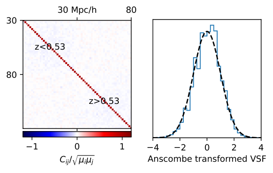
As a final point of this section, we substantiate the previous claim that the VSF is very close to Poissonian distributed. While this seems to be a natural assumption, void exclusion makes it non-trivial. Indeed, previous works have assumed Poisson likelihoods Sahlén 2019; Contarini et al. 2022a; our simulations enable us to check this assumption.
In Fig. 11, we show two checks performed with our fiducial mocks. The left panel shows the covariance matrix divided by the outer square of Poissonian standard deviations; the result is close to the identity. The right panel shows a check using the variance-stabilizing Anscombe transform Anscombe 1948. For each mock data vector and bin , we compute the transformed VSF count
| (4) |
In the limit of large counts the distribution of these transformed counts converges to the standard normal if the counts themselves are Poissonian. As can be seen, the agreement with the standard normal is quite good indeed. These tests demonstrate that deviations from Poissonian distribution are small for the VSF, at least for the choice of binning considered here.
V Conclusions
We have performed inference on galaxy clustering in the BOSS CMASS northern sample, combining the void size function, the void-galaxy cross power spectrum, and the galaxy auto power spectrum. Our primary target was the neutrino mass sum, ; thus, we imposed a tight prior on CDM informed by primary CMB data.
We argued that analytic models for the considered void statistics are not mature enough and unsuitable for our specific problem, necessitating a simulation-based approach. To this end, we ran approximate gravity-only simulations and populated them with galaxies using an expressive halo occupation distribution. Several factors motivated the use of implicit likelihood inference.
In our baseline analysis, we find from the galaxy auto power spectrum alone, and with the void statistics included ( credible interval). We performed several tests to confirm statistical and systematic validity of our likelihood approximation.
We performed a short investigation of the impact of voids on the neutrino mass posterior. It appears that the void statistics may be most effective in constraining from below. This result would imply that future analyses aiming at measuring may benefit from including void statistics.
Our results suggest that larger voids with effective radii carry most of the signal despite their lower abundance. This has interesting implications for future analyses, since voids of this size should be detectable in photometric catalogs with relatively low redshift error, such as the one expected for Rubin/LSST Ivezić et al. 2019. Of course, spectroscopic surveys such as DESI Dey et al. 2019, Euclid Laureijs et al. 2011, SPHEREx Doré et al. 2014, PFS Takada et al. 2014, and Roman Spergel et al. 2015 will continue to be cornerstones of void science. The trade-off between volume, galaxy number density, and redshift precision warrants further investigation.
We also demonstrate that the void size function is very close to Poisson distributed, a feature that had been assumed in previous analyses but never explicitly confirmed.
Future work could improve upon our analysis in multiple ways. First, the cosmo-varied simulations should be run with different random seeds (we decided for a fixed seed in anticipation of an emulator-based analysis which ultimately turned out to be very difficult). Second, it may be beneficial to normalize the void-galaxy cross power spectrum by void number. Although in principle this would contain the same information as our data vector once the VSF is included, the necessary transformation is non-linear and thus potentially invisible to our data compression. Third, the HOD modeling could be improved. Some of our priors may not be optimal, and our downsampling is simplistic. The CMASS sample’s completeness is quite well known and could be used to put a prior on the downsampling. Fourth, it turns out that the cosmological simulations did not dominate compute cost. It may therefore be economical to increase accuracy in FastPM or switch to a different solver.
Our results point toward a complicated picture with regard to the relationship between massive neutrinos and voids. Future data sets, both spectroscopic as well as photometric, promise to bring tight cosmological constraints from void science, since it scales well with number.
Acknowledgements.
We thank Sofia Contarini, Adrian Bayer, Jia Liu, Jo Dunkley, Masahiro Takada for useful discussions. We thank Oliver Philcox for explaining the EFTofLSS likelihood. The work of LT is supported by the NSF grant AST 2108078. The authors are pleased to acknowledge that the work reported on in this paper was substantially performed using the Princeton Research Computing resources at Princeton University which is a consortium of groups led by the Princeton Institute for Computational Science and Engineering (PICSciE) and Office of Information Technology’s Research Computing.Appendix A Halo occupation distribution
In this appendix, we provide a more detailed description of the adopted HOD model.
First, for reference, the baseline five-parameter model only depends on halo mass and has mean occupations
| (5) |
for the central galaxy and
| (6) |
for the satellites. A central is placed with probability and the number of satellites is drawn from a Poisson distribution with mean . The central is placed at the halo’s center and assigned the halo velocity. The satellites are distributed isotropically with an NFW profile Navarro et al. 1997 and the concentration model of Ref. Duffy et al. 2008, using the analytic solution for the inverse NFW CDF from Ref. Robotham and Howlett 2018. Satellite velocities are drawn from a distribution assuming virialization.
On top of this baseline model, we implement assembly bias using the decorated HOD Hearin et al. 2016a; Hearin et al. 2016b with the ratio of kinetic to potential energy as proxy for assembly history. In our preliminary tests outperformed halo concentration, possibly due to limited resolution within the FastPM halos. The decoration works by splitting halos into two groups according to . In order to reduce the effect of any potential evolution of with halo mass, we do this splitting separately within groups containing equal numbers of halos. The fraction of halos with lowest is assigned type 1 (2) for positive (negative) , while the rest is assigned type 2 (1). Then, the mean occupations are modified as
| (7) | ||||
| (8) |
for type 1 and
| (9) | ||||
| (10) |
for type 2.
Velocity bias for the centrals is implemented by adding where . For the satellites, the velocity difference from the host halo is scaled by .
Redshift dependence for , is approximated as linear in scale factor, such that
| (11) |
with .
We adopt flat priors , , , , , , , , , . Here, all masses are in , and the primed parameters are defined as , , . The above intervals were found during preliminary inference runs. Note in particular the small values of , compared to other analyses. This is partly explained by systematically lower halo masses in FastPM, and partly by the downsampling described below. We picked the transformations given by the primed parameters based on the intuition that strictly (mathematically) bounded intervals often indicate that a uniform prior in a transformed quantity is a better choice.
Appendix B Broadening of posteriors
We have seen in our main posteriors that adding void statistics to the data vector sometimes broadens the posterior on . In this appendix, we attempt to better understand this observation, focusing on . For this, we will rely on inference on our fiducial mocks.
The first possible explanation could be a statistical fluctuation, and we cannot definitely exclude this hypothesis. One way, however, to test it is to look at average posteriors on our fiducial mocks. We perform inference on randomly chosen mocks and plot the CDFs of concatenated chains in Fig. 12. There, we observe that the expected, average behavior is for the posterior to broaden once void statistics are added to the data vector.
The second possible explanation could be that once void statistics are added our compression procedure becomes less efficient. This could certainly be the case if at linear order the void statistics appear more constraining than they are globally, thus would be unnecessarily downweighted. This hypothesis appears unlikely in light of the full posteriors presented in Figs. 15, 16. In these posteriors, we observe that for the parameters that are actually constrained (like ) adding void statistics generically tightens the posteriors. It appears unlikely that should be an exception.
Having found these two hypotheses unsatisfactory, we arrive at the third one: void statistics tend to constrain from below. We illustrate this theory qualitatively in Fig. 13, which should not be interpreted as a literal depiction. In fact, in Sec. IV.4 we show that void statistics alone yield posteriors close to the prior. Fig. 13 provides merely an effective depiction.
We can investigate this hypothesis further by performing the following test. In order to increase signal-to-noise, we perform inference on four fiducial mocks at the same time, shown in Fig. 14. For this, we use a different set of neural nets in which we leave five nuisance parameters explicit. The reason is that all implicitly marginalized nuisance parameters are effectively assumed to be different for each of the four mocks, an effect we would like to minimize. Of course, increasing the number of explicit nuisance parameters complicates the training and we have less confidence in the precise calibration of the posteriors. For this reason, our baseline results were obtained with only two explicit nuisance parameters. For reference, the real data posteriors obtained with these alternative neural nets are shown in Fig. 16. We perform this test with two different sets of nuisance parameters kept explicit in order to gauge robustness (corresponding to the solid and dashed lines in Fig. 14). Similar to Fig. 12, we average posteriors over randomly chosen groups of four mocks in order to decrease sample variance. We observe that, consistent with our theory, the posteriors that include void statistics show a more pronounced hint of a bump at the true . In principle, one could increase the simulated volume further by combining more mocks, but our neural nets are not calibrated at the required level of precision and thus the resulting posteriors would not be robust.
In summary, the more mundane ideas to explain the observed broadening of posteriors appear questionable given the tests presented. On the other hand, the idea that void statistics are most effective at constraining from below receives support from our experiments. A more in-depth examination of this issue would constitute a great starting point for future work.
Appendix C Corner plots
This appendix collects posteriors in the full parameter spaces considered. Fig. 15 shows the baseline parameter space with two explicit nuisance parameters. Fig. 16 shows larger sections of parameter space (it should be mentioned, however, that the corresponding neural networks were trained without further hyperparameter optimization, implying a somewhat lower level of confidence in the validity of these posteriors). Fig. 17 shows our EFTofLSS posteriors, demonstrating that the CDM part of the parameter space is prior-dominated.
Appendix D Simulation budget
One might worry that the 127 cosmo-varied simulations are not enough to properly sample the cosmological prior. We test this by discarding a third of the simulations and training on the rest. The resulting posterior, compared to our baseline result, is shown in Fig. 18. Agreement between the two posteriors is almost perfect, demonstrating that our simulations cover the cosmological prior sufficiently well.
Appendix E Simulation data
About 50TB of halo catalogs, light cones, void catalogs, and summary statistics have been saved (at 20 times between and in 127 different massive-neutrino cosmologies with various HODs and 69 different initial conditions with a fiducial model). We are currently finalizing how to make this data set publicly available.
Appendix F Code
In terms of new code, we have written C++ code to populate halo catalogs with galaxies and to generate light cones including survey realism.
We have also written a C implementation of the quasi-random sampling scheme for uniform and Gaussian priors.
This work necessitated several small modifications to public codes:
- •
REPS: read files generated by the current CLASS version; write output in a user-defined directory.
- •
FastPM: do not write neutrinos to disk.
- •
bigfile: support for half-precision floats.
- •
Rockstar: native reading of the bigfile snapshots generated by FastPM (using the file chunking to read in distributed fashion since Rockstar does not use MPI).
- •
Rockstar/find_parents: output to bigfile with lower priority fields in half precision.
- •
cuboidremap: support for velocities.
- •
sbi: custom splitting into training and validation data.
Since all these items are relatively obscure, we do not provide documentation. However, we are happy to share any of these with interested researchers. A repository with most of the code is available at https://github.com/leanderthiele/nuvoid_production.
References
- Bahcall and Davis, Jr. (1976) J. N. Bahcall and R. Davis, Jr., Science 191, 264 (1976).
- Wolfenstein (1978) L. Wolfenstein, Phys. Rev. D 17, 2369 (1978).
- Mikheyev and Smirnov (1985) S. P. Mikheyev and A. Y. Smirnov, Yadernaya Fizika 42, 1441 (1985).
- Super-Kamiokande Collaboration et al. (1998) Super-Kamiokande Collaboration, Y. Fukuda, et al., Phys. Rev. Lett. 81, 1562 (1998), arXiv:hep-ex/9807003 [hep-ex] .
- SNO Collaboration et al. (2002) SNO Collaboration, Q. R. Ahmad, et al., Phys. Rev. Lett. 89, 011301 (2002), arXiv:nucl-ex/0204008 [nucl-ex] .
- KamLAND Collaboration et al. (2005) KamLAND Collaboration, T. Araki, et al., Phys. Rev. Lett. 94, 081801 (2005), arXiv:hep-ex/0406035 [hep-ex] .
- K2K Collaboration et al. (2006) K2K Collaboration, M. H. Ahn, et al., Phys. Rev. D 74, 072003 (2006), arXiv:hep-ex/0606032 [hep-ex] .
- Daya Bay Collaboration et al. (2012) Daya Bay Collaboration, F. P. An, et al., Phys. Rev. Lett. 108, 171803 (2012), arXiv:1203.1669 [hep-ex] .
- KATRIN Collaboration et al. (2022) KATRIN Collaboration, M. Aker, et al., Journal of Physics G Nuclear Physics 49, 100501 (2022), arXiv:2203.08059 [nucl-ex] .
- Planck Collaboration et al. (2020) Planck Collaboration, N. Aghanim, et al., Astron. Astrophys. 641, A6 (2020), arXiv:1807.06209 [astro-ph.CO] .
- Icke (1984) V. Icke, Mon. Not. Roy. Astron. Soc. 206, 1P (1984).
- Pisani et al. (2019) A. Pisani, E. Massara, D. N. Spergel, et al., Bull. Am. Astron. Soc. 51, 40 (2019), arXiv:1903.05161 [astro-ph.CO] .
- Moresco et al. (2022) M. Moresco et al., Living Reviews in Relativity 25, 6 (2022), arXiv:2201.07241 [astro-ph.CO] .
- Schuster et al. (2023) N. Schuster, N. Hamaus, K. Dolag, and J. Weller, J. Cosmol. Astropart. Phys. 2023, 031 (2023), arXiv:2210.02457 [astro-ph.CO] .
- Massara et al. (2015) E. Massara, F. Villaescusa-Navarro, M. Viel, and P. M. Sutter, J. Cosmol. Astropart. Phys. 2015, 018 (2015), arXiv:1506.03088 [astro-ph.CO] .
- Banerjee and Dalal (2016) A. Banerjee and N. Dalal, J. Cosmol. Astropart. Phys. 2016, 015 (2016), arXiv:1606.06167 [astro-ph.CO] .
- Kreisch et al. (2019) C. D. Kreisch, A. Pisani, C. Carbone, J. Liu, A. J. Hawken, E. Massara, D. N. Spergel, and B. D. Wandelt, Mon. Not. Roy. Astron. Soc. 488, 4413 (2019), arXiv:1808.07464 [astro-ph.CO] .
- Schuster et al. (2019) N. Schuster, N. Hamaus, A. Pisani, C. Carbone, C. D. Kreisch, G. Pollina, and J. Weller, J. Cosmol. Astropart. Phys. 2019, 055 (2019), arXiv:1905.00436 [astro-ph.CO] .
- Contarini et al. (2021) S. Contarini, F. Marulli, L. Moscardini, A. Veropalumbo, C. Giocoli, and M. Baldi, Mon. Not. Roy. Astron. Soc. 504, 5021 (2021), arXiv:2009.03309 [astro-ph.CO] .
- Verza et al. (2022) G. Verza, C. Carbone, A. Pisani, and A. Renzi, arXiv e-prints , arXiv:2212.09740 (2022), arXiv:2212.09740 [astro-ph.CO] .
- Sahlén (2019) M. Sahlén, Phys. Rev. D 99, 063525 (2019), arXiv:1807.02470 [astro-ph.CO] .
- Bayer et al. (2021a) A. E. Bayer, F. Villaescusa-Navarro, E. Massara, J. Liu, D. N. Spergel, L. Verde, B. D. Wandelt, M. Viel, and S. Ho, Astrophys. J. 919, 24 (2021a), arXiv:2102.05049 [astro-ph.CO] .
- Kreisch et al. (2022) C. D. Kreisch, A. Pisani, F. Villaescusa-Navarro, D. N. Spergel, B. D. Wandelt, N. Hamaus, and A. E. Bayer, Astrophys. J. 935, 100 (2022), arXiv:2107.02304 [astro-ph.CO] .
- Hotinli et al. (2023) S. C. Hotinli, N. Sabti, J. North, and M. Kamionkowski, arXiv e-prints , arXiv:2306.15715 (2023), arXiv:2306.15715 [astro-ph.CO] .
- Gregory and Thompson (1978) S. A. Gregory and L. A. Thompson, Astrophys. J. 222, 784 (1978).
- Jõeveer et al. (1978) M. Jõeveer, J. Einasto, and E. Tago, Mon. Not. Roy. Astron. Soc. 185, 357 (1978).
- Tully and Fisher (1978) R. B. Tully and J. R. Fisher, in Large Scale Structures in the Universe, Vol. 79, edited by M. S. Longair and J. Einasto (1978) p. 31.
- Kirshner et al. (1981) R. P. Kirshner, J. Oemler, A., P. L. Schechter, and S. A. Shectman, Astrophys. J. Lett. 248, L57 (1981).
- de Lapparent et al. (1986) V. de Lapparent, M. J. Geller, and J. P. Huchra, Astrophys. J. Lett. 302, L1 (1986).
- Sahlén et al. (2016) M. Sahlén, Í. Zubeldía, and J. Silk, Astrophys. J. Lett. 820, L7 (2016), arXiv:1511.04075 [astro-ph.CO] .
- Hoyle and Vogeley (2004) F. Hoyle and M. S. Vogeley, Astrophys. J. 607, 751 (2004), arXiv:astro-ph/0312533 [astro-ph] .
- Pan et al. (2012) D. C. Pan, M. S. Vogeley, F. Hoyle, Y.-Y. Choi, and C. Park, Mon. Not. Roy. Astron. Soc. 421, 926 (2012), arXiv:1103.4156 [astro-ph.CO] .
- Sutter et al. (2012a) P. M. Sutter, G. Lavaux, B. D. Wandelt, and D. H. Weinberg, Astrophys. J. 761, 44 (2012a), arXiv:1207.2524 [astro-ph.CO] .
- Sutter et al. (2014a) P. M. Sutter, G. Lavaux, B. D. Wandelt, D. H. Weinberg, M. S. Warren, and A. Pisani, Mon. Not. Roy. Astron. Soc. 442, 3127 (2014a), arXiv:1310.7155 [astro-ph.CO] .
- Nadathur (2016) S. Nadathur, Mon. Not. Roy. Astron. Soc. 461, 358 (2016), arXiv:1602.04752 [astro-ph.CO] .
- Mao et al. (2017a) Q. Mao, A. A. Berlind, R. J. Scherrer, M. C. Neyrinck, R. Scoccimarro, J. L. Tinker, C. K. McBride, D. P. Schneider, K. Pan, D. Bizyaev, E. Malanushenko, and V. Malanushenko, Astrophys. J. 835, 161 (2017a), arXiv:1602.02771 [astro-ph.CO] .
- Sutter et al. (2012b) P. M. Sutter, G. Lavaux, B. D. Wandelt, and D. H. Weinberg, Astrophys. J. 761, 187 (2012b), arXiv:1208.1058 [astro-ph.CO] .
- Sutter et al. (2014b) P. M. Sutter, A. Pisani, B. D. Wandelt, and D. H. Weinberg, Mon. Not. Roy. Astron. Soc. 443, 2983 (2014b), arXiv:1404.5618 [astro-ph.CO] .
- Hamaus et al. (2016) N. Hamaus, A. Pisani, P. M. Sutter, G. Lavaux, S. Escoffier, B. D. Wandelt, and J. Weller, Phys. Rev. Lett. 117, 091302 (2016), arXiv:1602.01784 [astro-ph.CO] .
- Hamaus et al. (2017) N. Hamaus, M.-C. Cousinou, A. Pisani, M. Aubert, S. Escoffier, and J. Weller, J. Cosmol. Astropart. Phys. 2017, 014 (2017), arXiv:1705.05328 [astro-ph.CO] .
- Mao et al. (2017b) Q. Mao, A. A. Berlind, R. J. Scherrer, M. C. Neyrinck, R. Scoccimarro, J. L. Tinker, C. K. McBride, and D. P. Schneider, Astrophys. J. 835, 160 (2017b), arXiv:1602.06306 [astro-ph.CO] .
- Hamaus et al. (2020) N. Hamaus, A. Pisani, J.-A. Choi, G. Lavaux, B. D. Wandelt, and J. Weller, J. Cosmol. Astropart. Phys. 2020, 023 (2020), arXiv:2007.07895 [astro-ph.CO] .
- Nadathur et al. (2020) S. Nadathur, A. Woodfinden, W. J. Percival, et al., Mon. Not. Roy. Astron. Soc. 499, 4140 (2020), arXiv:2008.06060 [astro-ph.CO] .
- Aubert et al. (2022) M. Aubert, M.-C. Cousinou, S. Escoffier, A. J. Hawken, S. Nadathur, et al., Mon. Not. Roy. Astron. Soc. 513, 186 (2022), arXiv:2007.09013 [astro-ph.CO] .
- Woodfinden et al. (2023) A. Woodfinden, W. J. Percival, S. Nadathur, H. A. Winther, T. S. Fraser, E. Massara, E. Paillas, and S. Radinovic, Mon. Not. Roy. Astron. Soc. 10.1093/mnras/stad1725 (2023), arXiv:2303.06143 [astro-ph.CO] .
- Contarini et al. (2022a) S. Contarini, A. Pisani, N. Hamaus, F. Marulli, L. Moscardini, and M. Baldi, arXiv e-prints , arXiv:2212.03873 (2022a), arXiv:2212.03873 [astro-ph.CO] .
- Contarini et al. (2022b) S. Contarini, A. Pisani, N. Hamaus, F. Marulli, L. Moscardini, and M. Baldi, arXiv e-prints , arXiv:2212.07438 (2022b), arXiv:2212.07438 [astro-ph.CO] .
- SDSS Collaboration et al. (2000) SDSS Collaboration, D. G. York, et al., Astron. J. 120, 1579 (2000), arXiv:astro-ph/0006396 [astro-ph] .
- SDSS Collaboration et al. (2011) SDSS Collaboration, D. J. Eisenstein, D. H. Weinberg, et al., Astron. J. 142, 72 (2011), arXiv:1101.1529 [astro-ph.IM] .
- SDSS Collaboration et al. (2013) SDSS Collaboration, K. S. Dawson, D. J. Schlegel, et al., Astron. J. 145, 10 (2013), arXiv:1208.0022 [astro-ph.CO] .
- Ivanov et al. (2020a) M. M. Ivanov, M. Simonović, and M. Zaldarriaga, Phys. Rev. D 101, 083504 (2020a), arXiv:1912.08208 [astro-ph.CO] .
- Semenaite et al. (2023) A. Semenaite, A. G. Sánchez, A. Pezzotta, J. Hou, A. Eggemeier, M. Crocce, C. Zhao, J. R. Brownstein, G. Rossi, and D. P. Schneider, Mon. Not. Roy. Astron. Soc. 521, 5013 (2023), arXiv:2210.07304 [astro-ph.CO] .
- Stopyra et al. (2021) S. Stopyra, H. V. Peiris, and A. Pontzen, Mon. Not. Roy. Astron. Soc. 500, 4173 (2021), arXiv:2007.14395 [astro-ph.CO] .
- Press and Schechter (1974) W. H. Press and P. Schechter, Astrophys. J. 187, 425 (1974).
- Bond et al. (1991) J. R. Bond, S. Cole, G. Efstathiou, and N. Kaiser, Astrophys. J. 379, 440 (1991).
- Sheth and Tormen (1999) R. K. Sheth and G. Tormen, Mon. Not. Roy. Astron. Soc. 308, 119 (1999), arXiv:astro-ph/9901122 [astro-ph] .
- Sheth and van de Weygaert (2004) R. K. Sheth and R. van de Weygaert, Mon. Not. Roy. Astron. Soc. 350, 517 (2004), arXiv:astro-ph/0311260 [astro-ph] .
- Paranjape et al. (2012) A. Paranjape, T. Y. Lam, and R. K. Sheth, Mon. Not. Roy. Astron. Soc. 420, 1429 (2012), arXiv:1105.1990 [astro-ph.CO] .
- Paranjape et al. (2013) A. Paranjape, R. K. Sheth, and V. Desjacques, Mon. Not. Roy. Astron. Soc. 431, 1503 (2013), arXiv:1210.1483 [astro-ph.CO] .
- Jennings et al. (2013) E. Jennings, Y. Li, and W. Hu, Mon. Not. Roy. Astron. Soc. 434, 2167 (2013), arXiv:1304.6087 [astro-ph.CO] .
- Pisani et al. (2015a) A. Pisani, P. M. Sutter, N. Hamaus, E. Alizadeh, R. Biswas, B. D. Wandelt, and C. M. Hirata, Phys. Rev. D 92, 083531 (2015a), arXiv:1503.07690 [astro-ph.CO] .
- Ronconi and Marulli (2017) T. Ronconi and F. Marulli, Astron. Astrophys. 607, A24 (2017), arXiv:1703.07848 [astro-ph.CO] .
- Ronconi et al. (2019) T. Ronconi, S. Contarini, F. Marulli, M. Baldi, and L. Moscardini, Mon. Not. Roy. Astron. Soc. 488, 5075 (2019), arXiv:1902.04585 [astro-ph.CO] .
- Verza et al. (2019) G. Verza, A. Pisani, C. Carbone, N. Hamaus, and L. Guzzo, J. Cosmol. Astropart. Phys. 2019, 040 (2019), arXiv:1906.00409 [astro-ph.CO] .
- Contarini et al. (2019) S. Contarini, T. Ronconi, F. Marulli, L. Moscardini, A. Veropalumbo, and M. Baldi, Mon. Not. Roy. Astron. Soc. 488, 3526 (2019), arXiv:1904.01022 [astro-ph.CO] .
- Contarini et al. (2022c) S. Contarini, G. Verza, A. Pisani, N. Hamaus, M. Sahlén, et al., Astron. Astrophys. 667, A162 (2022c), arXiv:2205.11525 [astro-ph.CO] .
- Pelliciari et al. (2023) D. Pelliciari, S. Contarini, F. Marulli, L. Moscardini, C. Giocoli, G. F. Lesci, and K. Dolag, Mon. Not. Roy. Astron. Soc. 522, 152 (2023), arXiv:2210.07248 [astro-ph.CO] .
- Alcock and Paczynski (1979) C. Alcock and B. Paczynski, Nature (London) 281, 358 (1979).
- Lavaux and Wandelt (2012) G. Lavaux and B. D. Wandelt, Astrophys. J. 754, 109 (2012), arXiv:1110.0345 [astro-ph.CO] .
- Pisani et al. (2014) A. Pisani, G. Lavaux, P. M. Sutter, and B. D. Wandelt, Mon. Not. Roy. Astron. Soc. 443, 3238 (2014), arXiv:1306.3052 [astro-ph.CO] .
- Padilla et al. (2005) N. D. Padilla, L. Ceccarelli, and D. G. Lambas, Mon. Not. Roy. Astron. Soc. 363, 977 (2005), arXiv:astro-ph/0508297 [astro-ph] .
- Paz et al. (2013) D. Paz, M. Lares, L. Ceccarelli, N. Padilla, and D. G. Lambas, Mon. Not. Roy. Astron. Soc. 436, 3480 (2013), arXiv:1306.5799 [astro-ph.CO] .
- Hamaus et al. (2014a) N. Hamaus, P. M. Sutter, and B. D. Wandelt, arXiv e-prints , arXiv:1409.7621 (2014a), arXiv:1409.7621 [astro-ph.CO] .
- Hamaus et al. (2014b) N. Hamaus, P. M. Sutter, and B. D. Wandelt, Phys. Rev. Lett. 112, 251302 (2014b), arXiv:1403.5499 [astro-ph.CO] .
- Massara and Sheth (2018) E. Massara and R. K. Sheth, arXiv e-prints , arXiv:1811.03132 (2018), arXiv:1811.03132 [astro-ph.CO] .
- Feng et al. (2016) Y. Feng, M.-Y. Chu, U. Seljak, and P. McDonald, Mon. Not. Roy. Astron. Soc. 463, 2273 (2016), arXiv:1603.00476 [astro-ph.CO] .
- Bayer et al. (2021b) A. E. Bayer, A. Banerjee, and Y. Feng, J. Cosmol. Astropart. Phys. 2021, 016 (2021b), arXiv:2007.13394 [astro-ph.CO] .
- Berlind and Weinberg (2002) A. A. Berlind and D. H. Weinberg, Astrophys. J. 575, 587 (2002), arXiv:astro-ph/0109001 [astro-ph] .
- Cooray and Sheth (2002) A. Cooray and R. Sheth, Phys. Rep. 372, 1 (2002), arXiv:astro-ph/0206508 [astro-ph] .
- Wechsler and Tinker (2018) R. H. Wechsler and J. L. Tinker, Annu. Rev. Astron. Astrophys. 56, 435 (2018), arXiv:1804.03097 [astro-ph.GA] .
- Cranmer et al. (2020) K. Cranmer, J. Brehmer, and G. Louppe, Proceedings of the National Academy of Science 117, 30055 (2020), arXiv:1911.01429 [stat.ML] .
- Hahn et al. (2022) C. Hahn, M. Eickenberg, S. Ho, J. Hou, P. Lemos, E. Massara, C. Modi, A. Moradinezhad Dizgah, B. Régaldo-Saint Blancard, and M. M. Abidi, arXiv e-prints , arXiv:2211.00723 (2022), arXiv:2211.00723 [astro-ph.CO] .
- Hahn et al. (2023) C. Hahn, M. Eickenberg, S. Ho, J. Hou, P. Lemos, E. Massara, C. Modi, A. Moradinezhad Dizgah, B. Régaldo-Saint Blancard, and M. M. Abidi, J. Cosmol. Astropart. Phys. 2023, 010 (2023), arXiv:2211.00660 [astro-ph.CO] .
- Philcox and Ivanov (2022) O. H. E. Philcox and M. M. Ivanov, Phys. Rev. D 105, 043517 (2022), arXiv:2112.04515 [astro-ph.CO] .
- Lewis et al. (2000) A. Lewis, A. Challinor, and A. Lasenby, Astrophys. J. 538, 473 (2000), arXiv:astro-ph/9911177 [astro-ph] .
- Howlett et al. (2012) C. Howlett, A. Lewis, A. Hall, and A. Challinor, J. Cosmol. Astropart. Phys. 1204, 027 (2012), arXiv:1201.3654 [astro-ph.CO] .
- Blas et al. (2011) D. Blas, J. Lesgourgues, and T. Tram, J. Cosmol. Astropart. Phys. 2011, 034 (2011), arXiv:1104.2933 [astro-ph.CO] .
- Zennaro et al. (2016) M. Zennaro, J. Bel, F. Villaescusa-Navarro, C. Carbone, E. Sefusatti, and L. Guzzo, REPS: REscaled Power Spectra for initial conditions with massive neutrinos, Astrophysics Source Code Library, record ascl:1612.022 (2016), ascl:1612.022 .
- Zennaro et al. (2017) M. Zennaro, J. Bel, F. Villaescusa-Navarro, C. Carbone, E. Sefusatti, and L. Guzzo, Mon. Not. Roy. Astron. Soc. 466, 3244 (2017), arXiv:1605.05283 [astro-ph.CO] .
- Villaescusa-Navarro et al. (2020) F. Villaescusa-Navarro, C. Hahn, E. Massara, A. Banerjee, A. M. Delgado, et al., Astrophys. J. Suppl. 250, 2 (2020), arXiv:1909.05273 [astro-ph.CO] .
- Akiba et al. (2019) T. Akiba, S. Sano, T. Yanase, T. Ohta, and M. Koyama, arXiv e-prints , arXiv:1907.10902 (2019), arXiv:1907.10902 [cs.LG] .
- Behroozi et al. (2012) P. Behroozi, R. Wechsler, and H.-Y. Wu, Rockstar: Phase-space halo finder, Astrophysics Source Code Library, record ascl:1210.008 (2012), ascl:1210.008 .
- Behroozi et al. (2013) P. S. Behroozi, R. H. Wechsler, and H.-Y. Wu, Astrophys. J. 762, 109 (2013), arXiv:1110.4372 [astro-ph.CO] .
- Zheng et al. (2005) Z. Zheng, A. A. Berlind, D. H. Weinberg, A. J. Benson, C. M. Baugh, S. Cole, R. Davé, C. S. Frenk, N. Katz, and C. G. Lacey, Astrophys. J. 633, 791 (2005), arXiv:astro-ph/0408564 [astro-ph] .
- Zhu et al. (2006) G. Zhu, Z. Zheng, W. P. Lin, Y. P. Jing, X. Kang, and L. Gao, Astrophys. J. Lett. 639, L5 (2006), arXiv:astro-ph/0601120 [astro-ph] .
- Zentner et al. (2014) A. R. Zentner, A. P. Hearin, and F. C. van den Bosch, Mon. Not. Roy. Astron. Soc. 443, 3044 (2014), arXiv:1311.1818 [astro-ph.CO] .
- Pujol and Gaztañaga (2014) A. Pujol and E. Gaztañaga, Mon. Not. Roy. Astron. Soc. 442, 1930 (2014), arXiv:1306.5761 [astro-ph.CO] .
- Reid et al. (2014) B. A. Reid, H.-J. Seo, A. Leauthaud, J. L. Tinker, and M. White, Mon. Not. Roy. Astron. Soc. 444, 476 (2014), arXiv:1404.3742 [astro-ph.CO] .
- Lin et al. (2016) Y.-T. Lin, R. Mandelbaum, Y.-H. Huang, H.-J. Huang, N. Dalal, B. Diemer, H.-Y. Jian, and A. Kravtsov, Astrophys. J. 819, 119 (2016), arXiv:1504.07632 [astro-ph.GA] .
- Kobayashi et al. (2022) Y. Kobayashi, T. Nishimichi, M. Takada, and H. Miyatake, Phys. Rev. D 105, 083517 (2022), arXiv:2110.06969 [astro-ph.CO] .
- Berlind et al. (2003) A. A. Berlind, D. H. Weinberg, A. J. Benson, C. M. Baugh, S. Cole, R. Davé, C. S. Frenk, A. Jenkins, N. Katz, and C. G. Lacey, Astrophys. J. 593, 1 (2003), arXiv:astro-ph/0212357 [astro-ph] .
- Yoshikawa et al. (2003) K. Yoshikawa, Y. P. Jing, and G. Börner, Astrophys. J. 590, 654 (2003), arXiv:astro-ph/0303053 [astro-ph] .
- van den Bosch et al. (2005) F. C. van den Bosch, S. M. Weinmann, X. Yang, H. J. Mo, C. Li, and Y. P. Jing, Mon. Not. Roy. Astron. Soc. 361, 1203 (2005), arXiv:astro-ph/0502466 [astro-ph] .
- Guo et al. (2015) H. Guo, Z. Zheng, I. Zehavi, K. Dawson, R. A. Skibba, J. L. Tinker, D. H. Weinberg, M. White, and D. P. Schneider, Mon. Not. Roy. Astron. Soc. 446, 578 (2015), arXiv:1407.4811 [astro-ph.CO] .
- Zhai et al. (2023) Z. Zhai, J. L. Tinker, A. Banerjee, J. DeRose, H. Guo, Y.-Y. Mao, S. McLaughlin, K. Storey-Fisher, and R. H. Wechsler, Astrophys. J. 948, 99 (2023), arXiv:2203.08999 [astro-ph.CO] .
- Carlson and White (2010) J. Carlson and M. White, Astrophys. J. Suppl. 190, 311 (2010), arXiv:1003.3178 [astro-ph.CO] .
- Sutter et al. (2015) P. M. Sutter, G. Lavaux, N. Hamaus, A. Pisani, B. D. Wandelt, M. Warren, F. Villaescusa-Navarro, P. Zivick, Q. Mao, and B. B. Thompson, Astronomy and Computing 9, 1 (2015), arXiv:1406.1191 [astro-ph.CO] .
- Neyrinck (2008) M. C. Neyrinck, Mon. Not. Roy. Astron. Soc. 386, 2101 (2008), arXiv:0712.3049 [astro-ph] .
- Colberg et al. (2008) J. M. Colberg, F. Pearce, C. Foster, E. Platen, R. Brunino, et al., Mon. Not. Roy. Astron. Soc. 387, 933 (2008), arXiv:0803.0918 [astro-ph] .
- van de Weygaert and Schaap (2009) R. van de Weygaert and W. Schaap, in Data Analysis in Cosmology, Vol. 665, edited by V. J. Martínez, E. Saar, E. Martínez-González, and M. J. Pons-Bordería (2009) pp. 291–413.
- Cautun et al. (2018) M. Cautun, E. Paillas, Y.-C. Cai, S. Bose, J. Armijo, B. Li, and N. Padilla, Mon. Not. Roy. Astron. Soc. 476, 3195 (2018), arXiv:1710.01730 [astro-ph.CO] .
- Hand et al. (2018) N. Hand, Y. Feng, F. Beutler, Y. Li, C. Modi, U. Seljak, and Z. Slepian, Astron. J. 156, 160 (2018), arXiv:1712.05834 [astro-ph.IM] .
- Hand et al. (2019) N. Hand, Y. Feng, F. Beutler, Y. Li, C. Modi, U. Seljak, and Z. Slepian, nbodykit: Massively parallel, large-scale structure toolkit, Astrophysics Source Code Library, record ascl:1904.027 (2019), ascl:1904.027 .
- Feldman et al. (1994) H. A. Feldman, N. Kaiser, and J. A. Peacock, Astrophys. J. 426, 23 (1994), arXiv:astro-ph/9304022 [astro-ph] .
- Reid et al. (2016) B. Reid, S. Ho, N. Padmanabhan, W. J. Percival, J. Tinker, et al., Mon. Not. Roy. Astron. Soc. 455, 1553 (2016), arXiv:1509.06529 [astro-ph.CO] .
- Cousinou et al. (2019) M. C. Cousinou, A. Pisani, A. Tilquin, N. Hamaus, A. J. Hawken, and S. Escoffier, Astronomy and Computing 27, 53 (2019), arXiv:1805.07181 [astro-ph.CO] .
- Pisani et al. (2015b) A. Pisani, P. M. Sutter, and B. D. Wandelt, arXiv e-prints , arXiv:1506.07982 (2015b), arXiv:1506.07982 [astro-ph.CO] .
- Ivanov et al. (2020b) M. M. Ivanov, M. Simonović, and M. Zaldarriaga, J. Cosmol. Astropart. Phys. 2020, 042 (2020b), arXiv:1909.05277 [astro-ph.CO] .
- Cranmer et al. (2015) K. Cranmer, J. Pavez, and G. Louppe, arXiv e-prints , arXiv:1506.02169 (2015), arXiv:1506.02169 [stat.AP] .
- Hermans et al. (2019) J. Hermans, V. Begy, and G. Louppe, arXiv e-prints , arXiv:1903.04057 (2019), arXiv:1903.04057 [stat.ML] .
- Durkan et al. (2020) C. Durkan, I. Murray, and G. Papamakarios, arXiv e-prints , arXiv:2002.03712 (2020), arXiv:2002.03712 [stat.ML] .
- Delaunoy et al. (2022) A. Delaunoy, J. Hermans, F. Rozet, A. Wehenkel, and G. Louppe, arXiv e-prints , arXiv:2208.13624 (2022), arXiv:2208.13624 [stat.ML] .
- Miller et al. (2022) B. K. Miller, C. Weniger, and P. Forré, arXiv e-prints , arXiv:2210.06170 (2022), arXiv:2210.06170 [stat.ML] .
- Foreman-Mackey et al. (2013a) D. Foreman-Mackey, A. Conley, W. Meierjurgen Farr, D. W. Hogg, D. Lang, P. Marshall, A. Price-Whelan, J. Sanders, and J. Zuntz, emcee: The MCMC Hammer, Astrophysics Source Code Library, record ascl:1303.002 (2013a), ascl:1303.002 .
- Foreman-Mackey et al. (2013b) D. Foreman-Mackey, D. W. Hogg, D. Lang, and J. Goodman, Publ. Astron. Soc. Pac. 125, 306 (2013b), arXiv:1202.3665 [astro-ph.IM] .
- Tejero-Cantero et al. (2020) A. Tejero-Cantero, J. Boelts, M. Deistler, J.-M. Lueckmann, C. Durkan, P. J. Gonçalves, D. S. Greenberg, and J. H. Macke, Journal of Open Source Software 5, 2505 (2020).
- Heavens et al. (2000) A. F. Heavens, R. Jimenez, and O. Lahav, Mon. Not. Roy. Astron. Soc. 317, 965 (2000), arXiv:astro-ph/9911102 [astro-ph] .
- Alsing and Wandelt (2019) J. Alsing and B. Wandelt, Mon. Not. Roy. Astron. Soc. 488, 5093 (2019), arXiv:1903.01473 [astro-ph.CO] .
- d’Amico et al. (2020) G. d’Amico, J. Gleyzes, N. Kokron, K. Markovic, L. Senatore, P. Zhang, F. Beutler, and H. Gil-Marín, J. Cosmol. Astropart. Phys. 2020, 005 (2020), arXiv:1909.05271 [astro-ph.CO] .
- Chen et al. (2022) S.-F. Chen, Z. Vlah, and M. White, J. Cosmol. Astropart. Phys. 2022, 008 (2022), arXiv:2110.05530 [astro-ph.CO] .
- Philcox et al. (2020) O. H. E. Philcox, M. M. Ivanov, M. Simonović, and M. Zaldarriaga, J. Cosmol. Astropart. Phys. 2020, 032 (2020), arXiv:2002.04035 [astro-ph.CO] .
- Philcox (2021) O. H. E. Philcox, Phys. Rev. D 103, 103504 (2021), arXiv:2012.09389 [astro-ph.CO] .
- Chudaykin et al. (2020) A. Chudaykin, M. M. Ivanov, O. H. E. Philcox, and M. Simonović, Phys. Rev. D 102, 063533 (2020), arXiv:2004.10607 [astro-ph.CO] .
- Hermans et al. (2021) J. Hermans, A. Delaunoy, F. Rozet, A. Wehenkel, V. Begy, and G. Louppe, arXiv e-prints , arXiv:2110.06581 (2021), arXiv:2110.06581 [stat.ML] .
- Anscombe (1948) F. J. Anscombe, Biometrika 35, 246 (1948), https://academic.oup.com/biomet/article-pdf/35/3-4/246/785684/35-3-4-246.pdf .
- Ivezić et al. (2019) Ž. Ivezić, S. M. Kahn, J. A. Tyson, B. Abel, E. Acosta, et al., Astrophys. J. 873, 111 (2019), arXiv:0805.2366 [astro-ph] .
- Dey et al. (2019) A. Dey, D. J. Schlegel, D. Lang, et al., Astron. J. 157, 168 (2019), arXiv:1804.08657 [astro-ph.IM] .
- Laureijs et al. (2011) R. Laureijs, J. Amiaux, S. Arduini, J. L. Auguères, J. Brinchmann, R. Cole, et al., arXiv e-prints , arXiv:1110.3193 (2011), arXiv:1110.3193 [astro-ph.CO] .
- Doré et al. (2014) O. Doré, J. Bock, et al., arXiv e-prints , arXiv:1412.4872 (2014), arXiv:1412.4872 [astro-ph.CO] .
- Takada et al. (2014) M. Takada, R. S. Ellis, M. Chiba, J. E. Greene, H. Aihara, et al., Publ. Astron. Soc. Jpn. 66, R1 (2014), arXiv:1206.0737 [astro-ph.CO] .
- Spergel et al. (2015) D. Spergel, N. Gehrels, C. Baltay, D. Bennett, J. Breckinridge, et al., arXiv e-prints , arXiv:1503.03757 (2015), arXiv:1503.03757 [astro-ph.IM] .
- Navarro et al. (1997) J. F. Navarro, C. S. Frenk, and S. D. M. White, Astrophys. J. 490, 493 (1997), arXiv:astro-ph/9611107 [astro-ph] .
- Duffy et al. (2008) A. R. Duffy, J. Schaye, S. T. Kay, and C. Dalla Vecchia, Mon. Not. Roy. Astron. Soc. 390, L64 (2008), arXiv:0804.2486 [astro-ph] .
- Robotham and Howlett (2018) A. S. G. Robotham and C. Howlett, Research Notes of the American Astronomical Society 2, 55 (2018), arXiv:1805.09550 [astro-ph.CO] .
- Hearin et al. (2016a) A. P. Hearin, A. R. Zentner, F. C. van den Bosch, D. Campbell, and E. Tollerud, Mon. Not. Roy. Astron. Soc. 460, 2552 (2016a), arXiv:1512.03050 [astro-ph.CO] .
- Hearin et al. (2016b) A. Hearin, E. Tollerud, T. Robitaille, M. Droettboom, A. Zentner, et al., Halotools: Galaxy-Halo connection models, Astrophysics Source Code Library, record ascl:1604.005 (2016b), ascl:1604.005 .