Variational dynamics of open quantum systems in phase space
Abstract
We present a method to simulate the dynamics of large driven-dissipative many-body open quantum systems using a variational encoding of the Wigner or Husimi-Q quasi-probability distributions. The method relies on Monte-Carlo sampling to maintain a polynomial computational complexity while allowing for several quantities to be estimated efficiently. As a first application, we present a proof of principle investigation into the physics of the driven-dissipative Bose-Hubbard model with weak nonlinearity, providing evidence for the high efficiency of the phase space variational approach.
Introduction
The development of larger quantum devices for quantum technology applications is increasingly defying the efficiency of theoretical models and simulation methods used to design and validate such devices Bruzewicz et al. 2019; Cirac 2020; Kjaergaard et al. 2020; Browaeys and Lahaye 2020. These devices are open, namely subject to the influence of the surrounding environment, both as a nuisance and as a way of control, making it possible to develop quantum correlations and mixedness through the action of the environment, which can steer the dynamics of the system Rotter and Bird 2015; Koch 2016; Leghtas et al. 2015; de Neeve et al. 2022.
The mixed nature of the state describing an open quantum system arises by the tracing out of the environment degrees of freedom. This state is then usually encoded as a (positive semidefinite) density matrix. The dynamics can then be described by the Lindblad master equation (LME, eq. 1) under the assumption of a memoryless (i.e., Markovian) bath weakly interacting with the system such that its state remains unperturbed (Born approximation) Gardiner and Zoller 2000; Breuer and Petruccione 2007a. Three mainstream representations of such dynamics exist, all retrieving the same expectation values of any operator: the integration of the LME, the unraveling of the density matrix through stochastic wave functions called quantum trajectories, and the integration of the differential equations describing quasi-probability functions in phase space.
First, solving the LME for a quantum system, defined in a -dimensional Hilbert space, requires solving coupled linear ordinary differential equations (ODEs). Second, the unraveling of the master equation onto a statistical ensemble of stochastic quantum trajectories Mølmer et al. 1993; Breuer and Petruccione 2007b; Gardiner and Zoller 2000, requires solving coupled linear stochastic differential equations (SDEs) multiple times until statistical convergence is established. Both methods suffer the curse of dimensionality, as the number of differential equations to be solved scales exponentially with the number of modes, and calls for efficient numerical methods and approximations Weimer et al. 2021. These include mean-field Jin et al. 2016; Verstraelen and Wouters 2018; Verstraelen et al. 2023 and linked-cluster expansions Biella et al. 2018, and corner-space renormalization Finazzi et al. 2015; Donatella et al. 2021.
The third possibility is the description of an open quantum system in terms of a quasi-probability distribution (QPD) in phase space Carmichael 1999; Gardiner and Zoller 2000; Walls and Milburn 2008; Polkovnikov 2010; Rundle and Everitt 2021. Then, a QPD is governed by a partial differential equation (PDE) whose dimensionality is set by the number of modes composing the system. While QPDs are useful analytical tools, numerically integrating such partial differential equations with no further approximations is usually a much harder task than the original problem where fewer algorithms are available and most scale poorly as dimensionality increases. While some progress have been made in this direction Veronez and de Aguiar 2013; Holmes et al. 2023; Roda-Llordes et al. 2023, the presence of higher-order terms in the differential equation, and in the highly-singular nature of the solutions adds considerable challenges Drummond and Gardiner 1980; Walls and Milburn 2008; Gilchrist et al. 1997. Only in specific cases or approximations, where governing PDE reduces to true a Fokker-Planck equation, have phase space methods been extensively investigated and adopted to simulate a variety of (multi-mode) models of open and closed quantum systems Gilchrist et al. 1997; Deuar et al. 2021; Kiesewetter et al. 2014; Vogel and Risken 1989; Sinatra et al. 2002; Deuar and Drummond 2002; Plimak et al. 2003; Carusotto and Ciuti 2013; Foss-Feig et al. 2017; Vicentini et al. 2018; Huber et al. 2022. Indeed, such approximations are often limited to weakly-interacting, almost semi-classical systems.
Numerical methods that reduce the computational complexity of the problem and that can deal with strong interactions and non-classical states focused mainly on a discrete description of the LME, for example leveraging variational ansätze Weimer 2015; Overbeck et al. 2017, including tensor- Cui et al. 2015; Mascarenhas et al. 2015; Werner et al. 2016; Orús 2014; Weimer et al. 2021 or neural-network representations Nagy and Savona 2019; Hartmann and Carleo 2019; Vicentini et al. 2019; Yoshioka and Hamazaki 2019 of the quantum state. Recent works have refined the latter method, either by ensuring that the ansatz is always physical for arbitrary network depths Vicentini et al. 2022 or by leveraging more efficient, nonphysical parametrizations Reh et al. 2021; Luo et al. 2022.
However, generalizing such variational methods to the LME for bosonic systems in a truncated Fock space has proven challenging so far Saito 2017. To this day, an efficient and reliable approach to encoding the wave-function or density-matrix of an bosonic open system – or more generally of a system with a very large local Hilbert space dimension – on a neural network is not known. One-hot encodings of the local degree of freedom to find the ground state have been tested Saito and Kato 2018; Çeven et al. 2022, but their computational cost is high Pei and Clark 2021. For closed systems, an efficient representation of a bosonic system was found by using a first-quantized description of the wave-function in the position basis Saito 2018; Pescia et al. 2022, but the conservation of particle number cannot be directly translated to the dynamics of open systems.
Following this intuition, the phase space and its natural position-momentum variables emerges as a suitable platform to implement the variational principle for bosons or continuous variable systems. Indeed, the possibility of representing a true Fokker-Planck equation with variational ansätze has recently emerged Reh and Gärttner 2022. Very recently, the same idea has been applied to QPDs of coupled linear modes Dugan et al. 2023.
Here, we apply the time-dependent variational principle (tVMC) to parameterized phase space functions, and show that we can accurately simulate time evolution of driven-dissipative systems in the limit of small but nonvanishing nonlinearity, up to arbitrary occupation number. We apply the tVMC method using both a neural-network and a complex-Gaussian variational ansatz. We discuss the limitations of the adopted variational ansatz and of the size of the time step in the tVMC context. As the output of the model is the full QPD, quantum correlations among modes are efficiently described. Moreover, sampling the variational QPD allows for efficient calculation of expectation values of quantities such as occupation number, Wigner negativity and entropy. We show several proof-of-concept results involving Wigner negativity, non-Gaussian initial conditions, forcing, dissipation, and explore the limitations imposed by nonlinearity.
Results and discussion
Phase space representation
We consider a quantum system consisting of M bosonic modes dissipatively coupled to a Markovian environment. The dynamics is governed by the Lindblad master equation (LME) for the density matrix Breuer and Petruccione 2007a; Gardiner and Zoller 2000. Setting ,
| (1) |
where is the system Hamiltonian and denotes the Liouvillian superoperator which generates the non-unitary dynamics. The dissipator is defined in terms of the jump operators as . Phase space methods exactly map the state of the system on one of several possible quasi-probability distributions (QPDs) , and the dynamics equation (1) onto a PDE that determines the evolution of the QPD. The particular structure of the PDE is determined by the choice of QPD. The most relevant choices are the Wigner, Glauber P, and Husimi-Q distributions, for which the mapping are reviewed in the SI.
Many-body interactions and dissipation can lead to a high-order PDE describing the function . Most applications of phase space methods truncate terms higher than second order, thereby yielding a 2M dimensional quasi Fokker-Planck (FP) equation characterized by a drift vector and diffusion tensor Drummond and Hillery 2014; Gardiner and Zoller 2014:
| (2) | ||||
Here, for modes. Since it is not possible to numerically integrate eq. 2 with standard solution techniques such as finite element or finite difference methods beyond three dimensions Pichler et al. 2013; Dobson et al. 2019; Zhai et al. 2020, stochastic differential equation (SDE) trajectory methods are usually employed Carmichael 1999; Gardiner and Zoller 2000; Walls and Milburn 2008; Polkovnikov 2010; Gilchrist et al. 1997; Deuar et al. 2021; Kiesewetter et al. 2014; Vogel and Risken 1989; Sinatra et al. 2002; Deuar and Drummond 2002. However, to do so, the PDE must be a true FP equation, meaning that should be non-negative, and the diffusion matrix should be positive-semi-definite. These two requirements respectively rule out the negative Wigner function and the Husimi-Q function. In addition, when long-range quantum correlations dominate over local dissipation, the number of trajectories to sample the QPD may grow exponentially and the SDEs become unstable Deuar et al. 2021.
Variational ansatz and tVMC
Instead, in the following examples, we use a variational approach to integrate eq. 2, where the drift and diffusion operators depend on the parameters of the Hamiltonian, the dissipator, and the chosen QPD (Sec. Methods details the procedure to construct eq. 2, and gives an example of a specific form in eq. 15). We follow a scheme similar to variational neural-network quantum states, which have been successfully used to compress the wave-function of quantum systems with discrete Carleo and Troyer 2017; Chen and Heyl 2023 or continuous degrees of freedom Saito 2018; Pescia et al. 2022; Lovato et al. 2022 onto a polynomially-large set of variational parameters .
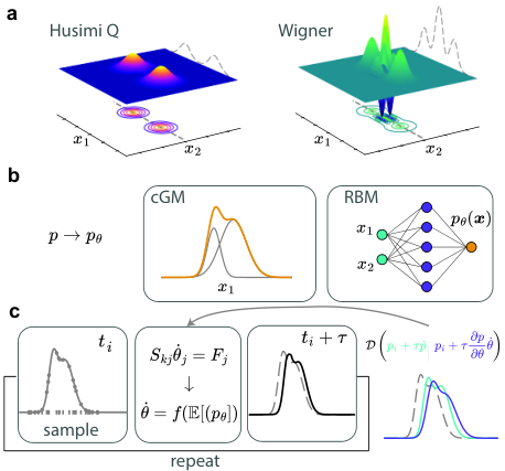
In particular, we efficiently represent the logarithm of the Husimi-Q () or Wigner () QPD with a variational function which may in general not be normalized (fig. 1(a)). The time-dependence is encoded in the parameters , which are in a 1-to-1 correspondence with quantum states. The details of the variational function are given in Sec. Methods. We explore two ansätze: a complex Gaussian mixture (cGM) and a restricted Boltzmann machine (RBM) (fig. 1(b)). We approximately map the PDE onto a system of ODEs for by means of two variational principles for the and QPDs Yuan et al. 2019; Reh and Gärttner 2022. In both cases, we obtain the differential equation
| (3) |
where the entries of the vector of so-called variational forces and the quantum geometric tensor are defined as
| (4) | ||||
| (5) |
(We drop the dependency of from the parameters to lighten the notation.)
To derive this equation, we minimize the distance between the time evolution of the QPD and the parameter evolution ,
| (6) |
It is essential to chose a distance that leads to quantities that can be (i) estimated by sampling an expectation value, and (ii) have finite variance. In particular, the Kullback–Leibler or Hellinger distance is a valid choice for the Husimi-Q Reh and Gärttner 2022 as it is positive and we can directly sample it (). For the Wigner QPD, instead, we select the norm because it can be efficiently estimated by sampling () 11 1 This is strictly equivalent to re-deriving the McLachlan variational principle Yuan et al. 2019 for the QPD.
We then replace the integrals in eqs. 4 and 5 with unbiased stochastic estimates that require sampling the QPD or some power of it Carleo et al. 2017; Schmitt and Heyl 2020; Reh et al. 2021 (fig. 1(c)). We remark that this approach is conceptually different from what is known as Physics-Informed Neural Networks (PINNs), where a variational ansatz is taken to represent the state at all points in space and time and the continuity equation is enforced on a randomly sampled grid Chen et al. 2018; Cai et al. 2021a; Cai et al. 2021b.
Single-mode benchmark

We first consider a system of one anharmonic oscillator governed by the Hamiltonian
| (7) |
and dissipator . Here is the bosonic annihilation operator, obeying , and are respectively the bare energy and anharmonic strength of the oscillator, and is the dissipation rate. In what follows, we take and and assume an initial Schrödinger cat state . We simulate the dynamics using a cGM ansatz with Gaussian components. Snapshots of the Wigner and Husimi-Q functions are shown in Figure 2 (a-c) and (e-g) respectively. We numerically show that our variational approach can describe the departure from the cat state, originating from the anharmonic effects. The accuracy of the simulation is assessed by comparing against a numerically exact solution of the Lindblad master equation Johansson et al. 2013. Figure 2(d) and (h) respectively show the mean squared error and a fidelity defined as in terms of the Hellinger distance . Based on these metrics, the variational Husimi-Q function represents the state of the system almost exactly, while the truncated Wigner approximation departs slightly from the exact solution due to the anharmonic terms that are approximated by the truncation.
To prove the predictive value of our method, we also show that we can cheaply estimate quantities such as the Wehrl entropy by using Monte-Carlo integration, which are otherwise computationally intractable for trajectory methods. The Wehrl entropy Wehrl 1979 for the Husimi-Q function is defined as
| (8) |
where the last identity shows how it can be naturally estimated by sampling the QPD. The quantity , plotted in fig. 2(h), decreases along the dynamics, as expected for a purely dissipative system.
For the Wigner function, the negative volume is defined as , where if Pizzimenti et al. 2023. The quantity , shown in fig. 2(h), vanishes as the cat state decays to the vacuum.

We now consider a driven-dissipative system with Hamiltonian
| (9) |
and the same dissipator as before. This description of a Kerr resonator is a hallmark example in quantum optics Vogel and Risken 1989; Gardiner and Zoller 2000. Here, is the (real) driving field amplitude, and the Hamiltonian is expressed in the rotating frame of the drive, so that represents the frequency detuning between the mode and the driving field. For this case, we set the initial state to be an arbitrary mixed state. Specifically, we choose a state in the bistability region of parameters of the Kerr-resonator Vogel and Risken 1989; Drummond and Gardiner 1980. The initial state is chosen so as to differ from the steady state for the given system parameters. The results are displayed in fig. 3. Both ansätze accurately describe the non-Gaussian pattern in the QPD arising along the dynamics, as seen in the time snapshots of fig. 3(a,b). In fig. 3(c), the fidelity computed along the dynamics is displayed, showing that both the RBM and the cGM ansätze efficiently represent the QPD dynamics.
Several coupled modes
Simulating the dynamics of several coupled modes provides evidence for the efficiency of the method. We first perform simulations on coupled modes – a system that can still be reasonably simulated by direct integration of the Lindblad master equation on a truncated Fock space. The system is characterized by the Hamiltonian
| (10) | ||||
The modes are coupled through nearest neighbor hopping with periodic boundary conditions. Here, is the coupling constant, is the strength of the Kerr nonlinearity, is the frequency detuning of the driving field, and is the driving field strength. All modes are coupled to the environment through the dissipator . We assume that only the first mode is driven with . The system is initialized to a coherent state in each mode, with values , and . While our method gives the evolution of the full continuous 6 dimensional Husimi-Q function, expectation values of physical observables can again be efficiently obtained through sampling.
Figure 4 shows the evolution the real and imaginary parts of the field expectation values , with . The RBM and the cGM ansatz closely follow the direct integration of the LME. The same quantities for are also displayed in Figure 4, showing the strong influence of the nonlinearity on the evolution.
We now consider a higher number of coupled modes, for which the direct solution of the LME is no longer feasible with reasonable computational means. To assess the accuracy of the phase space tVMC method, we compare the results to those obtained via truncated cumulant expansion Kubo 1962; Plankensteiner et al. 2022. Figure 4(c,d) shows the dynamics of the field expectation values for coupled modes governed by the Hamiltonian eq. 10. The initial state is again set to a tensor product of coherent states, with values . For , the simulation using an RBM ansatz closely follows the exact result of the first order cumulant expansion or Gross-Pitavskii equation. For a finite nonlinearity , the accuracy of the variational phase space method is confirmed by solving for two different time steps and , and comparing to the second order cumulant expansion.
Influence of nonlinearity.
In order to assess the influence of nonlinear terms on the predictive power of the method, we study the simplest case of a single mode undergoing the competition of nonlinearity and dissipation (see SI for more details). We set an initial coherent state . As the nonlinear term induces a departure from a Gaussian pattern in phase space, we expect the cGM to become rapidly less expressive as is increased. The RBM ansatz is more flexible, but we still expect difficulties due to the Gaussian tail-behavior that we have assumed. Figure 5(a) shows the departure from a Gaussian shape as is increased, at a fixed propagation time .
A higher value of results in a lower fidelity, and eventually leads to a numerical instability of the solver, for both the RBM and the cGM. Increasing the number of parameters does not improve the performance. However, we observe that decreasing the time step drastically improves the performance.
Indeed, in presence of nonlinearity, the PDE eq. 2 becomes stiff and the first-order integration scheme used to treat integrate eq. 3 requires an increasingly small time-step to yield accurate results. We expect that higher-order, adaptive time-stepping scheme would mitigate the problems, yet, a straightforward application such as that discussed in Ref. Schmitt and Heyl 2020 does not help. Alternatively, recently proposed implicit integration schemes solving a non-convex optimisation problem at each time-step, which allow for non-smooth evolutions along the variational manifold, might be more stable Sinibaldi et al. 2023; Donatella et al. 2022; Gutiérrez and Mendl 2022.
Conclusions.
We have demonstrated that the dynamics of driven-dissipative open quantum systems made of several coupled bosonic modes can be efficiently integrated in phase space, by introducing a parameterized ansatz for the Wigner or Husimi-Q QPDs, and adopting the tVMC method for their evolution. In this way, and by choosing an appropriately expressive variational ansatz, the large dimensionality of the many-body problem can be drastically reduced. Specifically, we turn a high dimensional PDE into a set of ODE’s, at the cost of having to sample the the parameterized function. We provided empirical evidence that the variational phase space approach is particularly efficient in cases where the bosonic modes are characterized by a weak nonlinearity. We simulated the dynamics of several models with various initial conditions, giving a proof of principle of the efficiency of the variational phase space approach. An advantage of variationally representing the QPD in phase space is that some relevant observables, such as various entropy definitions, are easily accessible. Numerical simulations suggest that the main limitations of the present method are the representative power of the ansatz and the size of the time step, similarly to most tVMC approaches. In particular, these factors set an upper bound to the strength of nonlinearity that can be accommodated. The exploration of different, more complex ansätze, as well as the inclusion of an adaptive time step approach Sinibaldi et al. 2023 are therefore a prospect for future research. In addition, the question of whether derivatives beyond the second order in the PDE can be included remains open. Finally, the present approach could also be advantageous for other fields, besides quantum physics, where non-Gaussian high-dimensional Fokker-Planck equations are involved.
Methods
Mappings quasi-Fokker-Planck equation:
The mappings between operators in the Lindbland master equation eq. 1 and quasi-FP equation for eq. 2 , see e.g. Gardiner and Zoller 2014 are
| (11) | |||||||
| (12) | |||||||
| (13) | |||||||
| (14) |
These can be applied iteratively to obtain the correct terms. As an example, for eq. 7 in combination with the dissipator , this yields the following quasi-FP equation for the Husimi-Q QPD, separating the real and imaginary part
| (15) | ||||
with .
See SI for the remaining quasi-FP equations corresponding to the examples in the main text.
Details on the variational ansatz:
We explore two ansätze to parameterize , a complex Gaussian mixture (cGM) and a restricted Boltzmann machine (RBM) see fig. 1. The cGM consists of Gaussians , for , where is the relative weight or normalization of each Gaussian and , with complex mean and complex covariance matrix . Separating the real and imaginary part, the length of the parameter vector , . The Wigner and Q function of a cat state can be represented by the sum of four complex Gaussians (see the SI and Ref. Bourassa et al. 2021).
The RMB-based ansatz is defined as a tail-regularized 1-layer feed forward neural network: , with hidden nodes with hyperbolic tangent activation function. The coefficient enforces the correct tail behaviour. The parameters are ), where are the network weights and its biases, has length . The initial condition for the evolution can be obtained by either fitting the ansatz of choice by means of gradient descent techniques to the discretized QPD corresponding to a given density matrix, or to an analytic expression.
Monte-Carlo sampling
Quantum-mechanical observables and quantities needed to compute the variational dynamics are computed using Monte-Carlo sampling of the QPD in the spirit of variational Monte Carlo. If is a valid probability distribution, such as for the Husimi-Q QPD, we write quantum expectation values as
| (16) |
where is obtained from the mappings of operators to phase space (see Sec.A of the SI). We explicitly write the denominator because the distribution is generally not normalized to 1. The Wigner QPD, instead, can take on negative values and we cannot sample from it directly. Instead, we rewrite expectation values as statistical averages over samples drawn from as follows,
| (17) | ||||
These expectation values are then estimated by their sample mean over a polynomially-large set of samples obtained from a Markov-Chain Monte-Carlo sampling procedure (see Ref. Vicentini et al. 2021 for details of the MCMC implementation employed).
New configurations for the chains are generated by the gaussian transition rule
| (18) |
where is a normal distribution with mean and variance .
The operators, sampling procedure and time step can be conveniently be implemented using the continuous variable back-end of NetKet Vicentini et al. 2021, and utilizing its integrated parallelization options.
Code availability
The code used in this study is available from the authors on reasonable request.
References
- Bruzewicz et al. (2019) C. D. Bruzewicz, J. Chiaverini, R. McConnell, and J. M. Sage, Trapped-ion quantum computing: Progress and challenges, Applied Physics Reviews 6, 021314 (2019).
- Cirac (2020) J. I. Cirac, Quantum computing and simulation, Nanophotonics 10, 453 (2020).
- Kjaergaard et al. (2020) M. Kjaergaard, M. E. Schwartz, J. Braumüller, P. Krantz, J. I.-J. Wang, S. Gustavsson, and W. D. Oliver, Superconducting qubits: Current state of play, Annual Review of Condensed Matter Physics 11, 369 (2020).
- Browaeys and Lahaye (2020) A. Browaeys and T. Lahaye, Many-body physics with individually controlled rydberg atoms, Nature Physics 16, 132 (2020).
- Rotter and Bird (2015) I. Rotter and J. P. Bird, A review of progress in the physics of open quantum systems: Theory and experiment, Reports on Progress in Physics 78, 114001 (2015).
- Koch (2016) C. P. Koch, Controlling open quantum systems: Tools, achievements, and limitations, Journal of Physics: Condensed Matter 28, 213001 (2016).
- Leghtas et al. (2015) Z. Leghtas, S. Touzard, I. M. Pop, A. Kou, B. Vlastakis, A. Petrenko, K. M. Sliwa, A. Narla, S. Shankar, M. J. Hatridge, M. Reagor, L. Frunzio, R. J. Schoelkopf, M. Mirrahimi, and M. H. Devoret, Confining the state of light to a quantum manifold by engineered two-photon loss, Science 347, 853 (2015).
- de Neeve et al. (2022) B. de Neeve, T.-L. Nguyen, T. Behrle, and J. P. Home, Error correction of a logical grid state qubit by dissipative pumping, Nature Physics 18, 296 (2022).
- Gardiner and Zoller (2000) C. W. Gardiner and P. Zoller, Quantum Noise, 2nd ed., edited by H. Haken (Springer, 2000).
- Breuer and Petruccione (2007a) H.-P. Breuer and F. Petruccione, The Theory of Open Quantum Systems, 1st ed. (Oxford University PressOxford, 2007).
- Mølmer et al. (1993) K. Mølmer, Y. Castin, and J. Dalibard, Monte Carlo wave-function method in quantum optics, Josa B 10, 524 (1993).
- Breuer and Petruccione (2007b) H.-P. Breuer and F. Petruccione, The Theory of Open Quantum Systems (Oxford University Press, Oxford, New York, 2007).
- Weimer et al. (2021) H. Weimer, A. Kshetrimayum, and R. Orús, Simulation methods for open quantum many-body systems, Reviews of Modern Physics 93, 015008 (2021).
- Jin et al. (2016) J. Jin, A. Biella, O. Viyuela, L. Mazza, J. Keeling, R. Fazio, and D. Rossini, Cluster mean-field approach to the steady-state phase diagram of dissipative spin systems, Phys. Rev. X 6, 031011 (2016).
- Verstraelen and Wouters (2018) W. Verstraelen and M. Wouters, Gaussian quantum trajectories for the variational simulation of open quantum-optical systems, Applied Sciences 8, 1427 (2018).
- Verstraelen et al. (2023) W. Verstraelen, D. Huybrechts, T. Roscilde, and M. Wouters, Quantum and classical correlations in open quantum-spin lattices via truncated-cumulant trajectories, (2023), arXiv:2209.13377 [quant-ph] .
- Biella et al. (2018) A. Biella, J. Jin, O. Viyuela, C. Ciuti, R. Fazio, and D. Rossini, Linked cluster expansions for open quantum systems on a lattice, Phys. Rev. B 97, 035103 (2018).
- Finazzi et al. (2015) S. Finazzi, A. L. Boité, F. Storme, A. Baksic, and C. Ciuti, Corner-space renormalization method for driven-dissipative two-dimensional correlated systems, Physical Review Letters 115, 10.1103/physrevlett.115.080604 (2015).
- Donatella et al. (2021) K. Donatella, Z. Denis, A. Le Boité, and C. Ciuti, Continuous-time dynamics and error scaling of noisy highly entangling quantum circuits, Phys. Rev. A 104, 062407 (2021).
- Carmichael (1999) H. J. Carmichael, Statistical Methods in Quantum Optics 1 (Springer, Berlin, Heidelberg, 1999).
- Walls and Milburn (2008) D. Walls and G. J. Milburn, eds., Quantum Optics (Springer, Berlin, Heidelberg, 2008).
- Polkovnikov (2010) A. Polkovnikov, Phase space representation of quantum dynamics, Annals of Physics 325, 1790 (2010).
- Rundle and Everitt (2021) R. P. Rundle and M. J. Everitt, Overview of the Phase Space Formulation of Quantum Mechanics with Application to Quantum Technologies, Advanced Quantum Technologies 4, 2100016 (2021).
- Veronez and de Aguiar (2013) M. Veronez and M. A. M. de Aguiar, Phase space flow in the Husimi representation, Journal of Physics A: Mathematical and Theoretical 46, 485304 (2013).
- Holmes et al. (2023) K. Holmes, W. Rehman, S. Malzard, and E.-M. Graefe, Husimi Dynamics Generated by non-Hermitian Hamiltonians, Physical Review Letters 130, 157202 (2023).
- Roda-Llordes et al. (2023) M. Roda-Llordes, D. Candoli, P. T. Grochowski, A. Riera-Campeny, T. Agrenius, J. J. García-Ripoll, C. Gonzalez-Ballestero, and O. Romero-Isart, Numerical Simulation of Large-Scale Nonlinear Open Quantum Mechanics 10.48550/arXiv.2306.09083 (2023), arxiv:2306.09083 [quant-ph] .
- Drummond and Gardiner (1980) P. D. Drummond and C. W. Gardiner, Generalised P-representations in quantum optics, Journal of Physics A: Mathematical and General 13, 2353 (1980).
- Gilchrist et al. (1997) A. Gilchrist, C. W. Gardiner, and P. D. Drummond, Positive P representation: Application and validity, Physical Review A 55, 3014 (1997).
- Deuar et al. (2021) P. Deuar, A. Ferrier, M. Matuszewski, G. Orso, and M. H. Szymańska, Fully Quantum Scalable Description of Driven-Dissipative Lattice Models, PRX Quantum 2, 010319 (2021).
- Kiesewetter et al. (2014) S. Kiesewetter, Q. Y. He, P. D. Drummond, and M. D. Reid, Scalable quantum simulation of pulsed entanglement and Einstein-Podolsky-Rosen steering in optomechanics, Physical Review A 90, 043805 (2014).
- Vogel and Risken (1989) K. Vogel and H. Risken, Quasiprobability distributions in dispersive optical bistability, Physical Review A 39, 4675 (1989).
- Sinatra et al. (2002) A. Sinatra, C. Lobo, and Y. Castin, The truncated Wigner method for Bose-condensed gases: Limits of validity and applications1, Journal of Physics B: Atomic, Molecular and Optical Physics 35, 3599 (2002).
- Deuar and Drummond (2002) P. Deuar and P. D. Drummond, Gauge $P$ representations for quantum-dynamical problems: Removal of boundary terms, Physical Review A 66, 033812 (2002).
- Plimak et al. (2003) L. I. Plimak, M. Fleischhauer, M. K. Olsen, and M. J. Collett, Quantum-field-theoretical approach to phase-space techniques: Generalizing the positive-P representation, Physical Review A 67, 013812 (2003).
- Carusotto and Ciuti (2013) I. Carusotto and C. Ciuti, Quantum fluids of light, Rev. Mod. Phys. 85, 299 (2013).
- Foss-Feig et al. (2017) M. Foss-Feig, P. Niroula, J. T. Young, M. Hafezi, A. V. Gorshkov, R. M. Wilson, and M. F. Maghrebi, Emergent equilibrium in many-body optical bistability, Phys. Rev. A 95, 043826 (2017).
- Vicentini et al. (2018) F. Vicentini, F. Minganti, R. Rota, G. Orso, and C. Ciuti, Critical slowing down in driven-dissipative bose-hubbard lattices, Phys. Rev. A 97, 013853 (2018).
- Huber et al. (2022) J. Huber, A. M. Rey, and P. Rabl, Realistic simulations of spin squeezing and cooperative coupling effects in large ensembles of interacting two-level systems, Phys. Rev. A 105, 013716 (2022).
- Weimer (2015) H. Weimer, Variational principle for steady states of dissipative quantum many-body systems, Phys. Rev. Lett. 114, 040402 (2015).
- Overbeck et al. (2017) V. R. Overbeck, M. F. Maghrebi, A. V. Gorshkov, and H. Weimer, Multicritical behavior in dissipative ising models, Phys. Rev. A 95, 042133 (2017).
- Cui et al. (2015) J. Cui, J. I. Cirac, and M. C. Bañuls, Variational matrix product operators for the steady state of dissipative quantum systems, Phys. Rev. Lett. 114, 220601 (2015).
- Mascarenhas et al. (2015) E. Mascarenhas, H. Flayac, and V. Savona, Matrix-product-operator approach to the nonequilibrium steady state of driven-dissipative quantum arrays, Phys. Rev. A 92, 022116 (2015).
- Werner et al. (2016) A. H. Werner, D. Jaschke, P. Silvi, M. Kliesch, T. Calarco, J. Eisert, and S. Montangero, Positive Tensor Network Approach for Simulating Open Quantum Many-Body Systems, Physical Review Letters 116, 237201 (2016).
- Orús (2014) R. Orús, A practical introduction to tensor networks: Matrix product states and projected entangled pair states, Annals of Physics 349, 117 (2014).
- Nagy and Savona (2019) A. Nagy and V. Savona, Variational Quantum Monte Carlo Method with a Neural-Network Ansatz for Open Quantum Systems, Physical Review Letters 122, 250501 (2019).
- Hartmann and Carleo (2019) M. J. Hartmann and G. Carleo, Neural-network approach to dissipative quantum many-body dynamics, Phys. Rev. Lett. 122, 250502 (2019).
- Vicentini et al. (2019) F. Vicentini, A. Biella, N. Regnault, and C. Ciuti, Variational Neural-Network Ansatz for Steady States in Open Quantum Systems, Physical Review Letters 122, 250503 (2019).
- Yoshioka and Hamazaki (2019) N. Yoshioka and R. Hamazaki, Constructing neural stationary states for open quantum many-body systems, Phys. Rev. B 99, 214306 (2019).
- Vicentini et al. (2022) F. Vicentini, R. Rossi, and G. Carleo, Positive-definite parametrization of mixed quantum states with deep neural networks (2022).
- Reh et al. (2021) M. Reh, M. Schmitt, and M. Gärttner, Time-Dependent Variational Principle for Open Quantum Systems with Artificial Neural Networks, Physical Review Letters 127, 230501 (2021), arXiv:2104.00013 .
- Luo et al. (2022) D. Luo, Z. Chen, J. Carrasquilla, and B. K. Clark, Autoregressive Neural Network for Simulating Open Quantum Systems via a Probabilistic Formulation, Physical Review Letters 128, 90501 (2022), arXiv:2009.05580 .
- Saito (2017) H. Saito, Solving the bose–hubbard model with machine learning, Journal of the Physical Society of Japan 86, 093001 (2017).
- Saito and Kato (2018) H. Saito and M. Kato, Machine learning technique to find quantum many-body ground states of bosons on a lattice, Journal of the Physical Society of Japan 87, 014001 (2018).
- Çeven et al. (2022) K. Çeven, M. O. Oktel, and A. Keleş, Neural-network quantum states for a two-leg bose-hubbard ladder under magnetic flux, Physical Review A 106, 10.1103/physreva.106.063320 (2022).
- Pei and Clark (2021) M. Y. Pei and S. R. Clark, Neural-network quantum states for spin-1 systems: Spin-basis and parameterization effects on compactness of representations, Entropy 23, 879 (2021).
- Saito (2018) H. Saito, Method to solve quantum few-body problems with artificial neural networks, Journal of the Physical Society of Japan 87, 074002 (2018).
- Pescia et al. (2022) G. Pescia, J. Han, A. Lovato, J. Lu, and G. Carleo, Neural-network quantum states for periodic systems in continuous space, Phys. Rev. Res. 4, 023138 (2022).
- Reh and Gärttner (2022) M. Reh and M. Gärttner, Variational Monte Carlo approach to partial differential equations with neural networks, Machine Learning: Science and Technology 3, 04LT02 (2022).
- Dugan et al. (2023) O. Dugan, P. Y. Lu, R. Dangovski, D. Luo, and M. Soljačić, Q-Flow: Generative Modeling for Differential Equations of Open Quantum Dynamics with Normalizing Flows (2023), arxiv:arXiv:2302.12235 .
- Drummond and Hillery (2014) P. D. Drummond and M. Hillery, The Quantum Theory of Nonlinear Optics (Cambridge University Press, Cambridge, 2014).
- Gardiner and Zoller (2014) C. Gardiner and P. Zoller, The Quantum World of Ultra-Cold Atoms and Light Book I: Foundations of Quantum Optics, Cold Atoms, Vol. 2 (Imperial College Press, 2014).
- Pichler et al. (2013) L. Pichler, A. Masud, and L. A. Bergman, Numerical Solution of the Fokker–Planck Equation by Finite Difference and Finite Element Methods—A Comparative Study, in Computational Methods in Stochastic Dynamics, Vol. 26, edited by M. Papadrakakis, G. Stefanou, and V. Papadopoulos (Springer Netherlands, Dordrecht, 2013) pp. 69–85.
- Dobson et al. (2019) M. Dobson, Y. Li, and J. Zhai, An efficient data-driven solver for Fokker-Planck equations: Algorithm and analysis (2019), arxiv:1906.02600 [math] .
- Zhai et al. (2020) J. Zhai, M. Dobson, and Y. Li, A deep learning method for solving Fokker-Planck equations (2020), arxiv:2012.10696 [cs, math] .
- Carleo and Troyer (2017) G. Carleo and M. Troyer, Solving the quantum many-body problem with artificial neural networks, Science 355, 602 (2017).
- Chen and Heyl (2023) A. Chen and M. Heyl, Efficient optimization of deep neural quantum states toward machine precision (2023).
- Lovato et al. (2022) A. Lovato, C. Adams, G. Carleo, and N. Rocco, Hidden-nucleons neural-network quantum states for the nuclear many-body problem, Physical Review Research 4, 10.1103/physrevresearch.4.043178 (2022).
- Yuan et al. (2019) X. Yuan, S. Endo, Q. Zhao, Y. Li, and S. C. Benjamin, Theory of variational quantum simulation, Quantum 3, 1 (2019), arXiv:1812.08767 .
- Carleo et al. (2017) G. Carleo, L. Cevolani, L. Sanchez-Palencia, and M. Holzmann, Unitary dynamics of strongly interacting bose gases with the time-dependent variational monte carlo method in continuous space, Phys. Rev. X 7, 031026 (2017).
- Schmitt and Heyl (2020) M. Schmitt and M. Heyl, Quantum many-body dynamics in two dimensions with artificial neural networks, Physical Review Letters 125, 10.1103/physrevlett.125.100503 (2020).
- Chen et al. (2018) R. T. Q. Chen, Y. Rubanova, J. Bettencourt, and D. K. Duvenaud, Neural ordinary differential equations, in Advances in Neural Information Processing Systems, Vol. 31, edited by S. Bengio, H. Wallach, H. Larochelle, K. Grauman, N. Cesa-Bianchi, and R. Garnett (Curran Associates, Inc., 2018).
- Cai et al. (2021a) S. Cai, Z. Mao, Z. Wang, M. Yin, and G. E. Karniadakis, Physics-informed neural networks (PINNs) for fluid mechanics: a review, Acta Mechanica Sinica 37, 1727 (2021a).
- Cai et al. (2021b) S. Cai, Z. Wang, S. Wang, P. Perdikaris, and G. E. Karniadakis, Physics-informed neural networks for heat transfer problems, Journal of Heat Transfer 143, 10.1115/1.4050542 (2021b).
- Johansson et al. (2013) J. R. Johansson, P. D. Nation, and F. Nori, QuTiP 2: A Python framework for the dynamics of open quantum systems, Computer Physics Communications 184, 1234 (2013).
- Wehrl (1979) A. Wehrl, On the relation between classical and quantum-mechanical entropy, Reports on Mathematical Physics 16, 353 (1979).
- Pizzimenti et al. (2023) A. J. Pizzimenti, P. Dhara, Z. Van Herstraeten, S. Cheng, and C. N. Gagatsos, A complex-valued non-Gaussianity measure for quantum states of light (2023), arxiv:2303.00880 [quant-ph] .
- Kubo (1962) R. Kubo, Generalized Cumulant Expansion Method, Journal of the Physical Society of Japan 17, 1100 (1962).
- Plankensteiner et al. (2022) D. Plankensteiner, C. Hotter, and H. Ritsch, QuantumCumulants.jl: A Julia framework for generalized mean-field equations in open quantum systems, Quantum 6, 617 (2022).
- Sinibaldi et al. (2023) A. Sinibaldi, C. Giuliani, G. Carleo, and F. Vicentini, Unbiasing time-dependent Variational Monte Carlo by projected quantum evolution (2023), arxiv:2305.14294 [cond-mat, physics:physics, physics:quant-ph] .
- Donatella et al. (2022) K. Donatella, Z. Denis, A. L. Boité, and C. Ciuti, Dynamics with autoregressive neural quantum states: application to critical quench dynamics (2022), arXiv:2209.03241 [quant-ph] .
- Gutiérrez and Mendl (2022) I. L. Gutiérrez and C. B. Mendl, Real time evolution with neural-network quantum states, Quantum 6, 627 (2022).
- Bourassa et al. (2021) J. E. Bourassa, N. Quesada, I. Tzitrin, A. Száva, T. Isacsson, J. Izaac, K. K. Sabapathy, G. Dauphinais, and I. Dhand, Fast Simulation of Bosonic Qubits via Gaussian Functions in Phase Space, PRX Quantum 2, 1 (2021), arXiv:2103.05530 .
- Vicentini et al. (2021) F. Vicentini, D. Hofmann, A. Szabó, D. Wu, C. Roth, C. Giuliani, G. Pescia, J. Nys, V. Vargas-Calderon, N. Astrakhantsev, and G. Carleo, NetKet 3: Machine Learning Toolbox for Many-Body Quantum Systems, 7, 1 (2021), arXiv:2112.10526 .
Acknowledgements
The authors would like to thank Fabrizio Minganti for his valuable insights and critical reading of the manuscript, and thank David Schlegel for fruitful discussions.
Author Contributions
D.E. and F.V. and V.S. designed the research; D.E. and F.V. developed the framework. D.E., F.V. and V.S. wrote the paper.
Competing Interests
The authors declare no competing interests.
Appendix A Operator mappings
We list the mappings between operators in the Lindblad master equation eq. 1 and quasi-FP equation eq. 2 for , see e.g. Gardiner and Zoller 2014 Ch. 16.
These can be applied iteratively to obtain the correct terms. Below we list the resulting complex evolution PDE for a number of common terms. To obtain in eq. 2, one must separate the real and imaginary parts.
A.1 Terms
A.1.1 Detuning
- •
Hamiltonian term:
(19) - •
Wigner:
(20) - •
Husimi-Q:
(21)
A.1.2 Kerr nonlinearity
- •
Hamiltonian term .
(22) - •
Wigner:
(23) - •
Husimi-Q:
(24)
A.1.3 1 photon drive
- •
Hamiltonian term (assuming is real).
(25) - •
Wigner:
(26) - •
Husimi-Q:
(27)
A.1.4 2 photon drive
- •
Hamiltonian term (assuming is real).
(28) - •
Wigner:
(29) - •
Husimi-Q:
(30)
A.1.5 1 photon dissipation
- •
Jump operators:
(31) (32) - •
Lindbladian term :
(33) with jump operator
(34) - •
Wigner:
(35) - •
Husimi-Q:
(36) - •
Lindbladian term :
(37) with jump operator
(38) - •
Wigner:
(39) - •
Husimi-Q:
(40)
A.1.6 2 photon dissipation
- •
Jump operators:
(41) - •
Lindbladian term :
(42) with jump operator
(43) - •
Wigner:
(44) - •
Husimi-Q:
(45)
A.1.7 Nearest neighbor hopping
- •
Hamiltonian term:
(46) with the number of modes
- •
Lindbladian term:
(47) - •
Wigner evolution :
(48) - •
Husimi-Q evolution :
(49)
Appendix B Analytic expressions of Wigner and Q functions:
- •
A coherent state in one mode can be expressed by as a Gaussian or normal distribution in both the Husimi-Q and Wigner representation:
(50) with and covariance matrix , where for , and for .
- •
A cat state can be described exactly by a summation of four complex Gaussians, two for each lobe and two for the interference fringes, as derived by Bourassa et al. 2021 for the Wigner function.
(51) We derive the same holds for the Husimi-Q function, be it with the same factor difference in the covariance matrix, as the coherent state. See table 1 for the coefficients of the Gaussian mixture.
Due to the smaller variance, the interference fringes in between to coherent states are much smaller in the Q representation than the Wigner representation.
- •
For multi mode initial conditions, the tensor product can be taken for the coefficients.
| [,] | |||
| [,] | |||
| [,] | |||
| [,] |
Appendix C Examples manuscript
- •
1 cavity cat decoherence
Hamiltonian and dissipator:
(52) Fokker-Planck like PDE:
(53) - •
1 cavity bistable initial condition
Hamiltonian and dissipator:
(54) Fokker-Planck like PDE:
(55) - •
1 cavity competition nonlinarity and dissipation
Hamiltonian and dissipator:
(56) Fokker-Planck like PDE:
(57) - •
3 cavity hopping and forcing () Hamiltonian and dissipators:
(58) Fokker-Planck like PDE:
(59) - •
6 cavity hopping ()
Hamiltonian and dissipators:(60) Fokker-Planck like PDE:
(61)
While we kept the parameters and the same for each cavity for simplicity, they can be set individually without an extra numerical effort.
Appendix D Phase space dynamics and effect of sample size
In fig. 6(a) we evaluate the effects of various terms in eq. 9 and on the phase space, by examining their behavior in eq. 2
- 1.
The dissipation term () contains a drift component that drives towards the origin (green arrows). The diffusion matrix is diagonal, and its magnitude is related to the variance of a coherent state in the Wigner and Q representation. That is, if the field is a coherent state (a Gaussian with the correct variance), the diffusion (purple arrows) has no effect. However, if there is an initially odd-shaped field (dashed lines), this term will drive it to a Gaussian shape. Together, the drift and diffusion terms drive towards a Gaussian state in the origin, i.e. the vacuum.
- 2.
The detuning term () contains only a drift term with opposite sign for and , thus inciting a circular motion around the origin.
- 3.
The single photon drive term () is determined by the complex value of . With the other terms present, when real and positive, this induces a drift towards .
- 4.
Unlike the previous terms, the nonlinear term () consists of a drift operator that contains nonlinear coordinates in its argument, indicated by the nonlinear/curved arrows in fig. 6a, which can cause deformation to the shape of the function. That is, when starting out with a Gaussian field (dashed line) that only has a first and second moment (mean and variance), this term introduces higher moments, or non-Gaussianity. This is unlike the first three terms, which are either Gaussian preserving, or actively driving towards a Gaussian such as the dissipation term. Specifically for a coherent state away from the origin, the distance to the origin determines the drift velocity (in contrast to for instance the detuning term), causing a ’swirling’ deformation displayed in fig. 2b,f).
Another term that contain nonlinearity in the coordinates is two photon dissipation, as shown in SI 1.
Figure 6(a,b) examines the influence of the number of sample to estimate the matrix and vector in eqs. 4 and 5. The breakdown point, where the parameterized solution starts to deviate too much from the true solution and the solver breaks down, is marked with a cross for different . The number of samples are indicated by a color range of light (low ) to dark (high ).
For both ansätze the breakdown point shows no clear dependence on , after a sufficient number of samples. The restrictive cGM ansatz (zoom-in in panel c) can be accurately sampled with low . Notice the different fidelity range on the axes.