Visualizing Overlapping Biclusterings and Boolean Matrix Factorizations
Abstract
Finding (bi-)clusters in bipartite graphs is a popular data analysis approach. Analysts typically want to visualize the clusters, which is simple as long as the clusters are disjoint. However, many modern algorithms find overlapping clusters, making visualization more complicated. In this paper, we study the problem of visualizing a given clustering of overlapping clusters in bipartite graphs and the related problem of visualizing Boolean Matrix Factorizations. We conceptualize three different objectives that any good visualization should satisfy: (1) proximity of cluster elements, (2) large consecutive areas of elements from the same cluster, and (3) large uninterrupted areas in the visualization, regardless of the cluster membership. We provide objective functions that capture these goals and algorithms that optimize these objective functions. Interestingly, in experiments on real-world datasets, we find that the best trade-off between these competing goals is achieved by a novel heuristic, which locally aims to place rows and columns with similar cluster membership next to each other.
1 Introduction
Finding biclusters in bipartite graphs has been studied for several decades [10, 31] and it is closely related to other problems, such as co-clustering [5] and Boolean Matrix Factorization [16]. While the goal of classic methods is to find mutually disjoint biclusters, i.e., each vertex appears in at most one bicluster, modern methods allow for overlap: vertices can appear in multiple clusters [12, 20, 16, 17, 15].
To assess the outputs of biclustering algorithms, it can be helpful to visualize their outputs. If all clusters are disjoint, one can plot the biclusters one after another in an arbitrary order. If clusters overlap, the visualization task becomes more difficult [28]: it might not be possible to draw all biclusters as consecutive rectangles, as is the case in Fig. 2c, forcing the visualization to choose which clusters to split up.
This problem was studied in earlier work [13, 4], with the main goal of optimizing the proximity of elements that belong to the same bicluster. However, this notion has drawbacks as biclusters which are similar in one dimension but non-overlapping in another are not incentivized to be visualized close to another. This leads to suboptimal visualizations for some biclusterings, as shown in Fig. 1.


In this paper, we revisit the problem of visualizing given biclusterings. Rather than just looking at the proximity of elements from the same bicluster, we identify three different aspects of good visualizations: (1) Proximity of elements from the same bicluster. (2) Large consecutive areas of elements from the same bicluster. (3) Large uninterrupted areas in the visualization, regardless of the bicluster membership. For each of these three different aspects, we provide novel objective functions that allow us to formally capture these intuitions. Especially Aspect (3) will help us to bypass the limitations from the approaches in [13, 4].
We also present several algorithms to optimize our objective functions. As optimizing them directly is expensive in terms of time and difficult in terms of quality, we present a novel heuristic which is based on the concept of demerit, which penalizes visualizations that place rows and columns close to each other when they belong to different biclusters. We present experiments on real-world datasets which show that this heuristic can be computed efficiently and that it provides a very good tradeoff between the three objective functions, outperforming the method from Colantonio et al. [4]. In our experiments we focus on medium-sized datasets, since visualizing large bipartite graphs requires different methods [23].
Additionally, we introduce a novel post-processing step, which automatically finds unclustered rows and columns that have high similarity with the provided biclusters. We believe that this will enable domain experts to efficiently find structures that might have been missed by the original biclustering algorithm.
We make our code11 1 https://github.com/tmarette/biclusterVisualization and plots22 2 https://github.com/tmarette/VisualizingOverlappingBiclusteringsAndBMF-plots for all datasets available on GitHub. We note that, even though previous works studied the question of visualizing overlapping biclusterings, none of these works has its code available online.
Related Work. Computing biclusterings of bipartite graphs is a classic problem that has been studied at least since the 1970s [10] and it is related to several other problems, such as bipartite graph partitioning [31], hypergraph partitioning [1], bipartite stochastic block models [20] and co-clustering [5]. It is also known that Boolean Matrix Factorization, which has been a popular problem in the data mining community [16, 14, 11], is closely related [17].
Colantonio et al. [4] studied the visualization of a given set of overlapping biclusters as a biadjacency matrix. They introduced an objective function, which optimizes the proximity of the rows and columns that are contained in biclusters and which simultaneously tries to minimize gaps in the visualization of each bicluster. They also proposed a greedy heuristic called ADVISER for optimizing this objective function. They experimentally showed that their approach is superior to the approach by Jin et al. [13], which only considers the perimeter of the visualized biclusters. The main drawback of the approach in [4] is that biclusters which are highly similar in one dimension but are non-overlapping in another (e.g., they have overlapping column clusters but non-overlapping row clusters) are not incentivized to be visualized close to another.
Classic seriation methods [2, 29] that visualize biadjacency matrices are related to our work, but they do not support visualizing a given input biclustering. Leaf-ordering methods that visualize dendrograms, e.g., [25], can visualize a given hierarchical clustering, but biclustering algorithms do not report a hierarchy of the biclusters and thus these methods are not applicable. The BiVoC algorithm [9] is also related, but its visualization repeats rows and columns, which we do not permit here because visualizations with many repetitions quickly become unclear.
2 Preliminaries
Let be an unweighted, undirected bipartite graph and set and . We assume that and , where . A biclustering of is a set of biclusters , where and for all . Note that this is a very general definition of biclustering: we do not assume that the clusters are mutually disjoint or that , and neither do we make these assumptions for the . Two biclusters and overlap if and .
Visualization. We visualize using its biadjacency matrix . Note that the vertices in correspond to the rows of and the vertices in correspond to the columns of . Thus, we will often refer to the clusters as the row clusters and to the clusters as the column clusters. When plotting , we use bright tiles for -entries and dark tiles for -entries.
To visualize , our goal is to find permutations and of the rows and columns of the biadjacency matrix, respectively. Each element () is visualized in the ’th row (’th column) of the biadjacency matrix, i.e., we set iff .
Throughout the paper we study the following problem. Given a bipartite graph and a biclustering , find permutations and of the rows and columns that optimize an objective function, which encodes how well the biclustering is visualized.
Notation. Let be a set of integers and a permutation. We write to denote under the permutation . We write to denote the partition of into maximal disjoint sets of consecutive integers. For instance, if then . Note that if is a set of rows and is the row permutation, then is the set of rows in which the elements of are visualized; the sets of consecutive rows (columns) in which elements from () are visualized is given by ().
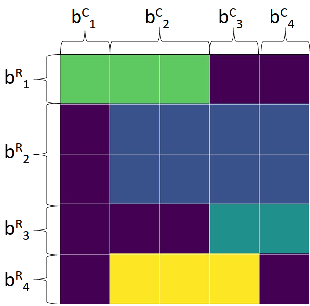
Finally, for our algorithms it will be convenient to operate on row and column blocks. For brevity, we only give the definition for row blocks. The row blocks partition the sets of rows, and they are defined such that each cluster can be expressed as the union of a set of blocks. More formally, for we let denote the set of indices of all row clusters that contain row . Now, the row block of is given by , i.e., it is the set of all rows that are contained in exactly the same row clusters as . Next, the set of row blocks is given by ; see Fig. 3 for an example. Given a row block it will be convenient for us to write to denote the row clusters in which is contained, i.e., for all . For column blocks, we define , and in the same way.
Visualizing weighted and directed graphs. The algorithm we propose in this paper is tailored to visualize unweighted bipartite graphs, through their Boolean biadjacency matrix . We note that since in general is asymmetric, our algorithms can also be used to visualize the adjacency matrix of directed graphs (note that in this case the set of row and column clusters will be the identical). It is also possible to use our algorithm to visualize weighted graphs; however, in this case one has to make adjustments to the coloring scheme to visualize the different weights (here, we focus on the Boolean case in which we never need more than six colors).
3 Visualization Objectives
In this section, we introduce our objective functions that measure different aspects of how well a biclustering is visualized.
Recall that biclusters represent pairs of elements that relate to each other. An ideal depiction of a single bicluster consists of a single large consecutive rectangle in the visualized matrix. More formally, we would like to have that and . However, when the row or column clusters of a biclustering overlap, obtaining a visualization which simultaneously presents all biclusters ideally is not possible (see, e.g., Fig. 2c). Thus, we have to define criteria that enable us to compare non-ideal depictions of biclusters.
Informally, the three criteria that we study are as follows:
- 1.
Proximity: All rows and columns of each bicluster should be close to each other, as shown in Fig. 2a.
- 2.
Size of the consecutive cluster areas: The rows and columns of each bicluster should form large consecutive areas, as shown in Fig. 2b.
- 3.
Size of uninterrupted areas: Areas that belong to (possibly different) biclusters should form large uninterrupted areas, as shown in Fig. 2c. Unlike the previous objectives, this objective is global, i.e., it is not limited to individual biclusters.


The formal definitions follow below. Note that even though the first and second criteria look similar at first, they are different: even when a bicluster is visualized with low proximity, it may still consist of several non-consecutive areas. Furthermore, the third criterion is particularly important when dealing with non-overlapping biclusterings; it will be useful, for instance, when visualizing biclusterings that have non-overlapping row clusters but overlapping column clusters, which is not captured by the previous two definitions. Previous work focused on proximity [13, 4] and also implicitly the consecutive area [4].
Next, we formally present three different objective functions, one for each criterion. Having different objective functions, instead of a single combined one, allows a more fine-grained evaluation of the visualizations.
Proximity. Our first objective function measures proximity. As stated above, our intuition is that for each bicluster, all of its rows and columns should be close to each other. To capture this intuition, we want to visualize the biclusters so that the convex hull of rows and columns that belong to the bicluster is small.
Consider permutations and and a bicluster . The size of the convex hull of in the biadjacency matrix is given by
| (1) |
Observe that for a single bicluster this quantity is minimized when it is visualized as a single consecutive rectangle, i.e., and . See also Fig. 3.
For all biclusters, our objective function for minimizing the proximity is
| (2) |
Size of the consecutive cluster areas. Next, we consider the aspect that the rows and columns of the same bicluster should form large consecutive areas.
First observe that when we visualize a bicluster under permutations and , then the consecutive areas are given by . For instance, if and , then the consecutive areas are .
Given this observation, we define the score for a single bicluster under the permutations and as follows:
| (3) |
In this score, we sum over the squared areas of the induced submatrices. Note that maximizing this score incentivizes layouts with larger consecutive areas. In particular, is maximized iff the bicluster is visualized as a single connected component, i.e., when the rows and columns in and are consecutive. Also observe that if in the score we summed over instead of , the sum would be independent of the permutations and always equal to ; this is why we sum over .
The corresponding global objective function is:
| (4) |
Size of uninterrupted areas. Lastly, we introduce an objective function which incentivizes that areas that belong to (possibly different) biclusters should form large uninterrupted areas. This is for useful for visualizing biclusters that are similar but non-overlapping, e.g., because they have disjoint row clusters but highly similar column clusters.
Recall that and are the row and column blocks, respectively. Since splitting up elements of blocks would only be detrimental to our visualizations, we henceforth assume that the elements from all row and column blocks are consecutive in our permutations, i.e., and for all and .
Now consider a row block and the submatrix which it induces. Observe that in this submatrix, column is contained in a bicluster if and , i.e., if is from a column block which co-occurs in a bicluster together with a row block . Similarly, if for with then column is not contained in a bicluster. Thus, the set of all columns in which are contained a bicluster after applying the permutation is . See Fig. 3 for an example. Thus, the size of the uninterrupted area of columns in biclusters in is given by
| (5) |
Notice the similarity of (5) and (3) above. The main difference is that in (3) we sum over the areas induced by the biclusters, whereas here we sum over the area induced by columns inside biclusters, regardless of bicluster membership. This is beneficial since when row block co-occurs with column block and with column block , then this definition incentivizes to place the column blocks and next to each other, even though they might not share a bicluster (i.e., even when ), which is not covered by (3).
Similar to above, we also want to measure the area of consecutive rows that appear in a bicluster in a submatrix that is induced by a fixed column cluster . We thus define and set .
Now our overall objective function becomes:
| (6) |
4 Algorithms
In this section, we describe our algorithms to obtain the permutations and that optimize our objective functions.
For better efficiency, we focus on finding permutations in which the rows of row blocks are always consecutive (and the same holds for the columns of column blocks). Observe that this assumption is without loss of generality, i.e., splitting the elements of a row or column block into multiple consecutive parts will never improve the objective functions we study.
Thus, suppose that we have row blocks . Then our new goal is to find a row block permutation that optimizes our objective functions.33 3 Note that we can turn the row block permutation into a row permutation as follows: For each , we fix an arbitrary order of the elements in . Now we create a list by iterating over and adding the elements in one after another to . If element is at the ’th position in , then we set . This will be more efficient since in practice . The same can be done for finding a column block permutation.
We present the pseudocode of our algorithms in Appendix A.
4.1 Greedy Algorithms
We start by considering a simple greedy algorithm for optimizing the three objective functions from Sect. 3. Our algorithm starts by sorting the row and column blocks based on their importance. Here, the importance score of a block is the sum of the area of the biclusters belongs to, i.e., . The idea is that blocks which are involved in large clusters are treated first and thus have priority when picking their position.
The greedy algorithm computes the row and column block permutations and simultaneously. Initially, they are set to the empty permutations and without any elements. Now the greedy algorithm proceeds in iterations until all row and column blocks have been assigned to the permutations. In iteration , we add the row (column) block with ’th highest importance to (). To pick the position of , we iterate over and consider the permutation with added in the ’th position. Then we insert in the position that achieved the best objective function value.
We note that while building the permutations above, they only map to the subset of the rows and columns that are contained in the row and column blocks that were assigned to the permutations. Therefore, to compute the objective function values, we only consider rows and columns that are contained in blocks that were already added to the permutations. Details and pseudocode are available in Appendix A.1.
4.2 Demerit-Based Algorithms
In practice, the greedy algorithm can be inefficient as it recomputes the objective functions several times during each iteration and each such recomputation requires a global pass over all clusters and blocks.
To remedy this problem, next we introduce the notion of demerit, which can be optimized locally and which acts as a penalty function for placing dissimilar blocks next to each other. Formally, the demerit for row block and column blocks and is given by:
where and . Observe that the demerit is a penalty term that measures the size of the row block and how dissimilar the blocks and are in terms of their cluster membership, i.e., it counts the number of clusters which contain row block but only exactly one of and .
To measure the demerit of the column block permutation , we set
where is the number of column blocks. This is the overall penalty incurred across all row blocks for column blocks that are placed next to each other. Optimizing this objective function should be somewhat simpler than the previous ones, because we only have to consider consecutive pairs of column blocks and , which can be checked locally. This is in contrast to our previous objective functions, which have to globally take into account all blocks that belong to a single bicluster (proximity and consecutive cluster area) or all blocks that appear consecutively (uninterrupted area).
Next, we introduce algorithms for minimizing the demerit, where we assume that we have a fixed row block permutation and we wish to compute an improved ordering of the column blocks . The same procedure can be used for fixed and for finding with small demerit. Details of both algorithms are available in Appendix A.2.
TSP heuristic. We first consider a TSP (traveling salesperson) heuristic to find a permutation that minimizes the demerit. First, we construct a complete graph containing all column blocks as nodes. For two column blocks and , we set the weight of the corresponding edge to which corresponds to the demerit of placing and next to each other. This is a complete graph, i.e., there are edges for all pairs of column blocks. Then we use a TSP solver to find a TSP tour in the corresponding graph, which is given by a cycle that visits every vertex exactly once. This corresponds to a column block permutation . Since the objective of TSP is to minimize the cost of the cycle, this corresponds to minimizing the demerit. Note that for defining , we can start with any of the blocks from the cycle, i.e., we can set for any and then proceed in the order of the cycle. To obtain the best results in practice, we pick the value which maximizes the cluster area (4).
Greedy demerit algorithm. We also consider a greedy algorithm which orders the blocks by their importance score and inserts them one by one. When inserting a block, it tries out all possible positions and picks the one which minimizes the total demerit.
4.3 Post-Processing: Suggesting Unclustered Rows and Columns
Finally, we present a post-processing scheme that finds unclustered rows and columns that have high similarity with existing biclusters. This will enable domain experts to easily identify structures which might have been missed by the biclustering algorithm. We describe our post-processing scheme for finding unclustered rows whose 1-entries have high similarity to existing column clusters; it can also be used for finding columns that are similar to existing row clusters.
We say that a row is unclustered if it is not contained in any row cluster, i.e., if , and we write to denote the set of unclustered rows. For , we write to denote the columns of all 1-entries in . Now the similarity of and a column cluster is given by , i.e., it measures the fraction of elements from that also appear in . Furthermore, the density of a bicluster is , i.e., it is the average number of non-zero entries in the submatrix induced by .
Now our idea is to create biclusters , which consist of unclustered rows and “original” column clusters . Here, we assign a row to if . This encodes the intuition that the rows in are allowed to be slightly sparser than those in the original bicluster ; for a domain expert it might be interesting to inspect them because the original biclustering algorithm might have “missed” them.
In the visualization, these new biclusters have a special place. The original biclusters are situated in the middle of the figure. Then, adjacent to that central part, the new biclusters and are added, and then the remaining unclustered rows and columns follow.
5 Experiments
We implemented our algorithms in Python and we practically evaluate them on real-world datasets. The source code1 and the plots2 of all biclusterings are available on GitHub. The experiments were performed on a 40-core Intel(R) Xeon(R) CPU E5-2630 v4 @ 2.20GHz.
The datasets we used are listed in Table 1, where we focussed on small- to medium-sized datasets since visualizing very large datasets requires other techniques [23]. We note that for 20news and movieLens we only considered the top- densest rows and columns to reduce the size of the datasets.
| dataset | rows | columns | density | ref. |
|---|---|---|---|---|
| 20news | [24] | |||
| americas_large | [19] | |||
| americas_small | [19] | |||
| apj | [19] | |||
| dialect | [6, 7] | |||
| domino | [19] | |||
| fire1 | [19] | |||
| fire2 | [19] | |||
| healthcare | [19] | |||
| movieLens | [21] | |||
| Mushroom (sample) | [13] | |||
| paleo | [8] |
To obtain our biclusterings, we used the PCV algorithm [20], which returns non-overlapping row clusters but overlapping column clusters, and the basso algorithm [16], which returns overlapping row and column clusters. Both algorithms have a parameter that determines the number of clusters and we report the choice of for each experiment.
In some of our visualizations, we use a 6-color system to convey more information (e.g., Fig. 1, 5a and 5c). Each of the colors is associated with a distinct category of data in the visualization: clustered elements appear in green, unclustered elements that were picked in our post-processing step (Sect. 4.3) are red, and all remaining unclustered elements are blue. The dark tones of each color correspond to -entries in the original matrix.44 4 We picked the colors using color brewer [3], so that the core set of colors (excluding the post-processing step) is colorblind safe and print friendly. As there is no 6-colors set that is colorblind safe, the final set of colors only retains the print friendly property. This allows us to assert whether or not an element belongs to the biclustering and/or to the original data, and it further allows to assess the density of the clustered (and non-clustered) areas.
In our experiments, we consider four greedy algorithms for optimizing the objective functions, denoting them greedyProximity, greedyConsecutiveClustersArea, greedyUninterruptedArea, greedyDemerit. Our TSP-based algorithm is denoted TSPheuristic and to solve TSP we use a solver from Google OR tools [22]. We compare them against the state-of-the-art method ADVISER [4]. Since there was no code available for ADVISER, we implemented our own version of it, available with our software.
Qualitative Evaluation.


We start with the qualitative evaluation of the algorithms. Our findings in this section are twofold: our TSPheuristic provides better visualizations than ADVISER [4] and our objective functions indeed measure the aspects of the visualizations which they are supposed to measure.
First, let us briefly argue about the merit of visualizing biclusterings. In Fig. 4a, we present visualizations of Fire1 without any ordering and the visualization created using TSPheuristic. The unordered dataset hints that some rows and columns seem related. After using basso for biclustering with and reordering the data with TSPheuristic, we can easily see the relation between rows and columns, as well as notice sparser areas inside the biclusters.
Next, we consider biclusterings obtained from PCV, which returns non-overlapping row clusters but overlapping column clusters. Fig.s 1a and 1b depict visualizations of dialect and paleo using ADVISER and TSPheuristic. Since ADVISER’s objective function does not take into account uninterrupted areas, its visualization is much less coherent than the one by TSPheuristic. The uninterrupted areas objective function captures this aspect well, where TSPheuristic obtains an higher score on dialect and a higher score on paleo.
Now we consider basso’s more complex biclusterings for 20news with , which contains overlapping row and column clusters. In this case, TSPheuristic is more resilient than ADVISER w.r.t. the proximity of the bicluster elements. In Fig.s 5a and 5c, we show the convex hulls of the same bicluster in red. One can see that the representation of the cluster is more compact in the visualization generated from TSPheuristic, compared to ADVISER. This also translates to the proximity objective function, where TSPheuristic achieves a proximity score that is lower than that of ADVISER (note that optimizing the proximity is a minimization problem).
Next, let us consider the uninterrupted areas that are generated by the algorithms. In Fig.s 5b and 5d, the respective biclusters have a similar proximity score ( and ), but the visualization proposed by greedyDemerit is nicer, as all the clusters are drawn as one consecutive block. This is also highlighted by the objective function value for uninterrupted bicluster area, which is higher for greedyDemerit.
Finally, we highlight the usefulness of our coloring scheme and our post-processing step from Sect. 4.3 in Fig. 4b. The coloring scheme highlights the very dense areas that basso selected as biclusters in green. Then our post-processing scheme clearly indicates that the remaining unclustered rows and columns contain areas similar to the original clusters, but of slightly lower density, which could be worth considering when manually inspecting the clusters. We note that the dense area in the bottom right of the plot is not marked in red, since the corresponding submatrix was not considered as part of the bicluster by basso; we decided not to consider such areas in our post-processing step.
Quantitative Evaluation.


For the quantitative validation, we run basso and PCV on all datasets from Table 1 with to obtain biclusterings. We run all visualization algorithms for each of these biclusterings and compute our objective function values from Sect.s 3 and 4.2. We also compute the objective function visualisationCost from ADVISER [4]. All plots are available online.2
To obtain comparability across different datasets and different biclusterings, we use normalization: For each dataset and a fixed biclustering, we report the ratio , where is the visualization algorithm we consider, is the objective function value obtained by and is the set of all visualization algorithms. We subtract the which denotes the average objective function of five random permutations; this is motivated by the fact that even the worst possible visualization will achieve non-negligible scores in our objective functions since typically their values are lower bounded by the squares of the block sizes. Note that if , achieved the best objective function value among all algorithms we compare.
We report our experimental results in Fig. 6, where Fig. 6a presents the results on biclusterings that were generated by PCV and Fig. 6b presents the results on biclusterings that were generated by basso. We observe that TSPheuristic performs well across all objective functions, even though on the consecutiveClusterArea it is slightly outperformed by ADVISER. Notably, TSPheuristic performs significantly better for the uninterrupted area score compared to ADVISER, especially for the biclusterings that were computed by PCV; this corroborates our findings from the qualitative evaluation. We note that among the greedy algorithms, greedyDemerit is the best, which further underscores that using demerit to guide visualizations is a good idea. Furthermore, on both sets of experiments, TSPheuristic outperforms ADVISER on the visualisationCost objective function which is being optimized by ADVISER. We conclude that TSPheuristic provides the best tradeoff across the different datasets and objective functions.
Running Time Analysis.
Finally, we compare the running times of the algorithm on our largest dataset americas_large and report the running times in Fig. 7. We observe that ADVISER is the fastest method overall and the greedy algorithms which optimize our objective functions from Sec. 3 are slow since computing the objective functions is rather slow. For TSPheuristic, we see an offset of 40 seconds which is the time we spend on running the TSP solver; overall, it scales better than our greedy baselines and typically finishes in at most 1 minute.
6 Conclusion
We studied the visualization of overlapping biclusterings and identified three different aspects that good visualizations should satisfy: proximity of cluster elements, large consecutive areas consisting of cluster elements, and large uninterrupted areas of clusters. We provided objective functions that capture these goals and showed experimentally that the best trade-off between these competing aspects is achieved by optimizing the demerit, which aims to place rows and columns with similar cluster membership next to each other.
Acknowledgements
This research is supported by the EC H2020 RIA project SoBigData++ (871042) and the Wallenberg AI, Autonomous Systems and Software Program (WASP) funded by the Knut and Alice Wallenberg Foundation. Some of the computations were enabled by the National Academic Infrastructure for Supercomputing in Sweden (NAISS) and Swedish National Infrastructure for Computing (SNIC) partially funded by the Swedish Research Council through grant agreements no. 2022-06725 and 2018-05973.
Ethical Statement
Boolean matrix factorization and similar pattern mining techniques can be used to identify tightly-knit communities (biclusters) from bipartite networks, which can help authorities to identify terrorist networks or dissidents from inter-communication networks. They can also be used to identify people’s political opinions (e.g., by studying their social network behavior). The visualization methods discussed in this paper cannot be used for these actions directly, as they require the underlying mining algorithm, but they do facilitate the use of the mining algorithms in benign as well as nefarious purposes. We do consider that the overall positive effects of these methods greatly outweigh the problems caused by the as-such unavoidable negative use cases.
References
- [1] Alistarh, D., Iglesias, J., Vojnovic, M.: Streaming min-max hypergraph partitioning. In: NeurIPS. pp. 1900–1908 (2015)
- [2] Behrisch, M., Bach, B., Henry Riche, N., Schreck, T., Fekete, J.D.: Matrix reordering methods for table and network visualization. In: Comput. Graph. Forum. vol. 35, pp. 693–716. Wiley Online Library (2016)
- [3] Brewer, C.A., Harrower, M., Sheesley, B., Woodruff, A., Heyman, D.: Colorbrewer 2.0: color advice for cartography. The Pennsylvania State University. http://colorbrewer2. org/. Accessed 6(02), 2010 (2009)
- [4] Colantonio, A., Di Pietro, R., Ocello, A., Verde, N.V.: Visual role mining: A picture is worth a thousand roles. IEEE Trans. Knowl. Data Eng. 24(6), 1120–1133 (2011)
- [5] Dhillon, I.S.: Co-clustering documents and words using bipartite spectral graph partitioning. In: Data Min. Knowl. Discov. pp. 269–274 (2001)
- [6] Embleton, S., Wheeler, E.S.: Finnish dialect atlas for quantitative studies. J. Quant. Linguist. 4(1-3), 99–102 (1997)
- [7] Embleton, S.M., Wheeler, E.S.: Computerized dialect atlas of finnish: Dealing with ambiguity. J. Quant. Linguist. 7(3), 227–231 (2000)
- [8] Fortelius (coordinator), M.: New and old worlds database of fossil mammals (NOW). Online. http://www.helsinki.fi/science/now/ (2003)
- [9] Grothaus, G.A., Mufti, A., Murali, T.: Automatic layout and visualization of biclusters. Algorithms Mol. Biol. 1(1), 1–11 (2006)
- [10] Hartigan, J.A.: Direct clustering of a data matrix. J. Am. Stat. Assoc. 67(337), 123–129 (1972)
- [11] Hess, S., Morik, K., Piatkowski, N.: The PRIMPING routine - tiling through proximal alternating linearized minimization. Data Min. Knowl. Discov. 31(4), 1090–1131 (2017)
- [12] Hess, S., Pio, G., Hochstenbach, M., Ceci, M.: Broccoli: overlapping and outlier-robust biclustering through proximal stochastic gradient descent. Data Min. Knowl. Discov. pp. 1–35 (2021)
- [13] Jin, R., Xiang, Y., Fuhry, D., Dragan, F.F.: Overlapping matrix pattern visualization: A hypergraph approach. In: IEEE Int. Conf. Data Min. pp. 313–322 (2008)
- [14] Lucchese, C., Orlando, S., Perego, R.: Mining top-k patterns from binary datasets in presence of noise. In: SIAM Int. Conf. Data Min. pp. 165–176 (2010)
- [15] Madeira, S., Oliveira, A.: Biclustering algorithms for biological data analysis: a survey. IEEE/ACM Trans. Comput. Biol. Bioinform. 1(1), 24–45 (2004)
- [16] Miettinen, P., Mielikäinen, T., Gionis, A., Das, G., Mannila, H.: The discrete basis problem. IEEE Trans. Knowl. Data Eng. 20(10), 1348–1362 (2008)
- [17] Miettinen, P., Neumann, S.: Recent Developments in Boolean Matrix Factorization. In: International Joint Conference on Artificial Intelligence (2020)
- [18] Misue, K.: Drawing bipartite graphs as anchored maps. In: IEEE Pac. Vis. CRPIT, vol. 60, pp. 169–177 (2006)
- [19] Molloy, I., Li, N., Li, T., Mao, Z., Wang, Q., Lobo, J.: Evaluating role mining algorithms. In: Proc. ACM Symp. Access Control Model. Technol. pp. 95–104 (2009)
- [20] Neumann, S.: Bipartite stochastic block models with tiny clusters. In: Neural Inf. Process. Syst. pp. 3871–3881 (2018)
- [21] Pedregosa, F., Varoquaux, G., Gramfort, A., Michel, V., Thirion, B., Grisel, O., Blondel, M., Prettenhofer, P., Weiss, R., Dubourg, V., Vanderplas, J., Passos, A., Cournapeau, D., Brucher, M., Perrot, M., Duchesnay, E.: Scikit-learn: Machine learning in Python. J. Mach. Learn. Res. 12, 2825–2830 (2011)
- [22] Perron, L., Furnon, V.: Or-tools, https://developers.google.com/optimization/
- [23] Pezzotti, N., Fekete, J., Höllt, T., Lelieveldt, B.P.F., Eisemann, E., Vilanova, A.: Multiscale visualization and exploration of large bipartite graphs. Comput. Graph. Forum 37(3), 549–560 (2018)
- [24] Rennie, J.: 20 newsgroups, http://qwone.com/˜jason/20Newsgroups/
- [25] Sakai, R., Winand, R., Verbeiren, T., Vande Moere, A., Aerts, J.: Dendsort: Modular leaf ordering methods for dendrogram representations in r. F1000Research 3, 177 (07 2014)
- [26] Sun, M., Zhao, J., Wu, H., Luther, K., North, C., Ramakrishnan, N.: The effect of edge bundling and seriation on sensemaking of biclusters in bipartite graphs. IEEE Trans. Vis. Comput. Graph. 25(10), 2983–2998 (2019)
- [27] Tatti, N., Miettinen, P.: Boolean matrix factorization meets consecutive ones property. In: SIAM Int. Conf. Data Min. pp. 729–737 (2019)
- [28] Vehlow, C., Beck, F., Weiskopf, D.: Visualizing group structures in graphs: A survey. Comput. Graph Forum 36 (2017)
- [29] Xu, P., Cao, N., Qu, H., Stasko, J.: Interactive visual co-cluster analysis of bipartite graphs. IEEE Pac. Vis. pp. 32–39 (2016)
- [30] Xu, P., Cao, N., Qu, H., Stasko, J.T.: Interactive visual co-cluster analysis of bipartite graphs. In: IEEE Pac. Vis. pp. 32–39 (2016)
- [31] Zha, H., He, X., Ding, C.H.Q., Gu, M., Simon, H.D.: Bipartite graph partitioning and data clustering. In: ACM Int. Conf. Inf. Knowl. Manag. pp. 25–32 (2001)
Appendix A Pseudocode
A.1 Pseudocode for the Greedy Algorithms
In the pseudocode, we write and to denote the number of elements which are currently contained in the permutation. When we add elements to the permutations, we write to denote the permutation with element added at the th position.
We use partialScore to denote the objective function values, but only defined on the elements which are contained in the (partial) permutations and , i.e., we ignore elements that have not yet been added to the permutations. For instance, for the greedy algorithm optimizing , will return the value of restricted to and .
We define greedyAddRow in Algorithm 2. greedyAddColumn is defined in a similar manner, by adding the element in the column permutation instead of in the row permutation .
A.2 Pseudocode for Demerit-Based Algorithms
Algorithm 3 presents the details of our TSP heuristic for minimizing the demerit. Algorithm 4 presents the details of our greedy algorithm for minimizing the demerit, which is inspired by the algorithm of [4]. We define based on the definition of in Section 4.2: