Unsourced Random Access Using Multiple Stages of Orthogonal Pilots: MIMO and Single-Antenna Structures
Abstract
We study the problem of unsourced random access (URA) over Rayleigh block-fading channels with a receiver equipped with multiple antennas. We propose a slotted structure with multiple stages of orthogonal pilots, each of which is randomly picked from a codebook. In the proposed signaling structure, each user encodes its message using a polar code and appends it to the selected pilot sequences to construct its transmitted signal. Accordingly, the transmitted signal is composed of multiple orthogonal pilot parts and a polar-coded part, which is sent through a randomly selected slot. The performance of the proposed scheme is further improved by randomly dividing users into different groups each having a unique interleaver-power pair. We also apply the idea of multiple stages of orthogonal pilots to the case of a single receive antenna. In all the set-ups, we use an iterative approach for decoding the transmitted messages along with a suitable successive interference cancellation technique. The use of orthogonal pilots and the slotted structure lead to improved accuracy and reduced computational complexity in the proposed set-ups, and make the implementation with short blocklengths more viable. Performance of the proposed set-ups is illustrated via extensive simulation results which show that the proposed set-ups with multiple antennas perform better than the existing MIMO URA solutions for both short and large blocklengths, and that the proposed single-antenna set-ups are superior to the existing single-antenna URA schemes.
Index Terms:
Unsourced random access (URA), internet of things (IoT), orthogonal pilots, massive MIMO, pilot detection, power diversity, CRC check, performance analysis, fading channel.I Introduction
In contrast to the conventional grant-based multiple access, where the base station (BS) waits for the preamble from devices to allocate resources to them, in grant-free random access, users transmit their data without any coordination. Removing the need for scheduling results in some benefits, such as reducing the latency and signaling overhead, which makes the grant-free set-up interesting for serving many users. Sourced and unsourced random access schemes are the main categories of grant-free random access. In the former, both the messages and identities of the users are important to the BS, so each user is assigned a unique pilot. However, this is inefficient, especially considering the next-generation wireless networks with a massive number of connected devices [1, 2]. In the so-called unsourced random access (URA), which was introduced by Polyanskiy in [3], the BS cares only about the transmitted messages, i.e., the identity of the users is not a concern. The BS is connected to millions of cheap devices, a small fraction of which are active at a given time. In this set-up, the users employ a common codebook, and they share a short frame for transmitting their messages. In URA, the per-user probability of error (PUPE) is adopted as the performance criterion.
Many low-complexity coding schemes are devised for URA over a Gaussian multiple-access channel (GMAC) including T-fold slotted ALOHA (SA) [4, 5, 6, 7], sparse codes [8, 9, 10, 11], and random spreading [12, 13, 14]. However, GMAC is not a fully realistic channel model for wireless communications. Therefore, in [15, 16, 17, 18, 19], the synchronous Rayleigh quasi-static fading MAC is investigated, and the asynchronous set-up is considered in [20, 21]. Recently, several studies have investigated Rayleigh block-fading channels in a massive MIMO setting [22, 23, 24, 25]. In [22], a covariance-based activity detection (AD) algorithm is used to detect the active messages. A pilot-based scheme is introduced in [23] where non-orthogonal pilots are employed for detection and channel estimation, and a polar list decoder is used for decoding messages. Furthermore, in a scheme called FASURA [24], each user transmits a signal containing a non-orthogonal pilot and a randomly spread polar code.
The coherence blocklength is defined as the period over which the channel coefficients stay constant. As discussed in [23], the coherence time can be approximated as , where is the maximal Doppler spread. For a typical carrier frequency of GHz, the coherence time may vary in the range of ms– ms (corresponding to the transmitter speeds between km/h– km/h). Moreover, the sampling frequency should be chosen in the order of coherence bandwidth, whose typical value is between kHz– kHz in outdoor environments. Consequently, the coherence blocklength can range from to samples. Although the AD algorithm in [22] performs well in the fast fading scenario (e.g., when ), it is not implementable with larger blocklengths due to run-time complexity scaling with . In contrast, the schemes in [23, 24] work well in the large-blocklength regimes (e.g., for ); that is, in a slow fading environment where large blocklengths can be employed, their decoding performance is better than that of [22].
Most coding schemes in URA employ non-orthogonal pilots/sequences for identification and estimation purposes [22, 13, 14, 23, 12, 24]. Performance of detectors and channel estimators may be improved in terms of accuracy and computational complexity by employing a codebook of orthogonal pilots; however, this significantly increases the amount of collisions due to the limited number of available orthogonal pilot sequences. To address this problem, the proposed schemes in this paper employ multiple stages of orthogonal pilots combined with an iterative detector.
In the proposed scheme, the transmitted signal of each user is composed of stages: a polar codeword appended to independently generated orthogonal pilots. Thus, the scheme is called multi-stage set-up with multiple receive antennas (MS-MRA). At each iteration of MS-MRA at the receiver side, only one of the pilot parts is employed for pilot detection and channel estimation, and the polar codeword is decoded using a polar list decoder. Therefore, the transmitted pilots in the remaining pilot parts are still unknown. To determine the active pilots in these, we adopt two approaches. In the first one, all the pilot bits are coded jointly with the data bits and cyclic redundancy check (CRC) bits (therefore, the transmitted bits of all the pilot parts are detected after successful polar decoding). As a second approach, to avoid waste of resources, we propose an enhanced version of the MS-MRA, where only data and CRC bits are fed to the polar encoder. At the receiver side, the decoder iteratively moves through different parts of the signal to detect all the parts of an active user’s message. Since it does not encode the pilot bits, this is called MS-MRA without pilot bits encoding (MS-MRA-WOPBE). We further improve the performance of the MS-MRA by randomly dividing users into different groups. In this scheme (called multi-stage set-up with user grouping for multiple receive antennas (MSUG-MRA)), each group is assigned a unique interleaver-power pair. Transmission with different power levels increases the decoding probability of the users with the highest power (because they are perturbed by interfering users with low power levels). Since successfully decoded signals are removed using successive interference cancellation (SIC), users with lower power levels have increased chance of being decoded in the subsequent steps. By repeating each user’s signal multiple times, we further extend the idea in MS-MRA and MSUG-MRA to the case of a single receive antenna. These extensions are called multi-stage set-up with a single receive antenna (MS-SRA) and multi-stage set-up with user grouping for a single receive antenna (MSUG-SRA).
We demonstrate that, while the covariance-based AD algorithm in [22] suffers from performance degradation with large blocklengths, and the algorithms in [23, 24] do not work well in the short blocklength regime (hence not suitable for fast fading scenarios), the MS-MRA and MSUG-MRA have a superior performance in both regimes. Furthermore, the MS-SRA and MSUG-SRA show better performance compared to similar solutions with a single receive antenna over fading channels [17, 20, 19].
Our contributions are as follows:
- •
We propose a URA set-up with multiple receive antennas, namely MS-MRA. The proposed set-up offers comparable performance with the existing schemes with large blocklengths, while having lower computational complexity. Moreover, for the short-blocklength scenario, it significantly improves the state-of-the-art.
- •
We provide a theoretical analysis to predict the error probability of the MS-MRA, taking into account all the sources of error, namely, errors resulting from pilot detection, channel estimation, channel decoding, SIC, and collisions.
- •
We extend the MS-MRA set-up by randomly dividing the users into groups, i.e., MSUG-MRA, which is more energy-efficient than MS-MRA and other MIMO URA schemes.
- •
Two URA set-ups with a single receive antenna, called MS-SRA and MSUG-SRA, are provided by adopting the ideas of the MS-MRA and MSUG-MRA to the case of a single receive antenna. They perform better than the alternative solutions over fading channels.
The rest of the paper is organized as follows. Section II presents the system model for the proposed framework. The encoding and decoding procedures of the proposed schemes are introduced in Section III. In Section IV, extensive numerical results and examples are provided. Finally, Section V provides our conclusions.
The following notation is adopted throughout the paper. We denote the sets of real and imaginary numbers by and , respectively. and represent the th row and the th column of , respectively; the and give the real and imaginary parts of , respectively; the transpose and Hermitian of matrix are denoted by and , respectively; denotes the cardinality of a set, and denote the identity matrix and all-ones vector, respectively; we use to denote , and is the Kronecker delta.
II System Model
We consider an unsourced random access model over a block-fading wireless channel. The BS is equipped with receive antennas connected to potential users, for which of them are active in a given frame. Assuming that the channel coherence time is larger than , we divide the length- time-frame into slots of length each (). Each active user randomly selects a single slot to transmit bits of information. In the absence of synchronization errors, the received signal vector corresponding to the th slot at the th antenna is written as
| (1) |
where , denotes the set of active user indices available in the th slot, , is the encoded and modulated signal corresponding to the message bit sequence of the th user, is the channel coefficient between the th user and the th receive antenna, and is the circularly symmetric complex white Gaussian noise vector. Letting and be the set of active user indices and the list of decoded messages, respectively, the PUPE of the system is defined in terms of the probability of false-alarm, , and the probability of missed-detection, , as
| (2) |
where and , with being the number of decoded messages that were indeed not sent. The energy-per-bit of the set-up can be written as , where denotes the average power of each user per channel use. The objective is to minimize the required energy-per-bit for a target PUPE.
III URA with Multiple Stages of Orthogonal Pilots
III-A MS-MRA Encoder
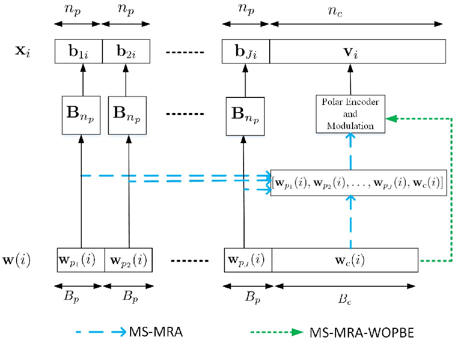
In this part, we introduce a multi-stage signal structure which is used in both of the proposed URA set-ups. As shown in Fig. 1, we divide the message of the th user into parts (one coded part and pilot parts) denoted by and with lengths and , respectively, where . The th user obtains its th pilot sequence, , with length by mapping to the orthogonal rows of an Hadamard matrix , which is generated as
where represents the Kronecker product. Since the number of possible pilots in the orthogonal Hadamard codebook is limited, it is likely that the users will be in collision in certain pilot segments, that is, they share the same pilots with the other users. However, the parameters are chosen such that two different users are in a complete collision in all the pilot parts with a very low probability. To construct the coded sequence of the th user, we accumulate all the message bits in a row vector as
| (3) |
and pass it to an polar code, where is the number of CRC bits. Note that contrary to the existing schemes in URA, we feed not only data bits but the pilot bit sequences to the encoder. Hence, in the case of successful decoding, all the pilot sequences for the user can be retrieved. The polar codeword is then modulated using quadrature phase shift keying (QPSK), resulting in , where is the average power of the polar coded part, and Gray mapping is used. The overall transmitted signal for the th user consists of pilot parts and one coded part, i.e.,
| (4) |
where and denotes the average power of the pilot sequence. Accordingly, the received signal in a slot is composed of parts, for which, at each iteration, the decoding is done by employing one of the pilot parts (sequentially) and the coded part of the received signal. Generally, only the non-colliding users can be decoded. Some non-colliding users in the current pilot stage may experience collisions in the other pilot parts. Therefore, by successfully decoding and removing them using SIC, the collision density is reduced, and with further decoding iterations, the effects of such collisions are ameliorated.
III-B MS-MRA Decoder
We now introduce the decoding steps of MS-MRA where the transmitted signal in (4) is received by antennas through a fading channel. The th pilot part and the polar coded part of the received signal in the th slot of the MS-MRA can be modeled using (1) as
| (5) | ||||
| (6) |
where is the channel coefficient matrix with in its th row and th column, and consist of independent and identically distributed (i.i.d.) noise samples drawn from (i.e., a circularly symmetric complex Gaussian distribution), and and determine the rows of and , respectively, with . Note that we have removed the slot indices from the above matrices to simplify the notation.
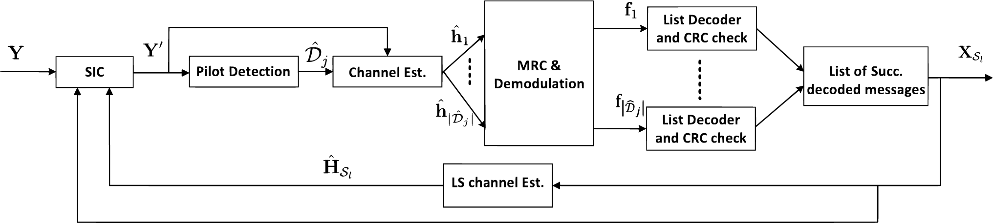
The decoding process is comprised of five different steps that work in tandem. A pilot detector based on a Neyman-Pearson (NP) test identifies the active pilots in the current pilot part; channel coefficients corresponding to the detected pilots are estimated using a channel estimator; maximum-ratio combining (MRC) is used to produce a soft estimate of the modulated signal; after demodulation, the signal is passed to a polar list decoder; and, the successfully decoded codewords are added to the list of successfully decoded signals before being subtracted from the received signal via SIC. The process is repeated until there are no successfully decoded users in consecutive SIC iterations. In the following, and denote the received signals in (5) and (6) after removing the list of messages successfully decoded in the current slot up to the current iteration.
III-B1 Pilot Detection Based on NP Hypothesis Testing
At the th pilot part, we can write the following binary hypothesis testing problem:
| (7) |
where , , with , and are alternative and null hypotheses that show the existence and absence of the pilot at the th pilot part, respectively, and is the number of users that pick the pilot as their th pilots.
Lemma 1.
([25, Appendix A]): Let be the estimate of the set of active rows of in the th pilot part. Using a level Neyman-Pearson hypothesis testing (where is the bound on the false-alarm probability), can be obtained as
| (8) |
where , denotes the cumulative distribution function of the chi-squared distribution with degrees of freedom , and is its inverse.
The detection probability of a non-colliding user () is then obtained as
| (9) |
where in (a), we use the fact that . Note that a higher probability of detection is obtained in the general case of . It is clear that the probability of detection is increased by increasing the parameters , , , and .
III-B2 Channel Estimation
Let be a sub-matrix of consisting of the detected pilots in (8), and suppose that is the corresponding pilot of the th user. Since the rows of the codebook are orthogonal to each other, the channel coefficient vector of the th user can be estimated as
| (10) |
If the th user is in a collision ( ), (10) gives an unreliable estimate of the channel coefficient vector. However, this is not important since a CRC check is employed after decoding and such errors do not propagate.
III-B3 MRC, Demodulation, and Channel Decoding
Let be the channel coefficient vector of the th user, where with denoting the set of remaining users in the th slot. Using in (10), the modulated signal of the th user can be estimated employing the MRC technique as
| (11) |
Plugging (6) into (11), is written as
| (12) |
where . The first and second terms on the right-hand side of (12) are the signal and interference-plus-noise terms, respectively. We can approximate to be Gaussian distributed, i.e., , where , which is obtained by treating the coded data sequences of different users to be uncorrelated. The demodulated signal can be obtained as
| (13) |
where . From (12) and (13), and using , each sample of can be approximated as , where . The following log-likelihood ratio (LLR) is obtained as the input to the polar list decoder
| (14) |
where is an approximation of which is obtained by replacing ’s by their estimates. At the th pilot part, the th user is declared as successfully decoded if 1) its decoder output satisfies the CRC check, and 2) by mapping the th pilot part of its decoded message to the Hadamard codebook, is obtained. Then, all the successfully decoded messages (in the current and previous iterations) are accumulated in the set , where .
III-B4 SIC
we can see in (3) that the successfully decoded messages contain bit sequences of pilot parts and the coded part ( and ). Having the bit sequences of successfully decoded messages, we can construct the corresponding transmitted signals using (4). The received signal matrix can be written as
| (15) |
where is obtained by merging received signal matrices of different parts, i.e.,
with and including the signals in the sets and , and and comprising the channel coefficients corresponding to the users in the sets and , respectively. Employing the least squares (LS) technique, is estimated as
| (16) |
Note that consists of all the successfully decoded signals in the th slot so far, and is the initially received signal matrix (not the output of the latest SIC iteration). The SIC procedure is performed as follows
| (17) |
Finally, is fed back to the pilot detection algorithm for the next iteration, where the next pilot part is employed. We note that if no user is successfully decoded in consecutive iterations (corresponding to different pilot parts), the algorithm is stopped. The details of the decoding stages of MS-MRA are shown in Fig. 2 and Algorithm 1. Note that we will discuss MS-MRA-WOPBE, which deviates from the above model, in Section III-D.
Theorem 1.
The signal-to-interference-plus-noise ratio (SINR) at the output of MRC for a non-colliding user in the th slot can be approximated as
| (18) |
where if the transmitted signals are randomly interleaved, and , , otherwise, with .
Proof.
See Appendix A. ∎
We employ the above approximate SINR expression 1) to estimate the error probability of MS-MRA analytically, and 2) to determine the optimal power allocation for each group in MSUG-MRA. We further note that using this SINR approximation, the performance of the MS-MRA is well predicted in the low and medium regimes (see Fig. 6). The reason why the SINR approximation does not work well in the high regime is the employed approximations in Lemma 4 (see the Appendix A for details).
.
( denotes the iteration index).
while do
Ch. estimation: estimate channel coefficient using (10).
if MS-MRA then
Demodulation: obtain using (13).
Decoding: pass in (14) to list decoder.
end for
.
LS-based ch. estimation: estimate using (16).
SIC: update and using (17). end for
III-C Analysis of MS-MRA
In this part, the PUPE of the MS-MRA is analytically calculated, where errors resulting from the collision, pilot detection, and polar decoder are considered. For our analyses, we assume that after successfully decoding and removing a user using a pilot part, the decoder moves to the next pilot part. Hence, in the th iteration of the th slot, we have
| (19a) | ||||
| (19b) | ||||
Lemma 2.
Let be the event that out of users remain in the th slot, and define , where . Assuming that the strongest users with highest values are decoded first, we have
| (20) |
where , with denoting the PDF of the chi-squared distribution with degrees of freedom and .
Proof.
In the first iteration of the th slot for which no user is decoded yet (all the active users are available), since , we have . We assume that the users with higher values of are decoded first. Hence, if in an iteration, out of users remain in the slot, the distribution of is obtained by where removes portion of the samples with higher values from the distribution and normalizes the distribution of the remaining samples, i.e.,
where is obtained by solving the following equation , which results in . Therefore, we obtain
| (21) |
∎
We can see from (13) and (14) that the input of the polar decoder is a real codeword. Thus, the average decoding error probability of a non-colliding user in the th iteration of a slot with users can be approximated as (see [27])
| (22) |
where denotes the standard -function, and is the SINR of a non-colliding user in the th iteration of a slot with users, which is calculated using Theorem 1, Lemma 2, and (19) as
| (23) |
where and . Note that since the powers of signal and interference-plus-noise terms of are equal in their real and imaginary parts, the SINRs of in (14) and are the same. Therefore, in (22), we employ the SINR calculated in Theorem 1 for the input of the polar list decoder.
Since decoding in the initial iterations well represents the overall decoding performance of the MS-MRA, we approximate the SINR of the first iteration by setting in (23) as
| (24) |
Concentrating on (22), we notice that is a decreasing function of and . Besides, (24) shows that increases by decreasing and (considering ), and increasing , , and , however, it is not a strictly monotonic function of . Since our goal is to achieve the lowest by spending the minimum , we can optimize the parameters , , , and .
Theorem 2.
In the th iteration of the th slot, the probability of collision for a remaining user can be approximated as
| (25) |
where denotes the average number of pilots that are in -collision (selected by different users) in the th iteration, which is calculated as
| (26) |
where , and with denoting the probability mass function (PMF) of the Poisson distribution with the parameter .
Proof.
See Appendix B. ∎
Note that to extend the result in Theorem 2 to an SIC-based system with only one pilot sequence (orthogonal or non-orthogonal), we only need to set in the above expressions. From (25), the collision probability in the first iteration can be calculated as , which is a decreasing function of . Since the overall decoding performance of the system depends dramatically on the collision probability in the first iteration, we can increase , however, this results in additional overhead.
Corollary 1.
Note that the result in Corollary 1 can also be used in any other slotted system with SIC by replacing appropriate .
III-D MS-MRA-WOPBE
As discussed in Section III-A, in the MS-MRA scheme, the pilot bits are fed to the polar encoder along with the data and CRC bits. To improve the performance by decreasing the coding rate, the MS-MRA-WOPBE scheme passes only the data and CRC bits to the encoder. To detect the bit sequences of different parts of the message, it employs an extra iterative decoding block called iterative inter-symbol decoder (IISD) (described in Section III-D2). At each step of IISD, it detects one part of a user’s signal (polar or pilot part), appends the detected part to the current pilot (which was used for channel estimation in the previous step) to have an extended pilot, and re-estimates the channel coefficients accordingly. The encoding and decoding procedures of MS-MRA-WOPBE are described below.
III-D1 Encoder
The th user encodes its bits using the following steps (the general construction is shown in Fig. 1). Similar to the MS-MRA encoder in Section III-A, information bits are divided into parts as in (3), and the transmitted signal is generated as in (4). The only difference is in the construction of the QPSK signal. The encoder in MS-MRA-WOPBE defines two CRC bit sequences as and , where and are generator matrices known by the BS and users. Then, it passes to an polar encoder, and modulates the output by QPSK to obtain .
III-D2 Decoder
As shown in Algorithm 1, MS-MRA-WOPBE exploits the same decoding steps as the MS-MRA scheme, except for the IISD step. We can see in Algorithm 1 that the th pilot of the th user is detected before employing the IISD. Then, IISD must detect the data (polar) sequence and the th pilot of the th user, where . In the following, IISD is described in detail.
Step 1 [Detecting ]: We first obtain using (13), where , and . Then, we pass to the list decoder. A CRC check and an estimate of 11
1
In the output of the polar list decoder, there is a list of possible messages. If more than one messages satisfy the CRC check (), the most likely of them is returned as the detected message and the CRC flag is set to one. Otherwise, the most likely message is returned as the detected message and the CRC flag is set to zero. are obtained by the polar list decoder.
Step 2 [Updating ]: Since the th pilot and polar codeword of the th user are detected so far, we append them to construct a longer signal as . Then, we update by MMSE estimation as , where , and .
Step 3 [Detecting ]: Assuming that the th row of the Hadamard matrix is active in the th pilot part (), we estimate the corresponding channel coefficient as (see (10)). To find the th pilot sequence of the th user, we find the pilot whose corresponding channel coefficient vector is most similar to , i.e., we maximize the correlation between and as
| (30) |
Step4 [Updating ]: Since the bit sequences of all parts are detected, we can construct using (4). The channel coefficient vector can be updated by MMSE as , where . If the number of users that satisfy is not changed in an iteration, the iteration is stopped, otherwise, the algorithm goes to Step 1 for another iteration with updated . Users whose bit sequences satisfy and are added to the set as successfully decoded users of the current iteration.
III-E MSUG-MRA
Different from MS-MRA where the power of every user is the same and signals are not interleaved, MSUG-MRA defines groups, each being assigned unique interleaver and power pair (), . We assume that is constant in all groups, hence each group can be identified with a unique interleaver-power pair , which is known at both transmitter and receiver sides. The details of encoding and decoding procedures as well as the power selection strategy are explained below. Note that we assume without loss of generality that .
III-E1 Encoder
The encoding is adopted as follows:
- •
Every user randomly selects a group, e.g., with index .
- •
Each user employs and as the powers of the coded and pilot parts, with which it generates its multi-stage signal similar to MS-MRA (according to (4)).
- •
The transmitted signal is created as .
III-E2 Decoder
In each iteration, the decoder tends to decode the messages belonging to the users of the dominant group (the th group with the highest power level). After decoding and removing users in the th group, users in the st group become the dominant ones. Using the same trend, all the groups have the chance to be the dominant group at some point. Since users in different groups are interleaved differently, signals of users in other groups are uncorrelated from the signals in the dominant group. Thus, letting the th group to be dominant, we approximately model the th signal in the the th group () as
| (31) |
where . Therefore, when the th group is dominant (the users in the groups with indices greater than are already removed using SIC), users in the th group are perturbed by i.i.d. noise samples drawn from , with , where is the average number of users in each group of the current slot. Consequently, by replacing , , and with , , and in the decoding steps of MS-MRA (in Section III-B), the decoding procedure of MSUG-MRA is obtained as:
- •
Deinterleave the rows of the received signals: and .
- •
Find active pilots as
where .
- •
Channel estimation and MRC: , where , and is one of the detected pilots.
- •
Pass to the polar decoder, where , and is defined in (13).
- •
Regenerate signals of successfully decoded users according to Section III-E1 (using (,) pair), and collect them in the rows of .
- •
Apply LS-based SIC similar to (17), i.e., .
Note that this loop is repeated for different group indices and different pilot parts, and the iteration is stopped if there is no successfully decoded users in consecutive iterations.
III-E3 Power Calculation
When MSUG-MRA starts the decoding in the th group, there are successfully decoded users from previous groups (with higher power levels), users remain in the th group, and users in the current group are perturbed with a complex Gaussian noise with covariance matrix . Therefore, the SINR of a non-colliding user in the current group can be calculated by replacing , , , , , , , and in (18) as
| (32) |
where . To impose similar performance on different groups, we set . Solving this equation, the power of the th group satisfies , where , , . Solving this equation, we have
| (33) | ||||
Note that the MS-MRA scheme is a special case of the MSUG-MRA with .
III-F MS-SRA and MSUG-SRA
In this part, we apply the proposed MIMO coding schemes to the case of a single receive antenna. To accomplish this, we repeat each user’s length- signal multiple times to create temporal diversity in MS-SRA and MSUG-SRA. Accordingly, we divide the whole frame into sub-frames of length , then divide each sub-frame into slots of length . Each user randomly selects a slot index, namely , and transmits its signal, through the th slot of each sub-frame. Assuming the coherence time to be , each sub-frame is analogous to a receive antenna. Therefore, the transmitted messages in MS-SRA and MSUG-SRA can be decoded using MS-MRA and MSUG-MRA decoders in Sections III-B and III-E2, respectively, considering receive antennas. Since each user repeats its signal times, for this case, we have .
III-G Computational Complexity
We focus on the number of multiplications as a measure of the computational complexity, and make a complexity comparison among the proposed and existing URA solutions. The per-iteration computational complexity of the MS-MRA in a slot is calculated as follows: The pilot detection in (8) has a complexity of corresponding to different pilot parts and different slots, where is the standard big-O notation, denoting the order of complexity. The channel estimator in (10) does not require any extra computation, because corresponds to which is calculated before for pilot detection; the MRC in (11) has a complexity of ; to compute the LLR in (14), the required computational complexity is ; the computational complexity of the polar list decoder is [26] ; and, the SIC has a complexity of . We know from (44) that in the first iteration, we have , and ; in the last iterations, we have and . Hence, considering and , we can compute the computational complexity of the MS-MRA in the first and last iterations as and , respectively. Considering the computational complexity in the intermediate iterations to be in the same order, the per-iteration computational complexity of the MS-MRA can be bounded by . Note that the computational complexity of MSUG-MRA is in the same order as MS-MRA, and for MS-SRA and MSUG-SRA schemes, the computational complexity is obtained by replacing by in the above figures. Note that by employing a low-complexity adaptive filter [28, 29, 30], we can considerably reduce the computational complexity of the LS-based channel estimator in (16) (hence the total computational complexity of the proposed schemes).
Looking at Algorithm 1, we can infer that MS-MRA-WOPBE is obtained by employing the same pilot detector (with complexity ), channel estimator (does not incur any extra computational complexity), and SIC (with complexity ) as in the MS-MRA case, except for employing the IISD block. In Step 1 of IISD, the complexity for computing and implementing polar decoder are and , respectively, where denotes the number of iterations of IISD. In the Step 2 of IISD, computing and has the complexity of and , respectively. The computational complexity of obtaining in Step 3 of IISD is . Then, replacing and with their approximate values (discussed in the previous paragraph), the overall computational complexity of the MS-MRA-WOPBE is bounded by .
For comparison purposes, the dominant per-iteration computational complexity of the FASURA in [24] (which is due to energy detector and SIC operation) can also be computed as , where denotes the number of pilot bits, is the frame length, and is the length of the spreading sequence.
IV Numerical Results
We provide a set of numerical results to assess the performance of the proposed URA set-ups. In all the results, we set , the number of CRC bits , the Neyman-Pearson threshold , and the list size of the decoder to . For MS-MRA and MSUG-MRA, we set the frame length , and . The corresponding values for the MS-SRA and MSUG-SRA are , and .
In Fig. 3, the performance of the proposed MS-MRA and MSUG-MRA is compared with the short blocklength scheme of [22] with the number of antennas and slot length . (In this scenario, we consider a fast-fading environment, where the coherence blocklength is considered as ). To facilitate a fair comparison, we consider () and ( for MSUG-MRA) for all the proposed schemes. For MSUG-MRA, the value of is set as for , for , for , for , and for . The superiority of the proposed schemes over the one in [22] is mostly due to the more powerful performance of the polar code compared to the simple coding scheme adopted in [22] and the use of the SIC block, which significantly diminishes the effect of interference. We also observe that MS-MRA-WOPBE outperforms MS-MRA, which is due to 1) employing IISD, which iteratively improves the accuracy of the channel estimation, and 2) lower coding rate by not encoding the pilot bits. Besides, the range of the number of active users that are detected by the MSUG-MRA is higher than those of MS-MRA and MS-MRA-WOPBE schemes. This improvement results from randomly dividing users into different groups, which provides each group with a lower number of active users (hence a lower effective interference level).

In Fig. 4, we compare the proposed MS-MRA and MSUG-MRA with the ones in [23, 24], considering the slow-fading channel with coherence blocklength . We set , , for MS-MRA. We choose for , for , and for with . Thanks to employing the slotted structure, SIC, and orthogonal pilots, all the proposed schemes have superior performance compared to [23]. Due to employing random spreading and an efficient block called NOPICE, FASURA in [24] performs better than the proposed MS-MRA and MSUG-MRA in the low regimes; however, its performance is worse than the MSUG-MRA in higher values of (thanks to the random user grouping employed in MSUG-MRA). The proposed MS-MRA-WOPBE also shows a similar performance as FASURA. To achieve the result in Fig. 4, FASURA sets , , , , , and . The order of computational complexity for these schemes is given in the performance-complexity plot in Fig. 5. It can be interpreted from this figure that the proposed MS-MRA-WOPBE has comparable accuracy to FASURA while offering a lower computational complexity. Note also that despite the higher required compared to FASURA, MS-MRA offers very large savings in terms of computational complexity, which is attributed to employing orthogonal pilots, slotted structure, and simpler decoding blocks.


As a further note, FASURA considers possible spreading sequences of length for each symbol of the polar codeword; hence every transceiver should store vectors of length , as well as a pilot codebook of size . For typical values reported in [24], the BS and every user must store vectors of length and a matrix of size . For the proposed schemes in this paper, every transceiver must store only an orthogonal codebook of size , where . Thus, FASURA requires about 3000 times larger memory than our proposed schemes, which may be restrictive for some target URA applications such as sensor networks, where a massive number of cheap sensors are deployed. Moreover, unlike FASURA, the proposed solutions are implementable with short blocklengths (see Fig. 3), which makes them appropriate for fast fading scenarios as well.
In Fig. 6, we compare the theoretical PUPE in (27) with the simulation results of the MS-MRA for three different scenarios () with and . It is shown that the approximate theoretical analysis well predicts the performance of the MS-MRA for , however, the results are not consistent for higher values of . The reason for the mismatch for the regime is the approximations employed while analyzing SIC in Lemma 4 (e.g., , , uncorrelated QPSK codewords of two different users, and uncorrelated samples of ).

Fig. 7 compares the MS-SRA and MSUG-SRA with the existing single-antenna solutions [17, 20, 19]. For both set-ups, we set , ( for MSUG-SRA), for , and for . For MSUG-SRA, we also choose for , for , and for . It is observed that the proposed MS-SRA has a superior performance compared to the existing URA approaches for the low number of active users, However, it performs worse than the scheme in [19] for higher values of . Furthermore, the proposed MSUG-SRA outperforms existing solutions, and its effective range of is up to users.
V Conclusions
We propose a family of unsourced random access solutions for MIMO Rayleigh block fading channels. The proposed approaches employ a slotted structure with multiple stages of orthogonal pilots. The use of a slotted structure along with the orthogonal pilots leads to the lower computational complexity at the receiver, and also makes the proposed designs implementable for fast fading scenarios. We further improve the performance of the proposed solutions when the number of active users is very large by randomly dividing the users into different interleaver-power groups. The results show that the proposed MIMO URA designs are superior for both short and large blocklengths, while offering a lower computational complexity.
Appendix A Proof of Theorem 1
Lemma 3.
Assuming that the transmitted data part contains uncorrelated and equally likely QPSK symbols, for and , the transmitted signals satisfy
| (34) |
where .
Proof.
Let and be the th pilots of the th and th users, and and be the corresponding polar-coded and QPSK-modulated signals. Since and are randomly chosen rows of the Hadamard matrix, with probability , and it is zero with probability . Besides, for , and are zero-mean and uncorrelated, where . Therefore,
Note that, strictly speaking, the uncorrelated QPSK symbol assumption is not accurate for coded systems. Nevertheless, it is useful to obtain a good approximation of SINR, as we will show later. ∎

Lemma 4.
By applying LS-based SIC, the residual received signal matrices of pilot and coded parts can be written based on the signal and interference-plus-noise terms as
| (35) |
| (36) |
where is the channel coefficient vector of the th user, , , and the elements of and are drawn from and , respectively, with and are as defined in the statement of the Theorem 1.
Proof.
Plugging (15) and (16) into (17), we obtain
| (37) |
where , and . Since and , we have
| (38) |
Since the values of and are large, and using (34), we have , where . In other words, we can approximate as
| (39) |
Using the weak law of large numbers, and assuming samples of to be uncorrelated and , we can rewrite in (39) as
| (40) |
where and with if the transmitted signals are randomly interleaved, and , , otherwise.
Lemma 5.
The estimated channel coefficients of a non-colliding user approximately satisfy the following expressions:
| (41a) | ||||
| (41b) | ||||
| (41c) | ||||
Proof.
Using the approximation of in (35) in (10), the channel coefficient vector of the th user can be estimated as
| (42) |
where , and in (a), we use the assumption that the th user is non-colliding, hence is only selected by the th user ( and for ). We can argue the following approximation . Using (42), we can show that , , and . ∎
Plugging (36) into the MRC expression in (11), can be estimated as
| (43) |
where the first term on the right-hand side is the signal term, and is the interference-plus-noise term. Since , and using (40), we can show . Therefore, by employing Lemma 5, we can approximate , where
Besides, the per-symbol power of the signal term can be obtained as . Then, using Lemma 5, the SINR of can be calculated as in (18).
Appendix B Proof of Theorem 2
In the first iteration of the th slot, since users have selected one out of pilots randomly, the number of users that select an arbitrary pilot approximately follows a Poisson distribution with the parameter . In the th iteration of the th slot, let be the average number of -collision pilots (pilots selected by different users) in the th pilot part. We have
| (44) |
where denotes the PMF of the Poisson distribution with the parameter . The average number of i-collision users in the th iteration of the th pilot part is then calculated as . Supposing that in the th iteration (using the assumption in (19)), the decoder employs the th pilot part for channel estimation, the removed user is non-colliding (1-collision) in its th pilot part (we assume that the decoder can only decode the non-colliding users), and it is in -collision in its th () pilot part with probability . Therefore, removing a user from the th pilot part results in
- •
In the th pilot part, we have , and for .
- •
In the th pilot part (), we have .
The collision probability of the th pilot part in the th iteration is then obtained as . Finally, by approximating by its average over different pilot parts (i.e., ) in above equations, the results in Theorem 2 are obtained. Note that since all the pilot parts are equally likely in the first iteration, we have .
References
- [1] X. Shao, L. Cheng, X. Chen, C. Huang and D. W. K. Ng, “Reconfigurable intelligent surface-Aided 6G massive access: coupled tensor modeling and sparse bayesian learning,” IEEE Trans. Wireless Commun., vol. 21, no. 12, pp. 10145–10161, Dec. 2022.
- [2] X. Shao, X. Chen, D. W. K. Ng, C. Zhong and Z. Zhang, “Cooperative activity detection: sourced and unsourced massive random access paradigms,” IEEE Trans. Signal Process., vol. 68, no. , pp. 6578–6593, Nov. 2020.
- [3] Y. Polyanskiy, “A perspective on massive random-access,” in Proc. IEEE Int. Symp. Inf. Theory (ISIT), Aachen, Germany, June 2017, pp. 2523–2527.
- [4] O. Ordentlich and Y. Polyanskiy, “Low complexity schemes for the random access Gaussian channel,” in Proc. IEEE Int. Symp. Inf. Theory (ISIT), Aachen, Germany, June 2017, pp. 2528–2532.
- [5] G. Kasper Facenda and D. Silva, “Efficient scheduling for the massive random access Gaussian channel,” IEEE Trans. Wireless Commun., vol. 19, no. 11, pp. 7598–7609, Nov. 2020.
- [6] A. Vem, K. R. Narayanan, J.-F. Chamberland, and J. Cheng, “A user-independent successive interference cancellation based coding scheme for the unsourced random access Gaussian channel,” IEEE Trans. Commun., vol. 67, no. 12, pp. 8258–8272, Dec. 2019.
- [7] A. Glebov, N. Matveev, K. Andreev, A. Frolov and A. Turlikov, “Achievability bounds for T-fold irregular repetition slotted ALOHA scheme in the Gaussian MAC,” in Proc. IEEE Wireless Commun. Netw. Conf. (WCNC), Marrakesh, Morocco, Apr. 2019, pp. 1–6.
- [8] V. K. Amalladinne, A. Vem, D. K. Soma, K. R. Narayanan, and J.-F. Chamberland, “A coupled compressive sensing scheme for unsourced multiple access,” in Proc. IEEE Int. Conf. Acoust., Speech Signal Process. (ICASSP), Calgary, Canada, Sep. 2018, pp. 6628–6632.
- [9] A. K. Tanc and T. M. Duman, “Massive random access with trellis based codes and random signatures,” IEEE Commun. Lett., vol. 25, no. 5, pp. 1496–1499, May 2021.
- [10] Z. Han, X. Yuan, C. Xu, S. Jiang and X. Wang, “Sparse Kronecker-product coding for unsourced multiple access,” IEEE Wireless Commun. Lett., vol. 10, no. 10, pp. 2274-2278, Oct. 2021.
- [11] J. R. Ebert, V. K. Amalladinne, S. Rini, J. -F. Chamberland and K. R. Narayanan, “Stochastic binning and coded demixing for unsourced random access,” in Proc. IEEE Workshop Signal Process. Adv. Wireless Commun. (SPAWC), Lucca, Italy, Sep. 2021, pp. 351–355.
- [12] A. K. Pradhan, V. K. Amalladinne, K. R. Narayanan, and J.-F. Chamberland, “Polar coding and random spreading for unsourced multiple access,” in Proc. IEEE Int. Conf. Commun. (ICC), Dublin, Ireland, June 2020, pp. 1–6.
- [13] M. J. Ahmadi and T. M. Duman, “Random spreading for unsourced MAC with power diversity,” in IEEE Commun. Lett., vol. 25, no. 12, pp. 3995–3999, Dec. 2021.
- [14] A. K. Pradhan, V. K. Amalladinne, K. R. Narayanan and J. -F. Chamberland, “LDPC codes with soft interference cancellation for uncoordinated unsourced multiple access,” in Proc. IEEE Int. Conf. Commun. (ICC), Montreal, Canada, June 2021, pp. 1–6.
- [15] S. S. Kowshik and Y. Polyanskiy, “Quasi-static fading MAC with many users and finite payload,” in Proc. IEEE Int. Symp. Inf. Theory (ISIT), Paris, France, July 2019, pp. 440–444.
- [16] S. S. Kowshik, K. Andreev, A. Frolov and Y. Polyanskiy, “Energy efficient coded random access for the wireless uplink,” IEEE Trans. Commun., vol. 68, no. 8, pp. 4694–4708, Aug. 2020.
- [17] S. S. Kowshik, K. Andreev, A. Frolov and Y. Polyanskiy, “Energy efficient random access for the quasi-static fading MAC,” in Proc. IEEE Int. Symp. Inf. Theory (ISIT), Paris, France, July 2019, pp. 2768–2772.
- [18] S. S. Kowshik and Y. Polyanskiy, “Fundamental limits of many-user MAC with finite payloads and fading,” IEEE Trans. Inf. Theory, vol. 67, no. 9, pp. 5853–5884, Sep. 2021.
- [19] K. Andreev, E. Marshakov and A. Frolov, “A polar code based TIN-SIC scheme for the unsourced random access in the quasi-static fading MAC,” in Proc. IEEE Int. Symp. Inf. Theory (ISIT), Los Angeles, USA, June 2020, pp. 3019–3024.
- [20] K. Andreev, S. S. Kowshik, A. Frolov and Y. Polyanskiy, “Low complexity energy efficient random access scheme for the asynchronous fading MAC,” in Proc. IEEE Veh. Technol. Conf. (VTC), Honolulu, USA, Sep. 2019, pp. 1–5.
- [21] V. K. Amalladinne, K. R. Narayanan, J. -F. Chamberland and D. Guo, “Asynchronous neighbor discovery using coupled compressive sensing,” in Proc. IEEE Int. Conf. Acoust., Speech Signal Process. (ICASSP), Brighton, UK, May 2019, pp. 4569–4573.
- [22] A. Fengler, S. Haghighatshoar, P. Jung and G. Caire, “Non-Bayesian activity detection, large-scale fading coefficient estimation, and unsourced random access with a massive MIMO receiver,” IEEE Trans. Inf. Theory, vol. 67, no. 5, pp. 2925–2951, May 2021.
- [23] A. Fengler, P. Jung and G. Caire, “Pilot-based unsourced random access with a massive MIMO receiver in the Quasi-static fading regime,” in Proc. IEEE Workshop Signal Process. Adv. Wireless Commun. (SPAWC), Lucca, Italy, Sep. 2021, pp. 356–360.
- [24] M. Gkagkos, K. R. Narayanan, J. F. Chamberland and C. N. Georghiades, “FASURA: A scheme for quasi-static massive MIMO unsourced random access channels,” in Proc. IEEE Workshop Signal Process. Adv. Wireless Commun. (SPAWC), Oulu, Finland, July 2022, pp. 1–5.
- [25] M. J. Ahmadi and T. M. Duman, “Unsourced random access with a massive MIMO receiver using multiple stages of orthogonal pilots,” in Proc. IEEE Int. Symp. Inf. Theory (ISIT), Espoo, Finland, July 2022, pp. 2880-2885.
- [26] E. Arikan, “Channel polarization: a method for constructing capacity-achieving codes for symmetric binary-input memoryless channels,” IEEE Trans. Inf. Theory, vol. 55, no. 7, pp. 3051–3073, May 2009.
- [27] Y. Polyanskiy, H. V. Poor and S. Verdu, “Channel coding rate in the finite blocklength regime,” IEEE Trans. Inf. Theory, vol. 56, no. 5, pp. 2307–2359, May 2010.
- [28] M. J. Ahmadi, R. Arablouei and R. Abdolee, “Efficient Estimation of Graph Signals With Adaptive Sampling,” IEEE Trans. Signal Process., vol. 68, no. , pp. 3808-3823, June 2020.
- [29] M. S. E. Abadi and M. J. Ahmadi, “Diffusion improved multiband-structured subband adaptive filter algorithm with dynamic selection of nodes over distributed networks,” IEEE Trans. Circuits Syst. II, Exp. Briefs,, vol. 66, no. 3 , pp. 507-511, Mar. 2019.
- [30] M. S. E. Abadi, J. H. Husøy, and M. J. Ahmadi, “Two improved multiband structured subband adaptive filter algorithms with reduced computational complexity,” Signal Process., vol. 154, no. , pp. 15-29, Jan. 2019.
- [31] M. J. Ahmadi, M. Kazemi, and T. M. Duman, “Unsourced random access with a massive MIMO receiver using multiple stages of orthogonal pilots: MIMO and single-antenna structures,” IEEE Trans. Wireless Commun., June 2023.