A new non-convex framework to improve asymptotical knowledge on generic stochastic gradient descent
Abstract
Stochastic gradient optimization methods are broadly used to minimize non-convex smooth objective functions, for instance when training deep neural networks. However, theoretical guarantees on the asymptotic behaviour of these methods remain scarce. Especially, ensuring almost-sure convergence of the iterates to a stationary point is quite challenging. In this work, we introduce a new Kurdyka-Łojasiewicz theoretical framework to analyze asymptotic behavior of stochastic gradient descent (SGD) schemes when minimizing non-convex smooth objectives. In particular, our framework provides new almost-sure convergence results, on iterates generated by any SGD method satisfying mild conditional descent conditions. We illustrate the proposed framework by means of several toy simulation examples. We illustrate the role of the considered theoretical assumptions, and investigate how SGD iterates are impacted whether these assumptions are either fully or partially satisfied.
Index Terms:
Stochastic gradient descent, non-convex optimization, Kurdyka-Lojasiewicz, convergence analysis.I Introduction
We consider the unconstrained optimization problem
| (1) |
where is a continuously differentiable function (), that is not necessarily assumed to be convex. We focus on the challenging situation when the evaluation of the gradient of is subject to (stochastic) errors, during the iterative resolution procedure. This typically arises in important scenarios of supervised machine learning, when is an expectation loss to be minimized through the access of data samples [16]. In such context, the non-convexity of results from the use of nonlinear models, such as deep neural networks, for mapping the data features [8, 21].
The most popular approach to solve (1) in this context is probably the stochastic gradient descent (SGD) [27] and its numerous variants [16, 32, 21]. SGD generates a stochastic sequence defined as
| (2) |
where is typically a random process defined on a probability space aiming at approximating the true gradient . Moreover, corresponds to a positive stepsize sequence. Practical applications of such SGD schemes to supervised learning can be found for instance in [7, 20].
In general, SGD schemes satisfy conditional descent properties on the sequence , with respect to the natural filtration . Such properties can be obtained under technical assumptions on the noise on the approximated gradients and on the sequence [28, 17, 4]. In particular, for most SGD schemes, satisfies an almost-supermartingale condition, and converges to a finite limit [28]. In addition, the gradient process (or a sub-sequence of it) converges to zero [4].
However, usually little is known on the asymptotic behaviour of the generated process itself. The machine learning literature typically focuses instead on the search for (fast) convergence rates [29, 19, 14, 15], and is often limited to the convex (or even strictly convex) setting. The lack of study of stochastic algorithms in a non-convex framework in the literature calls for developing new theory in this context. In particular, it is necessary to leverage existing deterministic approaches, typically relying on Kurdyka-Łojasiewicz (KL) properties [22, 6]. KL properties have initially been introduced to solve gradient flow problems in a continuous setting [5, 1]. Nevertheless, it has proven to be particularly efficient to improve convergences guarantees of discrete optimization schemes when no convexity assumptions are made [2, 6, 11, 12, 26].
In this work, we introduce a new theoretical framework to prove almost sure (a.s.) convergence of the stochastic process generated by SGD schemes of the form of (2), to a critical point of , when is not necessarily convex. We show that this result applies to any SGD schemes holding mild conditional descent properties, when satisfies a Kurdyka-Łojasiewicz (KL) property [22, 6]. We further empirically investigate how the considered assumptions practically control the convergence behaviour of SGD schemes, on some toy simulation examples. The current paper relies on our recent preprint [10]. The originality of the current work is to specialize the study to SGD, and to present a comprehensive numerical illustration for the results.
II Theoretical Background
II-A KL property
One key mathematical tool for proving convergence of non-convex deterministic optimization schemes is the KL property. It has been initially introduced by Łojasiewicz [23] and Kurdika [22], and has been at the core of major methodological developments in non-convex optimization analysis, in the last decades, starting with the seminal papers from [5, 3].
The definition of KL property is given below.
Definition 1
(KL property) A differentiable function satisfies the Kurdyka-Łojasiewicz (KL) property on , if for every , there exists a neighbourhood of , and such that
for every satisfying
II-B Convergence analysis under KL property
Definition 1 was initially motivated in a continuous setting, through the gradient flow analysis [1]. Indeed, KL property promotes finite gradient trajectories converging to the origin. As a discrete counterpart of gradient flows, gradient descent (GD) algorithms are thus expected to follow a similar behaviour.
Let us consider Problem (1), where satisfies KL property. Let us build the sequence generated by a (deterministic) GD algorithm of the form of
| (3) |
where, for every , is a stepsize. If and are proportional, and if (e.g., if is small enough and is Lipschitz smooth), then we can deduce from KL property that
This result can then be used to deduce that is a convergent Cauchy sequence. Detailed examples of convergence analysis of gradient-based schemes under KL property can be found in [2].
In the non-convex case, KL property thus allows to show that the limit point of exists and cancels the gradient (i.e., stationary point), under mild requirements such as descent conditions, on . Note that local convergence results to global solutions can also be obtained, when a good initialization (i.e., close enough to a global minimum of ) is considered [18].
II-C Uniformized KL property
Definition 1 might be sometimes limited, as it is too ‘local’ to be easily manipulated. Recently, [6] introduced an alternative version of the KL property that we introduce in the following Theorem.
Definition 2
(Uniformized KL property) Let be a compact set in and be a differentiable function constant on , satisfying the KL property on . Then, there exist and such that
| (4) |
when and .
III Convergence of SGD for non-convex objectives
III-A Generic SGD scheme
Let us consider SGD schemes of the form of (2) for solving (1). We denote , a stochastic process generated by (2). In our study, we assume that the process satisfies the two following conditions.
Assumption 1
is coercive and -Lipschitz differentiable on .
Assumption 2
satisfies the KL property on the set of critical points of . Moreover, this set can be written as the finite union of non-empty disjoint compacts subset.
Assumption 1 is a classical hypothesis usually made in the field of differentiable optimization context [25]. In particular, it ensures the existence of a minimal value of , denoted by . On the contrary, Assumption 2 is specific to our non-convex context, as we do not have any convexity assumption on . Omitting some technical details here, Assumption 2 is essential for us to obtain convergence results directly on the iterates following a similar strategy as those conducted, e.g., in [2, 6, 11], but generalized to our stochastic framework. Note also that the geometry imposed on the critical set is only slightly constraining.
III-B Gradient approximation assumptions
Before establishing our main convergence result, we first introduce technical conditions on the stochastic approximations of the gradients , involved in the SGD updates.
Assumption 3
There exists three deterministic non-negative sequences such that
- i)
,
- ii)
,
and, for every ,
- iii)
- iv)
- v)
.
Although Assumption 3 may seem quite demanding, it actually gathers several typical scenarios:
- •
Assumption 3-iv) and 3-v) are relative to the two first moments of the noise on the gradient term. Assumption 3-iv) classically requires the noise to be unbiased, which Assumption 3-v) is a mild condition on the noise variance, generalizing many encountered in the literature [31, 7, 33, 20]. A non-zero sequence typically models cases when has a gradient confusion bound [30].
- •
- •
III-C Proposed KL analysis for stochastic framework
In the context of stochastic optimization, the use of KL property is challenging. A first idea would be to apply the uniformized KL property (Definition 2) to any trajectory , for every . However, by doing so, and would be random objects whose analysis is very delicate, dependent on . For instance, conditional expectation operations would become tricky, and measurability of would not be straightforward.
To overcome this challenge, we proposed in [10] a new extension of Theorem 2, better adapted to a stochastic optimization framework.
Proposition 1
The advantage of Proposition 1 (whose detailed proof is given in [10]), lies in the random variable which concentrates all the stochastic information. As such, this new tool tends to overcome some technical obstacles raised in KL-based convergence analysis [10], and allows to build a new convergence theorem, that we present hereafter in the SGD case.
III-D Convergence result
We now introduce our main contribution, which is the almost-sure convergence result for the generic SGD scheme (2). Let us denote by the almost-sure finite limit of and the conditional expectation operator relative to , for (i.e., for a given integrable or positive random variable, corresponds to its best approximation regarding all information available on the process from state to state ). We introduce, for all , the event:
| (5) |
Theorem 1
Equality (for all ) supposes that process is well-built enough to verify a suitable descent condition and to approach its limit from above. Moreover, it also reflects a predictability condition; the conditional decreasing as well as the difference shall be controlled with respect to the evolution of the gradient norm.
The complete proof for Theorem 1 can be found in [10]. It relies on the use of Proposition 1 as a cornerstone to establish the finite length of almost surely. Up to our knowledge, Theorem 1 is one of the first results ensuring the almost convergence of a stochastic gradient type iterates in a non-convex setting.
Table I gives a few examples of state-of-the-art schemes directly verifying our specific Assumption 3. This table is not exhaustive, and Assumption 3 could be verified by other algorithms, e.g., [8, 9] (see also [10] for proximal algorithms).
| Scheme | Ass. 3-i) and ii) ? | ||||
| SGD [31] | Yes | ||||
| SGD [13] | |||||
| BFGS [34] | |||||
| BFGS [24] | Yes |
IV Numerical illustrations
In this section we conduct some experiments on a non-convex scalar problem, so as to illustrate the behaviour of SGD algorithm when Assumptions 1, 2 and 3 are satisfied by function , and its moments approximation gradient sequence. To do so, we proceed by gradually increasing the complexity of noise structure.
All along this study, we work with the following function.
| (6) |
The graph of function in (6) is illustrated in Figure 1. This function is non-convex, but Lipschitz-differentiable with Lipschitz constant equals to . Hence Assumption 1 holds. Moreover, since the graph of is semi-algebraic, Assumption 2 is also verified [5].
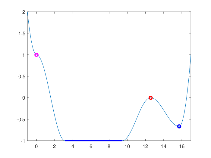
In our simulations, we first numerically verify that converges almost surely to a stationary point of , denoted by . Then we analyse more specifically how is approximated by , ideally in such a way that there exists such that for all . In particular, we run experiments considering different settings for the sequences , and appearing in Assumption 3.
IV-A Experiments under
In this section we investigate the case where the only non-zero sequence (except for the stepsize) interfering in Assumption 3 is . Such kind of noise assumption is generally considered as a baseline in the literature of stochastic optimization, as it is typically verified for the usual constant stepsize SGD scheme when satisfies the Strong Growth condition [31]. Assumptions 3 i)-iii) are then verified as soon as is a non-increasing sequence. As the latter have to be bounded to fulfill Assumption 3-ii), it thus becomes equivalent to take , for every , to also verify Assumption 3-v).
The approximation sequence is generated empirically so as to satisfy both Assumption 3-iv) and v). Specifically, we set, for every , , where is sampled uniformly in . For the stepsize, we set, for every , such that . Finally, we introduce two different perturbation levels to test the SGD algorithm in particularly extreme cases: a moderate perturbation , and an excessively high perturbation .
| Nature of | ? | ||
|---|---|---|---|
| Saddle point | Yes if | ||
| Saddle point | Yes if | ||
| Global Min | Yes if | ||
| Global Min | Yes | ||
| Global or Local Min | Yes if | ||
| Local Max | No |
Table II shows the behaviour of process considering three different initializations . The first initialization is located on the left of saddle point (see graph of in Figure 1). The second initialization is between the saddle point and the interval of global minimizers. And the last one is in a small neighborhood of the local maximizer , taking . In most scenarios, converges to a stationary point so that remains above its limit. The only tricky case arises for high perturbation level when , which seems to be too close to local maximizer .
IV-B Experiments under
In this section, we no longer impose to be equal to zero. Such a situation is regularly encountered as a first relaxed version of the noise resulting from the Strong Growth condition [31]. One typical situation is when, for , the difference between and follows a Gaussian distribution that remains independent from . We adopt such model to conduct our investigation. More specifically, we choose, for all , . Here, is normally distributed, with zero-mean and standard deviation , and does not depend on process so as to have . Moreover, keeps the same properties as in Section IV-A. In order to easily verify Assumption 3 i)-iii) , we set constant sequences and , equal to and , respectively. In practice, we choose with , and for .
In our simulations, we choose as a moderate level of multiplicative noise, and add as an additive one. Despite the higher complexity of the uncertainty model, we obtain slightly better results as the process is able to escape from saddle or local minimizer in all runs (see Figure 2).
A summary of the behaviour of process under these conditions is reported in Table III.
| Nature of | ? | ||
|---|---|---|---|
| Global Min | Yes if | ||
| Global Min | Yes if | ||
| Global Min | Yes if | ||
| Global Min | Yes if | ||
| Global or Local Min | Yes if | ||
| Global or Local Min | Yes if |

IV-C Experiments for non-zero
Here we consider the more generic case where none of the sequences , nor is equal to .
We suppose that, for every , the second order moment of also possesses a non-zero component relatively to . The most difficult assumption to verify is then Ass. 3-iii), which cannot hold for and constant sequences. One can show that choosing, for every , , , and , for , , , and , is sufficient to fulfill Assumptions 3-i)-iii).
We simulate the approximation sequence , where both and follows a 1-mean uniform distribution between and , respectively, and with .
A summary of the behaviour of process under these conditions is reported in Table IV. The only significant difference of behavior compared with the previous subsection is observed for . In this particular case, numerical errors prevent the algorithm from converging.
| Nature of | ? | ||
|---|---|---|---|
| Global Min | Yes if | ||
| Global Min | Yes if | ||
| Global Min | Yes if | ||
| Non-convergence | Undefined | ||
| Global or Local Min | Yes if | ||
| Global or Local Min | Yes if |
V Conclusion
In this article we introduce a new theoretical framework to study almost sure convergence of SGD schemes, in a non-convex context. We further give numerical illustrations to investigate the behaviour of SGD processes, and the relevancy of the different assumptions necessary to ensure their almost sure convergence. This work is base on the theoretical work we initially conducted in [10], where we introduced a new KL framework to investigate almost sure convergence of stochastic processes, in a smooth but non-convex context.
References
- [1] P.-A. Absil, R. Mahony, and B. Andrews. Convergence of the iterates of descent methods for analytic cost functions. SIAM Journal on Optimization, 16(2):531–547, 2005.
- [2] H. Attouch and J. Bolte. On the convergence of the proximal algorithm for nonsmooth functions involving analytic features. Mathematical Programming, 116:5–16, 2009.
- [3] H. Attouch, J. Bolte, P. Redont, and A. Soubeyran. Proximal alternating minimization and projection methods for nonconvex problems: An approach based on the kurdyka-łojasiewicz inequality. Mathematics of Operations Research, 35(2):438–457, 2010.
- [4] D. P. Bertsekas and J. N. Tsitsiklis. Gradient convergence in gradient methods with errors. SIAM Journal on Optimization, 10(3):627–642, 2000.
- [5] J. Bolte, A. Daniilidis, and A. Lewis. The łojasiewicz inequality for nonsmooth subanalytic functions with applications to subgradient dynamical systems. SIAM Journal on Optimization, 17(4):1205–1223, 2007.
- [6] J. Bolte, S. Sabach, and M. Teboulle. Proximal alternating linearized minimization for nonconvex and nonsmooth problems. Mathematical Programming, 146(1-2):459–494, 2014.
- [7] L. Bottou, F. E. Curtis, and J. Nocedal. Optimization methods for large-scale machine learning. SIAM Review, 60(2):223–311, 2018.
- [8] C. Castera, J. Bolte, C. Févotte, and E. Pauwels. Second-order step-size tuning of SGD for non-convex optimization. Neural Processing Letters, 54(3):1727–1752, 2022.
- [9] E. Chouzenoux and J.-B. Fest. SABRINA: A stochastic subspace majorization-minimization algorithm. Journal of Optimization Theory and Applications, 195:919–952, 2022.
- [10] E. Chouzenoux, J.-B. Fest, and A. Repetti. A kurdyka-lojasiewicz property for stochastic optimization algorithms in a non-convex setting. Technical report, 2023. https://arxiv.org/abs/2302.06447.
- [11] E. Chouzenoux, J.-C. Pesquet, and A. Repetti. Variable metric forward–backward algorithm for minimizing the sum of a differentiable function and a convex function. Journal of Optimization Theory and Applications, 162(1):107–132, 2014.
- [12] E. Chouzenoux, J.-C. Pesquet, and A. Repetti. A block coordinate variable metric forward–backward algorithm. Journal of Global Optimization, 66(3):457–485, 2016.
- [13] P. L. Combettes and J.-C. Pesquet. Stochastic forward-backward and primal-dual approximation algorithms with application to online image restoration. In Proceedings of the 24th European Signal Processing Conference (EUSIPCO 2016), pages 1813–1817, 2016.
- [14] A. Defazio, F. Bach, and S. Lacoste-Julien. SAGA: a fast incremental gradient method with support for non-strongly convex composite objectives. Advances in Neural Information Processing Systems, 27, 2014.
- [15] A. Defazio, J. Domke, et al. Finito: A faster, permutable incremental gradient method for big data problems. In Proceedings of the International Conference on Machine Learning (ICML 2014), pages 1125–1133, 2014.
- [16] J. Duchi, E. Hazan, and Y. Singer. Adaptive subgradient methods for online learning and stochastic optimization. Journal of Machine Learning Research, 12(7), 2011.
- [17] S. Gadat. Stochastic optimization algorithms, non asymptotic and asymptotic behaviour. Lecture Notes, University of Toulouse, 2017. https://perso.math.univ-toulouse.fr/m2r/files/2016/02/B5-2016-2017-new.pdf.
- [18] C. Jin, R. Ge, P. Netrapalli, S. M. Kakade, and M. I. Jordan. How to escape saddle points efficiently. In Proceedings of the International Conference on Machine Learning (ICML 2017), pages 1724–1732. PMLR, 2017.
- [19] R. Johnson and T. Zhang. Accelerating stochastic gradient descent using predictive variance reduction. Advances in Neural Information Processing Systems, 26, 2013.
- [20] A. Khaled and P. Richtárik. Better theory for SGD in the nonconvex world. Technical report, 2020. https://arxiv.org/abs/2002.03329.
- [21] D. P. Kingma and J. Ba. Adam: A method for stochastic optimization. Technical report, 2014. https://arxiv.org/abs/1412.6980.
- [22] K. Kurdyka. On gradients of functions definable in o-minimal structures. In Annales de l’Institut Fourier, volume 48, pages 769–783, 1998.
- [23] S. Lojasiewicz. Une propriété topologique des sous-ensembles analytiques réels. Les équations aux dérivées partielles, 117:87–89, 1963.
- [24] S. Y. Meng. Stochastic second-order optimization for over-parameterized machine learning models. PhD thesis, University of British Columbia, 2020.
- [25] J. Nocedal and S. J. Wright. Numerical Optimization. Springer, 1999.
- [26] A. Repetti and Y. Wiaux. Variable metric forward-backward algorithm for composite minimization problems. SIAM Journal on Optimization, 31(2):1215–1241, 2021.
- [27] H. Robbins and S. Monro. A stochastic approximation method. The Annals of Mathematical Statistics, pages 400–407, 1951.
- [28] H. Robbins and D. Siegmund. A convergence theorem for non negative almost supermartingales and some applications. In Optimizing Methods in Statistics, pages 233–257. 1971.
- [29] N. Roux, M. Schmidt, and F. Bach. A stochastic gradient method with an exponential convergence rate for finite training sets. Advances in Neural Information Processing Systems, 25, 2012.
- [30] K. A. Sankararaman, S. De, Z. Xu, W. R. Huang, and T. Goldstein. The impact of neural network overparameterization on gradient confusion and stochastic gradient descent. In Proceedings of the International Conference on Machine Learning (ICML 2020), pages 8469–8479. PMLR, 2020.
- [31] M. Schmidt and N. L. Roux. Fast convergence of stochastic gradient descent under a strong growth condition. Technical report, 2013. https://arxiv.org/abs/1308.6370.
- [32] T. Tieleman, G. Hinton, et al. Lecture 6.5-rmsprop: Divide the gradient by a running average of its recent magnitude. COURSERA: Neural Networks for Machine Learning, 4(2):26–31, 2012.
- [33] S. Vaswani, F. Bach, and M. Schmidt. Fast and faster convergence of SGD for over-parameterized models and an accelerated perceptron. In Proceedings of the 22nd International Conference on Artificial Intelligence and Statistics (AISTATS 2019), pages 1195–1204. PMLR, 2019.
- [34] X. Wang, S. Ma, D. Goldfarb, and W. Liu. Stochastic quasi-Newton methods for nonconvex stochastic optimization. SIAM Journal on Optimization, 27(2):927–956, 2017.
