Optimization of Speed and Network Deployment for Reliable V2I Communication in the Presence of Handoffs and Interference

Vehicle-to-infrastructure (V2I) communication is pivotal to enable autonomous and well-informed decision-making in connected and autonomous vehicles (CAVs); thus, improving road safety and traffic flow [1]. Nevertheless, optimizing the speed of CAVs while maximizing the CAV traffic flow and achieving reliable connectivity at the same time is challenging. The reason is that while increasing the CAVs’ speed improves the traffic flow, it also increases communication handoffs (HOs) as the CAVs switch from one base-station (BS) to another, thus reducing data rates. Furthermore, unplanned deployment of network infrastructure such as roadside units or BSs may result in severe interference which negatively impacts CAV data rate [2]. A fundamental trade-off thus exists between the communication data rates and CAV traffic flow. In this context, this letter aims to answer the following questions, i.e., (i) how to analyze the performance of V2I communication considering HOs and interference? and (ii) what is the optimal BS density and average CAV speed that maximize traffic flow?

Prior research works in the realm of V2I communications have considered mobility in terms of data rates, however traffic flow is typically overlooked. For instance, in [3], Arshad et al. derived HO-aware data rates as a function of the speed of the user device and the HO cost from the BSs. In [2], Hossan et al. presented a stochastic geometry framework to derive the HO-aware coverage probability of a two-tier wireless network with RF and THz BSs. In [4], Lin et al. proposed a random way-point mobility model to characterize the HO rate and sojourn time using stochastic geometry considering randomly distributed BSs. Recently, in [5], Yan et al. proposed a reinforcement learning approach for joint V2I network selection and autonomous driving policies considering both RF and THz BSs. Their results demonstrated inter-dependency of a CAV’s motion dynamics, HOs, and data rate to adopt safe driving behaviours for CAVs.

Another series of research contributions characterizes traffic flow using macroscopic models [6, 7], however V2I communications is typically overlooked.

None of the aforementioned research works considered the problem of CAVs traffic flow maximization with log-normally distributed CAVs’ spacing and HO-aware data rate constraints in a large-scale interference-limited wireless network. To this end, our contributions can be summarized as follows:

$\bullet$ We characterize macroscopic traffic flow by considering log-normal distribution of the spacing between CAVs. We then derive novel and tractable closed-form expressions for the probability density function (PDF) and cumulative density function (CDF) of signal-to-interference-plus-noise ratio (SINR), HO-aware rate outage probability and ergodic capacity in a large-scale network with interference. The derived expressions capture the network parameters such as height of the BSs, safety distance of BSs from the road, interference from neighboring BSs, and channel fading.

$\bullet$ We develop a novel optimization framework to jointly optimize the deployment density of the BSs and speed of CAVs to maximize the CAVs’ traffic flow with collision avoidance and minimum HO-aware data rate constraints.

$\bullet$ Numerical results confirm the accuracy of the derived expressions and extract useful insights related to dynamics of BS density, CAV minimum data rate requirements, average CAV speed, BS heights and safety distances, etc.

We consider a road of length $L_{R}$ on which $N_{c}$ CAVs travel. We consider $N$ BSs are deployed alongside the road at a certain distance $d_{\mathrm{safe}}$ with a density defined as the number of BSs deployed per unit distance, i.e., $\mu=N/L_{R}$. The distance between BSs is $1/\mu$ as shown in Fig. 1. The CAVs’ density $k$ on the road is defined as the number of CAVs per unit distance, and the CAVs’ speed is $v$. According to macroscopic traffic flow theory, the flow of vehicles is defined as $q=kv$ vehicles per unit time [8]. Note that $k$ is inversely proportional to $s$, i.e., $k=1/s$ and $s$ is the spacing between neighboring vehicles. Given the PDF of the density of vehicles $k$ on the road $f_{K}(k)$, the traffic flow can be defined as follows:

In this paper, we model the inter-vehicle spacing $s$ with a log-normal distribution. This model has been proven to be accurate for daytime hours through various empirical studies [9]. The research works observed the traffic flow behaviour during different times of the day, and proved that the inter-vehicle spacing distribution is log-normally distributed during day-time hours (i.e., moderate traffic). Therefore, we consider the inter-vehicle spacing $s$ to be log-normally distributed during day-time hours with PDF given as:

where $\mu_{\mathrm{LN}}$ and $\sigma_{\mathrm{LN}}$ are the logarithmic average and scatter parameters of log-normal distribution, respectively, and erf($\cdot$) is the error function. Therefore, (1) can be rewritten as follows:

Each CAV is assumed to be connected to a single nearest BS at any given time. Considering the distance-based path-loss and short-term multi-path fading at the transmission channel, the received signal power at a given CAV $i$ from a given BS $j$ in the downlink can be modeled as follows:

The signal-to-interference-plus noise ratio (SINR) received at a $i$-th CAV from $j$-th BS can thus be modeled as follows:

where $G_{R}^{\mathrm{tx}}$ and $G_{R}^{\mathrm{rx}}$ represent the transmitting and receiving antenna gains, respectively, $P_{j}^{\mathrm{tx}}$ represents the transmit power of the BS $j$, $\chi_{i,j}$ represents the short-term channel fading of BS $j$ modeled with Rayleigh distribution, $c$ and $f_{R}$ represent the speed of an electromagnetic wave and RF carrier frequency, respectively, $d_{i,j}$ represents the distance between the $j$-th BS and $i$-th CAV, and $\alpha$ represents the path-loss exponent. Furthermore, $N_{R}$ is the thermal noise power at the receiver and $I_{i}=\sum_{k\neq j}P_{k}^{\mathrm{tx}}\gamma_{R}d^{-\alpha}_{i,k}\chi_{i,k}$ is the cumulative interference at the $i$-th CAV from the interfering BSs, where $\gamma_{R}=G_{R}^{\mathrm{tx}}G_{R}^{\mathrm{rx}}(c/4\pi f_{R})^{2}$, $d_{i,k}$ represents the distance between the $i$-th CAV and $k$-th interfering BS, and $\chi_{i,k}$ is the power of fading from the $k$-th interfering BS to the CAV.

Furthermore, as detailed in Fig. 1, the distance between a CAV $i$ and BS $j$ can be calculated using their respective coordinates as $d_{i,j}=\sqrt{x_{i,j}^{2}+h_{\mathrm{bs}}^{2}+d_{\mathrm{safe}}^{2}},$ where $h_{\mathrm{bs}}$ represents the height of the BSs, $d_{\mathrm{safe}}$ represents the safety distance from the CAV on the road to the BS, and $x_{i,j}$ is the distance parallel to the road with respect to the location of the CAV on the road to the BS. Subsequently, given the Shannon-Hartley theorem for infinite block-length regime, the data rate without mobility between a BS and CAV can be defined as $R_{i,j}=W\log_{2}(1+\text{SINR}_{i,j})$ where $W$ represents the bandwidth of the channel.

As CAVs drive along the road, HOs between different BSs occur, and due to HO delays and failures, an increase in the rate of HOs can negatively impact the CAV data rate. Therefore, we incorporate the effect of these HOs through the HO-related cost. HO cost is proportional to the HO delay ($h_{d}$) measured in seconds per HO, and HO rate ($H$) measured in number of HOs per second, i.e., $H_{c}=h_{d}\times H.$ Since we assume nearest BS association for CAVs, we define $H$ as the number of cell boundaries a CAV crosses per second, where a cell boundary is the coverage range of a BS. Note that the number of boundaries per unit distance are the same as the BS density $\mu$. By using the speed of CAVs $v$, we can calculate the number of boundaries covered by a CAV per second as $H=\mu v$. Thus, we model the HO-aware data rate [3] as:

where $H_{c,\text{max}}=h_{d}\frac{H}{\mu_{\text{max}}V_{\text{max}}}=h_{d}\frac{\mu v}{\mu_{\text{max}}V_{\text{max}}}$ is the normalized HO cost in equation (5) to ensure $0\leq H_{c,\text{max}}<1$, $\mu_{\text{max}}$ is the maximum regulated BS density, and $V_{\text{max}}$ is the maximum regulated speed of the CAVs. Finally, a stable CAV connection with the nearest BS requires a minimum HO-aware data rate $R_{\text{th}}$ which ensures that every CAV achieves the required QoS.

In this section, we derive novel closed-form expressions for the PDF and CDF of SINR, HO-aware rate outage probability, as well as the ergodic HO-aware data rate. The HO-aware rate outage probability $P_{\mathrm{out}}$ is defined as:

where $\gamma_{\mathrm{th}}$ is the desired SINR threshold given as $\gamma_{\mathrm{th}}=2^{\frac{R_{\mathrm{th}}}{W(1-H_{c,\mathrm{max}})}}$ and $H_{c,\mathrm{max}}=h_{d}\frac{\mu v}{\mu_{\mathrm{max}}V_{\mathrm{max}}}$. The outage expression can then be derived as shown in the following lemma.

In the following, we characterize the average HO-aware data rate using the statistics of SINR.

To simplify the optimization, we also provide a worst-case bound on the interference.

In this section, we formulate the macroscopic traffic flow maximization problem with various constraints to jointly optimize the CAV speed $v$ and the BS density $\mu$ in the presence of interference. Note that BS density optimization can also be implemented in practice by dynamically switching the BSs. We present a closed-form expression for the optimal CAV speed and a numerical method to compute optimal $\mu$. The traffic flow maximization problem is formulated as:

where C1 is the collision avoidance constraint which ensures that the speed of the CAVs should not exceed $s/\tau$, i.e.,

where $s$ is the distance between two CAVs and is always greater than zero, $\tau$ represents the processing time for the CAVs to act on a decision, and $\epsilon$ is the crash tolerance level. In addition, equation (16) can be rewritten by substituting the CDF of $s$ where $\mathrm{\mathrm{Pr}}\left(v\geq\frac{s}{\tau}\right)=\frac{1}{2}\left(1+\mathrm{erf}\left(\frac{\ln{(v\tau)}-\mu_{\mathrm{LN}}}{\sigma_{\mathrm{LN}}\sqrt{2}}\right)\right)$. By using the inverse error function and taking the inverse log of both sides and factoring for $v$, (16) can be rewritten as in C1. C1 indicates that speed is capped to create an adequate safety distance that is traversed during the processing time. We refer to the right side of C1 as the maximum safe speed that keeps the crash probability below $\epsilon$. The condition C1 shows that the maximum safe speed increases with $\epsilon$, but decreases with the processing time.

Furthermore, C2 is the worst-case HO-aware data rate constraint of the CAV based on Lemma 3, i.e.,

By factoring out for $v$ we can rewrite (17) as in C2, where we refer to the right side of C2 as the maximum speed, denoted by $V_{\textrm{data}}(\mu)$ that ensures the minimum data rate requirement of the CAVs. To ensure that C2 does not attain negative values of speed and the problem remains feasible, we introduce the constraint C3. That is, C3 ensures $\frac{R_{\text{th}}}{WR_{\mathrm{worst}}(\mu)}\leq 1$. The final two constraints C4 and C5 cap the speed and BS density to a maximum, respectively. Note that problem P1 is a non-linear programming problem due to constraints C2 and C3 which are a non-linear function of $\mu$. To solve this problem, we first compute the optimal speed $v^{*}$ which is then further maximized to optimize BS density as in the following Lemma.

It is important to note that due to the interference expression and its dependency on BS density, there is no closed-form expression for $\mu^{*}$. Therefore, we utilize one-dimensional numerical optimization techniques to solve for $\mu^{*}$.

Finally, by substituting (18) and $\mu^{*}$ into the objective function of P1, we derive the optimal traffic flow as follows:

In this section, we validate the accuracy of the derived expressions through computer simulations. Furthermore, we demonstrate the sensitivity of optimal traffic flow by changing key parameters such as crash tolerance level, data rate thresholds, interference, etc. Unless stated otherwise, the values of the system parameters [2] are used in the following figures are listed herein. $V_{\mathrm{max}}=30$ m/s, $\mu_{\mathrm{max}}=0.01$ BSs/m, $h_{d}=3$ s/HO, $R_{\mathrm{th}}=60$ Mbps, $W=40$ MHz, $G_{R}^{\mathrm{tx}}=1$ dB, $G_{R}^{\mathrm{rx}}=1$ dB, $c=3\times 10^{8}$ m/s, $f_{R}=2.1$ GHz, $N_{R}=1.507\times 10^{-13}$ W/$\mathrm{m}^{2}$, $P_{j}^{\mathrm{tx}}=1$ W, $\alpha=3$, $\lambda=1$, $\epsilon=1\%$, $\tau=6\times 10^{-3}$ sec, $\mu_{\mathrm{LN}}=0$, $\sigma_{\mathrm{LN}}=1$, $d_{\mathrm{safe}}=5$ m, $h_{\mathrm{bs}}=8$ m, $L_{R}=2000$ m.

Fig. 4 and Fig. 4 demonstrate the outage probability (7) and ergodic capacity (15) as a function of $\mu$ for various CAV speeds. The analytical expression match perfectly with the simulation results. When $\mu$ increases, the outage increases and rate decreases due to increasing interference and HOs. Furthermore, higher speeds result in higher probability of outage and lower ergodic capacity when compared to lower speeds, which is due to more frequent HOs.

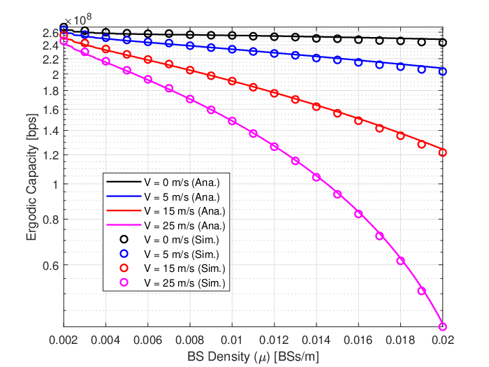
Fig. 4 depicts $V_{\mathrm{data}}$ as a function of $\mu$. As $\mu$ increases, $V_{\mathrm{data}}$ with $\alpha=3$ increases up to a certain point due to vicinity of BSs. However, beyond that point $V_{\mathrm{data}}$ begins to decrease due to an increase in HOs and interference, and the CAVs need to lower their speed. On the other hand, when $\alpha=4$, the benefit of rate enhancement cannot be seen and a higher $\mu$ only causes more interference and HOs. Furthermore, we show that different CAV processing times $\tau$ varies $V_{\mathrm{safe}}$, where $v^{*}=V_{\mathrm{safe}}$ for higher $\tau$ values when $V_{\mathrm{safe}}<V_{\mathrm{data}}$.

Fig. 7 depicts the impact of the data rate threshold $R_{\mathrm{th}}$ on traffic flow $Q$ and the optimal BS density $\mu^{*}$ for various path-loss exponents. As seen on the top of Fig. 7, as $R_{\mathrm{th}}$ increases, $Q$ decreases as CAVs need to reduce their speed to limit the number of HOs to meet the required data rate. For the same reason, when $R_{\mathrm{th}}$, $\mu^{*}$ increases. The environments with higher path-loss exponents require more dense BS deployment. Note that we consider 100 points (or $R_{\mathrm{th}}$ values) along the x-axis between $6\times 10^{7}$ bps and $8\times 10^{7}$ bps to compute analytical traffic flow which requires to compute the optimal density of BSs $\mu^{*}$ numerically using MATLAB’s fminbnd function at each $R_{\mathrm{th}}$ value. Therefore, minor fluctuations are observed due to numerical computations of $\mu^{*}$.

Fig. 7 depicts the relationship between the crash tolerance level $\epsilon$ and optimum traffic flow $Q$ for various CAV processing times. At first, $V_{\mathrm{safe}}<V_{\mathrm{data}}<V_{\mathrm{max}}$, thus the optimal speed is bound to $V_{\mathrm{safe}}$ as in Lemma 4, where $V_{\mathrm{safe}}$ increases as the crash intensity level $\epsilon$ increases since we are relaxing the crash tolerance. After a certain $\epsilon$ value, $V_{\mathrm{safe}}>V_{\mathrm{data}}$. The optimal speed is bound to $V_{\mathrm{data}}$ as in Lemma 4, which is constant with respect to $\epsilon$ and results in an upbound flat curve. For different CAV processing times $\tau$, the point at which $V_{\mathrm{data}}$ takes over changes. When the CAV processing time is larger, $V_{\mathrm{safe}}$ is smaller since it takes a longer time for the CAV to process decisions compared to smaller $\tau$ values.

Finally, Fig 7 depicts the relationship between BS density $\mu$ and traffic flow $Q$ with various BS safety distances. At first, when the BS density $\mu$ is lower, $V_{\mathrm{safe}}<V_{\mathrm{data}}<V_{\mathrm{max}}$ so the optimal speed is bound to $V_{\mathrm{safe}}$ as in Lemma 4. $V_{\mathrm{safe}}$ is constant with respect to $\mu$ which results in an upbound flat curve. As $\mu$ increases, HOs and interference increases which lowers $V_{\mathrm{data}}$ to the point where $V_{\mathrm{safe}}>V_{\mathrm{data}}$ and the optimal speed is bound to $V_{\mathrm{data}}$ as in Lemma 4. For different BS safety distances $d_{\mathrm{safe}}$, the switching point between $V_{\mathrm{safe}}$ and $V_{\mathrm{data}}$ changes because the further away the BS is from the CAV, $V_{\mathrm{data}}$ will decrease because of weak signal strength. Furthermore, the traffic flow without interference results in better traffic flow as compared to the traffic flow with interference as the interference deteriorates the data rate, CAV speed, and traffic flow.

This letter presents a framework for V2I communications for CAVs where we derive novel expressions for outage probability and ergodic capacity of HO-aware data rate, and jointly optimize the speed and network deployment in the presence of HOs between BSs and interference due to neighbouring BSs. Finally, we demonstrate the trade-off between achievable wireless data rates and traffic flow.

References

- [1] L. Hobert, A. Festag, I. Llatser, L. Altomare, F. Visintainer, and A. Kovacs, “Enhancements of V2X communication in support of cooperative autonomous driving,” IEEE Commun. Magazine, vol. 53, no. 12, pp. 64–70, 2015.
- [2] M. T. Hossan and H. Tabassum, “Mobility-aware performance in hybrid RF and Terahertz wireless networks,” IEEE Trans. on Commun., vol. 70, no. 2, pp. 1376–1390, 2022.
- [3] R. Arshad, H. ElSawy, S. Sorour, T. Y. Al-Naffouri, and M.-S. Alouini, “Velocity-aware handover management in two-tier cellular networks,” IEEE Trans. on Wireless Commun., vol. 16, no. 3, pp. 1851–1867, 2017.
- [4] X. Lin, R. K. Ganti, P. J. Fleming, and J. G. Andrews, “Towards understanding the fundamentals of mobility in cellular networks,” IEEE Trans. on Wireless Commun., vol. 12, no. 4, pp. 1686–1698, 2013.
- [5] Z. Yan and H. Tabassum, “Reinforcement learning for joint V2I network selection and autonomous driving policies,” in IEEE Global Commun. Conference, 2022, pp. 1241–1246.
- [6] J. Popping, E. Begeleider, and T. Begeleider, “An overview of microscopic and macroscopic traffic models,” 2013.
- [7] X. Shi and X. Li, “Constructing a fundamental diagram for traffic flow with automated vehicles: Methodology and demonstration,” Transportation Research Part B: Methodological, vol. 150, pp. 279–292, 2021.
- [8] R. Mahnke, J. Kaupužs, and I. Lubashevsky, “Probabilistic description of traffic flow,” Physics Reports, vol. 408, no. 1, pp. 1–130, 2005.
- [9] N. Wisitpongphan, F. Bai, P. Mudalige, V. Sadekar, and O. Tonguz, “Routing in sparse vehicular ad hoc wireless networks,” IEEE Journal on Selected Areas in Commun., vol. 25, no. 8, pp. 1538–1556, 2007.
- [10] S. Khaled, T. Kadri, and S. Kadry, “Hypoexponential distribution with different parameters,” Journal of Applied Mathematics, vol. 4, pp. 624–631, 04 2013.
- [11] N. Jawad, A. Nasar, and J. Hadad, “Distributions of the ratio and product of two independent weibull and lindley random variables,” Journal of Probability and Statistics, vol. 2020, 05 2020.
- [12] M. Monemi and H. Tabassum, “Performance of UAV-assisted D2D networks in the finite block-length regime,” IEEE Trans. on Commun., vol. 68, no. 11, pp. 7270–7285, 2020.
- [13] W. H. Press, S. A. Teukolsky, W. T. Vetterling, and B. P. Flannery, Numerical Recipes 3rd Edition: The Art of Scientific Computing, 3rd ed. USA: Cambridge University Press, 2007.
- [14] “Chapter 11 - basic methods,” in Numerical Methods and Optimization in Finance (Second Edition), second edition ed., M. Gilli, D. Maringer, and E. Schumann, Eds. Academic Press, 2019, pp. 229–271.
- [15] D. E. Ferguson, “Fibonaccian searching,” Commun. ACM, vol. 3, no. 12, p. 648, 1960.