跳到论文正文
W Papers独立论文阅读器 arXiv:2307.06739 论文正文 计算阅读时间 · 0%
引用这篇论文根据当前论文元数据生成,正式投稿前建议核对。


License: CC BY 4.0
arXiv:2307.06739v2 [math.ST] 25 Jul 2023

A zero-estimator approach for estimating the signal level in a high-dimensional regression setting

Ilan Livne

A zero-estimator approach for estimating the signal level in a high-dimensional regression setting

Research Thesis

In Partial Fulfillment of the Requirements for the Degree of Doctor of Philosophy

Ilan Livne

Submitted to the Senate of the Technion - Israel Institute of Technology

Tishrei, 5783, Haifa, September, 2022

\justify

The research thesis was done under the supervision of Dr. David Azriel and Prof. Yair Goldberg in the Faculty of Industrial Engineering and Management.

The author of this thesis states that the research, including the collection, processing and presentation of data, addressing and comparing to previous research, etc., was done entirely in an honest way, as expected from scientific research that is conducted according to the ethical standards of the academic world. Also, reporting the research and its results in this thesis was done in an honest and complete manner, according to the same standards.

Publications in peer-reviewed journals

The paper “Improved Estimators for Semi-supervised High-dimensional Regression Model” has been recently published in the Electronic Journal of Statistics.
The paper “A zero-estimator approach for estimating the signal level in a high-dimensional model-free setting” was submitted to the Journal of Statistical Planning and Inference, and is currently under review.

Conference presentations

Livne, I., Azriel D., Goldberg Y. (2022) Improved Estimators for Semi-supervised High-dimensional Regression Model. The First International Israel Data Science Initiative Conference (IDSI-2022), January 22, Israel.

Acknowledgments

I would like to express my sincere gratitude to my advisors, Dr. David Azriel and Prof. Yair Goldberg, for their guidance throughout my Ph.D period. It has been a long and challenging journey, with many ups and downs, and I am grateful that I had the opportunity to be under their excellent supervision. I can honestly say that I was fortunate to be mentored by two brilliant statisticians, but no less importantly, they are also very kindhearted and supportive. While working with David and Yair, I always felt like their students are their priority despite their many academic responsibilities and busy schedules. I see them as my role models and I feel that I could not have asked for better mentors. Yael and I sometimes joke, during our coffee breaks, about our fear of working for anyone other than Yair or David.

On a more personal note, I want to express my gratitude and appreciation to David for his thorough and insightful responses to all my questions during my PhD studies. Our ongoing email exchanges and Zoom meetings have been a valuable in my learning process. David have helped me to develop a deeper understanding of the nuances of high-quality statistical research. His courses on statistical theory and regression have provided a strong foundation for my specific research and for my overall understanding of statistics. It is an honor to be David’s first PhD student, and I am confident that many more students will benefit from his great mentorship in the future. I am deeply appreciative of his valuable contributions to my academic and professional growth. Thank you David!

Additionally, I wish to express my gratitude to Yair, whose influence on me began even before I started my PhD, while I was still working in London and trying to decide my next career steps. Yair played a significant role in my decision to live in Haifa and study at the Technion (which I am very grateful for). His commitment to my professional training, even while he was extremely busy working on Covid-19 projects during the pandemic, is something I am very grateful for. Furthermore, his influence on me continued even after the PhD as he provided me with guidance and mentorship while I was considered my future career options. A few weeks ago, I started a postdoc position at the Gertner institute, where I can do interesting applied research and develop my skills under the mentorship of some excellent statisticians (including Yair). Thank you Yair for this opportunity, and for your continued support and guidance!

Next, I would like to thank my two committee members (thesis examiners), Paul Feigin and Saharon Rosset, for their valuable input to my thesis. Their comments and corrections have helped me to improve my dissertation and have deepened my understanding of the topic.

In addition to professors, I am fortunate to have received support from several great people in the faculty. Specifically, for computing help, I am grateful to Efrat Maimon for her help in setting up the cloud server that enables me to run my simulations. I also grateful to Vadim Derkach and David Miller for their technical support. Without their assistance, I would not have been able to complete my PhD successfully.

Many thanks belong my colleagues and friends who have supported me throughout my PhD period. I especially want to thank Yael Travis-Lumer and Tiantian Liu for consistently being a supportive presence, offering a listening ear and valuable insights. The friendship with Yael and Tiantian has not only contributed to my statistical knowledge, but it has also been valuable in helping me navigate the ups and downs that come with doing a PhD. Thank you Yael and Tiantian!

I also want to thank my friend and excellent ping-pong partner, Ofra Amir, for her support throughout my PhD journey. Ofra was especially helpful during times when my research was experiencing obstacles, offering valuable tips and advice that helped me to maintain a positive mindset that was needed to overcome these challenges. I will leave the Technion with many good memories of crazy ping-pong matches, chocolate breaks, and deep conversations while enjoying the beautiful view from the roof of the faculty building. Thank you Ofra for your support and friendship!

It is no secret that I had a rough start to my PhD program. A few weeks after starting, I developed Ramsay Hunt Syndrome, a rare complication of shingles that affects the facial nerve and causes facial paralysis. I could not close or blink my eye, and I suffered from tinnitus, severe eye pain and nerve pains. These symptoms made it impossible for me work and focus on my PhD research and it took me many months until I was able to work properly again. Additionally, during my PhD studies, I had to undergo three different surgeries to reduce the chronic facial pain that I was left with due to a poor recovery from Ramsay Hunt Syndrome. Despite my illness, I was fortunate to receive the monthly scholarship from the Technion throughout the entire time. I will always be grateful for this, as it was heartwarming to know the Technion allowed me to take the time I needed to get back on my feet and continue my PhD journey without flunking. The generous financial help of the Technion is gratefully acknowledged.

I would like to thank my father, who is no longer with us, for inspiring my love for science and math and for teaching me the importance of determination and perseverance in the face of challenges. I am also grateful to my mother, who took care of me during the early stages of my PhD, when I was battling the severe symptoms of Ramsay Hunt Syndrome. I cannot possibly thank her enough for her support and care during that time. Finally, I would like to thank my two baby twins, Guy and Daniel, who taught me the joy and meaning of being a father through many sleepless nights. And most of all, I would like to thank my wife and lifelong partner, Merav, who has always believed in and supported me. Without her constant help and support, I don’t know where I would be today.

Abstract

We study a high-dimensional linear regression model in a semi-supervised setting, where for many observations only the vector of covariates XX is given with no responses YY. We do not make any sparsity assumptions on the vector of coefficients, nor do we assume normality of the covariates. We aim at estimating the signal level, i.e., the amount of variation in the response that can be explained by the set of covariates. We propose an estimator, which is unbiased, consistent, and asymptotically normal. This estimator can be improved by adding zero-estimators arising from the unlabeled data. Adding zero-estimators does not affect the bias and potentially can reduce the variance. We further present an algorithm based on our approach that improves any given signal level estimator. Our theoretical results are demonstrated in a simulation study.

Key words and phrases: Linear Regression, Semi-supervised setting, U-statistics, Variance estimation, Zero estimators.

Abstract

We study a high-dimensional regression setting under the assumption of known covariate distribution. We aim at estimating the amount of explained variation in the response by the best linear function of the covariates (the signal level). In our setting, neither sparsity of the coefficient vector, nor normality of the covariates or linearity of the conditional expectation are assumed. We present an unbiased and consistent estimator and then improve it by using a zero-estimator approach, where a zero-estimator is a statistic whose expected value is zero. More generally, we present an algorithm based on the zero estimator approach that in principle can improve any given estimator. We study some asymptotic properties of the proposed estimators and demonstrate their finite sample performance in a simulation study.

Key words and phrases: Linear Projection, Semi-supervised setting, U-statistics, Variance estimation, Zero-estimators.

List of Abbreviations and Notation

Abbreviations

MSE Mean Squared Error
RMSE Root Mean Squared Error
OLS Ordinary Least Squares
GWAS Genome Wide Association Studies
UMVUE Uniformly Minimum-Variance Unbiased Estimator
OOE Optimal Oracle Estimator

Notation

XX The vector of covariates
YY The response variable
τ2\tau^{2} The signal level, i.,e the variance that is explained by the model
σ2\sigma^{2} The noise level, i.,e the variance that is left unexplained by the model
X The n×pn\times p design matrix
Y The n×1n\times 1 vector of responses
𝚺{\bf\Sigma} The p×pp\times p covariance matrix of the covariates
‖A‖F2\|\textbf{A}\|_{F}^{2} The Frobenius norm of matrix A
δ\delta A covariate-selection procedure
𝐒δ{\bf S}_{\delta} The selected subset of indices by the covariate-selection procedure δ\delta

Abstract

\justify

Analysis of high-dimensional data, where the number of covariates is larger than the sample size, is a topic of current interest. In such settings, an important goal is to estimate the signal level τ2\tau^{2} and noise level σ2\sigma^{2}, i.e., to quantify how much variation in the response variable can be explained by the covariates, versus how much of the variation is left unexplained. This thesis considers the estimation of these quantities in a semi-supervised setting, where for many observations only the vector of covariates XX is given with no responses YY. That is, the data contain two parts, in the first part both the covariates and the responses are given (labeled data) and in the second part, only the covariates are given (unlabeled data). Our main research question is: “how can one use the unlabeled data to better estimate τ2\tau^{2} and σ2\sigma^{2}?”

We consider two frameworks: a linear regression model and a linear projection model in which linearity is not assumed. In the first framework, while the linear regression model is used, no sparsity assumptions on the coefficients are made. In the second framework, the linearity assumption is also relaxed and we aim to estimate the signal and noise levels defined by the linear projection.

We first propose a naive estimator which is unbiased and consistent, under some assumptions, in both frameworks. We then show how the naive estimator can be improved by using zero-estimators, where a zero-estimator is a statistic arising from the unlabeled data, whose expected value is zero. Adding a zero-estimator does not affect the bias and potentially can reduce the variance. In the first framework, we were able to calculate the optimal zero-estimator improvement and discuss ways to approximate the optimal improvement. In the second framework, such optimality does no longer hold and we suggest two zero-estimators that improve the naive estimator although not necessarily optimally. Furthermore, we show that the zero-estimator approach reduces the variance for general initial estimators and we present an algorithm that potentially improves any initial estimator. This holds in both frameworks.

Lastly, we consider four datasets and study the performance of our suggested methods. We found that by using our methods, we were able to improve for the naive and another estimator (EigenPrism) in all these datasets.

1 Introduction

In many regression settings, an important goal is to estimate the signal level τ2\tau^{2} and the noise level σ2\sigma^{2}, i.e., to quantify how much variation in the response variable can be explained by the covariates, versus how much of the variation is left unexplained. For example, methods that aim at performing inference on individual coefficients in a high-dimensional setting, where the number of covariates is larger than the sample size, typically require knowledge of σ2\sigma^{2}; see Berk et al. 2013 and references therein. Beyond regression coefficient inference, the signal and noise levels play also an important role in various statistical applications including regression diagnostics, prediction accuracy, and model selection procedures such as AIC and BIC. Both τ2\tau^{2} and σ2\sigma^{2} are also closely related to other important concepts such as genetic heritability, signal-to-noise ratio, and signal detection (Visscher et al. 2008).

When the covariates’ dimension is low and a linear regression model is assumed, the ordinary least squares method can be used to find consistent estimators. However, in a high-dimensional setting the least squares method breaks down and it becomes more challenging to develop good estimators without further assumptions. In recent years, several fruitful methods have been proposed for estimating the signal level under the assumption that the regression coefficient vector β\beta is sparse or has some probabilistic structure (e.g., β\beta is Gaussian) (Fan et al. 2012, Sun and Zhang 2012, Verzelen et al. 2018, Yang et al. 2010). In addition, rather than assuming sparsity or other structural assumptions on β\beta, a different direction for estimating the signal and noise levels in a high-dimensional setting was to assume strong distributional assumptions on the covariates, such as independent Gaussian structure (Dicker 2014, Janson et al. 2017). However, methods that rely on specific assumptions on β\beta, or on the distribution of the covariates may not perform well when these assumptions fail to hold.

Motivated to relax the above assumptions, we consider the estimation of τ2\tau^{2} and σ2\sigma^{2} in a semi-supervised setting. Here, a semi-supervised setting is a setting in which a large amount of unlabeled data is available. Such a setting arises, for example, when the covariates XX are easily measured but the responses YY are more difficult or expensive to collect. In general, the purpose of a semi-supervised technique is to incorporate the additional information that is available in the unlabeled data to improve the inference of the parameters of interest. Our main research question is: “how can one use the unlabeled data to better estimate τ2\tau^{2} and σ2\sigma^{2}?”

We consider two high-dimensional regression frameworks: a linear regression model and a linear projection model, in which linearity is not assumed. In the first framework, where the linear regression model is used, no sparsity assumptions on the coefficients are made. In the second framework, the linearity assumption is also relaxed and we aim to estimate the signal and noise levels defined by the linear projection. In general, we do not assume Gaussian covariates for developing our theoretical result, but in a few cases we use this assumption to obtain stronger results.

We begin by proposing a naive estimator for the signal level τ2\tau^{2}, which is unbiased and consistent under some assumptions, in both frameworks. We then show how the naive estimator can be improved by adding zero-estimators, where a zero-estimator is a statistic arising from the unlabeled data, whose expected value is zero. Adding zero-estimators to an initial estimator does not affect its bias and potentially can reduce its variance (Bahadur 1957, Lehmann and Casella 1998b).

The rest of this work is organized as follows. Chapter 2 is based on a manuscript that was submitted after revision to the Electronic Journal of Statistics. In this chapter, we consider the linear regression framework and present the naive estimator and study ways to improve it by the zero-estimator approach. We find the optimal zero-estimator improvement with respect to linear families of zero-estimators. The optimal improvement generally cannot be achieved since it depends on the unknown parameters and we suggest two methods to approximate the optimal improvement. We further study the theoretical properties of our suggested estimators and also provide an algorithm that generalizes our method to improve other estimators of the signal level τ2\tau^{2}.

Chapter 3 is based on a manuscript that was submitted to the Journal of Statistical Planning and Inference. This chapter presents a modification of our methods to the linear projection framework where linearity is not assumed. Here, the naive estimator is still unbiased and consistent, under some assumptions, but the above optimal improvement cannot be computed in the same way as in Chapter 2. Nevertheless, we suggest two methods to improve the naive estimator and study their properties. As in Chapter 2, we present a general algorithm that potentially can improve any initial estimator.

In Chapter 4, we apply our suggested estimators to four real datasets and study their performance. We found that by using our methods, we were able to improve for the naive estimator, and the Eigenprism estimator of Janson et al. 2017 for the signal level, in all these datasets. Chapter 5 concludes the thesis with some discussion and directions for future research.

The paper “Improved Estimators for Semi-supervised High-dimensional Regression Model” is submitted to the Electronic Journal of Statistics.

2 Improved Estimators for Semi-supervised High-dimensional Regression Model

2.1 Introduction

High-dimensional data analysis, where the number of predictors is larger than the sample size, is a topic of current interest. In such settings, an important goal is to estimate the signal level τ2\tau^{2} and the noise level σ2\sigma^{2}, i.e., to quantify how much variation in the response variable YY can be explained by the covariates XX, versus how much of the variation is left unexplained. Formally, the variance of YY can be written as Var​[E⁡(Y|X)]+E⁡[Var​(Y|X)]≡τ2+σ2.\text{Var}[E(Y|X)]+E[\text{Var}(Y|X)]\equiv\tau^{2}+\sigma^{2}. For example, in disease classification using DNA microarray data, where the number of potential predictors, say the genotypes, is enormous per each individual, one may wish to understand how disease risk is associated with genotype versus environmental factors.

Estimating the signal and noise levels is important even in a low-dimensional setting. In particular, a statistical model partitions the total variability of the response variable into two components: the variance of the fitted model and the variance of the residuals. This partition is at the heart of techniques such as ANOVA and linear regression, where the signal and the noise levels might also be commonly referred to as explained versus unexplained variation, or between treatments versus within treatments variation. Moreover, in model selection problems, τ2\tau^{2} and σ2\sigma^{2} may be required for computing popular statistics, such as Cp, AIC, BIC and R2R^{2}. Both τ2\tau^{2} and σ2\sigma^{2} are also closely related to other important statistical problems, such as genetic heritability and signal to noise ratio ; see Sun and Zhang 2012, Bonnet et al. 2015, de Los Campos et al. 2015, Verzelen et al. 2018, Guo et al. 2019. Hence, developing good estimators for these quantities is a desirable goal.

When the number of covariates pp is much smaller than the number of observations nn, and a linear model is assumed, the ordinary least squares (henceforth, OLS) method provides us straightforward estimators for τ2\tau^{2} and σ2\sigma^{2}. However, when p>np>n, it becomes more challenging to perform inference on τ2\tau^{2} and σ2\sigma^{2} without further assumptions. Under the assumption of sparse regression coefficients, several methods for estimating the signal level have been proposed. Fan et al. 2012 introduced a refitted cross-validation method for estimating σ2\sigma^{2}. Their method includes a two-stage procedure where a variable-selection technique is performed in the first stage, and OLS is used to estimate σ2\sigma^{2} in the second stage. Sun and Zhang 2012 introduced the scaled lasso algorithm that jointly estimates the noise level and the regression coefficients by an iterative lasso procedure. A recent related work by Tony Cai and Guo 2020 considers, as we do here, a semi-supervised setting. In their work, Cai and Guo proposed an estimator of τ2\tau^{2}, which integrates both labelled and unlabelled data and works well when the regression coefficient vector is sparse. For more related works, see the literature reviews of Verzelen et al. 2018 and Tony Cai and Guo 2020.

In practice, the sparsity assumption may not hold in some areas of interest such as genetic and chemical pollutants studies (Manolio et al. 2009, Chen 2022). In such cases, the effects of individual covariates tend to be weak and dense rather than strong and sparse. Hence, considering only a small number of significant coefficients can lead to biases and inaccuracies. One famous example is the problem of missing heritability, i.e., the gap between heritability estimates from genome-wide-association-studies (GWAS) and the corresponding estimates from twin studies (de Los Campos et al. 2015, Zhu and Zhou 2020) . For example, by the year 2010, GWAS studies had identified a relatively small number of covariates that collectively explained around 10%10\% of the total variations in the trait height, which is a small fraction compared to 80%80\% of the total variations that were explained by twin studies (Yang et al. 2010). Identifying all the GWAS covariates affecting a trait, and measuring how much variation they capture, is believed to bridge some of the heritability gap (Zhu and Zhou 2020). With that in mind, methods that heavily rely on the sparsity assumption may underestimate τ2\tau^{2} by their nature.

Rather than assuming sparsity, or other structural assumptions on the coefficient vector β\beta, a different approach for high-dimensional inference is to assume some knowledge about the covariates distribution. Dicker 2014 uses the method-of-moments to develop several asymptotically-normal estimators of τ2\tau^{2} and σ2\sigma^{2}, when the covariates are assumed to be Gaussian. Janson et al. 2017 proposed a procedure, which is based on singular value decomposition and convex optimization techniques, that provides estimates and confidence intervals under the assumption of Gaussian covariates. In both methods, the Gaussian assumption was needed to prove consistency and asymptotic-normality, and it is not clear how robust these methods are when the Gaussian assumption is violated.

We aim at relaxing the sparsity and the Gaussian assumptions under the semi-supervised setting. The term semi-supervised setting is used to describe a situation where a large amount of unlabeled data (covariate data without the corresponding responses) is available. For simplicity we generally assume that the distribution of the covariates XX is known. In our simulation study (Section 2.5) we consider the situation where distribution of XX is not known exactly but rather estimated from an unlabeled dataset.

We begin by introducing a naive estimator for the signal level τ2.\tau^{2}. When the covariates are assumed Gaussian, we show that this estimator is asymptotically equivalent to an estimator suggested by Dicker 2014. We then show how the naive estimator can be improved using zero-estimators. Zero-estimators are introduced in the UMVUE literature (Bahadur 1957, Lehmann and Casella 1998b, Nayak and Sinha 2012), and are also used as a variance reduction technique in the Monte-Carlo simulation literature (Lavenberg and Welch 1981, Glynn and Szechtman 2002, Borogovac and Vakili 2008). When the distribution of the covariates is known, an easy construction of many zero-estimators is feasible as shown in Section 2.4.

The contribution of this paper is threefold. First, we develop a notion of optimal oracle-estimators, which are served as a benchmark for other estimators. Second, we propose two novel estimators that improve initial estimators of τ2\tau^{2} and study their properties. Third, we provide an algorithm that in principle can improve any given estimator of τ2\tau^{2}.

The rest of this work in organized as follows. In Section 2.2 we describe the high-dimensional semi-supervised setting and introduce the naive estimator. In Section 2.3 we review the zero-estimator approach and suggest a new notion of optimality with respect to linear families of zero-estimators. An optimal oracle estimator of τ2\tau^{2} is also presented. In Section 2.4 we apply the zero-estimator approach to improve the naive estimator. We then study some theoretical properties of the improved estimators. Simulation results are given in Section 2.5. Section 2.6 demonstrates how the zero-estimator approach can be generalized to other estimators. A discussion is given in Section 2.7, while the proofs are provided in the Appendix.

2.2 The Naive Estimator

2.2.1 Preliminaries

We begin with describing our setting and assumptions. Let (X1,Y1),…,(Xn,Yn)(X_{1},Y_{1}),...,(X_{n},Y_{n}) be i.i.d. observations drawn from some unknown distribution where Xi∈ℝpX_{i}\in\mathbb{R}^{p} and Yi∈ℝY_{i}\in\mathbb{R}. We consider a semi-supervised setting, where we have access to infinite i.i.d. observations of the covariates. Thus, we essentially assume we know the covariate distribution. Notice that the assumption of known covariate distribution has already been presented and discussed in the context of high-dimension regression (e.g. Candes et al. 2017 and Janson et al. 2017) without using the term “semi-supervised learning”.

We consider the linear model

Yi=βTXi+εi,i=1,…,n,Y_{i}=\beta^{T}X_{i}+\varepsilon_{i},~i=1,\ldots,n, (2.1)

where E⁡(εi|Xi)=0E(\varepsilon_{i}|X_{i})=0 and E⁡(εi2|Xi)=σ2E(\varepsilon_{i}^{2}|X_{i})=\sigma^{2}. As in Dicker 2014 and Deng et al. 2020 we assume that the intercept term β0\beta_{0} is zero, which can be achieved in practice by centering the YY’s. It is noteworthy that the theory presented in this paper can be developed without assuming β0=0.\beta_{0}=0. However, it leads to cumbersome expressions which do not add any important insights to our current theoretical results and, therefore, are not included here. Let (X,Y)(X,Y) denote a generic observation and let σY2\sigma_{Y}^{2} denote the variance of YY. Notice that it can be decomposed into signal and noise components,

σY2=Var​(XT​β+ε)=βT​Cov​(X)​β+Var​(ε)=βT​𝚺​β+σ2,\sigma_{Y}^{2}=\text{Var}(X^{T}\beta+\varepsilon)=\beta^{T}\text{Cov}(X)\beta+\text{Var}(\varepsilon)={\beta^{T}}{\bf{\Sigma}}\beta+\sigma^{2}, (2.2)

where Var​(ε)=E⁡(ε2)=σ2\text{Var}(\varepsilon)=E(\varepsilon^{2})=\sigma^{2} and Cov​(X)=𝚺.\text{Cov}(X)=\bf{\Sigma}.

The signal component τ2≡βT​𝚺​β\tau^{2}\equiv{\beta^{T}}{\bf{\Sigma}}\beta can be thought of as the total variance explained by a linear function of the covariates, while the noise component σ2\sigma^{2} can be thought of as the variance left unexplained. We assume that E⁡(X)≡μE(X)\equiv\mu are known and also that 𝚺\bf{\Sigma} is invertible. Since linear transformations do not change the value of the signal and noise parameters, we can apply the transformation X↦𝚺−1/2(X−μ)X\mapsto{\bf\Sigma}^{-1/2}(X-~\mu) and assume w.l.o.g. that

E⁡(X)=0and𝚺=I.E(X)=\textbf{0}\hskip 11.74988pt\text{and}\hskip 11.74988pt\bm{\Sigma}=\textbf{I}. (2.3)

It follows by (2.2) that σY2=‖β‖2+σ2\sigma_{Y}^{2}=\|\beta\|^{2}+\sigma^{2}, which implies that in order to evaluate σ2,\sigma^{2}, it is enough to estimate both σY2\sigma_{Y}^{2} and ‖β‖2\|\beta\|^{2}. The former can be easily evaluated from the sample, and the main challenge is to derive an estimator for ‖β‖2\|\beta\|^{2} in the high-dimensional setting.

Remark 2.1.

Note that the regression coefficient vector β\beta changes as a results of the transformation above. In particular, one can verify that after the transformation X↦𝚺−1/2(X−μ)X\mapsto{\bf\Sigma}^{-1/2}(X-~\mu), the modified regression coefficient vector is β~=Σ1/2​β.\tilde{\beta}=\Sigma^{1/2}\beta. This is not a problem since the parameter of interest is τ2,\tau^{2}, which is invariant under linear transformation. Specifically, let τ~2≡‖β~‖2{\tilde{\tau}^{2}}\equiv{{\|\tilde{\beta}}\|^{2}} denote the signal level after applying the transformation. Notice that

τ~2=(Σ1/2​β)T​(Σ1/2​β)=βT​Σ​β≡τ2.\tilde{\tau}^{2}={\left({{\Sigma^{1/2}}\beta}\right)^{T}}\left({{\Sigma^{1/2}}\beta}\right)={\beta^{T}}\Sigma\beta\equiv\tau^{2}.

To simplify our notation, we will refer to the transformed regression coefficient as β\beta, rather than using the tilde notation β~\tilde{\beta}.

2.2.2 A Naive Estimator

In order to find an unbiased estimator for ‖β‖2=∑j=1pβj2\|\beta\|^{2}=\sum_{j=1}^{p}\beta_{j}^{2} we first consider the estimation of βj2\beta_{j}^{2} for each jj. A straightforward approach is given as follows: Let Wi​j≡Xi​j​YiW_{ij}\equiv X_{ij}Y_{i} for i=1,…,ni=1,...,n, and j=1,…,pj=1,...,p. Notice that

E⁡(Wi​j)=E⁡(Xi​j​Yi)=E⁡[Xi​j​(βT​Xi+εi)]=βj,E\left({{W_{ij}}}\right)=E\left({{X_{ij}}{Y_{i}}}\right)=E\left[{{X_{ij}}\left({{\beta^{T}}{X_{i}}+{\varepsilon_{i}}}\right)}\right]={\beta_{j}},

Now, since {E⁡(Wi​j)}2=E⁡(Wi​j2)−Var​(Wi​j)\{E(W_{ij})\}^{2}=E(W_{ij}^{2})-\text{Var}(W_{ij}), a natural unbiased estimator for βj2\beta_{j}^{2} is

β^j2≡1n​∑i=1nWi​j2−1n−1​∑i=1n(Wi​j−W¯j)2=1n⁡(n−1)​∑i1≠i2nWi1​j​Wi2​j,{\hat{\beta}_{j}^{2}}\equiv\frac{1}{n}\sum\limits_{i=1}^{n}W_{ij}^{2}-\frac{1}{n-1}\sum\limits_{i=1}^{n}(W_{ij}-\overline{W}_{j})^{2}=\frac{1}{n(n-1)}\sum_{i_{1}\neq i_{2}}^{n}W_{i_{1}j}W_{i_{2}j}, (2.4)

where W¯j=1n​∑i=1nWi​j\overline{W}_{j}=\frac{1}{n}\sum_{i=1}^{n}W_{ij}. Thus, unbiased estimates of τ2≡‖β‖2\tau^{2}\equiv\|\beta\|^{2} and σ2\sigma^{2} are given by

τ^2=∑j=1pβ^j2=(n2)−1​∑i1<i2Wi1T​Wi2,σ^2=σ^Y2−τ^2,{\hat{\tau}^{2}}=\sum\limits_{j=1}^{p}{\hat{\beta}_{j}^{2}=\binom{n}{2}^{-1}\sum\limits_{{i_{1}}<{i_{2}}}{W_{{i_{1}}}^{T}{W_{{i_{2}}}}}},\hskip 23.49976pt\hat{\sigma}^{2}=\hat{\sigma}_{Y}^{2}-\hat{\tau}^{2}, (2.5)

where Wi=(Wi​1,…,Wi​p)T{W_{i}}=\left({{W_{i1}},...,{W_{ip}}}\right)^{T} and σ^Y2=1n−1​∑i=1n(Yi−Y¯)2\hat{\sigma}_{Y}^{2}=\frac{1}{n-1}\sum\limits_{i=1}^{n}(Y_{i}-\bar{Y})^{2}. We use the term naive estimator to describe τ^2\hat{\tau}^{2} since its construction is relatively simple and straightforward. The naive estimator was also discussed by Kong and Valiant 2018. A similar estimator was proposed by Dicker 2014. Specifically, let

τ^D​i​c​k​e​r2=‖XT​𝐘‖2−p​‖𝐘‖2n⁡(n+1)\hat{\tau}_{Dicker}^{2}=\frac{{{{\left\|{{{\textbf{X}}^{T}}{\bf{Y}}}\right\|}^{2}}-p{{\left\|{\bf{Y}}\right\|}^{2}}}}{{n\left({n+1}\right)}}

where X is the n×pn\times p design matrix and 𝐘=(Y1,…,Yn)T.{\bf{Y}}=(Y_{1},...,Y_{n})^{T}. The following lemma shows that τ^2\hat{\tau}^{2} and τ^D​i​c​k​e​r2\hat{\tau}_{Dicker}^{2} are asymptotically equivalent under some conditions.

Lemma 2.1.

Assume the linear model in (2.1) and Xi​∼i.i.dN⁡(𝟎,𝐈),{X_{i}}\mathop{\sim}\limits^{i.i.d}N\left({\bf{0},\bf{I}}\right), and that
ε1,…,εn∼N⁡(0,σ2).\varepsilon_{1},\dots,~\varepsilon_{n}\sim~N(0,\sigma^{2}). When τ2+σ2\tau^{2}+\sigma^{2} is bounded and p/np/n converges to a constant, then,

n​(τ^2−τ^D​i​c​k​e​r2)​→𝑝​0.\sqrt{n}\left(\hat{\tau}^{2}-\hat{\tau}_{Dicker}^{2}\right)\overset{p}{\rightarrow}0.

Note that in this paper we are interested in a high-dimensional regression setting and therefore we study the limiting behaviour when nn and pp go together to ∞.\infty. Using Corollary 1 from Dicker 2014, which computes the asymptotic variance of τ^D​i​c​k​e​r2\hat{\tau}_{Dicker}^{2}, and the above lemma, we obtain the following corollary.

Corollary 2.1.

Under the assumptions of Lemma 2.1,

n​(τ^2−τ2ψ)​→𝐷​N​(0,1),\sqrt{n}\left({\frac{{{{\hat{\tau}}^{2}}-{\tau^{2}}}}{\psi}}\right)\overset{D}{\rightarrow}N(0,1)\,,

where ψ=2​{(1+pn)​(σ2+τ2)2−σ4+3​τ4}.\psi=2\left\{{\left({1+\frac{p}{n}}\right){{\left({\sigma^{2}+{\tau^{2}}}\right)}^{2}}-\sigma^{4}+3{\tau^{4}}}\right\}.

Let 𝐀=E⁡(Wi​WiT){\bf{A}}=E\left({{{{W}}_{i}}{{W}}_{i}^{T}}\right) and ‖A‖F2\|\textbf{A}\|_{F}^{2} denoted the Frobenius norm of A.\textbf{A}. The variance of the naive estimator τ^2\hat{\tau}^{2} under model (2.1) ,without assuming normality, is given by the following proposition.

Proposition 2.1.

Assume model (2.1) and additionally that βT​𝐀​β\beta^{T}\bf{A}\beta and ‖A‖F2\|\textbf{A}\|_{F}^{2} are finite. Then,

Var​(τ^2)=4​(n−2)n⁡(n−1)​[βT​𝐀​β−‖β‖4]+2n⁡(n−1)​[‖𝐀‖F2−‖β‖4],{\text{Var}}\left({{{\hat{\tau}}^{2}}}\right)=\frac{{4\left({n-2}\right)}}{{n\left({n-1}\right)}}\left[{{\beta^{T}}{\bf{A}}\beta-{{\left\|\beta\right\|}^{4}}}\right]+\frac{2}{{n\left({n-1}\right)}}\left[{\left\|{\bf{A}}\right\|_{F}^{2}-{{\left\|\beta\right\|}^{4}}}\right], (2.6)

Notice that under the assumptions of Lemma 2.1, which included Gaussian covariates and noises, the expression in (2.6) reduces to ψ2/n,{\psi^{2}}/n, approximately. Proposition 2.1 is more general than Corollary 2.1 and holds without any Gaussian assumptions. Additionally, the proof of Proposition 2.1 does not require homoscedasticity of ε\varepsilon. However, it is worth noting that ε\varepsilon is implicitly included in the definition of 𝐀\bf{A}. Therefore, under a heteroscedastic model, the definition of 𝐀\bf{A} is modified accordingly.

The following proposition shows that the naive estimator is consistent under some minimal assumptions.

Proposition 2.2.

Assume model (2.1) and additionally that τ2+σ2=O⁡(1)\tau^{2}+\sigma^{2}=O(1) and ‖A‖F2n2→0\frac{\|A\|_{F}^{2}}{n^{2}}\rightarrow~0. Then, τ^2\hat{\tau}^{2} is consistent. Moreover, when the columns of 𝐗\bf{X} are independent and both p/np/n and E⁡(Xi​j4)E(X_{ij}^{4}) are bounded, then ‖A‖F2n2→0\frac{\|A\|_{F}^{2}}{n^{2}}\rightarrow 0 holds and τ^2\hat{\tau}^{2} is n\sqrt{n}-consistent.

2.3 Oracle Estimator

In this section we introduce the zero-estimator approach and study how it can be used to improve the naive estimator. In Section 2.3.1 we present the zero-estimator approach. An illustration of this approach is given in Section 2.3.2. Section 2.3.3 introduces a new notion of optimality with respect to linear families of zero-estimators. We then find an optimal oracle estimator of τ2\tau^{2} and calculate its improvement over the naive estimator.

2.3.1 The Zero-Estimator Approach

Before we describe the zero-estimator approach, we explain our motivation and discuss why this approach is useful in the semi-supervised setting. The naive estimator τ^2\hat{\tau}^{2} is a symmetric unbiased U-statistic. For non-parametric distributions, if the vector of order statistic is sufficient and complete, there can exist at most one symmetric unbiased estimator, and this estimator is the UMVUE (Lehmann and Casella 1998a, Section 2.4). However, when moments restriction exist, the order statistic is no longer complete (i.e., there are non-trivial zero-estimators) and hence the statement above no longer holds (Hoeffding 1977, Fisher 1982). Thus, by assumption (2.3), as the first and the second moments of XX are restricted, τ^2\hat{\tau}^{2} may not be a UMVUE and can be improved by using zero-estimators.

The idea of using zero-estimators to reduce variance is not new. Zero-estimators are introduced in the UMVUE literature (Bahadur 1957, Lehmann and Casella 1998b, Nayak and Sinha 2012). When a complete and sufficient statistic is not available, zero-estimators can be used to reduce variance or to examine whether a particular estimator is a UMVUE (Lehmann and Casella 1998b). In the Monte-Carlo simulations literature, variance reduction using zero-estimators is referred to as the control variates method (Lavenberg and Welch 1981, Glynn and Szechtman 2002, Borogovac and Vakili 2008). Notice that zero-estimators in the semi-supervised setting are natural since knowing the distribution of the covariates enables an easy construction of zero-estimators.

We now describe the approach in general terms. Consider a random variable V∼PV\sim P, where PP belongs to a family of distributions 𝒫{\cal P}. Let g⁡(V)g(V) be a zero-estimator, i.e., EP​[g​(V)]=0E_{P}[g(V)]=0 for all P∈𝒫P\in{\cal P}. Let T⁡(V)T(V) be an unbiased estimator of a certain quantity of interest θ\theta. Then, the statistic Uc​(V)U_{c}(V), defined by Uc​(V)=T⁡(V)−c​g​(V)U_{c}(V)=T(V)-cg(V) for a fixed constant cc, is also an unbiased estimator of θ\theta. The variance of Uc​(V)U_{c}(V) is

Var​[Uc​(V)]=Var​[T⁡(V)]+c2​Var​[g⁡(V)]−2​c⋅Cov​[T⁡(V),g⁡(V)].\text{Var}[U_{c}(V)]=\text{Var}[T(V)]+c^{2}\text{Var}[g(V)]-2c\cdot\text{Cov}[T(V),g(V)]. (2.7)

Minimizing Var​[Uc​(V)]\text{Var}[U_{c}(V)] with respect to cc yields the minimizer

c∗=Cov​[T​(V),g​(V)]Var​[g​(V)].c^{*}=\frac{\text{\text{Cov}}[T(V),g(V)]}{\text{Var}[g(V)]}. (2.8)

Notice that Cov​[T​(V),g​(V)]≠0\text{Cov}[T(V),g(V)]\neq 0 implies Var​[Uc∗​(V)]<Var​(T⁡(V))\text{Var}[U_{c^{*}}(V)]<\text{Var}(T(V)). In other words, by combining a correlated unbiased estimator of zero with the initial unbiased estimator of θ\theta, one can lower the variance. Note that plugging c∗c^{*} in (2.7) reveals how much variance can be potentially reduced,

Var​[Uc∗​(V)]=\displaystyle\text{Var}[U_{c^{*}}(V)]= Var​[T⁡(V)]−[c∗]2​Var​[g⁡(V)]\displaystyle\text{Var}[T(V)]-[c^{*}]^{2}\text{Var}[g(V)]
=\displaystyle= Var​[T⁡(V)]−{Cov​[T⁡(V),g⁡(V)]}2Var[g(V])=(1−ρ2)​Var​[T⁡(V)],\displaystyle\text{Var}[T(V)]-\frac{\{\text{Cov}[T(V),g(V)]\}^{2}}{\text{Var}[g(V])}=(1-\rho^{2})\text{Var}[T(V)], (2.9)

where ρ\rho is the correlation coefficient between T⁡(V)T(V) and g⁡(V)g(V). Therefore, it is best to find an unbiased zero-estimator g⁡(V)g(V) which is highly correlated with T⁡(V)T(V), the initial unbiased estimator of θ\theta . It is important to notice that c∗c^{*} is an unknown quantity and, therefore, Uc∗U_{c^{*}} is not a statistic. However, in practice, one can estimate c∗c^{*} by some c^∗\hat{c}^{*} and use the approximation Uc^∗U_{\hat{c}^{*}} instead.

2.3.2 Illustration of the Zero-Estimator Approach

The following example illustrates how the zero-estimator approach can be applied to improve the naive estimator τ^2\hat{\tau}^{2} in the simple linear model setting.

Example 2.1 (p=1p=1).

Assume model (2.1) with X∼N⁡(0,1)X\sim N(0,1). By (2.3.1), we wish to find a zero-estimator g⁡(X)g(X) which is correlated with τ^2\hat{\tau}^{2}. Consider the estimator Uc≡τ^2+c​g​(X)U_{c}\equiv\hat{\tau}^{2}+cg(X), where g⁡(X)≡1n​∑i=1n(Xi2−1)g(X)\equiv\frac{1}{n}\sum\limits_{i=1}^{n}(X_{i}^{2}-1) and cc is a fixed constant. The variance of UcU_{c} is minimized by c∗=−2​β2c^{*}=-2\beta^{2} and one can verify that Var​(Uc∗)=Var​(τ^2)−8n​β4.\text{Var}(U_{c^{*}})=\text{Var}(\hat{\tau}^{2})-\frac{8}{n}\beta^{4}. For more details see Remark 2.3 in the Appendix

The above example illustrates the potential of using additional information that exists in the semi-supervised setting to lower the variance of the naive estimator τ^2\hat{\tau}^{2}. However, it also raises the question: Can we achieve a lower variance by adding a different zero-estimator? One might attempt to reduce the variance by adding a zero-estimator that is a linear combination of elements of the form gk​(X)≡1n​∑i=1n[Xik−E⁡(Xik)],g_{k}(X)\equiv\frac{1}{n}\sum\limits_{i=1}^{n}[X_{i}^{k}-E(X_{i}^{k})], for k∈ℕ.k\in\mathbb{N}. Surprisingly, as shown in Theorem 2.2 below, the variance of the oracle-estimator Uc∗≡τ^2−2​β2​g​(X)U_{c^{*}}\equiv\hat{\tau}^{2}-2\beta^{2}g(X) cannot be further reduced by adding such a zero-estimator. Hence, the oracle-estimator Uc∗U_{c^{*}} is optimal with respect to the family of zero-estimators constructed from elements of the form gk​(X).g_{k}(X).

2.3.3 Optimal Oracle Estimator

We now define a new oracle unbiased estimator of τ2\tau^{2} and prove that under some regularity assumptions this estimator is optimal with respect to a certain family of zero-estimators. Here, optimality means that the variance cannot be further reduced by including additional zero-estimators of that given family. We now specifically define our notion of optimality in a general setting.

Definition 2.1.

Let TT be an unbiased estimator of θ\theta and let g1,g2,…g_{1},g_{2},... be a sequence of zero-estimators, i.e., Eθ​(gi)=0E_{\theta}(g_{i})=0 for i∈ℕi\in\mathbb{N} and for all θ\theta.
Let 𝒢={∑k=1mckgk:ck∈ℝ,m∈ℕ}\mathcal{G}=\left\{{\sum\limits_{k=1}^{m}{{c_{k}}{g_{k}}:{c_{k}}\in\mathbb{R},m\in\mathbb{N}}}\right\} be a family of zero-estimators. For a zero-estimator g∗∈𝒢g^{*}\in\cal G, we say that R∗≡T+g∗R^{*}\equiv T+g^{*} is an optimal oracle estimator (OOE) of θ\theta with respect to 𝒢\cal G, if Varθ​[R∗]=Varθ​[T+g∗]⩽Varθ​[T+g]\text{Var}_{\theta}[R^{*}]=\text{Var}_{\theta}[T+g^{*}]\leqslant\text{Var}_{\theta}[T+g] for all g∈𝒢g\in\cal G and for all θ.\theta.

We use the term oracle since g∗≡∑k=1mck∗​gk{g^{*}}\equiv\sum\limits_{k=1}^{m}{c_{k}^{*}{g_{k}}} for some optimal coefficients c1∗,…,cm∗{c_{1}^{*},...,c_{m}^{*}}, which are a function of the unknown parameters of the model. The following theorem suggests a necessary and sufficient condition for obtaining an OOE.

Theorem 2.1.

Let 𝐠m=(g1,…,gm)T\mathbf{g}_{m}=(g_{1},...,g_{m})^{T} be a vector of zero-estimators and assume the covariance matrix M≡Var​[𝐠m]M\equiv\text{Var}[\mathbf{g}_{m}] is positive definite for every mm. Then, R∗R^{*} is an optimal oracle estimator (OOE) with respect to the family of zero-estimators 𝒢\cal G iff R∗R^{*} is uncorrelated with every zero-estimator g∈𝒢g\in\cal G, i.e., Covθ​[R∗,g]=0\text{Cov}_{\theta}[R^{*},g]=0 for all g∈𝒢g\in\cal G and for all θ\theta.

Theorem 2.1 is closely related to Theorem 1.7 in Lehmann and Casella 1998b. While their theorem gives a necessary and sufficient condition for obtaining a UMVUE estimator, our theorem provides the same condition for obtaining an optimal oracle estimator with respect to the family of zero-estimators 𝒢\mathcal{G}.

Returning to our setting, define the following oracle estimator

To​r​a​c​l​e=τ^2−2​∑j=1p∑j′=1pψj​j′,{T_{oracle}}={\hat{\tau}^{2}}-2\sum\limits_{j=1}^{p}{\sum\limits_{j^{\prime}=1}^{p}{{\psi_{jj^{\prime}}}}}, (2.10)

where ψj​j′=βj​βj′​hj​j′{\psi_{jj^{\prime}}}={\beta_{j}}{\beta_{j^{\prime}}}{h_{jj^{\prime}}} and hj​j′=1n​∑i=1n[Xi​j​Xi​j′−E⁡(Xi​j​Xi​j′)]h_{jj^{\prime}}=\frac{1}{n}\sum\limits_{i=1}^{n}{\left[{{X_{ij}}{X_{ij^{\prime}}}-E\left({{X_{ij}}{X_{ij^{\prime}}}}\right)}\right]}, and let the 𝒢\cal G be the family of zero-estimators of the form gk1​…​kp=1n​∑i=1n[Xi​1k1⋅…⋅Xi​pkp−E⁡(Xi​1k1⋅…⋅Xi​pkp)],g_{k_{1}\ldots k_{p}}=\frac{1}{n}\sum_{i=1}^{n}[X_{i1}^{k_{1}}\cdot...\cdot X_{ip}^{k_{p}}-E(X_{i1}^{k_{1}}\cdot\ldots\cdot X_{ip}^{k_{p}})], where (k1,…,kp)∈{0,1,2,3,…}p≡ℕ0p.\left({{k_{1}},...,{k_{p}}}\right)\in~{\left\{{0,1,2,3,...}\right\}^{p}}\equiv\mathbb{N}_{0}^{p}. The following theorem shows that To​r​a​c​l​e{T_{oracle}} is an OOE with respect to 𝒢{\cal G}. We comment that the proof of Theorem 2.2 does not require homoscedasticity of ε.\varepsilon.

Theorem 2.2 (General pp).

Assume model (2.1) and additionally that XX has moments of all orders. Then, the oracle estimator To​r​a​c​l​eT_{oracle} defined in (2.10) is an OOE of τ2\tau^{2} with respect to 𝒢.\cal G.

We now compute the variance reduction of To​r​a​c​l​e{T_{oracle}} with respect to the naive estimator. The following statement is a corollary of Proposition 2.1.

Corollary 2.2.

Assume model (2.1) and additionally that the columns of X are independent. Then,

Var​(To​r​a​c​l​e)=Var​(τ^2)−4n​{∑j=1pβj4​[E⁡(X1​j4−1)]+2​∑j≠j′βj2​βj′2}.\text{Var}\left({{T_{oracle}}}\right)=\text{Var}\left({{{\hat{\tau}}^{2}}}\right)-\frac{4}{n}\left\{{\sum\limits_{j=1}^{p}{\beta_{j}^{4}\left[{E\left({X_{1j}^{4}-1}\right)}\right]+2\sum\limits_{j\neq j^{\prime}}{\beta_{j}^{2}\beta_{j^{\prime}}^{2}}}}\right\}. (2.11)

Moreover, in the special case where Xi​∼i.i.dN⁡(𝟎,𝐈){X_{i}}\mathop{\sim}\limits^{i.i.d}N\left({\bf{0},\bf{I}}\right). Then, Rewriting (2.11) yields

Var​(To​r​a​c​l​e)=Var​(τ^2)−4n​{2​∑j=1pβj4+2​∑j≠j′βj2​βj′2}=Var​(τ^2)−8n​τ4.\text{Var}\left({{T_{oracle}}}\right)=\text{Var}\left({{{\hat{\tau}}^{2}}}\right)-\frac{4}{n}\left\{{2\sum\limits_{j=1}^{p}{\beta_{j}^{4}+2\sum\limits_{j\neq j^{\prime}}{\beta_{j}^{2}\beta_{j^{\prime}}^{2}}}}\right\}=\text{Var}\left({{{\hat{\tau}}^{2}}}\right)-\frac{8}{n}{\tau^{4}}. (2.12)

Notice that by Cauchy–Schwarz inequality, since E⁡(X2)=1E(X^{2})=1 then E⁡(X4)≥1E(X^{4})\geq 1, and therefore Var​(To​r​a​c​l​e)<Var​(τ^2).\text{Var}(T_{oracle})<\text{Var}(\hat{\tau}^{2}). The following example provides intuition about the improvement of Var​(To​r​a​c​l​e)\text{Var}(T_{oracle}) over Var​(τ^2).\text{Var}(\hat{\tau}^{2}).

Example 2.2.

Consider a setting where n=pn=p; τ2=σ2=1\tau^{2}=\sigma^{2}=1 and Xi​∼i.i.dN⁡(𝟎,𝐈){X_{i}}\mathop{\sim}\limits^{i.i.d}N\left({\bf{0},\bf{I}}\right). In this case, one can verify by (2.1) that Var​(τ^2)=20n+O⁡(n−2)\text{Var}(\hat{\tau}^{2})=\frac{20}{n}+O(n^{-2}) and therefore Var​(To​r​a​c​l​e)=12n+O⁡(n−2).\text{Var}(T_{oracle})=\frac{12}{n}+O(n^{-2}). In other words: the optimal oracle estimator To​r​a​c​l​eT_{oracle} reduces (asymptotically) the variance of the naive estimator by 40%40\%. Moreover, when p/np/n converges to zero, the reduction is 66%66\%. For more details and simulation results for this example, see Remark 2.4 in the Appendix.

2.4 Proposed Estimators

In this section we show how to use the zero-estimator approach to derive improved estimators over τ^2\hat{\tau}^{2}. In Section 2.4.1 we show that estimating all p2p^{2} optimal coefficients given in (2.10) may introduce too much variance. Therefore, Sections 2.4.2 and 2.4.3 introduce alternative methods to reduce the number of zero-estimators used in estimation.

2.4.1 The cost of estimation

The optimal oracle estimator defined in (2.10) is based on adding p2p^{2} zero-estimators. Therefore, it is reasonable to suggest and study the following estimator instead of the oracle one:

T=τ^2−2​∑j=1p∑j′=1pψ^j​j′,T={\hat{\tau}^{2}}-2\sum\limits_{j=1}^{p}\sum\limits_{j^{\prime}=1}^{p}\hat{\psi}_{jj^{\prime}},

where

ψ^j​j′=1n​(n−1)​(n−2)​∑i1≠i2≠i3Wi1​j​Wi2​j′​[Xi3​j​Xi3​j′−E⁡(Xi3​j​Xi3​j′)],\hat{\psi}_{jj^{\prime}}=\frac{1}{{n\left({n-1}\right)\left({n-2}\right)}}\sum\limits_{{i_{1}}\neq{i_{2}}\neq{i_{3}}}{{W_{{i_{1}}j}}{W_{{i_{2}}j^{\prime}}}\left[{{X_{{i_{3}}j}}{X_{{i_{3}}j^{\prime}}}-E\left({{X_{{i_{3}}j}}{X_{{i_{3}}j^{\prime}}}}\right)}\right]},

is a U-statistics estimator of ψj​j≡βj​βj′​hj​j′.{\psi_{jj}}\equiv{\beta_{j}}{\beta_{j^{\prime}}}{h_{jj^{\prime}}}. Notice that E⁡(ψ^j​j′)=0E\left(\hat{\psi}_{jj^{\prime}}\right)=0 and that for i1≠i2i_{1}\neq i_{2} we have E⁡(Wi1​j​Wi2​j′)=βj​βj′E(W_{i_{1}j}W_{i_{2}j^{\prime}})=\beta_{j}\beta_{j^{\prime}}. Thus, TT is an unbiased estimator of τ2\tau^{2} and we wish to check it reduces the variance of naive estimator τ^2\hat{\tau}^{2}. This is described in the following proposition.

Proposition 2.3.

Assume model (2.1) and additionally that τ2+σ2=O⁡(1)\tau^{2}+\sigma^{2}=O(1); E⁡(Xi​j4)≤CE(X_{ij}^{4})\leq C for some positive constant C,C, and p/n=O⁡(1).p/n=O(1). Then,

Var​(T)\displaystyle\text{Var}\left(T\right) =Var​(To​r​a​c​l​e)+8​p2​σY4n3+O⁡(n−2)\displaystyle=\text{Var}\left({{T_{oracle}}}\right)+\frac{{8{p^{2}}{\sigma_{Y}^{4}}}}{{{n^{3}}}}+O(n^{-2})
=Var​(τ^2)−4n​{∑j=1pβj4​[E⁡(X1​j4−1)]+2​∑j≠j′βj2​βj′2}+8​p2​σY4n3+O⁡(n−2),\displaystyle=\text{Var}\left({{{\hat{\tau}}^{2}}}\right)-\frac{4}{n}\left\{{\sum\limits_{j=1}^{p}{\beta_{j}^{4}\left[{E\left({X_{1j}^{4}-1}\right)}\right]+2\sum\limits_{j\neq j^{\prime}}{\beta_{j}^{2}\beta_{j^{\prime}}^{2}}}}\right\}+\frac{{8{p^{2}}{\sigma_{Y}^{4}}}}{{{n^{3}}}}+O(n^{-2}), (2.13)

where σY2≡τ2+σ2.\sigma_{Y}^{2}\equiv\tau^{2}+\sigma^{2}.

Note that the second equation in (2.13) follows from (2.11). To build some intuition, consider the case when Xi​∼i.i.dN⁡(𝟎,𝐈){X_{i}}\mathop{\sim}\limits^{i.i.d}N\left({\bf{0},\bf{I}}\right) and p=n.p=n. Then, the last equation can be rewritten as

Var​(T)=Var​(τ^2)+8n​(2​τ2​σ2+σ4)+O⁡(n−2).\text{Var}\left(T\right)=\text{Var}\left({{{\hat{\tau}}^{2}}}\right)+\frac{8}{n}\left({2{\tau^{2}}{\sigma^{2}}+{\sigma^{4}}}\right)+O(n^{-2}). (2.14)

Notice that the term 8n​(2​τ2​σ2+σ4)\frac{8}{n}\left({2{\tau^{2}}{\sigma^{2}}+{\sigma^{4}}}\right) in (2.14) reflects the additional variability that comes with the attempt at estimating all p2p^{2} optimal coefficients. Therefore, the estimator TT fails to improve the naive estimator τ^2\hat{\tau}^{2} and a similar result holds for p/n→cp/n\rightarrow c for some positive constant cc. Thus, alternative ways that improve the naive estimator are warranted, which are discussed next.

2.4.2 Improvement with a single zero-estimator

A simple way to improve the naive estimator is by adding only a single zero-estimator. More specifically, let Uc∗=τ^2−c∗​g¯nU_{c^{*}}=\hat{\tau}^{2}-c^{*}\bar{g}_{n} where c∗=Cov​[τ^2,g¯n]Var​[g¯n]c^{*}=\frac{\text{\text{Cov}}[\hat{\tau}^{2},\bar{g}_{n}]}{\text{Var}[\bar{g}_{n}]} and g¯n\bar{g}_{n} is some zero-estimator. By (2.3.1) we have

Var​[Uc∗]=Var​(τ^2)−{Cov​[τ^2,g¯n]}2Var​[g¯n].\text{Var}[U_{c^{*}}]=\text{Var}(\hat{\tau}^{2})-\frac{\{\text{Cov}[\hat{\tau}^{2},\bar{g}_{n}]\}^{2}}{\text{Var}[\bar{g}_{n}]}. (2.15)

Notice that Uc∗U_{c^{*}} is an oracle estimator and thus c∗c^{*} needs to be estimated in order to eventually construct a non-oracle estimator. Let g¯n=1n​∑i=1ngi{\bar{g}_{n}}=\frac{1}{n}\sum\limits_{i=1}^{n}{{g_{i}}} be the sample mean of some zero estimators g1,…,gng_{1},...,g_{n}, where gi≡g⁡(Xi)g_{i}\equiv g(X_{i}), i=1,…,n,i=1,...,n, for some function g.g. Notice that since X1,…,XnX_{1},...,X_{n} are i.i.d. by assumption, then g1,…,gng_{1},...,g_{n} are also i.i.d. By (2.8), it can be shown that

c∗=2​∑j=1pβj​θjVar​(gi),{c^{*}}=\frac{{2\sum\limits_{j=1}^{p}{{\beta_{j}}\theta_{j}}}}{{\text{Var}\left({{g_{i}}}\right)}}, (2.16)

where θj≡E⁡(Si​j)\theta_{j}\equiv E(S_{ij}) and Si​j=Wi​j​giS_{ij}=W_{ij}g_{i}. Notice that Var​(gi)\text{Var}\left({{g_{i}}}\right) does not depend on ii. Derivation of (2.16) can be found in Remark 2.5 in the Appendix. Here, we specifically chose gi=g⁡(Xi)=∑j<j′Xi​j​Xi​j′{g_{i}=g(X_{i})}=\sum\limits_{j<j^{\prime}}{{X_{ij}}{X_{ij^{\prime}}}} as it worked well in the simulations but we do not argue that this is the best choice. Let Tc∗=τ^2−c∗​g¯n{T_{{c^{*}}}}={\hat{\tau}^{2}}-{c^{*}}{\bar{g}_{n}} denote the oracle estimator for the specific choice of g¯n\bar{g}_{n}, and where c∗c^{*} is given in (2.16). Notice that by (2.15) we have

Var​(Tc∗)=Var​(τ^2)−[2​∑j=1pβj​θj]2n​Var​(g),\text{Var}\left({{T_{{c^{*}}}}}\right)=\text{Var}\left({{{\hat{\tau}}^{2}}}\right)-\frac{{{{\left[{2\sum\limits_{j=1}^{p}{{\beta_{j}}}\theta_{j}}\right]}^{2}}}}{{n\text{Var}(g)}}, (2.17)

where gg is just a generic gig_{i} for some ii. The following example demonstrates the improvement of Var​(Tc∗)\text{Var}(T_{c^{*}}) over Var​(τ^2).\text{Var}(\hat{\tau}^{2}).

Example 2.3 (Example 2 - continued).

Consider a setting where n=pn=p; τ2=σ2=1\tau^{2}=\sigma^{2}=1; Xi​∼i.i.dN⁡(𝟎,𝐈){X_{i}}\mathop{\sim}\limits^{i.i.d}N\left({\bf{0},\bf{I}}\right) and βj=1p\beta_{j}=\frac{1}{\sqrt{p}} for j=1,…,p.j=1,...,p. Notice that this is an extreme non-sparse settings since the signal level τ2\tau^{2} is uniformly distributed across all pp covariates. In this case one can verify that Var​(Tc∗)=12n+O⁡(n−2),\text{Var}(T_{c^{*}})=\frac{12}{n}+O(n^{-2}), which is approximately 40%40\% improvement over the naive estimator variance (asymptotically). For more details see Remark 2.6 in the Appendix.

In the view of (2.16), a straightforward U-statistic estimator for c∗{c^{*}} is

c^∗=2n⁡(n−1)​∑i1≠i2∑j=1pWi1​j​Si2​jVar​(g),{\hat{c}^{*}}=\frac{{\frac{2}{{n\left({n-1}\right)}}\sum\limits_{{i_{1}}\neq{i_{2}}}{\sum\limits_{j=1}^{p}{{W_{{i_{1}}j}}{S_{{i_{2}}j}}}}}}{{\text{Var}\left({{g}}\right)}}, (2.18)

where Var​(g)\text{Var}(g) is assumed known as it depends only on the marginal distribution of XX. Thus, we suggest the following estimator

Tc^∗=τ^2−c^∗​g¯n,{T_{{\hat{c}^{*}}}}={\hat{\tau}^{2}}-{\hat{c}^{*}}{\bar{g}_{n}}, (2.19)

and prove that Tc∗T_{{c^{*}}} and Tc^∗T_{{\hat{c}^{*}}} are asymptotically equivalent under some conditions.

Proposition 2.4.

Assume model (2.1) and additionally that τ2+σ2\tau^{2}+\sigma^{2} and p/np/n are O⁡(1).O(1). Also, assume that E⁡(X1​j8)E(X_{1j}^{8}) is bounded for all jj and that the columns of the design matrix X are independent. Then, n​[Tc∗−Tc^∗]​→𝑝​0.\sqrt{n}\left[{{T_{{c^{*}}}}-{{T}_{{\hat{c}^{*}}}}}\right]\overset{p}{\rightarrow}~0.

We note that the requirement that the columns of X be independent holds, for example, when XX is Gaussian, and this requirement can be relaxed to some form of weak dependence.

2.4.3 Improvement by selecting small number of covariates

Rather than using a single zero-estimator to improve the naive estimator, we now consider estimating a small number of coefficients of To​r​a​c​l​eT_{oracle}. Recall that To​r​a​c​l​eT_{oracle} is based on adding p2p^{2} zero estimators to the naive estimator. This estimation comes with high cost in terms of additional variability as shown is (2.14). Therefore, it is reasonable to use only a small number of zero estimators. Specifically, let 𝐁⊂{1,…,p}{\bf{B}}\subset\left\{{1,...,p}\right\} be a fixed set of some indices such that |𝐁|≪p\left|{\bf{B}}\right|\ll p and consider the estimator

T𝐁=τ^2−2​∑j,j′∈𝐁ψ^j​j′.{T_{\bf{B}}}={\hat{\tau}^{2}}-2\sum\limits_{j,j^{\prime}\in{\bf{B}}}{{\hat{\psi}_{jj^{\prime}}}}. (2.20)

By the same argument as in Proposition 2.3 we now have

Var​(T𝐁)=Var​(τ^2)−4n​{∑j∈𝐁βj4​[E⁡(Xi​j4)−1]+2​∑j≠j′∈𝐁βj2​βj′2}+O⁡(n−2).{\text{Var}}\left({{T_{\bf{B}}}}\right)={\text{Var}}\left({{{\hat{\tau}}^{2}}}\right)-\frac{4}{n}\left\{{\sum\limits_{j\in{\bf{B}}}{\beta_{j}^{4}\left[{E\left({X_{ij}^{4}}\right)-1}\right]+2\sum\limits_{j\neq j^{\prime}\in{\bf{B}}}{\beta_{j}^{2}\beta_{j^{\prime}}^{2}}}}\right\}+O\left({{n^{-2}}}\right). (2.21)

Also notice that when Xi​∼i.i.dN⁡(𝟎,𝐈){X_{i}}\mathop{\sim}\limits^{i.i.d}N\left({\bf{0},\bf{I}}\right), (2.21) can be rewritten as

Var​(T𝐁)=Var​(τ^2)−8n​τ𝐁4+O⁡(n−2).\text{Var}\left({{T_{\bf{B}}}}\right)={\text{Var}\left({{{\hat{\tau}}^{2}}}\right)-\frac{8}{n}\tau_{\bf{B}}^{4}}+O(n^{-2}). (2.22)

where τ𝐁2=∑j∈𝐁βj2.\tau_{\bf{B}}^{2}=\sum\limits_{j\in{\bf{B}}}{\beta_{j}^{2}}. Thus, if τ𝐁2\tau_{\bf{B}}^{2} is sufficiently large, one can expect a significant improvement over the naive estimator by using a small number of zero-estimators. For example, when τ𝐁2=0.5\tau_{\bf{B}}^{2}=0.5; p=np=n; τ2=σ2=1\tau^{2}=\sigma^{2}=1, then T𝐁T_{\bf{B}} reduces the Var​(τ^2)\text{Var}(\hat{\tau}^{2}) by 10%10\%. For more details see Remark 2.7 in the Appendix.

Notice that we do not assume sparsity of the coefficients. The sparsity assumption essentially ignores covariates that do not belong to the set 𝐁\bf{B}. When βj\beta_{j}’s for j∉𝐁j\notin{\bf B} contribute much to the signal level τ2≡‖β‖2\tau^{2}\equiv\|\beta\|^{2}, the sparse approach leads to disregarding a significant portion of the signal, while our estimators do account for this as all pp covariates are used in τ^2\hat{\tau}^{2}.

The following example illustrates some key aspects of our proposed estimators.

Example 2.4 (Example 3 - continued).

Let n=pn=p; τ2=σ2=1\tau^{2}=\sigma^{2}=1 and Xi​∼i.i.dN⁡(𝟎,𝐈){X_{i}}\mathop{\sim}\limits^{i.i.d}N\left({\bf{0},\bf{I}}\right). Consider the following two extreme scenarios:

  1. 1.

    non-sparse setting: The signal level τ2\tau^{2} is uniformly distributed over all pp covariates, i.e., βj2=1p\beta_{j}^{2}=\frac{1}{p} for all j=1,…,p.j=1,...,p.

  2. 2.

    Sparse setting: the signal level τ2\tau^{2} is “point mass” distributed over the set B, i.e., τB2=τ2.\tau^{2}_{\textbf{B}}=\tau^{2}.

Two interesting key points:

  1. 1.

    In the first scenario the estimator TBT_{\textbf{B}} has the same asymptotic variance as τ^2\hat{\tau}^{2}, while the estimator Tc∗T_{c^{*}} reduces the variance by approximately 40%40\%.

  2. 2.

    In the second scenario the variance reduction of TBT_{\textbf{B}} is approximately 40%40\%, while Tc∗T_{c^{*}} has the same asymptotic variance as τ^2\hat{\tau}^{2}.

Interestingly, in this example, the OOE estimator To​r​a​c​l​eT_{oracle} asymptotically improves the naive by 40%40\% regardless of the scenario choice, as shown by (2.12). For more details see Remark 2.8 in the Appendix.

A desirable set of indices 𝐁\bf B contains relatively small amount of covariates that capture a significant part of the signal level τ2.\tau^{2}. There are different methods to choose the covariates that will be included in 𝐁,\bf{B}, but these are not a primary focus of this work. For more information about covariate selection methods see Zambom and Kim 2018 and Oda et al. 2020 and references therein. In Section 2.5 below we work with a certain selection algorithm defined there. We call δ\delta a covariate selection algorithm if for every dataset (Xn×p,𝐘n×1)\left({{{\textbf{X}}_{n\times p}},{{\bf{Y}}_{n\times 1}}}\right) it chooses a subset of indices 𝐁δ{{\bf{B}}_{\delta}} from {1,…,p}\left\{{1,...,p}\right\}. Our proposed estimator for τ2\tau^{2}, which is based on selecting small number of covariates, is given in Algorithm 1.

Input: A dataset (𝐗n×p,𝐘n×1)\left({{{\bf{X}}_{n\times p}},{{\bf{Y}}_{n\times 1}}}\right) and a selection algorithm γ\gamma.
  1. 1.

    Calculate the naive estimator τ^2=1n⁡(n−1)​∑j=1p∑i1≠i2nWi1​j​Wi2​j{\hat{\tau}^{2}}=\frac{1}{{n\left({n-1}\right)}}\sum\limits_{j=1}^{p}{\sum\limits_{{i_{1}}\neq{i_{2}}}^{n}{{W_{{i_{1}}j}}{W_{{i_{2}}j}}}}, where Wi​j=Xi​j​Yi.W_{ij}=X_{ij}Y_{i}.

  2. 2.

    Apply algorithm γ\gamma to (𝐗,𝐘)\left({{{\bf{X}}},{{\bf{Y}}}}\right) to construct 𝐁γ.{{\bf{B}}_{\gamma}}.

  3. 3.

    Calculate the zero-estimator terms:

    ψ^j​j′≡1n​(n−1)​(n−2)​∑i1≠i2≠i3Wi1​j​Wi2​j′​[Xi3​j​Xi3​j′−E⁡(Xi3​j​Xi3​j′)],\hat{\psi}_{jj^{\prime}}\equiv\frac{1}{n(n-1)(n-2)}{\sum\limits_{{i_{1}}\neq{i_{2}}\neq{i_{3}}}{{W_{{i_{1}}j}}{W_{{i_{2}}j^{\prime}}}\left[{{X_{{i_{3}}j}}{X_{{i_{3}}j^{\prime}}}-E\left({{X_{{i_{3}}j}}{X_{{i_{3}}j^{\prime}}}}\right)}\right]}},

    for all j,j′∈𝐁γ.j,j^{\prime}\in{{\bf{B}}_{{\gamma}}}.

Result: Return Tγ=τ^2−2​∑j​j′∈𝐁γψ^j​j′.T_{\gamma}={\hat{\tau}^{2}}-2\sum\limits_{jj^{\prime}\in{{\bf{B}}_{\gamma}}}{{\hat{\psi}_{jj^{\prime}}}}.
Algorithm 1 Proposed Estimator based on covariate selection

Some asymptotic properties of TγT_{\gamma} are given by the following proposition.

Proposition 2.5.

Assume there is a set 𝐁≡{j:βj2>b}{\bf{B}}\equiv~\left\{{j:{{\beta_{j}^{2}}}>b}\right\} where bb is a positive constant, such that |𝐁|=p0\left|{\bf{B}}\right|=~p_{0} where p0p_{0} is a fixed constant. Also assume that

limn→∞n[P({𝐁γ≠𝐁})]1/2=0,\mathop{\lim}\limits_{n\to\infty}n\left[{P\left(\left\{{{{\bf{B}}_{\gamma}}\neq{\bf{B}}}\right\}\right)}\right]^{1/2}=0,

and that E⁡(Tγ4)E\left({T_{\gamma}^{4}}\right) and E⁡(T𝐁4)E(T_{\bf{B}}^{4}) are bounded. Then,

n​(Tγ−T𝐁)​→𝑝​0.\sqrt{n}(T_{{\gamma}}-T_{\bf{B}})\overset{p}{\rightarrow}0.

Notice that the condition limn→∞n[P({𝐁γ≠𝐁})]1/2=0\mathop{\lim}\limits_{n\to\infty}n\left[{P\left(\left\{{{{\bf{B}}_{\gamma}}\neq{\bf{B}}}\right\}\right)}\right]^{1/2}=0 is stronger than the standard definition of consistency, limn→∞P({𝐁γ≠𝐁})=0,\mathop{\lim}\limits_{n\to\infty}{P\left(\left\{{{{\bf{B}}_{\gamma}}\neq{\bf{B}}}\right\}\right)}=0, which is used in the variable-selection literature (see Collazos et al. 2016 and references therein). However, the convergence rate of many practical selection procedures is exponential, which is much faster than is required for the above condition to hold. For example, the lasso algorithm asymptotically selects the support of β\beta at an exponential rate under some assumptions (see Hastie et al. 2015, Theorem 11.3).

Remark 2.2 (Practical considerations).

Some cautions regarding the estimator TγT_{\gamma} need to be considered in practice. When nn is insufficiently large, then 𝐁γ{{\bf{B}}_{{\gamma}}} might be different than 𝐁{\bf{B}} and Proposition 2.5 no longer holds. Specifically, let 𝐒∩𝐁γ{\bf{S}}\cap{{\bf{B}}_{\gamma}} and 𝐁∩𝐒γ{\bf{B}}\cap{{\bf{S}}_{\gamma}} be the set of false positive and false negative errors, respectively, where 𝐒={1,…,p}\𝐁{\bf{S}}=\left\{{1,...,p}\right\}\backslash{\bf{B}} and 𝐒γ={1,…,p}\𝐁γ.{{\bf{S}}_{\gamma}}=\left\{{1,...,p}\right\}\backslash{{\bf{B}}_{\gamma}}. While false negatives merely result in not including some potential zero-estimator terms in our proposed estimator, false positives can lead to a substantial bias. This is true since the expected value of a post-selected zero-estimator is not necessarily zero anymore. A common approach to overcome this problem is to randomly split the data into two parts where the first part is used for covariate selection and the second part is used for evaluation of the zero-estimator terms.

2.4.4 Estimating the variance of the proposed estimators

We now suggest estimators for Var​(τ^2CLOSE\text{Var}(\hat{\tau}^{2}), Var​(Tγ)\text{Var}(T_{\gamma}) and Var​(Tc^∗).\text{Var}(T_{\hat{c}^{*}}). Let

Var​(τ^2)^=4n​[(n−2)(n−1)​[σ^Y2​τ^2+τ^4]+12​(n−1)​(p​σ^Y4+4​σ^Y2​τ^2+3​τ^4)],\widehat{\text{Var}\left({{{\hat{\tau}}^{2}}}\right)}=\frac{4}{n}\left[{\frac{{\left({n-2}\right)}}{{\left({n-1}\right)}}\left[{\hat{\sigma}_{Y}^{2}{{\hat{\tau}}^{2}}+{{\hat{\tau}}^{4}}}\right]+\frac{1}{{2\left({n-1}\right)}}\left({p{{\hat{\sigma}_{Y}^{4}}}+4\hat{\sigma}_{Y}^{2}{{\hat{\tau}}^{2}}+3{{\hat{\tau}}^{4}}}\right)}\right],

where σ^Y2=1n−1​∑i=1n(Yi−Y¯)2\hat{\sigma}_{Y}^{2}=\frac{1}{{n-1}}\sum\limits_{i=1}^{n}{{{\left({{Y_{i}}-\bar{Y}}\right)}^{2}}}, and σ^Y4=(σ^Y2)2.\hat{\sigma}_{Y}^{4}={\left({\hat{\sigma}_{Y}^{2}}\right)^{2}}. The following proposition shows that Var​(τ^2)^\widehat{\text{Var}\left({{{\hat{\tau}}^{2}}}\right)} is consistent under some conditions.

Proposition 2.6.

Assume model (2.1) and additionally that τ2+σ2=O⁡(1)\tau^{2}+\sigma^{2}=O(1), Xi​∼i.i.dN⁡(𝟎,𝐈){X_{i}}\mathop{\sim}\limits^{i.i.d}N\left({\bf{0},\bf{I}}\right) and p/n=O⁡(1).p/n=O(1). Then,

n⁡[Var​(τ^2)^−Var​(τ^2)]​→𝑝​0.n\left[{\widehat{\text{Var}\left({{{\hat{\tau}}^{2}}}\right)}-\text{Var}\left({{\hat{\tau}^{2}}}\right)}\right]\overset{p}{\rightarrow}0.

Consider now Var​(Tγ)\text{Var}(T_{\gamma}) and let Var​(Tγ)^=Var​(τ^2)^−8n​τ^𝐁γ4,\widehat{\text{Var}\left({{T_{\gamma}}}\right)}={\widehat{\text{Var}\left({{{\hat{\tau}}^{2}}}\right)}-\frac{8}{n}\hat{\tau}_{{{\bf{B}}_{\gamma}}}^{4}}, where τ^𝐁γ2=∑j∈𝐁γβ^j2\hat{\tau}_{{{\bf{B}}_{\gamma}}}^{2}=\sum\limits_{j\in{{\bf{B}}_{\gamma}}}{\hat{\beta}_{j}^{2}} and τ^𝐁γ4=(τ^𝐁γ2)2.\hat{\tau}_{{{\bf{B}}_{\gamma}}}^{4}={\left({\hat{\tau}_{{{\bf{B}}_{\gamma}}}^{2}}\right)^{2}}. The following propositions shows that Var​(Tγ)^\widehat{\text{Var}\left({{T_{\gamma}}}\right)} is consistent.

Proposition 2.7.

Under the assumptions of Propositions 2.5 and 2.6,

n⁡[Var​(Tγ)^−Var​(Tγ)]​→𝑝​0.n\left[{\widehat{\text{Var}\left({T_{\gamma}}\right)}-\text{Var}\left({T_{\gamma}}\right)}\right]\overset{p}{\rightarrow}~0.

When normality of the covariates is not assumed, we suggest the following estimators:

Var​(τ^2)~=4​(n−2)n⁡(n−1)​[βT​𝐀​β^−‖β‖4^]+2n⁡(n−1)​[‖𝐀‖F2^−‖β‖4^];\widetilde{{\text{Var}}\left({{{\hat{\tau}}^{2}}}\right)}=\frac{{4\left({n-2}\right)}}{{n\left({n-1}\right)}}\left[{\widehat{{\beta^{T}}{\bf{A}}\beta}-\widehat{{{\left\|\beta\right\|}^{4}}}}\right]+\frac{2}{{n\left({n-1}\right)}}\left[{\widehat{\left\|{\bf{A}}\right\|_{F}^{2}}-\widehat{{{\left\|\beta\right\|}^{4}}}}\right];
Var​(Tγ)~=Var​(τ^)~−4n​{∑j∈𝐁γpβ^j4​[E⁡(X1​j4)−1]+2​∑j≠j′∈𝐁γβ^j2​β^j′2};\widetilde{\text{Var}\left({{T_{\gamma}}}\right)}=\widetilde{\text{Var}\left({\hat{\tau}}\right)}-\frac{4}{n}\left\{{\sum\limits_{j\in{{\bf{B}}_{\gamma}}}^{p}{\hat{\beta}_{j}^{4}\left[{E\left({X_{1j}^{4}}\right)-1}\right]+2\sum\limits_{j\neq j^{\prime}\in{{\bf{B}}_{\gamma}}}{\hat{\beta}_{j}^{2}\hat{\beta}_{j^{\prime}}^{2}}}}\right\};

and

Var​(Tc^∗)~=Var​(τ^2)~−[2n⁡(n−1)​∑i1≠i2∑j=1pWi1​j​Si2​j]2Var​(gi),\widetilde{\text{Var}\left({{T_{{{\hat{c}}^{*}}}}}\right)}=\widetilde{\text{Var}\left({{{\hat{\tau}}^{2}}}\right)}-\frac{{{{\left[{\frac{2}{{n\left({n-1}\right)}}\sum\limits_{{i_{1}}\neq{i_{2}}}{\sum\limits_{j=1}^{p}{{W_{{i_{1}}j}}{S_{{i_{2}}j}}}}}\right]}^{2}}}}{{\text{Var}\left({{g_{i}}}\right)}},

where βT​𝐀​β^=1n​(n−1)​(n−2)​∑i1=i2≠i3𝐖i1​(𝐖i2​𝐖i2T)​𝐖i3;\widehat{{\beta^{T}}{\bf{A}}\beta}=\frac{1}{{n\left({n-1}\right)\left({n-2}\right)}}\sum\limits_{{i_{1}}={i_{2}}\neq{i_{3}}}{}{{\bf{W}}_{{i_{1}}}}\left({{{\bf{W}}_{{i_{2}}}}{\bf{W}}_{{i_{2}}}^{T}}\right){{\bf{W}}_{{i_{3}}}}; ‖𝐀‖F2^=1n⁡(n−1)​∑i1≠i2(𝐖i1T​𝐖i2)2;\widehat{\left\|{\bf{A}}\right\|_{F}^{2}}=\frac{1}{{n\left({n-1}\right)}}\sum\limits_{{i_{1}}\neq{i_{2}}}{{{\left({{\bf{W}}_{{i_{1}}}^{T}{{\bf{W}}_{{i_{2}}}}}\right)}^{2}}};
‖β‖4^=(1n⁡(n−1)​∑i1≠i2𝐖i1T​𝐖i2)2\widehat{{{\left\|\beta\right\|}^{4}}}={({\frac{1}{{n\left({n-1}\right)}}\sum\limits_{{i_{1}}\neq{i_{2}}}{{\bf{W}}_{{i_{1}}}^{T}{{\bf{W}}_{{i_{2}}}}}})^{2}} are all U-statistics estimators, and β^j2\hat{\beta}_{j}^{2} is given by (2.4). The proofs of Propositions 2.6 and 2.7 are given in the Appendix. We do not provide consistency proof for the estimators Var​(τ^2)~,Var​(τ^γ2)~\widetilde{\text{Var}(\hat{\tau}^{2})},\widetilde{\text{Var}(\hat{\tau}^{2}_{\gamma})} and Var​(Tc^∗)~\widetilde{\text{Var}(T_{\hat{c}^{*}})}. However, our simulations support the consistency claim when the assumptions of Proposition 2.3 hold.

2.5 Simulations Results

In this section, we illustrate the performance of the proposed estimators using a simulation study. Specifically, the following estimators are compared:

  • •

    The naive estimator τ^2,\hat{\tau}^{2}, which is given in (2.5).

  • •

    The optimal oracle estimator To​r​a​c​l​eT_{oracle}, which is given in (2.10).

  • •

    The estimator Tc^∗T_{{\hat{c}^{*}}}, which is based on adding a single zero-estimator and is given in (2.19).

  • •

    The estimator TγT_{\gamma}, which is based on selecting a small number of covariates and is given by Algorithm 1. Details about the specific selection algorithm we used can be found in Remark 2.9 in the Appendix.

The above estimators are compared to two additional estimators that were suggested previously:

  • •

    The PSI procedure (Post Selective Inference), which was calculated using the estimateSigma function from the selectiveInference R package (Taylor and Tibshirani 2018). The PSI procedure is based on the LASSO method which assumes sparsity of the coefficients and therefore ignores small coefficients (Tibshirani 1996).

  • •

    Ridge estimator is well-known technique for estimating the regression coefficient vector β\beta. Since the parameter of interest here is τ2\tau^{2} rather than β\beta, we consider a plug-in ridge estimator which is constructed by taking the sum of squares of ridge regression estimated coefficients calculated by the glmnet R package (Hastie and Qian 2014).

It is noteworthy that unlike the PSI estimator, the ridge estimator does not require sparsity. However, as shown in the simulations below, the ridge estimator is not expected to perform well in our setting for several reasons. First, it is designed to estimate the coefficient vector β\beta rather than the signal level τ2\tau^{2}. The regularization parameter is chosen to minimize prediction error, rather than to accurately estimate τ2\tau^{2}. Second, the ridge regression coefficient estimator β^R=(β1R,…,βpR)T{\hat{\beta}^{R}}={\left({\beta_{1}^{R},...,\beta_{p}^{R}}\right)^{T}} is known to be biased, which means that each (β^jR)2{\left({\hat{\beta}_{j}^{R}}\right)^{2}} for j=1,..,pj=1,..,p is a biased estimator of βj2\beta_{j}^{2}. In high-dimensional settings, these biases can accumulate, making the plug-in ridge estimator τ^R2=‖β^R‖2\hat{\tau}_{R}^{2}={\|{{{\hat{\beta}}^{R}}}\|^{2}} a highly biased estimator of τ2≡|β|2{\tau^{2}}\equiv{\left|\beta\right|^{2}}. Third, while the naive estimator remains unchanged when the covariates are scaled, the ridge regression coefficients estimate can be significantly impacted by this transformation. See Remark 2.1.

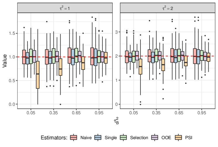
We simulated data from the linear model (2.1). We fixed βj2=τ𝐁25\beta_{j}^{2}=\frac{{\tau_{\bf{B}}^{2}}}{5} for j=1,…,5j=1,\dots,5, and βj2=τ2−τ𝐁2p−5\beta_{j}^{2}=\frac{{\tau^{2}-\tau_{\bf{B}}^{2}}}{{p-5}} for j=6,…,pj=6,\dots,p, where τ2\tau^{2} and τ𝐁2\tau_{\bf{B}}^{2} vary among different scenarios. The covariates were generated from the centered exponential distribution, i.e., Xi​j​∼i​i​d​Exp​(1)−1,X_{ij}\overset{iid}{\sim}\text{Exp}(1)-1, i=1,…,ni=1,\dots,n, j=1,…,pj=1,\dots,p. The noise ε\varepsilon was generated from the standard normal distribution. The number of observations and covariates is n=p=300n=p=300, and the residual variance σ2\sigma^{2} equals to 11. For each scenario, we generated 100 independent datasets and estimated τ2\tau^{2} by using the different estimators. Boxplots of the estimates are plotted in Figure 1 and results of the RMSE are given in Table 1. Since the ridge-based estimator of τ2\tau^{2} is highly biased, it is not comparable to the other proposed estimators and we omit it from the figures below. Code for reproducing the results is available at https://git.io/Jt6bC.

Table 1 shows the mean, the root mean square error (RMSE), and the relative improvement with respect to the naive τ^2\hat{\tau}^{2} for the different estimators. Standard errors are given in parenthesis. Important points to notice:

  • •

    Both of the proposed estimators Tc^∗T_{\hat{c}^{*}} and TγT_{\gamma} and the oracle estimator To​r​a​c​l​eT_{oracle} improve the naive estimator in all scenarios. When τ2=2,\tau^{2}=2, these improvements are more substantial than for the case of τ2=1\tau^{2}=1.

  • •

    The improved estimators are complementary to each other, i.e., for small values of τ𝐁2\tau^{2}_{\bf B} the Single estimator Tc^∗T_{\hat{c}^{*}} performs better than the Selection estimator TγT_{\gamma}, and the opposite occurs for large values of τ𝐁2.\tau^{2}_{\bf B}. For example, when τ2=1\tau^{2}=1 and τ𝐁2=5%,\tau^{2}_{\bf{B}}=5\%, the Single estimator Tc^∗T_{\hat{c}^{*}} improves the naive estimator by 26%26\% and when τ𝐁2=95%\tau^{2}_{\bf{B}}=95\%, the Selection estimator TγT_{\gamma} improves the naive by 23%23\%. This aligns with the result shown in Example 2.4.

  • •

    The PSI and ridge estimators perform poorly in a non-sparse setting. For example, when τ2=1\tau^{2}=1 and τ𝐁2=35%\tau^{2}_{\bf{B}}=35\% their RMSE are larger than the RMSE of the naive estimator by 47%47\% and 226%226\%, respectively. Notice that the RMSE of the ridge estimator is large also under the sparse setting.
Refer to caption
Figure 1: Boxplots representing the estimators’ distribution. The x-axis stands for τ𝐁2\tau^{2}_{\bf{B}}. The red dashed is the true value of τ2.\tau^{2}.

Figure 2 plots the RMSE of each estimator as a function of the sparsity level τ𝐁2\tau^{2}_{\bf B} and the signal level τ2.\tau^{2}. It is demonstrated that the Single and Selection estimators estimators improve (i.e., lower or equal RMSE) the naive estimator in all settings.

Refer to caption
Figure 2: Root mean square error (RMSE) for the different estimators. The x-axis stands for the sparsity level τ𝐁2\tau^{2}_{\bf B}.
Table 1: Summary statistics for the proposed estimators; n=p=300.n=p=300. Mean, root mean square error (RMSE) and percentage change from the naive estimator (in terms of RMSE) are shown. Simulation standard errors are shown in parenthesis. The table results were computed over 100100 simulated datasets for each setting. An estimate for the standard error of RMSE was calculated using the delta method. The estimator with the lowest RMSE (excluding the oracle) is in bold.
τ𝐁2\tau^{2}_{\bf{B}} τ2\tau^{2} Estimator Mean RMSE % Change
5% 1 naive 1.01 (0.051) 0.226 (0.035) 0
5% 1 OOE 1.01 (0.037) 0.165 (0.023) -26.99
5% 1 PSI 0.63 (0.08) 0.514 (0.064) 127.43
5% 1 Selection 1.01 (0.051) 0.225 (0.034) -0.44
5% 1 Single 0.97 (0.037) 0.168 (0.024) -25.66
5% 1 Ridge 0.21 (0.003) 0.789 (0.003) 213.1
35% 1 naive 1.02 (0.054) 0.242 (0.041) 0
35% 1 OOE 1.01 (0.039) 0.173 (0.027) -28.51
35% 1 PSI 0.77 (0.061) 0.356 (0.052) 47.11
35% 1 Selection 1.02 (0.052) 0.231 (0.035) -4.55
35% 1 Single 0.98 (0.044) 0.194 (0.033) -19.83
35% 1 Ridge 0.18 (0.003) 0.825 (0.003) 226.09
65% 1 naive 1.02 (0.057) 0.256 (0.046) 0
65% 1 OOE 1.01 (0.042) 0.185 (0.03) -27.73
65% 1 PSI 0.87 (0.047) 0.246 (0.036) -3.91
65% 1 Selection 1.02 (0.05) 0.224 (0.034) -12.5
65% 1 Single 1 (0.053) 0.235 (0.038) -8.2
65% 1 Ridge 0.13 (0.002) 0.868 (0.002) 213.36
95% 1 naive 1.02 (0.062) 0.278 (0.048) 0
95% 1 OOE 1.01 (0.045) 0.202 (0.033) -27.34
95% 1 PSI 0.98 (0.035) 0.157 (0.023) -43.53
95% 1 Selection 1.02 (0.048) 0.214 (0.034) -23.02
95% 1 Single 1.01 (0.063) 0.278 (0.047) 0
95% 1 Ridge 0.11 (0.001) 0.894 (0.001) 190.26
5% 2 naive 2.01 (0.039) 0.39 (0.027) 0
5% 2 OOE 2.01 (0.025) 0.245 (0.014) -37.18
5% 2 PSI 1.54 (0.052) 0.692 (0.052) 77.44
5% 2 Selection 2.01 (0.039) 0.386 (0.027) -1.03
5% 2 Single 1.94 (0.026) 0.264 (0.02) -32.31
5% 2 Ridge 0.33 (0.004) 1.672 (0.004) 282.61
35% 2 naive 2.02 (0.043) 0.427 (0.035) 0
35% 2 OOE 2.01 (0.025) 0.254 (0.017) -40.52
35% 2 PSI 1.66 (0.044) 0.554 (0.04) 29.74
35% 2 Selection 2.02 (0.04) 0.397 (0.027) -7.03
35% 2 Single 1.96 (0.033) 0.326 (0.023) -23.65
35% 2 Ridge 0.25 (0.004) 1.748 (0.004) 306.51
65% 2 naive 2.03 (0.046) 0.456 (0.04) 0
65% 2 OOE 2 (0.027) 0.272 (0.019) -40.35
65% 2 PSI 1.78 (0.034) 0.403 (0.028) -11.62
65% 2 Selection 2.03 (0.037) 0.372 (0.024) -18.42
65% 2 Single 1.99 (0.041) 0.411 (0.03) -9.87
65% 2 Ridge 0.18 (0.002) 1.819 (0.002) 287.02
95% 2 naive 2.04 (0.049) 0.494 (0.042) 0
95% 2 OOE 2 (0.03) 0.296 (0.022) -40.08
95% 2 PSI 1.96 (0.025) 0.255 (0.018) -48.38
95% 2 Selection 2.03 (0.033) 0.329 (0.024) -33.4
95% 2 Single 2.01 (0.05) 0.494 (0.041) 0
95% 2 Ridge 0.15 (0.002) 1.855 (0.002) 246.08

In the following we consider the case that the distribution of the covariates is only partially known. It is assumed that a large amount of unlabeled data is available and the distribution of the covariates is estimated based on this data. Specifically, we assume that additional sample of NN i.i.d observations Xn+1,…,Xn+NX_{n+1},...,X_{n+N} are given while the responses Yn+1,…,Yn+NY_{n+1},...,Y_{n+N} are not. Rather than treating μ≡E⁡(X)\mu\equiv E(X) and 𝚺≡Cov​(X){\bf\Sigma}\equiv\text{Cov}(X) as known, we estimate these parameters by their plug-in estimators, μ^≡1N​∑i=n+1n+NXi\hat{\mu}\equiv\frac{1}{N}\sum_{i={n+1}}^{n+N}X_{i} and 𝚺^≡1N​∑i=n+1n+N(Xi−𝟏​μ^)​(Xi−𝟏​μ^)T{\bf\hat{\Sigma}}\equiv\frac{1}{N}\sum_{i=n+1}^{n+N}(X_{i}-{\bf 1}\hat{\mu})(X_{i}-{\bf 1}\hat{\mu})^{T}, where 𝟏≡(1,…,1)T{\bf 1}\equiv~(1,\dots,1)^{T}. We then apply the linear transformation, X↦𝚺^−1/2(X−μ^),X\mapsto{\bf\hat{\Sigma}}^{-1/2}(X-\hat{\mu}), which corresponds the transformation shown in Section 2.2.1, and apply our estimators to the transformed XX. We repeated the simulation study above for different values of N.N.

Table 2 is similar to Table 1 but includes different values of NN rather than different values of τ𝐁2.\tau^{2}_{\bf B}. For simplicity we present only the scenario of τ2=1\tau^{2}=1 and τ𝐁2=0.35\tau^{2}_{\bf B}=0.35 but the results for other scenarios are similar. It can be observed from the table that for large values of NN the results are fairly similar to those in Table 1.

Table 2: Summary statistics similar to Table 1 ; n=p=300;n=p=300; τ𝐁2=0.65;\tau^{2}_{\bf B}=0.65; τ2=1.\tau^{2}=1.
NN Estimator Mean RMSE % Change
5000 naive 0.96 (0.025) 0.255 (0.021) 0
5000 OOE 0.98 (0.018) 0.179 (0.011) -29.8
5000 Selection 0.99 (0.025) 0.247 (0.018) -3.14
5000 Single 0.94 (0.023) 0.238 (0.021) -6.67
10000 naive 0.98 (0.024) 0.242 (0.017) 0
10000 OOE 0.98 (0.02) 0.2 (0.013) -17.36
10000 Selection 0.98 (0.022) 0.219 (0.013) -9.5
10000 Single 0.95 (0.023) 0.232 (0.016) -4.13
20000 naive 1.03 (0.027) 0.267 (0.015) 0
20000 OOE 1.03 (0.02) 0.201 (0.017) -24.72
20000 Selection 1.01 (0.023) 0.233 (0.016) -12.73
20000 Single 1.01 (0.026) 0.256 (0.015) -4.12

2.6 Generalization to Other Estimators

The suggested methodology in this paper is not limited to improving only the naive estimator, but can also be generalized to other estimators. The key is to add zero-estimators that are highly correlated with our initial estimator of τ2\tau^{2}; see Equation (2.3.1). Unlike the naive estimator, which is represented by a closed-form expression, other common estimators, such as the EigenPrism estimator (Janson et al. 2017), are computed numerically by solving a convex optimization problem. For a given zero-estimator, this makes the task of estimating the optimal-coefficient c∗c^{*} more challenging than before. To overcome this challenge, we approximate the optimal coefficient c∗c^{*} using bootstrap samples. We present a general algorithm that achieves improvement without claiming optimality. The algorithm is based on adding a single zero-estimator as in Section 2.4.2. A different version of the above algorithm, in which only a subset of covariates are used as for zero-estimators terms, was also used and is referred below to as the Selection estimator. See details in Remark 2.10 in the Appendix

Input: A dataset (𝐗,𝐘)\left({{\bf{X}},{\bf{Y}}}\right), an initial estimator τ~2\tilde{\tau}^{2}.
  1. 1.

    Calculate an initial estimator τ~2\tilde{\tau}^{2} of τ2\tau^{2}.

  2. 2.

    Bootstrap step:

    • •

      Resample with replacement nn observations from (𝐗,𝐘)\left({{{\bf{X}}},{{\bf{Y}}}}\right).

    • •

      Calculate the initial estimator τ~2\tilde{\tau}^{2} of τ2.\tau^{2}.

    • •

      Calculate the zero-estimator g¯n=1n​∑i=1ngi{\bar{g}_{n}}=\frac{1}{n}\sum\limits_{i=1}^{n}{{g_{i}}} where gi=∑j<j′Xi​j​Xi​j′{g_{i}}=\sum\limits_{j<j^{\prime}}{{X_{ij}}{X_{ij^{\prime}}}}.

    This procedure is repeated BB times in order to produce (τ~2)∗1,…,(τ~2)∗B(\tilde{\tau}^{2})^{*1},...,(\tilde{\tau}^{2})^{*B} and gn∗1,…,gn∗Bg_{n}^{*1},...,g_{n}^{*B}.

  3. 3.

    Approximate the coefficient c∗c^{*} by

    c~∗=Cov​(τ~2,g¯n)^Var​(g¯n),\tilde{c}^{*}=\frac{{\widehat{\text{Cov}\left({\tilde{\tau}^{2},{\bar{g}_{n}}}\right)}}}{{\text{Var}\left({{\bar{g}_{n}}}\right)}}\,,

    where Cov​(⋅)^\widehat{{\text{Cov}}\left(\cdot\right)} denotes the empirical covariance from the bootstrap samples, and Var​(g¯n)\text{Var}(\bar{g}_{n}) is known by the semi-supervised setting.

Result: Return the empirical estimator Te​m​p=τ~2−c~∗​g¯n{T_{emp}}={\tilde{\tau}^{2}}-{\tilde{c}^{*}}{\bar{g}_{n}}.
Algorithm 2 Empirical Estimators

We illustrate the improvement obtained by Algorithm 2 by choosing τ~2\tilde{\tau}^{2} to be the EigenPrism procedure (Janson et al. 2017), but other estimators can be used as well. We consider the same setting as in Section 2.5. The number of bootstrap samples is M=100.M=100. Results are given in Table 3 and the code for reproducing the results is available at https://git.io/Jt6bC.

The simulation results appear in Table 3 and in Figure 3. Both empirical estimators show an improvement over the EigenPrism estimator τ~2.\tilde{\tau}^{2}. The results here are fairly similar to the results shown for the naive estimator in Section 2.5, with just a smaller degree of improvement. As before, the Single and Selection estimators are complementary to each other, i.e., for small values of τ𝐁2\tau^{2}_{\bf B} the Single estimator performs better than the Selection estimator and the opposite occurs for large values of τ𝐁2\tau^{2}_{\bf B} This highlights the fact that the zero-estimator approach is not limited to improving only the naive estimator but rather has the potential to improve other estimators as well.

Table 3: Summary statistics similar to Table 1.
τ𝐁2\tau^{2}_{\bf{B}} τ2\tau^{2} Estimator Mean RMSE % Change
5% 1 Eigenprism 0.98 (0.019) 0.195 (0.012) 0
5% 1 Single 0.98 (0.018) 0.183 (0.012) -6.15
5% 1 Selection 0.98 (0.02) 0.195 (0.013) 0
35% 1 Eigenprism 0.99 (0.02) 0.198 (0.013) 0
35% 1 Single 0.99 (0.019) 0.193 (0.013) -2.53
35% 1 Selection 0.99 (0.02) 0.197 (0.013) -0.51
65% 1 Eigenprism 1 (0.021) 0.206 (0.013) 0
65% 1 Single 1 (0.021) 0.205 (0.013) -0.49
65% 1 Selection 1 (0.02) 0.199 (0.013) -3.4
95% 1 Eigenprism 1.01 (0.022) 0.215 (0.014) 0
95% 1 Single 1.01 (0.022) 0.215 (0.014) 0
95% 1 Selection 1.01 (0.02) 0.201 (0.013) -6.51
5% 2 EigenPrism 2.05 (0.029) 0.292 (0.018) 0
5% 2 Single 2.03 (0.026) 0.262 (0.016) -10.27
5% 2 Selection 2.05 (0.029) 0.292 (0.017) 0
35% 2 EigenPrism 2.02 (0.029) 0.287 (0.02) 0
35% 2 Single 2.01 (0.027) 0.272 (0.02) -5.23
35% 2 Selection 2.01 (0.028) 0.281 (0.02) -2.09
65% 2 EigenPrism 2.01 (0.03) 0.296 (0.023) 0
65% 2 Single 2 (0.029) 0.292 (0.023) -1.35
65% 2 Selection 1.99 (0.028) 0.28 (0.021) -5.41
95% 2 EigenPrism 1.99 (0.031) 0.31 (0.025) 0
95% 2 Single 1.99 (0.031) 0.31 (0.025) 0
95% 2 Selection 1.97 (0.028) 0.279 (0.021) -10
Refer to caption
Figure 3: Root mean square error (RMSE) for the proposed estimators. The x-axis stands for the sparsity level τ𝐁2\tau^{2}_{\bf B}.

2.7 Discussion and Future Work

This paper presents a new approach for improving estimation of the explained variance τ2\tau^{2} of a high-dimensional regression model in a semi-supervised setting without assuming sparsity. The key idea is to use a zero-estimator that is correlated with the initial unbiased estimator of τ2\tau^{2} in order to lower its variance without introducing additional bias. The semi-supervised setting, where the number of observations is much greater than the number of responses, allows us to construct such zero-estimators. We introduced a new notion of optimality with respect to zero-estimators and presented an oracle-estimator that achieves this type of optimality. We proposed two different (non-oracle) estimators that showed a significant reduction, but not optimal, in the asymptotic variance of the naive estimator. Our simulations showed that our approach can be generalized to other types of initial estimators other than the naive estimator.

Many open questions remain for future research. While our proposed estimators improved the naive estimator, it did not achieve the optimal improvement of the oracle estimator. Thus, it remains unclear if and how one can achieve optimal improvement. Moreover, the theory developed in this work relies on a strong assumption about unsupervised data size, i.e., N=∞N=\infty. Thus, generalizing our suggested theory by relaxing this assumption to allow for a general setting with a finite N≫nN\gg n is a natural direction for future work. A more ambitious future goal would be to extend the suggested approach to generalized linear models (GLM), and specifically to logistic regression. In this case, the concepts of signal and noise levels are less clear and are more challenging to define.

Supplementary Material

Proof of Lemma 2.1:
Notice that XT​𝐘=(∑i=1nWi​1,…,∑i=1nWi​p)T{{\textbf{X}}^{T}}{\bf{Y}}={\left({\sum\limits_{i=1}^{n}{{W_{i1}}},...,\sum\limits_{i=1}^{n}{{W_{ip}}}}\right)^{T}} where X is the n×pn\times p design matrix and Y=(Y1,…,Yn)T\textbf{Y}=(Y_{1},...,Y_{n})^{T}. Thus, the naive estimator can be also written as

τ^2=1n⁡(n−1)​∑i1≠i2∑j=1pWi1​j​Wi2​j=‖XT​𝐘‖2−∑j=1p∑i=1nWi​j2n⁡(n−1).\hat{\tau}^{2}=\frac{1}{{n\left({n-1}\right)}}\sum\limits_{{i_{1}}\neq{i_{2}}}{\sum\limits_{j=1}^{p}{W_{{i_{1}}j}{W_{{i_{2}}j}}=}}\frac{{{{\left\|{{{\textbf{X}}^{T}}{\bf{Y}}}\right\|}^{2}}-\sum\limits_{j=1}^{p}{\sum\limits_{i=1}^{n}{W_{ij}^{2}}}}}{{n\left({n-1}\right)}}.

The Dicker estimate for τ2\tau^{2} ia given by τ^D​i​c​k​e​r2≡‖XT​𝐘‖2−p​‖𝐘‖2n⁡(n+1).\hat{\tau}^{2}_{Dicker}\equiv\frac{{{{\left\|{{{\textbf{X}}^{T}}{\bf{Y}}}\right\|}^{2}}-p{{\left\|{\bf{Y}}\right\|}^{2}}}}{{n\left({n+1}\right)}}. We need to prove that root-nn times the difference between the estimators converges in probability to zero, i.e., n​(τ^D​i​c​k​e​r2−τ^2)​→𝑝​0\sqrt{n}\left(\hat{\tau}^{2}_{Dicker}-\hat{\tau}^{2}\right)\overset{p}{\rightarrow}0. We have,

n​(τ^D​i​c​k​e​r2−τ^2)=n​(‖𝐗T​𝐘‖2−p​‖𝐘‖2n⁡(n+1)−‖𝐗T​𝐘‖2−∑j=1p∑i=1nWi​j2n⁡(n−1))=n​(∑j=1p∑i=1nWi​j2n⁡(n−1)−p​‖𝐘‖2n⁡(n+1)−2​‖𝐗T​𝐘‖2n​(n−1)​(n+1)).\begin{split}\sqrt{n}\left(\hat{\tau}^{2}_{Dicker}-\hat{\tau}^{2}\right)&=\sqrt{n}\left({\frac{{{{\left\|{{{\bf{X}}^{T}}{\bf{Y}}}\right\|}^{2}}-p{{\left\|{\bf{Y}}\right\|}^{2}}}}{{n\left({n+1}\right)}}-\frac{{{{\left\|{{{\bf{X}}^{T}}{\bf{Y}}}\right\|}^{2}}-\sum\limits_{j=1}^{p}{\sum\limits_{i=1}^{n}{W_{ij}^{2}}}}}{{n\left({n-1}\right)}}}\right)\\ &=\sqrt{n}\left({\frac{{\sum\limits_{j=1}^{p}{\sum\limits_{i=1}^{n}{W_{ij}^{2}}}}}{{n\left({n-1}\right)}}-\frac{{p{{\left\|{\bf{Y}}\right\|}^{2}}}}{{n\left({n+1}\right)}}-\frac{{2{{\left\|{{{\bf{X}}^{T}}{\bf{Y}}}\right\|}^{2}}}}{{n\left({n-1}\right)\left({n+1}\right)}}}\right).\end{split} (2.23)

It is enough to prove that:

  1. 1.

    n−1.5​(∑j=1p∑i=1nWi​j2−p​‖𝐘‖2)​→𝑝​0,n^{-1.5}\left(\sum\limits_{j=1}^{p}\sum\limits_{i=1}^{n}{W_{ij}^{2}}-p{{\left\|{\bf{Y}}\right\|}^{2}}\right)\overset{p}{\rightarrow}0,

  2. 2.

    n−2.5​(‖𝐗T​𝐘‖2)​→𝑝​0.n^{-2.5}\left({{{{\left\|{{{\bf{X}}^{T}}{\bf{Y}}}\right\|}^{2}}}}\right)\overset{p}{\rightarrow}0.

We start with the first term,

n−1.5​(∑j=1p∑i=1nWi​j2−p​‖𝐘‖2)=n−1.5​(∑j=1p∑i=1nYi2​Xi​j2−p​∑i=1nYi2)=n−1.5​(∑i=1nYi2​∑j=1pXi​j2−p​∑i=1nYi2)=n−0.5​∑i=1nYi2​[1n​∑j=1p(Xi​j2−1)]≡n−0.5​∑i=1nωin^{-1.5}\left(\sum\limits_{j=1}^{p}\sum\limits_{i=1}^{n}{W_{ij}^{2}}-p{{\left\|{\bf{Y}}\right\|}^{2}}\right)=n^{-1.5}\left({\sum\limits_{j=1}^{p}{\sum\limits_{i=1}^{n}{Y_{i}^{2}X_{ij}^{2}}}-p\sum\limits_{i=1}^{n}{Y_{i}^{2}}}\right)\\ =n^{-1.5}\left({\sum\limits_{i=1}^{n}{Y_{i}^{2}\sum\limits_{j=1}^{p}{X_{ij}^{2}}}-p\sum\limits_{i=1}^{n}{Y_{i}^{2}}}\right)=n^{-0.5}\sum\limits_{i=1}^{n}{Y_{i}^{2}}\left[{\frac{1}{n}\sum\limits_{j=1}^{p}{\left({X_{ij}^{2}-1}\right)}}\right]\equiv n^{-0.5}\sum\limits_{i=1}^{n}{{\omega_{i}}} (2.24)

where ωi=Yi2​[1n​∑j{Xi​j2−1}].{\omega_{i}}=Y_{i}^{2}\left[{\frac{1}{n}\sum\limits_{j}{\left\{{X_{ij}^{2}-1}\right\}}}\right]. Notice that ωi\omega_{i} depends on nn but this is suppressed in the notation. In order to show that n−0.5​∑i=1nωi​→𝑝​0,n^{-0.5}\sum\limits_{i=1}^{n}{{\omega_{i}}}\overset{p}{\rightarrow}0, it is enough to show that E⁡(n−0.5​∑i=1nωi)→0E\left({n^{-0.5}\sum\limits_{i=1}^{n}{{\omega_{i}}}}\right)\to 0 and Var​(n−0.5​∑i=1nωi)→0.\text{Var}\left({n^{-0.5}\sum\limits_{i=1}^{n}{{\omega_{i}}}}\right)\to 0. Moreover, since E⁡(n−0.5​∑i=1nωi)=n​E​(ωi)E\left({n^{-0.5}\sum\limits_{i=1}^{n}{{\omega_{i}}}}\right)=\sqrt{n}E\left({{\omega_{i}}}\right) and Var​(n−0.5​∑i=1nωi)=Var​(ωi)=E⁡(ωi2)−[E⁡(ωi)]2,\text{Var}\left({n^{-0.5}\sum\limits_{i=1}^{n}{{\omega_{i}}}}\right)=\text{Var}\left({{\omega_{i}}}\right)=E\left({\omega_{i}^{2}}\right)-{\left[{E\left({{\omega_{i}}}\right)}\right]^{2}}, it is enough to show that n​E​(ωi)\sqrt{n}E\left({{\omega_{i}}}\right) and E⁡(ωi2)E\left({\omega_{i}^{2}}\right) converge to zero.
Consider now n​E​(ωi)\sqrt{n}E\left({{\omega_{i}}}\right). By (2.24) we have

∑i=1nωi=1n​[∑j=1p∑i=1nWi​j2−p​‖𝐘‖2].\sum\limits_{i=1}^{n}{{\omega_{i}}}=\frac{1}{n}\left[{\sum\limits_{j=1}^{p}{\sum\limits_{i=1}^{n}{W_{ij}^{2}}}-p{{\left\|{\bf{Y}}\right\|}^{2}}}\right].

Taking expectation of both sides,

∑i=1nE⁡(ωi)=1n​[∑j=1p∑i=1nE⁡(Wi​j2)−p​E​(‖𝐘‖2)].\sum\limits_{i=1}^{n}{E\left({{\omega_{i}}}\right)}=\frac{1}{n}\left[{\sum\limits_{j=1}^{p}{\sum\limits_{i=1}^{n}{E\left({W_{ij}^{2}}\right)}}-pE\left({{{\left\|{\bf{Y}}\right\|}^{2}}}\right)}\right].

Now, notice that

E⁡(Wi​j2)=E⁡[Xi​j2​(βT​X+ε)2]=‖β‖2+σ2+βj2​[E⁡(Xi​j4)−1]=τ2+σ2+2​βj2.E(W_{ij}^{2})=E[X_{ij}^{2}(\beta^{T}X+\varepsilon)^{2}]={\left\|\beta\right\|^{2}}+{\sigma^{2}}+\beta_{j}^{2}[E(X_{ij}^{4})-1]={\tau^{2}}+{\sigma^{2}}+2\beta_{j}^{2}. (2.25)

Also notice that Yi2/(σε2+τ2)∼χ12,Y_{i}^{2}/\left({\sigma_{\varepsilon}^{2}+{\tau^{2}}}\right)\sim\chi_{1}^{2}, and hence E⁡(‖𝐘‖2)=n⁡(τ2+σ2)E\left({{{\left\|{\bf{Y}}\right\|}^{2}}}\right)=n\left({{\tau^{2}}+{\sigma^{2}}}\right). Therefore,

n​E​(ωi)\displaystyle nE\left({{\omega_{i}}}\right) =1n​[∑j=1p∑i=1n(τ2+σ2+2​βj2)−p​n​(τ2+σ2)]\displaystyle=\frac{1}{n}\left[{\sum\limits_{j=1}^{p}{\sum\limits_{i=1}^{n}{\left({{\tau^{2}}+{\sigma^{2}}+2\beta_{j}^{2}}\right)}}-pn\left({{\tau^{2}}+{\sigma^{2}}}\right)}\right]
=1n​[∑i=1n[p⁡(τ2+σ2)+2​τ2]−p​n​(τ2+σ2)]=2​τ2\displaystyle=\frac{1}{n}\left[{\sum\limits_{i=1}^{n}{\left[{p\left({{\tau^{2}}+{\sigma^{2}}}\right)+2{\tau^{2}}}\right]-pn\left({{\tau^{2}}+{\sigma^{2}}}\right)}}\right]=2{\tau^{2}}

which implies that n​E​(ωi)=2​τ2n​→​0.\sqrt{n}E\left({{\omega_{i}}}\right)=\frac{{2{\tau^{2}}}}{{\sqrt{n}}}\overset{}{\rightarrow}~0.

Consider now E⁡(ωi2)E(\omega_{i}^{2}). By Cauchy-Schwartz,

E⁡(ωi2)=E⁡(Yi4​[n−1​∑j=1p{Xi​j2−1}]2)≤{E⁡(Yi8)}1/2​{E⁡([n−1​∑j=1p{Xi​j2−1}]4)}1/2.E\left({\omega_{i}^{2}}\right)=E\left({Y_{i}^{4}{{\left[{n^{-1}\sum\limits_{j=1}^{p}{\left\{{X_{ij}^{2}-1}\right\}}}\right]}^{2}}}\right)\leq{\left\{{E\left({Y_{i}^{8}}\right)}\right\}^{1/2}}{\left\{{E\left({{{\left[{n^{-1}\sum\limits_{j=1}^{p}{\left\{{X_{ij}^{2}-1}\right\}}}\right]}^{4}}}\right)}\right\}^{1/2}}.

Notice that Yi∼N⁡(0,τ2+σ2){Y_{i}}\sim N\left({0,{\tau^{2}}+{\sigma^{2}}}\right) by construction and therefore E⁡(Yi8)=O⁡(1)E(Y_{i}^{8})=O(1) as nn and pp go to infinity. Let Vj=Xi​j2−1V_{j}=X_{ij}^{2}-1 and notice that E⁡(Vj)=0.E(V_{j})=0. We have

E⁡([n−1​∑j=1p{Xi​j2−1}]4)=E⁡([n−1​∑j=1pVj]4)=n−4​∑j1,j2,j3,j4E⁡(Vj1​Vj2​Vj3​Vj4).E\left({{{\left[{{n^{-1}}\sum\limits_{j=1}^{p}{\left\{{X_{ij}^{2}-1}\right\}}}\right]}^{4}}}\right)=E\left({{{\left[{{n^{-1}}\sum\limits_{j=1}^{p}{{V_{j}}}}\right]}^{4}}}\right)={n^{-4}}\sum\limits_{{j_{1}},{j_{2}},{j_{3}},{j_{4}}}{E\left({{V_{{j_{1}}}}{V_{{j_{2}}}}{V_{{j_{3}}}}{V_{{j_{4}}}}}\right)}.

The expectation ∑j1,j2,j3,j4E⁡(Vj1​Vj2​Vj3​Vj4)\sum\limits_{{j_{1}},{j_{2}},{j_{3}},{j_{4}}}{E\left({{V_{{j_{1}}}}{V_{{j_{2}}}}{V_{{j_{3}}}}{V_{{j_{4}}}}}\right)} is not 0 when j1=j2j_{1}=j_{2} and j3=j4j_{3}=j_{4} (up to permutations) or when all terms are equal. In the first case we have

∑j≠j′E⁡(Vj2​Vj′2)=∑j≠j′[E⁡(Vj2)]2=p⁡(p−1)​[E⁡{(Xi​j2−1)2}]2≤C1​p2,\sum\limits_{j\neq j^{\prime}}{E\left({V_{j}^{2}V_{j^{\prime}}^{2}}\right)=}\sum\limits_{j\neq j^{\prime}}{{{\left[{E\left({V_{j}^{2}}\right)}\right]}^{2}}=}p\left({p-1}\right){\left[{E\left\{{{{\left({X_{ij}^{2}-1}\right)}^{2}}}\right\}}\right]^{2}}\leq C_{1}p^{2},

for a positive constant C1.C_{1}. In the second case we have ∑j=1pE⁡(Vj4)=p​E​[(Xi​j2−1)4]≤C2​p,\sum\limits_{j=1}^{p}{E\left({V_{j}^{4}}\right)=}pE\left[{{{\left({X_{ij}^{2}-1}\right)}^{4}}}\right]\leq C_{2}p, for a positive constant C2C_{2}. Hence, as pp and nn have the same order of magnitude, we have

{E⁡[(n−1​∑j=1p{Xi​j2−1})4]}1/2\displaystyle{\left\{{E\left[{{{\left({{n^{-1}}\sum\limits_{j=1}^{p}{\left\{{X_{ij}^{2}-1}\right\}}}\right)}^{4}}}\right]}\right\}^{1/2}} ={n−4​∑j1,j2,j3,j4E⁡(Vj1​Vj2​Vj3​Vj4)}1/2\displaystyle={\left\{{{n^{-4}}\sum\limits_{{j_{1}},{j_{2}},{j_{3}},{j_{4}}}{E\left({{V_{{j_{1}}}}{V_{{j_{2}}}}{V_{{j_{3}}}}{V_{{j_{4}}}}}\right)}}\right\}^{1/2}}
≤{n−4⋅O⁡(p2)}1/2≤K/n,\displaystyle\leq{\left\{{{n^{-4}}\cdot O\left({{p^{2}}}\right)}\right\}^{1/2}}\leq K/n,

which implies E⁡(ωi2)≤K1/n→0,E(\omega_{i}^{2})\leq K_{1}/n\rightarrow 0, where KK and K1K_{1} are positive constants. This completes the proof that

n−1.5​(∑j=1p∑i=1nWi​j2−p​‖𝐘‖2)​→𝑝​0.n^{-1.5}\left(\sum\limits_{j=1}^{p}\sum\limits_{i=1}^{n}{W_{ij}^{2}}-p{{\left\|{\bf{Y}}\right\|}^{2}}\right)\overset{p}{\rightarrow}~0.

We now move to prove that n−2.5​(‖𝐗T​𝐘‖2)​→𝑝​0.n^{-2.5}\left({{{{\left\|{{{\bf{X}}^{T}}{\bf{Y}}}\right\|}^{2}}}}\right)\overset{p}{\rightarrow}0. By Markov’s inequality, for ε>0\varepsilon>0

P⁡(n−2.5​‖𝐗T​𝐘‖2>ε)≤n−2.5​E​(‖𝐗T​𝐘‖2)/ε.P\left({{n^{-2.5}}{{\left\|{{{\bf{X}}^{T}}{\bf{Y}}}\right\|}^{2}}>\varepsilon}\right)\leq{n^{-2.5}}E\left({{{\left\|{{{\bf{X}}^{T}}{\bf{Y}}}\right\|}^{2}}}\right)/\varepsilon.

Thus, it is enough to show that n−2​E​(‖𝐗T​𝐘‖2){n^{-2}}E\left({{{\left\|{{{\bf{X}}^{T}}{\bf{Y}}}\right\|}^{2}}}\right) is bounded. Notice that

E⁡(‖𝐗T​𝐘‖2)=∑i1,i2∑j=1pE⁡(Wi1​j​Wi2​j)=∑i=1n∑j=1pE⁡(Wi​j2)+∑i1≠i2∑j=1pE⁡(Wi1​j​Wi2​j)=∑i=1n∑j=1p(τ2+σ2+2​βj2)+∑i1≠i2∑j=1pβj2=n⁡[p⁡(τ2+σ2)+2​τ2]+n⁡(n−1)​τ2=n⁡[p⁡(τ2+σ2)+(n+1)​τ2],\begin{split}E\left({{{\left\|{{{\bf{X}}^{T}}{\bf{Y}}}\right\|}^{2}}}\right)&=\sum\limits_{{i_{1}},{i_{2}}}{\sum\limits_{j=1}^{p}{E\left({{W_{{i_{1}}j}}{W_{{i_{2}}j}}}\right)}}=\sum\limits_{i=1}^{n}{\sum\limits_{j=1}^{p}{E\left({W_{ij}^{2}}\right)}}+\sum\limits_{{i_{1}}\neq{i_{2}}}{\sum\limits_{j=1}^{p}{E\left({{W_{{i_{1}}j}}{W_{{i_{2}}j}}}\right)}}\\ &=\sum\limits_{i=1}^{n}{\sum\limits_{j=1}^{p}{\left({{\tau^{2}}+{\sigma^{2}}+2\beta_{j}^{2}}\right)}}+\sum\limits_{{i_{1}}\neq{i_{2}}}{\sum\limits_{j=1}^{p}{\beta_{j}^{2}}}=n\left[{p\left({{\tau^{2}}+{\sigma^{2}}}\right)+2{\tau^{2}}}\right]+n\left({n-1}\right){\tau^{2}}\\ &=n\left[{p\left({{\tau^{2}}+{\sigma^{2}}}\right)+\left({n+1}\right){\tau^{2}}}\right],\end{split}

where we used (2.25) in the third equality. Therefore,

n−2​E​(‖𝐗T​𝐘‖2)=n−1​[p⁡(τ2+σ2)+(n+1)​τ2].{n^{-2}}E\left({{{\left\|{{{\bf{X}}^{T}}{\bf{Y}}}\right\|}^{2}}}\right)={n^{-1}}\left[{p\left({{\tau^{2}}+{\sigma^{2}}}\right)+\left({n+1}\right){\tau^{2}}}\right].

Since pp and nn have the same order of magnitude and τ2\tau^{2}+σ2\sigma^{2} is bounded by assumption, then n−2​E​(‖𝐗T​𝐘‖2){n^{-2}}E\left({{{\left\|{{{\bf{X}}^{T}}{\bf{Y}}}\right\|}^{2}}}\right) is also bounded. This completes the proof of n−2.5​(‖𝐗T​𝐘‖2)​→𝑝​0n^{-2.5}\left({{{{\left\|{{{\bf{X}}^{T}}{\bf{Y}}}\right\|}^{2}}}}\right)\overset{p}{\rightarrow}~0 and hence n​(τ^D​i​c​k​e​r2−τ^2)​→𝑝​0.\sqrt{n}\left({\hat{\tau}_{Dicker}^{2}-{{\hat{\tau}}^{2}}}\right)\overset{p}{\rightarrow}~0. ∎

Proof of Corollary 2.1:
According to Corollary 1 in Dicker 2014, we have

n​(τ^D​i​c​k​e​r−τ2)ψ​→𝐷​N​(0,1),\frac{{\sqrt{n}\left({{\hat{\tau}_{Dicker}}-{\tau^{2}}}\right)}}{\psi}\overset{D}{\rightarrow}N\left({0,1}\right),

where ψ=2​{(1+pn)​(σ2+τ2)2−σ4+3​τ4},\psi=2\left\{{\left({1+\frac{p}{n}}\right){{\left({\sigma^{2}+{\tau^{2}}}\right)}^{2}}-\sigma^{4}+3{\tau^{4}}}\right\}, given that p/np/n converges to a constant. Therefore we can write

n​(τ^2−τ2)ψ=1ψ​[n​(τ^2−τ^D​i​c​k​e​r)+n​(τ^D​i​c​k​e​r−τ2)],\frac{{\sqrt{n}\left({{{\hat{\tau}}^{2}}-{\tau^{2}}}\right)}}{\psi}=\frac{1}{\psi}\left[{\sqrt{n}\left({{{\hat{\tau}}^{2}}-{{\hat{\tau}}_{Dicker}}}\right)+\sqrt{n}\left({{{\hat{\tau}}_{Dicker}}-{\tau^{2}}}\right)}\right],

and obtain n​(τ^2−τ2ψ)​→𝐷​N​(0,1)\sqrt{n}\left({\frac{{{{\hat{\tau}}^{2}}-{\tau^{2}}}}{\psi}}\right)\overset{D}{\rightarrow}N(0,1)\, by Slutsky’s theorem. ∎

Proof of Proposition 2.1:
Let 𝐖i=(Wi​1,…,Wi​p)T{{\bf{W}}_{i}}={\left({{W_{i1}},...,{W_{ip}}}\right)^{T}} and notice that τ^2=1n⁡(n−1)​∑i1≠i2n∑j=1pWi1​j​Wi2​j\hat{\tau}^{2}=\frac{1}{{n\left({n-1}\right)}}\sum\limits_{{i_{1}}\neq{i_{2}}}^{n}\sum\limits_{j=1}^{p}{{W_{{i_{1}}j}}{W_{{i_{2}}j}}} is a U-statistic of order 2 with the kernel h⁡(𝐰1,𝐰2)=𝐰1T​𝐰2=∑j=1pw1​j​w2​jh\left({{{\bf{w}}_{1}},{{\bf{w}}_{2}}}\right)={\bf{w}}_{1}^{T}{{\bf{w}}_{2}}=\sum\limits_{j=1}^{p}{{w_{1j}}{w_{2j}}}, where 𝐰i∈ℝp{{\bf{w}}_{i}}\in{\mathbb{R}^{p}}.

By Theorem 12.3 in van der Vaart 2000,

Var​(τ^2)=4​(n−2)n⁡(n−1)​ζ1+2n⁡(n−1)​ζ2,{\text{Var}}\left({{{\hat{\tau}}^{2}}}\right)=\frac{{4\left({n-2}\right)}}{{n\left({n-1}\right)}}{\zeta_{1}}+\frac{2}{{n\left({n-1}\right)}}{\zeta_{2}}, (2.26)

where ζ1=Cov​[h⁡(𝐖1,𝐖2),h⁡(𝐖1,𝐖~2)]{\zeta_{1}}={\text{Cov}}\left[{h\left({{{\bf{W}}_{1}},{{\bf{W}}_{2}}}\right),h\left({{{\bf{W}}_{1}},{{\widetilde{\bf{{W}}}_{2}}}}\right)}\right] and ζ2=Cov​[h⁡(𝐖1,𝐖2),h⁡(𝐖1,𝐖2)]{\zeta_{2}}={\text{Cov}}\left[{h\left({{{\bf{W}}_{1}},{{\bf{W}}_{2}}}\right),h\left({{{\bf{W}}_{1}},{{\bf{W}}_{2}}}\right)}\right] where 𝐖~2\widetilde{\bf{{W}}}_{2} is an independent copy of 𝐖𝟐\bf{W}_{2}. Now, let 𝐀=E⁡(𝐖i​𝐖iT){\bf{A}}=E\left({{{\bf{W}}_{i}}{\bf{W}}_{i}^{T}}\right) be a p×pp\times p matrix and notice that

ζ1\displaystyle{\zeta_{1}} =Cov​[h⁡(𝐖1,𝐖2),h⁡(𝐖1,𝐖~2)]\displaystyle=\text{Cov}\left[{h\left({{{\bf{W}}_{1}},{{\bf{W}}_{2}}}\right),h\left({{{\bf{W}}_{1}},{{\widetilde{\bf{W}}}_{2}}}\right)}\right]
=∑j,j′pCov​(W1​j​W2​j,W1​j′​W~2​j′)=∑j,j′p(βj​βj′​E​[W1​j​W1​j′]−βj2​βj′2)\displaystyle=\sum\limits_{j,j^{\prime}}^{p}{\text{Cov}\left({{W_{1j}}{W_{2j}},{W_{1j^{\prime}}}{{\widetilde{W}}_{2j^{\prime}}}}\right)}=\sum\limits_{j,j^{\prime}}^{p}{\left({{\beta_{j}}{\beta_{j^{\prime}}}E\left[{{W_{1j}}{W_{1j^{\prime}}}}\right]-\beta_{j}^{2}\beta_{j^{\prime}}^{2}}\right)}
=βT​𝐀​β−‖β‖4\displaystyle={\beta^{T}}{\bf{A}}\beta-{\left\|\beta\right\|^{4}}

and

ζ2\displaystyle{\zeta_{2}} =Cov​[h⁡(𝐖1,𝐖2),h⁡(𝐖1,𝐖2)]\displaystyle={\text{Cov}}\left[{h\left({{{\bf{W}}_{1}},{{\bf{W}}_{2}}}\right),h\left({{{\bf{W}}_{1}},{{\bf{W}}_{2}}}\right)}\right]
=∑j,j′Cov​(W1​j​W2​j,W1​j′​W2​j′)=∑j,j′((E⁡[W1​j​W1​j′])2−βj2​βj′2)\displaystyle=\sum\limits_{j,j^{\prime}}{{\text{Cov}}\left({{W_{1j}}{W_{2j}},{W_{1j^{\prime}}}{W_{2j^{\prime}}}}\right)}=\sum\limits_{j,j^{\prime}}\left({{{\left({E\left[{{W_{1j}}{W_{1j^{\prime}}}}\right]}\right)}^{2}}-\beta_{j}^{2}\beta_{j^{\prime}}^{2}}\right)
=‖𝐀‖F2−‖β‖4,\displaystyle=\left\|{\bf{A}}\right\|_{F}^{2}-{\left\|\beta\right\|^{4}},

where ‖A‖F2\|\textbf{A}\|_{F}^{2} is the Frobenius norm of A.\textbf{A}. Thus, by rewriting (2.26) the variance of the naive estimator is given by

Var​(τ^2)=4​(n−2)n⁡(n−1)​[βT​𝐀​β−‖β‖4]+2n⁡(n−1)​[‖𝐀‖F2−‖β‖4].{\text{Var}}\left({{{\hat{\tau}}^{2}}}\right)=\frac{{4\left({n-2}\right)}}{{n\left({n-1}\right)}}\left[{{\beta^{T}}{\bf{A}}\beta-{{\left\|\beta\right\|}^{4}}}\right]+\frac{2}{{n\left({n-1}\right)}}\left[{\left\|{\bf{A}}\right\|_{F}^{2}-{{\left\|\beta\right\|}^{4}}}\right]. (2.27)

Proof of Proposition 2.2:
Notice that τ^2\hat{\tau}^{2} is consistent if Var​[τ^2]→n→∞0\text{Var}[\hat{\tau}^{2}]\xrightarrow{n\rightarrow\infty}0 since τ^2\hat{\tau}^{2} is unbiased. Thus, by (2.27) it is enough to require that βT​A​βn→n→∞0\frac{\beta^{T}\textbf{A}\beta}{n}\xrightarrow{n\rightarrow\infty}0 and ‖A‖F2n2→n→∞0\frac{\|\textbf{A}\|^{2}_{F}}{n^{2}}\xrightarrow{n\rightarrow\infty}0. The latter is assumed and we now show that the former also holds true. Let λ1≥…≥λp\lambda_{1}\geq...\geq\lambda_{p} be the eigenvalues of A and notice that A is symmetric. We have that n−2​λ12≤n−2​∑j=1pλj2=n−2​t​r​(A2)=n−2​‖A‖F2n^{-2}\lambda_{1}^{2}\leq n^{-2}\sum_{j=1}^{p}\lambda_{j}^{2}=n^{-2}tr(\textbf{A}^{2})=n^{-2}\|\textbf{A}\|_{F}^{2} and therefore (iii) implies that λ1n→n→∞0\frac{\lambda_{1}}{n}\xrightarrow{n\rightarrow\infty}0. Now, 1n​βT​A​β≡1n​‖β‖2​[(β‖β‖)T​A​β‖β‖]≤1n​‖β‖2​λ1→n→∞0,\frac{1}{n}\beta^{T}\textbf{A}\beta\equiv\frac{1}{n}\|\beta\|^{2}[(\frac{\beta}{\|\beta\|})^{T}\textbf{A}\frac{\beta}{\|\beta\|}]\leq\frac{1}{n}\|\beta\|^{2}\lambda_{1}\xrightarrow{n\rightarrow\infty}0, where the last limit follows from the assumption that τ2=O⁡(1),\tau^{2}=O(1), and from the fact that λ1n→n→∞0\frac{\lambda_{1}}{n}\xrightarrow{n\rightarrow\infty}0 . We conclude that Var​[τ^2]→n→∞0\text{Var}[\hat{\tau}^{2}]\xrightarrow{n\rightarrow\infty}0.

We now prove the moreover part, that is, independence of the columns of X implies that ‖A‖F2n2→n→∞0\frac{\|\textbf{A}\|^{2}_{F}}{n^{2}}\xrightarrow{n\rightarrow\infty}0. By definition we have ‖A‖F2=∑j,j′[E⁡(Wi​j​Wi​j′)]2.\|\textbf{A}\|_{F}^{2}=\sum_{j,j^{\prime}}[E(W_{ij}W_{ij^{\prime}})]^{2}. Notice that when j=j′j=j^{\prime} we have,

E⁡(Wi​j2)\displaystyle E\left({W_{ij}^{2}}\right) =E⁡(Xi​j2​Yi2)=E⁡(Xi​j2​[βT​Xi+εi]2)\displaystyle=E\left({X_{ij}^{2}Y_{i}^{2}}\right)=E\left({X_{ij}^{2}{{\left[{{\beta^{T}}{X_{i}}+{\varepsilon_{i}}}\right]}^{2}}}\right)
=E⁡(Xi​j2​[∑k,k′βk​βk′​Xi​k​Xi​k′+2​βT​Xi​εi+εi2])\displaystyle=E\left({X_{ij}^{2}\left[{\sum\limits_{k,k^{\prime}}{{\beta_{k}}{\beta_{k^{\prime}}}{X_{ik}}{X_{ik^{\prime}}}}+2{\beta^{T}}{X_{i}}{\varepsilon_{i}}+\varepsilon_{i}^{2}}\right]}\right)
=E⁡(Xi​j2​∑k,k′βk​βk′​Xi​k​Xi​k′)+0+E⁡(Xi​j2​εi2)\displaystyle=E\left({X_{ij}^{2}\sum\limits_{k,k^{\prime}}{{\beta_{k}}{\beta_{k^{\prime}}}{X_{ik}}{X_{ik^{\prime}}}}}\right)+0+E\left({X_{ij}^{2}\varepsilon_{i}^{2}}\right)
=E⁡(Xi​j2​∑k=1pβk2​Xi​k2)+E⁡(Xi​j2​∑k≠k′βk​βk′​Xi​k​Xi​k′)⏟0+σ2​E​(Xi​j2)\displaystyle=E\left({X_{ij}^{2}\sum\limits_{k=1}^{p}{\beta_{k}^{2}X_{ik}^{2}}}\right)+\underbrace{E\left({X_{ij}^{2}\sum\limits_{k\neq k^{\prime}}{{\beta_{k}}{\beta_{k^{\prime}}}{X_{ik}}{X_{ik^{\prime}}}}}\right)}_{0}+\sigma^{2}E\left({X_{ij}^{2}}\right)
=βj2​E​(Xi​j4)+∑k≠jpβk2​E⁡(Xi​k2​Xi​j2)⏟1+σ2\displaystyle=\beta_{j}^{2}E\left({X_{ij}^{4}}\right)+\sum\limits_{k\neq j}^{p}{\beta_{k}^{2}\underbrace{E\left({X_{ik}^{2}X_{ij}^{2}}\right)}_{1}}+{\sigma^{2}}
=βj2​E​(Xi​j4)+‖β‖2−βj2+σ2=‖β‖2+σ2+βj2​[E⁡(Xi​j4−1)].\displaystyle=\beta_{j}^{2}E\left({X_{ij}^{4}}\right)+{\left\|\beta\right\|^{2}}-\beta_{j}^{2}+{\sigma^{2}}={\left\|\beta\right\|^{2}}+{\sigma^{2}}+\beta_{j}^{2}\left[{E\left({X_{ij}^{4}-1}\right)}\right].

Notice that E⁡(Xi​j2​∑k≠k′βk​βk′​Xi​k​Xi​k′)=0E\left({X_{ij}^{2}\sum\limits_{k\neq k^{\prime}}{{\beta_{k}}{\beta_{k^{\prime}}}{X_{ik}}{X_{ik^{\prime}}}}}\right)=0 follows from the assumptions that the columns of 𝐗{\bf X} are independent and E⁡(Xi​j)=0E(X_{ij})=0 for each jj. Also notice that in the third row we used the assumption that E⁡(εi2|Xi)=σ2.E(\varepsilon_{i}^{2}|X_{i})=\sigma^{2}.

Similarly, when j≠j′j\neq j^{\prime},

E⁡(Wi​j​Wi​j)\displaystyle E\left({{W_{ij}}{W_{ij}}}\right) =E⁡(Xi​j​Xi​j′​Yi2)=E⁡[Xi​j​Xi​j′​(βT​Xi+εi)2]=E⁡[Xi​j​Xi​j′​(βT​Xi+εi)2]\displaystyle=E\left({{X_{ij}}{X_{ij^{\prime}}}Y_{i}^{2}}\right)=E\left[{{X_{ij}}{X_{ij^{\prime}}}{{\left({{\beta^{T}}{X_{i}}+{\varepsilon_{i}}}\right)}^{2}}}\right]=E\left[{{X_{ij}}{X_{ij^{\prime}}}{{\left({{\beta^{T}}{X_{i}}+{\varepsilon_{i}}}\right)}^{2}}}\right]
=E⁡[Xi​j​Xi​j′​(∑k,k′βk​βk′​Xi​k​Xi​k′+2​βT​Xi​εi+εi2)]\displaystyle=E\left[{{X_{ij}}{X_{ij^{\prime}}}\left({\sum\limits_{k,k^{\prime}}{{\beta_{k}}{\beta_{k^{\prime}}}{X_{ik}}{X_{ik^{\prime}}}}+2{\beta^{T}}{X_{i}}{\varepsilon_{i}}+\varepsilon_{i}^{2}}\right)}\right]
=E⁡[Xi​j​Xi​j′​∑k,k′βk​βk′​Xi​k​Xi​k′]+0+E⁡(Xi​j​Xi​j′​εi2)\displaystyle=E\left[{{X_{ij}}{X_{ij^{\prime}}}\sum\limits_{k,k^{\prime}}{{\beta_{k}}{\beta_{k^{\prime}}}{X_{ik}}{X_{ik^{\prime}}}}}\right]+0+E\left({{X_{ij}}{X_{ij^{\prime}}}\varepsilon_{i}^{2}}\right)
=2​βj​βj′​E​(Xi​j2​Xi​j′2)+0+E⁡(Xi​j​Xi​j′)⏟0​E​(εi2)=2​βj​βj′​E​(Xi​j2)​E​(Xi​j′2)\displaystyle=2{\beta_{j}}{\beta_{j^{\prime}}}E\left({X_{ij}^{2}X_{ij^{\prime}}^{2}}\right)+0+\underbrace{E\left({{X_{ij}}{X_{ij^{\prime}}}}\right)}_{0}E\left({\varepsilon_{i}^{2}}\right)=2{\beta_{j}}{\beta_{j^{\prime}}}E\left({X_{ij}^{2}}\right)E\left({X_{ij^{\prime}}^{2}}\right)
=2​βj​βj′.\displaystyle=2{\beta_{j}}{\beta_{j^{\prime}}}.

This can be written more compactly as

E⁡(Wi​j​Wi​j′)={2​βj​βj′,j≠j′σY2+βj2​[E⁡(Xi​j4)−1],j=j′,E(W_{ij}W_{ij^{\prime}})=\begin{cases}2{\beta_{j}}{\beta_{j^{\prime}}},&j\neq j^{\prime}\\ \sigma_{Y}^{2}+\beta_{j}^{2}[E(X_{ij}^{4})-1],&j=j^{\prime},\end{cases} (2.28)

where σY2=‖β‖2+σ2.\sigma_{Y}^{2}={\left\|\beta\right\|^{2}}+{\sigma^{2}}. Therefore,

‖A‖F2\displaystyle\|\textbf{A}\|_{F}^{2} =4​∑j≠j′βj2​βj′2+∑j(σY2+βj2​[E⁡(Xi​j4)−1])2\displaystyle=4\sum_{j\neq j^{\prime}}\beta_{j}^{2}\beta_{j^{\prime}}^{2}+\sum_{j}\Big(\sigma_{Y}^{2}+\beta_{j}^{2}[E(X_{ij}^{4})-1]\Big)^{2}
≤4​‖β‖4+∑j(σY4+βj4​[E⁡(Xi​j4)−1]2+2​σY2​βj2​[E⁡(Xi​j4)−1])\displaystyle\leq 4\|\beta\|^{4}+\sum_{j}\Big(\sigma_{Y}^{4}+\beta_{j}^{4}[E(X_{ij}^{4})-1]^{2}+2\sigma_{Y}^{2}\beta_{j}^{2}[E(X_{ij}^{4})-1]\Big)
=p​σY4+O⁡(1).\displaystyle=p\sigma_{Y}^{4}+O(1). (2.29)

where the last equality holds since σY2≡τ2+σ2=O⁡(1)\sigma_{Y}^{2}\equiv\tau^{2}+\sigma^{2}=O(1), E⁡(Xi​j4)=O⁡(1)E(X_{ij}^{4})=O(1) and by the Cauchy–Schwarz inequality we have ∑jβj4≤∑j,j′βj2​βj′2=‖β‖4=O⁡(1).\sum_{j}\beta_{j}^{4}\leq\sum_{j,j^{\prime}}\beta_{j}^{2}\beta_{j^{\prime}}^{2}=\|\beta\|^{4}=O(1). Now since p/n=O⁡(1)p/n=O(1) then ‖A‖F2n2→0\frac{\|\textbf{A}\|_{F}^{2}}{n^{2}}\rightarrow 0 and we conclude that Var​(τ^2)=O​(1n),\text{Var}(\hat{\tau}^{2})=O(\frac{1}{n}), i.e., τ^2\hat{\tau}^{2} is n\sqrt{n}-consistent.

Remark 2.3.

Calculations for Example 2.1:

Cov​[τ^2,g​(X)]≡Cov​(2n⁡(n−1)​∑i1<i2Wi1​Wi2,1n​∑i=1n[Xi2−1])=2n2​(n−1)​∑i1<i2∑i=1nCov​(Xi1​Yi1​Xi2​Yi2,Xi2)=2n2​(n−1)​∑i1<i2∑i=1n[E⁡(Xi1​Yi1​Xi2​Yi2​Xi2)−β2]=4n2​(n−1)​∑i1<i2[E⁡(Xi13​Yi1)​β−β2]=4​βn2​(n−1)​∑i1<i2[E⁡(Xi13​Yi1)−β]=4​βn2​(n−1)​n⁡(n−1)2​[E⁡(Xi13​Yi1)−β]=2​βn​[E⁡(X3​Y)−β],\begin{split}\text{Cov}[\hat{\tau}^{2},g(X)]&\equiv\text{Cov}\left({\frac{2}{n\left({n-1}\right)}\sum\limits_{{i_{1}}<{i_{2}}}{{W_{{i_{1}}}}{W_{{i_{2}}}}},\frac{1}{n}\sum_{i=1}^{n}[X_{i}^{2}-1]}\right)\\ &=\frac{2}{{{n^{2}}\left({n-1}\right)}}\sum\limits_{{i_{1}}<{i_{2}}}{\sum\limits_{i=1}^{n}{\text{Cov}\left({{X_{{i_{1}}}}{Y_{{i_{1}}}}{X_{{i_{2}}}}{Y_{{i_{2}}}},{X_{i}^{2}}}\right)}}\\ &=\frac{2}{{{n^{2}}\left({n-1}\right)}}\sum\limits_{{i_{1}}<{i_{2}}}{\sum\limits_{i=1}^{n}[{E\left({{X_{{i_{1}}}}{Y_{{i_{1}}}}{X_{{i_{2}}}}{Y_{{i_{2}}}}{X_{i}^{2}})-\beta^{2}}\right]}}\\ &=\frac{4}{{{n^{2}}\left({n-1}\right)}}\sum\limits_{{i_{1}}<{i_{2}}}[{E\left({X_{{i_{1}}}^{3}{Y_{{i_{1}}}}}\right)}\beta-\beta^{2}]\\ &=\frac{{4\beta}}{{{n^{2}}\left({n-1}\right)}}\sum\limits_{{i_{1}}<{i_{2}}}[{E\left({X_{{i_{1}}}^{3}{Y_{{i_{1}}}}}\right)-\beta]}\\ &=\frac{{4\beta}}{{{n^{2}}\left({n-1}\right)}}\frac{{n\left({n-1}\right)}}{2}[E\left({X_{{i_{1}}}^{3}{Y_{{i_{1}}}}}\right)-\beta]\\ &=\frac{2\beta}{n}[E\left({{X^{3}}Y}\right)-\beta],\end{split} (2.30)

where in the third equality we used E⁡(X2)=1E(X^{2})=1 and E⁡(X​Y)≡β.E(XY)\equiv\beta. In the fourth equality the expectation is zero for all i≠i1,i2i\neq i_{1},i_{2}. Now, since X∼N⁡(0,1)X\sim N(0,1) and E⁡(ε|X)=0E(\varepsilon|X)=0, then

E⁡(X3​Y)=E⁡(X3​(β​X+ε))=β​E​(X4)=3​β.E\left({{X^{3}}Y}\right)=E\left({{X^{3}}\left({\beta X+\varepsilon}\right)}\right)=\beta E\left({{X^{4}}}\right)=3\beta.

Therefore, Cov[β^,2g(X)]=4​β2n.\text{Cov}[{\hat{\beta}{}^{2},{{g}}(X)}]=\frac{4\beta^{2}}{n}. Notice that

Var⁡[g]=var[1n​∑i=1n(Xi2−1)]=1n​[E⁡(X4)−E⁡(X2)]=2n.{\mathop{\text{Var}}}\left[{g}\right]={\mathop{\rm var}}\left[{\frac{1}{n}\sum\limits_{i=1}^{n}{\left({X_{i}^{2}-1}\right)}}\right]=\frac{1}{n}\left[{E\left({{X^{4}}}\right)-E\left({{X^{2}}}\right)}\right]=\frac{2}{n}.

Therefore, by (2.8) we get c∗=−2​β2.c^{*}=-2\beta^{2}. Plugging-in c∗c^{*} back in (2.3.1) yields Var​(Uc∗)=Var​(τ^2)−8n​β4.\text{Var}(U_{c^{*}})=\text{Var}(\hat{\tau}^{2})-~\frac{8}{n}\beta^{4}.

Proof of Theorem 2.1:
1. We now prove the first direction: OOE ⇒Cov​[R∗,g]=0\Rightarrow\text{Cov}[R^{*},g]=0 for all g∈𝒢.g\in\cal G.
Let R∗≡T+g∗R^{*}\equiv T+g^{*} be an OOE for θ\theta with respect to the family of zero-estimators 𝒢\cal G. By definition, Var​[R∗]⩽Var​[T+g]\text{Var}[R^{*}]\leqslant\text{Var}[T+g] for all g∈𝒢g\in\cal G. For every g=∑k=1mck​gkg=\sum_{k=1}^{m}c_{k}g_{k}, define g~≡g−g∗=∑k=1m(ck−ck∗)​gk=∑k=1mc~k​gk\tilde{g}\equiv g-g^{*}=\sum_{k=1}^{m}(c_{k}-c_{k}^{*})g_{k}=\sum_{k=1}^{m}\tilde{c}_{k}g_{k} for some fixed m,m, and note that g~∈𝒢\tilde{g}\in\cal G. Then,

Var​[R∗]⩽Var​[T+g]=Var​[T+g∗+g~]=Var​[R∗+∑k=1mc~k​gk]=Var​[R∗]+2​∑k=1mc~k⋅Cov​[R∗,gk]+Var​[∑k=1mc~k​gk].\begin{split}\text{Var}[R^{*}]&\leqslant\text{Var}[T+g]=\text{Var}[T+g^{*}+\tilde{g}]=\text{Var}[R^{*}+\sum_{k=1}^{m}\tilde{c}_{k}g_{k}]\\ &=\text{Var}[R^{*}]+2\sum_{k=1}^{m}\tilde{c}_{k}\cdot\text{Cov}[R^{*},g_{k}]+\text{Var}[\sum_{k=1}^{m}\tilde{c}_{k}g_{k}].\end{split}

Therefore, for all (c~1,…,c~m)(\tilde{c}_{1},...,\tilde{c}_{m}),

0⩽2​∑k=1mck~⋅Cov​[R∗,gk]+Var​[∑k=1mck~​gk],0\leqslant 2\sum_{k=1}^{m}\tilde{c_{k}}\cdot\text{Cov}[R^{*},g_{k}]+\text{Var}[\sum_{k=1}^{m}\tilde{c_{k}}g_{k}],

which can be represented compactly as

0⩽−2​𝐜~T​𝐛+Var​[𝐜~T​𝐠𝐦]=−2​𝐜~T​𝐛+𝐜~T​M​𝐜~≡f⁡(𝐜~),0\leqslant-2\mathbf{\tilde{c}}^{T}\mathbf{b}+\text{Var}[\mathbf{\tilde{c}}^{T}\mathbf{g_{m}}]=-2\mathbf{\tilde{c}}^{T}\mathbf{b}+\mathbf{\tilde{c}}^{T}M\mathbf{\tilde{c}}\equiv f(\mathbf{\tilde{c}}), (2.31)

where 𝐛≡−(Cov​[R∗,g1],…,Cov​[R∗,gm])T\mathbf{b}\equiv-\left(\text{Cov}[R^{*},g_{1}],...,\text{Cov}[R^{*},g_{m}]\right)^{T}, 𝐠𝐦≡(g1,…,gm)T\mathbf{g_{m}}\equiv(g_{1},...,g_{m})^{T}, M=Cov​[𝐠𝐦]M=\text{Cov}[\mathbf{g_{m}}] and 𝐜~≡(c~1,…,c~m)T.\mathbf{\tilde{c}}\equiv(\tilde{c}_{1},...,\tilde{c}_{m})^{T}. Notice that f⁡(𝐜~)f(\mathbf{\tilde{c}}) is a convex function in 𝐜~\mathbf{\tilde{c}} that satisfies f⁡(𝐜~)≥0f(\mathbf{\tilde{c}})\geq 0 for all 𝐜~\mathbf{\tilde{c}}. Differentiate f⁡(𝐜~)f(\mathbf{\tilde{c}}) in order to find its minimum

∇f​(𝐜~)=−2​𝐛+2​M​𝐜~=0.\nabla f(\mathbf{\tilde{c}})=-2\mathbf{b}+2M\mathbf{\tilde{c}}=0.

Assuming MM is positive definite and solving for 𝐜~\mathbf{\tilde{c}} yields the minimizer 𝐜~𝐦𝐢𝐧=M−1​𝐛\mathbf{\tilde{c}_{min}}=M^{-1}\mathbf{b}. Plug-in 𝐜~𝐦𝐢𝐧\mathbf{\tilde{c}_{min}} in the (2.31) yields

f⁡(𝐜~𝐦𝐢𝐧)≡−2​(M−1​𝐛)T​𝐛+(M−1​𝐛)T​M​(M−1​𝐛)=−𝐛T​M−1​𝐛≥0.\begin{split}f(\mathbf{\tilde{c}_{min}})\equiv-2(M^{-1}\mathbf{b})^{T}\mathbf{b}+(M^{-1}\mathbf{b})^{T}M(M^{-1}\mathbf{b})=-\mathbf{b}^{T}M^{-1}\mathbf{b}&\geq 0.\end{split} (2.32)

Since, by assumption, MM is positive definite, so is M−1M^{-1}, i.e., 𝐛T​M−1​𝐛>0\mathbf{b}^{T}M^{-1}\mathbf{b}>0 for all non-zero 𝐛∈ℝm.\mathbf{b}\in\mathbb{R}^{m}. Thus, (2.32) is satisfied only if 𝐛≡𝟎\mathbf{b}\equiv\mathbf{0}, i.e., Cov​[R∗,𝐠𝐦]=𝟎\text{Cov}[R^{*},\mathbf{g_{m}}]=\mathbf{0} which also implies Cov​[R∗,∑k=1mck​gk]=0\text{Cov}[R^{*},\sum_{k=1}^{m}c_{k}g_{k}]=0 for any c1,…,cm∈ℝc_{1},...,c_{m}\in\mathbb{R}. Therefore, Cov​[R∗,g]=0\text{Cov}[R^{*},g]=0 for all g∈𝒢g\in\cal G.
2. We now prove the other direction: if R∗R^{*} is uncorrelated with all zero-estimators of a given family 𝒢\cal G then it is an OOE.
Let R∗=T+g∗R^{*}=T+g^{*} and R≡T+gR\equiv T+g be unbiased estimators of θ\theta, where g∗,g∈𝒢g^{*},g\in\cal G. Define g~≡R∗−R=g∗−g\tilde{g}\equiv R^{*}-R=g^{*}-g and notice that g~∈𝒢\tilde{g}\in\cal G . Since by assumption R∗R^{*} is uncorrelated with g~\tilde{g},

0=Cov​[R∗,g~]≡Cov​[R∗,R∗−R]=Var​[R∗]−Cov​[R∗,R],\begin{split}0=\text{Cov}[R^{*},\tilde{g}]\equiv\text{Cov}[R^{*},R^{*}-R]=\text{Var}[R^{*}]-\text{Cov}[R^{*},R],\end{split}

and hence Var​[R∗]=Cov​[R∗,R]\text{Var}[R^{*}]=\text{Cov}[R^{*},R]. By the Cauchy–Schwarz inequality,

(Cov​[R∗,R])2≤Var​[R∗]​Var​[R],(\text{Cov}[R^{*},R])^{2}\leq\text{Var}[R^{*}]\text{Var}[R],

we conclude that Var​[R∗]≤Var​[R]=Var​[T+g]\text{Var}[R^{*}]\leq\text{Var}[R]=\text{Var}[T+g] for all g∈𝒢g\in\cal G. ∎

Proof of Theorem 2.2:
We start by proving Theorem 2.2 for the special case of p=2p=2 and then generalize for p>2p>2. By Theorem 2.1 we need to show that Cov​(To​r​a​c​l​e,gk1​k2)=0\text{Cov}\left({{T_{oracle}},{g_{{k_{1}}{k_{2}}}}}\right)=0 for all (k1,k2)∈ℕ02\left({{k_{1}},{k_{2}}}\right)\in{\mathbb{N}_{0}^{2}} where gk1​k2=1n​∑i=1n[Xi​1k1​Xi​2k2−E⁡(Xi​1k1​Xi​2k2)]{g_{{k_{1}}{k_{2}}}}=\frac{1}{n}\sum\limits_{i=1}^{n}{\left[{X_{i1}^{{k_{1}}}X_{i2}^{{k_{2}}}-E\left({X_{i1}^{{k_{1}}}X_{i2}^{{k_{2}}}}\right)}\right]}. Write,

Cov​(To​r​a​c​l​e,gk1​k2)\displaystyle\text{Cov}\left({{T_{oracle}},{g_{{k_{1}}{k_{2}}}}}\right) =Cov​(τ^2−2​∑j=12∑j′=12ψj​j′,gk1​k2)\displaystyle=\text{Cov}\left({{{\hat{\tau}}^{2}}-2\sum\limits_{j=1}^{2}{\sum\limits_{j^{\prime}=1}^{2}{{\psi_{jj^{\prime}}}}},{g_{{k_{1}}{k_{2}}}}}\right)
=Cov​(τ^2,gk1​k2)−2​∑j=12∑j′=12Cov​(ψj​j′,gk1​k2).\displaystyle=\text{Cov}\left({{{\hat{\tau}}^{2}},{g_{{k_{1}}{k_{2}}}}}\right)-2\sum\limits_{j=1}^{2}{\sum\limits_{j^{\prime}=1}^{2}{\text{Cov}\left({{\psi_{jj^{\prime}}},{g_{{k_{1}}{k_{2}}}}}\right)}}.

Thus, we need to show that

Cov​(τ^2,gk1​k2)=2​∑j=12∑j′=12Cov​(ψj​j′,gk1​k2).\text{Cov}\left({{{\hat{\tau}}^{2}},{g_{{k_{1}}{k_{2}}}}}\right)=2\sum\limits_{j=1}^{2}{\sum\limits_{j^{\prime}=1}^{2}{\text{Cov}\left({{\psi_{jj^{\prime}}},{g_{{k_{1}}{k_{2}}}}}\right)}}. (2.33)

We start with calculating the LHS of  (2.33), namely Cov​(τ^2,gk1​k2)\text{Cov}\left({{{\hat{\tau}}^{2}},{g_{{k_{1}}{k_{2}}}}}\right). Recall that τ^2≡β^12+β^22\hat{\tau}^{2}\equiv\hat{\beta}_{1}^{2}+\hat{\beta}_{2}^{2} and therefore Cov​[τ^2,gk1​k2]=Cov​(β^12,gk1​k2)+Cov​(β^22,gk1​k2).\text{Cov}[\hat{\tau}^{2},g_{k_{1}k_{2}}]=\text{Cov}(\hat{\beta}_{1}^{2},g_{k_{1}k_{2}})+\text{Cov}(\hat{\beta}_{2}^{2},g_{k_{1}k_{2}}). Now, for all (k1,k2)∈ℕ02(k_{1},k_{2})\in\mathbb{N}_{0}^{2} we have

Cov​[β^12,gk1​k2]≡Cov​(2n⁡(n−1)​∑i1<i2Wi1​1​Wi2​1,1n​∑i=1n(Xi​1k1​Xi​2k2−E⁡[Xi​1k1​Xi​2k2]))=2n2​(n−1)​∑i1<i2∑i=1nCov​(Xi1​1​Yi1​Xi2​1​Yi2,Xi​1k1​Xi​2k2)=2n2​(n−1)​∑i1<i2∑i=1n(E⁡[Xi1​1​Yi1​Xi2​1​Yi2​Xi​1k1​Xi​2k2]−β12​E​[Xi​1k1​Xi​2k2])=4n2​(n−1)​∑i1<i2(E⁡[Xi1​1​Yi1​Xi2​1​Yi2​Xi1​1k1​Xi1​2k2]−β12​E​[Xi1​1k1​Xi1​2k2])=4n2​(n−1)​∑i1<i2(E⁡[Xi1​1k1+1​Yi1​Xi1​2k2]​E​[Xi2​1​Yi2]−β12​E​[Xi1​1k1​Xi1​2k2])=4n2​(n−1)​∑i1<i2(E⁡[Xi1​1k1+1​Yi1​Xi1​2k2]​β1−β12​E​[Xi1​1k1​Xi1​2k2])=4n2​(n−1)​n⁡(n−1)2​(E⁡[X11k1+1​Y1​X12k2]​β1−β12​E​[X11k1​X12k2])=2n​(E⁡[X11k1+1​Y1​X12k2]​β1−β12​E​[X11k1​X12k2]),\begin{split}\text{Cov}[\hat{\beta}_{1}^{2},g_{k_{1}k_{2}}]&\equiv\text{Cov}\left(\frac{2}{n(n-1)}\sum_{i_{1}<i_{2}}W_{i_{1}1}W_{i_{2}1},\frac{1}{n}\sum_{i=1}^{n}(X_{i1}^{k_{1}}X_{i2}^{k_{2}}-E[X_{i1}^{k_{1}}X_{i2}^{k_{2}}])\right)\\ &=\frac{2}{n^{2}(n-1)}\sum_{i_{1}<i_{2}}\sum_{i=1}^{n}\text{Cov}\left(X_{i_{1}1}Y_{i_{1}}X_{i_{2}1}Y_{i_{2}},X_{i1}^{k_{1}}X_{i2}^{k_{2}}\right)\\ &=\frac{2}{n^{2}(n-1)}\sum_{i_{1}<i_{2}}\sum_{i=1}^{n}\left(E[X_{i_{1}1}Y_{i_{1}}X_{i_{2}1}Y_{i_{2}}X_{i1}^{k_{1}}X_{i2}^{k_{2}}]-\beta_{1}^{2}E[X_{i1}^{k_{1}}X_{i2}^{k_{2}}]\right)\\ &=\frac{4}{n^{2}(n-1)}\sum_{i_{1}<i_{2}}\left(E[X_{i_{1}1}Y_{i_{1}}X_{i_{2}1}Y_{i_{2}}X_{i_{1}1}^{k_{1}}X_{i_{1}2}^{k_{2}}]-\beta_{1}^{2}E[X_{i_{1}1}^{k_{1}}X_{i_{1}2}^{k_{2}}]\right)\\ &=\frac{4}{n^{2}(n-1)}\sum_{i_{1}<i_{2}}\left(E[X_{i_{1}1}^{k_{1}+1}Y_{i_{1}}X_{i_{1}2}^{k_{2}}]E[X_{i_{2}1}Y_{i_{2}}]-\beta_{1}^{2}E[X_{i_{1}1}^{k_{1}}X_{i_{1}2}^{k_{2}}]\right)\\ &=\frac{4}{n^{2}(n-1)}\sum_{i_{1}<i_{2}}\left(E[X_{i_{1}1}^{k_{1}+1}Y_{i_{1}}X_{i_{1}2}^{k_{2}}]\beta_{1}-\beta_{1}^{2}E[X_{i_{1}1}^{k_{1}}X_{i_{1}2}^{k_{2}}]\right)\\ &=\frac{4}{n^{2}(n-1)}\frac{n(n-1)}{2}\left(E[X_{11}^{k_{1}+1}Y_{1}X_{12}^{k_{2}}]\beta_{1}-\beta_{1}^{2}E[X_{11}^{k_{1}}X_{12}^{k_{2}}]\right)\\ &=\frac{2}{n}\left(E[X_{11}^{k_{1}+1}Y_{1}X_{12}^{k_{2}}]\beta_{1}-\beta_{1}^{2}E[X_{11}^{k_{1}}X_{12}^{k_{2}}]\right),\end{split} (2.34)

where the calculations can be justified by similar arguments to those presented in (2.30). We shall use the following notation:

A≡E⁡[X11k1+2​X12k2]B≡E⁡[X11k1+1​X12k2+1]C≡E⁡[X11k1​X12k2]D≡E⁡[X11k1​X12k2+2].\begin{split}A&\equiv E\left[{X_{11}^{{k_{1}}+2}}{X_{12}^{{k_{2}}}}\right]\\ B&\equiv E\left[{X_{11}^{{k_{1}}+1}}{X_{12}^{{k_{2}}+1}}\right]\\ C&\equiv E\left[{X_{11}^{{k_{1}}}}{X_{12}^{{k_{2}}}}\right]\\ D&\equiv E\left[{X_{11}^{{k_{1}}}}{X_{12}^{{k_{2}}+2}}\right].\end{split}

Notice that A,B,CA,B,C and DD are functions of (k1,k2)(k_{1},k_{2}) but this is suppressed in the notation. Write,

E⁡[X11k1+1​X12k2​Y1]=E⁡[X11k1+1​X12k2​(β1​X11+β2​X12+ε1)]=β1​E​[X11k1+2​X12k2]+β2​E​[X11k1+1​X12k2+1]=β1​A+β2​B.\begin{split}E[X_{11}^{k_{1}+1}X_{12}^{k_{2}}Y_{1}]&=E[X_{11}^{k_{1}+1}X_{12}^{k_{2}}(\beta_{1}X_{11}+\beta_{2}X_{12}+\varepsilon_{1})]\\ &=\beta_{1}E[X_{11}^{k_{1}+2}X_{12}^{k_{2}}]+\beta_{2}E[X_{11}^{k_{1}+1}X_{12}^{k_{2}+1}]=\beta_{1}A+\beta_{2}B.\end{split}

Thus, rewrite (2.34) and obtain

Cov​[β^12,gk1​k2]=2n​([β1​A+β2​B]​β1−β12​C).\text{Cov}[\hat{\beta}_{1}^{2},g_{k_{1}k_{2}}]=\frac{2}{n}\left({\left[{{\beta_{1}}A+{\beta_{2}}B}\right]{\beta_{1}}-\beta_{1}^{2}C}\right). (2.35)

Similarly, by symmetry,

Cov​[β^22,gk1​k2]=2n​([β2​D+β1​B]​β2−β22​C).\text{Cov}[\hat{\beta}_{2}^{2},g_{k_{1}k_{2}}]=\frac{2}{n}\left({\left[{{\beta_{2}}D+{\beta_{1}}B}\right]{\beta_{2}}-\beta_{2}^{2}C}\right). (2.36)

Using (2.35) and (2.36) we get

Cov​[τ^2,gk1​k2]=Cov​(β^12,gk1​k2)+Cov​(β^22,gk1​k2)=2n​([β1​A+β2​B]​β1−β12​C+[β2​D+β1​B]​β2−β22​C)=2n​[β12​A+β22​D⏞L1+2​β1​β2​B⏞L2−C⁡(β12+β22)⏞L3]=2n​(L1+L2−L3).\begin{split}\text{Cov}[\hat{\tau}^{2},g_{k_{1}k_{2}}]&=\text{Cov}(\hat{\beta}_{1}^{2},g_{k_{1}k_{2}})+\text{Cov}(\hat{\beta}_{2}^{2},g_{k_{1}k_{2}})\\ &=\frac{2}{n}\left({\left[{{\beta_{1}}A+{\beta_{2}}B}\right]{\beta_{1}}-\beta_{1}^{2}C+\left[{{\beta_{2}}D+{\beta_{1}}B}\right]{\beta_{2}}-\beta_{2}^{2}C}\right)\\ &=\frac{2}{n}\left[{\overbrace{\beta_{1}^{2}A+\beta_{2}^{2}D}^{{L_{1}}}+\overbrace{2{\beta_{1}}{\beta_{2}}B}^{{L_{2}}}-\overbrace{C\left({\beta_{1}^{2}+\beta_{2}^{2}}\right)}^{{L_{3}}}}\right]=\frac{2}{n}\left({{L_{1}}+{L_{2}}-{L_{3}}}\right).\end{split} (2.37)

We now move to calculate the RHS of (2.33), namely ∑j=12∑j′=12Cov​(ψj​j′,gk1​k2).\sum\limits_{j=1}^{2}{\sum\limits_{j^{\prime}=1}^{2}{{\text{Cov}}\left({{\psi_{jj^{\prime}}},{g_{{k_{1}}{k_{2}}}}}\right)}}. First, recall that hj​j≡1n​∑i=1n[Xi​j​Xi​j′−E⁡(Xi​j​Xi​j′)]{h_{jj}}\equiv\frac{1}{n}\sum\limits_{i=1}^{n}{\left[{{X_{ij}}{X_{ij^{\prime}}}-E\left({{X_{ij}}{X_{ij^{\prime}}}}\right)}\right]} and gk1​k2≡1n​∑i=1n[Xi​1k1​Xi​2k2−E⁡(Xi​1k1​Xi​2k2)]{g_{{k_{1}}{k_{2}}}}\equiv\frac{1}{n}\sum\limits_{i=1}^{n}{\left[{X_{i1}^{{k_{1}}}X_{i2}^{{k_{2}}}-E\left({X_{i1}^{{k_{1}}}X_{i2}^{{k_{2}}}}\right)}\right]} where (k1,k2)∈ℕ02\left({{k_{1}},{k_{2}}}\right)\in~\mathbb{N}_{0}^{2}. Hence, h11≡1n​∑i=1n(Xi​12−1){h_{11}}\equiv\frac{1}{n}\sum\limits_{i=1}^{n}{\left({X_{i1}^{2}-1}\right)} which by definition is also equal to g20.{g_{20}}. Similarly, we have h12=h21≡1n​∑i=1n(Xi​1​Xi​2)=g11{h_{12}}={h_{21}}\equiv\frac{1}{n}\sum\limits_{i=1}^{n}{\left({{X_{i1}}{X_{i2}}}\right)={g_{11}}} and h22≡1n​∑i=1n(Xi​22−1)=g02.{h_{22}}\equiv\frac{1}{n}\sum\limits_{i=1}^{n}{\left({X_{i2}^{2}-1}\right)={g_{02}}}. Thus,

∑j=12∑j′=12Cov​(ψj​j′,gk1​k2)=∑j=12∑j′=12βj​βj′​Cov​(hj​j′,gk1​k2)=β12​Cov​(h11,gk1​k2)+2​β1​β2​Cov​(h12,gk1​k2)+β22​Cov​(h22,gk1​k2)=β12​Cov​(g20,gk1​k2)+2​β1​β2​Cov​(g11,gk1​k2)+β22​Cov​(g02,gk1​k2).\sum\limits_{j=1}^{2}{\sum\limits_{j^{\prime}=1}^{2}{{\text{Cov}}\left({{\psi_{jj^{\prime}}},{g_{{k_{1}}{k_{2}}}}}\right)}}=\sum\limits_{j=1}^{2}{\sum\limits_{j^{\prime}=1}^{2}{{\beta_{j}}{\beta_{j^{\prime}}}{\text{Cov}}\left({{h_{jj^{\prime}}},{g_{{k_{1}}{k_{2}}}}}\right)}}\\ =\beta_{1}^{2}{\text{Cov}}\left({{h_{11}},{g_{{k_{1}}{k_{2}}}}}\right)+2{\beta_{1}}{\beta_{2}}{\text{Cov}}\left({{h_{12}},{g_{{k_{1}}{k_{2}}}}}\right)+\beta_{2}^{2}{\text{Cov}}\left({{h_{22}},{g_{{k_{1}}{k_{2}}}}}\right)\\ =\beta_{1}^{2}{\text{Cov}}\left({{g_{20}},{g_{{k_{1}}{k_{2}}}}}\right)+2{\beta_{1}}{\beta_{2}}{\text{Cov}}\left({{g_{11}},{g_{{k_{1}}{k_{2}}}}}\right)+\beta_{2}^{2}{\text{Cov}}\left({{g_{02}},{g_{{k_{1}}{k_{2}}}}}\right). (2.38)

Now, observe that for every (k1,k2,d1,d2)∈ℕ04,(k_{1},k_{2},d_{1},d_{2})\in\mathbb{N}_{0}^{4},

Cov​[gk1​k2,gd1​d2]=Cov​(1n​∑i=1n[Xi​1k1​Xi​2k2−E⁡(Xi​1k1​Xi​2k2)],1n​∑i=1n[Xi​1d1​Xi​2d2−E⁡(Xi​1d1​Xi​2d2)])=n−2​∑i1=1n∑i2=1n(E⁡[Xi1​1k1​Xi1​2k2​Xi2​1d1​Xi2​2d2]−E⁡[Xi1​1k1​Xi1​2k2]​E​[Xi2​1d1​Xi2​2d2])=1n​(E⁡[X11k1+d1​X12k2+d2]−E⁡[X11k1​X12k2]​E​[X11d1​X12d2]),\begin{split}\text{Cov}[g_{k_{1}k_{2}},g_{d_{1}d_{2}}]&=\text{Cov}\Big(\frac{1}{n}\sum_{i=1}^{n}[X_{i1}^{k_{1}}X_{i2}^{k_{2}}-E(X_{i1}^{k_{1}}X_{i2}^{k_{2}})],\frac{1}{n}\sum_{i=1}^{n}[X_{i1}^{d_{1}}X_{i2}^{d_{2}}-E(X_{i1}^{d_{1}}X_{i2}^{d_{2}})]\Big)\\ &=n^{-2}\sum_{i_{1}=1}^{n}\sum_{i_{2}=1}^{n}(E[X_{i_{1}1}^{k_{1}}X_{i_{1}2}^{k_{2}}X_{i_{2}1}^{d_{1}}X_{i_{2}2}^{d_{2}}]-E[X_{i_{1}1}^{k_{1}}X_{i_{1}2}^{k_{2}}]E[X_{i_{2}1}^{d_{1}}X_{i_{2}2}^{d_{2}}])\\ &=\frac{1}{n}\Big(E[X_{11}^{k_{1}+d_{1}}X_{12}^{k_{2}+d_{2}}]-E[X_{11}^{k_{1}}X_{12}^{k_{2}}]E[X_{11}^{d_{1}}X_{12}^{d_{2}}]\Big),\end{split} (2.39)

where the third equality holds since the terms with i1≠i2i_{1}\neq i_{2} vanish. It follows from (2.39) that

Cov​[gk1​k2,g20]=1n​(E⁡[X11k1+2​X12k2]−E⁡[X11k1​X12k2])=1n​(A−C),Cov​[gk1​k2,g11]=1n​E​[X11k1+1​X12k2+1]=Bn,Cov​[gk1​k2,g02]=1n​(E⁡[X11k1​X12k2+2]−E⁡[X11k1​X12k2])=1n​(D−C)\begin{array}[]{l}\text{Cov}[g_{k_{1}k_{2}},g_{20}]=\frac{1}{n}\left(E[{X_{11}^{{k_{1}}+2}{X_{12}^{{k_{2}}}}}]-E[{X_{11}^{{k_{1}}}}{X_{12}^{{k_{2}}}}]\right)=\frac{1}{n}(A-C),\\ \text{Cov}[g_{k_{1}k_{2}},g_{11}]=\frac{1}{n}E[{X_{11}^{{k_{1}}+1}}{X_{12}^{{k_{2}}+1}}]=\frac{B}{n},\\ \text{Cov}[g_{k_{1}k_{2}},g_{02}]=\frac{1}{n}\left(E[{X_{11}^{{k_{1}}}}{X_{12}^{{k_{2}}+2}}]-E[{X_{11}^{{k_{1}}}}{X_{12}^{{k_{2}}}}]\right)=\frac{1}{n}(D-C)\\ \end{array}

Therefore, rewrite (2.38) to get

2​∑j=12∑j′=12Cov​(ψj​j′,gk1​k2)\displaystyle 2\sum\limits_{j=1}^{2}{\sum\limits_{j^{\prime}=1}^{2}{\text{Cov}\left({{\psi_{jj^{\prime}}},{g_{{k_{1}}{k_{2}}}}}\right)}} =2n​[β12​A+β22​D⏞L1+2​β1​β2​B⏞L2−C⁡(β12+β22)⏞L3]\displaystyle=\frac{2}{n}\left[{\overbrace{\beta_{1}^{2}A+\beta_{2}^{2}D}^{{L_{1}}}+\overbrace{2{\beta_{1}}{\beta_{2}}B}^{{L_{2}}}-\overbrace{C\left({\beta_{1}^{2}+\beta_{2}^{2}}\right)}^{{L_{3}}}}\right]
=2n​(L1+L2−L3)\displaystyle=\frac{2}{n}\left({{L_{1}}+{L_{2}}-{L_{3}}}\right) (2.40)

which is exactly the same expression as in (2.37). Hence, equation (2.33) follows which completes the proof of Theorm 2.2 for p=2.p=2.

We now generalize the proof for p>2p>2. Similarly to (2.33) we want to show that

Cov​(τ^2,gk1​…​kp)=2​∑j=1p∑j′=1pCov​(ψj​j′,gk1​…​kp).\text{Cov}\left({{{\hat{\tau}}^{2}},{g_{{k_{1}}...{k_{p}}}}}\right)=2\sum\limits_{j=1}^{p}{\sum\limits_{j^{\prime}=1}^{p}{\text{Cov}\left({{\psi_{jj^{\prime}}},{g_{{k_{1}}...{k_{p}}}}}\right)}}. (2.41)

We begin by calculating the LHS of (2.41), i.e., the covariance between τ^2\hat{\tau}^{2} and gk1​…​kp.g_{k_{1}...k_{p}}. By the same type of calculations as in (2.34), for all (k1,…,kp)∈ℕ0p(k_{1},...,k_{p})\in\mathbb{N}_{0}^{p} we have

Cov​[β^j2,gk1,…,kp]=2n​{[βj​E​(X1​jkj+2​∏m≠jX1​mkm)+∑j≠j′βj′​E​(X1​jkj+1​X1​j′kj′+1​∏m≠j,j′X1​mkm)]​βj−βj2​E​(∏m=1pX1​mkm)}\text{Cov}\left[{\hat{\beta}_{j}^{2},{g_{{k_{1}},...,k_{p}}}}\right]=\\ \frac{2}{n}\left\{{\left[{{\beta_{j}}E\left({X_{1j}^{{k_{j}}+2}\prod\limits_{m\neq j}{X_{1m}^{{k_{m}}}}}\right)+\sum\limits_{j\neq j^{\prime}}{{\beta_{j^{\prime}}}E\left({X_{1j}^{{k_{j}}+1}X_{1j^{\prime}}^{{k_{j^{\prime}}}+1}\prod\limits_{m\neq j,j^{\prime}}{X_{1m}^{{k_{m}}}}}\right)}}\right]{\beta_{j}}-\beta_{j}^{2}{E\left(\prod\limits_{m=1}^{p}{X_{1m}^{{k_{m}}}}\right)}}\right\}

Summing the above expressions for j=1,…,pj=1,\ldots,p, yields

Cov​[τ^2,gk1,….,kp]=∑j=1pCov​[β^j2,gk1,….,kp]=2n​∑j=1pβj2​E​(X1​jkj+2​∏m≠jX1​mkm)+2n∑j≠j′βjβj′E(X1​jkj+1X1​j′kj′+1∏m≠j,j′X1​mkm)−2n∑j=1pβj2E(∏m=1pX1​mkm)≡2n​(L1+L2−L3),\begin{split}\text{Cov}\left[{{{\hat{\tau}}^{2}},{g_{{k_{1}},....,{k_{p}}}}}\right]&=\sum_{j=1}^{p}\text{Cov}\left[{\hat{\beta}_{j}^{2},{g_{{k_{1}},....,{k_{p}}}}}\right]\\ &=\frac{2}{n}\sum\limits_{j=1}^{p}{\beta_{j}^{2}}E\left({X_{1j}^{{k_{j}}+2}}\prod\limits_{m\neq j}{X_{1m}^{{k_{m}}}}\right)\\ &+\frac{2}{n}\sum\limits_{j\neq j^{\prime}}{{\beta_{j}}{\beta_{j^{\prime}}}}E\left({X_{1j}^{{k_{j}}+1}}{X_{1j^{\prime}}^{{k_{j^{\prime}}}+1}}\prod\limits_{m\neq j,j^{\prime}}{{X_{1m}^{{k_{m}}}}}\right)\\ &-\frac{2}{n}\sum\limits_{j=1}^{p}{\beta_{j}^{2}{E\left(\prod\limits_{m=1}^{p}{X_{1m}^{{k_{m}}}}\right)}}\\ &\equiv\frac{2}{n}\big({L_{1}}+{L_{2}}-{L_{3}}\big),\end{split} (2.42)

where L1,L2L_{1},L_{2} and L3L_{3} are just a generalization of the notation given in (2.37). Again, notice that L1,L2L_{1},L_{2} and L3L_{3} are functions of k1,…,kpk_{1},...,k_{p} but this is suppressed in the notation.

We now move to calculate the RHS of (2.41), namely 2​∑j=1p∑j′=1pCov​(ψj​j′,gk1​…​kp)2\sum\limits_{j=1}^{p}{\sum\limits_{j^{\prime}=1}^{p}{\text{Cov}\left({{\psi_{jj^{\prime}}},{g_{{k_{1}}...{k_{p}}}}}\right)}}. Since ψj​j′=βj​βj′​hj​j′\psi_{jj^{\prime}}=\beta_{j}\beta_{j^{\prime}}h_{jj^{\prime}} we have,

∑j=1p∑j′=1pCov​(ψj​j′,gk1​…​kp)=∑j=1p∑j′=1pβj​βj′​Cov​(hj​j′,gk1​…​kp).\sum\limits_{j=1}^{p}{\sum\limits_{j^{\prime}=1}^{p}{{\text{Cov}}\left({{\psi_{jj^{\prime}}},{g_{{k_{1}}...{k_{p}}}}}\right)}}=\sum\limits_{j=1}^{p}{\sum\limits_{j^{\prime}=1}^{p}{{\beta_{j}}{\beta_{j^{\prime}}}{\text{Cov}}\left({{h_{jj^{\prime}}},{g_{{k_{1}}...{k_{p}}}}}\right)}}. (2.43)

Again, notice the relationship between hj​j′h_{jj^{\prime}} and gk1​…​kp:g_{k_{1}...k_{p}}: when j=j′j=j^{\prime} we have hj​j≡1n​∑i=1n(Xi​j2−1)=g0​…​2​…​0,{h_{jj}}\equiv\frac{1}{n}\sum\limits_{i=1}^{n}{\left({X_{ij}^{2}-1}\right)}=g_{0...2...0}, (i.e., the jj-th entry is 2 and all others are 0), and for j≠j′j\neq j^{\prime} we have hj​j′≡1n​∑i=1nXi​j​Xi​j′=g0​…​1​…​1​…​0,{h_{jj^{\prime}}}\equiv\frac{1}{n}\sum\limits_{i=1}^{n}{{X_{ij}}{X_{ij^{\prime}}}}=g_{0...1...1...0}, (i.e., the jj-th and jj’-th entries are 1 and all other entries are 0). Hence,

∑j=1p∑j′=1pCov​(ψj​j′,gk1​…​kp)=∑j=1p∑j′=1pβj​βj′​Cov​(hj​j′,gk1​…​kp)=∑j=1pβj2​Cov​(g0​…​2​…​0,gk1​…​kp)+∑j≠j′βj​βj′​Cov​(g0​…​1​…​1​…​0,gk1​…​kp).\sum\limits_{j=1}^{p}{\sum\limits_{j^{\prime}=1}^{p}{{\text{Cov}}\left({{\psi_{jj^{\prime}}},{g_{{k_{1}}...{k_{p}}}}}\right)=}}\sum\limits_{j=1}^{p}{\sum\limits_{j^{\prime}=1}^{p}{{\beta_{j}}{\beta_{j^{\prime}}}{\text{Cov}}\left({{h_{jj^{\prime}}},{g_{{k_{1}}...{k_{p}}}}}\right)}}\\ =\sum\limits_{j=1}^{p}{\beta_{j}^{2}{\text{Cov}}\left({{g_{0...2...0}},{g_{{k_{1}}...{k_{p}}}}}\right)}+\sum\limits_{j\neq j^{\prime}}{{\beta_{j}}{\beta_{j^{\prime}}}{\text{Cov}}\left({{g_{0...1...1...0}},{g_{{k_{1}}...{k_{p}}}}}\right)}. (2.44)

Now, similar to (2.39), for all pairs of index vectors (k1,…,kp)∈ℕ0p(k_{1},...,k_{p})\in\mathbb{N}_{0}^{p}, and (k1′,…,kp′)∈ℕ0p(k_{1}^{\prime},...,k_{p}^{\prime})\in\mathbb{N}_{0}^{p}

Cov⁡(gk1,…,kp,gk1′,…,kp′)=1n​{E⁡(∏j=1pX1​jkj+kj′)−E⁡(∏j=1pX1​jkj)​E​(∏j=1pX1​jkj′)}{\mathop{\text{Cov}}}\left({{g_{{k_{1}},...,{k_{p}}}},{g_{k_{1}^{\prime},...,k_{p}^{\prime}}}}\right)=\frac{1}{n}\left\{{E\left({\prod\limits_{j=1}^{p}{X_{1j}^{{k_{j}}+{k_{j}^{\prime}}}}}\right)-E\left({\prod\limits_{j=1}^{p}{X_{1j}^{{k_{j}}}}}\right)E\left({\prod\limits_{j=1}^{p}{X_{1j}^{k_{j}^{\prime}}}}\right)}\right\} (2.45)

This implies that

Cov​[g0​…​2​…​0,gk1,…,kp]=1n​[E⁡(X1​jkj+2​∏m≠jX1​mkm)−E⁡(∏m=1pX1​mkm)]\text{Cov}\left[{g_{0...2...0},{g_{{k_{1}},...,{k_{p}}}}}\right]=\frac{1}{n}\left[{E\left({X_{1j}^{{k_{j}}+2}}\prod\limits_{m\neq j}{X_{1m}^{{k_{m}}}}\right)-{E\left(\prod\limits_{m=1}^{p}{X_{1m}^{{k_{m}}}}\right)}}\right]

and

Cov​[g0​…​1​…​1​…​0,gk1,…,kp]=1n​E​(X1​jkj+1​X1​j′kj′+1​∏m≠j,j′X1​mkm).\text{Cov}\left[{{g_{{0...1...1...0}}},{g_{{k_{1}},...,{k_{p}}}}}\right]=\frac{1}{n}{E\left({X_{1j}^{{k_{j}}+1}}{X_{1j^{\prime}}^{{k_{j^{\prime}}}+1}}\prod\limits_{m\neq j,j^{\prime}}{{X_{1m}^{{k_{m}}}}}\right)}.

Hence, rewrite (2.44) to see that

2​∑j=1p∑j′=1pCov​(ψj​j′,gk1​…​kp)=2​∑j=1pβj2​Cov​(g0​…​2​…​0,gk1​…​kp)+2​∑j≠j′βj​βj′​Cov​(g0​…​1​…​1​…​0,gk1​…​kp)=2n​∑j=1pβj2​[E⁡(X1​jkj+2​∏m≠jX1​mkm)−E⁡(∏m=1pX1​mkm)]+2n​∑j≠j′βj​βj′​E​(X1​jkj+1​X1​j′kj′+1​∏m≠j,j′X1​mkm)=2n​(L1−L3+L2),2\sum\limits_{j=1}^{p}{\sum\limits_{j^{\prime}=1}^{p}{\text{Cov}\left({{\psi_{jj^{\prime}}},{g_{{k_{1}}...{k_{p}}}}}\right)}}=2\sum\limits_{j=1}^{p}{\beta_{j}^{2}{\text{Cov}}\left({{g_{0...2...0}},{g_{{k_{1}}...{k_{p}}}}}\right)}+2\sum\limits_{j\neq j^{\prime}}{{\beta_{j}}{\beta_{j^{\prime}}}{\text{Cov}}\left({{g_{0...1...1...0}},{g_{{k_{1}}...{k_{p}}}}}\right)}\\ =\frac{2}{n}\sum\limits_{j=1}^{p}\beta_{j}^{2}\left[{E\left(X_{1j}^{{k_{j}}+2}\prod\limits_{m\neq j}{X_{1m}^{{k_{m}}}}\right)-{E\left(\prod\limits_{m=1}^{p}{X_{1m}^{{k_{m}}}}\right)}}\right]+\\ \frac{2}{n}\sum\limits_{j\neq j^{\prime}}{\beta_{j}}{\beta_{j^{\prime}}}E\left({X_{1j}^{{k_{j}}+1}}X_{1j^{\prime}}^{{k_{j^{\prime}}}+1}\prod\limits_{m\neq j,j^{\prime}}{X_{1m}^{{k_{m}}}}\right)=\frac{2}{n}\big(L_{1}-L_{3}+L_{2}\big), (2.46)

which is exactly the same expression as in (2.42). Hence, equation (2.41) follows which completes the proof of Theorem 2.2.∎

Proof of Corollary 2.2: Write,

Var​(To​r​a​c​l​e)=Var​(τ^2−2​∑j,j′ψj​j′)=Var​(τ^2)−4​∑j,j′βj​βj′​Cov​(τ^2,hj​j′)+4​Var​(∑j,j′ψj​j′).{\text{Var}}\left({{T_{oracle}}}\right)=\text{Var}\left({{{\hat{\tau}}^{2}}-2\sum\limits_{j,j^{\prime}}{{\psi_{jj^{\prime}}}}}\right)={\text{Var}}\left({{{\hat{\tau}}^{2}}}\right)-4\sum\limits_{j,j^{\prime}}{{\beta_{j}}{\beta_{j^{\prime}}}{\text{Cov}}\left({{{\hat{\tau}}^{2}},{h_{jj^{\prime}}}}\right)+4{\text{Var}}\left({\sum\limits_{j,j^{\prime}}{{\psi_{jj^{\prime}}}}}\right)}. (2.47)

Consider ∑j,j′βj​βj′​Cov​(τ^2,hj​j′).\sum\limits_{j,j^{\prime}}{{\beta_{j}}{\beta_{j^{\prime}}}{\text{Cov}}\left({{{\hat{\tau}}^{2}},{h_{jj^{\prime}}}}\right)}. We have

∑j,j′βj​βj′​Cov​(τ^2,hj​j′)\displaystyle\sum\limits_{j,j^{\prime}}{{\beta_{j}}{\beta_{j^{\prime}}}{\text{Cov}}\left({{{\hat{\tau}}^{2}},{h_{jj^{\prime}}}}\right)} =∑j=1pβj2​Cov​(τ^2,hj​j)+∑j≠j′βj​βj′​Cov​(τ^2,hj​j′)\displaystyle=\sum\limits_{j=1}^{p}{\beta_{j}^{2}{\text{Cov}}\left({{{\hat{\tau}}^{2}},{h_{jj}}}\right)+}\sum\limits_{j\neq j^{\prime}}{{\beta_{j}}{\beta_{j^{\prime}}}{\text{Cov}}\left({{{\hat{\tau}}^{2}},{h_{jj^{\prime}}}}\right)}
=∑j=1pβj2​Cov​(τ^2,g0​…​2​…​0)+∑j≠j′βj​βj′​Cov​(τ^2,g0​…​1​…​1​…​0)\displaystyle=\sum\limits_{j=1}^{p}{\beta_{j}^{2}{\text{Cov}}\left({{{\hat{\tau}}^{2}},{g_{0...2...0}}}\right)+}\sum\limits_{j\neq j^{\prime}}{{\beta_{j}}{\beta_{j^{\prime}}}{\text{Cov}}\left({{{\hat{\tau}}^{2}},{g_{0...1...1...0}}}\right)}
=∑j=1pβj2​[2​βj2n​(E⁡(X1​j4)−1)]+∑j≠j′βj​βj′​[4n​βj​βj′]\displaystyle=\sum\limits_{j=1}^{p}{\beta_{j}^{2}\left[\frac{{2\beta_{j}^{2}}}{n}\left({E\left({X_{1j}^{4}}\right)-1}\right)\right]+}\sum\limits_{j\neq j^{\prime}}{{\beta_{j}}{\beta_{j^{\prime}}}\left[{\frac{4}{n}{\beta_{j}}{\beta_{j^{\prime}}}}\right]}
=2n​∑j=1pβj4​[(E⁡(X1​j4)−1)]+4n​∑j≠j′βj2​βj′2\displaystyle=\frac{2}{n}\sum\limits_{j=1}^{p}{\beta_{j}^{4}\left[{\left({E\left({X_{1j}^{4}}\right)-1}\right)}\right]+}\frac{4}{n}\sum\limits_{j\neq j^{\prime}}{\beta_{j}^{2}\beta_{j^{\prime}}^{2}}

where the second and third equality are justified by (2.44) and (2.42) respectively. Consider now Var​(∑j,j′ψj​j′){\text{Var}}\left({\sum\limits_{j,j^{\prime}}{{\psi_{jj^{\prime}}}}}\right). Write,

Var​(∑j,j′ψj​j′)=Cov​(∑j,j′βj​βj′​hj​j′,∑j,j′βj​βj′​hj​j′)=∑j1,j2,j3​j4βj1​βj2​βj3​βj4​Cov​(hj1​j2,hj3​j4)=1n2​∑j1,j2,j3,j4βj1​βj2​βj3​βj4​∑i1,i2Cov​(Xi1​j1​Xi1​j2,Xi2​j3​Xi2​j4)=1n2​∑j1,j2,j3,j4βj1​βj2​βj3​βj4​∑i1,i2[E⁡(Xi1​j1​Xi1​j2​Xi2​j3​Xi2​j4)−E⁡(Xi1​j1​Xi1​j2)​E​(Xi2​j3​Xi2​j4)]=n−2​∑j1,j2,j3,j4βj1​βj2​βj3​βj4​∑i=1n[E⁡(Xi​j1​Xi​j2​Xi​j3​Xi​j4)−E⁡(Xi​j1​Xi​j2)​E​(Xi​j3​Xi​j4)]=1n​∑j1,j2,j3,j4βj1​βj2​βj3​βj4​[E⁡(X1​j1​X1​j2​X1​j3​X1​j4)−E⁡(X1​j1​X1​j2)​E​(X1​j3​X1​j4)],\small\begin{split}{\text{Var}}\left({\sum\limits_{j,j^{\prime}}{{\psi_{jj^{\prime}}}}}\right)&={\text{Cov}}\left({\sum\limits_{j,j^{\prime}}{{\beta_{j}}{\beta_{j^{\prime}}}{h_{jj^{\prime}}}},\sum\limits_{j,j^{\prime}}{{\beta_{j}}{\beta_{j^{\prime}}}{h_{jj^{\prime}}}}}\right)\\ &=\sum\limits_{{j_{1}},{j_{2}},{j_{3}}{j_{4}}}{{\beta_{{j_{1}}}}{\beta_{{j_{2}}}}{\beta_{{j_{3}}}}{\beta_{{j_{4}}}}{\text{Cov}}\left({{h_{{j_{1}}{j_{2}}}},{h_{{j_{3}}{j_{4}}}}}\right)}\\ &=\frac{1}{{{n^{2}}}}\sum\limits_{{j_{1}},{j_{2}},{j_{3}},{j_{4}}}{{\beta_{{j_{1}}}}{\beta_{{j_{2}}}}{\beta_{{j_{3}}}}{\beta_{{j_{4}}}}\sum\limits_{{i_{1}},{i_{2}}}{}{\text{Cov}}\left({{X_{{i_{1}}{j_{1}}}}{X_{{i_{1}}{j_{2}}}},{X_{{i_{2}}{j_{3}}}}{X_{{i_{2}}{j_{4}}}}}\right)}\\ &=\frac{1}{{{n^{2}}}}\sum\limits_{{j_{1}},{j_{2}},{j_{3}},{j_{4}}}{{\beta_{{j_{1}}}}{\beta_{{j_{2}}}}{\beta_{{j_{3}}}}{\beta_{{j_{4}}}}\sum\limits_{{i_{1}},{i_{2}}}{}\left[{E\left({{X_{{i_{1}}{j_{1}}}}{X_{{i_{1}}{j_{2}}}}{X_{{i_{2}}{j_{3}}}}{X_{{i_{2}}{j_{4}}}}}\right)-E\left({{X_{{i_{1}}{j_{1}}}}{X_{{i_{1}}{j_{2}}}}}\right)E\left({{X_{{i_{2}}{j_{3}}}}{X_{{i_{2}}{j_{4}}}}}\right)}\right]}\\ &=n^{-2}\sum\limits_{{j_{1}},{j_{2}},{j_{3}},{j_{4}}}{{\beta_{{j_{1}}}}{\beta_{{j_{2}}}}{\beta_{{j_{3}}}}{\beta_{{j_{4}}}}\sum\limits_{{i=1}}^{n}\left[{E\left({{X_{i{j_{1}}}}{X_{i{j_{2}}}}{X_{i{j_{3}}}}{X_{i{j_{4}}}}}\right)-E\left({{X_{i{j_{1}}}}{X_{i{j_{2}}}}}\right)E\left({{X_{i{j_{3}}}}{X_{i{j_{4}}}}}\right)}\right]}\\ &=\frac{1}{n}\sum\limits_{{j_{1}},{j_{2}},{j_{3}},{j_{4}}}{{\beta_{{j_{1}}}}{\beta_{{j_{2}}}}{\beta_{{j_{3}}}}{\beta_{{j_{4}}}}\left[{E\left({{X_{1{j_{1}}}}{X_{1{j_{2}}}}{X_{1{j_{3}}}}{X_{1{j_{4}}}}}\right)-E\left({{X_{1{j_{1}}}}{X_{1{j_{2}}}}}\right)E\left({{X_{1{j_{3}}}}{X_{1{j_{4}}}}}\right)}\right]},\end{split}

where the fifth equality holds since the summand is 0 for all i1≠i2i_{1}\neq i_{2}. The summation is not zero in only three cases:
1) j1=j4≠j2=j3j_{1}=j_{4}\neq j_{2}=j_{3}
2) j1=j3≠j2=j4j_{1}=j_{3}\neq j_{2}=j_{4}
3) j1=j2=j3=j4.j_{1}=j_{2}=j_{3}=j_{4}.
For the first two cases the summation equals 1n​∑j≠j′βj2​βj′2.\frac{1}{n}\sum\limits_{j\neq j^{\prime}}{\beta_{j}^{2}\beta_{j^{\prime}}^{2}}. For the third case the summation equals to 1n​∑j=1nβj4​[E⁡(X1​j4−1)]\frac{1}{n}\sum\limits_{j=1}^{n}{\beta_{j}^{4}\left[{E\left({X_{1j}^{4}-1}\right)}\right]}. Overall we have

Var​(∑j,j′ψj​j′)=1n​∑j≠j′βj2​βj′2⏞c​a​s​e​ 1+1n​∑j≠j′βj2​βj′2⏞c​a​s​e​ 2+1n​∑j=1nβj4​[E⁡(X1​j4−1)]⏞c​a​s​e​ 3.{\text{Var}}\left({\sum\limits_{j,j^{\prime}}{{\psi_{jj^{\prime}}}}}\right)=\overbrace{\frac{1}{n}\sum\limits_{j\neq j^{\prime}}{\beta_{j}^{2}\beta_{j^{\prime}}^{2}}}^{case\,1}+\overbrace{\frac{1}{n}\sum\limits_{j\neq j^{\prime}}{\beta_{j}^{2}\beta_{j^{\prime}}^{2}}}^{case\,2}+\overbrace{\frac{1}{n}\sum\limits_{j=1}^{n}{\beta_{j}^{4}\left[{E\left({X_{1j}^{4}-1}\right)}\right]}}^{case\,3}.

Rewrite (2.47) to get

Var​(To​r​a​c​l​e)\displaystyle\small{\text{Var}}\left({{T_{oracle}}}\right) =Var​(τ^2)−4​∑j,j′βj​βj′​Cov​(τ^2,hj​j′)+4​Var​(∑j,j′ψj​j′)\displaystyle={\text{Var}}\left({{{\hat{\tau}}^{2}}}\right)-4\sum\limits_{j,j^{\prime}}{{\beta_{j}}{\beta_{j^{\prime}}}{\text{Cov}}\left({{{\hat{\tau}}^{2}},{h_{jj^{\prime}}}}\right)}+4{\text{Var}}\left({\sum\limits_{j,j^{\prime}}{{\psi_{jj^{\prime}}}}}\right)
=Var​(τ^2)−4​[2n​∑j=1pβj4​[(E⁡(X1​j4)−1)]+4n​∑j≠j′βj2​βj′2]\displaystyle={\text{Var}}\left({{{\hat{\tau}}^{2}}}\right)-4\left[\frac{2}{n}\sum\limits_{j=1}^{p}{\beta_{j}^{4}\left[{\left({E\left({X_{1j}^{4}}\right)-1}\right)}\right]+}\frac{4}{n}\sum\limits_{j\neq j^{\prime}}{\beta_{j}^{2}\beta_{j^{\prime}}^{2}}\right]
+4n​{2​∑j≠j′βj2​βj′2+∑j=1pβj4​[E⁡(X1​j4−1)]}\displaystyle+\frac{4}{n}\left\{{2\sum\limits_{j\neq j^{\prime}}{\beta_{j}^{2}\beta_{j^{\prime}}^{2}}+\sum\limits_{j=1}^{p}{\beta_{j}^{4}\left[{E\left({X_{1j}^{4}-1}\right)}\right]}}\right\}
=Var​(τ^2)−4n​{∑j=1pβj4​[E⁡(X1​j4−1)]+2​∑j≠j′βj2​βj′2}.∎\displaystyle=\text{Var}\left({{{\hat{\tau}}^{2}}}\right)-\frac{4}{n}\left\{{\sum\limits_{j=1}^{p}{\beta_{j}^{4}\left[{E\left({X_{1j}^{4}-1}\right)}\right]+2\sum\limits_{j\neq j^{\prime}}{\beta_{j}^{2}\beta_{j^{\prime}}^{2}}}}\right\}.\qed
Remark 2.4.

Calculations for Example 2.2.

Recall that by (2.6) we have

Var​(τ^2)=4​(n−2)n⁡(n−1)​[βT​𝐀​β−‖β‖4]+2n⁡(n−1)​[‖𝐀‖F2−‖β‖4].{\text{Var}}\left({{{\hat{\tau}}^{2}}}\right)=\frac{{4\left({n-2}\right)}}{{n\left({n-1}\right)}}\left[{{\beta^{T}}{\bf{A}}\beta-{{\left\|\beta\right\|}^{4}}}\right]+\frac{2}{{n\left({n-1}\right)}}\left[{\left\|{\bf{A}}\right\|_{F}^{2}-{{\left\|\beta\right\|}^{4}}}\right].

Now, when we assume standard Gaussian covariates, one can verify that βT​𝐀​β−‖β‖4=σY2​τ2+τ4{\beta^{T}}{\bf{A}}\beta-{\left\|\beta\right\|^{4}}=\sigma_{Y}^{2}{\tau^{2}}+{\tau^{4}} and ‖𝐀‖F2−‖β‖4=p​σY4+4​σY2​τ2+3​τ4,\left\|{\bf{A}}\right\|_{F}^{2}-{\left\|\beta\right\|^{4}}=p{\sigma_{Y}^{4}}+4\sigma_{Y}^{2}{\tau^{2}}+3{\tau^{4}}, where σY2=σ2+τ2.\sigma_{Y}^{2}=\sigma^{2}+\tau^{2}. Thus, in this case we can write

Var​(τ^2)=4n​[(n−2)(n−1)​[σY2​τ2+τ4]+12​(n−1)​(p​σY4+4​σY2​τ2+3​τ4)].\text{Var}\left({{{\hat{\tau}}^{2}}}\right)=\frac{4}{n}\left[{\frac{{\left({n-2}\right)}}{{\left({n-1}\right)}}\left[{\sigma_{Y}^{2}{\tau^{2}}+{\tau^{4}}}\right]+\frac{1}{{2\left({n-1}\right)}}\left({p{\sigma_{Y}^{4}}+4\sigma_{Y}^{2}{\tau^{2}}+3{\tau^{4}}}\right)}\right]. (2.48)

Plug-in τ2=σ2=1\tau^{2}=\sigma^{2}=1 to get

Var​(τ^2)=20n+O⁡(n−2),\text{Var}(\hat{\tau}^{2})=\frac{20}{n}+O(n^{-2}), (2.49)

and Var​(To​r​a​c​l​e)=Var​(τ^2)−8n​τ4=12n+O⁡(n−2)\text{Var}(T_{oracle})=\text{Var}(\hat{\tau}^{2})-\frac{8}{n}\tau^{4}=\frac{12}{n}+O(n^{-2}) by (2.12). More generally, the asymptotic improvement of To​r​a​c​l​eT_{oracle} over the naive estimator is:

limn,p→∞Var​(τ^2)−Var​(To​r​a​c​l​e)Var​(τ^2)\displaystyle\small\mathop{\lim}\limits_{n,p\to\infty}\frac{{\text{Var}\left({{{\hat{\tau}}^{2}}}\right)-\text{Var}\left({{T_{oracle}}}\right)}}{{\text{Var}\left({{{\hat{\tau}}^{2}}}\right)}} =limn,p→∞8​τ4/n4n​[(n−2)(n−1)​(σY2​τ2+τ4)+12​(n−1)​(p​σY4+4​σY2​τ2+3​τ4)]\displaystyle=\mathop{\lim}\limits_{n,p\to\infty}\frac{{8{\tau^{4}}/n}}{{\frac{4}{n}\left[{\frac{{\left({n-2}\right)}}{{\left({n-1}\right)}}\left({\sigma_{Y}^{2}{\tau^{2}}+{\tau^{4}}}\right)+\frac{1}{{2\left({n-1}\right)}}\left({p{\sigma_{Y}^{4}}+4\sigma_{Y}^{2}{\tau^{2}}+3{\tau^{4}}}\right)}\right]}}
=2​τ43​τ4+4​p​τ4+4​σY2​τ2+3​τ42​n=23+2​pn,\displaystyle=\frac{{2{\tau^{4}}}}{{3{\tau^{4}}+\frac{{4p{\tau^{4}}+4\sigma_{Y}^{2}{\tau^{2}}+3{\tau^{4}}}}{{2n}}}}=\frac{2}{{3+2\frac{p}{n}}},

where we used the fact that σY2=τ2+σ2=2​τ2\sigma_{Y}^{2}=\tau^{2}+\sigma^{2}=2\tau^{2} in the second equality. Now, notice that when p=np=n then the reduction is 23+2=40%\frac{2}{{3+2}}=40\% and when p/np/n converges to zero, the reduction is 66%.66\%.

In order to verify the above results, we repeated the simulation study from Section 2.5 but with Gaussian covariates, considering only the naive estimator τ^2\hat{\tau}^{2} and the OOE estimator To​r​a​c​l​e.T_{oracle}. For the low-dimensional case, we fixed p=3p=3 and considered βj2=τ𝐁22\beta_{j}^{2}=\frac{{\tau_{\bf{B}}^{2}}}{2} for j=1,…,2j=1,\dots,2, and β32=τ2−τ𝐁2.\beta_{3}^{2}={{\tau^{2}-\tau_{\bf{B}}^{2}}}. Table 4 suggests that the OOE estimator achieves similar reduction in variance as claimed in theory, namely that for the low-dimensional case, the reduction is about 66% and when n=pn=p the reduction is about 40%.

Table 4: Summary statistics for the naive and the OOE estimators; n=300n=300; τ2=σ2=1.\tau^{2}=\sigma^{2}=1. Mean, mean square error (MSE) and percentage change from the naive estimator (in terms of MSE) are shown. Simulation standard errors are shown in parenthesis. The table results were computed over 100100 simulated datasets for each setting.
pp τ𝐁2\tau^{2}_{\bf{B}} Estimator Mean MSE % Change
300 5% naive 1 (0.015) 0.068 (0.106) 0
300 5% OOE 1.01 (0.012) 0.042 (0.07) -38.24
300 35% naive 1.01 (0.015) 0.068 (0.095) 0
300 35% OOE 1.02 (0.011) 0.039 (0.059) -42.65
300 65% naive 1.01 (0.015) 0.069 (0.101) 0
300 65% OOE 1.01 (0.011) 0.038 (0.056) -44.93
300 95% naive 1.01 (0.015) 0.072 (0.11) 0
300 95% OOE 1.01 (0.012) 0.04 (0.058) -44.44
3 5% naive 0.99 (0.011) 0.033 (0.05) 0
3 5% OOE 1.01 (0.007) 0.014 (0.022) -57.58
3 35% naive 1.01 (0.012) 0.043 (0.069) 0
3 35% OOE 1.01 (0.007) 0.016 (0.025) -62.79
3 65% naive 1.01 (0.013) 0.052 (0.087) 0
3 65% OOE 1.01 (0.008) 0.018 (0.029) -65.38
3 95% naive 1.01 (0.013) 0.049 (0.083) 0
3 95% OOE 1.01 (0.007) 0.017 (0.029) -65.31

Proof of Proposition 2.3:
Write,

Var​(T)\displaystyle\text{Var}\left(T\right) =Var​[τ^2−2​∑j=1p∑j′=1pψ^j​j′]\displaystyle=\text{Var}\left[{{{\hat{\tau}}^{2}}-2\sum\limits_{j=1}^{p}{\sum\limits_{j^{\prime}=1}^{p}{{{\hat{\psi}}_{jj^{\prime}}}}}}\right]
=Var​(τ^2)−4​Cov​(τ^2,∑j=1p∑j′=1pψ^j​j′)+4​Var​(∑j=1p∑j′=1pψ^j​j′).\displaystyle=\text{Var}\left({{{\hat{\tau}}^{2}}}\right)-4{\text{Cov}}\left({{{\hat{\tau}}^{2}},\sum\limits_{j=1}^{p}{\sum\limits_{j^{\prime}=1}^{p}{{{\hat{\psi}}_{jj^{\prime}}}}}}\right)+4\text{Var}\left({\sum\limits_{j=1}^{p}{\sum\limits_{j^{\prime}=1}^{p}{{{\hat{\psi}}_{jj^{\prime}}}}}}\right). (2.50)

We start with calculating the middle term. Let pn(k)≡n(n−1)(n−2)⋯(n−k).p_{n}(k)\equiv n(n-1)(n-2)\cdots(n-k). Write,

Cov​(τ^2,∑j=1p∑j′=1pψ^j​j′)\displaystyle{\text{Cov}}\big({{{\hat{\tau}}^{2}},\sum\limits_{j=1}^{p}{\sum\limits_{j^{\prime}=1}^{p}{{{\hat{\psi}}_{jj^{\prime}}}}}}\big)
=Cov​(1n⁡(n−1)​∑i1≠i2∑j=1pWi1​j​Wi2​j,1n​(n−1)​(n−2)​∑j,j′∑i1≠i2≠i3Wi1​j​Wi2​j′​[Xi3​j​Xi3​j′−E⁡(Xi3​j​Xi3​j′)])\displaystyle={\text{Cov}}\left({\frac{1}{{n\left({n-1}\right)}}\sum\limits_{{i_{1}}\neq{i_{2}}}{\sum\limits_{j=1}^{p}{{W_{{i_{1}}j}}{W_{{i_{2}}j}}}},\frac{1}{{n\left({n-1}\right)\left({n-2}\right)}}\sum\limits_{j,j^{\prime}}{\sum\limits_{{i_{1}}\neq{i_{2}}\neq{i_{3}}}{{W_{{i_{1}}j}}{W_{{i_{2}}j^{\prime}}}\left[{{X_{{i_{3}}j}}{X_{{i_{3}}j^{\prime}}}-E\left({{X_{{i_{3}}j}}{X_{{i_{3}}j^{\prime}}}}\right)}\right]}}}\right)
=Cn​∑I∑JCov​(Wi1​j1​Wi2​j1,Wi3​j2​Wi4​j3​[Xi5​j2​Xi5​j3−E⁡(Xi5​j2​Xi5​j3)]),\displaystyle=C_{n}\sum\limits_{I}{\sum\limits_{J}{{\text{Cov}}\left({{W_{{i_{1}}{j_{1}}}}{W_{{i_{2}}{j_{1}}}},{W_{{i_{3}}{j_{2}}}}{W_{{i_{4}}{j_{3}}}}\left[{{X_{{i_{5}}{j_{2}}}}{X_{{i_{5}}{j_{3}}}}-E\left({{X_{{i_{5}}{j_{2}}}}{X_{{i_{5}}{j_{3}}}}}\right)}\right]}\right)}}, (2.51)

where Cn≡1pn​(1)⋅pn​(2),C_{n}\equiv\frac{1}{p_{n}(1)\cdot p_{n}(2)}, II is the set of all quintuples of indices (i1,i2,i3,i4,i5)(i_{1},i_{2},i_{3},i_{4},i_{5}) such that i1≠i2i_{1}\neq i_{2} and i3≠i4≠i5,i_{3}\neq i_{4}\neq i_{5}, and JJ is the set of all triples of indices (j1,j2,j3)(j_{1},j_{2},j_{3}). For the set II, there are (21)⋅3=6\binom{2}{1}\cdot 3=6 different cases to consider when one of {i1,i2}\{i_{1},i_{2}\} is equal to one of {i3,i4,i5}\{i_{3},i_{4},i_{5}\}, and an additional (22)⋅3!=6\binom{2}{2}\cdot 3!=6 cases to consider when two of {i1,i2}\{i_{1},i_{2}\} are equal to two of {i3,i4,i5}\{i_{3},i_{4},i_{5}\}. Similarly, for the set JJ there are three cases to consider when only two indices of {j1,j2,j3}\{j_{1},j_{2},j_{3}\} are equal to each other, (e.g., j1=j2≠j3j_{1}=j_{2}\neq j_{3}) ; one case to consider when no pair of indices is equal to each other and; one case to consider when all three indices are equal. Thus, there are total of (6+6)×(3+1+1)=60(6+6)\times(3+1+1)=60 cases to consider. Here we demonstrate only one such case. Let I1={(i1,…,i5):i1=i5≠i2≠i3≠i4}{I_{1}}=\left\{{\left({{i_{1}},\dots,{i_{5}}}\right):{i_{1}}={i_{5}}\neq{i_{2}}\neq{i_{3}}\,\neq\,{i_{4}}}\right\} and J1={(j1,j2,j3):j1=j2=j3}.{J_{1}}=\left\{{\left({{j_{1}},{j_{2}},{j_{3}}}\right):{j_{1}}={j_{2}}={j_{3}}}\right\}. Write,

Cn​∑I1∑J1Cov​(Wi1​j1​Wi2​j1,Wi3​j2​Wi4​j3​[Xi5​j2​Xi5​j3−E⁡(Xi5​j2​Xi5​j3)])=Cn​∑I1∑j=1pCov​(Wi1​j​Wi2​j,Wi3​j​Wi4​j​[Xi1​j2−1])=Cn​∑I1∑j=1pE⁡(Wi2​j)​E​(Wi3​j)​E​(Wi4​j)​E​(Wi1​j​[Xi1​j2−1])=Cn​∑I1∑j=1pβj3​E​(Wi​j​[Xi​j2−1]).\begin{split}&C_{n}\sum\limits_{I_{1}}{\sum\limits_{J_{1}}{{\text{Cov}}\left({{W_{{i_{1}}{j_{1}}}}{W_{{i_{2}}{j_{1}}}},{W_{{i_{3}}{j_{2}}}}{W_{{i_{4}}{j_{3}}}}\left[{{X_{{i_{5}}{j_{2}}}}{X_{{i_{5}}{j_{3}}}}-E\left({{X_{{i_{5}}{j_{2}}}}{X_{{i_{5}}{j_{3}}}}}\right)}\right]}\right)}}\\ &=C_{n}\sum\limits_{I_{1}}{\sum\limits_{j=1}^{p}{\text{Cov}\left({{W_{{i_{1}}{j}}}{W_{{i_{2}}{j}}},{W_{{i_{3}}{j}}}{W_{{i_{4}}{j}}}\left[{X_{{i_{1}}{j}}^{2}-1}\right]}\right)}}\\ &=C_{n}\sum\limits_{I_{1}}{\sum\limits_{j=1}^{p}{E({{W_{{i_{2}}{j}}})E({W_{{i_{3}}{j}}})E({W_{{i_{4}}{j}}})}E\left({{W_{{i_{1}}{j}}}\left[{X_{{i_{1}}{j}}^{2}-1}\right]}\right)}}\\ &=C_{n}\sum\limits_{I_{1}}{\sum\limits_{j=1}^{p}\beta_{{j}}^{3}E\left({{W_{{i}{j}}}\left[{X_{{i}{j}}^{2}-1}\right]}\right)}.\end{split} (2.52)

Now, notice that

E⁡[Wi​j​(Xi​j2−1)]=E⁡[Xi​j​Yi​(Xi​j2−1)]=E⁡[Xi​j3​(βT​X+εi)]−βj=βj​E​(Xi​j4)−βj=βj​[E⁡(Xi​j4)−1].\begin{split}E\left[{{W_{ij}}\left({X_{ij}^{2}-1}\right)}\right]&=E\left[{{X_{ij}}{Y_{i}}\left({X_{ij}^{2}-1}\right)}\right]\\ &=E\left[{X_{ij}^{3}\left({{\beta^{T}}X+{\varepsilon_{i}}}\right)}\right]-{\beta_{j}}\\ &={\beta_{j}}E\left({X_{ij}^{4}}\right)-{\beta_{j}}\\ &=\beta_{j}[E(X_{ij}^{4})-1].\end{split} (2.53)

Rewrite (2.52) to get

Cn​∑I1∑j=1pβj3​E​[Wi​j​(Xi​j2−1)]\displaystyle C_{n}\sum\limits_{I_{1}}{\sum\limits_{j=1}^{p}{\beta_{{j}}^{3}E\left[{W_{i{j}}\left({X_{i{j}}^{2}-1}\right)}\right]}} =Cn​∑I1∑j=1pβj3​(βj​[E⁡(Xi​j4)−1])\displaystyle=C_{n}\sum\limits_{I_{1}}{\sum\limits_{j=1}^{p}{\beta_{j}^{3}\left(\beta_{j}[E(X_{ij}^{4})-1]\right)}}
=pn​(3)pn​(1)⋅pn​(2)​∑j=1pβj4​[E⁡(Xi​j4)−1]\displaystyle=\frac{p_{n}(3)}{p_{n}(1)\cdot p_{n}(2)}\sum\limits_{j=1}^{p}{\beta_{j}^{4}}[E(X_{ij}^{4})-1]
=(n−3)n⁡(n−1)​∑j=1pβj4​[E⁡(Xi​j4)−1]\displaystyle=\frac{(n-3)}{n(n-1)}\sum\limits_{j=1}^{p}{\beta_{j}^{4}}[E(X_{ij}^{4})-1]
=1n​∑j=1pβj4​[E⁡(Xi​j4)−1]+O⁡(n−2),\displaystyle=\frac{1}{n}\sum\limits_{j=1}^{p}{\beta_{j}^{4}}[E(X_{ij}^{4})-1]+O(n^{-2}),

where we used (2.53) to justify the first equality. By the same type of calculation, one can compute the covariance in (2.51) over all 60 and obtain that

Cov​(τ^2,∑j=1p∑j′=1pψ^j​j′)=2n​{∑j=1pβj4​[E⁡(X1​j4−1)]+2​∑j≠j′βj2​βj′2}+O⁡(n−2).{\text{Cov}}\big({{{\hat{\tau}}^{2}},\sum\limits_{j=1}^{p}{\sum\limits_{j^{\prime}=1}^{p}{{{\hat{\psi}}_{jj^{\prime}}}}}}\big)=\frac{2}{n}\left\{{\sum\limits_{j=1}^{p}{\beta_{j}^{4}\left[{E\left({X_{1j}^{4}-1}\right)}\right]+2\sum\limits_{j\neq j^{\prime}}{\beta_{j}^{2}\beta_{j^{\prime}}^{2}}}}\right\}+O\left({{n^{-2}}}\right). (2.54)

We now move to calculate the last term of (Supplementary Material). Recall that

ψ^j​j′=1n​(n−1)​(n−2)​∑i1≠i2≠i3Wi1​j​Wi2​j′​[Xi3​j​Xi3​j′−E⁡(Xi3​j​Xi3​j′)].\hat{\psi}_{jj^{\prime}}=\frac{1}{{n\left({n-1}\right)\left({n-2}\right)}}\sum\limits_{{i_{1}}\neq{i_{2}}\neq{i_{3}}}{{W_{{i_{1}}j}}{W_{{i_{2}}j^{\prime}}}\left[{{X_{{i_{3}}j}}{X_{{i_{3}}j^{\prime}}}-E\left({{X_{{i_{3}}j}}{X_{{i_{3}}j^{\prime}}}}\right)}\right]}.

Therefore,

Var​(∑j=1p∑j′=1pψ^j​j′)=∑JCov​(ψ^j1​j2,ψ^j3​j4)\displaystyle\text{Var}\big({\sum\limits_{j=1}^{p}{\sum\limits_{j^{\prime}=1}^{p}{{{\hat{\psi}}_{jj^{\prime}}}}}}\big)=\sum\limits_{J}{{\text{Cov}}\left({{{\hat{\psi}}_{{j_{1}}{j_{2}}}},{{\hat{\psi}}_{{j_{3}}{j_{4}}}}}\right)} (2.55)
=1[n⁡(n−1)​(n−2)]2​∑JCov​(∑i1≠i2≠i3Wi1​j1​Wi2​j2​Xi3​j1​Xi3​j2,∑i1≠i2≠i3Wi1​j3​Wi2​j4​Xi3​j3​Xi3​j4)\displaystyle=\frac{1}{{{{\left[{n\left({n-1}\right)\left({n-2}\right)}\right]}^{2}}}}\sum\limits_{J}{{\text{Cov}}\left({\sum\limits_{{i_{1}}\neq{i_{2}}\neq{i_{3}}}{{W_{{i_{1}}{j_{1}}}}{W_{{i_{2}}{j_{2}}}}{X_{{i_{3}}{j_{1}}}}{X_{{i_{3}}{j_{2}}}}},\sum\limits_{{i_{1}}\neq{i_{2}}\neq{i_{3}}}{{W_{{i_{1}}{j_{3}}}}{W_{{i_{2}}{j_{4}}}}{X_{{i_{3}}{j_{3}}}}{X_{{i_{3}}{j_{4}}}}}}\right)}
=pn−2​(2)​∑J∑ICov​(Wi1​j1​Wi2​j2​Xi3​j1​Xi3​j2,Wi4​j3​Wi5​j4​Xi6​j3​Xi6​j4),\displaystyle=p_{n}^{-2}(2)\sum\limits_{J}{\sum\limits_{I}{{\text{Cov}}\left({{W_{{i_{1}}{j_{1}}}}{W_{{i_{2}}{j_{2}}}}{X_{{i_{3}}{j_{1}}}}{X_{{i_{3}}{j_{2}}}},{W_{{i_{4}}{j_{3}}}}{W_{{i_{5}}{j_{4}}}}{X_{{i_{6}}{j_{3}}}}{X_{{i_{6}}{j_{4}}}}}\right)}\,,}

where JJ is now defined to be the set of all quadruples (j1,j2,j3,j4),(j_{1},j_{2},j_{3},j_{4}), and II is now defined to be the set of all sextuples (i1,…,i6)(i_{1},...,i_{6}) such that i1≠i2≠i3i_{1}\neq i_{2}\neq i_{3} and i4≠i5≠i6.i_{4}\neq i_{5}\neq i_{6}. For the set II, there are three different cases to consider: (1) when one of {i1,i2,i3}\{i_{1},i_{2},i_{3}\} is equal to one of {i4,i5,i6}\{i_{4},i_{5},i_{6}\}; (2) when two of {i1,i2,i3}\{i_{1},i_{2},i_{3}\} are equal to two of {i4,i5,i6};\{i_{4},i_{5},i_{6}\}; and (3) when {i1,i2,i3}\{i_{1},i_{2},i_{3}\} are equal to {i4,i5,i6}.\{i_{4},i_{5},i_{6}\}. There are (31)⋅3=9\binom{3}{1}\cdot 3=9 options for the first case, (32)⋅3!=18\binom{3}{2}\cdot 3!=18 for the second case, and (33)⋅3!=6\binom{3}{3}\cdot 3!=6 options for the third case. For the set JJ, there are five different cases to consider: (1) when there is only one pair of equal indices (e.g., j1=j2≠j3≠j4j_{1}=j_{2}\neq j_{3}\neq j_{4}); (2) when there are two pairs of equal indices (e.g., j1=j2≠j3=j4j_{1}=j_{2}\neq j_{3}=j_{4}); (3) when only three indices are equal (e.g., j1=j2=j3≠j4j_{1}=j_{2}=j_{3}\neq j_{4}); (4) when all four indices are equal and; (5) all four indices are different from each other. Note that there are (42)=6\binom{4}{2}=6 combinations for the first case, (42)=6\binom{4}{2}=6 for the second case, (43)=4\binom{4}{3}=4 combinations for the third case, and a single combination for each of the last two cases. Thus, there are total of (9+18+6)×(6+6+4+1+1)=594.(9+18+6)\times(6+6+4+1+1)=594. Again we demonstrate only one such calculation. Let I2={(i1,…,i6):i1=i4,i2=i5,i3=i6}{I_{2}}=\left\{{\left({{i_{1}},...,{i_{6}}}\right):{i_{1}}={i_{4}},{i_{2}}={i_{5}},{i_{3}}={i_{6}}}\right\} and J2={(j1,j2,j3,j4):j1=j3≠j2=j4}.{J_{2}}=\left\{{\left({{j_{1}},{j_{2}},{j_{3}},{j_{4}}}\right):{j_{1}}={j_{3}}\neq{j_{2}}={j_{4}}}\right\}. In the view of (2.55),

pn−2​(2)​∑J2∑I2Cov​(Wi1​j1​Wi2​j2​Xi3​j1​Xi3​j2,Wi4​j3​Wi5​j4​Xi6​j3​Xi6​j4)=\displaystyle p_{n}^{-2}(2)\sum\limits_{{J_{2}}}{\sum\limits_{{I_{2}}}{\text{Cov}\left({{W_{{i_{1}}{j_{1}}}}{W_{{i_{2}}{j_{2}}}}{X_{{i_{3}}{j_{1}}}}{X_{{i_{3}}{j_{2}}}},{W_{{i_{4}}{j_{3}}}}{W_{{i_{5}}{j_{4}}}}{X_{{i_{6}}{j_{3}}}}{X_{{i_{6}}{j_{4}}}}}\right)}}=
=pn−2​(2)​∑J2∑I2Cov​(Wi1​j1​Wi2​j2​Xi3​j1​Xi3​j2,Wi1​j1​Wi2​j2​Xi3​j1​Xi3​j2)\displaystyle=p_{n}^{-2}(2)\sum\limits_{{J_{2}}}{\sum\limits_{{I_{2}}}{\text{Cov}\left({{W_{{i_{1}}{j_{1}}}}{W_{{i_{2}}{j_{2}}}}{X_{{i_{3}}{j_{1}}}}{X_{{i_{3}}{j_{2}}}},{W_{{i_{1}}{j_{1}}}}{W_{{i_{2}}{j_{2}}}}{X_{{i_{3}}{j_{1}}}}{X_{{i_{3}}{j_{2}}}}}\right)}}
=pn−2​(2)​∑J2∑I2E⁡(Wi1​j12)​E​(Wi2​j22)​E​(Xi3​j12)​E​(Xi3​j22)\displaystyle=p_{n}^{-2}(2)\sum\limits_{{J_{2}}}{\sum\limits_{{I_{2}}}{E\left({W_{{i_{1}}{j_{1}}}^{2}}\right)E\left({W_{{i_{2}}{j_{2}}}^{2}}\right)E\left({X_{{i_{3}}{j_{1}}}^{2}}\right)E\left({X_{{i_{3}}{j_{2}}}^{2}}\right)}}
=pn−2​(2)​∑J2∑I2(σY2+βj12​{E⁡(Xi​j14)−1})​(σY2+βj22​{E⁡(Xi​j24)−1})\displaystyle=p_{n}^{-2}(2)\sum\limits_{{J_{2}}}{\sum\limits_{{I_{2}}}{\left({\sigma_{Y}^{2}+\beta_{{j_{1}}}^{2}\left\{{E\left({X_{i{j_{1}}}^{4}}\right)-1}\right\}}\right)\left({\sigma_{Y}^{2}+\beta_{{j_{2}}}^{2}\left\{{E\left({X_{i{j_{2}}}^{4}}\right)-1}\right\}}\right)}}
≤pn−2​(2)​∑J2∑I2(σY2+βj12​(C−1))​(σY2+βj22​(C−1))\displaystyle\leq p_{n}^{-2}(2)\sum\limits_{{J_{2}}}{\sum\limits_{{I_{2}}}{\left({\sigma_{Y}^{2}+\beta_{{j_{1}}}^{2}\left({C-1}\right)}\right)\left({\sigma_{Y}^{2}+\beta_{{j_{2}}}^{2}\left({C-1}\right)}\right)}}
=pn−1​(2)​∑j1≠j2[σY4+σY2​(C−1)​(βj12+βj22)+(C−1)2​βj12​βj22]\displaystyle=p_{n}^{-1}(2)\sum\limits_{{j_{1}}\neq{j_{2}}}{\left[{\sigma_{Y}^{4}+\sigma_{Y}^{2}\left({C-1}\right)\left({\beta_{{j_{1}}}^{2}+\beta_{{j_{2}}}^{2}}\right)+{{\left({C-1}\right)}^{2}}\beta_{{j_{1}}}^{2}\beta_{{j_{2}}}^{2}}\right]}
=pn−1​(2)​[p⁡(p−1)​σY4+σY2​(C−1)​∑j1≠j2(βj12+βj22)+(C−1)2​∑j1≠j2βj12​βj22]\displaystyle=p_{n}^{-1}(2)\left[{p\left({p-1}\right)\sigma_{Y}^{4}+\sigma_{Y}^{2}\left({C-1}\right)\sum\limits_{{j_{1}}\neq{j_{2}}}{\left({\beta_{{j_{1}}}^{2}+\beta_{{j_{2}}}^{2}}\right)}+{{\left({C-1}\right)}^{2}}\sum\limits_{{j_{1}}\neq{j_{2}}}{\beta_{{j_{1}}}^{2}\beta_{{j_{2}}}^{2}}}\right]
≤pn−1​(2)​[p⁡(p−1)​σY4+σY2​(C−1)​(2​p​τ2)+(C−1)2​τ4],\displaystyle\leq p_{n}^{-1}(2)\left[{p\left({p-1}\right)\sigma_{Y}^{4}+\sigma_{Y}^{2}\left({C-1}\right)\left({2p{\tau^{2}}}\right)+{{\left({C-1}\right)}^{2}}{\tau^{4}}}\right],

where the fourth equality we use E⁡(Wi​j2)=σY2+βj2​[E⁡(Xi​j2)−1]E\left({W_{ij}^{2}}\right)=\sigma_{Y}^{2}+\beta_{j}^{2}[E(X_{ij}^{2})-1], which is given by (2.28), and in the fifth equality we used the assumption that E⁡(Xi​j4)≤CE(X_{ij}^{4})\leq C for some positive C.C. Since we assume p/n=O⁡(1),p/n=O(1), the above expression can be further simplified to p2​σY4n3+O⁡(n−2).\frac{{{p^{2}}{\sigma_{Y}^{4}}}}{{{n^{3}}}}~+~O\left({{n^{-2}}}\right).

By the same type of calculation, one can compute the covariance in (2.55) over all 594 cases and obtain that

Var​(∑j=1p∑j′=1pψ^j​j′)=1n​{∑j=1pβj4​[E⁡(X1​j4−1)]+2​∑j≠j′βj2​βj′2}+2​p2​σY4n3+O⁡(n−2).\text{Var}\big({\sum\limits_{j=1}^{p}{\sum\limits_{j^{\prime}=1}^{p}{{{\hat{\psi}}_{jj^{\prime}}}}}}\big)=\frac{1}{n}\left\{{\sum\limits_{j=1}^{p}{\beta_{j}^{4}\left[{E\left({X_{1j}^{4}-1}\right)}\right]+2\sum\limits_{j\neq j^{\prime}}{\beta_{j}^{2}\beta_{j^{\prime}}^{2}}}}\right\}+\frac{{{2p^{2}}{\sigma_{Y}^{4}}}}{{{n^{3}}}}~+~O\left({{n^{-2}}}\right). (2.56)

Lastly, plug-in (2.54) and (2.56) into (Supplementary Material) to get

Var​(T)\displaystyle\text{Var}\left(T\right) =Var​(τ^2)−4​Cov​(τ^2,∑j=1p∑j′=1pψ^j​j′)+4​Var​(∑j=1p∑j′=1pψ^j​j′)\displaystyle=\text{Var}\left({{{\hat{\tau}}^{2}}}\right)-4{\text{Cov}}\left({{{\hat{\tau}}^{2}},\sum\limits_{j=1}^{p}{\sum\limits_{j^{\prime}=1}^{p}{{{\hat{\psi}}_{jj^{\prime}}}}}}\right)+4\text{Var}\left({\sum\limits_{j=1}^{p}{\sum\limits_{j^{\prime}=1}^{p}{{{\hat{\psi}}_{jj^{\prime}}}}}}\right)
=Var​(τ^2)−4​(2n​{∑j=1pβj4​[E⁡(X1​j4−1)]+2​∑j≠j′βj2​βj′2})\displaystyle=\text{Var}\left({{{\hat{\tau}}^{2}}}\right)-4\left(\frac{2}{n}\left\{{\sum\limits_{j=1}^{p}{\beta_{j}^{4}\left[{E\left({X_{1j}^{4}-1}\right)}\right]+2\sum\limits_{j\neq j^{\prime}}{\beta_{j}^{2}\beta_{j^{\prime}}^{2}}}}\right\}\right)
+4​(1n​{∑j=1pβj4​[E⁡(X1​j4−1)]+2​∑j≠j′βj2​βj′2}+2​p2​σY4n3)+O⁡(n−2)\displaystyle+4\left({\frac{1}{n}\left\{{\sum\limits_{j=1}^{p}{\beta_{j}^{4}\left[{E\left({X_{1j}^{4}-1}\right)}\right]+2\sum\limits_{j\neq j^{\prime}}{\beta_{j}^{2}\beta_{j^{\prime}}^{2}}}}\right\}+\frac{{{2p^{2}}{\sigma_{Y}^{4}}}}{{{n^{3}}}}}\right)+O\left({{n^{-2}}}\right)
=Var​(τ^2)−4n​{∑j=1pβj4​[E⁡(X1​j4−1)]+2​∑j≠j′βj2​βj′2}+8​p2​σY4n3+O⁡(n−2)\displaystyle=\text{Var}\left({{{\hat{\tau}}^{2}}}\right)-\frac{4}{n}\left\{{\sum\limits_{j=1}^{p}{\beta_{j}^{4}\left[{E\left({X_{1j}^{4}-1}\right)}\right]+2\sum\limits_{j\neq j^{\prime}}{\beta_{j}^{2}\beta_{j^{\prime}}^{2}}}}\right\}+\frac{{{8p^{2}}{\sigma_{Y}^{4}}}}{{{n^{3}}}}+O({n^{-2}})
=Var​(To​r​a​c​l​e)+4​p2​σY4n3+O⁡(n−2),\displaystyle=\text{Var}\left({{T_{oracle}}}\right)+\frac{{4{p^{2}}{\sigma_{Y}^{4}}}}{{{n^{3}}}}+O\left({{n^{-2}}}\right),

where the last equality holds by (2.12). ∎

Remark 2.5.

Calculations for equation 2.16:
Write,

Cov​(τ^2,gn)\displaystyle\text{Cov}\left({{{\hat{\tau}}^{2}},{g_{n}}}\right) =Cov​(1n⁡(n−1)​∑i1≠i2∑j=1pWi1​j​Wi2​j,1n​∑i=1ngi)\displaystyle=\text{Cov}\left({\frac{1}{{n\left({n-1}\right)}}\sum\limits_{{i_{1}}\neq{i_{2}}}{\sum\limits_{j=1}^{p}{{W_{{i_{1}}j}}{W_{{i_{2}}j}}}},\frac{1}{n}\sum\limits_{i=1}^{n}{{g_{i}}}}\right)
=1n2​(n−1)​∑i1≠i2∑j=1p∑i=1nE⁡(Wi1​j​Wi2​j​gi)\displaystyle=\frac{1}{{{n^{2}}\left({n-1}\right)}}\sum\limits_{{i_{1}}\neq{i_{2}}}{\sum\limits_{j=1}^{p}{\sum\limits_{i=1}^{n}{E\left({{W_{{i_{1}}j}}{W_{{i_{2}}j}}{g_{i}}}\right)}}}
=2n2​(n−1)​∑i1≠i2∑j=1pE⁡(Wi1​j​gi1)​E​(Wi2​j)\displaystyle=\frac{2}{{{n^{2}}\left({n-1}\right)}}\sum\limits_{{i_{1}}\neq{i_{2}}}{\sum\limits_{j=1}^{p}{E\left({{W_{{i_{1}}j}}{g_{{i_{1}}}}}\right)E\left({{W_{{i_{2}}j}}}\right)}}
=2n2​(n−1)​∑i1≠i2∑j=1pE⁡(Wi1​j​gi1)​βj\displaystyle=\frac{2}{{{n^{2}}\left({n-1}\right)}}\sum\limits_{{i_{1}}\neq{i_{2}}}{\sum\limits_{j=1}^{p}{E\left({{W_{{i_{1}}j}}{g_{{i_{1}}}}}\right){\beta_{j}}}}
=2n​∑j=1pE⁡(Si​j)​βj,\displaystyle=\frac{2}{n}\sum\limits_{j=1}^{p}{E\left({{S_{ij}}}\right){\beta_{j}}},

where Si​j≡Wi​j​giS_{ij}\equiv W_{ij}g_{i}. Also notice that Var​(gn)=Var​(1n​∑i=1ngi)=Var​(gi)n.\text{Var}\left({{g_{n}}}\right)=\text{Var}\left({\frac{1}{n}\sum\limits_{i=1}^{n}{{g_{i}}}}\right)=\frac{{\text{Var}\left({{g_{i}}}\right)}}{n}. Thus, by (2.8) we get

c∗=Cov​(τ^2,gn)Var​(gn)=2​∑j=1pE⁡(Si​j)​βjVar​(gi).{c^{*}}=\frac{{{\text{Cov}}\left({{{\hat{\tau}}^{2}},{g_{n}}}\right)}}{{\text{Var}\left({{g_{n}}}\right)}}=\frac{{2\sum\limits_{j=1}^{p}{E\left({{S_{ij}}}\right){\beta_{j}}}}}{{\text{Var}\left({{g_{i}}}\right)}}.
Remark 2.6.

Calculations for Example 2.3:
In order to calculate Var​(Tc∗)\text{Var}(T_{c^{*}}) we need to calculate the numerator and denominator of (2.17). Consider first θj≡E⁡(Si​j).\theta_{j}\equiv E(S_{ij}). Write,

θj≡E⁡(Si​j)=E⁡(Xi​j​Yi​gi)=E⁡(Xi​j​(βT​Xi+εi)​gi)=E⁡(Xi​j​(∑m=1pβm​Xi​m+εi)​∑k<k′Xi​k​Xi​k′)=∑m=1p∑k<k′βm​E​(Xi​j​Xi​m​Xi​k​Xi​k′)\begin{array}[]{l}{\theta_{j}}\equiv E\left({{S_{ij}}}\right)=E\left({{X_{ij}}{Y_{i}}{g_{i}}}\right)=E\left({{X_{ij}}\left({{\beta^{T}}{X_{i}}+\varepsilon_{i}}\right){g_{i}}}\right)=\\ E\left({{X_{ij}}\left({\sum\limits_{m=1}^{p}{{\beta_{m}}{X_{im}}}+\varepsilon_{i}}\right)\sum\limits_{k<k^{\prime}}{{X_{ik}}{X_{ik^{\prime}}}}}\right)=\sum\limits_{m=1}^{p}{}\sum\limits_{k<k^{\prime}}{{\beta_{m}}E\left({{X_{ij}}{X_{im}}{X_{ik}}{X_{ik^{\prime}}}}\right)}\end{array}

where in the last equality we used the assumption that E⁡(ε|X)=0E(\varepsilon|X)=0. Since the columns of 𝐗\bf{X} are independent, the summation is not zero (up to permutations) when j=kj=k and m=k′m=k^{\prime}. In this case we have

θj=∑m=1p∑k<k′βm​E​(Xi​j​Xi​m​Xi​k​Xi​k′)=∑m≠jpβm​E​(Xi​j2​Xi​m2)=∑m≠jpβm​E​(Xi​j2)​E​(Xi​m2)=∑m≠jpβm.{\theta_{j}}=\sum\limits_{m=1}^{p}{\sum\limits_{k<k^{\prime}}{{\beta_{m}}E\left({{X_{ij}}{X_{im}}{X_{ik}}{X_{ik^{\prime}}}}\right)}}=\sum\limits_{m\neq j}^{p}{{\beta_{m}}E\left({X_{ij}^{2}X_{im}^{2}}\right)}=\sum\limits_{m\neq j}^{p}{{\beta_{m}}E\left({X_{ij}^{2}}\right)E\left({X_{im}^{2}}\right)}=\sum\limits_{m\neq j}^{p}{{\beta_{m}}}.

Notice that in the fourth equality we used the assumption that E⁡(Xi​j2)=1E(X_{ij}^{2})=1 for all j=1,…,p.j=1,...,p. Thus,

∑j=1pβj​E​(Si​j)=∑j=1pβj​∑m≠jpβm=∑j=1pβj​(∑m=1pβm−βj)=(∑j=1pβj)2−∑j=1pβj2=(∑j=1pβj)2−τ2.\sum\limits_{j=1}^{p}{{\beta_{j}}E\left({{S_{ij}}}\right)=}\sum\limits_{j=1}^{p}{{\beta_{j}}\sum\limits_{m\neq j}^{p}{{\beta_{m}}}=}\sum\limits_{j=1}^{p}{{\beta_{j}}\left({\sum\limits_{m=1}^{p}{{\beta_{m}}}-{\beta_{j}}}\right)={{\left({\sum\limits_{j=1}^{p}{{\beta_{j}}}}\right)}^{2}}-\sum\limits_{j=1}^{p}{\beta_{j}^{2}}=}{\left({\sum\limits_{j=1}^{p}{{\beta_{j}}}}\right)^{2}}-{\tau^{2}}. (2.57)

plug-in τ2=1\tau^{2}=1 and βj=1p\beta_{j}=\frac{1}{\sqrt{p}} to get the numerator of (2.17):

[2​∑j=1pβj​E​(Si​j)]2=4​[(∑j=1pβj)2−τ2]2=4​[(p​1p)2−1]2=4​(p−1)2.{\left[{2\sum\limits_{j=1}^{p}{{\beta_{j}}}E\left({{S_{ij}}}\right)}\right]^{2}}=4{\left[{{{\left({\sum\limits_{j=1}^{p}{{\beta_{j}}}}\right)}^{2}}-{\tau^{2}}}\right]^{2}}=4{\left[{{{\left({p\frac{1}{{\sqrt{p}}}}\right)}^{2}}-1}\right]^{2}}=4{\left({{p}-1}\right)^{2}}.

Consider now the denominator of (2.17). Write,

Var​(gi)=E⁡(gi2)=E⁡[(∑j<j′Xi​j​Xi​j′)2]=∑j1<j2∑j3<j4E⁡(Xi​j1​Xi​j2​Xi​j3​Xi​j4).\text{Var}\left({{g_{i}}}\right)=E\left({g_{i}^{2}}\right)=E\left[{{{\left({\sum\limits_{j<j^{\prime}}{{X_{ij}}{X_{ij^{\prime}}}}}\right)}^{2}}}\right]=\sum\limits_{{j_{1}}<{j_{2}}}{\sum\limits_{{j_{3}}<{j_{4}}}{E\left({{X_{i{j_{1}}}}{X_{i{j_{2}}}}{X_{i{j_{3}}}}{X_{i{j_{4}}}}}\right)}}.

Since we assume that the columns of X are independent, the summation is not zero when j1=j3{j_{1}}={j_{3}} and j2=j4.{j_{2}}={j_{4}}. Thus,

Var​(gi)=∑j1<j2E⁡(Xi​j12​Xi​j22)=∑j1<j2E⁡(Xi​j12)​E​(Xi​j22)=p⁡(p−1)/2.\text{Var}\left({{g_{i}}}\right)=\sum\limits_{{j_{1}}<{j_{2}}}{E\left({X_{i{j_{1}}}^{2}X_{i{j_{2}}}^{2}}\right)=\sum\limits_{{j_{1}}<{j_{2}}}{E\left({X_{i{j_{1}}}^{2}}\right)E\left({X_{i{j_{2}}}^{2}}\right)}}=p\left({p-1}\right)/2. (2.58)

Notice that we used the assumption that since we assume that 𝚺=𝐈{\bf{\Sigma}}={\bf{I}} in the last equality. Now, recall by (2.49) that Var​(τ^2)=20n+O⁡(1n2).\text{Var}\left({{{\hat{\tau}}^{2}}}\right)=\frac{{20}}{n}+O\left({\frac{1}{{{n^{2}}}}}\right). Therefore, we have

Var​(Tc∗)=Var​(τ^2)−[2​∑j=1pβj​E​(Si​j)]2n​Var​(gi)=20n+O⁡(1n2)−4​(p−1)2n⋅[p⁡(p−1)/2]=12n+O⁡(1n2),\text{Var}\left({{T_{{c^{*}}}}}\right)=\text{Var}\left({{{\hat{\tau}}^{2}}}\right)-\frac{{{{\left[{2\sum\limits_{j=1}^{p}{{\beta_{j}}E\left({{S_{ij}}}\right)}}\right]}^{2}}}}{{n\text{Var}\left({{g_{i}}}\right)}}=\frac{{20}}{n}+O\left({\frac{1}{{{n^{2}}}}}\right)-\frac{{4{{\left({p-1}\right)}^{2}}}}{{n\cdot\left[{p\left({p-1}\right)/2}\right]}}=\frac{{12}}{n}+O\left({\frac{1}{{{n^{2}}}}}\right), (2.59)

where we used the assumption that n=pn=p in the last equality.

Proof of Proposition 2.4:
We need to prove that n​[Tc∗−Tc^∗]​→𝑝​0.\sqrt{n}\left[{{T_{{c^{*}}}}-{{T}_{{\hat{c}^{*}}}}}\right]\overset{p}{\rightarrow}0. Write,

n​[Tc∗−Tc^∗]=n​[τ^2−c∗​gn−(τ^2−c^∗​gn)]=n​gn​(c^∗−c∗).\sqrt{n}\left[{{T_{c^{*}}}-T_{\hat{c}^{*}}}\right]=\sqrt{n}\left[{{{\hat{\tau}}^{2}}-{c^{*}}{g_{n}}-\left({{{\hat{\tau}}^{2}}-{{\hat{c}}^{*}}{g_{n}}}\right)}\right]={\sqrt{n}{g_{n}}}{\left({{{\hat{c}}^{*}}-{c^{*}}}\right)}.

By Markov and Cauchy-Schwarz inequalities, it is enough to show that

P{|ngn(c^∗−c∗)|>ε}\displaystyle P\left\{{\left|{\sqrt{n}{g_{n}}\left({{\hat{c}^{*}}-{{c}^{*}}}\right)}\right|>\varepsilon}\right\} ≤E⁡{|n​gn​(c^∗−c∗)|}ε≤n​E​(gn2)​E​[(c^∗−c∗)2]ε\displaystyle\leq\frac{{E\left\{{\left|{\sqrt{n}{g_{n}}\left({{\hat{c}^{*}}-{{c}^{*}}}\right)}\right|}\right\}}}{\varepsilon}\leq\frac{{\sqrt{nE\left({g_{n}^{2}}\right)E\left[{{{\left({{\hat{c}^{*}}-{{c}^{*}}}\right)}^{2}}}\right]}}}{\varepsilon}
=Var​(g)​Var​(c^∗)ε→0.\displaystyle=\frac{\sqrt{\text{Var}(g)\text{Var}(\hat{c}^{*})}}{\varepsilon}\rightarrow 0. (2.60)

Notice that by (2.18) we have

Var​(g)​Var​(c^∗)=Var​(U)Var​(g),\text{Var}\left({{g}}\right)\text{Var}\left({{{\hat{c}}^{*}}}\right)=\frac{{\text{Var}\left(U\right)}}{{\text{Var}\left({{g}}\right)}}, (2.61)

where U≡2n⁡(n−1)​∑i1≠i2∑j=1pWi1​j​Wi2​j​gi2.U\equiv\frac{2}{{n\left({n-1}\right)}}\sum\limits_{{i_{1}}\neq{i_{2}}}{}\sum\limits_{j=1}^{p}{{W_{{i_{1}}j}}W_{i_{2}j}g_{i_{2}}}. The variance of gg is

Var​(g)\displaystyle\text{Var}({{g}}) =E⁡(g2)=E⁡[(∑j<j′Xi​j​Xi​j′)2]=∑j1<j2∑j3<j4E⁡(Xi​j1​Xi​j2​Xi​j3​Xi​j4)\displaystyle=E({g^{2}})=E[{{{({\sum\limits_{j<j^{\prime}}{{X_{ij}}{X_{ij^{\prime}}}}})^{2}}}}]=\sum\limits_{{j_{1}}<{j_{2}}}{\sum\limits_{{j_{3}}<{j_{4}}}{E\left({{X_{i{j_{1}}}}{X_{i{j_{2}}}}{X_{i{j_{3}}}}{X_{i{j_{4}}}}}\right)}}
=∑j1<j2E⁡(Xi​j12​Xi​j22)=∑j1<j2E⁡(Xi​j12)​E​(Xi​j22)=p⁡(p−1)/2,\displaystyle=\sum\limits_{{j_{1}}<{j_{2}}}{E\left({X_{i{j_{1}}}^{2}X_{i{j_{2}}}^{2}}\right)=\sum\limits_{{j_{1}}<{j_{2}}}{E\left({X_{i{j_{1}}}^{2}}\right)E\left({X_{i{j_{2}}}^{2}}\right)}}=p\left({p-1}\right)/2, (2.62)

where the equation above holds since we assume that 𝚺=𝐈{\bf{\Sigma}}={\bf{I}} and that the columns of X are independent. Hence, by (Supplementary Material) - (Supplementary Material) it enough to prove Var​(U)p2→0.\frac{\text{Var}(U)}{p^{2}}\rightarrow 0.

The variance of UU is

Var​(U)\displaystyle\text{Var}(U) =Var​[2n⁡(n−1)​∑i1≠i2∑j=1pWi1​j​Wi2​j​gi2]\displaystyle=\text{Var}\left[{\frac{2}{{n\left({n-1}\right)}}\sum\limits_{{i_{1}}\neq{i_{2}}}{\sum\limits_{j=1}^{p}{{W_{{i_{1}}j}}{W_{{i_{2}}j}}g_{i_{2}}}}}\right]
=4n2​(n−1)2​∑j,j′p∑i1≠i2,i3≠i4Cov​[Wi1​j​Wi2​j​gi2,Wi3​j′.​Wi4​j′​gi4]\displaystyle=\frac{4}{{{n^{2}}{{\left({n-1}\right)}^{2}}}}\sum\limits_{j,j^{\prime}}^{p}{\sum\limits_{{i_{1}}\neq{i_{2}},{i_{3}}\neq{i_{4}}}{\text{Cov}\left[{{W_{{i_{1}}j}}{W_{{i_{2}}j}}g_{i_{2}},{W_{{i_{3}}j^{\prime}.}}{W_{{i_{4}}j^{\prime}}}g_{i_{4}}}\right]}} (2.63)

The covariance in (Supplementary Material) is different from zero in the two following cases:

  1. 1.

    When {i1,i2}\left\{{{i_{1}},{i_{2}}}\right\} equals to {i3,i4}.\left\{{{i_{3}},{i_{4}}}\right\}.

  2. 2.

    When one of {i1,i2}\left\{{{i_{1}},{i_{2}}}\right\} equals to {i3,i4}\left\{{{i_{3}},{i_{4}}}\right\} while the other is different.

The first condition includes two different sub-cases and each of those consists n⁡(n−1)n(n-1) quadruples (i1,i2,i3,i4)(i_{1},i_{2},i_{3},i_{4}) that satisfy the condition. Similarly, the second condition above includes four different sub-cases and each of those consists n​(n−1)​(n−2)n(n-1)(n-2) quadruples that satisfy the condition.

We now calculate the covariance for all these six sub-cases.
(1) The covariance when i1=i3,i2=i4{i_{1}}={i_{3}},{i_{2}}={i_{4}} is

δ1\displaystyle{\delta_{1}} ≡Cov​[Wj​W~j​g~,Wj′​W~j′​g~]=E⁡(Wj​Wj′)​E​[W~j​W~j′​g~2]−E⁡(Wj)​E​[W~j​g~]​E​(W~j′)​E​[W~j′​g~]\displaystyle\equiv\text{Cov}\left[{{W_{j}}{{\tilde{W}}_{j}}\tilde{g},{W_{j^{\prime}}}{{\tilde{W}_{j^{\prime}}}}\tilde{g}}\right]=E\left({{W_{j}}{W_{j^{\prime}}}}\right)E\left[{{{\tilde{W}}_{j}}{{\tilde{W}_{j^{\prime}}}}\tilde{g}^{2}}\right]-E\left({{W_{j}}}\right)E\left[{{{\tilde{W}}_{j}}\tilde{g}}\right]E\left({{{\tilde{W}_{j^{\prime}}}}}\right)E\left[{{{\tilde{W}_{j^{\prime}}}}\tilde{g}}\right]
=E⁡(Wj​Wj′)​E​[W~j​W~j′​g~2]−βj​βj′​θj​θj′,\displaystyle=E\left({{W_{j}}{W_{j^{\prime}}}}\right)E\left[{{{\tilde{W}}_{j}}{{\tilde{W}_{j^{\prime}}}}\tilde{g}^{2}}\right]-{\beta_{j}}{\beta_{j^{\prime}}}{\theta_{j}}{\theta_{j^{\prime}}}, (2.64)

where W~\tilde{W} and g~\tilde{g} are independent copies of WW and gg respectively.
(2) The covariance when and i1=i4,i2=i3{i_{1}}={i_{4}},{i_{2}}={i_{3}} is

δ2\displaystyle{\delta_{2}} ≡Cov​[Wj​W~j​g~,W~j′​Wj′​g]=E⁡[Wj​Wj′​g]​E​[W~j​W~j′​g~]−E⁡(W)​E​[W~j​g~]​E​(W~j′)​E​[Wj′​g]\displaystyle\equiv\text{Cov}\left[{{W_{j}}{{\tilde{W}}_{j}}\tilde{g},{{\tilde{W}_{j^{\prime}}}}{W_{j^{\prime}}}g}\right]=E\left[{{W_{j}}{W_{j^{\prime}}}g}\right]E\left[{{{\tilde{W}}_{j}}{{\tilde{W}_{j^{\prime}}}}\tilde{g}}\right]-E\left(W\right)E\left[{{{\tilde{W}}_{j}}\tilde{g}}\right]E\left({{{\tilde{W}_{j^{\prime}}}}}\right)E\left[{{W_{j^{\prime}}}g}\right]
={E⁡[Wj​Wj′​g]}2−βj​βj′​θj​θj′.\displaystyle={\left\{{E\left[{{W_{j}}{W_{j^{\prime}}}g}\right]}\right\}^{2}}-{\beta_{j}}{\beta_{j^{\prime}}}{\theta_{j}}{\theta_{j^{\prime}}}. (2.65)

(3) The covariance when i1=i3,i2≠i4\,{i_{1}}={i_{3}},{i_{2}}\neq{i_{4}} is

δ3≡Cov​[Wj​W~j​g~,Wj′​W~~j′​g~~]=E⁡(Wj​Wj′)​θj​θj′−βj​βj′​θj​θj′,{\delta_{3}}\equiv\text{Cov}\left[{{W_{j}}{{\tilde{W}}_{j}}\tilde{g},{W_{j^{\prime}}}{{\tilde{\tilde{W}}}_{j^{\prime}}}\tilde{\tilde{g}}}\right]=E\left({{W_{j}}{W_{j^{\prime}}}}\right){\theta_{j}}{\theta_{j^{\prime}}}-{\beta_{j}}{\beta_{j^{\prime}}}{\theta_{j}}{\theta_{j^{\prime}}}, (2.66)

where W~~\tilde{\tilde{W}} and g~~\tilde{\tilde{g}} are another independent copies of WW and gg respectively.
(4) The covariance when i1=i4,i2≠i3i_{1}=i_{4},i_{2}\neq i_{3} is

δ4≡Cov​[Wj​W~j​g~,W~~j′​Wj′​g]=θj​βj′​E​[Wj​Wj′​g]−βj​βj′​θj​θj′.{\delta_{4}}\equiv\text{Cov}\left[{{W_{j}}{{\tilde{W}}_{j}}\tilde{g},{{\tilde{\tilde{W}}}_{j^{\prime}}}{W_{j^{\prime}}}g}\right]={\theta_{j}}{\beta_{j^{\prime}}}E\left[{{W_{j}}{W_{j^{\prime}}}g}\right]-{\beta_{j}}{\beta_{j^{\prime}}}{\theta_{j}}{\theta_{j^{\prime}}}. (2.67)

(5) The covariance when i2=i3,i1≠i4i_{2}=i_{3},i_{1}\neq i_{4} is similar to δ4\delta_{4}, i.e.,

δ5≡Cov​[Wj​W~j​g~,W~j′​W~~j′​g~~]=βj​θj′​E​[W~j​W~j′​g~]−βj​βj′​θj​θj′.{\delta_{5}}\equiv\text{Cov}\left[{{W_{j}}{{\tilde{W}}_{j}}\tilde{g},{{\tilde{W}_{j^{\prime}}}}{{\tilde{\tilde{W}}}_{j^{\prime}}}\tilde{\tilde{g}}}\right]={\beta_{j}}{\theta_{j^{\prime}}}E\left[{{{\tilde{W}}_{j}}{{\tilde{W}_{j^{\prime}}}}\tilde{g}}\right]-{\beta_{j}}{\beta_{j^{\prime}}}{\theta_{j}}{\theta_{j^{\prime}}}. (2.68)

(6) The covariance when i2=i4,i1≠i3i_{2}=i_{4},i_{1}\neq i_{3} is

δ6≡Cov​[Wj​W~j​g~,W~~j′​W~j′​g~]=βj​βj′​E​[W~j​W~j′​g~2]−βj​βj′​θj​θj′{\delta_{6}}\equiv\text{Cov}\left[{{W_{j}}{{\tilde{W}}_{j}}\tilde{g},{{\tilde{\tilde{W}}}_{j^{\prime}}}{{\tilde{W}_{j^{\prime}}}}\tilde{g}}\right]={\beta_{j}}{\beta_{j^{\prime}}}E\left[{{{\tilde{W}}_{j}}{{\tilde{W}_{j^{\prime}}}}\tilde{g}^{2}}\right]-{\beta_{j}}{\beta_{j^{\prime}}}{\theta_{j}}{\theta_{j^{\prime}}} (2.69)

Thus, plugging-in (Supplementary Material) - (2.69) into (Supplementary Material) gives

Var​(U)=4​∑j,j′{1n⁡(n−1)​(δ1+δ2)+(n−2)n⁡(n−1)​(δ3+δ4+δ5+δ6)}.\text{Var}\left(U\right)=4\sum\limits_{j,j^{\prime}}{\left\{{\frac{1}{{n\left({n-1}\right)}}\left({{\delta_{1}}+{\delta_{2}}}\right)+\frac{{\left({n-2}\right)}}{{n\left({n-1}\right)}}\left({{\delta_{3}}+{\delta_{4}}+{\delta_{5}}+{\delta_{6}}}\right)}\right\}}. (2.70)

Recall that we wish to show that Var​(U)p2→0.\frac{\text{Var}(U)}{p^{2}}\rightarrow 0. Since we assume that n/p=O⁡(1),n/p=O(1), it is enough to show that
∑j,j′(δ1+δ2)n4→0\sum\limits_{j,j^{\prime}}{\frac{{\left({{\delta_{1}}+{\delta_{2}}}\right)}}{{{n^{4}}}}}\to 0 and ∑j,j′(δ3+δ4+δ5+δ6)n3→0\sum\limits_{j,j^{\prime}}{\frac{{\left({{\delta_{3}}+{\delta_{4}}+{\delta_{5}}+{\delta_{6}}}\right)}}{{{n^{3}}}}}\to 0. Careful calculations, which are not presented here, show that under the linear model when the covariates are independent

∑j,j′δ1\displaystyle\sum_{j,j^{\prime}}\delta_{1} ≤C2τ2σ2p2p−12,∑j,j′δ2≤C2τ3p3and,\displaystyle\leq C^{2}\tau^{2}\sigma^{2}p^{2}\frac{p-1}{2},~\sum_{j,j^{\prime}}\delta_{2}\leq C^{2}\tau^{3}p^{3}\hskip 11.74988pt\text{and},
∑j,j′δ3\displaystyle\sum_{j,j^{\prime}}\delta_{3} ≤p2​τ2,∑j,j′δ4≤C​τ4​p2,∑j,j′δ5≤C​τ2​(τ2+σ2)​p⁡(p−1)2,\displaystyle\leq p^{2}\tau^{2},\sum_{j,j^{\prime}}\delta_{4}\leq C\tau^{4}p^{2},~\sum_{j,j^{\prime}}\delta_{5}\leq C\tau^{2}(\tau^{2}+\sigma^{2})\frac{p(p-1)}{2},

where CC is a bound on E⁡(Xi​j8)E(X_{ij}^{8}) for all j.j. It follows that Var​(U)p2→0\frac{\text{Var}(U)}{p^{2}}\to 0 because n/p=O⁡(1)n/p=O(1), which completes the proof of the proposition.

Remark 2.7.

We now calculate the asymptotic improvement of T𝐁T_{\bf{B}} over the naive estimator. For simplicity, consider the case when τ2=σ2=1.\tau^{2}=\sigma^{2}=1. Recall the variance of τ^2\hat{\tau}^{2} and T𝐁T_{\bf{B}} given in (2.6) and (2.21), respectively. Write,

limn,p→∞Var​(τ^2)−Var​(T𝐁)Var​(τ^2)\displaystyle\mathop{\lim}\limits_{n,p\to\infty}\frac{{\text{Var}\left({{{\hat{\tau}}^{2}}}\right)-\text{Var}\left({{T_{\bf{B}}}}\right)}}{{\text{Var}\left({{{\hat{\tau}}^{2}}}\right)}} =limn,p→∞8​τ𝐁4/n4n​[(n−2)(n−1)​(σY2​τ2+τ4)+12​(n−1)​(p​σY4+4​σY2​τ2+3​τ4)]\displaystyle=\mathop{\lim}\limits_{n,p\to\infty}\frac{{8{\tau_{\bf{B}}^{4}}/n}}{{\frac{4}{n}\left[{\frac{{\left({n-2}\right)}}{{\left({n-1}\right)}}\left({\sigma_{Y}^{2}{\tau^{2}}+{\tau^{4}}}\right)+\frac{1}{{2\left({n-1}\right)}}\left({p{\sigma_{Y}^{4}}+4\sigma_{Y}^{2}{\tau^{2}}+3{\tau^{4}}}\right)}\right]}}
=2​τ𝐁43​τ4+4​p​τ4+4​σY2​τ2+3​τ42​n=0.53+2​pn,\displaystyle=\frac{{2{\tau_{\bf{B}}^{4}}}}{{3{\tau^{4}}+\frac{{4p{\tau^{4}}+4\sigma_{Y}^{2}{\tau^{2}}+3{\tau^{4}}}}{{2n}}}}=\frac{0.5}{{3+2\frac{p}{n}}},

where we used (2.6) in the first equality, and the fact that σY2=2​τ2=2\sigma_{Y}^{2}=2\tau^{2}=2 in the second equality. Now, notice that when p=np=n and τ𝐁2=0.5\tau_{\bf{B}}^{2}=0.5 then the reduction is 0.53+2=10%\frac{0.5}{{3+2}}=10\% and when p/np/n converges to zero, the reduction is 16%.16\%.

Remark 2.8.

Calculations for Example 2.4:
Consider the first scenario where βj2=1p.\beta_{j}^{2}=\frac{1}{p}. Recall that we assume that the set B is a fixed set of indices such that |𝐁|≪p\left|{\bf{B}}\right|\ll p. Therefore, we have τ𝐁2=∑j∈𝐁βj2=O⁡(1p)\tau_{\bf{B}}^{2}=\sum\limits_{j\in{\bf{B}}}{\beta_{j}^{2}=O\left({\frac{1}{p}}\right)}. Now, by (2.22) we have Var​(TB)=Var​(τ^2)−8n​τB2+O⁡(n−2)\text{Var}(T_{\textbf{B}})=\text{Var}(\hat{\tau}^{2})-\frac{8}{n}\tau^{2}_{\textbf{B}}+O(n^{-2}) and by Remark 2.6 we have Var​(τ^2)=20n+O⁡(n−2).\text{Var}(\hat{\tau}^{2})=\frac{20}{n}+O(n^{-2}). Using the assumption that n=pn=p we can conclude that Var​(T𝐁)=20n+O⁡(1n2).\text{Var}\left({{T_{\bf{B}}}}\right)=\frac{{20}}{n}+O\left({\frac{1}{{{n^{2}}}}}\right). Hence, in this scenario, TBT_{\textbf{B}} and the naive estimator have the same asymptotic variance. In contrast, recall that in Example 2.3 we showed that the asymptotic variance of Tc∗T_{c^{*}} is 40%40\% lower than the variance of the naive estimator.

Consider now the second scenario where τ^𝐁2=τ2=1\hat{\tau}_{\bf{B}}^{2}={\tau^{2}}=1. By (2.22) we have

Var​(T𝐁)=Var​(τ^2)−8n​τ𝐁4+O⁡(n−2)=12n+O⁡(n−2).\text{Var}\left({{T_{\bf{B}}}}\right)={\text{Var}\left({{{\hat{\tau}}^{2}}}\right)-\frac{8}{n}\tau_{\bf{B}}^{4}}+O(n^{-2})=\frac{12}{n}+O(n^{-2}).

Hence, in this scenario the asymptotic variance of TBT_{\textbf{B}} is 40%40\% smaller than the variance of the naive estimator. Consider now Var​(Tc∗).\text{Var}(T_{c^{*}}). By Cauchy–Schwarz inequality (∑j∈𝐁βj)2≤∑j∈𝐁βj2⋅|𝐁|=τB2​|𝐁|=O⁡(1){\left({\sum\limits_{j\in{\bf{B}}}{{\beta_{j}}}}\right)^{2}}\leq\sum\limits_{j\in{\bf{B}}}{\beta_{j}^{2}\cdot\left|{\bf{B}}\right|}=\tau^{2}_{\textbf{B}}\left|{\bf{B}}\right|=O(1), where the last equality holds since we assume that 𝐁⊂{1,…,p}{\bf{B}}\subset\left\{{1,...,p}\right\} be a fixed set of some indices such that |𝐁|≪p.\left|{\bf{B}}\right|\ll p. Now, By (2.57) we have

∑j=1pβj​θj=(∑j=1pβj)2−τ2=(∑j∈𝐁pβj+∑j∉𝐁pβj⏞0)2−τ𝐁2≤|𝐁|−1=O⁡(1).\sum\limits_{j=1}^{p}{{\beta_{j}}}{\theta_{j}}={\left({\sum\limits_{j=1}^{p}{{\beta_{j}}}}\right)^{2}}-{\tau^{2}}={\left({\sum\limits_{j\in{\bf{B}}}^{p}{{\beta_{j}}}+\overbrace{\sum\limits_{j\notin{\bf{B}}}^{p}{{\beta_{j}}}}^{0}}\right)^{2}}-\tau_{\bf{B}}^{2}\leq\left|{\bf{B}}\right|-1=O\left(1\right).

Now, recall that Var​(τ^2)=20n+O⁡(1n2)\text{Var}\left({{{\hat{\tau}}^{2}}}\right)=\frac{{20}}{n}+O\left({\frac{1}{{{n^{2}}}}}\right) and Var​(gi)=p⁡(p−1)/2\text{Var}(g_{i})=p(p-1)/2 by (2.49) and (2.58) respectively. Therefore, we have

Var​(Tc∗)=Var​(τ^2)−[2​∑j=1pβj​θj]2n​Var​(gi)=20n+O⁡(1n2)−O⁡(1n​p2)=20n+O⁡(1n2),\text{Var}\left({{T_{{c^{*}}}}}\right)=\text{Var}\left({{{\hat{\tau}}^{2}}}\right)-\frac{{{{\left[{2\sum\limits_{j=1}^{p}{{\beta_{j}}\theta_{j}}}\right]}^{2}}}}{{n\text{Var}\left({{g_{i}}}\right)}}=\frac{{20}}{n}+O\left({\frac{1}{{{n^{2}}}}}\right)-O\left(\frac{1}{np^{2}}\right)=\frac{{20}}{n}+O\left({\frac{1}{{{n^{2}}}}}\right),

Hence, in this scenario, Tc∗T_{c^{*}} and the naive estimator have the same asymptotic variance.

Lastly, recall that in Example 2.2 we already showed that, asymptotically, the variance of To​r​a​c​l​eT_{oracle} (i.e., the optimal oracle estimator) is 40%40\% lower than the naive variance (without any assumptions about the structure of the coefficient vector β\beta).

Proof of Proposition 2.5:
In order to prove that n​(Tγ−T𝐁)​→𝑝​0,\sqrt{n}\left({{T_{\gamma}}-{T_{\bf{B}}}}\right)\overset{p}{\rightarrow}0, it is enough to show that

E⁡{n​(Tγ−T𝐁)}→0,\displaystyle E\left\{{\sqrt{n}\left({{T_{\gamma}}-{T_{\bf{B}}}}\right)}\right\}\to 0, (2.71)
Var​{n​(Tγ−T𝐁)}→0.\displaystyle\text{Var}\left\{{\sqrt{n}\left({{T_{\gamma}}-{T_{\bf{B}}}}\right)}\right\}\to 0. (2.72)

We start with the first equation. Let AA denote the event that the selection algorithm γ\gamma perfectly identifies the set of large coefficients, i.e., A={𝐁γ=𝐁}.A=\left\{{{{\bf{B}}_{\gamma}}={\bf{B}}}\right\}. Let pA≡P⁡(A)p_{A}\equiv P(A) denote the probability that AA occurs, and let 𝟙A\mathbbm{1}_{A} denote the indicator of A.A. Notice that E⁡(TB)=τ2E(T_{\textbf{B}})=\tau^{2} and Tγ​𝟙A=TB​𝟙A.{T_{\gamma}}\mathbbm{1}_{A}={T_{\rm B}}\mathbbm{1}_{A}. Thus,

E⁡{n​(Tγ−T𝐁)}=n​[E⁡(Tγ)−τ2]\displaystyle E\left\{{\sqrt{n}\left({{T_{\gamma}}-{T_{\bf{B}}}}\right)}\right\}=\sqrt{n}\left[{E\left({{T_{\gamma}}}\right)-{\tau^{2}}}\right] =n​(E⁡[Tγ​(1−𝟙A)]+E⁡[Tγ​𝟙A]−τ2)\displaystyle=\sqrt{n}\left(E\left[{{T_{\gamma}}(1-\mathbbm{1}_{A})}\right]+E\left[{{T_{\gamma}}\mathbbm{1}_{A}}\right]-{\tau^{2}}\right)
=n​E​[Tγ​(1−𝟙A)]+n​[E⁡(T𝐁​𝟙A)−τ2],\displaystyle=\sqrt{n}E\left[{{T_{\gamma}}(1-\mathbbm{1}_{A})}\right]+\sqrt{n}\left[E\left({{T_{\bf{B}}}\mathbbm{1}_{A}}\right)-{\tau^{2}}\right], (2.73)

where the last equality holds since Tγ​𝟙A=TB​𝟙A.{T_{\gamma}}\mathbbm{1}_{A}={T_{\rm B}}\mathbbm{1}_{A}. For the convenience of notation, let CC be an upper bound of the maximum over all first four moments of Tγ{T_{\gamma}} and T𝐁,T_{\bf{B}}, and consider the first term of (2.73). By the Cauchy–Schwarz inequality,

nE[Tγ(1−𝟙A))]≤n{E[Tγ2]}1/2{E[(1−𝟙A)2]}1/2≤nC1/2{1−pA}1/2→n→∞0,\sqrt{n}E\left[{{T_{\gamma}}\left({1-\mathbbm{1}_{A})}\right)}\right]\leq\sqrt{n}{\left\{{E\left[{T_{\gamma}^{2}}\right]}\right\}^{1/2}}{\left\{{E\left[{{{\left({1-\mathbbm{1}_{A}}\right)}^{2}}}\right]}\right\}^{1/2}}\leq\sqrt{n}{C^{1/2}}{\left\{{1-{p_{A}}}\right\}^{1/2}}\underset{n\to\infty}{\rightarrow}0, (2.74)

where the last inequality holds since limn→∞n​(1−pA)1/2=0\mathop{\lim}\limits_{n\to\infty}n\left({1-{p_{A}}}\right)^{1/2}=0 by assumption. We now consider the second term of (2.73). Write,

n​[E⁡(T𝐁​𝟙A)−τ2]=n​E​(T𝐁​𝟙A−T𝐁)=−n​E​[T𝐁​(1−𝟙A)],\sqrt{n}\left[{E\left({{T_{\bf{B}}}\mathbbm{1}_{A}}\right)-{\tau^{2}}}\right]=\sqrt{n}E\left({{T_{\bf{B}}}\mathbbm{1}_{A}-{T_{\bf{B}}}}\right)=-\sqrt{n}E\left[{{T_{\bf{B}}}\left({1-\mathbbm{1}_{A}}\right)}\right], (2.75)

and notice that by the same type of argument as in (2.74) we have n​E​[T𝐁​(1−𝟙A)]​→n→∞​0.\sqrt{n}E\left[{{T_{\bf{B}}}\left({1-\mathbbm{1}_{A}}\right)}\right]\underset{n\to\infty}{\rightarrow}~0. This completes the proof of (2.71).

We now move to show that Var​{n​(Tγ−T𝐁)}→0\text{Var}\left\{{\sqrt{n}\left({{T_{\gamma}}-{T_{\bf{B}}}}\right)}\right\}\to 0. Write,

Var​{n​(Tγ−T𝐁)}=n​Var​(Tγ−T𝐁)\displaystyle\text{Var}\left\{{\sqrt{n}\left({{T_{\gamma}}-{T_{\bf{B}}}}\right)}\right\}=n\text{Var}\left({{T_{\gamma}}-{T_{\bf{B}}}}\right)
=n⁡[Var​(Tγ)+Var​(T𝐁)−2​Cov​(Tγ,T𝐁)]\displaystyle=n\left[{\text{Var}\left({{T_{\gamma}}}\right)+\text{Var}\left({{T_{\bf{B}}}}\right)-2{\text{Cov}}\left({{T_{\gamma}},{T_{\bf{B}}}}\right)}\right]
=n⁡{E⁡(Tγ2)−[E⁡(Tγ)]2+E⁡(T𝐁2)−τ4−2​[E⁡(Tγ​T𝐁)−E⁡(Tγ)​τ2]}\displaystyle=n\left\{{E\left({T_{\gamma}^{2}}\right)-{{\left[{E\left({{T_{\gamma}}}\right)}\right]}^{2}}+E\left({T_{\bf{B}}^{2}}\right)-{\tau^{4}}-2\left[{E\left({{T_{\gamma}}{T_{\bf{B}}}}\right)-E\left({{T_{\gamma}}}\right){\tau^{2}}}\right]}\right\}
=n⁡{E⁡(Tγ2)−E⁡(Tγ​T𝐁)+E⁡(T𝐁2)−E⁡(Tγ​T𝐁)+E⁡(Tγ)​[τ2−E⁡(Tγ)]−τ2​[τ2−E⁡(Tγ)]}\displaystyle=n\left\{{E\left({T_{\gamma}^{2}}\right)-E\left({{T_{\gamma}}{T_{\bf{B}}}}\right)+E\left({T_{\bf{B}}^{2}}\right)-E\left({{T_{\gamma}}{T_{\bf{B}}}}\right)+E\left({{T_{\gamma}}}\right)\left[{{\tau^{2}}-E\left({{T_{\gamma}}}\right)}\right]-{\tau^{2}}\left[{{\tau^{2}}-E\left({{T_{\gamma}}}\right)}\right]}\right\}
=n⁡{E⁡(Tγ2)−E⁡(Tγ​T𝐁)⏟θ1+E⁡(T𝐁2)−E⁡(Tγ​T𝐁)⏟θ2−[τ2−E⁡(Tγ)]⏟θ32}.\displaystyle=n\left\{{\underbrace{E\left({T_{\gamma}^{2}}\right)-E\left({{T_{\gamma}}{T_{\bf{B}}}}\right)}_{{\theta_{1}}}+\underbrace{E\left({T_{\bf{B}}^{2}}\right)-E\left({{T_{\gamma}}{T_{\bf{B}}}}\right)}_{{\theta_{2}}}-\underbrace{{{\left[{{\tau^{2}}-E\left({{T_{\gamma}}}\right)}\right]}}}_{{\theta_{3}}}}^{2}\right\}.

Thus, it is enough to show that n​θ1→0n\theta_{1}\rightarrow 0, n​θ2→0n\theta_{2}\rightarrow 0 and n​θ3→0.n\theta_{3}\rightarrow 0.

We start with showing that n​θ1→0.n\theta_{1}\rightarrow 0. Notice that TB2​𝟙A=TB​Tγ​𝟙A=Tγ2​𝟙AT_{\textbf{B}}^{2}\mathbbm{1}_{A}=T_{\textbf{B}}T_{\gamma}\mathbbm{1}_{A}=T_{\gamma}^{2}\mathbbm{1}_{A} Thus,

n​θ1\displaystyle n{\theta_{1}} =n⁡{E⁡(Tγ2)−E⁡(Tγ​T𝐁)}\displaystyle=n\left\{{E\left({T_{\gamma}^{2}}\right)-E\left({{T_{\gamma}}{T_{\bf{B}}}}\right)}\right\}
=n⁡{E⁡(Tγ2)−E⁡[Tγ​T𝐁​(1−𝟙A)]−E⁡(Tγ​T𝐁​𝟙A)}\displaystyle=n\left\{{E\left({T_{\gamma}^{2}}\right)-E\left[{{T_{\gamma}}{T_{\bf{B}}}\left({1-{\mathbbm{1}_{A}}}\right)}\right]-E\left({{T_{\gamma}}{T_{\bf{B}}}{\mathbbm{1}_{A}}}\right)}\right\}
=n⁡{E⁡(Tγ2)−E⁡[Tγ​T𝐁​(1−𝟙A)]−E⁡(Tγ2​𝟙A)}\displaystyle=n\left\{{E\left({T_{\gamma}^{2}}\right)-E\left[{{T_{\gamma}}{T_{\bf{B}}}\left({1-{\mathbbm{1}_{A}}}\right)}\right]-E\left({T_{\gamma}^{2}{\mathbbm{1}_{A}}}\right)}\right\}
=n⁡{E⁡[Tγ2​(1−𝟙A)]−E⁡[Tγ​T𝐁​(1−𝟙A)]}.\displaystyle=n\left\{{E\left[{T_{\gamma}^{2}\left({1-{\mathbbm{1}_{A}}}\right)}\right]-E\left[{{T_{\gamma}}{T_{\bf{B}}}\left({1-{\mathbbm{1}_{A}}}\right)}\right]}\right\}.

Now, notice that n⁡(E⁡[Tγ2​(1−𝟙A)])→0n(E\left[{T_{\gamma}^{2}\left({1-{\mathbbm{1}_{A}}}\right)}\right])\rightarrow 0 by similar arguments as in (2.74), with a slight modification of using the existence of the fourth moments of TγT_{\gamma} and T𝐁T_{\bf{B}}, rather than the second moments. Also, by Cauchy–Schwarz inequality we have,

n​E​[Tγ​T𝐁​(1−1A)]\displaystyle nE\left[{{T_{\gamma}}{T_{\bf{B}}}\left({1-{1_{A}}}\right)}\right] ≤n​{E⁡(Tγ2​T𝐁2)}1/2​{E⁡[(1−1A)2]}1/2\displaystyle\leq n{\left\{{E\left({T_{\gamma}^{2}T_{\bf{B}}^{2}}\right)}\right\}^{1/2}}{\left\{{E\left[{{{\left({1-{1_{A}}}\right)}^{2}}}\right]}\right\}^{1/2}}
≤n​{E⁡(Tγ4)​E​(T𝐁4)}1/4​{1−pA}1/2\displaystyle\leq n{\left\{{E\left({T_{\gamma}^{4}}\right)E\left({T_{\bf{B}}^{4}}\right)}\right\}^{1/4}}{\left\{{1-{p_{A}}}\right\}^{1/2}}
≤n​C1/2​{1−pA}1/2→0,\displaystyle\leq n{C^{1/2}}{\left\{{1-{p_{A}}}\right\}^{1/2}}\to 0,

where CC is an upper bound of the maximum over all first four moments of Tγ{T_{\gamma}} and T𝐁.T_{\bf{B}}. Therefore, n​θ1→0.n\theta_{1}\rightarrow 0.

Consider now n​θ2.n\theta_{2}. Write,

n​θ2\displaystyle n{\theta_{2}} =n⁡{E⁡(T𝐁2)−E⁡(Tγ​T𝐁)}\displaystyle=n\left\{{E\left({T_{\bf{B}}^{2}}\right)-E\left({{T_{\gamma}}{T_{\bf{B}}}}\right)}\right\}
=n⁡{E⁡(T𝐁2)−E⁡[Tγ​T𝐁​(1−𝟙A)]−E⁡(Tγ​T𝐁​𝟙A)}\displaystyle=n\left\{{E\left({T_{\bf{B}}^{2}}\right)-E\left[{{T_{\gamma}}{T_{\bf{B}}}\left({1-{\mathbbm{1}_{A}}}\right)}\right]-E\left({{T_{\gamma}}{T_{\bf{B}}}{\mathbbm{1}_{A}}}\right)}\right\}
=n⁡{E⁡(T𝐁2)−E⁡[Tγ​T𝐁​(1−𝟙A)]−E⁡(T𝐁2​𝟙A)}\displaystyle=n\left\{{E\left({T_{\bf{B}}^{2}}\right)-E\left[{{T_{\gamma}}{T_{\bf{B}}}\left({1-{\mathbbm{1}_{A}}}\right)}\right]-E\left({T_{\bf{B}}^{2}{\mathbbm{1}_{A}}}\right)}\right\}
=n⁡{E⁡[T𝐁2​(1−𝟙A)]−E⁡[Tγ​T𝐁​(1−𝟙A)]}→0,\displaystyle=n\left\{{E\left[{T_{\bf{B}}^{2}\left({1-{\mathbbm{1}_{A}}}\right)}\right]-E\left[{{T_{\gamma}}{T_{\bf{B}}}\left({1-{\mathbbm{1}_{A}}}\right)}\right]}\right\}\rightarrow 0,

and notice that the last equation follows by similar arguments.

Consider now n​θ3.n\theta_{3}. Write,

n​θ3\displaystyle n\theta_{3} =n⁡[τ2−E⁡(Tγ)]\displaystyle=n\left[{\tau^{2}-E\left({{T_{\gamma}}}\right)}\right]
=n⁡[E⁡(T𝐁)−E⁡(Tγ)]\displaystyle=n\left[{E\left({{T_{\bf{B}}}}\right)-E\left({{T_{\gamma}}}\right)}\right]
=n⁡[E⁡[T𝐁​(1−𝟙A)+T𝐁​𝟙A]−E⁡(Tγ)]\displaystyle=n\left[{E\left[{{T_{\bf{B}}}\left({1-{\mathbbm{1}_{A}}}\right)+{T_{\bf{B}}}{\mathbbm{1}_{A}}}\right]-E\left({{T_{\gamma}}}\right)}\right]
=n⁡{E⁡[T𝐁​(1−𝟙A)]+E⁡(T𝐁​𝟙A−Tγ)}\displaystyle=n\left\{{E\left[{{T_{\bf{B}}}\left({1-{\mathbbm{1}_{A}}}\right)}\right]+E\left({{T_{\bf{B}}}{\mathbbm{1}_{A}}-{T_{\gamma}}}\right)}\right\}
=n⁡{E⁡[T𝐁​(1−𝟙A)]+E⁡(Tγ​𝟙A−Tγ)}\displaystyle=n\left\{{E\left[{{T_{\bf{B}}}\left({1-{\mathbbm{1}_{A}}}\right)}\right]+E\left({{T_{\gamma}}{\mathbbm{1}_{A}}-{T_{\gamma}}}\right)}\right\}
=n⁡{E⁡[T𝐁​(1−𝟙A)]−E⁡[Tγ​(1−𝟙A)]}→0,\displaystyle=n\left\{{E\left[{{T_{\bf{B}}}\left({1-{\mathbbm{1}_{A}}}\right)}\right]-E\left[{{T_{\gamma}}\left({1-{\mathbbm{1}_{A}}}\right)}\right]}\right\}\rightarrow 0,

where the last equation follows by similar arguments as in (2.74). This completes the proof of (2.72) and we conclude that n​(Tγ−T𝐁)​→𝑝​0.\sqrt{n}\left({{T_{\gamma}}-{T_{\bf{B}}}}\right)\overset{p}{\rightarrow}0. ∎

Proof of Proposition  2.6:
We wish to prove that

n⁡[Var​(τ^2)^−Var​(τ^2)]​→𝑝​0.\displaystyle n\left[{\widehat{\text{Var}\left({{{\hat{\tau}}^{2}}}\right)}-\text{Var}\left({{\hat{\tau}^{2}}}\right)}\right]\overset{p}{\rightarrow}0. (2.76)

Recall by (2.6) that

Var​(τ^2)=4​(n−2)n⁡(n−1)​[βT​𝐀​β−‖β‖4]+2n⁡(n−1)​[‖𝐀‖F2−‖β‖4].{\text{Var}}\left({{{\hat{\tau}}^{2}}}\right)=\frac{{4\left({n-2}\right)}}{{n\left({n-1}\right)}}\left[{{\beta^{T}}{\bf{A}}\beta-{{\left\|\beta\right\|}^{4}}}\right]+\frac{2}{{n\left({n-1}\right)}}\left[{\left\|{\bf{A}}\right\|_{F}^{2}-{{\left\|\beta\right\|}^{4}}}\right].

Now, when we assume standard Gaussian covariates, one can verify that βT​𝐀​β−‖β‖4=σY2​τ2+τ4{\beta^{T}}{\bf{A}}\beta-{\left\|\beta\right\|^{4}}=\sigma_{Y}^{2}{\tau^{2}}+{\tau^{4}} and ‖𝐀‖F2−‖β‖4=p​σY4+4​σY2​τ2+3​τ4,\left\|{\bf{A}}\right\|_{F}^{2}-{\left\|\beta\right\|^{4}}=p{\sigma_{Y}^{4}}+4\sigma_{Y}^{2}{\tau^{2}}+3{\tau^{4}}, where σY2=σ2+τ2.\sigma_{Y}^{2}=\sigma^{2}+\tau^{2}. Thus, in this case we can write

Var​(τ^2)=4n​[(n−2)(n−1)​[σY2​τ2+τ4]+12​(n−1)​(p​σY4+4​σY2​τ2+3​τ4)].\text{Var}\left({{{\hat{\tau}}^{2}}}\right)=\frac{4}{n}\left[{\frac{{\left({n-2}\right)}}{{\left({n-1}\right)}}\left[{\sigma_{Y}^{2}{\tau^{2}}+{\tau^{4}}}\right]+\frac{1}{{2\left({n-1}\right)}}\left({p{\sigma_{Y}^{4}}+4\sigma_{Y}^{2}{\tau^{2}}+3{\tau^{4}}}\right)}\right]. (2.77)

In order to prove that (2.76) holds, it is enough to prove the consistency of τ^2\hat{\tau}^{2} and σ^Y2.\hat{\sigma}_{Y}^{2}. Consistency of the sample variance σ^Y2\hat{\sigma}_{Y}^{2} is a standard result, and since τ^2\hat{\tau}^{2} is an unbiased estimator, it is enough to show that its variance converges to zero as n→∞.n\to\infty. Since we assume τ^2+σ2=O⁡(1)\hat{\tau}^{2}+\sigma^{2}=O(1) and p/n=O⁡(1),p/n=O(1), we have by (2.48) that Var​(τ^2)​→n→∞​0\text{Var}(\hat{\tau}^{2})\underset{n\to\infty}{\rightarrow}0, and (2.76) follows.

Proof of Proposition  2.7:
We now move to prove that

n⁡[Var​(Tγ)^−Var​(Tγ)]​→𝑝​0,n\left[{\widehat{\text{Var}\left({T_{\gamma}}\right)}-\text{Var}\left({{T_{\gamma}}}\right)}\right]\overset{p}{\rightarrow}0, (2.78)

Recall that by Proposition 2.5 we have limn→∞n⁡[Var​(T𝐁)−Var​(Tγ)]=0.\mathop{\lim}\limits_{n\to\infty}n\left[{\text{Var}\left({{T_{\bf{B}}}}\right)-{\text{Var}}\left({{T_{\gamma}}}\right)}\right]=0. Hence, it is enough to show that

n⁡[Var​(Tγ)^−Var​(T𝐁)]​→𝑝​0.n\left[{\widehat{\text{Var}\left({T_{\gamma}}\right)}-\text{Var}\left(T_{\bf{B}}\right)}\right]\overset{p}{\rightarrow}~0.

Since we assume Xi​∼i.i.dN⁡(𝟎,𝐈){X_{i}}\mathop{\sim}\limits^{i.i.d}N\left({\bf{0},\bf{I}}\right) then by (2.21) we have Var​(T𝐁)=Var​(τ^2)−8n​τ𝐁4+O⁡(n−2).\text{Var}\left({{T_{\bf{B}}}}\right)={\text{Var}\left({{{\hat{\tau}}^{2}}}\right)-\frac{8}{n}\tau_{\bf{B}}^{4}}+O(n^{-2}). Recall that by definition we have Var​(Tγ)^=Var​(τ^2)^−8n​τ^𝐁γ4.\widehat{\text{Var}\left({{T_{\gamma}}}\right)}={\widehat{\text{Var}\left({{{\hat{\tau}}^{2}}}\right)}-\frac{8}{n}\hat{\tau}_{{{\bf{B}}_{\gamma}}}^{4}}. Also recall that OPENVar​(τ^2CLOSE^)\widehat{\text{Var}({\hat{\tau}}^{2}}) is consistent by Proposition 2.6. Thus, it is enough to prove that τ^𝐁γ2−τ𝐁2​→𝑝​0.\hat{\tau}_{{{\bf{B}}_{\gamma}}}^{2}-\tau_{\bf{B}}^{2}\overset{p}{\rightarrow}0. Now, since we assumed that n[P({𝐁γ≠𝐁})]1/2→n→∞0n\left[{P\left(\left\{{{{\bf{B}}_{\gamma}}\neq{\bf{B}}}\right\}\right)}\right]^{1/2}\xrightarrow[n\rightarrow\infty]{}0 then clearly P⁡(𝐁γ=𝐁)→n→∞1.P\left({{{\bf{B}}_{\gamma}}={\bf{B}}}\right)\xrightarrow[n\rightarrow\infty]{}1. Thus, it is enough to show that τ^𝐁2−τ𝐁2​→𝑝​0.\hat{\tau}_{{{\bf{B}}}}^{2}-\tau_{\bf{B}}^{2}\overset{p}{\rightarrow}0. Recall that E⁡(β^j2)=βj2E(\hat{\beta}_{j}^{2})=\beta_{j}^{2} for j=1,…,pj=1,...,p and notice that Var​(β^j2)​→n→∞​0\text{Var}(\hat{\beta}_{j}^{2})\underset{n\to\infty}{\rightarrow}0 by similar arguments that were used to derive (2.6). Hence, we have β^j2−βj2​→𝑝​0.\hat{\beta}_{j}^{2}-\beta_{j}^{2}\overset{p}{\rightarrow}0. Since we assumed that 𝐁{\bf{B}} is finite, we have

τ^𝐁2−τ𝐁2=∑j∈𝐁(β^j2−βj2)​→𝑝​0,\hat{\tau}_{\bf{B}}^{2}-\tau_{\bf{B}}^{2}=\sum\limits_{j\in{\bf{B}}}{\left({\hat{\beta}_{j}^{2}-\beta_{j}^{2}}\right)}\overset{p}{\rightarrow}0,

and (2.78) follows.

Remark 2.9.

We use the the following simple selection algorithm γ\gamma:

Input: A dataset (𝐗n×p,𝐘n×1)\left({{{\bf{X}}_{n\times p}},{{\bf{Y}}_{n\times 1}}}\right).
  1. 1.

    Calculate β^12,…,β^p2\hat{\beta}_{1}^{2},...,\hat{\beta}_{p}^{2} where β^j2\hat{\beta}_{j}^{2} is given in (2.4) for j=1,…,p.j=1,...,p.

  2. 2.

    Calculate the differences λj=β^(j)2−β^(j−1)2{\lambda_{j}}=\hat{\beta}_{\left(j\right)}^{2}-\hat{\beta}_{\left({j-1}\right)}^{2} for j=2,…,pj=2,\ldots,p where β^(1)2<β^(2)2<…<β^(p)2\hat{\beta}_{\left(1\right)}^{2}<\hat{\beta}_{\left(2\right)}^{2}<...<\hat{\beta}_{\left(p\right)}^{2} denotes the order statistics.

  3. 3.

    Select the covariates 𝐁γ={j:β^(j)2>β^(j∗)2}{{\bf{B}}_{\gamma}}=\left\{{j:\hat{\beta}_{\left(j\right)}^{2}>\hat{\beta}_{\left({{j^{*}}}\right)}^{2}}\right\}, where j∗=arg⁡maxj⁡λj{j^{*}}=\mathop{\arg\max}\limits_{j}{\lambda_{j}}.

Result: Return 𝐁γ\bf{B_{\gamma}}.
Algorithm 3 Covariate selection γ\gamma

The algorithm above finds the largest gap between the ordered estimated squared coefficients and then uses this gap as a threshold to select a set of coefficients 𝐁γ⊂{𝟏,…,𝐩}.\bf{B_{\gamma}}\subset\left\{{1,...,p}\right\}. The algorithm works well in scenarios where a relatively large gap truly separates between larger coefficients and the smaller coefficients of the vector β\beta.

Remark 2.10.

The following algorithm is used to construct the Selection estimator that improves an initial estimator of τ2\tau^{2}, as presented in Table 3.

Input: A dataset (𝐗n×p,Yn×1)\left({{{\bf{X}}_{n\times p}},{Y_{n\times 1}}}\right), an estimation procedure τ~2,\tilde{\tau}^{2}, and a covariate-selection procedure δ\delta.
  1. 1.

    Apply the procedure δ\delta to the dataset (𝐗n×p,Yn×1)\left({{{\bf{X}}_{n\times p}},{Y_{n\times 1}}}\right) to obtain 𝐁δ.{{\bf{B}}_{\delta}}.

  2. 2.

    Apply the procedure τ~2\tilde{\tau}^{2} to the dataset (𝐗n×p,Yn×1)\left({{{\bf{X}}_{n\times p}},{Y_{n\times 1}}}\right).

  3. 3.

    Calculate the zero-estimator Zh=1n​∑i=1nh⁡(Xi){Z_{h}}=\frac{1}{n}\sum\limits_{i=1}^{n}{h\left({{X_{i}}}\right)}, where h⁡(Xi)=∑j<j′∈𝐁δXi​j​Xi​j′.h\left({{X_{i}}}\right)=\sum\limits_{j<j^{\prime}\in{{\bf{B}}_{\delta}}}{{X_{ij}}{X_{ij^{\prime}}}}.

  4. 4.

    Bootstrap step:

    • •

      Sample nn observations at random from (𝐗n×p,Yn×1)\left({{{\bf{X}}_{n\times p}},{Y_{n\times 1}}}\right), with replacement, to obtain a bootstrap dataset.

    • •

      Repeat steps 2 and 3 based on the bootstrap dataset.

    The bootstrap step is repeated MM times in order to produce (τ~2)∗1,…,(τ~2)∗M(\tilde{\tau}^{2})^{*1},...,(\tilde{\tau}^{2})^{*M} and Zh∗1,…,Zh∗M.Z_{h}^{*1},...,Z_{h}^{*M}.

  5. 5.

    Approximate the coefficient c~h∗=Cov​(τ~2,Zh)^Var​(Zh)\tilde{c}_{h}^{*}=\frac{{\widehat{\text{Cov}\left({\tilde{\tau}^{2},{Z_{h}}}\right)}}}{{\text{Var}\left({{Z_{h}}}\right)}} where Cov​(⋅)^\widehat{{\text{Cov}}\left(\cdot\right)} denotes the empirical covariance from the bootstrap samples.

Output: Return the empirical estimator Th~≡τ~2−c~h∗​Zh.T_{\tilde{h}}\equiv\tilde{\tau}^{2}-\tilde{c}_{h}^{*}Z_{h}.
Algorithm 4 Empirical Estimator

The paper “A zero-estimator approach for estimating the signal level in a high-dimensional model-free setting” is submitted to the Journal of Statistical Planning and Inference.

3 A zero-estimator approach for estimating the signal level in a high-dimensional model-free setting

3.1 Introduction

In many regression settings, an important goal is to estimate the signal and noise levels, i.e., to quantify the amount of variance in the response variable that can be explained by a set of covariates, versus how much of the variation is left unexplained. When the covariates’ dimension is low and a linear regression model is assumed, the ordinary least squares method can be used to find a consistent estimator for the signal level. However, in a high-dimensional setting, the least squares method breaks down and it becomes more challenging to develop good estimators without further assumptions. In recent years, several methods have been proposed for estimating the signal level under the assumption that the regression coefficient vector β\beta is sparse (Fan et al. 2012, Sun and Zhang 2012, Chatterjee and Jafarov 2015, Verzelen et al. 2018, Tony Cai and Guo 2020). Other widely-used methods assume some probabilistic structure on β\beta (e.g., β\beta is Gaussian) and use maximum likelihood to derive consistent estimators of the signal level (Yang et al. 2010, Bonnet et al. 2015). These methods have been extensively studied in the literature of random-effect models where β\beta is treated as random; see de Los Campos et al. 2015 and references therein. However, methods that rely on the assumption that β\beta is either sparse or highly structured may not perform well when these assumptions fail to hold. For example, a known problem in genetics is the problem of missing heritability (de Los Campos et al. 2015, Zhu and Zhou 2020). Heritability is defined as the fraction of the observed outcome (phenotype) that is explained by genetic factors. The term “missing heritability” is traditionally used to describe the gap between heritability estimates from genome-wide-association-studies (GWAS) and the corresponding estimates from family studies. To explain the gap, it has been suggested that some phenotypes are explained by a numerous number of genetic factors that their individual effect is too small to detect, but their collective effect is significant (Yang et al. 2010, Young 2022). In such a setting, methods that rely on the sparsity assumption may fail to provide accurate estimates.

Rather than assuming sparsity or other structural assumptions on β\beta, a different approach for estimating the signal level in a high-dimensional setting is to assume some or complete knowledge about the covariate distribution. This can be justified, for example, in the semi-supervised setting when one has access to a large amount of unlabeled (covariate) data without the corresponding labels (responses). When the covariates are assumed independent Gaussian, Dicker 2014 proposed estimators based on the method-of-moments and Janson et al. 2017 used convex optimization techniques. In both methods, the Gaussian assumption was used to show consistency and asymptotic-normality, and it is not clear how robust these methods are when the assumptions are violated. Dropping the Gaussian independent covariate assumption, Livne et al. 2021 proposed a consistent estimator under the assumption that the first two moments of covariates are known. More recently, Chen 2022 proposed an estimator that is consistent and asymptotically-normal when the covariates are independent and the entries of β\beta are small and dense.

All of the estimators that we reviewed above were developed under the assumption that the linear model is true, which can be unrealistic in many situations. In this work, we focus our attention on the model-free setting, i.e., no assumptions are made about the relationship between the covariates and the response. Under this setting, Kong and Valiant 2018 proposed a consistent estimator under some assumptions on the covariance matrix. In this paper we follow the two-stage approach presented in Livne et al. 2021, where an initial estimator is first suggested and then a zero-estimator is used to reduce its variance. Our initial estimator is the same as in Kong and Valiant 2018 and Livne et al. 2021, and the zero estimators we use are tailored to the model-free framework. Furthermore, we provide a general algorithm that, in principle, can improve any initial estimator and we also demonstrate the usefulness of the algorithm for several initial estimators.

The rest of this work is organized as follows. In Section 3.2, we discuss the parameters of interest in a model-free setting under the assumption that the first two moments of the covariates are known. In Section 3.3, we present our initial estimators and prove that they are consistent under some minimal assumptions. In Section 3.4, we use the zero-estimator approach to construct two improved estimators and then study some theoretical properties of the improved estimators. Simulation results are given in Section 2.5. Section 3.6 demonstrates how the zero-estimator approach can be generalized to other estimators. A discussion is given in Section 2.7. The proofs are provided in the Appendix.

3.2 Preliminaries

Let X∈ℝpX\in{{\mathbb{R}}^{p}} be a random vector of covariates and let Y∈ℝY\in\mathbb{R} be the response. The conditional mean E⁡(Y|X)E(Y|X) is the best predictor in the sense that it minimizes the mean squared error E​{[Y−g⁡(X)]2}E\{[Y-g(X)]^{2}\} over all measurable functions g⁡(X)g(X) (see Hansen 2022, p. 2525). However, the functional form of E⁡(Y|X)E(Y|X) is typically unknown and difficult to estimate, especially in a high-dimensional setting. Consequently, we can define the best linear approximation to E⁡(Y|X)E(Y|X).

Definition 3.1.

Assume that both E⁡(Y2)E(Y^{2}), E⁡(‖X‖2)E({{{\left\|X\right\|}^{2}}}) exist and that the covariance matrix of XX, denoted by ΣX{\Sigma_{X}}, is invertible. Then, the best linear predictor, α+βT​X\alpha+\beta^{T}X, is defined by the unique α\alpha and β\beta that minimize the mean squared error

(α,β)=argmina∈ℝ,b∈ℝpE​(Y−a−bT​X)2,(\alpha,\beta)=\mathop{\rm argmin}_{a\in\mathbb{R},b\in\mathbb{R}^{p}}E(Y-a-b^{T}X)^{2},

and, by Hansen 2022, pp. 34-36, is given by

β=ΣX−1​{E⁡(X​Y)−E⁡(X)​E​(Y)}andα=E⁡(Y)−βT​E​(X).\beta={\Sigma_{X}}^{-1}\{E(XY)-E(X)E(Y)\}\hskip 11.74988pt\text{and}\hskip 11.74988pt\alpha=E(Y)-\beta^{T}E(X). (3.1)

The best linear predictor is essentially the population version of the OLS method. Notice that α,β\alpha,\beta also satisfy (α,β)=argmina∈ℝ,b∈ℝpE​[E⁡(Y|X)−a−bT​X]2(\alpha,\beta)=\mathop{\rm argmin}_{a\in\mathbb{R},b\in\mathbb{R}^{p}}E[E(Y|X)-a-b^{T}X]^{2}. It is a model-free quantity, i.e., no specific assumptions are made about the relationship between XX and YY. In particular, we do not assume that E⁡(Y|X)E(Y|X) is linear in XX. If E⁡(Y|X)E(Y|X) happens to be linear, say E⁡(Y|X)=α~+β~T​XE(Y|X)=\tilde{\alpha}+\tilde{\beta}^{T}X, then the best linear predictor parameters (α,β)(\alpha,\beta) coincide with the model parameters (α~,β~).(\tilde{\alpha},\tilde{\beta}). However, when E⁡(Y|X)E(Y|X) is not linear, the parameters α\alpha and β\beta are still meaningful: they describe the overall direction of the association between XX and YY (Buja et al. 2019). Hence, Definition 3.1 is useful since in most cases we have no reason to believe that E⁡(Y|X)E(Y|X) is indeed linear in XX.

We now wish to decompose the variance of YY into signal and noise levels. Let σY2\sigma_{Y}^{2} denote the variance of YY and define the residual ε≡Y−α−βT​X\varepsilon\equiv Y-\alpha-\beta^{T}X. Notice that both E⁡(X​ε)=0E(X\varepsilon)=0 and E⁡(ε)=0E(\varepsilon)=0 by construction. Write

σY2=Var​(α+XT​β+ε)=βT​Var​(X)​β+Var​(ε)=βT​ΣX​β+σ2,\sigma_{Y}^{2}=\text{Var}(\alpha+X^{T}\beta+\varepsilon)=\beta^{T}\text{Var}(X)\beta+\text{Var}(\varepsilon)=\beta^{T}{\Sigma}_{X}\beta+\sigma^{2}, (3.2)

where σ2≡Var​(ε)\sigma^{2}\equiv\text{Var}(\varepsilon) and ΣX≡Var​(X){\Sigma}_{X}\equiv\text{Var}(X). Here, the signal level τ2≡βT​ΣX​β\tau^{2}\equiv\beta^{T}{\Sigma}_{X}\beta can be thought of as the total variance explained by the best linear function of the covariates. The noise level σ2\sigma^{2} is the variance left unexplained. Notice that the parameters τ2\tau^{2}, σ2\sigma^{2} and σY2\sigma_{Y}^{2} depend on pp but this is suppressed in the notation.

A common starting point for many works of regression problems is to use strong assumptions about E⁡(Y|X)E(Y|X), and minimal assumptions, if any, about the covariate XX. In this work, we take the opposite approach: we make no assumptions about E⁡(Y|X)E(Y|X) but assume instead that the distribution of XX is known. This can be justified, for example, in a semi-supervised setting where, in addition to the labeled data, we also have access to a large amount of unlabeled data; see, for example, the work of Zhang and Bradic 2019 who study estimation of the mean and variance of YY in a semi-supervised, model-free setting. A sensitivity analysis of the known-covariate distribution assumption is carried out in a simulation study in Section 2.5, where the distribution of XX is estimated based on an unlabeled dataset. Note that the assumption of known-covariate distribution has already been presented and discussed in the context of high-dimensional regression as in Candes et al. 2018, Berrett et al. 2020 and Wang and Janson 2020. Our goal here is to develop good estimators for τ2\tau^{2} and σ2\sigma^{2} in a model-free setting under the assumption that the distribution of the covariates is known.

Let (X1,Y1),…,(Xn,Yn)(X_{1},Y_{1}),...,(X_{n},Y_{n}) be i.i.d. observations drawn from an unknown distribution where Xi∈ℝpX_{i}\in\mathbb{R}^{p} and Yi∈ℝY_{i}\in\mathbb{R}. Let (X,Y)(X,Y) denote a generic observation from the sample. We assume that E⁡(X)≡μE(X)\equiv\mu is known and also that the variance matrix ΣX{\Sigma}_{X} is known and invertible. Linear transformations do not affect the signal and noise levels. Thus, we can apply the transformation X↦ΣX−1/2(X−μ)X\mapsto{\Sigma}_{X}^{-1/2}(X-~\mu) and assume w.l.o.g. that

E⁡(X)=0andΣX=I.E(X)=0\hskip 11.74988pt\text{and}\hskip 11.74988pt{\Sigma}_{X}=\textbf{I}. (3.3)

By (3.2), σY2=‖β‖2+σ2\sigma_{Y}^{2}=\|\beta\|^{2}+\sigma^{2}, which means that in order to estimate σ2\sigma^{2} it is enough to estimate both σY2\sigma_{Y}^{2} and τ2≡‖β‖2\tau^{2}\equiv\|\beta\|^{2}. The variance term σY2\sigma_{Y}^{2} can be easily estimated from the sample. Hence, the main challenge is to derive an estimator for τ2.\tau^{2}.

3.3 Initial Estimators

In this section, we present our initial estimators for the signal and noise levels, τ2\tau^{2} and σ2\sigma^{2}. Interestingly, when the linear model is true and XX is assumed to be constant, no consistent estimator of σ2\sigma^{2} exists (Azriel 2019). However, when XX is random, a consistent estimator does exist if Σ{\Sigma} is known (Verzelen et al. 2018). The current work goes one step further as we generalize this result without assuming linearity. Indeed, Proposition 3.2 below demonstrates that by knowing the first and second moments of XX, it is possible, under some mild assumptions, to construct consistent estimators of τ2\tau^{2} and σ2\sigma^{2} in a high-dimensional setting without assuming that E⁡(Y|X)E(Y|X) is linear. The estimator we use below was suggested by Kong and Valiant 2018 who provided an upper bound on the variance. Our analysis is more general and we discuss sufficient conditions for consistency.

Let Wi​j≡Xi​j​YiW_{ij}\equiv X_{ij}Y_{i} for i=1,…,ni=1,...,n, and j=1,…,pj=1,...,p. Notice that

E⁡(Wi​j)=E⁡(Xi​j​Yi)=E⁡[Xi​j​(α+βT​Xi+εi)]=βj,E\left({{W_{ij}}}\right)=E\left({{X_{ij}}{Y_{i}}}\right)=E\left[{{X_{ij}}\left({{\alpha+\beta^{T}}{X_{i}}+{\varepsilon_{i}}}\right)}\right]={\beta_{j}}, (3.4)

where in the last equality we used (3.3) and the orthogonality between XX and ε.\varepsilon. Now, since

{E⁡(Wi​j)}2=E⁡(Wi​j2)−Var​(Wi​j),\{E(W_{ij})\}^{2}=E(W_{ij}^{2})-\text{Var}(W_{ij}),

a natural unbiased estimator for βj2\beta_{j}^{2} is

β^j2≡1n​∑i=1nWi​j2−1n−1​∑i=1n(Wi​j−W¯j)2=(n2)−1​∑i1<i2nWi1​j​Wi2​j,{\hat{\beta}_{j}^{2}}\equiv\frac{1}{n}\sum\limits_{i=1}^{n}W_{ij}^{2}-\frac{1}{n-1}\sum\limits_{i=1}^{n}(W_{ij}-\overline{W}_{j})^{2}=\binom{n}{2}^{-1}\sum_{i_{1}<i_{2}}^{n}W_{i_{1}j}W_{i_{2}j}, (3.5)

where W¯j=1n​∑i=1nWi​j\overline{W}_{j}=\frac{1}{n}\sum_{i=1}^{n}W_{ij}. Thus, an unbiased estimator of τ2\tau^{2} is given by

τ^2=∑j=1pβ^j2=(n2)−1​∑i1<i2Wi1T​Wi2,{\hat{\tau}^{2}}=\sum\limits_{j=1}^{p}{\hat{\beta}_{j}^{2}=\binom{n}{2}^{-1}\sum\limits_{{i_{1}}<{i_{2}}}{W_{{i_{1}}}^{T}{W_{{i_{2}}}}}}, (3.6)

where Wi=(Wi​1,…,Wi​p)T{W_{i}}=\left({{W_{i1}},...,{W_{ip}}}\right)^{T}. We call τ^2\hat{\tau}^{2} the naive estimator. Notice that τ^2\hat{\tau}^{2} is a U-statistic with the kernel h⁡(W1,W2)=W1T​W2h\left({{W_{1}},{W_{2}}}\right)=W_{1}^{T}{W_{2}} and thus its variance can be calculated directly by using U-statistic properties (see van der Vaart 2000, Theorem 12.3).

Let ζ1≡βT​𝐀​β−‖β‖4{\zeta_{1}}\equiv{\beta^{T}}{\bf{A}}\beta-{\left\|\beta\right\|^{4}}, ζ2≡‖𝐀‖F2−‖β‖4{\zeta_{2}}\equiv\left\|{\bf{A}}\right\|_{F}^{2}-{\left\|\beta\right\|^{4}}, 𝐀≡E⁡(W​WT){\bf{A}}\equiv E\left({{W}W^{T}}\right) and ‖𝐀‖F\|\mathbf{A}\|_{F} denotes the Frobenius norm of 𝐀.\bf{A}. The following proposition calculates the variance of τ^2\hat{\tau}^{2}.

Proposition 3.1.

Assuming that ζ1\zeta_{1} and ζ2\zeta_{2} are finite, the variance of the naive estimator τ^2\hat{\tau}^{2} is given by

Var​(τ^2)=4​(n−2)n⁡(n−1)​ζ1+2n⁡(n−1)​ζ2.\text{Var}\left({{{\hat{\tau}}^{2}}}\right)=\frac{{4\left({n-2}\right)}}{{n\left({n-1}\right)}}{\zeta_{1}}+\frac{2}{{n\left({n-1}\right)}}{\zeta_{2}}. (3.7)

The next proposition shows that the naive estimator τ^2\hat{\tau}^{2} is consistent under some assumptions.

Proposition 3.2.

Assume that ‖A‖F2n2→n→∞0,\frac{\|\textbf{A}\|^{2}_{F}}{n^{2}}\xrightarrow{n\rightarrow\infty}0, and that τ2\tau^{2} is bounded. Then,

τ^2−τ2​→𝑝​0.\hat{\tau}^{2}-\tau^{2}\overset{p}{\rightarrow}~0.

Similarly, an estimator for the noise level σ2\sigma^{2} can be obtained by

σ^2≡σ^Y2−τ^2,{\hat{\sigma}^{2}}\equiv\hat{\sigma}_{Y}^{2}-{\hat{\tau}^{2}}, (3.8)

where σ^Y2≡1n−1​∑i=1n(Yi−Y¯)2\hat{\sigma}_{Y}^{2}\equiv\frac{1}{{n-1}}\sum\limits_{i=1}^{n}{{{\left({{Y_{i}}-\bar{Y}}\right)}^{2}}} is the standard unbiased estimator of σY2.\sigma_{Y}^{2}. Let μ4≡E⁡[(Y−α)4]{\mu_{4}}\equiv E\left[{{{\left({Y-\alpha}\right)}^{4}}}\right], π=(π1,…,πp)T\pi={\left({{\pi_{1}},...,{\pi_{p}}}\right)^{T}} where πj≡E⁡[(Y1−α)2​W1​j]{\pi_{j}}\equiv E\left[{{{\left({Y_{1}-\alpha}\right)}^{2}}{W_{1j}}}\right]. The variance of σ^2\hat{\sigma}^{2} is given by the following proposition.

Proposition 3.3.

The variance of σ^2\hat{\sigma}^{2} is

Var​(σ^2)\displaystyle\text{Var}\left({{{\hat{\sigma}}^{2}}}\right) =[1n​μ4−(n−3)n⁡(n−1)​σY4]+Var​(τ^2)\displaystyle=\left[{\frac{1}{n}{\mu_{4}}-\frac{{\left({n-3}\right)}}{{n\left({n-1}\right)}}\sigma_{Y}^{4}}\right]+\text{Var}(\hat{\tau}^{2})
−4n​(πT​β−τ2​σY2)+4n⁡(n−1)​∑j=1p{E⁡[W1​j​(Y1−α)]}2,\displaystyle-\frac{4}{n}\left({{\pi^{T}}\beta-{\tau^{2}}\sigma_{Y}^{2}}\right)+\frac{4}{{n\left({n-1}\right)}}\sum\limits_{j=1}^{p}{{{\left\{{E\left[{{W_{1j}}\left({Y_{1}-\alpha}\right)}\right]}\right\}}^{2}}}, (3.9)

where Var​(τ^2)\text{Var}(\hat{\tau}^{2}) is given in (2.6).

The following result is a corollary of Propositions 2 and 3.

Corollary 3.1.

Assume that μ4\mu_{4} and τ2\tau^{2} are bounded and that ‖𝐀‖F2n2→0.\frac{\|{\bf A}\|_{F}^{2}}{n^{2}}\rightarrow 0. Then,

σ^2−σ2​→𝑝​0.\hat{\sigma}^{2}-\sigma^{2}\overset{p}{\rightarrow}~0.

The condition ‖𝐀‖F2n2→0\frac{\|{\bf A}\|_{F}^{2}}{n^{2}}\rightarrow 0 holds in various settings. For example, it can be shown to hold when p/n2→0p/n^{2}\rightarrow 0 and YY is bounded. For more examples and details, see Remark 3.1 in the Appendix.

3.4 Reducing Variance Using a Zero-Estimator

In this section, we study how the naive estimator τ^2\hat{\tau}^{2}, and consequently σ^2\hat{\sigma}^{2}, can be improved by using the assumption that the distribution of XX is known. We use zero-estimators to construct an improved unbiased estimator of τ2\tau^{2}. This is also known as the method of control variables from the Monte-Carlo literature; see, e.g., Glynn and Szechtman 2002, and Lavenberg and Welch 1981. Here, a zero-estimator is defined as a statistic ZZ such that E⁡(Z)=0E(Z)=0. For a given zero-estimator ZZ and a constant cc, we define a new estimator τ^2​(Z,c)\hat{\tau}^{2}(Z,c) as

τ^2​(Z,c)=τ^2−c​Z.\hat{\tau}^{2}(Z,c)=\hat{\tau}^{2}-cZ. (3.10)

For a fixed cc, notice that τ^2​(Z,c)\hat{\tau}^{2}(Z,c) is an unbiased estimator for τ2.\tau^{2}. Also notice that for every function ff of the covariates X1,…,XnX_{1},...,X_{n}, one can always define a zero-estimator

Z=f⁡(X1,…,Xn)−E⁡[f⁡(X1,…,Xn)].{Z}={f\left({{X_{1},\dots,X_{n}}}\right)-E\left[{f\left({{X_{1},\dots,X_{n}}}\right)}\right]}.

This is possible since we assume that the distribution of the covariates is known and hence E⁡[f⁡(X1,…,Xn)]E[f\left({{X_{1},\dots,X_{n}}}\right)] is known. The variance of τ^2​(Z,c)\hat{\tau}^{2}(Z,c) is

Var​[τ^2​(Z,c)]=Var​(τ^2)+c2​Var​(Z)−2​c​Cov​(τ^2,Z).\text{Var}[\hat{\tau}^{2}(Z,c)]=\text{Var}\left({{{\hat{\tau}}^{2}}}\right)+{c^{2}}\text{Var}\left({{Z}}\right)-2c\,\text{Cov}\left({{{\hat{\tau}}^{2}},{Z}}\right).

Minimizing the variance with respect to cc yields the minimizer

c∗=Cov​(τ^2,Z)Var​(Z).{c^{*}}=\frac{{\text{Cov}\left({{{\hat{\tau}}^{2}},{Z}}\right)}}{{\text{Var}\left({{Z}}\right)}}. (3.11)

Hence, the corresponding oracle-estimator is

τ^2​(Z,c∗)=τ^2−c∗​Z.\hat{\tau}^{2}(Z,c^{*})=\hat{\tau}^{2}-c^{*}Z.

We use the term oracle since the optimal coefficient c∗c^{*} is an unknown quantity. The variance of the above oracle-estimator is

Var​[τ^2​(Z,c∗)]\displaystyle\text{Var}[\hat{\tau}^{2}(Z,c^{*})] =Var​(τ^2)−[Cov​(τ^2,Z)]2Var​(Z)\displaystyle=\text{Var}\left({{{\hat{\tau}}^{2}}}\right)-\frac{{\left[{\text{Cov}\left({{{\hat{\tau}}^{2}},{Z}}\right)}\right]^{2}}}{{\text{Var}\left({{Z}}\right)}}
=(1−ρτ^2,Z2)​Var​(τ^2),\displaystyle=\left({1-\rho_{{{\hat{\tau}}^{2}},{Z}}^{2}}\right)\text{Var}\left({{{\hat{\tau}}^{2}}}\right), (3.12)

where ρτ^2,Z\rho_{{{\hat{\tau}}^{2}},{Z}} is the correlation coefficient between τ^2\hat{\tau}^{2} and ZZ. The term 1−ρτ^2,Z2{1-\rho_{{{\hat{\tau}}^{2}},{Z}}^{2}} is the factor by which Var​(τ^2)\text{Var}(\hat{\tau}^{2}) could be reduced if the optimal coefficient c∗c^{*} was known. Thus, the more correlation there is between the zero-estimator ZZ and the naive estimator τ^2\hat{\tau}^{2}, the greater the reduction in variance.

There are two challenges to be addressed with the above approach. First, one should find a simple zero-estimator ZZ which is correlated with the naive estimator τ^2\hat{\tau}^{2}. Second, the optimal coefficient c∗c^{*} is an unknown quantity and therefore needs to be estimated.

To address the first challenge, we propose the following zero-estimator

Zg≡g¯n=1n​∑i=1ng⁡(Xi),Z_{g}\equiv{\bar{g}_{n}}=\frac{1}{n}\sum\limits_{i=1}^{n}{{g}(X_{i})},

where g⁡(Xi)=∑j<j′Xi​j​Xi​j′.{g}(X_{i})=\sum\limits_{j<j^{\prime}}{{X_{ij}}{X_{ij^{\prime}}}}. In Remark 3.2 in the Appendix, we show that the optimal coefficient, with respect to ZgZ_{g}, is

cg∗=2​βT​θgVar​[g​(X)],{c_{g}^{*}}=\frac{{{2\beta^{T}}\theta_{g}}}{{\text{Var}[{{g(X)}}]}}, (3.13)

where θg=E⁡[W​g​(X)].{\theta_{g}}=E\left[{Wg\left(X\right)}\right]. Notice that Var​[g​(X)]\text{Var}[{g(X)}] is a known quantity since the distribution of g⁡(X)g(X) is assumed to be known. Hence, the corresponding oracle-estimator is

Tg≡τ^2​(Zg,cg∗)=τ^2−cg∗​Zg.\displaystyle T_{g}\equiv\hat{\tau}^{2}(Z_{g},c_{g}^{*})=\hat{\tau}^{2}-c_{g}^{*}Z_{g}. (3.14)

To address the second challenge, i.e., to estimate the optimal coefficient cg∗c_{g}^{*}, we suggest the following unbiased U-statistic estimator

c^g∗=(n2)−1​∑i1≠i2Wi1T​Wi2​g​(Xi2)Var​[g​(X)].\hat{c}_{g}^{*}=\frac{\binom{n}{2}^{-1}{\sum\limits_{{i_{1}}\neq{i_{2}}}{W_{{i_{1}}}^{T}{W_{{i_{2}}}}g\left({{X_{{i_{2}}}}}\right)}}}{{\text{Var}\left[{g\left(X\right)}\right]}}. (3.15)

Thus, the corresponding improved estimator is

Tg^≡τ^2​(Zg,c^g∗)=τ^2−c^g∗​Zg.T_{\hat{g}}\equiv\hat{\tau}^{2}(Z_{g},\hat{c}_{g}^{*})={\hat{\tau}^{2}}-{\hat{c}_{g}^{*}}Z_{g}. (3.16)

Using the zero-estimator ZgZ_{g} has a potential drawback. It uses all the pp covariates of the vector XX regardless of the sparsity level in the data, which can result in some additional variability due to unnecessary estimation. Intuitively, when the sparsity level is high, i.e., only a small number of covariates plays an important role in explaining the response YY, it is inefficient to use a zero-estimator that incorporates all the pp covariates. In such a setting, it is reasonable to modify the zero-estimator ZgZ_{g} such that only a small set of covariates will be included, preferably the covariates that capture a significant part of the signal level τ2.\tau^{2}. Selecting such a set of covariates can be difficult and one may use a covariate-selection procedure for this purpose.

We call δ\delta a covariate selection procedure if for every dataset it chooses a subset of indices 𝐒δ{{\bf{S}}_{\delta}} from {1,…,p}\left\{{1,...,p}\right\}. Different covariate-selection methods exist in the literature (see Oda et al. 2020 and references therein) but these are not a primary focus of this work. For a given selection procedure δ\delta we modify the estimator Tg^T_{\hat{g}} such that only the indices in 𝐒δ{\bf{S}}_{\delta} will be included in its zero-estimator term. This modified estimator, which is based on a given selection procedure δ\delta, is presented in the algorithm below.

Input: A dataset (𝐗n×p,Yn×1)\left({{{\bf{X}}_{n\times p}},{Y_{n\times 1}}}\right) and a selection procedure δ\delta.
  1. 1.

    Calculate the naive estimator τ^2=(n2)−1​∑i1<i2Wi1T​Wi2,{\hat{\tau}^{2}}=\binom{n}{2}^{-1}\sum\limits_{{i_{1}}<{i_{2}}}{W_{{i_{1}}}^{T}{W_{{i_{2}}}}},

  2. 2.

    Apply procedure δ\delta to (𝐗n×p,Yn×1)\left({{{\bf{X}}_{n\times p}},{Y_{n\times 1}}}\right) to construct the set 𝐒δ.{{\bf{S}}_{\delta}}.

Output: Return the estimator
Th^≡τ^2−c^h∗​Zh,T_{\hat{h}}\equiv{\hat{\tau}^{2}}-\hat{c}_{h}^{*}{Z_{h}}, (3.17)
where c^h∗=(n2)−1​∑i1≠i2Wi1T​Wi2​h​(Xi2)Var​[h​(X)]\hat{c}_{h}^{*}=\frac{{\binom{n}{2}^{-1}\sum\limits_{{i_{1}}\neq{i_{2}}}{W_{{i_{1}}}^{T}{W_{{i_{2}}}}h\left({{X_{{i_{2}}}}}\right)}}}{{\text{Var}\left[{h\left({{X}}\right)}\right]}}, Zh=1n​∑i=1nh⁡(Xi){Z_{h}}=\frac{1}{n}\sum\limits_{i=1}^{n}{{h}\left({{X_{i}}}\right)} and h⁡(Xi)=∑j<j′∈𝐒δXi​j​Xi​j′h\left({{X_{i}}}\right)=\sum\limits_{j<j^{\prime}\in{\bf{S}}_{\delta}}{{X_{ij}}{X_{ij^{\prime}}}}.
Algorithm 5 Proposed estimator for τ2.\tau^{2}.

Notice that the estimator Tg^T_{\hat{g}} defined in (3.16) is a special case of the estimator Th^T_{\hat{h}} defined in Algorithm 5, when 𝐒δ={1,…​p}{\bf{S}}_{\delta}=\{1,\dots p\}, i.e., when δ\delta selects all the pp covariates.

Recall that in this work we treat pp as a function of nn, i.e., p≡pnp\equiv p_{n} but this is suppressed in the notation. Let Θ≡Θn⊆{1,…,p}\Theta\equiv\Theta_{n}\subseteq\{1,\ldots,p\} be a deterministic sequence of subsets. In order to analyze the estimator Th^T_{\hat{h}} we define a stability property, which is given next.

Definition 3.2.

A selection procedure δ\delta is stable if there exists a deterministic sequence of subsets Θ\Theta such that

limn→∞n​[P⁡(𝐒δ≠Θ)]1/2=0.\lim_{n\to\infty}n[P({\bf S}_{\delta}\neq\Theta)]^{1/2}=0. (3.18)

Definition 3.2 states that a selection procedure δ\delta is stable if it is asymptotically close to a deterministic procedure at a suitable rate. The convergence rate of many practical selection procedures is exponential, which is much faster than is required for the condition to hold. For example, the lasso algorithm asymptotically selects the support of β\beta at an exponential rate under some assumptions (see Hastie et al. 2015, Theorem 11.3). Notice also that the stability condition holds trivially when 𝐒δ={1,…​p}{\bf{S}}_{\delta}=\{1,\dots p\}, i.e., when δ\delta selects all the pp covariates for all nn.

Define the oracle-estimator Th≡τ^2​(Zh,ch∗){T_{h}}\equiv{\hat{\tau}^{2}}\left({{Z_{h}},c_{h}^{*}}\right), where ch∗=βT​θhVar​[h​(X)]c_{h}^{*}=\frac{{{\beta^{T}}{\theta_{h}}}}{{\text{Var}\left[{h\left(X\right)}\right]}} and θh=E⁡[W​h​(X)]{\theta_{h}}=E\left[{Wh\left(X\right)}\right]. Let

f⁡(Xi)\displaystyle f\left({{X_{i}}}\right) ≡∑j<j′∈ΘXi​j​Xi​j′,Tf≡τ^2​(Zf,cf∗),Tf^≡τ^2​(Zf,c^f∗),cf∗≡2​βT​θfVar​[f​(X)],\displaystyle\equiv\sum\limits_{j<j^{\prime}\in\Theta}{{X_{ij}}{X_{ij^{\prime}}}},\hskip 11.74988pt{T_{f}}\equiv{\hat{\tau}^{2}}\left({{Z_{f}},c_{f}^{*}}\right),\hskip 11.74988pt{T_{\hat{f}}}\equiv{\hat{\tau}^{2}}\left({{Z_{f}},\hat{c}_{f}^{*}}\right),\hskip 11.74988ptc_{f}^{*}\equiv\frac{{2{\beta^{T}}{\theta_{f}}}}{{\text{Var}\left[{f\left(X\right)}\right]}},
c^f∗\displaystyle\hat{c}_{f}^{*} ≡2n⁡(n−1)​∑i1≠i2Wi1T​Wi2​f​(Xi2)Var​[f​(X)],b≡W​f​(X),θb≡E⁡(b),Zf≡1n​∑i=1nf⁡(Xi),\displaystyle\equiv\frac{{\frac{2}{{n\left({n-1}\right)}}\sum\limits_{{i_{1}}\neq{i_{2}}}{W_{{i_{1}}}^{T}{W_{{i_{2}}}}f\left({{X_{{i_{2}}}}}\right)}}}{{\text{Var}\left[{f\left(X\right)}\right]}},\hskip 11.74988ptb\equiv Wf(X),\hskip 11.74988pt\theta_{b}\equiv E(b),\hskip 11.74988pt{Z_{f}}\equiv\frac{1}{n}\sum\limits_{i=1}^{n}{f\left({{X_{i}}}\right)},
𝐁\displaystyle{\bf{B}} =E⁡[W​WT​f​(X)],𝐂=E⁡[W​WT​f2​(X)].\displaystyle=E\left[{W{W^{T}}f\left(X\right)}\right],\hskip 11.74988pt{\bf{C}}=E\left[{W{W^{T}}f^{2}{{\left(X\right)}}}\right]. (3.19)

We now prove that the proposed estimator in Algorithm 5 is asymptotically equivalent to its oracle version ThT_{h} under some conditions.

Proposition 3.4.

Assume that the selection procedure δ\delta is stable with respect to Θ\Theta. Assume also that n/pn/p, ‖β‖2\|\beta\|^{2}, ‖θb‖2Var​[f​(X)]\frac{{{{\left\|\theta_{b}\right\|}^{2}}}}{{\text{Var}[f(X)]}} and E⁡(‖b‖2)n​Var​[f⁡(X)]\frac{{E\left({{{\left\|b\right\|}^{2}}}\right)}}{{n\text{Var}[f(X)]}} are bounded, and ‖𝐀‖F2n2→0\frac{{\left\|{\bf{A}}\right\|_{F}^{2}}}{{{n^{2}}}}\to 0, ‖𝐁‖F2n2​Var​[f⁡(X)]→0\frac{{\left\|{\bf{B}}\right\|_{F}^{2}}}{{{n^{2}\text{Var}[f(X)]}}}\to~0, and ‖𝐂‖F2{n​Var​[f⁡(X)]}2→0.\frac{{\left\|{\bf{C}}\right\|_{F}^{2}}}{{\{n\text{Var}[f(X)]\}^{2}}}\to 0. In addition, assume that the first four moments of ThT_{h}, Th^T_{\hat{h}}, TfT_{f}, and Tf^T_{\hat{f}} are bounded. Then,

n​[Th^−Th]​→𝑝​0.\sqrt{n}\left[T_{\hat{h}}-T_{h}\right]\overset{p}{\rightarrow}~0. (3.20)

Our proof of Proposition 3.4 shows a slightly stronger result: the proposed estimator Th^T_{\hat{h}} is also asymptotically equivalent to TfT_{f}, the oracle-estimator that originally knows the set of indices Θ\Theta.

We now discuss the assumptions of Proposition 3.4. In Remark 3.1, several sufficient conditions implying that ‖𝐀‖F2n2→0\frac{{\left\|{\bf{A}}\right\|_{F}^{2}}}{{{n^{2}}}}\to 0 were presented . Similarly, in Remark 3.3 we show that if the covariates Xi​jX_{ij}, for j=1,…,pj=1,...,p, i=1,…,n,i=1,...,n, and the response YY are bounded, then so is E⁡(‖b‖2)n​Var​[f⁡(X)]\frac{{E\left({{{\left\|b\right\|}^{2}}}\right)}}{{n\text{Var}[f(X)]}}. It is also shown, that if in addition |Θ||\Theta| is bounded and Var​[f​(X)]\text{Var}[f(X)] is bounded away from zero, then ‖𝐁‖F2n2​Var​[f⁡(X)]→0\frac{{\left\|{\bf{B}}\right\|_{F}^{2}}}{{{n^{2}\text{Var}[f(X)]}}}\to 0 and ‖𝐂‖F2{n​Var​[f⁡(X)]}2→0.\frac{{\left\|{\bf{C}}\right\|_{F}^{2}}}{{{\{n\text{Var}[f(X)]\}^{2}}}}\to 0. Proposition 4 in Livne et al. 2021 shows that ‖𝐁‖F2n2​Var​[f⁡(X)]→0\frac{{\left\|{\bf{B}}\right\|_{F}^{2}}}{{{n^{2}\text{Var}[f(X)]}}}\to 0 and ‖𝐂‖F2{n​Var​[f⁡(X)]}2→0\frac{{\left\|{\bf{C}}\right\|_{F}^{2}}}{{{\{n\text{Var}[f(X)]\}^{2}}}}\to 0 hold also when |Θ||\Theta| is unbounded, but with additional conditions on linearity and independence of the covariates. It is also shown there that under those assumptions, ‖θb‖2Var​[f​(X)]\frac{{{{\left\|\theta_{b}\right\|}^{2}}}}{{\text{Var}[f(X)]}} is bounded. In simulations, which are not presented here, we observed that these conditions also hold for various non-linear models.

Notice that the zero-estimator ZgZ_{g}, which is not based on any covariate-selection procedure, is just a special case of ZhZ_{h} when δ\delta selects all the pp covariates, i.e., 𝐒δ={1,…​p}{\bf{S}}_{\delta}=\{1,\dots p\}. Hence, if the conditions of Proposition 3.4 hold, then n​[Tg^−Tg]​→𝑝​0,\sqrt{n}\left[T_{\hat{g}}-T_{g}\right]\overset{p}{\rightarrow}~0, where Tg^T_{\hat{g}} and TgT_{g} are given in (3.16) and (3.14), respectively.

3.5 Simulations Results

In this section, we illustrate the performance of the proposed estimators using simulations. Specifically, we compare the naive estimator τ^2\hat{\tau}^{2} and the improved estimators Tg^T_{\hat{g}} and Th^T_{\hat{h}} which are defined in (2.5), (3.16), and Algorithm 5, respectively. The code for reproducing the results of this section and the next section (2.6) is available at https://t.ly/dwJg.

For demonstration purposes, we consider a setting in which KK entries of the vector β\beta are relatively large (in absolute value), and all other entries are small. The proportion of the signal in those KK entries is defined as the sparsity level of the vector β\beta. Next, we study different sparsity levels by defining the following non-linear model,

Yi=γL∑j∈Θ[Xi​j+sin(Xi​j)]+γS∑j∉Θ[Xi​j+sin(Xi​j)]+ξi,i=1,…,n,{Y_{i}}={\gamma_{L}}\sum\limits_{j\in\Theta}{\left[{{X_{ij}}+\sin\left({{X_{ij}}}\right)}\right]}+{\gamma_{S}}\sum\limits_{j\notin\Theta}{\left[{{X_{ij}}+\sin\left({{X_{ij}}}\right)}\right]}+{\xi_{i}},\hskip 11.74988pt\hskip 11.74988pti=1,\dots,n, (3.21)

where γL≡{η​τ2k​(1+E⁡[X​sin⁡(X)])2}1/2{\gamma_{L}}\equiv{\left\{{\frac{{\eta{\tau^{2}}}}{{k{{\left({1+E\left[{X\sin\left(X\right)}\right]}\right)}^{2}}}}}\right\}^{1/2}} , γS≡{τ2​(1−η)(p−k)​(1+E⁡[X​sin⁡(X)])2}1/2{\gamma_{S}}\equiv{\left\{{\frac{{{\tau^{2}}\left({1-\eta}\right)}}{{\left({p-k}\right){{\left({1+E\left[{X\sin\left(X\right)}\right]}\right)}^{2}}}}}\right\}^{1/2}}, and Θ\Theta is the set of the largest KK entries of the vector β.\beta. The model has two parameters, τ2\tau^{2} and η\eta, that vary across the different simulation scenarios. The covariates were generated from the centered exponential distribution, i.e., Xi​j​∼i​i​d​Exp​(1)−1,X_{ij}\overset{iid}{\sim}\text{Exp}(1)-1, i=1,…,ni=1,\dots,n, j=1,…,pj=1,\dots,p. The noise level ξi\xi_{i} was generated from the standard normal distribution. One can verify that under the above model βj2=η​τ2K\beta_{j}^{2}=\frac{{\eta{\tau^{2}}}}{K} for j∈Θj\in\Theta, and that βj2=τ2​(1−η)(p−K)\beta_{j}^{2}=\frac{{{\tau^{2}}\left({1-\eta}\right)}}{{\left({p-K}\right)}}\, for j∉Θ.j\notin\Theta. Define τΘ2≡∑j∈Θβj2\tau_{\Theta}^{2}\equiv\sum\limits_{j\in\Theta}{\beta_{j}^{2}}. From the above definitions, it follows that η=τΘ2/τ2\eta=~\tau_{\Theta}^{2}/{\tau^{2}}. The parameter η\eta is the proportion of signal that is captured by the set Θ,\Theta, which is the sparsity level as defined above. The case of full sparsity, where the entire signal level τ2\tau^{2} comes only from the set Θ\Theta, corresponds to η=1\eta=1, and is not assumed here.

We fix n=p=300n=p=300 and K=6K=6. For each combination of the parameters τ2∈{1,2}\tau^{2}\in\{1,2\} and η∈{0.1,0.3,0.5,0.7,0.9},\eta\in\{{0.1,0.3,0.5,0.7,0.9}\}, we generated 100 independent datasets from model (3.21) and estimated τ2\tau^{2} using the different estimators. The covariate-selection procedure δ\delta that was used in the estimator Th^T_{\hat{h}} is defined in Remark 2.9 in the Appendix.

Figure 4 plots the RMSE of each estimator as a function of the sparsity level η\eta and the signal level τ2.\tau^{2}. It is demonstrated that the estimators Tg^T_{\hat{g}} and Th^T_{\hat{h}} improve (i.e., lower or equal RMSE) the naive estimator in all settings. The improved estimators are complementary to each other, i.e., for small values of η\eta the estimator Tg^T_{\hat{g}} performs better than Th^,T_{\hat{h}}, and the opposite occurs for large values of η.\eta. This is expected since when the sparsity level η\eta is small, the improvement of Th^T_{\hat{h}} is smaller as it ignores much of the signal that lies outside of the set Θ.\Theta. On the other hand, when a large portion of the signal τ2\tau^{2} is captured by only the few covariates in Θ\Theta, it is sufficient to make use of only these covariates in the zero-estimator term, and the improvement of Th^T_{\hat{h}} is greater.

Table 1 shows the RMSE, bias, standard error, and the relative improvement, for the different estimators. It can be observed that the degree of improvements depends on the sparsity level of the data η\eta. For example, when τ2=1\tau^{2}=1 and sparsity level is low (η=0.1\eta=0.1), the estimator Tg^T_{\hat{g}} improves the naive estimator by 11%11\%, while the estimator Th^T_{\hat{h}} presents a similar performance to the naive estimator. On the other hand, when the sparsity level is high (η=0.9\eta=0.9), the estimator Th^T_{\hat{h}} improves the naive by 11%11\%, while Tg^T_{\hat{g}} presents a similar performance to the naive estimator, as expected. Notice that when τ2=2\tau^{2}=2 these improvements are even more substantial.

Refer to caption
Figure 4: Root mean square error (RMSE) for the proposed estimators. The x-axis stands for the sparsity level η\eta.
Table 5: Summary statistics for the proposed estimators; n=p=300.n=p=300. Bias, standard error (SE), root mean square error (RMSE) and percentage change from the naive estimator (in terms of RMSE) are shown. The table results were computed over 100100 simulated datasets for each setting. An estimate for the standard deviation of RMSE (σ^R​M​S​E\hat{\sigma}_{RMSE}) was calculated using the delta method.
η\eta τ2\tau^{2} Estimator Bias SE RMSE % Change σ^R​M​S​E\hat{\sigma}_{RMSE}
10% 1 τ^2\hat{\tau}^{2} -0.03 0.274 0.274 0.00 0.018
10% 1 Tg^T_{\hat{g}} 0.04 0.242 0.244 -10.95 0.016
10% 1 Th^T_{\hat{h}} -0.03 0.274 0.274 0.00 0.017
30% 1 τ^2\hat{\tau}^{2} -0.02 0.284 0.283 0.00 0.019
30% 1 Tg^T_{\hat{g}} 0.05 0.255 0.258 -8.83 0.018
30% 1 Th^T_{\hat{h}} 0.00 0.282 0.28 -1.06 0.017
50% 1 τ^2\hat{\tau}^{2} 0.00 0.286 0.284 0.00 0.021
50% 1 Tg^T_{\hat{g}} 0.05 0.264 0.268 -5.63 0.020
50% 1 Th^T_{\hat{h}} 0.02 0.277 0.276 -2.82 0.017
70% 1 τ^2\hat{\tau}^{2} 0.01 0.285 0.284 0.00 0.022
70% 1 Tg^T_{\hat{g}} 0.05 0.272 0.275 -3.17 0.021
70% 1 Th^T_{\hat{h}} 0.04 0.265 0.267 -5.99 0.017
90% 1 τ^2\hat{\tau}^{2} 0.03 0.281 0.282 0.00 0.021
90% 1 Tg^T_{\hat{g}} 0.05 0.276 0.279 -1.06 0.020
90% 1 Th^T_{\hat{h}} 0.07 0.242 0.25 -11.35 0.015
10% 2 τ^2\hat{\tau}^{2} -0.06 0.458 0.46 0.00 0.030
10% 2 Tg^T_{\hat{g}} 0.08 0.379 0.386 -16.09 0.024
10% 2 Th^T_{\hat{h}} -0.05 0.457 0.458 -0.43 0.029
30% 2 τ^2\hat{\tau}^{2} -0.03 0.476 0.475 0.00 0.033
30% 2 Tg^T_{\hat{g}} 0.09 0.408 0.416 -12.42 0.029
30% 2 Th^T_{\hat{h}} -0.01 0.469 0.466 -1.89 0.029
50% 2 τ^2\hat{\tau}^{2} -0.01 0.481 0.478 0.00 0.036
50% 2 Tg^T_{\hat{g}} 0.09 0.431 0.439 -8.16 0.033
50% 2 Th^T_{\hat{h}} 0.03 0.458 0.457 -4.39 0.028
70% 2 τ^2\hat{\tau}^{2} 0.02 0.477 0.475 0.00 0.038
70% 2 Tg^T_{\hat{g}} 0.09 0.448 0.454 -4.42 0.035
70% 2 Th^T_{\hat{h}} 0.08 0.429 0.433 -8.84 0.026
90% 2 τ^2\hat{\tau}^{2} 0.05 0.468 0.468 0.00 0.035
90% 2 Tg^T_{\hat{g}} 0.08 0.456 0.462 -1.28 0.034
90% 2 Th^T_{\hat{h}} 0.12 0.376 0.392 -16.24 0.023

In the following we consider the case that the distribution of the covariates is only partially known. It is assumed that a large amount of unlabeled data is available and therefore the distribution of the covariates can be estimated by using this data. Specifically, we assume that in addition to the label data (X1,Y1),…,(Xn,Yn),(X_{1},Y_{1}),...,(X_{n},Y_{n}), we have access to additional NN i.i.d observations Xn+1,…,Xn+N.X_{n+1},...,X_{n+N}. However, the responses Yn+1,…,Yn+NY_{n+1},...,Y_{n+N} are missing. Additionally, a specific correlation structure is assumed. Namely, we consider the case that ΣX\Sigma_{X} is a bb-banded matrix, i.e., [ΣX]j​j′=0[\Sigma_{X}]_{jj^{\prime}}=0 for all |j−j′|>b,|j-j^{\prime}|>b, where bb is referred as the bandwidth of the matrix diagonal. This assumption is common in GWAS; see e.g., Bickel and Levina 2008 and Cai et al. 2010. Unlike in the previous simulation setting, here μ\mu and ΣX{\Sigma_{X}} are estimated using the unlabeled data, namely, μ^≡1N​∑i=n+1n+NXi\hat{\mu}\equiv\frac{1}{N}\sum_{i={n+1}}^{n+N}X_{i} and

[Σ^X]j​j′≡{1N​∑i=n+1n+N(Xi,j−μ^j)​(Xi,j′−μ^j′)|j−j′|≤b0|j−j′|>b.[{\hat{\Sigma}_{X}}]_{jj^{\prime}}\equiv\left\{\begin{array}[]{cc}\frac{1}{N}\sum_{i=n+1}^{n+N}(X_{i,j}-\hat{\mu}_{j})(X_{i,j^{\prime}}-\hat{\mu}_{j^{\prime}})&|j-j^{\prime}|\leq b\\ 0&|j-j^{\prime}|>b\end{array}\right..

We then apply the linear transformation, X↦Σ^X−1/2(X−μ^),X\mapsto{\hat{\Sigma}_{X}}^{-1/2}(X-\hat{\mu}), which corresponds the transformation shown in Section 3.2. We fixed b=5b=5 and repeated the simulation study above for different values of N.N. Notice that under the above setting, the true ΣX\Sigma_{X} is the identity, and in particular it is indeed a 55-banded matrix.

Table 6 is similar to Table 1 but includes different values of NN rather than different values of η.\eta. For brevity, we present only the scenario of τ2=2\tau^{2}=2 and η=0.9\eta=0.9 but the results for other scenarios are similar. It can be observed from the table that for large values of NN the results are fairly similar to those in Table 1.

Table 6: Summary statistics similar to Table 1; n=p=300;n=p=300; η=0.9;\eta=0.9; τ2=2.\tau^{2}=2.
NN Estimator Bias SE RMSE % Change σ^R​M​S​E\hat{\sigma}_{RMSE}
5000 τ^2\hat{\tau}^{2} 0.01 0.478 0.476 0 0.038
5000 Tg^T_{\hat{g}} 0.05 0.466 0.466 -2.1 0.036
5000 Th^T_{\hat{h}} 0.1 0.38 0.39 -18.07 0.023
10000 τ^2\hat{\tau}^{2} 0.1 0.457 0.466 0 0.033
10000 Tg^T_{\hat{g}} 0.14 0.447 0.465 -0.21 0.033
10000 Th^T_{\hat{h}} 0.1 0.378 0.388 -16.74 0.023
20000 τ^2\hat{\tau}^{2} 0.06 0.467 0.469 0 0.035
20000 Tg^T_{\hat{g}} 0.1 0.456 0.463 -1.28 0.034
20000 Th^T_{\hat{h}} 0.12 0.377 0.392 -16.42 0.023
∞\infty τ^2\hat{\tau}^{2} 0.05 0.468 0.468 0.00 0.035
∞\infty Tg^T_{\hat{g}} 0.08 0.456 0.462 -1.28 0.034
∞\infty Th^T_{\hat{h}} 0.12 0.376 0.392 -16.24 0.023

3.6 Generalization to Other Estimators

The suggested methodology in this paper is not limited to improving only the naive estimator, but can also be generalized to other estimators. As before, the key idea is to use a zero-estimator that is correlated with an initial estimator of τ2\tau^{2} in order to reduce its variance. Unlike the naive estimator τ^2\hat{\tau}^{2}, which has a closed-form expression, other estimators, such as the EigenPrism estimator (Janson et al. 2017), are computed numerically by solving a convex optimization problem. For a given zero-estimator, this makes the task of estimating the optimal-coefficient c∗c^{*} more challenging than before. To overcome this challenge, we approximate the optimal coefficient c∗c^{*} using bootstrap samples. This is described in the following algorithm.

Input: A dataset (𝐗n×p,Yn×1)\left({{{\bf{X}}_{n\times p}},{Y_{n\times 1}}}\right), an estimation procedure τ~2,\tilde{\tau}^{2}, and a covariate-selection procedure δ\delta.
  1. 1.

    Apply the procedure δ\delta to the dataset (𝐗n×p,Yn×1)\left({{{\bf{X}}_{n\times p}},{Y_{n\times 1}}}\right) to obtain 𝐒δ.{{\bf{S}}_{\delta}}.

  2. 2.

    Apply the procedure τ~2\tilde{\tau}^{2} to the dataset (𝐗n×p,Yn×1)\left({{{\bf{X}}_{n\times p}},{Y_{n\times 1}}}\right).

  3. 3.

    Calculate the zero-estimator Zh=1n​∑i=1nh⁡(Xi){Z_{h}}=\frac{1}{n}\sum\limits_{i=1}^{n}{h\left({{X_{i}}}\right)}, where h⁡(Xi)=∑j<j′∈𝐒δXi​j​Xi​j′.h\left({{X_{i}}}\right)=\sum\limits_{j<j^{\prime}\in{{\bf{S}}_{\delta}}}{{X_{ij}}{X_{ij^{\prime}}}}.

  4. 4.

    Bootstrap step:

    • •

      Sample nn observations at random from (𝐗n×p,Yn×1)\left({{{\bf{X}}_{n\times p}},{Y_{n\times 1}}}\right), with replacement, to obtain a bootstrap dataset.

    • •

      Repeat steps 2 and 3 based on the bootstrap dataset.

    The bootstrap step is repeated MM times in order to produce (τ~2)∗1,…,(τ~2)∗M(\tilde{\tau}^{2})^{*1},...,(\tilde{\tau}^{2})^{*M} and Zh∗1,…,Zh∗M.Z_{h}^{*1},...,Z_{h}^{*M}.

  5. 5.

    Approximate the coefficient c~h∗=Cov​(τ~2,Zh)^Var​(Zh)\tilde{c}_{h}^{*}=\frac{{\widehat{\text{Cov}\left({\tilde{\tau}^{2},{Z_{h}}}\right)}}}{{\text{Var}\left({{Z_{h}}}\right)}} where Cov​(⋅)^\widehat{{\text{Cov}}\left(\cdot\right)} denotes the empirical covariance from the bootstrap samples.

Output: Return the empirical estimator Th~≡τ~2−c~h∗​Zh.T_{\tilde{h}}\equiv\tilde{\tau}^{2}-\tilde{c}_{h}^{*}Z_{h}.
Algorithm 6 Empirical Estimators

In the special case when δ\delta selects all the pp covariates, i.e., 𝐒δ={1,…​p}{\bf{S}}_{\delta}=\{1,\dots p\}, we use the notations ZgZ_{g} and c~g∗\tilde{c}_{g}^{*} rather than ZhZ_{h} and c~h∗\tilde{c}_{h}^{*}, respectively, i.e., Tg~≡τ~2−c~g∗​Zg.T_{\tilde{g}}\equiv\tilde{\tau}^{2}-\tilde{c}_{g}^{*}Z_{g}.

We illustrate the improvement obtained by Algorithm 6 by choosing τ~2\tilde{\tau}^{2} to be the EigenPrism procedure (Janson et al. 2017), but other estimators can be used as well. We consider the same setting as in Section 2.5. The number of bootstrap samples is M=100.M=100.

The simulation results appear in Table 7 and Figure 5. Both estimators Th~T_{\tilde{h}} and Tg~T_{\tilde{g}} show an improvement over the EigenPrism estimator τ~2.\tilde{\tau}^{2}. The results here are fairly similar to the results shown for the naive estimator in Section 2.5, with just a smaller degree of improvement. As before, the improved estimators Th~T_{\tilde{h}} and Tg~T_{\tilde{g}} are complementary to each other, i.e., for small values of η\eta the estimator Tg~T_{\tilde{g}} performs better than Th~,T_{\tilde{h}}, and the opposite occurs for large values of η.\eta.
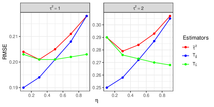
Refer to caption
Figure 5: Root mean square error (RMSE) for the proposed estimators. The x-axis stands for the sparsity level η\eta.
Table 7: Summary statistics for the EigenPrism-related estimators; n=p=300.n=p=300. Biases, standard errors (SE) and the root mean square errors (RMSE) of the different estimators, computed over 100100 independent datasets for each setting. The relative improvement over the EigenPrism estimator τ~2\tilde{\tau}^{2} (in terms of RMSE) is also shown. An estimate for the standard deviation of RMSE (σ^R​M​S​E\hat{\sigma}_{RMSE}) was calculated using the delta method.
η\eta τ2\tau^{2} Estimator Bias SE RMSE % Change σ^R​M​S​E\hat{\sigma}_{RMSE}
10% 1 τ~2\tilde{\tau}^{2} 0.01 0.204 0.204 0.00 0.014
10% 1 Tg~T_{\tilde{g}} 0.01 0.19 0.19 -6.86 0.012
10% 1 Th~T_{\tilde{h}} 0.01 0.204 0.203 -0.49 0.014
30% 1 τ~2\tilde{\tau}^{2} 0.01 0.202 0.201 0.00 0.014
30% 1 Tg~T_{\tilde{g}} 0.01 0.195 0.194 -3.48 0.014
30% 1 Th~T_{\tilde{h}} 0.01 0.201 0.201 0.00 0.014
50% 1 τ~2\tilde{\tau}^{2} 0.00 0.206 0.205 0.00 0.014
50% 1 Tg~T_{\tilde{g}} 0.00 0.202 0.201 -1.95 0.014
50% 1 Th~T_{\tilde{h}} 0.01 0.202 0.201 -1.95 0.015
70% 1 τ~2\tilde{\tau}^{2} 0.00 0.212 0.211 0.00 0.015
70% 1 Tg~T_{\tilde{g}} 0.00 0.209 0.208 -1.42 0.015
70% 1 Th~T_{\tilde{h}} 0.00 0.203 0.202 -4.27 0.015
90% 1 τ~2\tilde{\tau}^{2} -0.01 0.219 0.218 0.00 0.016
90% 1 Tg~T_{\tilde{g}} -0.01 0.218 0.218 0.00 0.016
90% 1 Th~T_{\tilde{h}} 0.00 0.204 0.203 -6.88 0.015
10% 2 τ~2\tilde{\tau}^{2} 0.00 0.291 0.29 0.00 0.020
10% 2 Tg~T_{\tilde{g}} 0.02 0.251 0.25 -13.79 0.016
10% 2 Th~T_{\tilde{h}} 0.01 0.291 0.29 0.00 0.020
30% 2 τ~2\tilde{\tau}^{2} 0.03 0.279 0.279 0.00 0.019
30% 2 Tg~T_{\tilde{g}} 0.03 0.258 0.258 -7.53 0.018
30% 2 Th~T_{\tilde{h}} 0.03 0.276 0.276 -1.08 0.019
50% 2 τ~2\tilde{\tau}^{2} 0.02 0.285 0.284 0.00 0.019
50% 2 Tg~T_{\tilde{g}} 0.01 0.273 0.272 -4.23 0.019
50% 2 Th~T_{\tilde{h}} 0.02 0.274 0.273 -3.87 0.020
70% 2 τ~2\tilde{\tau}^{2} 0.01 0.294 0.293 0.00 0.020
70% 2 Tg~T_{\tilde{g}} 0.00 0.289 0.287 -2.05 0.019
70% 2 Th~T_{\tilde{h}} 0.01 0.271 0.27 -7.85 0.019
90% 2 τ~2\tilde{\tau}^{2} -0.01 0.308 0.307 0.00 0.022
90% 2 Tg~T_{\tilde{g}} -0.01 0.307 0.305 -0.65 0.022
90% 2 Th~T_{\tilde{h}} 0.00 0.269 0.268 -12.7 0.019

3.7 Discussion and Future Work

In this work, we proposed a zero-estimator approach for improving estimation of the signal and noise levels explained by a set of covariates in a high-dimensional regression setting when the covariate distribution is known. We presented theoretical properties of the naive estimator τ^2,\hat{\tau}^{2}, and the proposed improved estimators Th^T_{\hat{h}} and Tg^T_{\hat{g}}. In a simulation study, we demonstrated that the zero-estimator approach leads to a significant reduction in the RMSE. Our method does not rely on sparsity assumptions of the regression coefficient vector, normality of the covariates, or linearity of E⁡(Y|X)E(Y|X). The goal in this work is to estimate the signal coming from the best linear function of the covariates, which is a model-free quantity. Our simulations demonstrate that our approach can be generalized to improve other estimators as well.

We suggest the following directions for future work. One natural extension is to relax the assumption of known covariate distribution to allow for a more general setting. This may be studied under the semi-supervised setting where one has access to a large amount of unlabeled data (N≫nN\gg n) in order to obtain theoretical results as a function of N.N. Another possible future research might be to extend the proposed approach to generalized linear models (GLM) such as logistic and Poisson regression, or survival models.

Supplementary Material

Proof of Proposition 3.1.


Let Wi=(Wi​1,…,Wi​p)T{W_{i}}={\left({{W_{i1}},...,{W_{ip}}}\right)^{T}} and notice that τ^2=1n⁡(n−1)​∑i1≠i2n∑j=1pWi1​j​Wi2​j\hat{\tau}^{2}=\frac{1}{{n\left({n-1}\right)}}\sum\limits_{{i_{1}}\neq{i_{2}}}^{n}\sum\limits_{j=1}^{p}{{W_{{i_{1}}j}}{W_{{i_{2}}j}}} is a U-statistic of order 2 with the kernel hτ​(W1,W2)=W1T​W2=∑j=1pW1​j​W2​j.h_{\tau}\left({{W_{1}},{W_{2}}}\right)=W_{1}^{T}{W_{2}}=\sum\limits_{j=1}^{p}{{W_{1j}}{W_{2j}}}.

By Theorem 12.3 in van der Vaart 2000,

Var​(τ^2)=4​(n−2)n⁡(n−1)​ζ1+2n⁡(n−1)​ζ2,{\text{Var}}\left({{{\hat{\tau}}^{2}}}\right)=\frac{{4\left({n-2}\right)}}{{n\left({n-1}\right)}}{\zeta_{1}}+\frac{2}{{n\left({n-1}\right)}}{\zeta_{2}}, (3.22)

where ζ1≡Cov​[h⁡(W1,W2),h⁡(W1,W~2)]{\zeta_{1}}\equiv{\text{Cov}}\left[{h\left({{W_{1}},{W_{2}}}\right),h\left({{W_{1}},{{\widetilde{W}_{2}}}}\right)}\right] and ζ2≡Var​[h⁡(W1,W2)],{\zeta_{2}}\equiv{\text{Var}}\left[{h\left({{W_{1}},{W_{2}}}\right)}\right], and where W~2\widetilde{W}_{2} is an independent copy of W2W_{2}. Define the p×pp\times p matrix 𝐀=E⁡(W​WT){\bf{A}}=E\left({{{W}}{W}^{T}}\right) and notice that

ζ1\displaystyle{\zeta_{1}} ≡Cov​[h⁡(W1,W2),h⁡(W1,W~2)]\displaystyle\equiv\text{Cov}\left[{h\left({{{W}_{1}},{{W}_{2}}}\right),h\left({{{W}_{1}},{{\widetilde{W}}_{2}}}\right)}\right]
=∑j,j′pCov​(W1​j​W2​j,W1​j′​W~2​j′)=∑j,j′p(βj​βj′​E​[W1​j​W1​j′]−βj2​βj′2)\displaystyle=\sum\limits_{j,j^{\prime}}^{p}{\text{Cov}\left({{W_{1j}}{W_{2j}},{W_{1j^{\prime}}}{{\widetilde{W}}_{2j^{\prime}}}}\right)}=\sum\limits_{j,j^{\prime}}^{p}{\left({{\beta_{j}}{\beta_{j^{\prime}}}E\left[{{W_{1j}}{W_{1j^{\prime}}}}\right]-\beta_{j}^{2}\beta_{j^{\prime}}^{2}}\right)}
=βT​𝐀​β−‖β‖4,\displaystyle={\beta^{T}}{\bf{A}}\beta-{\left\|\beta\right\|^{4}},

and

ζ2\displaystyle{\zeta_{2}} ≡Cov​[h⁡(W1,W2),h⁡(W1,W2)]\displaystyle\equiv{\text{Cov}}\left[{h\left({{{W}_{1}},{{W}_{2}}}\right),h\left({{{W}_{1}},{{W}_{2}}}\right)}\right]
=∑j,j′Cov​(W1​j​W2​j,W1​j′​W2​j′)=∑j,j′((E⁡[W1​j​W1​j′])2−βj2​βj′2)\displaystyle=\sum\limits_{j,j^{\prime}}{{\text{Cov}}\left({{W_{1j}}{W_{2j}},{W_{1j^{\prime}}}{W_{2j^{\prime}}}}\right)}=\sum\limits_{j,j^{\prime}}\left({{{\left({E\left[{{W_{1j}}{W_{1j^{\prime}}}}\right]}\right)}^{2}}-\beta_{j}^{2}\beta_{j^{\prime}}^{2}}\right)
=‖𝐀‖F2−‖β‖4,\displaystyle=\left\|{\bf{A}}\right\|_{F}^{2}-{\left\|\beta\right\|^{4}},

where ‖A‖F2\|\textbf{A}\|_{F}^{2} is the Frobenius norm of A.\textbf{A}. Thus, (2.6) follows from (3.22). ∎

Proof of Proposition 2.2.


Since τ^2\hat{\tau}^{2} is an unbiased estimator of τ2,\tau^{2}, then it is enough to prove that Var​[τ^2]→n→∞0\text{Var}[\hat{\tau}^{2}]\xrightarrow{n\rightarrow\infty}0. By (2.6) it is enough to require that βT​A​βn→n→∞0\frac{\beta^{T}\textbf{A}\beta}{n}\xrightarrow{n\rightarrow\infty}0 and ‖A‖F2n2→n→∞0\frac{\|\textbf{A}\|^{2}_{F}}{n^{2}}\xrightarrow{n\rightarrow\infty}0. The latter is assumed and we now show that the former also holds true.
Let λ1​𝐀≥…≥λp​𝐀\lambda_{1{\bf A}}\geq...\geq\lambda_{p{\bf A}} be the eigenvalues of A and notice that A is symmetric. Thus,

1n2​(λ1​𝐀)2≤1n2​∑j=1pλj​𝐀2=1n2​t​r​(A2)=1n2​‖A‖F2.\frac{1}{n^{2}}(\lambda_{1{\bf A}})^{2}\leq\frac{1}{n^{2}}\sum_{j=1}^{p}\lambda_{j{\bf A}}^{2}=\frac{1}{n^{2}}tr(\textbf{A}^{2})=\frac{1}{n^{2}}\|\textbf{A}\|_{F}^{2}.

Since we assume that ‖A‖F2n2→n→∞0\frac{\|\textbf{A}\|^{2}_{F}}{n^{2}}\xrightarrow{n\rightarrow\infty}0, we can conclude that λ1​𝐀n→n→∞0\frac{\lambda_{1{\bf A}}}{n}\xrightarrow{n\rightarrow\infty}0. Now, recall that the maximum of the quadratic form aT​𝐀​a{a^{T}}{\bf{A}}a satisfies λ1​𝐀=maxaaT​𝐀​a‖a‖2.{\lambda_{1{\bf A}}}=\mathop{\max}\limits_{a}\,\frac{{{a^{T}}{\bf{A}}a}}{{{{\left\|a\right\|}^{2}}}}. Hence,

1n​βT​A​β≡1n​‖β‖2​[(β‖β‖)T​A​β‖β‖]≤1n​‖β‖2​λ1=λ1n​τ2→n→∞0,\frac{1}{n}\beta^{T}\textbf{A}\beta\equiv\frac{1}{n}\|\beta\|^{2}[(\frac{\beta}{\|\beta\|})^{T}\textbf{A}\frac{\beta}{\|\beta\|}]\leq\frac{1}{n}\|\beta\|^{2}\lambda_{1}=\frac{\lambda_{1}}{n}\tau^{2}\xrightarrow{n\rightarrow\infty}0,

where the last limit follows from the assumption that τ2=O⁡(1),\tau^{2}=O(1), and from the fact that λ1n→n→∞0.\frac{\lambda_{1}}{n}\xrightarrow{n\rightarrow\infty}0.
We conclude that Var​[τ^2]→n→∞0\text{Var}[\hat{\tau}^{2}]\xrightarrow{n\rightarrow\infty}0. ∎

Proof of Proposition 3.3.


Recall that (3.8) states that σ^2≡σ^Y2−τ^2{\hat{\sigma}^{2}}\equiv\hat{\sigma}_{Y}^{2}-{\hat{\tau}^{2}}. Thus,

Var​(σ^2)=Var​(τ^2)+Var​(σ^Y2)−2​Cov​(σ^Y2,τ^2).\displaystyle\text{Var}\left({{{\hat{\sigma}}^{2}}}\right)=\text{Var}\left({{{\hat{\tau}}^{2}}}\right)+\text{Var}\left({\hat{\sigma}_{Y}^{2}}\right)-2\text{Cov}\left(\hat{\sigma}_{Y}^{2},{\hat{\tau}}^{2}\right). (3.23)

The variance of τ^2\hat{\tau}^{2} is given in (2.6). By standard U-statistic calculations (see e.g., Example 1.8 in Bose and Chatterjee 2018), the variance of σ^Y2\hat{\sigma}_{Y}^{2} is

Var​(σ^Y2)=4​(n−2)n⁡(n−1)​ψ1+2n⁡(n−1)​ψ2,\displaystyle\text{Var}(\hat{\sigma}_{Y}^{2})=\frac{4(n-2)}{n(n-1)}\psi_{1}+\frac{2}{n(n-1)}\psi_{2},

where ψ1≡μ4−σY44\psi_{1}\equiv\frac{\mu_{4}-\sigma_{Y}^{4}}{4} and ψ2≡μ4+σY42.\psi_{2}\equiv\frac{\mu_{4}+\sigma_{Y}^{4}}{2}. This can be further simplified to obtain

Var​(σ^Y2)=1n​μ4−(n−3)n⁡(n−1)​σY4.\displaystyle\text{Var}\left({\hat{\sigma}_{Y}^{2}}\right)=\frac{1}{n}{\mu_{4}}-\frac{{\left({n-3}\right)}}{{n\left({n-1}\right)}}\sigma_{Y}^{4}. (3.24)

We now calculate the covariance between and σ^Y2\hat{\sigma}_{Y}^{2} and τ^2.\hat{\tau}^{2}. Write,

Cov​(σ^Y2,τ^2)=Cov​[1n⁡(n−1)​∑i1≠i2(Yi1−Yi2)2/2,1n⁡(n−1)​∑j=1p∑i1≠i2Wi1​j​Wi2​j]\displaystyle\text{Cov}\left({\hat{\sigma}_{Y}^{2},{{\hat{\tau}}^{2}}}\right)=\text{Cov}\left[{\frac{1}{{n\left({n-1}\right)}}\sum\limits_{{i_{1}}\neq{i_{2}}}{{{\left({{Y_{{i_{1}}}}-{Y_{{i_{2}}}}}\right)}^{2}}/2,\frac{1}{{n\left({n-1}\right)}}\sum\limits_{j=1}^{p}{\sum\limits_{{i_{1}}\neq{i_{2}}}{{W_{{i_{1}}j}}{W_{{i_{2}}j}}}}}}\right]
=12​n2​(n−1)2​∑j=1p∑i1≠i2∑i3≠i4Cov​[Wi3​j​Wi4​j,(Yi1−Yi2)2].\displaystyle=\frac{1}{{2{n^{2}}{{\left({n-1}\right)}^{2}}}}\sum\limits_{j=1}^{p}{\sum\limits_{{i_{1}}\neq{i_{2}}}{\sum\limits_{{i_{3}}\neq{i_{4}}}{\text{Cov}\left[{{W_{{i_{3}}j}}{W_{{i_{4}}j}}},{{\left({{Y_{{i_{1}}}}-{Y_{{i_{2}}}}}\right)}^{2}}\right]}}}.

The covariance above is different from zero either when one of {i1,i2}\{i_{1},i_{2}\} is equal to one of {i3,i4}\{i_{3},i_{4}\}, or when {i1,i2}\{i_{1},i_{2}\} is equal to {i3,i4}\{i_{3},i_{4}\}. There are 4​n​(n−1)​(n−2)4n(n-1)(n-2) quadruples (i1,i2,i3,i4)(i_{1},i_{2},i_{3},i_{4}) for the first case, and 2​n​(n−1)2n(n-1) for the second case. Therefore,

Cov​[σ^Y2,τ^2]=2​(n−2)n⁡(n−1)​∑j=1pCov​[W1​j​W2​j,(Y−Y3)2]+1n⁡(n−1)​∑j=1pCov​[W1​j​W2​j,(Y1−Y2)2].\displaystyle\text{Cov}[\hat{\sigma}_{Y}^{2},\hat{\tau}^{2}]=\frac{2(n-2)}{n(n-1)}\sum_{j=1}^{p}\text{Cov}[W_{1j}{W_{2j}},(Y-Y_{3})^{2}]+\frac{1}{n(n-1)}\sum_{j=1}^{p}\text{Cov}[W_{1j}W_{2j},(Y_{1}-{Y_{2}})^{2}]. (3.25)

The first covariance term in (3.25) is

Cov​[W1​j​W2​j,(Y1−Y3)2]=E⁡([W1​j​W2​j−E⁡(W1​j)​E​(W2​j)]​[(Y1−Y3)2−2​σY2])\displaystyle\text{Cov}[W_{1j}W_{2j},(Y_{1}-Y_{3})^{2}]=E\Big([W_{1j}W_{2j}-E(W_{1j})E(W_{2j})][(Y_{1}-Y_{3})^{2}-2\sigma_{Y}^{2}]\Big)
=E⁡([W1​j​W2​j−βj2]​[(Y1−α−(Y3−α))2−2​σY2])\displaystyle=E\Big([W_{1j}W_{2j}-\beta_{j}^{2}][(Y_{1}-\alpha-(Y_{3}-\alpha))^{2}-2\sigma_{Y}^{2}]\Big)
=E⁡([W1​j​W2​j−βj2]​[{(Y1−α)2−σY2}−2​(Y1−α)​(Y3−α)+(Y3−α)2−σY2])\displaystyle=E\Big([W_{1j}W_{2j}-\beta_{j}^{2}][\{(Y_{1}-\alpha)^{2}-\sigma_{Y}^{2}\}-2(Y_{1}-\alpha)(Y_{3}-\alpha)+(Y_{3}-\alpha)^{2}-\sigma_{Y}^{2}]\Big)
=E⁡([W1​j​W2​j−βj2]​[{(Y1−α)2−σY2}])\displaystyle=E\Big([W_{1j}W_{2j}-\beta_{j}^{2}][\{(Y_{1}-\alpha)^{2}-\sigma_{Y}^{2}\}]\Big)
=E⁡[W1​j​(Y1−α)2]​βj2−βj2​σY2.\displaystyle=E\left[{{W_{1j}}{{\left({Y_{1}-\alpha}\right)}^{2}}}\right]\beta_{j}^{2}-\beta_{j}^{2}\sigma_{Y}^{2}.

The second covariance term of (3.25) is

Cov​[W1​j​W2​j,(Y1−Y2)2]=E⁡{[W1​j​W2​j−E⁡(W1​j​W2​j)]​[(Y1−Y2)2−E⁡{(Y1−Y2)2}]}\displaystyle\text{Cov}\left[{W_{1j}W_{2j},{{\left(Y_{1}-Y_{2}\right)}^{2}}}\right]=E\left\{{\left[{W_{1j}W_{2j}-E\left({W_{1j}W_{2j}}\right)}\right]\left[{{{\left(Y_{1}-Y_{2}\right)}^{2}}-E\left\{{{{\left(Y_{1}-Y_{2}\right)}^{2}}}\right\}}\right]}\right\}
=E⁡{(W1​j​W2​j−βj2)​[(Y1−Y2)2−2​σY2]}\displaystyle=E\left\{{\left({W_{1j}W_{2j}-\beta_{j}^{2}}\right)\left[{{{\left(Y_{1}-Y_{2}\right)}^{2}}-2\sigma_{Y}^{2}}\right]}\right\}
=E⁡{(W1​j​W2​j−βj2)​[{(Y1−α)−(Y2−α)}2−2​σY2]}\displaystyle=E\left\{{\left({W_{1j}W_{2j}-\beta_{j}^{2}}\right)\left[{{{\left\{{\left({Y_{1}-\alpha}\right)-\left({Y_{2}-\alpha}\right)}\right\}}^{2}}-2\sigma_{Y}^{2}}\right]}\right\}
=E⁡{(W1​j​W2​j−βj2)​[{(Y1−α)2−σY2}−2​(Y1−α)​(Y2−α)+{(Y2−α)2−σY2}]}\displaystyle=E\left\{{\left({W_{1j}W_{2j}-\beta_{j}^{2}}\right)\left[{\left\{{{{\left({Y_{1}-\alpha}\right)}^{2}}-\sigma_{Y}^{2}}\right\}-2\left({Y_{1}-\alpha}\right)\left({Y_{2}-\alpha}\right)+\left\{{{{\left({Y_{2}-\alpha}\right)}^{2}}-\sigma_{Y}^{2}}\right\}}\right]}\right\}
=2​E​{[(Y1−α)2−σY2]​(W1​j​W2​j−βj2)}−2​E​[(W1​j​W2​j−βj2)​(Y1−α)​(Y2−α)]\displaystyle=2E\left\{{\left[{{{\left({Y_{1}-\alpha}\right)}^{2}}-\sigma_{Y}^{2}}\right]\left({W_{1j}W_{2j}-\beta_{j}^{2}}\right)}\right\}-2E\left[{\left({W_{1j}W_{2j}-\beta_{j}^{2}}\right)\left({Y_{1}-\alpha}\right)\left({Y_{2}-\alpha}\right)}\right]
=2​{E⁡[(Y1−α)2​W1​j]​βj−σY2​βj2}−2​E​[W1​j​(Y1−α)​W2​j​(Y2−α)]\displaystyle=2\left\{{E\left[{{{\left({Y_{1}-\alpha}\right)}^{2}}{W_{1j}}}\right]{\beta_{j}}-\sigma_{Y}^{2}\beta_{j}^{2}}\right\}-2E\left[{{W_{1j}}\left({Y_{1}-\alpha}\right)W_{2j}\left({Y_{2}-\alpha}\right)}\right]
=2​E​[(Y1−α)2​W1​j]​βj−2​σY2​βj2−2​{E⁡[W1​j​(Y1−α)]}2,\displaystyle=2E\left[{{{\left({Y_{1}-\alpha}\right)}^{2}}{W_{1j}}}\right]{\beta_{j}}-2\sigma_{Y}^{2}\beta_{j}^{2}-2{\left\{{E\left[{{W_{1j}}\left({Y_{1}-\alpha}\right)}\right]}\right\}^{2}},

Hence, by (3.25) we have

Cov​(σ^Y2,τ^2)\displaystyle\text{Cov}\left({\hat{\sigma}_{Y}^{2},{{\hat{\tau}}^{2}}}\right) =2​(n−2)n⁡(n−1)​∑j=1p{E⁡[W1​j​(Y1−α)2]​βj−βj2​σY2}\displaystyle=\frac{{2\left({n-2}\right)}}{{n\left({n-1}\right)}}\sum\limits_{j=1}^{p}{\left\{{E\left[{W_{1j}{{\left({Y_{1}-\alpha}\right)}^{2}}}\right]{\beta_{j}}-\beta_{j}^{2}\sigma_{Y}^{2}}\right\}}
+1n⁡(n−1)∑j=1p{2E[(Y1−α)2W1​j]βj−2σY2βj2−2{E[W1​j(Y1−α)]}2},\displaystyle+\frac{1}{{n\left({n-1}\right)}}\sum\limits_{j=1}^{p}{\left\{{2E\left[{{{\left({Y_{1}-\alpha}\right)}^{2}}W_{1j}}\right]{\beta_{j}}-2\sigma_{Y}^{2}\beta_{j}^{2}-2{{\left\{{E\left[{W_{1j}\left({Y_{1}-\alpha}\right)}\right]}\right\}}^{2}}}\right\}},

which can be further simplified as

Cov​(σ^Y2,τ^2)=2n​(πT​β−τ2​σY2)−2n⁡(n−1)​∑j=1p{E⁡[W1​j​(Y1−α)]}2,\displaystyle\text{Cov}\left({\hat{\sigma}_{Y}^{2},{{\hat{\tau}}^{2}}}\right)=\frac{2}{n}\left({{\pi^{T}}\beta-{\tau^{2}}\sigma_{Y}^{2}}\right)-\frac{2}{{n\left({n-1}\right)}}\sum\limits_{j=1}^{p}{{{\left\{{E\left[{W_{1j}\left({Y_{1}-\alpha}\right)}\right]}\right\}}^{2}}}, (3.26)

where π=(π1,…,πp)T\pi={\left({{\pi_{1}},...,{\pi_{p}}}\right)^{T}} and πj≡E⁡[(Y1−α)2​W1​j]{\pi_{j}}\equiv E\left[{{{\left({Y_{1}-\alpha}\right)}^{2}}W_{1j}}\right].
Plugging (3.24) and (3.26) into (3.23) leads to (3.3). ∎

Proof of Corollary 3.1.


Since σ^2\hat{\sigma}^{2} is an unbiased estimator of σ2,\sigma^{2}, it is enough to prove that Var​(σ^2)→n→∞0.\text{Var}(\hat{\sigma}^{2})\xrightarrow{n\rightarrow\infty}~0. Recall that σ^2=σ^Y2−τ^2\hat{\sigma}^{2}=\hat{\sigma}^{2}_{Y}-\hat{\tau}^{2}. It follows that Var​(σ^2)≤2​Var​(σ^Y2)+2​Var​(τ^2)\text{Var}\left({{{\hat{\sigma}}^{2}}}\right)\leq 2\text{Var}\left({\hat{\sigma}_{Y}^{2}}\right)+2\text{Var}\left({{{\hat{\tau}}^{2}}}\right). Thus, it is enough to prove that Var​(σ^Y2)→n→∞0\text{Var}(\hat{\sigma}_{Y}^{2})\xrightarrow{n\rightarrow\infty}~0 and Var​(τ^2)→n→∞0.\text{Var}(\hat{\tau}^{2})\xrightarrow{n\rightarrow\infty}~0. The former requires, by (3.24), the assumption that μ4\mu_{4} is bounded and the latter holds true by Proposition 2.2. ∎

Remark 3.1.

The condition ‖𝐀‖F2n2→0\frac{\|{\bf A}\|_{F}^{2}}{n^{2}}\rightarrow 0 holds in the homoskedastic linear model with the additional assumption that the columns of 𝐗\bf{X} are independent (Livne et al. 2021, Proposition 2). We now show two more examples where the condition ‖𝐀‖F2n2→0\frac{\|{\bf A}\|_{F}^{2}}{n^{2}}\rightarrow 0 holds without assuming linearity.

1) We show that if p/n2→0p/n^{2}\rightarrow 0 and Y2≤CY^{2}\leq C for some constant CC, then ‖𝐀‖F2n2→0\frac{\|{\bf A}\|_{F}^{2}}{n^{2}}\rightarrow 0. For a∈ℝpa\in\mathbb{R}^{p} we have,

aT​𝐀​a\displaystyle{a^{T}}{\bf{A}}a =aT​E​(𝐖𝐖T)​a=E⁡(aT​𝐖𝐖T​a)=E⁡[(aT​𝐖)2]\displaystyle={a^{T}}E\left({{\bf{W}}{{\bf{W}}^{T}}}\right)a=E\left({{a^{T}}{\bf{W}}{{\bf{W}}^{T}}a}\right)=E\left[{{{\left({{a^{T}}{\bf{W}}}\right)}^{2}}}\right]
=E⁡[(Y​∑j=1paj​Xi​j)2]≤C​E​[(∑j=1paj​Xi​j)2]\displaystyle=E\left[{{{\left(Y{\sum\limits_{j=1}^{p}{{a_{j}}{X_{ij}}}}\right)}^{2}}}\right]\leq{C}E\left[{{{\left({\sum\limits_{j=1}^{p}{{a_{j}}{X_{ij}}}}\right)}^{2}}}\right]
=C⁡{∑j=1paj2​E⁡(Xi​j2)⏟1}+C​E​(∑j≠j′aj​aj′​E⁡(Xi​j​Xj′)⏟0)\displaystyle={C}\left\{{\sum\limits_{j=1}^{p}{a_{j}^{2}\underbrace{E\left({X_{ij}^{2}}\right)}_{1}}}\right\}+CE\left({\sum\limits_{j\neq j^{\prime}}{{a_{j}}{a_{j^{\prime}}}}\underbrace{E\left({{X_{ij}}{X_{j^{\prime}}}}\right)}_{0}}\right)
=C​‖a‖2,\displaystyle={C}{\left\|a\right\|^{2}}, (3.27)

where the last equality follows from Σ=𝐈.{\Sigma}={\bf I}. Now, let λ1​𝐀≥λ2𝐀≥,…,≥λp​𝐀𝐀\lambda_{1{\bf A}}\geq\lambda_{2}^{\bf A}\geq,...,\geq\lambda_{p{\bf A}}^{\bf A} be the eigenvalues of 𝐀,\bf{A}, and recall that the extrema of the quadratic form aT​𝐀​a{a^{T}}{\bf{A}}a satisfies λ1​𝐀=maxaaT​𝐀​a‖a‖2,{\lambda_{1{\bf A}}}=\mathop{\max}\limits_{a}\,\frac{{{a^{T}}{\bf{A}}a}}{{{{\left\|a\right\|}^{2}}}}, and hence by (3.1) we have λ1≤C.\lambda_{1}\leq C. Now, since p/n2→0p/n^{2}\rightarrow 0 by assumption, it follows that

‖𝐀‖F2n2=t​r​a​c​e​(𝐀2)n2=∑j=1pλj​𝐀2n2≤p​λ1​𝐀2n2≤p​C2n2→0.\frac{{\left\|{\bf{A}}\right\|_{F}^{2}}}{{{n^{2}}}}=\frac{{trace\left({{{\bf{A}}^{2}}}\right)}}{{{n^{2}}}}=\frac{{\sum\limits_{j=1}^{p}{\lambda_{j{\bf A}}^{2}}}}{{{n^{2}}}}\leq\frac{{p\lambda_{1{\bf A}}^{2}}}{{{n^{2}}}}\leq\frac{{p{C^{2}}}}{{{n^{2}}}}\to 0. (3.28)

2) We show that if p/n2→0p/n^{2}\rightarrow 0, E⁡(Y4),E⁡(Xi​j4)≤CE(Y^{4}),E(X_{ij}^{4})\leq C for j=1,…,pj=1,...,p and C≥1C\geq 1, and the columns of 𝐗\bf{X} are independent, then ‖𝐀‖F2n2→0\frac{\|{\bf A}\|_{F}^{2}}{n^{2}}\rightarrow 0. For a∈ℝpa\in\mathbb{R}^{p} we have by Cauchy–Schwarz,

aT​𝐀​a\displaystyle{a^{T}}{\bf{A}}a =E⁡[Yi2​(∑j=1paj​Xi​j)2]≤[E⁡(Yi4)]1/2​{E⁡[(∑j=1paj​Xi​j)4]}1/2\displaystyle=E\left[{Y_{i}^{2}{{\left({\sum\limits_{j=1}^{p}{{a_{j}}{X_{ij}}}}\right)}^{2}}}\right]\leq{\left[{E\left({Y_{i}^{4}}\right)}\right]^{1/2}}{\left\{{E\left[{{{\left({\sum\limits_{j=1}^{p}{{a_{j}}{X_{ij}}}}\right)}^{4}}}\right]}\right\}^{1/2}}
≤C1/2​{∑j1​j2​j3​j4aj1​aj2​aj3​aj4​E​(Xi​j1​Xi​j2​Xi​j3​Xi​j4)}1/2\displaystyle\leq{C^{1/2}}{\left\{{\sum\limits_{{j_{1}}{j_{2}}{j_{3}}{j_{4}}}{{a_{{j_{1}}}}{a_{{j_{2}}}}{a_{{j_{3}}}}{a_{{j_{4}}}}E\left({{X_{i{j_{1}}}}{X_{i{j_{2}}}}{X_{i{j_{3}}}}{X_{i{j_{4}}}}}\right)}}\right\}^{1/2}}
≤C1/2​{∑j=1paj4​E​(Xi​j4)+∑j≠j′aj2​aj′2​E​(Xi​j2)​E​(Xi​j′2)}1/2\displaystyle\leq{C^{1/2}}{\left\{{\sum\limits_{j=1}^{p}{a_{j}^{4}E\left({X_{ij}^{4}}\right)+\sum\limits_{j\neq j^{\prime}}{a_{j}^{2}a_{j^{\prime}}^{2}E\left({X_{ij}^{2}}\right)E\left({X_{ij^{\prime}}^{2}}\right)}}}\right\}^{1/2}}
≤C1/2​{C​∑j=1paj4+C​∑j≠j′aj2​aj′2}1/2\displaystyle\leq{C^{1/2}}{\left\{{C\sum\limits_{j=1}^{p}{a_{j}^{4}+C\sum\limits_{j\neq j^{\prime}}{a_{j}^{2}a_{j^{\prime}}^{2}}}}\right\}^{1/2}}
≤C​{∑j=1paj4+∑j≠j′aj2​aj′2}1/2=C​‖a‖2.\displaystyle\leq C{\left\{{\sum\limits_{j=1}^{p}{a_{j}^{4}+\sum\limits_{j\neq j^{\prime}}{a_{j}^{2}a_{j^{\prime}}^{2}}}}\right\}^{1/2}}=C{\left\|a\right\|^{2}}.

Notice that since that the columns of 𝐗\bf{X} are independent, the expectation E⁡(Xi​j1​Xi​j2​Xi​j3​Xi​j4)E\left({{X_{i{j_{1}}}}{X_{i{j_{2}}}}{X_{i{j_{3}}}}{X_{i{j_{4}}}}}\right) is not zero (up to permutation) when j1=j2j_{1}=j_{2} and j3=j4j_{3}=j_{4} or when j1=j2=j3=j4.j_{1}=j_{2}=j_{3}=j_{4}. Also notice we obtained the same result as in (3.1), and hence ‖𝐀‖F2n2→0\frac{\|{\bf A}\|_{F}^{2}}{n^{2}}\rightarrow 0 follows by the same arguments as in the previous example.

Remark 3.2.

Calculations for Equation 3.13:
Write,

Cov​(τ^2,Zg)\displaystyle\text{Cov}\left({{{\hat{\tau}}^{2}},Z_{g}}\right) =Cov​(1n⁡(n−1)​∑i1≠i2∑j=1pWi1​j​Wi2​j,1n​∑i=1ng⁡(Xi))\displaystyle=\text{Cov}\left({\frac{1}{{n\left({n-1}\right)}}\sum\limits_{{i_{1}}\neq{i_{2}}}{\sum\limits_{j=1}^{p}{{W_{{i_{1}}j}}{W_{{i_{2}}j}}}},\frac{1}{n}\sum\limits_{i=1}^{n}{g(X_{i})}}\right)
=1n2​(n−1)​∑i1≠i2∑j=1p∑i=1nE⁡(Wi1​j​Wi2​j​g​(Xi))\displaystyle=\frac{1}{{{n^{2}}\left({n-1}\right)}}\sum\limits_{{i_{1}}\neq{i_{2}}}{\sum\limits_{j=1}^{p}{\sum\limits_{i=1}^{n}{E\left({{W_{{i_{1}}j}}{W_{{i_{2}}j}}g(X_{i})}\right)}}}
=2n2​(n−1)​∑i1≠i2∑j=1pE⁡(Wi1​j​gi1)​E​(Wi2​j)\displaystyle=\frac{2}{{{n^{2}}\left({n-1}\right)}}\sum\limits_{{i_{1}}\neq{i_{2}}}{\sum\limits_{j=1}^{p}{E\left({{W_{{i_{1}}j}}{g_{{i_{1}}}}}\right)E\left({{W_{{i_{2}}j}}}\right)}}
=2n2​(n−1)​∑i1≠i2∑j=1pE⁡(Wi1​j​gi1)​βj\displaystyle=\frac{2}{{{n^{2}}\left({n-1}\right)}}\sum\limits_{{i_{1}}\neq{i_{2}}}{\sum\limits_{j=1}^{p}{E\left({{W_{{i_{1}}j}}{g_{{i_{1}}}}}\right){\beta_{j}}}}
=2n​βT​θg,\displaystyle=\frac{2}{n}\beta^{T}\theta_{g},

where θg=E⁡[W​g​(X)]{\theta_{g}}=E\left[{Wg\left(X\right)}\right]. Also notice that Var​(Zg)=Var​(1n​∑i=1ng⁡(Xi))=Var​(g​(X))n.\text{Var}\left(Z_{g}\right)=\text{Var}\left({\frac{1}{n}\sum\limits_{i=1}^{n}{g(X_{i})}}\right)=\frac{{\text{Var}\left({g(X)}\right)}}{n}. Thus, by (3.11) we get

cg∗=Cov​(τ^2,Zg)Var​(Zg)=2​βT​θgVar​(g​(X)).{c_{g}^{*}}=\frac{{{\text{Cov}}\left({{{\hat{\tau}}^{2}},Z_{g}}\right)}}{{\text{Var}\left({Z_{g}}\right)}}=\frac{2\beta^{T}\theta_{g}}{{\text{Var}\left({g(X)}\right)}}.
Proof of Proposition 3.4.


We wish to prove that n​[Th−Th^]​→𝑝​0.\sqrt{n}\left[T_{h}-T_{\hat{h}}\right]\overset{p}{\rightarrow}~0. Write,

n​(Th−Th^)=n​[(Th−Tf)+(Tf−Tf^)+(Tf^−Th^)].\sqrt{n}\left({{T_{h}}-{T_{\hat{h}}}}\right)=\sqrt{n}\left[{\left({{T_{h}}-{T_{f}}}\right)+\left({{T_{f}}-{T_{\hat{f}}}}\right)+\left({{T_{\hat{f}}}-{T_{\hat{h}}}}\right)}\right].

Thus, we need to show that

n​(Th−Tf)​→𝑝​0,\displaystyle\sqrt{n}\left({T_{h}-T_{f}}\right)\overset{p}{\rightarrow}0, (3.29)
n​(Tf^−Th^)​→𝑝​0,and\displaystyle\sqrt{n}\left({T_{\hat{f}}-T_{\hat{h}}}\right)\overset{p}{\rightarrow}~0,\text{and} (3.30)
n​(Tf−Tf^)​→𝑝​0,\displaystyle\sqrt{n}\left({T_{f}-T_{\hat{f}}}\right)\overset{p}{\rightarrow}0, (3.31)

The proofs of (3.29) and (3.30) are essentially the same as the proof of Proposition 5 in Livne et al. 2021. This is true since h⁡(X)​𝟙A=f⁡(X)​𝟙A,h(X)\mathbbm{1}_{A}=f(X)\mathbbm{1}_{A}, where AA denotes the event that the selection procedure δ\delta perfectly selects the set Θ\Theta, i.e., A≡{𝐒δ=Θ},A\equiv\left\{{{{\bf{S}}_{\delta}}=\Theta}\right\}, and 𝟙A\mathbbm{1}_{A} denotes the indicator of A.A.

We now wish to prove (3.31). Write,

n​[Tf^−Tf]=n​[τ^2−c^f∗​Zf−(τ^2−cf∗​Zf)]=n​Zf​(cf∗−c^f∗).\sqrt{n}\left[T_{\hat{f}}-T_{f}\right]=\sqrt{n}\left[{{{\hat{\tau}}^{2}}-{\hat{c}_{f}^{*}}Z_{f}-\left({{{\hat{\tau}}^{2}}-{c_{f}^{*}}Z_{f}}\right)}\right]={\sqrt{n}}Z_{f}{\left({{{c_{f}^{*}}}-{\hat{c}_{f}^{*}}}\right)}.

By Markov and Cauchy-Schwarz inequalities, it is enough to show that

P{|nZf(c^f∗−cf∗)|>ε}≤E⁡{|n​Zf​(c^f∗−cf∗)|}ε≤n​E​(Zf2)​E​[(c^f∗−cf∗)2]ε→0.P\left\{{\left|{\sqrt{n}Z_{f}\left({\hat{c}_{f}^{*}-c_{f}^{*}}\right)}\right|>\varepsilon}\right\}\leq\frac{{E\left\{{\left|{\sqrt{n}Z_{f}\left({\hat{c}_{f}^{*}-c_{f}^{*}}\right)}\right|}\right\}}}{\varepsilon}\leq\frac{{\sqrt{nE\left({Z_{f}^{2}}\right)E\left[{{{\left({\hat{c}_{f}^{*}-c_{f}^{*}}\right)}^{2}}}\right]}}}{\varepsilon}\rightarrow 0.

Notice that E⁡(Zf2)=Var​(Zf)=Var​[f​(X)]nE(Z_{f}^{2})=\text{Var}(Z_{f})=\frac{\text{Var}[f(X)]}{n} and E⁡[(c^f∗−cf∗)2]=Var​(c^f∗),E[(\hat{c}_{f}^{*}-c_{f}^{*})^{2}]=\text{Var}(\hat{c}_{f}^{*}), where by (3.4) we have

c^f∗=2n⁡(n−1)​∑i1≠i2Wi1T​Wi2​f​(Xi2)Var​[f​(X)]≡UVar​[f​(X)].\hat{c}_{f}^{*}=\frac{{\frac{2}{{n\left({n-1}\right)}}\sum\limits_{{i_{1}}\neq{i_{2}}}{W_{{i_{1}}}^{T}{W_{{i_{2}}}}f\left({{X_{{i_{2}}}}}\right)}}}{{\text{Var}\left[{f\left(X\right)}\right]}}\equiv\frac{U}{\text{Var}[f(X)]}.

Hence, it enough to show that

Var​(U)Var​[f​(X)]→0.\frac{{\text{Var}\left(U\right)}}{{\text{Var}[f(X)]}}\rightarrow 0. (3.32)

The variance of UU is

Var​(U)\displaystyle\text{Var}(U) =Var​[2n⁡(n−1)​∑i1≠i2∑j=1pWi1​j​Wi2​j​f​(Xi2)]\displaystyle=\text{Var}\left[{\frac{2}{{n\left({n-1}\right)}}\sum\limits_{{i_{1}}\neq{i_{2}}}{\sum\limits_{j=1}^{p}{{W_{{i_{1}}j}}{W_{{i_{2}}j}}f(X_{i_{2}})}}}\right]
=4n2​(n−1)2​∑j,j′p∑i1≠i2,i3≠i4Cov​[Wi1​j​Wi2​j​f​(Xi2),Wi3​j′​Wi4​j′​f​(Xi4)].\displaystyle=\frac{4}{{{n^{2}}{{\left({n-1}\right)}^{2}}}}\sum\limits_{j,j^{\prime}}^{p}{\sum\limits_{{i_{1}}\neq{i_{2}},{i_{3}}\neq{i_{4}}}{\text{Cov}\left[{{W_{{i_{1}}j}}{W_{{i_{2}}j}}f(X_{i_{2}}),{W_{{i_{3}}j^{\prime}}}{W_{{i_{4}}j^{\prime}}}f(X_{i_{4}})}\right].}} (3.33)

The covariance in (Supplementary Material) is different from zero in the following two cases:

  1. 1.

    When {i1,i2}\left\{{{i_{1}},{i_{2}}}\right\} is equal to {i3,i4}.\left\{{{i_{3}},{i_{4}}}\right\}.

  2. 2.

    When one of {i1,i2}\left\{{{i_{1}},{i_{2}}}\right\} equals to {i3,i4}\left\{{{i_{3}},{i_{4}}}\right\} while the other is different.

The first condition includes two different sub-cases and each of those consists of n⁡(n−1)n(n-1) quadruples (i1,i2,i3,i4)(i_{1},i_{2},i_{3},i_{4}) that satisfy the condition. Similarly, the second condition above includes four different sub-cases and each of those consists of n​(n−1)​(n−2)n(n-1)(n-2) quadruples that satisfy the condition.

We now calculate the covariance for all these six sub-cases.
(1) The covariance when i1=i3,i2=i4{i_{1}}={i_{3}},{i_{2}}={i_{4}} is

Cov​[Wi1​j​Wi2​j​f​(Xi2),Wi1​j′​Wi2​j′​f​(Xi2)]\displaystyle\text{Cov}\left[{{W_{i_{1}j}}{W_{i_{2}j}}f(X_{i_{2}}),{W_{i_{1}j^{\prime}}}{{W_{i_{2}j^{\prime}}}}f(X_{i_{2}})}\right] =E⁡(Wi1​j​Wi1​j′)​E​[Wi2​j​Wi2​j′​f2​(Xi2)]\displaystyle=E\left({{W_{i_{1}j}}{W_{i_{1}j^{\prime}}}}\right)E\left[{{W_{i_{2}j}}{{W_{i_{2}j^{\prime}}}}f^{2}(X_{i_{2}})}\right]
−E⁡(Wi1​j)​E​[Wi2​j​f​(Xi2)]​E​(Wi1​j′)​E​[Wi2​j′​f​(Xi2)]\displaystyle-E({{W_{i_{1}j}}})E\left[{{W_{i_{2}j}}f(X_{i_{2}})}\right]E\left({{{W_{i_{1}j^{\prime}}}}}\right)E\left[{{{W_{i_{2}j^{\prime}}}}f(X_{i_{2}})}\right]
=E⁡(Wi1​j​Wi1​j′)​E​[Wi2​j​Wi2​j′​f2​(Xi2)]−βj​βj′​θf​j​θf​j′,\displaystyle=E\left({{W_{i_{1}j}}{W_{i_{1}j^{\prime}}}}\right)E\left[{{W_{i_{2}j}}{{W_{i_{2}j^{\prime}}}}f^{2}(X_{i_{2}})}\right]-{\beta_{j}}{\beta_{j^{\prime}}}{\theta_{fj}}{\theta_{fj^{\prime}}},

where recall that b≡W​f​(X).b\equiv Wf(X). Thus, we define

δ1≡∑j,j′{E⁡(Wi1​j​Wi1​j′)​E​[Wi2​j​Wi2​j′​f2​(Xi2)]−βj​βj′​θf​j​θf​j′}=E⁡(bT​𝐀​b)−(βT​θb)2.{\delta_{1}}\equiv\sum\limits_{j,j^{\prime}}{\left\{{E\left({{W_{i_{1}j}}{W_{i_{1}j^{\prime}}}}\right)E\left[{{W_{i_{2}j}}{W_{i_{2}j^{\prime}}}{f^{2}(X_{i_{2}})}}\right]-{\beta_{j}}{\beta_{j^{\prime}}}{\theta_{fj}}{\theta_{fj^{\prime}}}}\right\}}=E\left({{b^{T}}{\bf{A}}b}\right)-{\left({{\beta^{T}}\theta_{b}}\right)^{2}}. (3.34)

(2) The covariance when i1=i4,i2=i3{i_{1}}={i_{4}},{i_{2}}={i_{3}} is

Cov​[Wi1​j​Wi2​f​(Xi2),Wi2​j′​Wi1​j′​f​(Xi1)]\displaystyle\text{Cov}\left[{{W_{i_{1}j}}{W_{i_{2}}}f(X_{i_{2}}),{{W_{i_{2}j^{\prime}}}}{W_{i_{1}j^{\prime}}}f(X_{i_{1}})}\right] =E⁡[Wi1​j​Wi1​j′​f​(Xi1)]​E​[Wi2​j​Wi2​j′​f​(Xi2)]\displaystyle=E\left[{{W_{i_{1}j}}{W_{i_{1}j^{\prime}}}f(X_{i_{1}})}\right]E\left[{{W_{i_{2}j}}{{W_{i_{2}j^{\prime}}}}f(X_{i_{2}})}\right]
−E⁡(Wi1​j)​E​[Wi2​j​f​(Xi2)]​E​(Wi2​j′)​E​[Wi1​j′​f​(Xi1)]\displaystyle-E(W_{i_{1}j})E\left[{{{W_{i_{2}j}}}f(X_{i_{2}})}\right]E\left({{{W_{i_{2}j^{\prime}}}}}\right)E\left[{{W_{i_{1}j^{\prime}}}f(X_{i_{1}})}\right]
={E⁡[Wi​j​Wi​j′​f​(Xi)]}2−βj​βj′​θf​j​θf​j′.\displaystyle={\left\{{E\left[{{W_{ij}}{W_{ij^{\prime}}}f(X_{i})}\right]}\right\}^{2}}-{\beta_{j}}{\beta_{j^{\prime}}}{\theta_{fj}}{\theta_{fj^{\prime}}}.

Thus, we define

δ2≡∑j,j′{[E⁡(Wi​j​Wi​j′​f​(Xi))]2−βj​βj′​θf​j​θf​j′}=‖𝐁‖F2−(βT​θb)2,{\delta_{2}}\equiv\sum\limits_{j,j^{\prime}}{\left\{{{{\left[{E\left({{W_{ij}}{W_{ij^{\prime}}}f\left(X_{i}\right)}\right)}\right]}^{2}}-{\beta_{j}}{\beta_{j^{\prime}}}{\theta_{fj}}{\theta_{fj^{\prime}}}}\right\}}=\left\|{\bf{B}}\right\|_{F}^{2}-{\left({{\beta^{T}}\theta_{b}}\right)^{2}}, (3.35)

where 𝐁≡E⁡(W​WT​f​(X)).{\bf{B}}\equiv E\left({W{W^{T}}f\left(X\right)}\right).
(3) Similarly, when i1=i3,i2≠i4\,{i_{1}}={i_{3}},{i_{2}}\neq{i_{4}} we have

δ3≡∑j,j′{[E⁡(Wi​j​Wi​j′)​θf​j​θf​j′]−βj​βj′​θf​j​θf​j′}=θbT​𝐀​θb−(βT​θb)2.{\delta_{3}}\equiv\sum\limits_{j,j^{\prime}}{\left\{{\left[{E\left({{W_{ij}}{W_{ij^{\prime}}}}\right){\theta_{fj}}{\theta_{fj^{\prime}}}}\right]-{\beta_{j}}{\beta_{j^{\prime}}}{\theta_{fj}}{\theta_{fj^{\prime}}}}\right\}}={\theta_{b}^{T}}{\bf{A}}\theta_{b}-{\left({{\beta^{T}}\theta_{b}}\right)^{2}.} (3.36)

(4)-(5) When i1=i4,i2≠i3i_{1}=i_{4},i_{2}\neq i_{3} or when i2=i3,i1≠i4i_{2}=i_{3},i_{1}\neq i_{4} we have

δ4=δ5≡∑j,j′{θf​j​βj′​E​[Wi​j​Wi​j′​f​(Xi)]−βj​βj′​θf​j​θf​j′}=βT​𝐁​θb−(βT​θb)2.{\delta_{4}}=\delta_{5}\equiv\sum\limits_{j,j^{\prime}}{\left\{{{\theta_{fj}}{\beta_{j^{\prime}}}E\left[{{W_{ij}}{W_{ij^{\prime}}}f\left(X_{i}\right)}\right]-{\beta_{j}}{\beta_{j^{\prime}}}{\theta_{fj}}{\theta_{fj^{\prime}}}}\right\}}={\beta^{T}}{\bf{B}}\theta_{b}-{\left({{\beta^{T}}\theta_{b}}\right)^{2}.} (3.37)

(6) When i2=i4,i1≠i3i_{2}=i_{4},i_{1}\neq i_{3},

δ6≡∑j,j′{βj​βj′​E​[Wi​j​Wi​j′​f2​(Xi)]−βj​βj′​θf​j​θf​j′}=βT​𝐂​β−(βT​θb)2,{\delta_{6}}\equiv\sum\limits_{j,j^{\prime}}{\left\{{{\beta_{j}}{\beta_{j^{\prime}}}E\left[{{W_{ij}}{W_{ij^{\prime}}}{f^{2}(X_{i})}}\right]-{\beta_{j}}{\beta_{j^{\prime}}}{\theta_{fj}}{\theta_{fj^{\prime}}}}\right\}}={\beta^{T}}{\bf{C}}\beta-{\left({{\beta^{T}}\theta_{b}}\right)^{2}}, (3.38)

where 𝐂=E⁡(W​WT​f2​(X)).{\bf{C}}=E\left({W{W^{T}}f^{2}{{\left(X\right)}}}\right). Thus, plugging-in (3.34) - (3.38) into (Supplementary Material) gives

Var​(U)=4​{1n⁡(n−1)​(δ1+δ2)+(n−2)n⁡(n−1)​(δ3+δ4+δ5+δ6)}.\text{Var}\left(U\right)=4{\left\{{\frac{1}{{n\left({n-1}\right)}}\left({{\delta_{1}}+{\delta_{2}}}\right)+\frac{{\left({n-2}\right)}}{{n\left({n-1}\right)}}\left({{\delta_{3}}+{\delta_{4}}+{\delta_{5}}+{\delta_{6}}}\right)}\right\}}. (3.39)

Recall that we wish to show that Var​(U)Var​[f​(X)]→0.\frac{\text{Var}(U)}{\text{Var}[f(X)]}\rightarrow 0. Thus, it is enough to show that

(δ1+δ2)n2​Var​[f⁡(X)]→0,{\frac{{\left({{\delta_{1}}+{\delta_{2}}}\right)}}{{{n^{2}\text{Var}[f(X)]}}}}\to 0, (3.40)

and

(δ3+δ4+δ5+δ6)n​Var​[f⁡(X)]→0.{\frac{{\left({{\delta_{3}}+{\delta_{4}}+{\delta_{5}}+{\delta_{6}}}\right)}}{{{n\text{Var}[f(X)]}}}}\to 0. (3.41)

Consider δ1.\delta_{1}. For any square matrix 𝐌,{\bf M}, we denote λ1​𝐌{\lambda_{1{\bf{M}}}} to be the largest eigenvalue of 𝐌.{\bf M}. Write,

δ1n2​Var​[f⁡(X)]≤E⁡(bT​𝐀​b)n2​Var​[f⁡(X)]≤λ1​𝐀n​E⁡(‖b‖2)n​Var​[f⁡(X)]≤‖𝐀‖F2n2​E⁡(‖b‖2)n​Var​[f⁡(X)]→0,\frac{{{\delta_{1}}}}{{{n^{2}}\text{Var}\left[{f\left(X\right)}\right]}}\leq\frac{{E\left({{b^{T}}{\bf{A}}b}\right)}}{{{n^{2}}\text{Var}[f(X)]}}\leq\frac{{{\lambda_{1{\bf{A}}}}}}{n}\frac{{E\left({{{\left\|b\right\|}^{2}}}\right)}}{{n\text{Var}[f(X)]}}\leq\sqrt{\frac{{\left\|{\bf{A}}\right\|_{F}^{2}}}{{{n^{2}}}}}\frac{{E\left({{{\left\|b\right\|}^{2}}}\right)}}{{n\text{Var}[f(X)]}}\to 0,

where the last inequality holds since we assume that ‖𝐀‖F2n2→0\frac{{\left\|{\bf{A}}\right\|_{F}^{2}}}{{{n^{2}}}}\to 0 and E⁡(‖b‖2)n​Var​[f⁡(X)]\frac{{E\left({{{\left\|b\right\|}^{2}}}\right)}}{{n\text{Var}[f(X)]}} is bounded. Similarly,

δ2n2​Var​[f⁡(X)]≤‖𝐁‖F2n2​Var​[f⁡(X)]→0,\frac{{{\delta_{2}}}}{{{n^{2}}\text{Var}[f(X)]}}\leq\frac{{\left\|{\bf{B}}\right\|_{F}^{2}}}{{{n^{2}}\text{Var}[f(X)]}}\to 0,

where ‖𝐁‖F2n2​Var​[f⁡(X)]→0\frac{{\left\|{\bf{B}}\right\|_{F}^{2}}}{{{n^{2}\text{Var}[f(X)]}}}\to 0 by assumption.
Consider now δ3.\delta_{3}. Write,

δ3n​Var​[f⁡(X)]≤θbT​𝐀​θbn​Var​[f⁡(X)]≤λ1​𝐀n​‖θb‖2Var​[f​(X)]≤‖𝐀‖F2n2​‖θb‖2Var​[f​(X)]→0,\frac{{{\delta_{3}}}}{{n\text{Var}[f(X)]}}\leq\frac{{{\theta_{b}^{T}}{\bf{A}}\theta_{b}}}{{n\text{Var}[f(X)]}}\leq\frac{{{\lambda_{1{\bf{A}}}}}}{n}\frac{{{{\left\|\theta_{b}\right\|}^{2}}}}{{\text{Var}[f(X)]}}\leq\sqrt{\frac{{\left\|{\bf{A}}\right\|_{F}^{2}}}{{{n^{2}}}}}\frac{{{{\left\|\theta_{b}\right\|}^{2}}}}{{\text{Var}[f(X)]}}\to 0,

where the above holds since we assume that ‖θb‖2Var​[f​(X)]\frac{\|\theta_{b}\|^{2}}{\text{Var}[f(X)]} is bounded and ‖𝐀‖F2n2→0.\frac{{\left\|{\bf{A}}\right\|_{F}^{2}}}{{{n^{2}}}}\to 0.

Recall that δ4=δ5.\delta_{4}=\delta_{5}. By the Cauchy–Schwarz inequality and the inequality of arithmetic means we have

δ4n​Var​[f⁡(X)]≤βT​𝐁​θbn​Var​[f⁡(X)]≤|λ1​𝐁|n​‖β‖​‖θb‖Var​[f​(X)]≤‖𝐁‖F2n2​(‖β‖2+‖θb‖2)2​n​Var​[f⁡(X)]→0,\frac{{{\delta_{4}}}}{{n\text{Var}[f(X)]}}\leq\frac{{{\beta^{T}}{\bf{B}}\theta_{b}}}{{n\text{Var}[f(X)]}}\leq\frac{{\left|{{\lambda_{1{\bf{B}}}}}\right|}}{n}\frac{{\left\|\beta\right\|\left\|\theta_{b}\right\|}}{{\text{Var}[f(X)]}}\leq\sqrt{\frac{{\left\|{\bf{B}}\right\|_{F}^{2}}}{{{n^{2}}}}}\frac{{\left({{{\left\|\beta\right\|}^{2}}+{{\left\|\theta_{b}\right\|}^{2}}}\right)}}{{2n\text{Var}[f(X)]}}\rightarrow 0, (3.42)

where the expression in (3.42) converges to zero by similar same arguments as shown above.
Similarly for δ6,\delta_{6},

δ6n​Var​[f⁡(X)]≤βT​𝐂​βn​Var​[f⁡(X)]≤λ1​𝐂n​‖β‖2Var​[f​(X)]≤‖𝐂‖F2{n​Var​[f⁡(X)]}2​‖β‖2→0,\frac{{{\delta_{6}}}}{{n\text{Var}[f(X)]}}\leq\frac{{{\beta^{T}}{\bf{C}}\beta}}{{n\text{Var}[f(X)]}}\leq\frac{{{\lambda_{1{\bf{C}}}}}}{n}\frac{{{{\left\|\beta\right\|}^{2}}}}{{\text{Var}[f(X)]}}\leq\sqrt{\frac{{\left\|{\bf{C}}\right\|_{F}^{2}}}{{{\{n\text{Var}[f(X)]\}^{2}}}}}\|\beta\|^{2}\to 0,

where ‖𝐂‖F2{n​Var​[f⁡(X)]}2→0\frac{{\left\|{\bf{C}}\right\|_{F}^{2}}}{{\{n\text{Var}[f(X)]\}^{2}}}\to 0 and τ2≡‖β‖2=O⁡(1)\tau^{2}\equiv\|\beta\|^{2}=O(1) by assumptions. Hence, (3.32) follows. This completes the proof that n​[Th^−Th]​→𝑝​0.\sqrt{n}\left[T_{\hat{h}}-T_{h}\right]\overset{p}{\rightarrow}~0. ∎

Remark 3.3.

We first show that if Y2Y^{2} and Xi​j2X_{ij}^{2} are bounded for all j=1,…,pj=1,...,p, i=1,…,ni=1,...,n and p/n=O⁡(1)p/n=O(1), then E⁡(‖b‖2)n​Var​[f⁡(X)]\frac{{E\left({{{\left\|b\right\|}^{2}}}\right)}}{{n\text{Var}[f(X)]}} is bounded. Let CC be the upper bound of the maximum of Y2Y^{2} and Xi​j2X_{ij}^{2}, for j=1,…,pj=1,...,p and i=1,…,n.i=1,...,n. Then,

E⁡(‖b‖2)n​Var​[f⁡(X)]=∑j=1pE⁡(bj2)n​E​[f2​(X)]=∑j=1pE⁡[X1​j2​Y2​f2​(X)]n​E​[f2​(X)]≤C2​p​E​[f2​(X)]n​E​[f2​(X)]=C2​pn=O⁡(1),\frac{{E\left({{{\left\|b\right\|}^{2}}}\right)}}{{n\text{Var}\left[{f\left(X\right)}\right]}}=\frac{{\sum\limits_{j=1}^{p}{E\left({b_{j}^{2}}\right)}}}{{nE\left[{{f^{2}}\left(X\right)}\right]}}=\frac{{\sum\limits_{j=1}^{p}{E\left[{X_{1j}^{2}{Y^{2}}{f^{2}}\left({{X}}\right)}\right]}}}{{nE\left[{{f^{2}}\left(X\right)}\right]}}\leq\frac{{{C^{2}}pE\left[{{f^{2}}\left(X\right)}\right]}}{{nE\left[{{f^{2}}\left(X\right)}\right]}}=\frac{{{C^{2}}p}}{n}=O(1),

where notice that we used the assumption that p/n=O⁡(1).p/n=O(1).

We now show that under the same assumptions as above, together with the assumptions that Θ\Theta is bounded and Var​[f​(X)]≥c>0\text{Var}[f(X)]\geq c>0, then ‖𝐁‖F2n2​Var​[f⁡(X)]→0.\frac{{\left\|{\bf{B}}\right\|_{F}^{2}}}{{{n^{2}\text{Var}[f(X)]}}}\to 0. Recall that f⁡(X)=∑j<j′Xi​j​Xi​j′.f\left({{X}}\right)=\sum\limits_{j<j^{\prime}}{{X_{ij}}{X_{ij^{\prime}}}}. Notice that when Θ\Theta is bounded, and when the covariates Xi​jX_{ij}, i=1,…,ni=1,...,n, j=1,…,pj=1,...,p are bounded, then so is f⁡(X)f(X). Let CC be the upper bound of |f⁡(X)||f(X)|. Similarly to (3.1), for a∈ℝpa\in\mathbb{R}^{p}, we have

aT​𝐁​a\displaystyle{a^{T}}{\bf{B}}a =E⁡[aT​W​WT​a​f​(X)]≤E⁡[|f⁡(X)|​(aT​W)2]≤C​E​[(aT​X​Y)2]\displaystyle=E\left[{{a^{T}}W{W^{T}}af\left(X\right)}\right]\leq E\left[{\left|{f\left(X\right)}\right|{{\left({{a^{T}}W}\right)}^{2}}}\right]\leq CE\left[{{{\left({{a^{T}}XY}\right)}^{2}}}\right]
=C​E​[Y2​(∑j=1paj​Xj)2]≤C2​E​[(∑j=1paj​Xj)2]\displaystyle=CE\left[{{Y^{2}}{{\left({\sum\limits_{j=1}^{p}{{a_{j}}{X_{j}}}}\right)}^{2}}}\right]\leq{C^{2}}E\left[{{{\left({\sum\limits_{j=1}^{p}{{a_{j}}{X_{j}}}}\right)}^{2}}}\right]
=C2​∑j≠j′aj​aj′​E⁡(Xj​Xj′)⏟0+C2​∑j=1paj2​E​(Xj2)=C2​‖a‖2.\displaystyle={C^{2}}\sum\limits_{j\neq j^{\prime}}{{a_{j}}{a_{j^{\prime}}}\underbrace{E\left({{X_{j}}{X_{j^{\prime}}}}\right)}_{0}}+{C^{2}}\sum\limits_{j=1}^{p}{a_{j}^{2}E\left({X_{j}^{2}}\right)}={C^{2}}{\left\|a\right\|^{2}}. (3.43)

It follows that λ1​𝐁≤C2​‖a‖2‖a‖2=C2,{\lambda_{1{\bf{B}}}}\leq\frac{{{C^{2}}{{\left\|a\right\|}^{2}}}}{{{{\left\|a\right\|}^{2}}}}={C^{2}}, and by a similar argument as in (3.28) we conclude that

‖𝐁‖F2n2​Var​[f⁡(X)]≤p​λ1​𝐁2n2​Var​[f⁡(X)]≤p​C4n2​c→0,\frac{{\left\|{\bf{B}}\right\|_{F}^{2}}}{{{n^{2}\text{Var}[f(X)]}}}\leq\frac{{p\lambda_{1{\bf{B}}}^{2}}}{{{n^{2}\text{Var}[f(X)]}}}\leq\frac{pC^{4}}{{{n^{2}c}}}\to 0,

where recall we assume that n/p=O⁡(1)n/p=O(1). A similar argument can be used to show that under the above conditions, ‖𝐂‖F2{n​Var​[f⁡(X)]}2→0.\frac{{\left\|{\bf{C}}\right\|_{F}^{2}}}{{{\{n\text{Var}[f(X)]\}^{2}}}}\to 0.

Remark 3.4.

We use the the following simple selection procedure δ\delta:

Input: A dataset (𝐗n×p,𝐘n×1)\left({{{\bf{X}}_{n\times p}},{{\bf{Y}}_{n\times 1}}}\right).
  1. 1.

    Calculate β^12,…,β^p2\hat{\beta}_{1}^{2},...,\hat{\beta}_{p}^{2} where β^j2\hat{\beta}_{j}^{2} is given in (2.4) for j=1,…,p.j=1,...,p.

  2. 2.

    Calculate the differences λj=β^(j)2−β^(j−1)2{\lambda_{j}}=\hat{\beta}_{\left(j\right)}^{2}-\hat{\beta}_{\left({j-1}\right)}^{2} for j=2,…,pj=2,\ldots,p where β^(1)2<β^(2)2<…<β^(p)2\hat{\beta}_{\left(1\right)}^{2}<\hat{\beta}_{\left(2\right)}^{2}<...<\hat{\beta}_{\left(p\right)}^{2} denotes the order statistics.

  3. 3.

    Select the covariates 𝐒δ={j:β^(j)2>β^(j∗)2}{{\bf{S}}_{\delta}}=\left\{{j:\hat{\beta}_{\left(j\right)}^{2}>\hat{\beta}_{\left({{j^{*}}}\right)}^{2}}\right\}, where j∗=arg⁡maxj⁡λj{j^{*}}=\mathop{\arg\max}\limits_{j}{\lambda_{j}}.

Output: Return 𝐒δ{{\bf{S}}_{\delta}}.
Algorithm 7 Covariate selection δ\delta

The algorithm above finds the largest gap between the ordered estimated squared coefficients and then uses this gap as a threshold to select a set of coefficients 𝐒δ⊂{1,…,p}.{{\bf{S}}_{\delta}}\subset\left\{{1,...,p}\right\}. The algorithm works well in scenarios where a relatively large gap truly separates between larger coefficients and the smaller coefficients of the vector β\beta.

4 Real Data Application

In this chapter, we use the methods proposed in the previous chapters to estimate the signal level τ2\tau^{2} on different datasets. In real-world data (on opposed to synthetic data), it is common to encounter undesired issues such as error of measurements, outliers, highly-skewed covariates, collinear covariates, violation of the i.i.d. assumption, etc. In practice, these issues might impact the performance of the proposed estimators. Moreover, the theoretical results provided is this thesis are based on the underlying assumption that the covariates’ distribution is known, while in practice one needs to estimate it by using the unlabeled data. Our aim now in this chapter is to investigate how well our proposed estimators perform on real datasets.

We provide below a brief description of the four real datasets and the synthetic data we used in our simulations in this chapter. Data pre-possessing steps that were applied are also described.

  1. 1.

    The Blog Feedback dataset, which is publicly available at the UCI machine learning repository (https://archive.ics.uci.edu/ml/datasets/BlogFeedback), contains data from Hungarian blog sites. The covariates include blog posts characteristics such as: the number of comments in different time intervals relative to the publication of the blog post, and the length of the blog post. The response variable is the number of comments that a given blog post received within the first 24 hours after publication. A log transformation was applied to the response variable. The dataset includes N=122,993N=122,993 rows and 281 columns. After we removed collinear columns the resulting number of covariates was p=248.p=248.

  2. 2.

    The House Price dataset, which is publicly available at Kaggle (https://www.kaggle.com/datasets/egebozoglu/house-price-linear-regression), contains different house characteristics such as: number of bedrooms, square feet of different areas in the house, the number of years since renovation. The response variable is the house price. The dataset includes N=12,613N=12,613 rows and 21 columns. We also included all the pairwise interaction terms. The resulting number of covariates after removing collinear columns is p=138.p=138.

  3. 3.

    The Life Expectancy dataset, which is publicly available from Kaggle (https://www.kaggle.com/datasets/kumarajarshi/life-expectancy-who), consists of health, economic and social factors that affect life expectancy. The data was collected by the World Health Organization (WHO) between the years 2000 to 2015 for 193 countries. The covariates include information such as immunization level for Polio, the gross domestic product (GDP) and alcohol consumption level. The response variable is life expectancy in a given country in a given year. The dataset includes N=2,928N=2,928 rows and 22 columns. We also included all the pairwise interaction terms. The resulting number of covariates after removing collinear columns is p=190.p=190.

  4. 4.

    The Superconductivty dataset, which is publicly available at the UCI machine learning repository (https://archive.ics.uci.edu/ml/datasets/superconductivty+data), contains characteristics of superconducting materials (materials that conduct current with zero resistance). The covariates are based on properties such as atomic mass and radius, electron affinity and fusion heat. The response variable is the superconducting critical temperature. A log transformation was applied to the response variable. The dataset includes N=21,263N=21,263 rows and 8181 columns. We also included the pairwise interactions terms of the top ten covariates that have the largest absolute value of standardized coefficient (i.e., the ”t-value”) from running a linear regression model. The resulting number of covariates after removing collinear columns is p=126.p=126.

  5. 5.

    A synthetic dataset was simulated similarly to the simulation study described in Chapter 2.5 with p=200,τ2=2p=200,\tau^{2}=2 and η=0.5.\eta=0.5.

Recall that the parameter of interest is τ2=βT​ΣX​β\tau^{2}=\beta^{T}\Sigma_{X}\beta, where β\beta is best linear predictor coefficient vector from Chapter 3.1 and ΣX\Sigma_{X} is the covariance matrix of X.X. In each dataset, we approximate the parameter τ2\tau^{2} by β^T​Σ^X​β^\hat{\beta}^{T}\hat{\Sigma}_{X}\hat{\beta} where β^\hat{\beta} and Σ^X\hat{\Sigma}_{X} are the least squares estimator and the plug-in estimator over the entire dataset, respectively. We consider this approximation as the true value of τ2\tau^{2}.

In order to asses the performance of the different estimators, we run 100 independent simulations for each dataset. In each simulation run, we randomly take subsamples of n=pn=p or n=p/2n=p/2 observations (X1,Y1),…,(Xn,Yn)(X_{1},Y_{1}),...,(X_{n},Y_{n}) from the NN observations that exist in the dataset. We treat these nn observations as the labeled data while the other N−nN-n observations are considered the unlabeled data, i.e., the response variable for this part was omitted. We then apply three initial estimators: the Naive estimator from Chapter 2.2.2, the EigenPrism procedure (Janson et al. 2017) and the PSI estimator (Taylor and Tibshirani 2018); see Chapter 2.5. For each initial estimator we compute the two additional proposed estimators that aim to improve the initial ones. We denote them as the Single and the Selection estimators, where the LASSO (Hastie et al. 2015, Chapter 2.2) was used as the covariate-selection procedure in this chapter. For more details about the above estimators see Chapter 3.6, where the Single and the Selection estimators are denoted there by Tg^T_{\hat{g}} and Th^T_{\hat{h}}, respectively. We calculated the mean and the MSE from the 100100 independent runs by 1100​∑k=1100τ^k2\frac{1}{{100}}\sum\limits_{k=1}^{100}{\hat{\tau}_{k}^{2}} and 1100​∑k=1100(τ^k2−τ2)2\frac{1}{{100}}\sum\limits_{k=1}^{100}{{{\left({\hat{\tau}_{k}^{2}-{{\tau}^{2}}}\right)}^{2}}}, respectively, where τ^k2\hat{\tau}^{2}_{k} is an estimate of τ2\tau^{2} from the kt​hk^{th} run.

Tables 8-12 show the mean, the MSE and the relative change in the MSE for the different estimators based on the simulation runs. Standard errors are given in parenthesis. Table 13 shows the approximated correlations between the different zero-estimators and the initial estimators. In order the approximate these correlations, we first randomly drew 300 independent subsamples of size n=pn=p from each dataset. Second, for each subsample, we calculated the initial estimators of the signal level and the different zero-estimators. We then calculated the empirical correlations, which are shown in Table 13.

Important points to notice are:

  • •

    For the Naive estimator, we see that both of the proposed estimators successfully improve the MSE in all datasets and scenarios.

  • •

    For the EigenPrism estimator, the Selection estimator improves the MSE in all datasets, while the Single estimator improves it in the synthetic dataset, the House dataset and the Superconductivty dataset, but not in the Blog Feedback and the Life Expectancy datasets. In the latter two, the single estimator in fact resulted in a slightly larger MSE in some scenarios.

  • •

    For the PSI estimator, the performance of the proposed estimators generally did not improve the MSE, and in some cases the MSE was higher compared to the original PSI. Notice, however, that in all the datasets PSI yielded underbiased estimates since the estimator relies on sparsity assumptions, which are likely to not hold in these datasets; see Chapter 2.5.

  • •

    In general, we noticed that the larger the correlation between a given initial estimator and a zero-estimator, the better we were able to reduce the variance, as expected from the theory; see (3.4). For example, Table 13 shows that in the Blog Feedback dataset, the zero-estimator that is based on a selection procedure, is more correlated with the naive and EigenPrism estimators than the zero-estimator that is not based on a selection procedure. This aligns with the simulation results shown in Table 8, which demonstrate that the improvement of the Selection estimator was generally better than the improvement of the Single estimator for this dataset.

To a practitioner who wishes to apply the proposed estimators, we recommend keeping in mind that, in general, the Selection estimator tends to work better when the data is sparse, while the Single estimator tends to work better when the data is dense. Thus, in theory, a practitioner who knows the level of sparsity in advance could benefit from choosing the more appropriate zero-estimator. Note that, as shown in the simulations of this chapter, the proposed estimators do not guarantee to improve any given initial estimator (e.g., the PSI estimator) and there is a risk it will increase the MSE. However, the more correlation exists between a zero-estimator and an initial estimator, the more likely it is to create an improvement. Hence, in order to implement our methods one needs to find a zero estimator that is highly correlated with the initial estimator. The question of how to find a highly correlated zero-estimator is not discussed here and remains open.

Table 8: The Blog Feedback dataset.
Summary statistics for the different estimators. Mean, mean square error (MSE) and percentage change from the initial estimator (in terms of MSE) are shown. Simulation standard errors are shown in parenthesis. The table results were computed over 100100 subsamples for each setting; p=248p=248, τ2=0.609.\tau^{2}=0.609.
n p Estimator Mean MSE % Change
124 248 Naive 0.6195 (0.066) 0.427 (0.107) 0
124 248 Selection 0.5631 (0.058) 0.3304 (0.069) -22.623
124 248 Single 0.6322 (0.064) 0.4088 (0.107) -4.262
248 248 Naive 0.6215 (0.034) 0.1122 (0.022) 0
248 248 Selection 0.5909 (0.031) 0.0934 (0.019) -16.756
248 248 Single 0.6225 (0.033) 0.1109 (0.022) -1.159
124 248 Eigenprism 0.8297 (0.037) 0.1847 (0.033) 0
124 248 Selection 0.7978 (0.035) 0.1576 (0.031) -14.672
124 248 Single 0.8135 (0.037) 0.1779 (0.031) -3.682
248 248 Eigenprism 0.8361 (0.022) 0.1012 (0.014) 0
248 248 Selection 0.8158 (0.022) 0.0901 (0.014) -10.968
248 248 Single 0.817 (0.025) 0.1041 (0.014) 2.866
124 248 PSI 0.3662 (0.034) 0.1703 (0.016) 0
124 248 Selection 0.3344 (0.031) 0.1706 (0.015) 0.176
124 248 Single 0.3792 (0.036) 0.182 (0.02) 6.87
248 248 PSI 0.3833 (0.026) 0.1178 (0.012) 0
248 248 Selection 0.3608 (0.025) 0.1256 (0.012) 6.621
248 248 Single 0.3739 (0.026) 0.1236 (0.012) 4.924
Table 9: The House Price dataset.
Summary statistics for the different estimators. Mean, mean square error (MSE) and percentage change from the initial estimator (in terms of MSE) are shown. Simulation standard errors are shown in parenthesis. The table results were computed over 100100 subsamples for each setting; p=138p=138 ,τ2=0.801.,\tau^{2}=0.801.
n p Estimator Mean MSE % Change
69 138 Naive 0.8172 (0.137) 1.8663 (0.649) 0
69 138 Selection 0.7508 (0.124) 1.5318 (0.57) -17.923
69 138 Single 0.7019 (0.102) 1.03 (0.373) -44.811
138 138 Naive 0.884 (0.157) 2.4366 (1.25) 0
138 138 Selection 0.8932 (0.154) 2.3661 (1.243) -2.893
138 138 Single 0.809 (0.138) 1.8988 (1.33) -22.072
69 138 Eigenprism 0.8503 (0.046) 0.2108 (0.048) 0
69 138 Selection 0.7547 (0.044) 0.1927 (0.037) -8.586
69 138 Single 0.7772 (0.04) 0.1584 (0.031) -24.858
138 138 Eigenprism 0.8824 (0.031) 0.1013 (0.021) 0
138 138 Selection 0.8363 (0.028) 0.0807 (0.017) -20.336
138 138 Single 0.7932 (0.03) 0.091 (0.016) -10.168
69 138 PSI 0.4112 (0.055) 0.447 (0.065) 0
69 138 Selection 0.3319 (0.042) 0.393 (0.025) -12.081
69 138 Single 0.3753 (0.053) 0.4571 (0.068) 2.26
138 138 PSI 0.4996 (0.045) 0.2894 (0.032) 0
138 138 Selection 0.4266 (0.039) 0.2888 (0.028) -0.207
138 138 Single 0.441 (0.039) 0.2806 (0.028) -3.041
Table 10: The Life Expectancy dataset. p=190.p=190.
Summary statistics for the different estimators. Mean, mean square error (MSE) and percentage change from the initial estimator (in terms of MSE) are shown. Simulation standard errors are shown in parenthesis. The table results were computed over 100100 subsamples for each setting; p=190p=190, τ2=0.908.\tau^{2}=0.908.
n p Estimator Mean MSE % Change
95 190 Naive 1.3257 (0.791) 62.0638 (13.318) 0
95 190 Selection 3.2887 (0.638) 46.0143 (13.119) -25.86
95 190 Single 3.4095 (0.631) 45.6675 (12.376) -26.418
190 190 Naive 0.8298 (0.385) 14.7137 (2.971) 0
190 190 Selection 1.688 (0.321) 10.7868 (3.01) -26.689
190 190 Single 1.7141 (0.307) 9.9852 (2.681) -32.137
95 190 Eigenprism 1.0288 (0.018) 0.0481 (0.007) 0
95 190 Selection 0.9999 (0.019) 0.0428 (0.006) -11.019
95 190 Single 1.0308 (0.019) 0.0516 (0.008) 7.277
190 190 Eigenprism 1.1023 (0.012) 0.0509 (0.005) 0
190 190 Selection 1.0779 (0.012) 0.0427 (0.005) -16.11
190 190 Single 1.1024 (0.012) 0.052 (0.005) 2.161
95 190 PSI 0.7027 (0.028) 0.1215 (0.021) 0
95 190 Selection 0.6731 (0.028) 0.1335 (0.021) 9.877
95 190 Single 0.685 (0.029) 0.1309 (0.022) 7.737
190 190 PSI 0.7697 (0.028) 0.0953 (0.022) 0
190 190 Selection 0.7743 (0.027) 0.0927 (0.021) -2.728
190 190 Single 0.7745 (0.028) 0.0933 (0.021) -2.099
Table 11: The Superconductivty dataset.
Summary statistics for the different estimators. Mean, mean square error (MSE) and percentage change from the initial estimator (in terms of MSE) are shown. Simulation standard errors are shown in parenthesis. The table results were computed over 100100 subsamples for each setting; p=126p=126, τ2=1.3.\tau^{2}=1.3.
n p Estimator Mean MSE % Change
63 126 Naive 1.2435 (0.057) 0.3216 (0.051) 0
63 126 Selection 1.2387 (0.056) 0.3138 (0.049) -2.667
63 126 Single 1.1766 (0.053) 0.2904 (0.04) -9.926
126 126 Naive 1.3194 (0.041) 0.165 (0.027) 0
126 126 Selection 1.2867 (0.04) 0.1596 (0.026) -3.273
126 126 Single 1.276 (0.039) 0.155 (0.025) -6.061
63 126 Eigenprism 1.5795 (0.029) 0.1568 (0.02) 0
63 126 Selection 1.5584 (0.029) 0.1461 (0.017) -6.824
63 126 Single 1.5641 (0.029) 0.1515 (0.019) -3.38
126 126 Eigenprism 1.6673 (0.023) 0.1809 (0.017) 0
126 126 Selection 1.6531 (0.022) 0.1695 (0.016) -6.302
126 126 Single 1.6619 (0.023) 0.1767 (0.016) -2.322
63 126 PSI 1.1737 (0.037) 0.1544 (0.022) 0
63 126 Selection 1.1876 (0.037) 0.1467 (0.023) -4.987
63 126 Single 1.1601 (0.038) 0.1626 (0.023) 5.311
126 126 PSI 1.2158 (0.022) 0.0561 (0.009) 0
126 126 Selection 1.2249 (0.022) 0.0555 (0.01) -1.07
126 126 Single 1.2139 (0.022) 0.0559 (0.01) -0.357
Table 12: Synthetic dataset.
Summary statistics for the different estimators. Mean, mean square error (MSE) and percentage change from the initial estimator (in terms of MSE) are shown. Simulation standard errors are shown in parenthesis. The table results were computed over 100100 subsamples for each setting. p=200p=200, τ2=2\tau^{2}=2; the sparsity level is η=0.5\eta=0.5.
n p Estimator Mean MSE % Change
100 200 Naive 2.0643 (0.095) 0.903 (0.127) 0
100 200 Selection 1.9266 (0.093) 0.8562 (0.13) -5.183
100 200 Single 1.885 (0.087) 0.7565 (0.098) -16.224
200 200 Naive 2.0309 (0.056) 0.3105 (0.041) 0
200 200 Selection 1.9629 (0.055) 0.3006 (0.042) -3.188
200 200 Single 1.9473 (0.046) 0.2121 (0.027) -31.691
100 200 Eigenprism 2.0709 (0.064) 0.4111 (0.062) 0
100 200 Selection 2.0301 (0.073) 0.5299 (0.072) -1.889
100 200 Single 2.0329 (0.059) 0.3477 (0.051) -15.422
200 200 Eigenprism 1.9789 (0.04) 0.1612 (0.023) 0
200 200 Selection 1.991 (0.034) 0.1116 (0.015) -3.46
200 200 Single 1.9596 (0.037) 0.1416 (0.02) -12.159
100 200 PSI 1.5244 (0.08) 0.8634 (0.108) 0
100 200 Selection PSI 1.523 (0.079) 0.8514 (0.107) -1.39
100 200 Single PSI 1.5109 (0.078) 0.8445 (0.107) -2.189
200 200 PSI 1.7458 (0.049) 0.3098 (0.036) 0
200 200 Selection 1.7438 (0.049) 0.3087 (0.036) -0.355
200 200 Single 1.7059 (0.045) 0.2953 (0.034) -4.68
Table 13: Approximated correlations.
Approximated correlations between the different zero-estimators and the different initial estimators of the signal level; n=p.n=p.
Blog Feedback Single Selection House Price Single Selection
naive -0.071 0.324 naive 0.243 0.049
EigenPrism -0.043 0.258 EigenPrism 0.184 0.434
PSI 0.035 0.026 PSI 0.159 0.151
Superconductivty Single Selection Life Expectancy Single Selection
naive 0.141 0.053 naive 0.231 0.215
EigenPrism -0.091 -0.2 EigenPrism 0.049 0.181
PSI 0.041 0.221 PSI 0.025 0.005

5 Discussion and Future Research

In this thesis, we presented a zero-estimator approach for improving the estimation of the signal and noise levels in a high-dimensional regression model under a semi-supervised setting. We considered two frameworks. The linear model assumption was assumed in the first framework while not in the second one. In both frameworks, no sparsity assumptions on the coefficients were made. We proposed an unbiased and consistent estimator (the naive estimator) and two additional naive-based improved estimators that presented a reduction in the variance of the naive estimator. Some theoretical properties of the naive-based proposed estimators were also presented. We presented an algorithm that potentially improves any given estimator of the signal level, and demonstrated its use in simulations and in real datasets studies.

The performance of the suggested estimators depends on the sparsity level of the data. In general, the Selection estimator tends to work better when the data is sparse, while the Single estimator tends to work better when the data is dense. Note that the proposed estimators do not guarantee to improve any given initial estimator and there is a risk it will increase the MSE. However, the more correlation exists between a zero-estimator and an initial estimator, the more likely it is to create an improvement. The question of how to find a highly correlated zero-estimator in general settings remains open.

We suggest the following directions for future work. First, a natural extension is to relax the assumption of known covariate distribution to allow for a more general setting. Specifically, it is of interest to study the improvement of zero estimators as a function of the sample size of the unlabeled dataset. Second, developing a method to construct zero-estimators that are highly correlated with the initial estimator is another possible direction. Third, investigating how to extend the proposed approach to generalized linear models (GLM) such as logistic and Poisson regression, or survival models, would also be an interesting direction for future research.

References

  • Azriel (2019) Azriel D (2019) The conditionality principle in high-dimensional regression. Biometrika 106(3):702–707.
  • Bahadur (1957) Bahadur R (1957) On unbiased estimates of uniformly minimum variance. Sankhyā: The Indian Journal of Statistics (1933-1960) 18(3/4):211–224.
  • Berk et al. (2013) Berk R, Brown L, Buja A, Zhang K, Zhao L (2013) Valid post-selection inference. The Annals of Statistics 802–837.
  • Berrett et al. (2020) Berrett TB, Wang Y, Barber RF, Samworth RJ (2020) The conditional permutation test for independence while controlling for confounders. Journal of the Royal Statistical Society: Series B (Statistical Methodology) 82(1):175–197.
  • Bickel and Levina (2008) Bickel PJ, Levina E (2008) Regularized estimation of large covariance matrices. The Annals of Statistics 36(1):199–227.
  • Bonnet et al. (2015) Bonnet A, Gassiat E, Lévy-Leduc C (2015) Heritability estimation in high dimensional sparse linear mixed models. Electronic Journal of Statistics 9(2):2099–2129.
  • Borogovac and Vakili (2008) Borogovac T, Vakili P (2008) Control variate technique: A constructive approach. 2008 Winter Simulation Conference, 320–327 (IEEE).
  • Bose and Chatterjee (2018) Bose A, Chatterjee S (2018) U-statistics, Mm-estimators and Resampling (Springer).
  • Buja et al. (2019) Buja A, Brown L, Kuchibhotla AK, Berk R, George E, Zhao L (2019) Models as approximations ii: A model-free theory of parametric regression. Statistical Science 34(4):545–565.
  • Cai et al. (2010) Cai TT, Zhang CH, Zhou HH (2010) Optimal rates of convergence for covariance matrix estimation. The Annals of Statistics 38(4):2118–2144.
  • Candes et al. (2017) Candes E, Fan Y, Janson L, Lv J (2017) Panning for gold: Model-x knockoffs for high-dimensional controlled variable selection.
  • Candes et al. (2018) Candes E, Fan Y, Janson L, Lv J (2018) Panning for gold:‘model-x’knockoffs for high dimensional controlled variable selection. Journal of the Royal Statistical Society: Series B (Statistical Methodology) 80(3):551–577.
  • Chatterjee and Jafarov (2015) Chatterjee S, Jafarov J (2015) Prediction error of cross-validated lasso. arXiv preprint arXiv:1502.06291 .
  • Chen (2022) Chen HY (2022) Statistical inference on explained variation in high-dimensional linear model with dense effects. arXiv preprint arXiv:2201.08723 .
  • Collazos et al. (2016) Collazos JA, Dias R, Zambom AZ (2016) Consistent variable selection for functional regression models. Journal of Multivariate Analysis 146:63–71.
  • de Los Campos et al. (2015) de Los Campos G, Sorensen D, Gianola D (2015) Genomic heritability: what is it? PLoS Genetics 11(5):e1005048.
  • Deng et al. (2020) Deng S, Ning Y, Zhao J, Zhang H (2020) Optimal semi-supervised estimation and inference for high-dimensional linear regression. arXiv preprint arXiv:2011.14185 .
  • Dicker (2014) Dicker LH (2014) Variance estimation in high-dimensional linear models. Biometrika 101(2):269–284.
  • Fan et al. (2012) Fan J, Guo S, Hao N (2012) Variance estimation using refitted cross-validation in ultrahigh dimensional regression. Journal of the Royal Statistical Society: Series B (Statistical Methodology) 74(1):37–65.
  • Fisher (1982) Fisher N (1982) Unbiased estimation for some non-parametric families of distributions. The Annals of Statistics 10:603–615.
  • Glynn and Szechtman (2002) Glynn PW, Szechtman R (2002) Some new perspectives on the method of control variates. Monte Carlo and Quasi-Monte Carlo Methods 2000, 27–49 (Springer).
  • Guo et al. (2019) Guo Z, Wang W, Cai TT, Li H (2019) Optimal estimation of genetic relatedness in high-dimensional linear models. Journal of the American Statistical Association 114(525):358–369.
  • Hansen (2022) Hansen BE (2022) Econometrics (Princeton University Press).
  • Hastie and Qian (2014) Hastie T, Qian J (2014) Glmnet vignette. Retrieved June 9(2016):1–30.
  • Hastie et al. (2015) Hastie T, Tibshirani R, Wainwright M (2015) Statistical learning with Sparsity. The Lasso and Generalizations (Chapman and Hall).
  • Hoeffding (1977) Hoeffding W (1977) Some incomplete and boundedly complete families of distributions. The Annals of Statistics 5:278–291.
  • Janson et al. (2017) Janson L, Barber RF, Candes E (2017) Eigenprism: inference for high dimensional signal-to-noise ratios. Journal of the Royal Statistical Society: Series B (Statistical Methodology) 79(4):1037–1065.
  • Kong and Valiant (2018) Kong W, Valiant G (2018) Estimating learnability in the sublinear data regime. Advances in Neural Information Processing Systems 31:5455–5464.
  • Lavenberg and Welch (1981) Lavenberg SS, Welch PD (1981) A perspective on the use of control variables to increase the efficiency of monte carlo simulations. Management Science 27(3):322–335.
  • Lehmann and Casella (1998a) Lehmann E, Casella G (1998a) Theory of point estimation . https://www.springer.com/us/book/9780387985022.
  • Lehmann and Casella (1998b) Lehmann EL, Casella G (1998b) Theory of point estimation (Springer Science & Business Media).
  • Livne et al. (2021) Livne I, Azriel D, Goldberg Y (2021) Improved estimators for semi-supervised high-dimensional regression model. URL http://dx.doi.org/10.48550/ARXIV.2102.07203.
  • Manolio et al. (2009) Manolio TA, Collins FS, Cox NJ, Goldstein DB, Hindorff LA, Hunter DJ, McCarthy MI, Ramos EM, Cardon LR, Chakravarti A, et al. (2009) Finding the missing heritability of complex diseases. Nature 461(7265):747–753.
  • Nayak and Sinha (2012) Nayak TK, Sinha B (2012) Some aspects of minimum variance unbiased estimation in presence of ancillary statistics. Statistics & Probability Letters 82(6):1129–1135.
  • Oda et al. (2020) Oda R, Yanagihara H, et al. (2020) A fast and consistent variable selection method for high-dimensional multivariate linear regression with a large number of explanatory variables. Electronic Journal of Statistics 14(1):1386–1412.
  • Sun and Zhang (2012) Sun T, Zhang CH (2012) Scaled sparse linear regression. Biometrika 99(4):879–898.
  • Taylor and Tibshirani (2018) Taylor J, Tibshirani R (2018) Post-selection inference for-penalized likelihood models. Canadian Journal of Statistics 46(1):41–61.
  • Tibshirani (1996) Tibshirani R (1996) Regression shrinkage and selection via the lasso. Journal of the Royal Statistical Society: Series B (Methodological) 58(1):267–288.
  • Tony Cai and Guo (2020) Tony Cai T, Guo Z (2020) Semisupervised inference for explained variance in high dimensional linear regression and its applications. Journal of the Royal Statistical Society: Series B (Statistical Methodology) 82(2):391–419.
  • van der Vaart (2000) van der Vaart AW (2000) Asymptotic statistics (Cambridge university press).
  • Verzelen et al. (2018) Verzelen N, Gassiat E, et al. (2018) Adaptive estimation of high-dimensional signal-to-noise ratios. Bernoulli 24(4B):3683–3710.
  • Visscher et al. (2008) Visscher PM, Hill WG, Wray NR (2008) Heritability in the genomics era—concepts and misconceptions. Nature reviews genetics 9(4):255–266.
  • Wang and Janson (2020) Wang W, Janson L (2020) A power analysis of the conditional randomization test and knockoffs. arXiv preprint arXiv:2010.02304 .
  • Yang et al. (2010) Yang J, Benyamin B, McEvoy BP, Gordon S, Henders AK, Nyholt DR, Madden PA, Heath AC, Martin NG, Montgomery GW, et al. (2010) Common snps explain a large proportion of the heritability for human height. Nature genetics 42(7):565–569.
  • Young (2022) Young AI (2022) Discovering missing heritability in whole-genome sequencing data. Nature Genetics, Vol 54 224–226.
  • Zambom and Kim (2018) Zambom AZ, Kim J (2018) Consistent significance controlled variable selection in high-dimensional regression. Stat 7(1):e210.
  • Zhang and Bradic (2019) Zhang Y, Bradic J (2019) High-dimensional semi-supervised learning: in search for optimal inference of the mean. arXiv preprint arXiv:1902.00772 .
  • Zhu and Zhou (2020) Zhu H, Zhou X (2020) Statistical methods for snp heritability estimation and partition: a review. Computational and Structural Biotechnology Journal 18:1557–1568.