Wavelet-based Edge Multiscale Parareal Algorithm for subdiffusion equations with heterogeneous coefficients in a large time domain
Abstract
We present the Wavelet-based Edge Multiscale Parareal (WEMP) Algorithm, recently proposed in [Li and Hu, J. Comput. Phys., 2021], for efficiently solving subdiffusion equations with heterogeneous coefficients in long time. This algorithm combines the benefits of multiscale methods, which can handle heterogeneity in the spatial domain, and the strength of parareal algorithms for speeding up time evolution problems when sufficient processors are available. Our algorithm overcomes the challenge posed by the nonlocality of the fractional derivative in previous parabolic problem work by constructing an auxiliary problem on each coarse temporal subdomain to completely uncouple the temporal variable. We prove the approximation properties of the correction operator and derive a new summation of exponential to generate a single-step time stepping scheme, with the number of terms of independent of the final time, where is the fine-scale time step size. We establish the convergence rate of our algorithm in terms of the mesh size in the spatial domain, the level parameter used in the multiscale method, the coarse-scale time step size, and the fine-scale time step size. Finally, we present several numerical tests that demonstrate the effectiveness of our algorithm and validate our theoretical results.
Keywords: multiscale, heterogeneous, long time, edge, wavelets, parareal, time-fractional, diffusion
1 Introduction
We consider in this paper a new efficient multiscale parareal algorithm for time-fractional diffusion problems with heterogeneous coefficients, which reads to find , satisfying
| (1.1) |
Here, () refers to the left-sided Caputo fractional derivative of order of the function , defined by (see, e.g. [21, p. 91, (2.4.1)] or [32, p. 78]),
| (1.2) |
with being Euler’s Gamma function: for .
Furthermore, for is bounded with certain smoothness and is piecewise smooth as described in Assumption 3.1. The force term , the initial data with . The subspace is a Hilbert space to be defined in Section 2. To simplify the notation, let . The main challenges for solving Problem (1.1) numerically lie in: 1) the existence of multiple scales in the coefficient , since resolving the problem to the finest scale as mandatory for classical numerical methods would incur huge number of degrees of freedom in the spatial domain. 2) the nonlocality of the fractional derivative (1.2) makes the numerical computation and storage extremely costly especially for the case of long time simulation with a large final time .
On the one hand, the multiscale nature of the solution in the spatial domain as a consequence of the heterogeneous coefficient makes the computation challenging and deteriorates the storage cost. Nevertheless, the accurate description of many important applications, e.g., composite materials, porous media, ground water modeling and reservoir simulation, inevitably involves many heterogeneous parameters with multiple scales. They can have both multiple inseparable scales and high-contrast in order to reflect the nature of the practical applications. Because of this, the classical numerical treatment becomes prohibitively expensive especially for the unsteady problem (1.1). Consequently, various multiscale model reduction techniques have been proposed in the literature over the past few decades. Among them are multiscale finite element methods (MsFEMs), heterogeneous multiscale methods (HMMs), variational multiscale methods, flux norm approach, generalized multiscale finite element methods (GMsFEMs) and localized orthogonal decomposition (LOD) [1, 5, 9, 10, 17, 18, 25, 31]. Wavelet-based Edge Multiscale Finite Element Methods (WEMsFEMs) was proposed recently by the author, c.f. Algorithm 2, which facilitates deriving a rigorous convergence rate with merely mild assumptions [15, 16, 23]. This method utilizes wavelets as the basis functions over the coarse edges to define local multiscale basis functions, which facilitates transforming the approximate rate over the edges to the convergence rate in each local region. Then the Partition of Unity Method (PUM) [35] is applied to derive the global convergence rate. The motivation for using wavelets as the ansatz space is that the existence of heterogeneity causes the solution has a low regularity, and wavelets are known to be efficient in approximating functions with such unfavorable property.
One the other hand, the nonlocality of the fractional derivative makes long-time simulation prohibitive, which are essential in many applications such as the rare event sampling and molecular dynamics simulation. The L1 scheme is one of the well known time stepping schemes that uses piecewise linear approximation on each time step. High order schemes have been designed and analyzed in the literature to obtain a higher order convergence rate when the solution has sufficient temporal regularity. Furthermore, these time stepping schemes can be combined with approximation by exponential sums or the proper orthogonal decomposition method in the history part to reduce the storage costs [20, 38, 39]. The parareal algorithm is one of the most popular and success algorithms for long time simulation, and it has been applied to many problems including the financial mathematics and quantum chemistry [4, 6, 12, 13, 14, 28, 29, 30]. The parareal algorithm facilitates speeding up the numerical simulation of time evolution problems when sufficient processors are available [3] by using an iterative solver based on a cheap inaccurate sequential coarse-scale time stepping scheme and expensive accurate fine-scale time stepping scheme that can be performed in parallel. This algorithm was introduced by Lions, Mayday and Turinici [27]. Coupling of parareal algorithm and some other techniques has been developed in many literature, see [2, 8, 11, 22]. Among them is the coupling of parareal algorithm and model reduction techniques [22], wherein a micro-macro parareal algorithm for the time-parallel integration of multiscale-in-time systems is introduced to solve singularly perturbed ordinary differential equations. A new coupling strategy for the parareal algorithm with multiscale integrators is introduced in [2].
As a continuation of [24], we incorporate the parareal algorithm into WEMsFEM to numerically calculate the time evolution problems efficiently. The main contribution of this paper is three-fold. Firstly, we derive a new model reduction in the temporal domain by means of summation of exponentials to handle long time situation with the number of terms independent of the final time. Secondly, the stability of the resulting time stepping scheme is rigorously analyzed, with a very mild requirement on the accuracy of the approximation by summation of exponentials. Thirdly, together with the multiscale model reduction in the spatial domain, we obtain a stable iterative scheme with a very fast convergence rate. Furthermore, the convergence analysis is rigorously justified.
Our main algorithm is as follows. We first construct a multiscale space based on WEMsFEM with as the wavelets level parameter. Then we design a new parareal algorithm that corrects the current solution only and treats the history information as a parameter. This parameter is updated once by a formula after obtaining a corrected current solution. In the meanwhile, we will use as the ansatz space to save computation and storage costs. Note that two parareal algorithms were proposed in [38], both of which involved correction operator for the history information. On the one hand, our numerical experiments demonstrate much faster convergence for our new parareal algorithm. On the other hand, our new algorithm saves more computational costs, and we can derive an explicit convergence rate. The convergence rate of this algorithm is presented in Theorem 6.2. We proved for any ,
where and are the exact solution at for and our proposed WEMP algorithm at iteration . The notations and represent for the coarse time step size and fine time step size, respectively. , and are the space domain mesh size, the level parameter and iteration number. The parameter is defined in (3.8) that reflects the approximation property of the multiscale ansatz space . This implies that taking and , we obtain error.
To demonstrate the performance of our proposed algorithm we present several numerical tests to first investigate the influence of approximation by exponential sums on the accuracy of our method. Then a series of simulations are made to show the convergence of our method. Finally, we present several numerical results with large final time .
Our paper is structured as follows. In Section 2, we introduce the Galerkin-L1-scheme to Problem (1.1), and provide an overview of multiscale model reduction in the spatial domain and the parareal algorithm. In Section 3, we discuss the construction of the multiscale ansatz space by WEMsFEMs based upon [15, 16, 23] and recap its approximation properties. Section 4 is devoted to deriving an efficient numerical scheme for the history information in the fractional derivative based on the Sinc approximation, which facilitates designing a new multiscale-SOE-scheme to solve Problem (1.1). The main ingredient of our proposed algorithm is presented in Section 5 and its convergence rate is derived in Section 6. Extensive numerical tests are presented in Section 7. Finally, we complete our paper with concluding remarks in Section 8.
2 Problem setting
We first present in Section 2.1 the full discretization of problem (1.1) by the standard conforming Galerkin piecewise linear element in the spatial domain under a tiny fitted mesh of mesh size , and L1 scheme in the temporal domain using a uniform discretization of mesh size . Then we propose, on the one hand, to replace this expensive fitted mesh with a much cheaper unfitted mesh with mesh size by construction of multiscale ansatz space in Section 2.2, and on the other hand, to further reduce the computational complexity by building iterative time stepping scheme over the coarse subintervals based on the parareal algorithm in Section 2.3.
To start with, we define the Hilbert space , which is analogous to [37, Chapter 3]. Let be the eigenpairs of the following eigenvalue problems with the eigenvalues arranged in a nondecreasing order,
Note that the eigenfunctions form an orthonormal basis in , and consequently, each admits the representation with being the inner product in . The associated norm in is denoted as .
The Hilbert space is defined by
| (2.1) |
with its associated norm being for all .
2.1 Galerkin-L1-scheme
To discretize problem (1.1), we first introduce fine and coarse discretization in the spatial domain . Let be a regular partition of the domain into finite elements (triangles, quadrilaterals, tetrahedral, etc.) with a mesh size , which is determined by the desired accuracy of our numerical method. We refer to this partition and its elements as coarse mesh and the coarse elements. Then each coarse element is further partitioned into a union of connected fitted fine elements. This fine-scale partition is denoted by with being its mesh size. Let (or ) be the collection of all edges in (or ). Over the fine mesh , let be the conforming piecewise linear finite element space:
where denotes the space of linear polynomials on the fine element .
The time interval is decomposed into a sequence of uniform coarse subintervals for of size with for some and . The total number of coarse steps is governed by the available number of processors and the aimed speedup. Each coarse time interval is further uniformly discretized with a fine time step controlled by the expected accuracy in the temporal discretization. Let for with . Note that we assume throughout of this paper.
The scheme [26, 36] is one of the most popular and simplest discretization schemes for (1.2) the temporal domain , which is based on the idea of using piecewise constant approximation to approximate the first derivative. The scheme reads
| (2.2) |
with and for .
The next lemma provides a lower bound of the coefficient for the L1 scheme:
Lemma 2.1.
The coefficient from (2.2) has the following lower bound,
Proof.
Let for . Then is decreasing and convex. Consequently,
Note that for is decreasing and convex, this yields,
We have proved the desired assertion. ∎
We use conforming Galerkin method for the discretization in the spatial domain throughout this paper. Then the Galerkin-L1-scheme reads to find for , satisfying
| (2.3) |
Here, the bilinear form on is defined by
with being the -projection from to . Furthermore, we define the energy norm for all .
The fine-scale solution will serve as a reference solution in Section 7. Note that due to the presence of multiple scales in the coefficient , the fine-scale mesh size should be commensurate with the smallest scale and thus it can be very small in order to obtain an accurate solution for each time step. In addition, the well-known limited spatial smoothness property of Problem (1.1) makes high-order methods in the spatial domain infeasible [33]. These result in huge computational complexity, and consequently, more efficient methods are in great demand. Moreover, the storage cost of order associated with the L1 scheme (2.2) becomes tremendous under such scenario. These make a direct solver for prohibitive.
2.2 Multiscale-L1-scheme
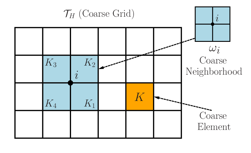
Multiscale model reduction methods aim at replacing the fine-scale mesh with a coarse-scale mesh when solving Problem (2.3) numerically, which, meanwhile, maintains a certain accuracy. To describe it, we need a few notations. The vertices of are denoted by , with being the total number of coarse nodes. The coarse neighborhood associated with the node is denoted by
| (2.4) |
We refer to Figure 1 for an illustration of neighborhoods and elements subordinated to the coarse discretization . Throughout, we use to denote a coarse neighborhood. Furthermore, Let (or ) be the collection of all edges in (or ) and let (or ) be the restriction of on (or on ).
Next, the multiscale ansatz space is constructed that are locally supported on certain coarse neighborhood . Then the multiscale-L1-scheme aims at seeking for , s.t.,
| (2.5) |
Here, denotes the multiscale space spanned by these multiscale basis functions and is a projection operator from to .
The construction of will be presented in Section 3. Note that we need a very tiny fine-scale time step size to guarantee a reasonable approximation property of to for due to, e.g., the singularity of the solution at when the source term fails to belong to certain smooth functional space. Consequently, the computational complexity and the storage requirement of the multiscale-L1-scheme (2.5) can be still extremely expensive. For this reason, we introduce in Section 2.3 the parareal algorithm to significantly improve its efficiency.
2.3 Parareal algorithm
The main goal of the parareal algorithm is to obtain a high-order approximation of the solution at the coarse time step for iteratively under the coarse time stepping scheme, which is corrected by parallel local fine time stepping scheme over each coarse subinterval. To demonstrate this algorithm, we need to introduce the one-step coarse propagator and fine propagator
for given initial data over the coarse interval . The outcome of these propagators is an approximation to for .
We present in Algorithm 1 the main ingredient of this method, which includes a parallel computation of the local jumps in Step 6 and the sequential propagation of the local jumps in Step 7. One can observe from [33, Theorem 2.1] that the solution operator to problem (1.1) is not a semigroup. Consequently, the fine propagator defined by the L1 scheme (2.2) requires all the information from the previous time steps. This results in a huge computational and storage cost. To reduce this cost, we will on the one hand, decrease the number of terms in the history part by means of approximation by exponential sums. One the other hand, the length of each term will be reduced by multiscale approximation.
The goal of this paper is to design an efficient numerical algorithm to approximate such that it can be solved on the coarse spatial mesh , without resolving the microscale information in the coefficient using a rather coarse time step that can be computational inexpensive. In the meanwhile, the storage cost can be reduced hugely. This is achieved by a combination of the multsicale method and parareal algorithm as proposed in [24] for parabolic problems with heterogeneous coefficients. Compared with parabolic problems, the main difficulty encountered here is that the solution operator of the time fractional diffusion problem is not a semigroup. This will be overcome in Section 4 by a new approximation by exponential sums.
3 Multiscale ansatz space
This section is concerned with the construction of the multiscale space by means of the Wavelet-based Edge Multiscale Finite Element Methods (WEMsFEMs) [15, 16, 23]. The main idea is to use wavelets as the boundary data to construct local multiscale basis functions on each coarse neighborhood . Then the multiscale ansatz space is constructed by multiplying these local multiscale basis functions with the partition of unity functions defined over the coarse patches .
Let be the partition of unity functions, which are the standard multiscale basis functions on each coarse element defined by
| (3.1) | ||||||
Here, is affine over with for all . Recall that are the set of coarse nodes on .
The construction of the multiscale test space is presented in Algorithm 2. Given the level parameter , and the type of wavelets on each edge of the coarse neighborhood , one can obtain the local multiscale space on by solving local problems in parallel in Step 2. One local multiscale basis function that is vanishing over is calculated in parallel. In Step 4, we can use these local multiscale space to build the global multiscale space by multiplying the partition of unity functions .
To analyze this algorithm, we define the weighted coefficient:
| (3.2) |
Furthermore, let be defined by
| (3.3) |
Next, we recap a few results on the approximation properties of the multiscale ansatz space which play a key role in the later convergence analysis (Section 6.1). The following assumption on the coefficient implies that is piecewise smooth.
Assumption 3.1 (Structure of and ).
Let be a domain with a boundary , and be pairwise disjoint strictly convex open subsets, each with a boundary , and denote . Let the permeability coefficient be piecewise regular function defined by
| (3.4) |
Here with for . Denote and . Furthermore, we assume the diameter of is 1.
Assumption 3.1, first proposed in [23] then further utilized in [15], is needed to make the constant appearing in the approximation properties independent of the possible contrast in the coefficient .
In the following, we define the -orthogonal projection onto the local multiscale space up to level by satisfying
| (3.5) |
Here, we denote for as the hierarchical bases defined on the four edges of of level and the local operator is defined as in Algorithm 2.
Let be the projection onto the multiscale space given by
| (3.6) |
Let be the elliptic operator defined on , and let its discrete operator be
Then the inverse operator exists, which is self-adjoint, positive semi-definite on , and positive definite on . Further, let be the Riesz operator associated to in the multiscale space , i.e.,
then the following relation holds
4 Model reduction in the history part
Recall that the time fractional operator can be split into a summation of the local component and the history component
| (4.1) |
We will approximate the local component by the L1 scheme and the history component by a new exponential sums inspired by sinc approximation [7, 34] in Section 4.1. Based upon this, a new local time integrator is presented in Section 4.2 that can handle long time simulation more efficiently.
4.1 Approximation by exponential sums
In order to deal with long time situation, we will construct a new approximation by exponential sums inspired by [7], which is essentially based upon Sinc quadrature to analytic, improperly integrable functions in , see [34]. Let be an analytic, improperly integrable functions defined on and let be the step size and , then we obtain by integration after Sinc interpolation to the following quadrature formula
Here, the second estimate is a direct truncation of the first estimate. The quadrature error can be estimated by the following theorem [34, Theorem 3.2.1].
Lemma 4.1.
Let be holomorphic in the strip with such that
Then taking , we obtain
Here, the hidden constant depends only on , and .
We will utilize Lemma 4.1 to derive a new exponential sums approximation to . To this end, we first rewrite it as an integral over of a analytic, improperly integrable function, which satisfies the conditions listed in Lemma 4.1.
Theorem 4.1 (Approximation by exponential sums for long time).
For all and , there holds
| (4.2) |
Given , as a function of is
| (4.3) |
The step size and the positive parameter are
| (4.4) |
Proof.
For any , by the definition of Gamma function, we obtain
Then taking integration by parts and a change of variables yields,
Here, as a function of parameterized by is defined in (4.3). In the following, we will verify that satisfies the conditions listed in Lemma 4.1 when .
Note that we attempt to use sum of exponentials to approximate the history component , and thus we demand an estimate (4.2) for instead. This, nevertheless, can be derived by a scaling argument.
Corollary 4.1.
For any and , there exist , s.t.,
| (4.6) |
with
Proof.
Next, making a change of variable by and using (4.3), lead to
Here,
Consequently, to guarantee
one only needs to choose sufficiently large, s.t.,
i.e.,
This completes the proof. ∎
In another word, a number of terms is required to have an approximation error below a tolerance . Note that this result is independent of the final time. Further, one can observe that and for all . Denote
| (4.7) |
then and .
Remark 4.1 ( Alternative approximation by exponential sums).
Another approximation by exponential sums are provided in [19, Theorem 2.5], For any , there exist , s.t.,
| (4.8) |
with
Note that this approximation is only suitable for cases with a final time of reasonable size due to the term in the total number of terms .
4.2 Local time integrators
We construct in this section local time integrators based upon the approximation by exponential sums developed in Corollary 4.1. The accuracy requirement of this exponential sums approximation is derived in (6.1), which implies that . The fine scale time step can be very tiny due to the possible singularity of the solution at the original due to, for example, insufficient regularity in the source term or the initial data . For this reason, we assume
| (4.9) |
for given tolerance throughout this paper.
Applying the summation of exponentials (Corollary 4.1) to the history component after taking integration by parts, we obtain
| (4.10) |
Here, the parameters for are defined by
which can be written as
This implies the following recurrence relation
Note that the integrals in the recurrence relation can be estimated by the L1 scheme, which yields
| (4.11) | ||||
with
| (4.12) |
Note also that the parameters for and rely only on and the parameter . Analogously, we can define with a coarse step size .
We establish an estimate of those parameters in the next lemma that provides a property of the history information.
Lemma 4.2.
Let for and be defined in (4.12) with or . Then it holds
Proof.
Remark 4.2 (Efficiency of the new time stepping scheme (4.10)).
can be defined similarly by replacing the fine time steps with the coarse time steps. One can observe from formulas (4.10) that each calculation of involves calculation and storage for . Note from (4.2) and (4.9) that and is independent of the final time as . Comparing with the L1 scheme (2.2), the new time stepping scheme is much more efficient.
For the sake of conciseness, we will rewrite the time integrator as
| (4.13) | ||||
Here, the propagation operator of the history information is
| (4.14) |
4.3 Multiscale-SOE-scheme
In this section, we formulate the numerical solution based on the time integrator (4.13) in the multiscale ansatz space . The multiscale-SOE-scheme aims to seeking for , satisfying
| (4.15) |
For the sake of the convergence analysis, we require a semidiscrete Galerkin scheme in the multiscale ansatz space , defined by seeking , satisfying
| (4.16) |
5 Wavelet-based Edge Multiscale Parareal Algorithm
We construct in this section the Wavelet-based Edge Multiscale Parareal (WEMP) Algorithm. To this end, we first recap a few terminologies commonly appeared in parareal algorithm. The one step coarse solver on the coarse subinterval is
| (5.1) |
which yields as a coarse approximation to , provided with an approximation of . Here, serves as the input parameter to calculate , which represents the memory effect from the previous time steps.
In matrix form, it reads
Here, we use the following notations,
where and are the mass matrix and stiffness matrix corresponding to the discretization of the elliptic operator in the finite element space , denotes the dimension of . for all , denotes a matrix with columns composed of the coefficients of multiscale basis functions in in the finite element space . Let be the dimension of the multiscale space . Note that is vector-valued function with components, and the length of each component is the dimension of the multiscale ansatz space .
The fine solver on the coarse subinterval is
| (5.2) |
which is defined in analogous to the one step coarse solver (5.1), but with a uniform discrete time step .
Analogously, we can define the semidiscrete Galerkin approximation in
| (5.3) |
Time stepping schemes with on top refers to the same scheme with a vanishing source term, for example, denotes the one step coarse solver with . and are defined analogously.
In the parareal algorithm 1, the cheap coarse time stepping scheme is sequentially utilized over the global time interval to provide a rough approximation to , while the expensive fine time stepping scheme is applied in each subinterval for in paralell to provide a more accurate solution. They do not agree with each other, and the discrepancy between them is denoted as the correction operator,
| (5.4) |
Here, denotes taking the first component.
In comparison with recently proposed parareal algorithm for time-fractional diffusion problems [38], our new proposed algorithm corrects only the solution . Its associated history component will be updated by (4.14) using the corrected solution . Extensive numerical tests shows that our proposed algorithm converges to the fine-scale solution within three iterations.
Next, we are ready to present our main algorithm, i.e., Algorithm 3. Its main objective is to obtain a good approximation to the exact solution of Problem (1.1) at the discrete coarse time step for , albeit that the time stepping scheme is built upon a coarse descretization. This relies on a parallel correction operator defined by (5.4).
We can solve (4.15) using the coarse-scale time stepping scheme as the initial guess for . Given the iteration parameter , we apply the local coarse solver (5.1) in Step 4 to obtain . Using the coarse solution as the initial condition, the fine solver (5.2) subsequently is used to calculate the fine solution in paralell on each local time subinterval . Then we calculate the discrepancy between the coarse solution and the fine solution in Step 6 on each discrete coarse time point for , and denote it as . Subsequently, this jump term is utilized in Step 7 to correct the coarse solution calculated by the global coarse solver (5.1). This process will be performed iteratively until certain tolerance on the jump terms is satisfied.
6 Error analysis
This section is concerned with the convergence analysis for the multiscale-SOE-scheme (4.15) and the WEMP Algorithm 3.
6.1 Error analysis for the multiscale-SOE-scheme (4.15)
To derive the error estimate for Problem (4.15), we start with a regularity property of the semidiscrete Galerkin approximation solution in Lemma 6.1 that is standard in the numerical analysis, see, e.g., [20]. We then show in Lemma 6.2 that the local time stepping scheme based on summation of exponentials is a small perturbation of the L1 scheme . Based upon this, we establish the stability estimate of Problem (4.15). Finally, the error estimate is presented in Theorem 6.1.
We begin with establishing a certain regularity result of the semidiscrete Galerkin approximation solution with respect to the temporal variable , which is similar to [20, Assumption 3.7].
Lemma 6.1.
Let be the solution to (4.16), then there holds
| . | |||||
Here, and throughout this paper, denotes a positive constant that is independent of , , and with varying value from context to context.
Next we present the truncation error estimate of our proposed time integrator :
Lemma 6.2.
Let be the solution to (4.16), then there holds
Proof.
An application of the triangle inequality implies
The first term can be estimated by [20, Lemma 3.9], and a direct calculation leads to the estimate of the second term. ∎
Lemma 6.3 (Stability of Problem (4.15).).
For any given positive parameter , let be sufficiently small, s.t.,
| (6.1) |
Then it holds
Moreover, there holds for any that
Proof.
On the one hand, we can derive by (4.1) and (4.10),
with
Together with (2.2), this yields
with
On the other hand, [20, Lemma 3.4] implies
which, combining with (6.1), yields
Then the desired result follows from an energy argument by mathematical induction analogous to the proof to [20, Theorem 3.5]. ∎
Note that the stability of Problem (4.15) using L2 time stepping scheme and summation of exponential approximation was derived in [39], which imposed a more restrictive constraint on than our proposed requirement (6.1).
Theorem 6.1 (Convergence rate of Problem (4.15).).
Assume that (6.1) holds. Let and with , then there holds
Proof.
The proof is analogous to [20, Theorems 3.10 and 3.11]. ∎
6.2 Convergence analysis for WEMP Algorithm 3
This section is concerned with the convergence of our main algorithm (Algorithm 3). We will first derive the approximation properties of the one step coarse time stepping scheme in the first component and the jump operator in Lemma 6.4. The convergence of Algorithm 3 is derived by the mathematical induction on the solution itself, based upon which we can derive the convergence rate of the history information using (4.14). This will lead to the inequality (6.15), and then the proof follows from [24, Theorem 4.1].
To start with, we first introduce a new norm to measure the effect of the history component.
Definition 6.1.
Let with each component . Then we define its associated history contribution by . This vector is measured by the following norm
We next prove the boundedness and Lipschitz continuity properties of the first component of the coarse solver and the jump operator in the multiscale space :
Lemma 6.4.
Let for with being the initial data, and let with and . Denote for that represents the history information at the previous iteration. Then for all , the following properties hold.
- 1.
The one step coarse solver is Lipschitz in . There holds
- 2.
The jump operator has the following approximation property. For any , it holds
(6.2)
Proof.
1. Let and let for , then it holds for all multiscale test function ,
Choosing leads to
Then an application of Young’s inequality implies
The a direct calculation proves the first assertion.
2. To prove the second assertion, let
To estimate , we only need to derive the estimate for and , separately.
Firstly, we introduce the following semidiscrete Galerkin approximation problem in the spatial domain : let satisfy
| (6.3) | ||||
Note that the error equation for derived from a fully discretization problem with L1 scheme in the temporal domain is
| (6.4) | ||||
with being the approximation error from L1 scheme,
which can be estimated by Lemma 6.2,
The stability estimate [20, Theorem 3.5] implies
Analogously, we can obtain the estimate for , which reads
Note that , then a combination of the two estimates above with the triangle inequality, shows the second assertion. ∎
Remark 6.1.
The key idea to prove the approximation property of the jump operator lies in the auxiliary problem (6.3), which is a time-fractional problem defined in the subdomain . Together with the history information on from the terms and , this results in a time-fraction problem on , with both and as its temporal discretization under time step size of and , respectively.
We present in the following a smoothing property of the SOE-scheme (4.13) that plays a crucial role in the convergence analysis with rough initial data. This property has been utilized without proof in [24, Assumption 4.1]. This property is proved by first establishing the global fully discretized scheme for , and then derive the global error equation between the multiscale SOE scheme (4.15) and Algorithm 3 to eliminate the source term .
Lemma 6.5 (Smoothing property of the SOE-scheme (4.13)).
Proof.
Note that Algorithm 3 is equivalent to seeking for , satisfying
| (6.6) |
Here, the local correction . Note that for all , it holds
Let , then it satisfies
| (6.7) |
with the source term being
Note that , Lemma 6.2 implies
By an application of Lemma 6.3 to the error equation (6.7), we obtain
Consequently, we obtain
We present in the next theorem the convergence rate of Algorithm 3 to Problems (1.1) in pointwise-in-time in -norm. To derive it, we first decompose the error from Algorithm 3 as a summation of the error from Problem (4.15) and the error from parareal algorithm. The former part is estimated by Theorem 6.1.
Theorem 6.2 (Error estimate of Algorithm 3 to Problem (1.1) in -norm).
Let Assumption 3.1 hold. Assume that the source term and initial data . Let be the level parameter. The coarse time step size and fine time step size are and . Assume that is sufficiently small, s.t.,
| (6.8) |
Let be the solution to Problem (1.1) and let be the solution from Algorithm 3 with iteration . Assume that the iteration number is not large. Then for any , it holds
| (6.9) | ||||
Proof.
We first split the error as the summation of and for with . Similarly, let , then it holds . Here, is the solution to Problem (4.15) and the error estimate is presented in Theorem 6.1.
We next estimate the error induced by parareal algorithm in the multiscale method, i.e., the second term . We will prove:
| (6.10) |
Obviously, the inequality (6.10) holds when . Assume that it holds for iteration for some . We will show that it holds for the next iteration . Before that, we first derive the error estimate for the history information. Let be a positive parameter, then Lemma 4.2 implies
| (6.11) | ||||
| (6.12) |
Here, is defined in (4.7) and we have used (6.8) in the last inequality.
Apply this inequality iteratively, we obtain
| (6.13) |
By (6.10), we derive
| (6.14) |
Next we estimate . We can obtain from Algorithm 3:
Consequently, an application of Lemma 6.4 and Lemma 6.5 leads to
for any . That is,
Let be a positive parameter, then together with the inequality (6.12), we obtain
Notice that
and
These, together with inequalities (6.10) and (6.14), lead to
Consequently, we derive
| (6.15) |
Repeat this recurrence relation, we obtain
where
The last inequality above holds because . Notice that we have proved in [24, Theorem 4.1] that is uniformly bounded with respect to when is small. Consequently, this proves the case for , and completes the proof. ∎
7 Numerical experiment
In this section, we perform a series of numerical experiments to demonstrate the performance of the proposed WEMP Algorithm. Let the spatial domain be . The coarse-scale and fine-scale mesh sizes are and . The coarse-scale and fine-scale time step sizes are and . For all the numerical tests, we take the level parameter . A larger can significantly reduce the spatial error. We take a smooth initial data,
The error is measured in -relative error and -relative error, defined by
where and denote the reference solution and its approximation at , respectively.
7.1 The influence of and
We study in this section the influence of and to the accuracy of (2.3) when we replace the L1 scheme with the summation of exponential approximation , i.e., we solve for for satisfying
Let , then (6.1) implies the minimum requirement of is .
7.1.1 Smooth source term
The first series of numerical tests are presented in Figures 2 and 3, with a smooth source data, different numbers of terms in the SOE approximation and different values of and . The source term is
One can observe from both cases that a more economic numerical scheme yields almost the same accuracy even with a much larger tolerance . For example, using a number of summations with , both -relative error and -relative error are below 0.15% for in Figure 3. The performance for a smaller is better as it is shown in Figure 2 that both -relative error and -relative error are below 0.0003% in this case.


7.1.2 Rough source term
The next series of numerical tests are presented in Figure 4, with a rough source term and different numbers of terms in the SOE approximation. The rough source term has jump along the temporal variable, defined by
Compared with Figure 3, the influence of rough source term is negligible. We observe similar behavior for varying . For the sake of conciseness, we only present the results for in Figure 4.


7.2 The performance of Algorithm 3
Next, we present the performance of Algorithm 3 with different , and iteration number . The convergence history is presented in Figure 5, Figure 6 and Figure 7. For all tests, Algorithm 3 converges within 3 iterations, this explains the fact that most lines in these figures overlap. We observe that the relative -error is less than in the 3 iteration. We can not reduce further this error due to the coarse scale mesh size . To reduce this error further, we need to decrease . Slightly more iteration numbers are needed for larger parameter .


7.3 The performance of Algorithm 3 for long time
We test our proposed algorithm for longer time in this section with . The parameters of and are determined by Lemma 6.3 and Corollary 4.1. Similar convergence behavior is observed as in the previous section, which is shown in Figure 8. For example, the -relative error is below 5% for and after 3 iteration. However, the performance for is slightly worse with -relative error below 10% after 3 iteration. In this case, the performance of multiscale-SOE-scheme has a slightly larger error as observed from Figure 8(c).


8 Conclusion
We propose in this paper a new efficient algorithm for time-fractional diffusion equations with heterogeneous coefficients. This algorithm is named as the Wavelet-based Edge Multiscale Parareal (WEMP) Algorithm, which can reduce computational cost and storage cost significantly. Moreover, it is suitable for long time simulation when multiple processors are available. We want to remark that the total number of terms in the exponential sums can be reduced hugely for a given accuracy requirement (4.2) if an adaptive representation instead of a uniform representation is utilized. Consequently, this will lead to a more efficient algorithm for more challenging applications, for example, for much longer time simulation.
References
- [1] R. Altmann, P. Henning, and D. Peterseim. Numerical homogenization beyond scale separation. Acta Numerica, 30:1–86, 2021.
- [2] G. Ariel, S. J. Kim, and R. Tsai. Parareal multiscale methods for highly oscillatory dynamical systems. SIAM J. Sci. Comput., 38(6):A3540–A3564, 2016.
- [3] G. Bal. On the convergence and the stability of the parareal algorithm to solve partial differential equations. In Domain decomposition methods in science and engineering, pages 425–432. Springer, 2005.
- [4] G. Bal and Y. Maday. A “parareal” time discretization for non-linear PDE’s with application to the pricing of an American put. In Recent developments in domain decomposition methods (Zürich, 2001), volume 23 of Lect. Notes Comput. Sci. Eng., pages 189–202. Springer, Berlin, 2002.
- [5] L. Berlyand and H. Owhadi. Flux norm approach to finite dimensional homogenization approximations with non-separated scales and high contrast. Arch. Ration. Mech. Anal., 198(2):677–721, 2010.
- [6] A. Blouza, L. Boudin, and S. M. Kaber. Parallel in time algorithms with reduction methods for solving chemical kinetics. Commun. Appl. Math. Comput. Sci., 5(2):241–263, 2010.
- [7] D. Braess and W. Hackbusch. Approximation of by exponential sums in . IMA journal of numerical analysis, 25(4):685–697, 2005.
- [8] A. Christlieb, C. Macdonald, and B. Ong. Parallel high-order integrators. SIAM J. Sci. Comput., 32(2):818–835, 2010.
- [9] W. E and B. Engquist. The heterogeneous multiscale methods. Commun. Math. Sci., 1(1):87–132, 2003.
- [10] Y. Efendiev, J. Galvis, and T. Hou. Generalized multiscale finite element methods. J. Comput. Phys., 251:116–135, 2013.
- [11] R. Falgout, S. Friedhoff, T. Kolev, S. MacLachlan, and J. Schroder. Parallel time integration with multigrid. SIAM J. Sci. Comput., 36(6):C635–C661, 2014.
- [12] C. Farhat and M. Chandesris. Time-decomposed parallel time-integrators: theory and feasibility studies for fluid, structure, and fluid-structure applications. Internat. J. Numer. Methods Engrg., 58(9):1397–1434, 2003.
- [13] C. Farhat, J. Cortial, C. Dastillung, and H. Bavestrello. Time-parallel implicit integrators for the near-real-time prediction of linear structural dynamic responses. Internat. J. Numer. Methods Engrg., 67(5):697–724, 2006.
- [14] P. Fischer, F. Hecht, and Y. Maday. A parareal in time semi-implicit approximation of the Navier-Stokes equations. In Domain decomposition methods in science and engineering, volume 40 of Lect. Notes Comput. Sci. Eng., pages 433–440. Springer, Berlin, 2005.
- [15] S. Fu, E. Chung, and G. Li. Edge multiscale methods for elliptic problems with heterogeneous coefficients. J. Comput. Phys, 369(1):228–242, 2019.
- [16] S. Fu, G. Li, R. Craster, and S. Guenneau. Wavelet-based edge multiscale finite element method for helmholtz problems in perforated domains. To appear in Multiscale Model. Simul., 2021.
- [17] T. Hou and X.-H. Wu. A multiscale finite element method for elliptic problems in composite materials and porous media. J. Comput. Phys., 134(1):169–189, 1997.
- [18] T. Hughes, G. Feijóo, L. Mazzei, and J.-B. Quincy. The variational multiscale method—a paradigm for computational mechanics. Comput. Methods Appl. Mech. Engrg., 166(1-2):3–24, 1998.
- [19] S. Jiang, J. Zhang, Q. Zhang, and Z. Zhang. Fast evaluation of the caputo fractional derivative and its applications to fractional diffusion equations. Communications in Computational Physics, 21(3):650–678, 2017.
- [20] B. Jin and Z. Zhou. An analysis of Galerkin proper orthogonal decomposition for subdiffusion. ESAIM Math. Model. Numer. Anal., 51(1):89–113, 2017.
- [21] A. Kilbas, H. Srivastava, and J. Trujillo. Theory and Applications of Fractional Differential Equations, volume 204 of North-Holland Mathematics Studies. Elsevier Science B.V., Amsterdam, 2006.
- [22] F. Legoll, T. Lelièvre, and G. Samaey. A micro-macro parareal algorithm: application to singularly perturbed ordinary differential equations. SIAM J. Sci. Comput., 35(4):A1951–A1986, 2013.
- [23] G. Li. On the convergence rates of gmsfems for heterogeneous elliptic problems without oversampling techniques. Multiscale Model. Simul, 17(2):593–619, 2019.
- [24] G. Li and J. Hu. Wavelet-based edge multiscale parareal algorithm for parabolic equations with heterogeneous coefficients. J. Comput. Phys, 444, 2021.
- [25] G. Li, D. Peterseim, and M. Schedensack. Error analysis of a variational multiscale stabilization for convection-dominated diffusion equations in two dimensions. IMA J. Numer. Anal., 38(3):1229–1253, 2018.
- [26] Y. Lin and C. Xu. Finite difference/spectral approximations for the time-fractional diffusion equation. Journal of Computational Physics, 225(2):1533–1552, 2007.
- [27] J.-L. Lions, Y. Maday, and G. Turinici. Résolution d’EDP par un schéma en temps “pararéel”. C. R. Acad. Sci. Paris Sér. I Math., 332(7):661–668, 2001.
- [28] Y. Liu and J. Hu. Modified propagators of parareal in time algorithm and application to Princeton ocean model. Internat. J. Numer. Methods Fluids, 57(12):1793–1804, 2008.
- [29] Y. Maday. Parareal in time algorithm for kinetic systems based on model reduction. In High-dimensional partial differential equations in science and engineering, volume 41 of CRM Proc. Lecture Notes, pages 183–194. Amer. Math. Soc., Providence, RI, 2007.
- [30] Y. Maday, J. Salomon, and G. Turinici. Monotonic parareal control for quantum systems. SIAM J. Numer. Anal., 45(6):2468–2482, 2007.
- [31] A. Målqvist and D. Peterseim. Localization of elliptic multiscale problems. Math. Comp., 83(290):2583–2603, 2014.
- [32] I. Podlubny. Fractional Differential Equations, volume 198 of Mathematics in Science and Engineering. Academic Press, Inc., San Diego, CA, 1999. An introduction to fractional derivatives, fractional differential equations, to methods of their solution and some of their applications.
- [33] K. Sakamoto and M. Yamamoto. Initial value/boundary value problems for fractional diffusion-wave equations and applications to some inverse problems. J. Math. Anal. Appl., 382(1):426–447, 2011.
- [34] F. Stenger. Numerical methods based on sinc and analytic functions, volume 20 of Springer Series in Computational Mathematics. Springer-Verlag, New York, 1993.
- [35] T. Strouboulis, I. Babuška, and K. Copps. The design and analysis of the generalized finite element method. Comput. Methods Appl. Mech. Engrg., 181:43–69, 2000.
- [36] Z. Sun and X. Wu. A fully discrete difference scheme for a diffusion-wave system. Applied Numerical Mathematics, 56(2):193–209, 2006.
- [37] V. Thomée. Galerkin finite element methods for parabolic problems, volume 1054. Springer, 2006.
- [38] S.-L. Wu and T. Zhou. Parareal algorithms with local time-integrators for time fractional differential equations. Journal of Computational Physics, 358:135–149, 2018.
- [39] H. Zhu and C. Xu. A fast high order method for the time-fractional diffusion equation. SIAM Journal on Numerical Analysis, 57(6):2829–2849, 2019.