Luke Duttweiler, Sally W. Thurston, Anthony Almudevar
Testing Sparsity Assumptions in Bayesian Networks
Abstract
Bayesian network (BN) structure discovery algorithms typically either make assumptions about the sparsity of the true underlying network, or are limited by computational constraints to networks with a small number of variables. While these sparsity assumptions can take various forms, frequently the assumptions focus on an upper bound for the maximum in-degree of the underlying graph . Theorem 2 in Duttweiler et al. 2023 demonstrates that the largest eigenvalue of the normalized inverse covariance matrix () of a linear BN is a lower bound for . Building on this result, this paper provides the asymptotic properties of, and a debiasing procedure for, the sample eigenvalues of , leading to a hypothesis test that may be used to determine if the BN has max in-degree greater than 1. A linear BN structure discovery workflow is suggested in which the investigator uses this hypothesis test to aid in selecting an appropriate structure discovery algorithm. The hypothesis test performance is evaluated through simulations and the workflow is demonstrated on data from a human psoriasis study.
keywords
Bayesian networks, structure discovery, eigenvalue bound, sparsity assumptions, hypothesis test, eigenvalue inference1 Introduction
A Bayesian Network (BN) is a type of probabilistic graphical model built on a directed acyclic graph (DAG), which may be used to represent conditional independence or causal relationships among variables. A central focus of much of the research involving BNs is the process of structure discovery.
Bayesian Network structure discovery focuses on taking a data sample of variables, which are then treated as vertices in a DAG, and learning which edges exist between what vertices. Many algorithms for structure discovery exist, falling under the general categories of constraint-based and score-based algorithms. Some notable algorithms are the Grow-Shrink and PC-stable constraint-based algorithms of Margaritis 2003 and Colombo et al. 2014 respectively, and the score-based order-MCMC algorithm of Friedman and Koller 2003.
While structure discovery algorithms approach the problem in vastly different ways, they all make complexity-limiting assumptions about the underlying network, are limited to networks with a fairly low variable count, suffer from high false discovery rates, or some combination of all three of these issues. These issues are all related to the fact that the number of possible DAGs on variables grows super-exponentially in , leading to important questions about the amount of information available for structure discovery in a dataset where the sample size is not substantially larger than .
With these issues in mind, in this paper we develop a novel hypothesis test based on the largest eigenvalue of a transformation of the covariance matrix, which may be used to evaluate the assumption that the largest in-degree of a BN is equal to one. This method is novel not only in that this particular test has not been previously known, but also in that, to the best of our knowledge, this is the first method for learning structural information about a BN from data which does not require the direct use of a structure discovery algorithm.
We envision the proposed test as a part of a BN structure discovery workflow, in which an investigator first uses our hypothesis test to learn about the complexity of the underlying network. With this knowledge they are then able to select a structure discovery algorithm with a better understanding of which algorithms are appropriate for the task at hand, and in general will have more informed high-level knowledge of the type of network with which they are working.
Section 2 provides background and definitions for linear Bayesian Networks and DAGs, structure discovery, and some matrix algebra that may not be familiar to all readers. Section 3 presents the main theoretical results including giving an overview of the necessary estimation and inference needed for the hypothesis test. Section 4 details a simulation study of the method. Section 5 provides an example of the method’s use on real data. Section 6 gives a short discussion on this work along with possible future directions of research.
Appendix A provides technical details necessary for the estimation and inference on the eigenvalues needed in the hypothesis test. This section includes detailed results for minor advances in eigenvalue shrinkage-estimation, bias-correction, and inference. Appendix B discusses simulations focused on the eigenvalue estimation and inference results of Appendix A.
2 Background
In this section we provide definitions and background for linear BNs, structure discovery, and matrix algebra.
2.1 Linear Bayesian Networks
Definition 1.
We define a graph by , where is a set of vertices and is a set of edges between those vertices, and defines a weight function on the set of vertices such that
We assume for the remainder of this paper that for all .
For any graph we can define an adjacency matrix , which is indexed by the vertex set such that
Finally, if for all then we say that is undirected, whereas if for all then we say that is directed.
Definition 2.
We say that a path of length exists in from to if there is a set of distinct vertices such that , and for all A graph is called connected when for any vertex pair and there exists a path from to or from to .
When a path of any length exists from back to we call that path a cycle. An undirected graph with no cycles is called a tree if it is connected, and a forest if it is not connected.
A directed graph with no cycles is called a directed acyclic graph (DAG). Note that if is the adjacency matrix of a DAG, then we must have that is nilpotent (ie. there exists a positive integer such that ).
Definition 3.
Let be a DAG with weight function . Then for vertex we define the set of parents of as
and the set of children of as
We call the size of set the number of parents of or the in-degree of . We denote the maximum in-degree (or maximum parents) of a graph with , defined as
Then, following Frydenberg 1990 we define the Markov boundary of to be the set of parents of , children of and parents of the children of (not including ). In set notation,
Definition 4.
Let be a DAG with adjacency matrix . We define the moral graph of , denoted , as an undirected graph with adjacency matrix for which
Note that, as shown in Duttweiler et al. 2023, if and only if is a tree (or a forest).
Definition 5.
Let be a DAG on vertices with weight function and adjacency matrix . Then, for , let be a random vector indexed by . If we can write
where is a vector of independently distributed error terms with and we say that is a linear Bayesian Network (linear BN) with respect to . Note that this is equivalent to the definition of a linear structural equation model given in Loh and Bühlmann 2014, and that without loss of generality we assume is centered on 0.
In order to match standard statistical notation we denote
When the vertices in are ordered topologically such that for all then
Thus, a linear BN is a particular case of a Bayesian Network as defined in Pearl 2009.
There are several matrices related to a linear Bayesian Network that we will be using repeatedly throughout this paper. Below we provide their definitions.
Definition 6.
Let be a dimensional linear Bayesian Network with adjacency matrix and error terms . Let . Then, observe that , and therefore the covariance matrix of is defined and denoted as the matrix
We denote the inverse covariance matrix of by , and the diagonal matrix with the diagonal entries of and zeros everywhere else we denote as Then we denote the normalized inverse covariance matrix of by and the eigenvalues of by
Now, let be independent samples of . Then, we denote the sample covariance matrix by
the sample inverse covariance matrix by denote the diagonal of with and the sample normalized inverse covariance matrix with Then we denote the eigenvalues of with
2.2 Structure Discovery and Assumptions
Let be identical and independent samples of a linear BN with DAG , adjacency matrix , and moral graph . BN structure discovery is the process in which an investigator uses the samples to attempt to learn the true underlying graph , or equivalently, the true adjacency matrix .
While there are a significant number of available structure discovery algorithms, bringing a variety of different approaches to this problem, a common theme among many is an assumption that requires the underlying graph to be sparse. In fact, as demonstrated in Chickering 1996 and Chickering et al. 2004, all structure discovery algorithms either make sparsity assumptions or are limited by computational constraints to problems with a small number of nodes. As examples, the PC-stable algorithm of Colombo et al. 2014, the Grow-Shrink algorithm of Margaritis 2003, and the order-MCMC algorithm of Friedman and Koller 2003 are all popular BN structure discovery methods that make sparsity assumptions, while the exact discovery method of Silander and Myllymaki 2012 makes no sparsity assumptions, but is only computationally feasible on graphs which have less than 33 vertices.
These sparsity assumptions take various forms depending on the algorithm, but frequently depend (at least partially) on the maximum in-degree of the graph , which we denote with . It should be clear then, that any information that can be learned about assumptions on is of interest in the structure discovery process. If it can be reasonably justified from data that for some constant , this can open the door for faster algorithms that operate in higher dimensions. Particularly relevant to this paper, if the assumption (or equivalently that is a tree or forest) can be reasonably justified, then the polynomial time algorithm presented in Chow and Liu 1968 will provide a very fast and asymptotically consistent estimate of .
The main results in this paper provide a novel hypothesis test that can test the assumption that ( is a tree or forest), giving investigators more information when selecting an algorithm for BN structure discovery. However, before we present the hypothesis test, we provide a few more important definitions.
2.3 Some Matrix Algebra
In this section we present definitions for some matrices and matrix operators that may not be familiar to all readers. Readers interested in a thorough discussion of these operators and matrices should see Magnus and Neudecker 2019.
We begin with definitions of the Kronecker product and the vec operator.
Definition 7.
Let and be an and matrix respectively. Then the Kronecker product of and is the matrix defined by
Definition 8.
Let be an matrix, and let be the th column of . Then is a vector defined by:
We now present two matrices that can be very useful when working with Kronecker products and vectorized matrices. For a more complete exploration of the uses of the commutation matrix and the diagonalization matrix again see Magnus and Neudecker 2019 or Neudecker and Wesselman 1990.
Definition 9.
The commutation matrix, denoted , is defined as
where is a matrix with a 1 in the th position and 0s everywhere else.
For the remainder of the paper we will only be using the commutation matrix . Therefore, we suppress the subscript notation and write Then, following from Neudecker and Wesselman 1990, if and are both matrices we have
Definition 10.
The diagonalization matrix, denoted , is defined as the matrix
Again, because we will only ever be using we suppress notation and write this as . For the interested reader, is referred to as the diagonalization matrix as
where is the diagonalized version of with zeros in each entry except for along the diagonal where the original entries of are left intact.
This lemma, from Magnus and Neudecker 2019 p. 441, gives this useful relationship between the Kronecker product and the operator.
Finally, we define a particular version of the Frobenius norm, following Ledoit and Wolf 2004.
Definition 11.
Let be a matrix. Then, denotes the scaled, squared Frobenius norm.
3 Main Results
We now present the hypothesis test that is the main result of this paper. The theory behind the test is presented in section 3.1 and an outline for estimation and inference on the test statistic are presented in sections 3.2 and 3.3 respectively.
This test should be used as an important part of the BN structure discovery workflow, to confirm or reject an investigator’s use of any algorithm that assumes . This use is demonstrated in Section 5.
3.1 The Hypothesis Test
The hypothesis test developed in this section is based on the largest eigenvalue of the normalized inverse covariance matrix . Theorem 1 provides the justification for the test and was proven in Duttweiler et al. 2023.
Theorem 1 (Duttweiler et al. 2023).
Let be a linear Bayesian Network with moral graph and normalized inverse-covariance matrix , and let be the largest eigenvalue of . Then if is a tree or forest,we must have
Thus, in order to determine if is a tree (or equivalently ) the above result immediately suggests a hypothesis test with null and alternative hypotheses,
Therefore, defining as an appropriate estimator of , and as its estimated variance, we calculate our test statistic as
As we will demonstrate below, we can then expect with a large enough sample size that and reject if , where is the th quantile of the distribution and is the pre-selected level of the test. The degrees of freedom value of is used here as our corrected estimator of is a function of all sample eigenvalues (as will be demonstrated below).
In the following sections we outline the estimation of , and then inference on , which includes estimating The results in the following two sections are proven and explored in more detail in Appendix A, which contains the technical details.
3.2 Estimating
The primary issue with estimating is the significant bias exhibited by the sample estimate when the true value is small. Figure 1 demonstrates this bias by showing a Monte Carlo mean value of as a function of the true value As can be clearly seen in the figure, when is large there is little sample bias even when the sample size is low, but when is small there is significant positive bias. This is of particular importance in our case as, in order to avoid an inflated Type I error rate, our estimate of must not have bias that increases the expected value to greater than 2 when
Many techniques have been developed to deal with a similar estimation bias presented in the eigenvalues of the covariance matrix. While most of these techniques rely on large-sample properties or Gaussian generative distributions, many share an appealing common property of including a bias correction term that disappears as the sample size grows. For example, with representing the th eigenvalue of , the estimator
was suggested in Anderson 1965 as a method of correcting the sample estimate , while the estimator
was developed by Stein (as recorded in Muirhead 1987) under the assumption that the sample covariance matrix follows a Wishart distribution. More recently, estimators for the eigenvalues of the covariance matrix that function well in a small-sample setting have appeared (for example, see Mestre 2008).
Of course, these estimators are all developed for the covariance matrix itself and thus cannot be directly carried over for . However, this reduction of bias when can be achieved by combining a Stein-type shrinkage estimator for with a second-order bias correction based on the estimator proposed in Anderson 1965. The specifics for this method are worked out in Appendix A, and simulation studies related to these estimators are provided in Appendix B, but we outline the approach below. Figure 2 is taken from the simulation studies in Appendix B; we will refer to it throughout this section.
We begin with the shrinkage estimation, discuss the second-order bias correction, and then provide the suggested estimator for .

3.2.1 Shrinkage Estimation
Shrinkage estimators for stabilizing estimates of the covariance matrix in high-dimensional situations have grown greatly in popularity since the introduction of a Stein-type shrinkage estimator based on an objective function using the Frobenius norm in Ledoit and Wolf 2004. Further developments of this type of shrinkage estimator continue to be popular due to their computational speed, invariance to permutations, and invertability even when (see Touloumis 2015). Of particular interest to us, under particular generative models this family of estimators also does an excellent job of correcting the sample bias of eigenvalues described above.
Significant work has already been done in terms of developing this kind of shrinkage estimation targeted toward the inverse covariance matrix (see Nguyen et al. 2022 and Bodnar et al. 2016), so here we will simply develop a shrinkage estimator for the normalized inverse covariance matrix Additionally, we will focus only on the situation where as this aligns with the scope of the rest of the paper.
Here we present a Stein-type shrinkage estimator for based on a similar estimator that was proposed for the covariance matrix in Ledoit and Wolf 2004. As we will show, this estimator immediately provides a shrinkage estimator of .
The development required for the following Theorem is given in Section A.2.
Theorem 2.
Let be a random vector with finite moments up to the fourth order, and invertible covariance matrix . Then let be the normalized inverse covariance matrix of . Now, let be defined by
where is the usual sample estimate of and is the identity matrix. Then, the value which minimizes the quantity is given by
where is the covariance matrix of and .
Following the language in Ledoit and Wolf 2004 we note that as depends on the true value and true variance of , it is not a bona fide estimator. However, again following Ledoit and Wolf 2004, we use plug-in estimators for each component of , allowing the development of the bona fide estimator
where
An estimator of is provided below in Section A.1.4 (Corollary 1), immediately giving an estimator of . Additionally, it is important to note that, as shown in Section A.2.2, is an asymptotically consistent estimator of .
One very useful aspect of this shrinkage estimation is that the eigenvalues of follow the analytical formula
avoiding the need for additional computation, and ensuring that
As we can see, provides an estimator of which shrinks the sample estimate towards 1. However, as demonstrated in Figure 2, still has a tendency to exhibit positive bias when the true maximum eigenvalue of is small (close to 2). Thus, we introduce a second-order bias correction which in conjunction with the shrinkage estimation can further reduce the problematic bias, particularly for small .
In order to make Figure 2, we generated data sets of dimension and sizes under 5 different generative models. For model the data was generated so that , where we chose so that the largest eigenvalue of was In each situation we generated data sets and calculated and from each.

3.2.2 Second-Order Bias Correction
Matrix perturbation theory has been applied in several different ways to improve estimates of the eigenvalues of the sample covariance matrix (see Anderson 1965, Sakai et al. 2000, and Fukunaga 2013). This section makes a small adjustment to the application of a well-known matrix perturbation result (see Saleem 2015) in order to adjust for sample bias in the eigenvalues of . Theorem 3 presents a result that may be leveraged to further reduce bias in our proposed estimator. The development of this result is given in Section A.3.
Theorem 3.
Let be a random vector with finite moments up to the fourth order, and invertible covariance matrix . Then, defining the unit eigenvectors of as we have
Using sample estimates as plug-in values to this equation, this does suggest a bias-corrected estimator of . Again noting that an expression for is given in Section A.1.4 (Corollary 1), we define this bias-corrected estimator by
While does have less bias than , as demonstrated in Figure 2, the bias correction does not correctly account for all of the positive bias. Therefore, as suggested above, we will combine shrinkage estimation and the second-order correction to develop our proposed estimator.
3.2.3 The Proposed Estimator
Now, observe from Theorem 3, given we have
Therefore, for the best estimation of for our suggested hypothesis test, we propose the estimator
noting that, as desired
As can be seen from Figure 2, is the only estimator which does not exhibit a positive bias for any of the generative models, regardless of sample size. In the current situation, where any positive bias when will result in an inflated Type I error rate, is clearly the best estimator of the set we have examined here.
Of course, Figure 2 also demonstrates that, at lower sample sizes, has a strong negative bias when the true value of is large. This will reduce the power of our hypothesis test at lower sample sizes, but as the bias disappears asymptotically, the power will increase as expected with sample size.
3.3 Inference on the Maximum Eigenvalue of
The asymptotic distributions of the eigenvalues of the sample covariance and correlation matrices have been well studied under various conditions (seeAnderson 1965, Konishi 1979, Van Praag and Wesselman 1989, Neudecker and Wesselman 1990, and Kollo and Neudecker 1993). While early development of this theory depended on a multivariate normal generative model, later iterations have discarded this assumption and operate under much more general conditions. Theorem 4 extends these asymptotic distributions to the eigenvalues of under the multivariate normal case as a specialization of a more general result found in Section A.1. The development and proof of Theorem 4 can be found in Section A.1.
Theorem 4.
Let be a random vector with non-singular and assume is non-singular. Let be the vector of eigenvalues of and be the vector of eigenvalues of . Then,
where
and
where is the matrix of orthonormal eigenvectors of and is a matrix such that where is the unit vector with a 1 in the position and 0s elsewhere.
The formula given by Theorem 4 suggests a plug-in estimator of as where and are defined in Section A.1.4 and with as the matrix of orthonormal eigenvectors of Then, from Theorem 4 we see that is asymptotically normal and we can estimate the variance of with
Now denote the bias correction term with
and observe that
and since, given and , is simply a rescaling of , we know that asymptotically
Of course, a more accurate inference on would not be conditional on or as these quantities are estimates of constants, not constants themselves. However, the simulation studies below demonstrate that treating these two values as constants in the calculation of variance does not adversely effect the suggested hypothesis test.
With all of these calculations complete we denote and reiterate from above that
again noting that the degrees of freedom is as is a function of all eigenvalues.
We now provide the results of several simulation studies designed to test our methods performance both when the assumptions are satisfied, and when they are not.
4 Simulation Studies
In order to examine the accuracy of our method we ran several simulations under 5 different generative models. The generative models were designed so that model fulfills all assumptions, models and violate the normal errors assumption to differing degrees, and models and violate the linearity assumption in different ways. All five models are are described here in detail.
Model is the most basic model, satisfying all of our assumptions. A BN from model is a linear Bayesian Network with edge weights sampled from a Gaussian distribution and sampling errors generated from a multivariate normal distribution. Thus for generated from model we have
where is a nilpotent matrix with non-zero elements generated from a Gaussian distribution and In general we require to be a diagonal matrix, but do not require that for some constant
A BN from model is still a linear Bayesian Network with edge weights sampled from a Gaussian distribution but violates the assumption that the sampling errors are generated from a multivariate normal distribution and instead assumes that all sampling errors are generated from a distribution with two degrees of freedom. That is, for each component of from model we have
where is the values of the parents of , gives the edge weights of the edges from the parents of to (sampled from a Gaussian distribution), and
A BN from model is identical to that of model but the sampling errors are generated from a distribution with one degree of freedom so that the errors do not have a finite mean. That is, for each component of from model we have
where
Model departs from the linearity assumption. A BN from model is created by sampling an adjacency matrix with Gaussian edge weights and then assigning each component of the vector a link function and random distribution from the exponential family. Essentially, data is generated from a BN in model as if each component is a generalized linear model (GLM) where the linear components of each GLM are determined by the adjacency matrix. Specifically, for each component of from model we have
where the weights are chosen as in models . For each BN from model the conditional distribution was randomly chosen from the set (Gaussian, Bernoulli, Poisson) with probability , and the appropriate canonical link function was used.
Model departs from the linearity assumption in a different way. A BN from model is created by sampling an adjacency matrix with Gaussian edge weights and with non-linear functions from each parent to each child. That is, for each component of from model , we have
where is a function randomly chosen from the set with equal probability, and
We evaluated the performance of the proposed hypothesis test through several different simulations presented in two subsections below. The first subsection presents the results of hypothesis tests run on data generated from all of the models listed above, with varying values of and varying sample sizes, to demonstrate how the method reacts when the assumptions are met and when the assumptions are violated in different ways. The second subsection presents a detailed power study where data is generated only from model (so all assumptions are met) and is steadily increased in order to gauge how departure from the null hypothesis will affect statistical power.
4.1 Basic Simulations
Each of the three tables in this subsection reports the results from one simulation, where the simulations differ by each allowing a different value of the maximum number of parents () in the data generating Bayesian Network. In Simulation 1 each BN that is generated has , in Simulation 2 each has and in Simulation 3 each BN has .
Each simulation was performed by creating 400 BNs, each with vertices, per generative model, where each BN in a generative model was generated following the process described above. Each BN was then used to generate one dataset of each of the sizes The proposed hypothesis was performed at a level of on each data set and the percentage of results which returned a ‘Reject’ result is reported in the tables.
| Generative Model | |||||
|---|---|---|---|---|---|
| 30 | .05 | .045 | 0 | .045 | .04 |
| 50 | .0525 | .0775 | .055 | .0225 | .0075 |
| 100 | .025 | .04 | .1025 | 0 | 0 |
| 500 | .03 | .0575 | .2125 | 0 | 0 |
Table 1 shows the results from Simulation 1, in which each BN has , implying that the moral graph of the network is a tree and therefore, that is true. Thus, the results in Table 1 give a Monte Carlo Type I error rate for our hypothesis test under each of the generative models.
When all assumptions are met (Model ) the Type I error rate stays near .05, as desired. Additionally, when the normal errors assumption is relaxed but the errors still have mean 0 (Model ), the Type I error rate behaves well. On the other hand, when the errors come from a Cauchy distribution and have no mean (Model ), the Type I error rate inflates with the sample size. This error inflation is demonstrated by the bolded values. The two non-linear models ( and ) seem to be overly conservative with the Type I error rate going to 0 as the sample size gets larger.
This simulation demonstrates our methods exceptional robustness to non-normal errors. The errors in Model come from a distribution with 2 degrees of freedom, which is very far from a normal distribution. Additionally, while the hypothesis test does fail when the errors come from a Cauchy distribution, any preliminary examination of data generated in this way would reveal extreme outliers, demonstrating a need for caution.
| Generative Model | |||||
|---|---|---|---|---|---|
| 30 | .0725 | .055 | .015 | .065 | .0375 |
| 50 | .285 | .2975 | .2375 | .0225 | .025 |
| 100 | .595 | .68 | .6575 | .0075 | .0075 |
| 500 | .995 | .9925 | .9775 | .0475 | .04 |
Table 2 presents the Simulation 2 results. In Simulation 2 for each BN and therefore is false. Thus, the values in Table 2 give the Monte Carlo power for the proposed hypothesis test under each model type. All models that satisfy the linearity assumption (Models , and ) have power that increases with sample size, as we would want. However, as shown in bold, the models that do not satisfy linearity ( and ) all stay under the level of the test, regardless of sample size.
| Generative Model | |||||
|---|---|---|---|---|---|
| 30 | .0975 | .075 | .025 | .0325 | .0525 |
| 50 | .39 | .475 | .505 | .055 | .0775 |
| 100 | .865 | .925 | .885 | .035 | .0475 |
| 500 | 1 | 1 | .98 | .2225 | .365 |
Table 3 presents the Simulation 3 results, that differ from Simulation 2 only in that now instead of 4. Again, all of the models which satisfy linearity behave as expected with increasing power as the sample size grows. Additionally, the models that violate linearity seem to maintain a power value similar to the level of the test, until the sample size gets large enough with . When this happens, as shown in bold, the power of the test does increase although very slowly.
These simulation results seem to suggest that the proposed hypothesis test operates very effectively under the stated assumptions. Additionally, as long as the generating model errors are somewhat constrained (have a finite mean), the hypothesis test works well even when the assumption of normality is violated. However, if the generative model is non-linear, the above results show that the proposed test is severely underpowered, although it does remain conservative.
4.2 Power Study Simulations
In order to evaluate the power of the hypothesis test more thoroughly, we performed a power study.
To simulate data we began with a single directed graph with vertices, and for which the moral graph was a tree, implying that was true. was also designed as a complete graph, meaning that every vertex but the founding vertex had one parent. Thus, the addition of any edge into would cause to violate .
We then created ten new directed graphs by, each time, randomly adding 6 edges into . Thus, for each , was a graph that was 6 edges away from satisfying Following this, we created ten new graphs , where for each , was created by randomly adding 6 edges onto . We continued this process until we had generated , leaving us with 100 directed graphs (excluding ) which all violate the null hypothesis.
This data-generation process was used in order to provide some understanding of ‘distance from ’, by measuring distance using the number of edges away rather than by maximum in-degree in the graph. Of course, as the number of edges in a graph increases, so will for the graph.
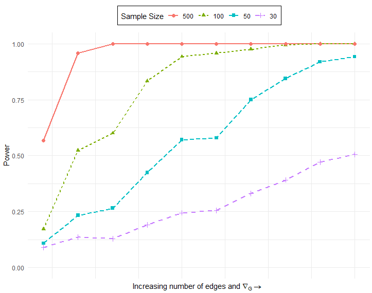
Then, for each of the 100 graphs, we generated random edge weights so that each could now function as a linear BN. Then, for each of the four sample sizes , we generated 300 samples from each BN. Our hypothesis test was evaluated on each data set and the results were averaged across graphs with an equal number of edges, giving a Monte Carlo estimate of the power of the test. These results are reported in Figure 3.
As would be expected, increasing the sample size improves the power of the test, even when the true graph isn’t far from satisfying the null hypothesis. Additionally, as we would hope, the power of the test is increased as the true graph gets farther away from satisfying , regardless of sample size.
5 Psoriasis Expression Networks
Psoriasis is a chronic disease in humans characterized by well-defined patches of skin which are scaly and inflamed. There is significant evidence, discussed in Baliwag et al. 2015 and Nickoloff et al. 2004, that these ‘lesions’ as they are referred to, are linked to the cytokines expressed in psoriasis skin. As such, there is interest in the gene expression network involving the genes that encode these cytokines.
While a standard approach to an analysis of this network may be to compare gene expressions using correlations or to fit an undirected or BN structure using data, the low sample sizes and high number of parameter estimations required for such a task can render these methods ineffective or misleading. Instead, as suggested by the methodology above, we propose here to learn important ‘global’ properties of this network in order to answer important questions with a lesser degree of uncertainty.
We demonstrate this global property-learning approach on a human psoriasis data set collected as a part of the ‘Improving Psoriasis Through Health and Well-Being’ clinical trial (NIH Project Number: R01AT005082). The data consists of two samples each from psoriasis patients where one sample contains gene expression levels from a psoriasis lesion and the other sample contains measurements of the same genes from a healthy patch of skin. An important and relevant question that may be asked about these two gene expression networks is ‘Are they the same?’ Of course, if the networks are in fact different, it would be best to quantify exactly how they differ, but this is difficult to accomplish with an acceptable degree of certainty at such a low sample size.
A permutation-based hypothesis test for the equality of two Bayesian Networks is proposed in Almudevar 2010. A slight modification of this test (for paired data) allows the user to test the equality of the lesion and non-lesion networks under the assumptions that the networks are Bayesian Networks and have a maximum in-degree of one. While the first of these assumptions must remain an assumption, we are now able to evaluate the validity of the second using the methodology described above.
We evaluated our hypothesis described above separately on both the lesion and non-lesion data to determine if the assumption that was reasonable for either underlying network. We failed to reject the null on both tests, with test statistic for the non-lesion sample and test statistic for the lesion sample, allowing us to assume for both networks.
One possible interpretation of this result is that, due to the low sample size, there simply isn’t enough information in the data to sustain a more complex estimate with any reasonable degree of certainty. The methods developed in this paper allow us to be more confident in assuming a simple model in order to learn what we can from the data without over-fitting.
5.1 Equal Networks?
We now test the equality of the lesion and non-lesion expression networks. The first network equality test proposed in Almudevar 2010 is a simple permutation test with iterations. For each iteration the samples are permuted into two groups of equal size, a tree is fit on each group using the algorithm introduced in Chow and Liu 1968, and a score is calculated using this spanning tree. For more details please see Almudevar 2010.
Using this hypothesis test (with a slight modification to ensure that the permutations were paired) with we calculated a p-value smaller than .001, indicating that the lesion and non-lesion gene expression networks are not identical, which may account for some of the up-regulated cytokines in psoriasis lesions.
In order to visualize this difference in networks we fit both networks separately using the minimum spanning tree algorithm from Chow and Liu 1968, which again assumes that . These networks are presented in Figure 4.
Additionally we present the networks fit using the TABU algorithm found in Russell 2010. We use the extended BIC of Foygel and Drton 2010 in this score-based algorithm in order to avoid a very dense network. Notice that for this algorithm we relax the assumption that .


6 Discussion and Future Work
The hypothesis test presented in this paper allows for investigation into a global property of a BN, namely the maximum number of parents, without needing to use an algorithm to fit a model. To our knowledge, this is the first method developed to learn global information about a network without needing to call a particular structure discovery algorithm. This global information can be used to provide justification for the use of certain algorithms and methods, while also helping to give a better overall picture of the underlying network structure.
This is all accomplished without the additional variability that comes from the many different choices made during the estimation of a BN, such as the choice of algorithm or information criterion. Additionally, despite the fact that our method requires an assumption of normality in theory, the simulations demonstrated a strong robustness to the violation of this assumption, except in extreme circumstances. Note however, that this test appears to have two important drawbacks.
First, because Theorem 1 does not give an if and only if statement, it is possible to have a BN with which also has a non-tree moral graph. This can lead to a situation where is true, but the moral graph is actually not a tree (). A second hypothesis test, which has the potential to overcome this problem, was suggested in Duttweiler et al. 2023. This second hypothesis test used all of the eigenvalues instead of just the largest, but the specifics lie beyond the scope of this paper.
Second, as demonstrated in the simulations, the test is severely under-powered in networks with non-linear relationships. While there are many networks of interest that can reasonably take on a linearity assumption (gene expression networks come to mind), there are plentiful examples of networks that cannot. We are hopeful that further research may provide methods to mitigate this problem.
In addition to further research into non-linearity, we hope to work toward estimation and inference on other global properties of Bayesian Networks, such as in-breeding and number of components, without needing to perform an entire structure discovery. Theorem 1 in Duttweiler et al. 2023 seems to lay a foundation for further methodology in this vein.
acknowledgments-disclosure-of-funding.
The authors would like to acknowledge the incredibly helpful comments and editing of Mr. Luke Rosamilia. Research reported in this publication was supported by the National Institute of Environmental Health Sciences of the National Institutes of Health (NIH) under award number T32ES007271. The content is solely the responsibility of the authors and does not necessarily represent the official views of the NIH. There is no competing interest.Appendix A
In the following section we discuss the more technical details required for estimation and inference on the largest eigenvalue of .
A.1 Asymptotic Distributions
We begin with a discussion of the asymptotic distributions of , and . We first overview necessary matrix derivatives, then apply these derivatives along with the delta method to develop asymptotically normal sample distributions.
A.1.1 Matrix Function Derivatives
Here we present three lemmas relating to the derivatives of vectorized matrix functions with respect to the vectorized matrix.
We begin with a derivative of the matrix function which inverts a non-singular matrix. This is a commonly known matrix derivative and thus the proof is omitted.
Lemma 2.
Let be a non-singular, , symmetric matrix. Then,
Next, we show the derivative of the matrix function that normalizes a square matrix. An excellent proof of this Lemma can be found in Neudecker and Wesselman 1990.
Finally, we present the derivative of the eigenvalues of a symmetric matrix with respect to the vectorized matrix. The full proof can be found in Kollo and Neudecker 1993.
Lemma 4 (Kollo and Neudecker 1993).
Let be a symmetric matrix with eigenvalues and associated orthonormal eigenvectors Let be the diagonal matrix with diagonal entries that are the eigenvalues and Finally, let be a function of the vector such that Then,
where is a matrix such that where is the unit vector with a 1 in the position and 0s elsewhere.
A.1.2 The Covariance Matrix
Before we can begin deriving the asymptotics for transformations of the covariance matrix, we must have an asymptotic distribution for the covariance matrix itself. The following result, establishing such a distribution under general conditions, was originally published in Neudecker and Wesselman 1990.
Lemma 5.
Let be a random vector with finite moments up to the fourth order. Then,
with
In the case that the data is generated from a multivariate normal distribution both Neudecker and Wesselman 1990 and Van Praag and Wesselman 1989 provide the following result.
Lemma 6 (Neudecker and Wesselman 1990 and Van Praag and Wesselman 1989).
Let be a random vector such that . Then,
A.1.3 The Inverse Covariance Matrix
Beginning with the inverse covariance matrix, we present the asymptotic distribution of the usual sample estimate under general conditions.
Proposition 1.
Let be a random vector with finite moments up to the fourth order and let be non-singular, and assume is also non-singular. Recall that we denote and . Then,
where
Proof:
Let be a function on vectorized, non-singular, symmetric matrices defined as
Now, by Lemma 2 we have that
Therefore, by the delta method and Lemma 5 we have that
A.1.4 The Normalized Inverse Covariance Matrix
Now that we have established the asymptotic distribution of the inverse covariance matrix we do the same with the normalized inverse covariance matrix .
Proposition 2.
Let be a random vector with finite moments up to the fourth order, with non-singular and assuming is non-singular. Then,
where
and
Proof:
Let be a function on vectorized, square symmetric matrices such that
where Then, observe that
Therefore, by Theorem 1 and the delta method, we must have
Then, since by Lemma 3 we have
then we must have
where
Therefore, our proof is complete.
Although it doesn’t simplify anything particularly well, by applying Lemma 6 we can obtain the following result in the normal situation.
Corollary 1.
Let be a random vector and let all other terms be as defined in Proposition 2. Then,
where
We denote , and note that an asymptotically unbiased estimator of may be derived by plugging in sample estimators of the various components found in Corollary 1. That is, with independent samples from , we suggest estimating with
where
and
The value in the denominator of the estimator is suggested in order to provide a more conservative estimate of than dividing by , but also to avoid the very restrictive requirement that , which would be required to divide by another justifiable denominator, . For more evidence on the usefulness of this choice, see the simulations in Appendix B.
A.1.5 The Eigenvalues of
Now we derive the asymptotically normal distribution of the eigenvalues of
Proposition 3.
Let be a random vector with finite moments up to the fourth order, with non-singular and assuming is non-singular. Let be the distinct eigenvalues of with Then,
where
and
where is the matrix of orthonormal eigenvectors of and is a matrix such that where is the unit vector with a 1 in the position and 0s elsewhere.
Proof:
Let be a function on vectorized, square symmetric matrices such that
where is the vector of eigenvalues of . Then, observe that
Therefore, by Proposition 2 and the delta method, we must have
Then, since by Lemma 4 we have
then we must have
Therefore, our proof is complete.
Finally, using Lemma 6 we get the (slight) simplification in the following result. This is presented above in Section 3.3.
Theorem 4.
Let be a random vector and let all other terms be as defined in Proposition 3. Then
where
A.2 Shrinkage Estimation
This section focuses on the technical details of the shrinkage estimation approach and is split into three subsections. In the first, we present the minimizer of a Frobenius norm-based objective function of and . In the second, we develop this function into a true estimator of using -consistent plug-in estimators of the different terms found in . Finally, in the third subsection, we explore the impact this has on the estimated eigenvalues.
A.2.1 Minimizing an Objective Function
Following Ledoit and Wolf 2004 we propose a Stein-type shrinkage estimator of the normalized inverse covariance matrix as
such that is minimized over .
It should be clear that the suggested form of is shrinking the sample matrix toward a target matrix, namely the identity matrix . Shrinkage estimation for the covariance and inverse-covariance matrices requires the researcher to spend a great deal of thought choosing a target matrix of the correct form. However, when dealing with the normalized inverse-covariance matrix no such choice is necessary as the diagonal of must be all ones by definition. Hence, we only need focus on shrinking toward the identity.
Under the assumptions that all expectations involved exist, and that (which is true asymptotically as shown in Proposition 2), this minimization problem has already been solved in Ledoit and Wolf 2004. We present a rewording of their minimization solution here, without proof.
This Lemma is easily verified through the proof in Ledoit and Wolf 2004 by substituting for and setting
Of course, since is a function of unobservable quantities we are unable to use this directly to estimate However, now following the development of similar theory (in a non-parametric setting) given in Touloumis 2015, we present as a function of several estimable quantities, which may be individually estimated, leading to a plug-in estimator of . This Theorem was presented above without proof in Section 3.2.
Theorem 2.
Let be a random vector and let be independent samples of . Define as the variance of . Consider the optimization problem determining
where . The solution is given by
Proof:
First, observe from Ledoit and Wolf 2004 (Lemma 2.1) that we have
Therefore from Lemma 7 we have
Then, since
and
then we must have that
Finally, observe that giving our result.
A.2.2 A Shrinkage Estimator for
We now discuss the estimation of , approaching the estimation through the plug-in estimation of each component of . As each is a function of the covariance matrix we also demonstrate that the sample estimates are consistent in , assuming that the data is generated from a normal distribution.
Recall from Proposition 2 that we have , where
and
Additionally, following from Lemma 6, we know that if then , where
Define the plug-in estimator where
and
We now have a simple, but important result.
Theorem 5.
Let be a random vector such that , and define all other terms as given in Proposition 2. Next, define as in Theorem 2, and
Then, is an -consistent estimator of .
Proof:
Recall that, as defined in Proposition 2, is an -consistent estimator for . Then, observe that we can easily define a function such that while Finally, observing that must be continuous we have by the continuous mapping theorem that is a consistent estimator for
Notice that in our plug-in estimator for the variance of we divide by . While with increasing and constant all three of these options are asymptotically equivalent, there is also an argument to be made for dividing by or The simulations in the Supplementary Material provide evidence for dividing by as we are assuming that but not necessarily , and as dividing by typically gives a more ‘conservative’ estimate for .
In any case, this estimator provides a method for an improved estimation of which exhibits several nice properties. Of particular interest to us, estimates of the eigenvalues provided through this shrinkage technique are very easy to compute, exhibit less variance, and demonstrate a significant decrease in small-sample bias in some cases. The next subsection explores the theoretical implications of this shrinkage on the eigenvalues.
A.2.3 Shrinking the Eigenvalues
Observe that once we have a shrinkage estimate of , call this estimate , we are immediately able to calculate the shrinkage eigenvalues, without computing an eigen-decomposition of .
Let be the th eigenvalue of . Then for the corresponding eigenvector we have
where
Thus, the vector of eigenvalues of is simply the vector of eigenvalues of shrunk toward the vector of ones with the exact same , and the orthonormal matrix of eigenvectors remains the same. This method of eigenvalue shrinkage possesses two important and intuitive properties (as opposed to the second-order bias correction described earlier), namely that and In addition, it is easy to see the reduction in variance from the shrinkage is
In some situations is less biased than , and in other situations the shrinkage increases bias. We explore this bias, along with other components of this paper, in the simulations below.
A.3 Second-Order Bias Correction
In the following section we present the technical details for the second-order bias correction method, which is a generalization of the second-order approach presented in Anderson 1965.
A.3.1 A Perturbation Theory Result
We begin the development of our general bias correction term with a well known result from matrix perturbation theory. Derivations of this result can be easily found (see Fukunaga 2013; Sakai et al. 2000; Saleem 2015) and so a proof is omitted here.
Lemma 8.
Let be a symmetric positive definite matrix with distinct eigenvalues , and corresponding unit eigenvectors . Let where is some symmetric random matrix with and , and let be the th eigenvalue of , with corresponding unit eigenvector . Then,
The difficulty with using this equation to develop a bias correction comes from calculating the expectation in the numerator of the sum. However, with a simple transformation involving Lemma 1, we can quickly apply this equation to reduce estimation bias.
A.3.2 A Plug-in Bias Adjustment
We now provide a simple result which expresses the difficult expectation given in Lemma 8 in terms of the variance of the perturbed matrix.
Lemma 9.
Let be a random matrix with and . Also, let be the th eigenvector of . Then for ,
Proof:
Observe,
Lemma 9 allows us to use the perturbation expression from Lemma 8 as a plug-in bias correction for any transformation of the covariance matrix for which we can estimate the variance. This idea is formalized in the following Theorem, which was presented above in Section 3.2 without proof.
Theorem 6.
Let be a random vector with finite moments up to the fourth order, and invertible covariance matrix . Then, defining the unit eigenvectors of as we have
Proof:
Observe that from Lemma 8, with , we must have that
which then by Lemma 9 gives
Appendix B
In this paper we have suggested multiple techniques for approaching the estimation of the eigenvalues of the normalized inverse covariance matrix , along with a Stein-type shrinkage estimator for itself. There are practical complications that come along with both of these problems that are most clearly seen through numerical simulations. Thus, in the following section we present simulations pertaining first to the estimation of the shrinkage parameter , and then to the estimation of the eigenvalues of .
B.1 The Shrinkage Parameter
Our first simulation goal is to examine the bias induced by estimating using In order to accomplish this we generated data sets of dimension and sizes under 4 different generative models. For model the data was generated so that , where we chose so that the true largest eigenvalue of was In each situation we generated data sets and calculated from each.
Recall that Theorem 5 gives
As mentioned above, it is reasonable to use or as in both situations we have a consistent estimator of and we have assumed . However, as can be seen in Figure 6 the choice of denominator has a significant impact on the bias in the estimation of
The left panel of Figure 6 shows the bias incurred when calculating using . As can be clearly seen, in situations when is larger (5.8 or 10.4 in our case), the small-sample bias is very small, and tends to slightly over-estimate . However, in situations where is smaller, then this particular estimate of severely under-estimates the true value in small samples.
This can be constrasted with the right panel of Figure 6, which shows the bias when using . In this case we see that when we have larger values of , tends to be somewhat over-estimated in small samples, while with smaller values of we see that is still under-estimated in small samples, but by a lesser margin.

These simulations lead us to recommend the use of in the denominator of , as in most situations it is more helpful to over-shrink rather than over-fit. However, if an investigator has reason to believe that in their situation is relatively large or desires to avoid over-shrinkage, then using in the denominator is also justified.
Either way, it is clearly seen that as the sample size increases the bias disappears, reinforcing the claim from Theorem 5 that is consistent.
B.2 The Eigenvalues of
We have presented several different estimators for the eigenvalues of . These are the sample, the second-order corrected, shrinkage and second-order shrinkage eigenvalues, denoted and respectively. In the following subsection we present simulations exploring the performance of these 4 different estimators at various sample sizes, and under various true models. We primarily focus on the estimation of the largest eigenvalue in these simulations, although we also present some results regarding the smallest eigenvalue.
As in the shrinkage simulations, we generated data sets of dimension and sizes under 5 different generative models. For model the data was generated so that , where we chose so that the largest eigenvalue of was In each situation we generated data sets and calculated and from each.
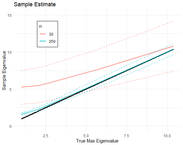

One of the interesting aspects of estimating the largest eigenvalue of is that the sampling bias generally decreases as the true maximum eigenvalue increases (holding both and constant). This is demonstrated in the left panel of Figure 7. As can be seen, the bias increases with smaller values of to the point that the true value lies outside the confidence interval, even at a higher sample size.
This problem remains for smaller values of even when using the shrinkage estimator . However, as shown in the right panel of Figure 7, using the second-order bias correction in combination with the shrinkage can be a successful technique for accurate inference on when the true value is smaller. Of course, the shrinkage bias prevents accurate inference on when the true value is larger, providing a trade off for investigators to consider.
Finally, we present bias results from our simulations which demonstrate the varied ways in which the different bias correction methods react under different generative models. Figure 8 shows the average Monte Carlo bias while estimating for each of the 4 methods presented in this paper, at multiple different sample sizes, and for the different generative models. As can be seen, for smaller true values of the shrinkage and second-order shrinkage methods work best, while for larger true values it is best to avoid shrinkage entirely.
As discussed above, we are interested in the use of in the hypothesis test with null and alternative hypotheses
The results shown in Figure 8 clearly indicate that under the null hypothesis (), the best estimation method is the second-order shrinkage approach as this is the only approach with no positive bias, which in the case of our hypothesis test, would artificially inflate the Type I error.
While estimating (the smallest eigenvalue), Figure 9 shows a significant amount of instability in the second-order correction method, as expected. Thus, we do not recommend using this technique unless the user is able to assume that the target eigenvalue is adequately separated from the others in the true model and in the sample. This assumption is generally most likely to be fulfilled in the largest eigenvalue, but can also be frequently fulfilled for the second largest or other higher rank eigenvalues. Typically however, the second-order bias correction method should not be used for the smallest or other lower rank eigenvalues as those tend to cluster together, at least in the sample.

References
- Almudevar (2010) Anthony Almudevar. A hypothesis test for equality of bayesian network models. EURASIP Journal on Bioinformatics and Systems Biology, 2010:1–11, 2010.
- Anderson (1965) George A Anderson. An asymptotic expansion for the distribution of the latent roots of the estimated covariance matrix. The Annals of Mathematical Statistics, 36(4):1153–1173, 1965.
- Baliwag et al. (2015) Jaymie Baliwag, Drew H Barnes, and Andrew Johnston. Cytokines in psoriasis. Cytokine, 73(2):342–350, 2015.
- Bodnar et al. (2016) Taras Bodnar, Arjun K Gupta, and Nestor Parolya. Direct shrinkage estimation of large dimensional precision matrix. Journal of Multivariate Analysis, 146:223–236, 2016.
- Chickering (1996) David Maxwell Chickering. Learning bayesian networks is np-complete. In Learning from data, pages 121–130. Springer, 1996.
- Chickering et al. (2004) Max Chickering, David Heckerman, and Chris Meek. Large-sample learning of bayesian networks is np-hard. Journal of Machine Learning Research, 5:1287–1330, 2004.
- Chow and Liu (1968) CKCN Chow and Cong Liu. Approximating discrete probability distributions with dependence trees. IEEE transactions on Information Theory, 14(3):462–467, 1968.
- Colombo et al. (2014) Diego Colombo, Marloes H Maathuis, et al. Order-independent constraint-based causal structure learning. J. Mach. Learn. Res., 15(1):3741–3782, 2014.
- Duttweiler et al. (2023) Luke Duttweiler, Sally W Thurston, and Anthony Almudevar. Spectral bayesian network theory. Linear Algebra and its Applications, 2023.
- Foygel and Drton (2010) Rina Foygel and Mathias Drton. Extended bayesian information criteria for gaussian graphical models. Advances in neural information processing systems, 23, 2010.
- Friedman and Koller (2003) Nir Friedman and Daphne Koller. Being bayesian about network structure. a bayesian approach to structure discovery in bayesian networks. Machine learning, 50(1):95–125, 2003.
- Frydenberg (1990) Morten Frydenberg. The chain graph markov property. Scandinavian Journal of Statistics, pages 333–353, 1990.
- Fukunaga (2013) Keinosuke Fukunaga. Introduction to statistical pattern recognition. Elsevier, 2013.
- Kollo and Neudecker (1993) Tônu Kollo and Heinz Neudecker. Asymptotics of eigenvalues and unit-length eigenvectors of sample variance and correlation matrices. Journal of Multivariate Analysis, 47(2):283–300, 1993.
- Konishi (1979) Sadanori Konishi. Asymptotic expansions for the distributions of statistics based on the sample correlation matrix in principal component analysis. Hiroshima Mathematical Journal, 9(3):647–700, 1979.
- Ledoit and Wolf (2004) Olivier Ledoit and Michael Wolf. A well-conditioned estimator for large-dimensional covariance matrices. Journal of Multivariate Analysis, 88(2):365–411, 2004.
- Loh and Bühlmann (2014) Po-Ling Loh and Peter Bühlmann. High-dimensional learning of linear causal networks via inverse covariance estimation. The Journal of Machine Learning Research, 15(1):3065–3105, 2014.
- Magnus and Neudecker (2019) Jan R Magnus and Heinz Neudecker. Matrix differential calculus with applications in statistics and econometrics. John Wiley & Sons, 2019.
- Margaritis (2003) Dimitris Margaritis. Learning bayesian network model structure from data. Technical report, Carnegie-Mellon Univ Pittsburgh Pa School of Computer Science, 2003.
- Mestre (2008) Xavier Mestre. Improved estimation of eigenvalues and eigenvectors of covariance matrices using their sample estimates. IEEE Transactions on Information Theory, 54(11):5113–5129, 2008.
- Muirhead (1987) Robb J Muirhead. Developments in eigenvalue estimation. Advances in Multivariate Statistical Analysis: Pillai Memorial Volume, pages 277–288, 1987.
- Neudecker and Wesselman (1990) Heinz Neudecker and Albertus Martinus Wesselman. The asymptotic variance matrix of the sample correlation matrix. Linear Algebra and its Applications, 127:589–599, 1990.
- Nguyen et al. (2022) Viet Anh Nguyen, Daniel Kuhn, and Peyman Mohajerin Esfahani. Distributionally robust inverse covariance estimation: The wasserstein shrinkage estimator. Operations research, 70(1):490–515, 2022.
- Nickoloff et al. (2004) Brian J Nickoloff, Frank O Nestle, et al. Recent insights into the immunopathogenesis of psoriasis provide new therapeutic opportunities. The Journal of clinical investigation, 113(12):1664–1675, 2004.
- Pearl (2009) Judea Pearl. Causality. Cambridge university press, 2009.
- Russell (2010) Stuart J Russell. Artificial intelligence a modern approach. Pearson Education, Inc., 2010.
- Sakai et al. (2000) Mitsuru Sakai, Masaaki Yoneda, Hiroyuki Hase, Hiroshi Maruyama, and Michiko Naoe. A quadratic discriminant function based on bias rectification of eigenvalues. Systems and Computers in Japan, 31(9):28–38, 2000.
- Saleem (2015) Mohammad Saleem. Perturbation theory. In Quantum Mechanics. IOP Publishing, 2015.
- Silander and Myllymaki (2012) Tomi Silander and Petri Myllymaki. A simple approach for finding the globally optimal bayesian network structure. arXiv preprint arXiv:1206.6875, 2012.
- Touloumis (2015) Anestis Touloumis. Nonparametric stein-type shrinkage covariance matrix estimators in high-dimensional settings. Computational Statistics & Data Analysis, 83:251–261, 2015.
- Van Praag and Wesselman (1989) Bernard MS Van Praag and Bertram M Wesselman. Elliptical multivariate analysis. Journal of Econometrics, 41(2):189–203, 1989.