Quasi-static magnetization dynamics in a compensated ferrimagnetic half-metal - Mn2RuxGa
Abstract
Exploring anisotropy and diverse magnetization dynamics in specimens with vanishing magnetic moments presents a significant challenge using traditional magnetometry, as the low resolution of existing techniques hinders the ability to obtain accurate results. In this study, we delve deeper into the examination of magnetic anisotropy and quasi-static magnetization dynamics in Mn2RuxGa (MRG) thin films, as an example of a compensated ferrimagnetic half-metal, by employing anomalous Hall effect measurements within a tetragonal crystal lattice system. Our research proposes an innovative approach to accurately determine the complete set of anisotropy constants of these MRG thin films. To achieve this, we perform anomalous Hall voltage curve fitting, using torque models under the macrospin approximation, which allow us to obtain out-of-plane anisotropy constants J m-3 ( T) and J m-3 ( T), along with a weaker in-plane anisotropy constant J m-3 ( T). By additionally employing first-order reversal curves (FORC) and classical Preisach hysteresis (hysterons) models, we are able to validate the efficacy of the macrospin model in capturing the magnetic behavior of MRG thin films. Furthermore, our investigation substantiates that the complex quasi-static magnetization dynamics of MRG thin films can be effectively modelled using a combination of hysteronic and torque models. This approach facilitates the exploration of both linear and non-linear quasi-static magnetization dynamics, in the presence of external magnetic field and/or current-induced effective fields, generated by the spin-orbit torque and spin transfer torque mechanisms. The detailed understanding of the quasi-static magnetization dynamics is a key prerequisite for the exploitation of in-phase and out-of-phase resonance modes in this material class, for high-bandwidth modulators/de-modulators, filters and oscillators for the high-GHz and low-THz frequency bands.
I Introduction
Spintronics-based devices have emerged as highly-promising candidates for next-generation telecommunication applications due to their potential for efficient control of magnetic moments via electrical methods, ultrafast operating speeds, and ultralow power dissipation Chappert et al. 2007. In the pursuit of these capabilities, antiferromagnetic (AFM) materials have demonstrated exceptional advantages over their ferromagnetic (FM) counterparts when incorporated into spintronic devices Jungwirth et al. 2016; Baltz et al. 2018. FM materials are limited by their large stray field interactions and slow switching speeds (on the order of nanoseconds) Khvalkovskiy et al. 2013; Demidov et al. 2012, which hampers their utility in memory and switching devices. In contrast, AFM materials project no stray fields and possess ultrafast spin dynamics (on the order of a few picoseconds to hundreds of picoseconds) Wadley et al. 2016, making them attractive for spintronics applications. However, the control and detection of magnetization in AFM materials remain challenging due to their zero magnetic moment and zero Fermi level spin polarization.
To address this technological gap, compensated ferrimagnetic half-metal (CFHM) Pickett 1998; Galanakis et al. 2007 materials have emerged as an excellent alternative to AFM materials. Similar to AFM materials, CFHMs also consist of two antiferromagnetically coupled spin sublattices, and their spin contribution can be conveniently tuned by adjusting the composition and/or temperature. Moreover, due to the presence of inequivalent spin sites, these sublattices contribute unequally at the Fermi level, resulting in a semiconducting band-gap in one of the spin channels and a zero band gap in the other Kurt et al. 2014. This disparity gives rise to a high spin polarization for the conduction electrons.
At the magnetic compensation point, CFHMs exhibit behaviour akin to AFM materials, demonstrating ultrafast magnetization dynamics. However, unlike AFM materials, the detection and manipulation of CFHM magnetization remain feasible due to the distinct responses of the two spin sublattices to electrical and optical excitation Siewierska et al. 2021; Banerjee et al. 2020; Teichert et al. 2021. These unique characteristics of CFHM pave the way for the development of novel spintronics devices with improved performance and functionality.
Following theoretical predictions Van Leuken and De Groot 1995, the first experimental observation of a CFHM thin film was achieved with the Mn2RuxGa (MRG) class of materials Kurt et al. 2014. MRG crystallises in the inverse-Heusler XA structure, space group , as depicted in figure 1. Within this structure, Mn occupies two distinct and non-equivalent sublattice sites: (Mn4a) and (Mn4c).
The Magnetic moments of and sublattices exhibit antiferromagnetic coupling, whereas moments located on identical sites display ferromagnetic coupling. Owing to the non-equivalent crystallographic surroundings, the magnetic moments of both sublattices display quite distinct temperature-dependent characteristics. The site-specific magnetic moment attributable to Mn4a possesses weaker temperature dependence in contrast to Mn4c sublattice moment Betto et al. 2015. As such, it is possible to attain an ideal magnetic compensation for MRG by modulating its composition and/or inducing crystal lattice distortion.
MRG displays pronounced -axis magnetic anisotropy due to the evanescence of magnetic moments, with an anisotropy field surpassing 14 T in proximity to the compensation point. Furthermore, the Fermi level of MRG is predominantly influenced by the electronic states originating from Mn situated at the position, subsequently dictating the transport phenomena via Mn4c electrons Fowley et al. 2018. Additionally, MRG displays half-metallic properties, as corroborated by Density Functional Theory (DFT) calculations Žic et al. 2016 and Point Contact Andreev Reflection (PCAR) spectroscopy (spin polarization obtained as high as ) Kurt et al. 2014; Siewierska et al. 2021. The highly spin polarized carriers lead to a large anomalous Hall effect (AHE) Fowley et al. 2018 and magneto-optic Kerr effect (MOKE) Siewierska et al. 2018; Banerjee et al. 2020 even at the perfect magnetic compensation. Therefore, the distinctive amalgamation of a vanishing net magnetic moment, high spin polarization at the Fermi level, and high magnetic anisotropy designates MRG as a promising contender material for active layers of next-generation spintronics devices.
By employing MRG as an active layer in the spin-oscillator, sub-THz chip-to-chip communication could be achieved, as its spin excitations were found to reside in the necessary terahertz gap Troncoso et al. 2019. The sub-THz excitations of MRG were ascribed to its low magnetic moment, high uniaxial anisotropy field, and low Gilbert damping Troncoso et al. 2019; Awari et al. 2016. In addition, the tunability of the anisotropy constant and the moment in MRG afford the flexibility to modify the resonance frequencies of oscillators constructed with MRG. Consequently, determining the anisotropy constants of MRG thin-films is a crucial preliminary step in examining their magnetization dynamics under the influence of external stimuli.
Investigating anisotropy and other magnetization dynamics in a sample with a negligible magnetic moment is unattainable using conventional magnetometry techniques (VSM, SQUID, etc.) due to insufficient resolution and sensitivity. Furthermore, for a sample with an extremely small magnetic moment (), both the anisotropy field () and coercive field () typically diverge, rendering the measurement of magnetic anisotropy unfeasible with exceedingly large magnetic fields ( T) Fowley et al. 2018. Generally, anisotropy is assessed by applying an external magnetic field at a specific angle () to the magnetic easy axis and monitoring the corresponding changes in physical properties such as magnetization Fan et al. 2007; Endo et al. 2000; Jagla 2005, anomalous Hall effect (AHE) Okamoto 1983; Sato et al. 2011, and magneto-optical properties Suran et al. 1999; Berling et al. 2006; Cowburn et al. 1997. The acquired data are then conventionally fitted using the torque balance method, which ultimately yields the anisotropy constants of the specimen.
In this study, an analysis of magnetic anisotropy and quasi-static magnetization dynamics in MRG thin-films, featuring a tetragonal crystal structure, is conducted through electrical transport measurement techniques (AHE). MRG demonstrates a pronounced uniaxial out-of-plane anisotropy and a small yet significant four-fold in-plane anisotropy, which originates from substrate-induced compressive strain. MRG exhibits a substantial anomalous Hall effect, alongside a high magnetic anisotropy field and high Fermi-level spin polarization, a combination that enables direct probing of the anisotropy in MRG thin-films via electrical means. The manipulation of the magnetization vector () of MRG within a 3D space, under the influence of a magnetic field, enables the examination of various anisotropy constants of the film. To characterize the equilibrium or dynamic response of the magnetization vector within an applied or induced effective field, accounting for the magnetic anisotropy of the sample is crucial. Generally, the equation of motion for magnetization is spatially non-uniform (described by a micromagnetic model) or, in a much simpler case, spatially uniform (explained by a macrospin model). This study employs the anomalous Hall effect to examine magnetic anisotropy in MRG, within the macrospin model framework, in combination with a distribution of hysterons, with finite magnetic viscosity and negligible interaction field.
This paper commences with a discussion of the sample preparation and characterization techniques employed in this study (section II). Subsequently, section III.1 introduces the modeling of hysteresis in MRG under a classical Preisach model and the first-order reversal curves (FORC) method, wherein the validity of the macrospin model for MRG is established within the FORC and Preisach frameworks. A comprehensive torque model for evaluating the anisotropy constants of MRG using AHE is explored in section III.2. Moreover, section III.3 examines various intricate static and quasi-static magnetization dynamics of MRG through a ’combined’ Preisach and torque model. Lastly, conclusions are drawn in section IV.
II Experimental details
Epitaxial thin films of Mn2RuxGa were fabricated using a DC magnetron sputtering system on a MgO (001) substrate. The films were co-sputtered in an inert environment (argon gas) from and Ru targets onto the substrate, which was maintained at . Additional details regarding film growth and characterization can be found in a separate publication Siewierska et al. 2021. This study focuses on the stoichiometry and a film thickness of approximately . The compensation temperature () of this sample is considerably higher than room temperature, at , as determined by SQUID® magnetometry measurements. To prevent oxidation, the films were in-situ capped with approximately of amorphous AlOx, deposited at room temperature. The substrate-induced compressive strain () facilitated the out-of-plane magneto-crystalline anisotropy in the film. To investigate the transport properties, the films were patterned into micron-sized ( ) Hall bars, using UV photolithography and Ar-ion milling. A subsequent round of lithography and metal deposition was performed to establish the contact pads and to minimize the series resistance contribution of the corresponding contacts, consisting of Ti ()/Au ().
The electronic transport properties were measured using the Quantum Design Physical Property Measurement System (PPMS®) in the temperature range of and magnetic field strengths of . The longitudinal and transverse voltages were measured by applying a lock-in demodulation technique at the first harmonic with low excitation frequency, typically , which was significantly smaller than the resonance frequencies of MRG. To determine the angular dependence of the resistivity, measurements were taken on a rotating platform within the PPMS, with an angular resolution of 0.01 deg. Additionally, First Order Reversal Curves (FORC) were measured using a field resolution of at room temperature in a GMW® electromagnet.
III Results and Discussion
III.1 Hysteresis model
This section discussess the approach taken to model the switching of the magnetization (magnetic hysteresis) using the classical Preisach (hysterons) model. Hysteresis modeling has been an active area of research for decades, owing to both physical and mathematical interest. The magnetic hysteresis of ferromagnetic materials is the most famous example of hysteresis. It is widely accepted that the multiplicity of metastable states is the origin of hysteresis. Consequently, a micromagnetic model must be considered for hysteresis modeling. In 1935, Preisach Preisach 1935 proposed a classical micromagnetic mathematical approach to describe the hysteretic effect. The Preisach model (PM) employs a large number of interacting magnetic entities (referred to as hysterons), each of which has a rectangular hysteresis loop (figure 2a). These hysterons are characterized by the operator , where is an arbitrary input variable, such as an applied magnetic field. Hysteresis arises from the collective behavior of numerous hysterons, which switch fully at a discrete applied field. The value of relies on the applied field history. For instance, if the applied field starts from the saturation state (), initiates at . The value of transitions to when the applied field falls below the value , and returns to when the field value exceeds . Typically, the switching fields and are not identical.
The interaction field experienced by a hysteron is defined by , resulting in an asymmetric elementary hysteron. In contrast, a hysteron with no interaction is symmetric. The coercive field of a hysteron is defined as . In a realistic sample, the hysteresis property is a weighted sum of a large number of hysterons, as described in equation 1:
| (1) |
Here, the weighting factor represents the distribution of the switching fields and and is commonly referred to as the switching field distribution (SFD) or hysteron distribution (HD). Figure 2b illustrates a schematic representation of the Preisach model.
In the continuum limit, the discrete model is transformed into the following expression:
| (2) |
where, is an arbitrary variable (e.g., applied magnetic field) and is the resultant hysteresis output (e.g., magnetic moment, anomalous Hall voltage, etc.). The most challenging aspect of the Preisach model involves uniquely defining the distribution function . Nevertheless, for an assembly of weakly interacting hysterons, it is possible to assume that the distribution function follows a specific statistical distribution. Common choices include the Gaussian function Della Torre 1986; Kádár et al. 1989, Gauss-Lorentzian function Fuzi 2003, and Lognormal-Gaussian distribution function Henze and Rucker 2002, among others. However, this approach faces the issue of lacking justification for selecting one particular distribution over others Henze and Rucker 2002. An alternative method entails using a linear combination of a set of functions as a basis. The drawback of this approach is the requirement of a large set of basis functions and their coefficients to obtain a Preisach distribution with a relatively continuous output (y) Galinaitis et al. 2001, which rapidly strains computational capabilities, even for modern computers.
The first-order reversal curves (FORC) method offers an experimental technique for obtaining a unique Preisach distribution, as long as the sample of interest meets the necessary and sufficient Mayergoyz conditions Mayergoyz 1986. The FORC method is both easily achievable experimentally and highly reproducible, given that it begins by saturating the sample each time. It has been employed to examine various magnetic systems, such as permanent magnets Chiriac et al. 2007; Chen et al. 2014, geological samples Roberts et al. 2000; Muxworthy and Roberts 2007, nanowires Béron et al. 2006; Béron et al. 2008, and more. Moreover, FORC can differentiate between interacting and noninteracting single domain (SD), pseudo single-domain (PSD), and multi-domain (MD) systems Pike et al. 1999; Roberts et al. 2000. In fact, the FORC method can be extended to any system exhibiting hysteresis behavior, including ferroelectric samples Stancu et al. 2003; Ramírez et al. 2009. Additionally, FORC studies on certain magnetic systems can be complemented by AHE measurements, where electrical probing presents a decisive advantage over standard magnetic moment measurements Diao et al. 2012.
The FORC measurement using AHE commence by saturating the sample in a sufficiently high positive magnetic field. Subsequently, the field is decreased to a lower field value on the main hysteresis loop (MHL), referred to as the reversal field (), and the Hall resistance is measured by sweeping the applied field back to the saturation field. The resulting AHE resistance, , constitutes a minor curve within the MHL (figure 3a). This procedure is repeated for numerous uniformly spaced values of and .
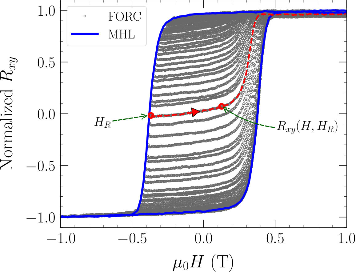

The FORC distribution is acquired through the second-order mixed derivative, as defined by equation 3 :
| (3) |
The FORC distribution was assessed through the application of a locally fitted second-order polynomial surface. A gradient smoothing factor was incorporated into the algorithm to suppress numerical artifacts. Conventionally, FORC diagrams are depicted in terms of the coercivity field () and the interaction field (), which can be derived using and . The resulting FORC diagram is displayed in figure 3b, where a central ridge is observed around and . Figure 3c illustrates the local interaction field distribution of the MRG. A narrow distribution of , with a central point at , emphasizes the lack of any significant interactions (dipolar, etc.) between the elementary units (hysterons) that comprise the MRG. Consequently, in the absence of inter-particle interactions, the overall system can be reasonably approximated using the Stoner-Wohlfarth (SW) model Stoner and Wohlfarth 1948.
The coercive field distribution of the FORC diagram is depicted in figure 3d, with the peak of the distribution centered at . In the absence of interactions, coercive field distribution also represents the switching field distribution (SFD) of hysterons. A statistical analysis of SFD was conducted within the framework of the Preisach model. For this analysis, a pseudo-Voigt distribution is employed, defined as:
| (4) |
where, and are normalized Gaussian and Lorentzian function. is the common FWHM and is peak center. () serves as a weighting factor that transitions the overall profile between pure Gaussian and pure Lorentzian distributions by adjusting the factor from 1 to 0, respectively.
The coercive field distribution within the FORC diagram can be suitably fitted using equation 4. The elongated tail of the coercivity distribution is attributable to the magnetic viscosity resulting from the thermal fluctuations of metastable states. In MRG, magnetic viscosity predominantly stems from the rotation of the magnetization vector, as contributions from domain wall motion are substantially hindered by defects and disorder present within the film Teichert et al. 2021. Therefore, viscosity can be expressed as the sum of exponentially decaying metastable states. Convolution of these states with the pseudo-Voigt function results in the Preisach distribution or switching field distribution (SFD), as demonstrated in equation 5:
|
|
(5) |
here, represents the magnetic viscosity parameter, measured in units of magnetic field. Figure 3d provides clear evidence of a strong agreement between the experimentally obtained coercive field distribution under FORC method and the theoretical prediction provided by the Preisach distribution (equation 5). This finding supports the conclusion that the distribution described by equation 5 can be safely considered as a unique Preisach distribution of the MRG samples. It is worth noting that appropriate normalization methods (amplitude or arial) must be implemented in order to accurately signify the deterministic switching of hysterons. These findings not only contribute to a better understanding of the switching behavior of MRG samples, but also have important implications for the development of more robust models for other similar systems.
Upon obtaining the requisite hysteron distribution, a hysteresis curve for the MRG can be seamlessly derived by integrating this distribution into the Preisach model (equation 2.). Figure 4a demonstrates a remarkable congruence between the experimental AHE hysteresis data obtained at and the fit generated through the Preisach model, with the corresponding resultant Preisach distribution presented in figure 4b. Furthermore, this model has been expanded to encompass out-of-plane hysteresis measurements of MRG at various other temperatures.
Figure 5 illustrates the AHE hysteresis loops and corresponding Preisach distributions at select temperature values, such as , , and . As evidenced by these results, the model captures the experimental intricacies with remarkable precision, thereby underscoring its ability to accurately represent the extensive range of hysteresis observed in MRG using with only a limited number of parameters (). Additional insights into the magnetic properties can also be gleaned from this model.
Figure 6 depicts the variations in the center point () and magnetic viscosity () as functions of temperature for hysteresis curves measured at diverse temperature range. A notably weak dependency of the magnetic viscosity parameter on temperature is observed, which can be ascribed to the dominant influence of anisotropy on the overall energy landscape of MRG. Consequently, any weaker thermodynamic fluctuations exert negligible impact on the static dynamics of the magnetization, causing the magnetic domains of MRG to remain frozen over a wide temperature range.
The relationship between the center point (), which is also known as the sample’s coercivity, and temperature is characterized by two distinct regimes. At elevated temperatures, the coercive field experiences an increase due to the diminishing net moment as it approaches the compensation point (); conversely, at lower temperatures, the rise in effective anisotropy prevails.
III.2 Torque model
In the investigation of magnetization dynamics, employing the macrospin approximation serves as a highly effective approach for analysis. In this approximation, the spatial variation of the magnetization remains constant throughout the equation of motion. The static and quasi-static magnetization dynamics of MRG can be accurately represented under the macrospin approximation, as it accounts for the absence of hysteron interaction, which is clearly illustrated in figure 3c. The torque model is constructed based on the macrospin approximation, where the equilibrium direction of the magnetization is determined by counterbalancing the torque that arises from anisotropy fields with the Zeeman torque. For the tetragonal MRG system, the torque balance equation can be efficiently derived from the magnetic anisotropy free energy expression, in which and represent the polar and azimuthal angles of the magnetization vector :
| (6) | |||||
Here, the first and second-order uniaxial out-of-plane anisotropy constants are denoted by and , respectively, while signifies the four-fold in-plane anisotropy constant. By evaluating the extrema of equation 6 with respect to and , the equilibrium magnetization direction can be determined. For instance, the polar equilibrium position can be ascertained by solving the subsequent equation:
| (7) | |||||
In the aforementioned equation, it is assumed that the in-plane anisotropy () is relatively weak; therefore, M adheres to the applied magnetic field (H) along the azimuthal direction with a slight delay, i.e., . Here, the polar angle and the azimuthal angle of the applied magnetic field are represented by and , respectively. In this work, we utilize the anomalous Hall effect (AHE) to examine the anisotropy constants, which is particularly sensitive to the out-of-plane component of the Mn4c moment, therefore:
| (8) |
where, denotes the AHE voltage when the magnetization (M) is aligned with the normal to the sample (), and represents the normalized AHE voltage. Consequently, the equilibrium condition (equation 7) is reduced to:
| (9) | |||||
To determine the values of , , and , rotational scans were conducted in various geometric configurations.
It is important to recognize that the recorded transverse resistance consists of five distinct contributions, which include: the ordinary Hall effect (OHE), the anomalous Hall effect (AHE), the planar Hall effect (PHE), the ordinary Nernst effect (ONE), and the anomalous Nernst effect (ANE). These contributions are represented in equation 10 Nagaosa et al. 2010; Miyasato et al. 2007:
| (10) |
In the context of MRG, the ordinary Nernst effect ( ) and the anomalous Nernst effect ( ) were effectively minimized by employing an exceedingly small input bias current signal (). This approach ensured the absence of any significant thermal gradient within the observed sample. To further mitigate the temperature gradient across the Hall bar, temperatures were stabilized using a helium partial pressure () within a PPMS tool. The sample was carefully rotated at a very slow rate to minimize temperature destabilization that could arise from friction within the sample’s rotator gears. The ordinary Hall effect ( ) was determined by measuring the slope of the AHE at high magnetic fields (), as illustrated in figure 7a. The Hall coefficient calculated for MRG yielded a value of m3 C-1, which corresponds to a carrier concentration cm-3. In MRG, the Hall effect is predominantly governed by the minority carrier at the Fermi level due to the material’s high spin-polarization Kurt et al. 2014; Fowley et al. 2018.
The planar Hall effect () was evaluated by rotating the magnetic field within the plane of the sample. Figure 7b displays the anisotropic magneto-resistance (AMR) and the planar Hall effect (PHE) measured at room temperature in the presence of a magnetic field with a value of . The observed PHE is three orders of magnitude smaller than the recorded AHE, thus allowing it to be safely disregarded from equation 10. As a result, the primary dominant contribution to the transverse Hall resistance is due to the AHE. Nevertheless, OHE has also been considered in the model to acknowledge its significant contribution, particularly at high applied magnetic fields.
To investigate the out-of-plane anisotropy constants ( and ), the AHE was conducted in the measurement geometry depicted in figure 8a. In this configuration, the sample was rotated in such a way that the applied magnetic field effectively rotated within the -plane. Figure 8b presents the three rotational AHE loops measured at T = 300 K, under constant applied magnetic fields of , , and .
The acquired data exhibit two distinct regimes: the first regime showcases a continuous change in the resistance (non-hysteretic segments, for ∘, ∘ and in the vicinity of ∘), attributable to the smooth coherent rotation of the magnetization against the anisotropy field, while the second regime displays an abrupt change in the resistance (hysteretic segments, for ) due to the switching of the magnetic moment from out-of-plane to in-plane or vice versa. The non-hysteretic portions of the data were fitted using the torque model. Since the anisotropy constants are independent of the applied external field (at least up to the first order), the non-hysteretic segments of the data should be modelled using common fitting parameters. Figure 8c illustrates the recorded data alongside the corresponding best fits utilizing common anisotropy parameters. The data align well with the model, yielding anisotropy constants of and , where denotes the magnitude of saturation magnetization. The sample’s saturation magnetization, obtained from SQUID measurement, is . Consequently, the first and second order out-of-plane anisotropy constants of MRG are J m-3 and J m-3, respectively. It is crucial to note that in this measurement geometry, the AHE is insensitive to in-plane anisotropy due to the absence of azimuthal rotation of magnetization. The in-plane anisotropy constant () can be examined in a measurement geometry where the azimuthal direction of magnetization is varied.
Progressing with the study, the in-plane anisotropy was examined using the AHE in the measurement geometry depicted in figure 8d. In this configuration, the sample was rotated in such a way that the applied magnetic field effectively rotated within the plane of the sample (-plane). The presence of in-plane anisotropy causes the AHE signal to oscillate as a function of the azimuthal angle () of the magnetization, revealing the four-fold anisotropy of MRG. Figure 8e and 8f display the scans obtained at when constant magnetic fields of and were applied in the plane of the sample, respectively. The unequal amplitude of oscillation arises from a small offset ( ) of the sample from the -plane, which subsequently causes sample wobbling during rotation and introduces an additional term – a non-zero normal component – affecting the magnetization vector position . The equilibrium position of the magnetization vector, under the influence of the external magnetic field, is numerically obtained using the torque model with a correction for wobbling taken into consideration (the implementation involved employing Rodrigues’ rotation formula, which utilizes the appropriate axis of rotation). The extracted value of the in-plane anisotropy constant is , or J m-3, which is an order of magnitude smaller than the out-of-plane anisotropy constants and . It is noteworthy that an increase in field strength results in a more pronounced hysteresis of AHE in the in-plane configuration (comparing figure 8e and 8f). This phenomenon occurs because, at sufficiently high magnetic fields, the sample wobbling leads to partial switching of magnetic moments. Modeling such complex data, where both coherent rotation and magnetization switching take place, can be accomplished by combining both the Preisach and torque models.
III.3 Combined Preisach and torque (CPT) model
III.3.1 In-plane field hysteresis loop
The intricate quasi-static magnetization dynamics can be elucidated by combining the torque and Preisach models, wherein the magnetic moment exhibits both coherent rotation and abrupt switching events under the influence of suitable stimuli. One such mixed behavior can also be observed when a high magnetic field is swept within the plane of the sample. To examine such dynamics, AHE was measured in the measurement geometry depicted in figure 9a. In this setup, the magnetic field was swept within the plane of the sample (along the -axis) from . The recorded AHE signal exhibits a combination of hysteretic and rotational behavior, as shown in figure 9b. Due to an unavoidable minor offset () of the sample while mounting it on the rotary stage of the PPMS, the applied magnetic field does not lie exactly within the plane of the sample (see the inset of figure 9b).
An offset of approximately was present, the exact offset value can be determined by fitting the AHE data. As a result, the AHE signal has two distinct regimes: (i) when the magnetic field (H) forms an acute angle with the normal to the sample (), a coherent rotation of the magnetization vector is observed; and (ii) when the magnetic field makes an obtuse angle with the normal ( ), the switching of the magnetic moment occurs when the field projection surpasses the coercive field. It should be noted that the coercive field in this scenario is scaled according to equation 11:
| (11) |
here, represents the coercivity of the MRG sample when the magnetic field is applied along the direction normal to the sample plane ().
A comprehensive trajectory of magnetization under the influence of the applied magnetic field is meticulously demonstrated in figure 9b. This representation encompasses the combined behaviour of the rotation of magnetic moments and their corresponding switching events, which can be effectively described through equation 12;
| (12) |
where, and denote the respective contributions arising from the torque model (as explicated in equation 9 ) and the Preisach model (as detailed in equation 5). To determine the solution for equation 12, the Levenberg-Marquardt algorithm was employed, while maintaining the anisotropy constants at a fixed value of and at . The resultant estimated curve, in conjunction with the data, is displayed in figure 9b, which reveals an exceptional congruence with the gathered data. Furthermore, figure 9c depicts the estimated hysteron distribution for the corresponding AHE curve, with the central point of distribution () determined to be . Notably, this distribution curve also exhibits a strong resemblance to the hysteron distribution curve obtained when the magnetic field is applied perpendicular to the sample (as shown in figure 4b), with the field axis scaled according to equation 11. This consistency highlights the robustness of the analysis and further validates the effectiveness of the model.
Though the combined Preisach and torque (CPT) model, as delineated by equation 12, effectively predicts the intricate magnetization dynamics, implementing this equation to depict complex quasi-static magnetic dynamics presents a considerable computational challenge due to the multiparameter nature of the equation. Nevertheless, the awareness that the Preisach distribution for a specific temperature can be independently determined through a pure switching event (out-of-plane hysteresis curve) allows for further simplification of the combined model. This is achieved by further considering an effective out-of-plane anisotropy field () to resolve the pure torque model component. The rationale for utilizing an effective anisotropy field stems from the fact that MRG exhibits substantial and dominating out-of-plane anisotropy, which is also evident from the steep square hysteresis loop observed when the field is swept perpendicular to the sample (figure 7a). Under this approximation, the equilibrium position of magnetization () can be attained by counterbalancing the torques acting upon it, (equation 13 )
| (13) |
where, and represent the effective out-of-plane anisotropy field and the applied external magnetic field, respectively. In figure 9d, the data and corresponding fit are presented, which utilize the model with a single free parameter ( ) and the Preisach model that has been determined previously. The calculated value from the fitting is . The model captures all details of the AHE, thereby validating the proposed approximation. It is important to note that by comparing figures 9b and 9d, the distinction between the two models can be discerned. At high magnetic field values (), the effective anisotropy field model slightly deviates from the data and does not accurately capture the curvature of the data as effectively as the complete model (figure 9b). This is due to the model’s assumption of a unique fixed value for all orientations. In contrast, the magnitude of for a tetragonal crystal system relies on the magnetization direction, and its magnitude typically decreases as deviates from the out-of-plane direction (easy-axis). Consequently, a is necessary to capture the data in greater detail for all possible magnetic field values. Nonetheless, it is adequate to assume that a single fixed performs remarkably well, at least up to the magnetic field strength employed in this study (). This approximation offers a significant advantage in describing complex magnetization dynamics by substantially reducing the number of free parameters in the model.
III.3.2 Out-of-plane rotational hysteresis loop
The efficacy of the CPT model is further substantiated by applying it to magnetization dynamics derived from out-of-plane rotational hysteresis curves, as illustrated in figure 10. In this experiment, AHE curves were acquired utilizing the measurement geometry shown in figure 10a. This setup involves rotating a constant applied magnetic field within the -plane, causing the equilibrium position of the magnetic moment () to reside within the same plane. A collection of AHE data, recorded at applied magnetic field values of , and , and their corresponding CPT fits, are displayed in figures 10b, 10c, and 10d, respectively. The CPT model well-describes the dataset across all applied magnetic fields.
It is important to note that as the magnitude of the applied magnetic field escalates, the hysteretic contribution to the AHE starts to decrease relative to the non-hysteretic contribution, resulting in a reduced hysteretic width. In cases where the field strength reaches exceptionally high levels, the Zeeman term prevails over the anisotropy term, thereby causing the magnetization to effectively align with the magnetic field direction. Consequently, at a field, the hysteresis width has virtually disappeared (figure 10d). In the context of the current CPT fitting approach, all parameters, including the effective out-of-plane anisotropy field () and the coefficients of hysteron distribution (), are maintained as constant values. These parameters have been previously determined through the fitting of other AHE curves, as elaborated upon in the preceding sections. As a result, the derived fitting curve successfully captures both the hysteretic and non-hysteretic aspects of the AHE curve with remarkable precision, for both low () and high applied magnetic fields (), while virtually eliminating the need for free parameters.
IV Conclusion
In this work, we have developed a comprehensive methodology for determining the various magnetic anisotropy constants of low-moment MRG thin films. To achieve this, we initially investigated hysteretic phenomena using the Preisach model, also known as the hysteron model. The applicability of the Preisach model was subsequently experimentally verified through the implementation of the first-order reversal curves (FORC) method, which enabled us to identify the unique hysteron distribution of the sample under investigation. The FORC method provided crucial insights, specifically highlighting the absence of long-range magnetic interactions within the hysterons, which allowed for the utilization of the macrospin model (Stoner-Wohlfarth model) to describe the quasi-static magnetization dynamics of MRG. Furthermore, the Preisach model confirmed that MRG samples exhibit relatively weak variations in magnetic viscosity with temperature, signifying the presence of a frozen domain structure. To determine the anisotropy constants of the MRG samples, we employed a detailed torque model within the macrospin approximation framework. Anomalous Hall effect (AHE) measurements were carried out in various suitable geometries, which facilitated the deduction of out-of-plane anisotropy constants J m-3 ( T) and J m-3 ( T), and an in-plane anisotropy constant J m-3 ( T) through data fitting with the torque model. Additionally, we successfully investigated more complex quasi-static magnetization dynamics, characterized by the combination of hysteretic and non-hysteretic components in AHE, using a combined Preisach and torque (CPT) model with virtually no free parameters. Our study demonstrates the efficacy of this methodology not only in determining the magnetic anisotropy of low moment magnetic samples (MRG), but also in explaining other complex magnetization dynamics within a unified model. The proposed method can be readily extended to other magnetic systems that lack hysteronic interactions, exhibit narrow hysteron distributions, and display frozen-domain behaviour. This comprehensive approach will undoubtedly prove valuable in studying both linear and non-linear quasi-static magnetization dynamics of MRG in external fields and/or current-induced effective fields resulting from spin-orbit torque/spin-transfer torque.
Acknowledgements
A.J., S.L., G.P., K.R., J.M.D.C and P.S. acknowledge funding from TRANSPIRE FET Open H2020 and SFI, AMBER and MANIAC programmes.
References
- Chappert et al. (2007) C. Chappert, A. Fert, and F. N. Van Dau, The emergence of spin electronics in data storage, Nature materials 6, 813 (2007).
- Jungwirth et al. (2016) T. Jungwirth, X. Marti, P. Wadley, and J. Wunderlich, Antiferromagnetic spintronics, Nature nanotechnology 11, 231 (2016).
- Baltz et al. (2018) V. Baltz, A. Manchon, M. Tsoi, T. Moriyama, T. Ono, and Y. Tserkovnyak, Antiferromagnetic spintronics, Rev. Mod. Phys. 90, 015005 (2018).
- Khvalkovskiy et al. (2013) A. Khvalkovskiy, D. Apalkov, S. Watts, R. Chepulskii, R. Beach, A. Ong, X. Tang, A. Driskill-Smith, W. Butler, P. Visscher, et al., Basic principles of STT-MRAM cell operation in memory arrays, Journal of Physics D: Applied Physics 46, 074001 (2013).
- Demidov et al. (2012) V. E. Demidov, S. Urazhdin, H. Ulrichs, V. Tiberkevich, A. Slavin, D. Baither, G. Schmitz, and S. O. Demokritov, Magnetic nano-oscillator driven by pure spin current, Nature materials 11, 1028 (2012).
- Wadley et al. (2016) P. Wadley, B. Howells, J. Železnỳ, C. Andrews, V. Hills, R. P. Campion, V. Novák, K. Olejník, F. Maccherozzi, S. Dhesi, et al., Electrical switching of an antiferromagnet, Science 351, 587 (2016).
- Pickett (1998) W. E. Pickett, Spin-density-functional-based search for half-metallic antiferromagnets, Phys. Rev. B 57, 10613 (1998).
- Galanakis et al. (2007) I. Galanakis, K. Özdoğan, E. Şaşıoğlu, and B. Aktaş, Ab initio design of half-metallic fully compensated ferrimagnets: The case of (, As, Sb, and Bi), Phys. Rev. B 75, 172405 (2007).
- Kurt et al. (2014) H. Kurt, K. Rode, P. Stamenov, M. Venkatesan, Y. C. Lau, E. Fonda, and J. M. Coey, Cubic Mn2Ga Thin films: Crossing the spin gap with ruthenium, Physical Review Letters 112, 2 (2014).
- Siewierska et al. (2021) K. E. Siewierska, G. Atcheson, A. Jha, K. Esien, R. Smith, S. Lenne, N. Teichert, J. O’Brien, J. M. D. Coey, P. Stamenov, and K. Rode, Magnetic order and magnetotransport in half-metallic ferrimagnetic thin films, Phys. Rev. B 104, 064414 (2021).
- Banerjee et al. (2020) C. Banerjee, N. Teichert, K. Siewierska, Z. Gercsi, G. Atcheson, P. Stamenov, K. Rode, J. Coey, and J. Besbas, Single pulse all-optical toggle switching of magnetization without gadolinium in the ferrimagnet Mn2RuxGa, Nature communications 11, 1 (2020).
- Teichert et al. (2021) N. Teichert, G. Atcheson, K. Siewierska, M. N. Sanz-Ortiz, M. Venkatesan, K. Rode, S. Felton, P. Stamenov, and J. Coey, Magnetic reversal and pinning in a perpendicular zero-moment half-metal, Physical Review Materials 5, 034408 (2021).
- Van Leuken and De Groot (1995) H. Van Leuken and R. De Groot, Half-metallic antiferromagnets, Physical review letters 74, 1171 (1995).
- Betto et al. (2015) D. Betto, N. Thiyagarajah, Y.-C. Lau, C. Piamonteze, M.-A. Arrio, P. Stamenov, J. Coey, and K. Rode, Site-specific magnetism of half-metallic Mn2RuxGa thin films determined by X-ray absorption spectroscopy, Physical Review B 91, 094410 (2015).
- Fowley et al. (2018) C. Fowley, K. Rode, Y.-C. Lau, N. Thiyagarajah, D. Betto, K. Borisov, G. Atcheson, E. Kampert, Z. Wang, Y. Yuan, S. Zhou, J. Lindner, P. Stamenov, J. M. D. Coey, and A. M. Deac, Magnetocrystalline anisotropy and exchange probed by high-field anomalous Hall effect in fully compensated half-metallic thin films, Physical Review B 98, 220406 (2018).
- Žic et al. (2016) M. Žic, K. Rode, N. Thiyagarajah, Y. C. Lau, D. Betto, J. M. Coey, S. Sanvito, K. J. O’Shea, C. A. Ferguson, D. A. Maclaren, and T. Archer, Designing a fully compensated half-metallic ferrimagnet, Physical Review B 93, 1 (2016), arXiv:1511.07923 .
- Siewierska et al. (2018) K. Siewierska, N. Teichert, R. Schäfer, and J. Coey, Imaging domains in a zero-moment half metal, IEEE Transactions on Magnetics 55, 1 (2018).
- Troncoso et al. (2019) R. E. Troncoso, K. Rode, P. Stamenov, J. M. D. Coey, and A. Brataas, Antiferromagnetic single-layer spin-orbit torque oscillators, Phys. Rev. B 99, 054433 (2019).
- Awari et al. (2016) N. Awari, S. Kovalev, C. Fowley, K. Rode, R. A. Gallardo, Y. C. Lau, D. Betto, N. Thiyagarajah, B. Green, O. Yildirim, J. Lindner, J. Fassbender, J. M. Coey, A. M. Deac, and M. Gensch, Narrow-band tunable terahertz emission from ferrimagnetic Mn3-xGa thin films, Applied Physics Letters 109, 10.1063/1.4958855 (2016).
- Fan et al. (2007) X. Fan, D. Xue, C. Jiang, Y. Gong, and J. Li, An approach for researching uniaxial anisotropy magnet: Rotational magnetization, Journal of Applied Physics 102, 123901 (2007).
- Endo et al. (2000) Y. Endo, O. Kitakami, S. Okamoto, and Y. Shimada, Determination of first and second magnetic anisotropy constants of magnetic recording media, Applied Physics Letters 77, 1689 (2000).
- Jagla (2005) E. A. Jagla, Hysteresis loops of magnetic thin films with perpendicular anisotropy, Physical Review B 72, 094406 (2005).
- Okamoto (1983) K. Okamoto, A new method for analysis of magnetic anisotropy in films using the spontaneous hall effect, Journal of magnetism and magnetic materials 35, 353 (1983).
- Sato et al. (2011) H. Sato, M. Pathak, D. Mazumdar, X. Zhang, G. Mankey, P. LeClair, and A. Gupta, Anomalous Hall effect behavior in (100) and (110) CrO2 thin films, Journal of Applied Physics 109, 103907 (2011).
- Suran et al. (1999) G. Suran, M. Naili, H. Niedoba, F. Machizaud, O. Acher, and D. Pain, Magnetic and structural properties of Co-rich CoFeZr amorphous thin films, Journal of magnetism and magnetic materials 192, 443 (1999).
- Berling et al. (2006) D. Berling, S. Zabrocki, R. Stephan, G. Garreau, J. Bubendorff, A. Mehdaoui, D. Bolmont, P. Wetzel, C. Pirri, and G. Gewinner, Accurate measurement of the in-plane magnetic anisotropy energy function Ea () in ultrathin films by magneto-optics, Journal of magnetism and magnetic materials 297, 118 (2006).
- Cowburn et al. (1997) R. Cowburn, A. Ercole, S. Gray, and J. Bland, A new technique for measuring magnetic anisotropies in thin and ultrathin films by magneto-optics, Journal of applied physics 81, 6879 (1997).
- Preisach (1935) F. Preisach, Über die magnetische nachwirkung, Zeitschrift für physik 94, 277 (1935).
- Della Torre (1986) E. Della Torre, Magnetization calculation of fine particles, IEEE Transactions on Magnetics 22, 484 (1986).
- Kádár et al. (1989) G. Kádár, E. Kisdi-Koszo, L. Kiss, L. Potocky, M. Zatroch, and E. Della Torre, Bilinear product preisach modeling of magnetic hysteresis curves, IEEE Transactions on Magnetics 25, 3931 (1989).
- Fuzi (2003) J. Fuzi, Analytical approximation of preisach distribution functions, IEEE transactions on magnetics 39, 1357 (2003).
- Henze and Rucker (2002) O. Henze and W. M. Rucker, Identification procedures of preisach model, IEEE Transactions on magnetics 38, 833 (2002).
- Galinaitis et al. (2001) W. S. Galinaitis, D. S. Joseph, and R. C. Rogers, Parameter identification for preisach models of hysteresis, in International Design Engineering Technical Conferences and Computers and Information in Engineering Conference, Vol. 80289 (American Society of Mechanical Engineers, 2001) pp. 1409–1417.
- Mayergoyz (1986) I. Mayergoyz, Mathematical models of hysteresis, IEEE Transactions on magnetics 22, 603 (1986).
- Chiriac et al. (2007) H. Chiriac, N. Lupu, L. Stoleriu, P. Postolache, and A. Stancu, Experimental and micromagnetic first-order reversal curves analysis in NdFeB-based bulk “exchange spring”-type permanent magnets, Journal of magnetism and magnetic materials 316, 177 (2007).
- Chen et al. (2014) P.-A. Chen, C.-Y. Yang, S.-J. Chang, M.-H. Lee, N.-K. Tang, S.-C. Yen, and Y.-C. Tseng, Soft and hard natures of Nd2Fe14B permanent magnet explored by first-order-reversal-curves, Journal of magnetism and magnetic materials 370, 45 (2014).
- Roberts et al. (2000) A. P. Roberts, C. R. Pike, and K. L. Verosub, First-order reversal curve diagrams: A new tool for characterizing the magnetic properties of natural samples, Journal of Geophysical Research: Solid Earth 105, 28461 (2000).
- Muxworthy and Roberts (2007) A. R. Muxworthy and A. P. Roberts, First‐order reversal curve (forc) diagrams, in Encyclopedia of Geomagnetism and Paleomagnetism, edited by D. Gubbins and E. Herrero-Bervera (Springer Netherlands, Dordrecht, 2007) pp. 266–272.
- Béron et al. (2006) F. Béron, L. Clime, M. Ciureanu, D. Ménard, R. W. Cochrane, and A. Yelon, First-order reversal curves diagrams of ferromagnetic soft nanowire arrays, IEEE transactions on magnetics 42, 3060 (2006).
- Béron et al. (2008) F. Béron, L.-P. Carignan, D. Ménard, and A. Yelon, Magnetic behavior of Ni/Cu multilayer nanowire arrays studied by first-order reversal curve diagrams, IEEE Transactions on Magnetics 44, 2745 (2008).
- Pike et al. (1999) C. R. Pike, A. P. Roberts, and K. L. Verosub, Characterizing interactions in fine magnetic particle systems using first order reversal curves, Journal of Applied Physics 85, 6660 (1999).
- Stancu et al. (2003) A. Stancu, D. Ricinschi, L. Mitoseriu, P. Postolache, and M. Okuyama, First-order reversal curves diagrams for the characterization of ferroelectric switching, Applied Physics Letters 83, 3767 (2003).
- Ramírez et al. (2009) J.-G. Ramírez, A. Sharoni, Y. Dubi, M. Gómez, and I. K. Schuller, First-order reversal curve measurements of the metal-insulator transition in : Signatures of persistent metallic domains, Physical Review B 79, 235110 (2009).
- Diao et al. (2012) Z. Diao, N. Decorde, P. Stamenov, K. Rode, G. Feng, and J. Coey, Magnetization processes in micron-scale (CoFe/Pt)n multilayers with perpendicular anisotropy: First-order reversal curves measured by extraordinary Hall effect, Journal of Applied Physics 111, 07B538 (2012).
- Stoner and Wohlfarth (1948) E. C. Stoner and E. Wohlfarth, A mechanism of magnetic hysteresis in heterogeneous alloys, Philosophical Transactions of the Royal Society of London. Series A, Mathematical and Physical Sciences 240, 599 (1948).
- Nagaosa et al. (2010) N. Nagaosa, J. Sinova, S. Onoda, A. H. MacDonald, and N. P. Ong, Anomalous hall effect, Rev. Mod. Phys. 82, 1539 (2010).
- Miyasato et al. (2007) T. Miyasato, N. Abe, T. Fujii, A. Asamitsu, S. Onoda, Y. Onose, N. Nagaosa, and Y. Tokura, Crossover behavior of the anomalous hall effect and anomalous nernst effect in itinerant ferromagnets, Phys. Rev. Lett. 99, 086602 (2007).