Identifiability Guarantees for Causal Disentanglement
from Soft Interventions
Abstract
Causal disentanglement aims to uncover a representation of data using latent variables that are interrelated through a causal model. Such a representation is identifiable if the latent model that explains the data is unique. In this paper, we focus on the scenario where unpaired observational and interventional data are available, with each intervention changing the mechanism of a latent variable. When the causal variables are fully observed, statistically consistent algorithms have been developed to identify the causal model under faithfulness assumptions. We here show that identifiability can still be achieved with unobserved causal variables, given a generalized notion of faithfulness. Our results guarantee that we can recover the latent causal model up to an equivalence class and predict the effect of unseen combinations of interventions, in the limit of infinite data. We implement our causal disentanglement framework by developing an autoencoding variational Bayes algorithm and apply it to the problem of predicting combinatorial perturbation effects in genomics.
1 Introduction
The discovery of causal structure from observational and interventional data is important in many fields including statistics, biology, sociology, and economics [Meinshausen et al., 2016; Glymour et al., 2019]. Directed acyclic graph (DAG) models enable scientists to reason about causal questions, e.g., predicting the effects of interventions or determining counterfactuals [Pearl, 2009]. Traditional causal structure learning has considered the setting where the causal variables are observed [Heinze-Deml et al., 2018]. While sufficient in many applications, this restriction is limiting in most regimes where the available datasets are either perceptual (e.g., images) or very-high dimensional (e.g., the expression of human genes). In an imaging dataset, learning a causal graph on the pixels themselves would not only be difficult since there is no common coordinate system across images (pixel in one image may have no relationship with pixel in another image) but of questionable utility due to the relative meaninglessness of interventions on individual pixels. Similar problems are also present when working with very high-dimensional data. For example, in a gene-expression dataset, subsets of genes (e.g. belonging to the same pathway) may function together to induce other variables and should therefore be aggregated into one causal variable.
These issues mean that the causal variables need to be learned, instead of taken for granted. The recent emerging field of causal disentanglement [Cai et al., 2019; Xie et al., 2022; Kivva et al., 2021] seeks to remedy these issues by recovering a causal representation in latent space, i.e., a small number of variables that are mapped to the observed samples in the ambient space via some mixing map . This framework holds the potential to learn more semantically meaningful latent factors than current approaches, in particular factors that correspond to interventions of interest to modelers. Returning to the image and the genomic examples, latent factors could, for example, be abstract functions of pixels (corresponding to objects) or groups of genes (corresponding to pathways).
Despite a recent flurry of interest, causal disentanglement remains challenging. First, it inherits the difficulties of causal structure learning where the number of causal DAGs grows super-exponentially in dimension. Moreover, since we only observe the variables after the unknown mixing function but never the latent variables, it is generally impossible to recover the latent causal representations with only observational data. Under the strong assumption that the causal DAG is the empty graph, such unidentifiability from observational data has been discussed in previous disentanglement works [Khemakhem et al., 2020].
However, recent advances in many applications enable access to interventional data. For example, in genomics, researchers can perturb single or multiple genes through CRISPR experiments [Dixit et al., 2016]. Such interventional data can be used to identify the causal variables and learn their causal relationships. When dealing with such data, it is important to note that single-cell RNA sequencing and other biological assays often destroy cells in the measurement process. Thus, the available interventional data is unpaired: for each cell, one only obtains a measurement under a single intervention.
In this work, we establish identifiability for soft interventions on general structural causal models (SCMs), when the latent causal variables are observed through a class of (potentially non-linear) polynomial mixing functions proposed by [Ahuja et al., 2022b]. Prior works [Tian and Pearl, 2001; Hauser and Bühlmann, 2012; Yang et al., 2018b] show that the causal model can be identified under faithfulness assumptions, when all the causal variables are observed. We here demonstrate that idenfiability can still be achieved when the causal variables are unobserved under a generalized notion of faithfulness. The identifiability is up to an equivalence class and guarantees that we can predict the effect of unseen combinations of interventions, in the limit of infinite data. It then remains to design an algorithmic approach to estimate the latent causal representation from data. We propose an approach based on autoencoding variational Bayes [Kingma and Welling, 2013], where the decoder is composed of a deep SCM (DSCM) [Pawlowski et al., 2020] followed by a deep mixing function. Finally, we apply our approach to a real-world genomics dataset to find genetic programs and predict the effect of unseen combinations of genetic perturbations.
1.1 Related Work
Identifiable Representation Learning. The identifiability of latent representations from observed data has been a subject of ongoing study. Common assumptions are that the latent variables are independent [Comon, 1994], are conditionally independent given some observed variable [Hyvarinen et al., 2019; Khemakhem et al., 2020], or follow a known distribution [Zimmermann et al., 2021]. In contrast, we do not make any independence assumptions on the latent variables or assume we know their distribution. Instead, we assume that the variables are related via a causal DAG model, and we use data from interventions in this model to identify the representation.
Causal Structure Learning. The recovery of a causal DAG from data is well-studied for the setting where the causal representation is directly observed [Heinze-Deml et al., 2018]. Methods for this task take a variety of approaches, including exact search [Cussens, 2020] and greedy search [Chickering, 2002] to maximize a score such as the posterior likelihood of the DAG, or an approximation thereof. These scores can be generalized to incorporate interventional data [Wang et al., 2017; Yang et al., 2018b; Kuipers and Moffa, 2022], and methods can often be naturally extended by considering an augmented search space [Mooij et al., 2020]. Indeed, interventional data is generally necessary for identifiability without further assumptions on the functions relating variables [Squires and Uhler, 2022].
Causal Disentanglement. The task of identifying a causal DAG over latent causal variables is less well-studied, but has been the focus of much recent work [Cai et al., 2019; Xie et al., 2022; Kivva et al., 2021]. These works largely do not consider interventions, and thus require restrictions on functional forms as well as structural assumptions on the map from latent to observed variables. Among works that do not restrict the map, [Ahuja et al., 2022a] and [Brehmer et al., 2022] assume access to paired counterfactual data. In contrast, we consider only unpaired data, which is more common in applications such as biology [Stark et al., 2020]. Unpaired interventional data is considered by [Ahuja et al., 2022b], [Squires et al., 2023], and as a special case of [Liu et al., 2022]. These works do not impose structural restrictions on the map from latent to observed variables but assume functional forms of the map, such as linear or polynomial. Our work builds on and complements these results by providing identifiability for soft interventions and by offering a learning algorithm based on variational Bayes. We remark here that the task of causal disentanglement is sometimes called causal representation learning in literature. We adopted the term causal disentanglement mainly following [Kaddour et al., 2022], as causal representation learning also includes methods such as Invariant Risk Minimization (IRM) [Arjovsky et al., 2019] which do not completely learn latent variables. We discuss contemporaneous related work in Section 7.
2 Problem Setup
We now formally introduce the causal disentanglement problem of identifying latent causal variables and causal structure between these variables. We consider the observed variables as being generated from latent variables through an unknown deterministic (potentially non-linear) mixing function . In the observational setting, the latent variables follow a joint distribution that factorizes according to an unknown directed acyclic graph (DAG) with nodes . Concisely, we have the following data-generating process:
| (1) |
where denotes the parents of in . We also use , and to denote the children, descendants and ancestors of in . Let denote the induced distribution over .

We consider atomic (i.e., single-node) interventions on the latent variables. While our main focus is on general types of soft interventions, our proof also applies to hard interventions. In particular, an intervention with target modifies the joint distribution by changing the conditional distribution . A hard intervention sets the conditional distribution as , removing the dependency of on , whereas a soft intervention is allowed to preserve this dependency but changes the mechanism into . An example of a soft intervention is as a shift intervention [Rothenhäusler et al., 2015; Zhang et al., 2021], which modifies the conditional distribution as for some shift value . In the following, we will use to denote the interventional distribution, where for . We denote the induced distribution over by . In cases where the referred random variable is clear from the context, we abbreviate the subscript and use instead.
We consider the setting where we have unpaired data from observational and interventional distributions, i.e., . Here, denotes samples of where ; denotes samples of where . We focus on the scenario where we have at least one intervention per latent node. In the worst case, one intervention per node is necessary for identifiability in linear SCMs [Squires et al., 2023]. We note that having at least one intervention per latent node is a strict generalization of having exactly one intervention per latent node, since we assume no knowledge of which interventions among target the same node. Throughout the paper, we assume latent variables are unobserved and their dimension , the DAG , and the interventional targets of are unknown. The goal is to identify these given samples of in .
3 Equivalence Class for Causal Disentanglement
In this section, we characterize the equivalence class for causal disentanglement, i.e., the class of latent models that can generate the same observed samples of in . Since we only have access to this data, the latent model can only be identified up to this equivalence class.
First, note that the data-generation process is agnostic to the re-indexing of latent variables, provided that we change the mixing function to reflect such re-indexing. More precisely, consider an arbitrary permutation of . Denote and as the mixing function such that . We define as the DAG with nodes in and edges if and only if . Then the following data-generating process,
satisfies . The same argument holds when is generated from an interventional distribution , where this process generates the same when is sampled from . Here is such that and the mechanism .
We would also observe the same data if each is affinely transformed into for constants and and the mixing function is rescaled element-wise to accommodate this transformation. To account for these two types of equivalences, we define the following notion of causal disentanglement (CD) equivalence class.
Definition 1 (CD-Equivalence).
Two sets of variables, and are CD-equivalent if and only if there exists a permutation of , non-zero constants , and such that
The same definition applies to and , where we say they are CD-equivalent if and only if , and for some permutation .
For simplicity, we refrain from talking about transformations on the mixing function and mechanisms of latent variables. These can be obtained once are identified. In particular, is the map from to the observed ; and the joint distribution (and ) can be decomposed with respect to to obtain the mechanisms (and ).
4 Identifiability Results
In this section, we present our main results, namely the identifiability guarantees for causal disentanglement from soft interventions. For this discussion, we consider the infinite-data regime where enough samples are obtained to exactly determine the observational and interventional distributions . Detailed proofs are deferred to Appendices A and B.
4.1 Preliminaries
Following [Ahuja et al., 2022b], we pose assumptions on the support of and on the function class of the map . Our support assumption is for example satisfied under the common additive Gaussian structural causal model [Peters et al., 2017], and our assumption on the function class is for example satisfied if is linear and injective (Lemma 2 in Appendix A), a setting considered in many identifiability works (e.g., [Comon, 1994; Ahuja et al., 2021; Squires et al., 2023]).
Assumption 1.
Let be a -dimensional random vector. Following [Ahuja et al., 2022b], we assume that the interior of the support of is a non-empty subset of , and that is a full row rank polynomial.11 1 There exists some integer , a full row rank and a vector such that , where denotes the size- vector with degree- polynomials of as its entries.
Under this assumption, the authors in [Ahuja et al., 2022b] showed that if is known, is identifiable up to a linear transformation. This remains true when is unknown, as summarized in the following lemma.
Lemma 1.
Under Assumption 1, we can identify the dimension of as well as its linear transformation for some non-singular matrix and vector . In fact, with observational data, we can only identify up to such linear transformations.
Denote all pairs of that satisfy this assumption as . The proof of this lemma is provided by solving the following constrained optimization problem:
In other words, let be the smallest dimension such that there exists a pair of in that generates the observational distribution . Then and we recover the latent factors up to linear transformation. The intuition is that (1) the support with non-empty interior guarantees that we can identify by checking its geometric dimension, and (2) the full-rank polynomial assumption ensures that we search for (and consequently ) in a constrained subspace.
On the other hand, to show we cannot identify more than linear transformations, we construct a mixing function for such that the induced distribution is the same under both representations. This also means that we cannot identify the underlying DAG up to any nontrivial equivalence class; we give an example showing that any causal DAG can explain the observational data in Appendix A. Next, we discuss how identifiability can be improved with interventional data.
4.2 Identifying ancestral relations
Lemma 1 guarantees identifiability up to linear transformations from solely observational data. This reduces the problem to the case where an unknown invertible linear mixing of the latent variables is observed. Without loss of generality, we thus work with this reduction for the remainder of the section.
When the causal variables are fully observed, we can identify causal relationships from the changes made by interventions [Tian and Pearl, 2001]. In particular, an intervention on a node will not alter the marginals of its non-descendants as compared to the observational distribution, i.e., for and . However, it is possible that for some in degenerate cases where the change made by is canceled out on the path from to . Hence, prior works22 2 A more detailed discussion of interventional faithfulness can be found in Appendix B.1. defined influentiality or interventional faithfulness [Tian and Pearl, 2001; Yang et al., 2018a], which avoids such degenerate cases by assuming that intervening on a node will always change the marginals of all its descendants, i.e., for . Under this assumption, we can identify the descendants of an intervention target in , by testing if a node has a changed marginal interventional distribution.

However, if we only observe a linear mixing of the causal variables, interventional faithfulness is not enough to identify such ancestral relations. Consider the following example.
Example 1.
Let with and . Suppose that , with , and that , with . Note that this model satisfies interventional faithfulness.
Let be the identity map, i.e., . Consider latent variables and . Then . However, we have with and , with , and with . We thus may reverse ancestral relations between the intervention targets, as illustrated in Figure 2.
This example shows that the effect on from intervening on can be canceled out by linearly combining with . In other words, intervening on does not change the marginal distribution of , even under interventional faithfulness. Thus, we need a stronger faithfulness assumption to account for the effect of linear mixing. In general, we want to avoid the case that the effect of an intervention on a downstream variable can be canceled out by combining linearly with other variables.
Assumption 2.
Intervention with target satisfies linear interventional faithfulness if for every such that , it holds that for all constant vectors , where .
This assumption ensures that an intervention on not only affects its children, but that the effect remains even when we take a linear combination of a child with certain other variables. Note that the condition need only hold for the most upstream children of , which may be arbitrarily smaller than the set of all children of . To illustrate this assumption, we give a simple example on a 2-node DAG where this assumption is generically satisfied. In general, we show in Appendix B that a large class of non-linear SCMs and soft interventions satisfy this assumption.
Example 2.
Consider . Let and . Intervention that changes into satisfies Assumption 2 as long as . To see this, note that for any , since .
Under Assumption 2, we can show that we can identify causal relationships by detecting marginal changes made by interventions. In particular, consider an easier setting where , i.e., we have exactly one intervention per latent node. For a source node33 3 A source node is a node without parents. of , if and only if . Therefore the source node will have its marginal changed under one intervention amongst . This is a property of the latent model that we can utilize when solving for it.
Since we have access to , we solve for in the form of with , or equivalently, with . By enforcing that only has for one , Assumption 2 guarantees that can only be an affine transformation of a source node and that this corresponds to intervening on this source node. Otherwise: (1) if for a non-source node , take to be the most downstream node with , then for at least two ’s targeting and its most downstream parents in ; (2) if and for two source nodes , then for two ’s targeting and .
In general, we can apply this argument to identify all interventions in that target source nodes of . Then using an iterative argument, we can identify all interventions that target source nodes of the subgraph of after removing its source nodes. This procedure results in the ancestral relations between the targets of . Namely, if , then is identified in a later step than in the above procedure. We thus have the following theorem.
Theorem 1.
Here denotes the transitive closure of a DAG [Tian and Pearl, 2001], where if and only if . Note that this limitation is not due to the linear mixing of the causal variables. It was shown in [Tian and Pearl, 2001] that with fully observed causal variables, one can only identify a DAG up to its transitive closure by detecting marginal distribution changes. In the next section, we show how to reduce to , i.e., identifying the CD-equivalence class of .
4.3 Identifying direct edges

DAGs with the same transitive closure can span a spectrum of sparsities; for example, a complete graph and a line graph with the same topological ordering have the same transitive closure. The following example shows that under Assumption 2, in some cases we cannot identify more than the transitive closure.
Example 3.
Let be the -node DAG shown on the left in Figure 3. Suppose that is , is , and is . Let be the identity map and target nodes , respectively, each changing their conditional variances to .44 4 We show in Appendix B that this model satisfies Assumptions 1 and 2.
Now consider a different model with variables and mixing function . Then . The distributions , , , and each factorizes according to the DAG that is missing the edge (Figure 3), where we let and change the conditional variances of , , and to 2, respectively.
This example shows that we cannot identify since . In the case when the causal variables are fully observed, can be identified by assuming . However, when allowing for linear mixing, we need to avoid cases such as in order to be able to identify . We will show that the following assumption guarantees identifiability of . When is a polytree (a DAG whose skeleton is a tree), this assumption is implied by Assumption 2 under mild regularity conditions (proven in Appendix B). Thus if is the sparsest DAG within its transitive closure, we can always identify it with just the Assumptions 1 and 2.
Assumption 3.
For every edge , there do not exist constants for such that , where .
4.4 Further remarks
Next we discuss if it is possible to recover along with up to their CD-equivalence class. Note a simple contradiction with : since we consider general soft interventions, there will always be a valid explanation if we add to . Therefore even when we can identify up to its CD-equivalence class, we still cannot identify in an element-wise fashion. However, our identifiability results still allow us to draw causal explanations and predict the effect of unseen combinations of interventions, as we discuss below.
Application of Theorem 1 and 2. Given unpaired data , these two theorems guarantee that we can identify which correspond to intervening on the same latent node. Furthermore, Theorem 1 shows that we are able to identify ancestral relationships between the intervention targets of , while Theorem 2 guarantees identifiability of the exact causal structure.
For example, given high-dimensional single-cell transcriptomic readout from a genome-wide knock-down screen, we can under Assumption 1 identify the number of latent causal variables (which we can interpret as the programs of a cell), under Assumption 2 identify which genes belong to the same program, and under Assumption 3 identify the full regulatory relationships between the programs.
Extrapolation to unseen combinations of interventions. Theorems 1 and 2 also guarantee that we can predict the effect of unseen combinations of interventions. Namely, consider a combinatorial intervention , where for all . In other words, is an intervention with multiple intervention targets that is composed by combining interventions among with different targets.
Denote by the latent model identified from the interventions . Recall from Section 3 that we can also infer the mixing function and mechanisms from . From this, we can infer the interventional distribution under the combinatorial intervention :
| (2) |
We state the conditions for this result informally in the following theorem. A formal version of this theorem together with its proof are given in Appendix B.5.
Theorem 3 (Informal).
Let be a combinatorial intervention (i.e., with multiple intervention targets) combining several interventions among with different targets. The above procedure allows sampling according to the distribution .
5 Discrepancy-based VAE Formulation
Having shown identifiability guarantees for causal disentanglement, we now focus on developing a practical algorithm for recovering the CD-equivalence class from data. As indicated by our proof of Theorem 2, the latent causal graph can be identified by taking the sparsest model compatible with the data. This characterization suggests maximizing a penalized log-likelihood score, a common method for model selection in causal structure learning [Chickering, 2002]. The resulting challenging combinatorial optimization problem has been tackled using a variety of approaches, including exact search using integer linear programming [Cussens, 2020], greedy search [Chickering, 2002; Raskutti and Uhler, 2018; Solus et al., 2021], and more recently, gradient-based approaches where the combinatorial search space is relaxed to a continuous search space [Zheng et al., 2018; Lachapelle et al., 2020; Lorch et al., 2021; Vowels et al., 2022].
Gradient-based approaches offer several potential benefits, including scalability, ease of implementation in automatic differentiation frameworks, and significant flexibility in the choice of components. In light of these benefits, we opted for a gradient-based approach to optimization. In particular, we replace the log-likelihood term of our objective function with a variational lower bound by employing the framework of autoencoding variational Bayes (AVB), widely used in prior works for causal disentanglement [Lippe et al., 2022; Brehmer et al., 2022]. To employ AVB, we re-parameterize each distribution in Eq. (1) into , where is an independent exogenous noise variable and denotes the causal mechanism that generates from and . We let be a prior distribution over and be the conditional distribution of given under no intervention, thereby defining the marginal distribution . Given an arbitrary distribution , we have the following well-known inequality (often called the Evidence Lower Bound or ELBO) for any sample :
Putting this into the framework of an autoencoder, we call the distribution the encoder and the distribution the decoder. In our case, the decoder is composed of two functions. First, a deep structural causal model maps the exogenous noise to the causal variables . In particular, the adjacency matrix defines the parent set for each variable, while denotes the learned causal mechanisms. Second, a mixing function maps the causal variables to the observed variables . Because of the permutation symmetry of CD-equivalence, we can fix to be upper triangular without loss of generality. We add a loss term to encourage to be sparse.

While the observational samples are generated from the distribution , the interventional samples are drawn from a different but related distribution . The modularity of our decoder allows us to replace with an interventional counterpart , while keeping the mixing function constant. This is illustrated by the highlighted boxes in Fig. 4. For each intervention label , the corresponding intervention target and a shift55 5 For simplicity, we parameterize interventions in DSCM as shifts, though the theoretical results hold for general nonparameteric interventions. is determined by an intervention encoder , which uses softmax normalization to approximate a one-hot encoding of the intervention target. Given these intervention targets, we generate “virtual” counterfactual samples for each observational sample. Such samples follow the distribution , the pushforward of under the action of the encoder and decoder . These samples are compared to real samples from the corresponding interventional distribution. A variety of discrepancy measures can be used for this comparison. To avoid the saddle point optimization challenges that come with adversarial training, we do not consider adversarial methods (e.g. the dual form of the Wasserstein distance in [Arjovsky et al., 2017]). This leaves non-adversarial discrepancy measures, such as the MMD (Maximum Mean Discrepancy) [Gretton et al., 2012], the entropic Wasserstein distance [Frogner et al., 2019], and the sliced Wasserstein distance [Wu et al., 2019]. In this work, we focus on the MMD measure, whose empirical estimate we recall in Appendix C.1. We take . Thus, the full loss function used during training is
| (3) |
A diagram of the proposed architecture is shown in Fig. 4. Values of the hyperparameters used in our loss function as well as other hyperparameters are described in Appendix F.
Our loss function exhibits several desirable properties. First, as we show in Appendix D, the unpaired data loss function lower bounds the paired data log-likelihood that one would directly optimize in the oracle setting where true counterfactual pairs were available. Second, as we show in Appendix E, this procedure is consistent, in the sense that optimizing the loss function in the limit of infinite data will recover the generative process (under suitable conditions). This consistency result also guarantees that the learned model can consistently predict the effect of multi-node interventions; see Appendix E.2.
6 Experiments
We now demonstrate our method on a biological dataset. We use the large-scale Perturb-seq study from [Norman et al., 2019]. After pre-processing, the data contains 8,907 unperturbed cells (observational dataset ) and 99,590 perturbed cells. The perturbed cells underwent CRISPR activation [Gilbert et al., 2014] targeting one or two out of 105 genes (interventional datasets ,…,, ). CRISPR activation experiments modulate the expression of their target genes, which we model as a shift intervention. Each interventional dataset comprises 50 to 2,000 cells. Each cell is represented as a 5,000-dimensional vector (observed variable ) measuring the expressions of 5,000 highly variable genes.
To test our model, we set the latent dimension , corresponding to the total number of targeted genes. During training, we include all the unperturbed cells from and the perturbed cells from the single-node interventional datasets that target one gene. For each single-node interventional dataset with over 800 cells, we randomly extract 96 cells and reserve these for testing. The double-node interventions (112 distributions ) targeting two genes are entirely reserved for testing. The following results summarize the model with the best training performance. Extended evaluations and detailed implementation can be found in Appendix F and G. In additional, we also provide ablation studies on biological data and a simple simulation study in Appendix H.
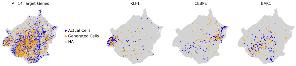
Single-node Interventional Distributions. To study the generative capacity of our model for interventions on single genes, we produce samples for each single-node intervention with over 800 cells (14 interventions). We compare these against the left-out cells of the corresponding distributions. Figure 5 illustrates this for example genes in 2 dimensions using UMAP [McInnes et al., 2018] with all other cells in the dataset as background (labeled by ‘NA’). Our model is able to discover subpopulations of the interventional distributions (e.g., for KLF1, the generated samples are concentrated in the middle left corner). We provide a quantitative evaluation for all single-node interventions in Figure 6. The model is able to obtain close to perfect (on average 0.99 over all genes and 0.95 over most differentially expressed genes).
Double-node Interventional Distributions. Next, we analyze the generalization capabilities of our model to the double-node interventions. Despite never observing any cells from these interventions during training, we obtain reasonable values (on average 0.98 over all genes and 0.88 over most differentially expressed genes). However, when looking at the generated samples for individual pairs of interventions, it is apparent that our model performs well on many pairs, but recovers different subpopulations for some pairs (examples shown in Figure 13 in Appendix G). The wrongly predicted intervention pairs could indicate that the two target genes act non-additively, which needs to be further evaluated and is of independent interest for biological research [Horlbeck et al., 2018; Norman et al., 2019].

Structure Learning. Lastly, we examine the learned DAG between the intervention targets. Specifically, this corresponds to a learned gene regulatory network between the learned programs of the target genes. For this, we reduce from until the learned latent targets of cover all latent nodes. This results in groups of genes, where genes are grouped by their learned latent nodes. We then run our algorithm with fixed multiple times and take the learned DAG with the least number of edges. This DAG over the groups of targeted genes is shown with example genes in Figure 7 (left). This learned structure is in accordance with previous findings. For example, we successfully identified the edges DUSP9MAPK1 and DUSP9ETS2, which is validated in [Norman et al., 2019] (see their Fig. 5). We also show the interventional distributions targeting these example genes in Figure 7 (right). Among these, MAPK1 and ETS2 correspond to clusters that are heavily overlapping, which explains why the model maps both distributions to the same latent node.
7 Conclusion
We derived identifiability results for causal disentanglement from single-node interventions, and presented an autoencoding variational Bayes framework to estimate the latent causal representation from interventional samples. Identification of the latent causal structure and generalization to multi-node interventions was demonstrated experimentally on genetic data.
7.1 Limitations and Future Work
This paper opens up several direction for future theoretical and empirical work, which we now discuss.
Theoretical Perspective. We have focused on the setting where a single-node intervention on each latent node is available, similar to prior works on causal disentanglement [Ahuja et al., 2022b; Squires et al., 2023]. However, we highlight three issues in this setup and discuss potential remedies. First, by assuming access to data from intervening on every single latent node, we inherently possess partial knowledge of all the latent variables, even though we are unaware of their specific values or whether multiple interventions act on the same variable. The setups that do not assume interventions but the existence of anchored observed variables (i.e., variables with only one latent parent) [Halpern et al., 2015; Cai et al., 2019; Xie et al., 2020; Xie et al., 2022] face the same issue. This assumption can be unsatisfying in the context of causal representation learning, where the causal variables are assumed to be entirely unknown. Second, it may be impossible to intervene on all latent causal variables, especially in scenarios involving latent confounding. For instance, in climate research, it might be impossible to intervene on a variable like the precipitation level in a particular region. Finally, the assumption of single-node interventions can be overly optimistic in many applications. For example, in the case of chemical perturbations on cells, it is known that drugs often target multiple variables.
Nevertheless, the results obtained in the current setup can serve as a foundation and stepping stone towards the ultimate goal of general causal representation learning. On one hand, our analysis showed what can be learned from each intervention. This is helpful when considering cases where only a subset of the latent causal variables can be intervened on. On the other hand, the key techniques employed in our proofs can be extended to the multi-node setting. Specifically, in the latent space, one should expect only the marginals of variables downstream of a multi-node intervention to change.
Moreover, we have primarily focused on the infinite data regime for analyzing identifiability. Considering the expensive nature of obtaining interventional samples in practice, there is ample room for further investigation concerning sample complexity. Aside from the feasibility of identifiability, many applications are concerned with specific downstream tasks. Full identification of the underlying causal representations provides a comprehensive understanding of the system and would be beneficial for multiple downstream tasks. However, in certain cases, full identification may be unnecessary or inefficient for a particular task. Therefore, it is of interest to develop task-specific identifiability criteria for causal representation learning.
Empirical Perspective. We make two remarks on the VAE framework proposed in this work. First, as shown in our experiments in Section 6, our proposed framework can still be applied in settings with multi-node interventions and fewer single-node interventions. For instance, one can model multi-node interventions by reducing the temperature in the softmax layer. Second, due to the permutation symmetry of CD-equivalence, we impose an upper-triangular structure on the adjacency matrix in the deep SCM and learn the intervention targets. Alternatively, when there is exactly one intervention available for each latent node, one can instead prefix the intervention targets and learn the adjacency matrix. Specifically, we can set the intervention targets of to be a random permutation of . Subsequently, the adjacency matrix can be learned for example via the nontears penalty [Zheng et al., 2018] to enforce acyclicity. However, both methods inherit the combinatorial nature of learning a DAG, and therefore their performance may require large sample sizes and can be sensitive to initialization [Kaiser and Sipos, 2021]. Consequently, endeavors to improve the optimization process and robustness of such models would be valuable.
7.2 Discussion of Contemporaneous Works.
This work is concurrent with a number of other works in interventional causal representation learning. Unless otherwise noted, all of these works consider single-node interventions, as we do in this paper. Most similar to our setting is [Varici et al., 2023], which studies identifiability of nonparametric latent SCMs under linear mixing. They consider the case where exactly one intervention per latent node is available, which is an easier setting as we discussed in Section 2. In that setting, they provide a characterization of the learned causal variables. On the other hand, Buchholz et al., 2023 studies identifiability of a linear latent SCM under nonparametric mixing. They also consider both hard and soft interventions, but in the form of linear SCM with additive Gaussian noises. Three concurrent works [Jiang and Aragam, 2023; von Kügelgen et al., 2023; Liang et al., 2023] consider both nonparametric SCMs and nonparametric mixing functions: von Kügelgen et al., 2023 prove identifiability for the case of latent variables when there is one intervention per latent variable. They provide an extension to arbitrary for settings where there are paired interventions on each latent variable. Meanwhile, [Jiang and Aragam, 2023] consider arbitrary , without paired interventions. However, they use only conditional independence statements over the observed variables to recover the latent causal graph. As a result, their identifiability guarantees place restrictions on the latent causal graph, unlike the other works discussed here. The third work [Liang et al., 2023] studies the Causal Component Analysis problem, where the latent causal graph is assumed to be known. Finally, we note that other concurrent works study causal representation learning without interventional data [Markham et al., 2023; Kong et al., 2023] or with vector-valued contexts instead of interventions [Komanduri et al., 2023].
Acknowledgements
We thank the Causal Representation Learning Workshop at Bellairs Institute for helpful discussions. All authors acknowledge support by the MIT-IBM Watson AI Lab. In addition, J. Zhang, C. Squires and C. Uhler acknowledge support by the NSF TRIPODS program (DMS-2022448), NCCIH/NIH (1DP2AT012345), ONR (N00014-22-1-2116), the United States Department of Energy (DOE), Office of Advanced Scientific Computing Research (ASCR), via the M2dt MMICC center (DE-SC0023187), the Eric and Wendy Schmidt Center at the Broad Institute, and a Simons Investigator Award.
References
- Ahuja et al., [2021] Ahuja, K., Hartford, J., and Bengio, Y. (2021). Properties from mechanisms: an equivariance perspective on identifiable representation learning. arXiv preprint arXiv:2110.15796.
- [2] Ahuja, K., Hartford, J., and Bengio, Y. (2022a). Weakly supervised representation learning with sparse perturbations. In Advances in Neural Information Processing Systems.
- [3] Ahuja, K., Wang, Y., Mahajan, D., and Bengio, Y. (2022b). Interventional causal representation learning. arXiv preprint arXiv:2209.11924.
- Arjovsky et al., [2019] Arjovsky, M., Bottou, L., Gulrajani, I., and Lopez-Paz, D. (2019). Invariant risk minimization. arXiv preprint arXiv:1907.02893.
- Arjovsky et al., [2017] Arjovsky, M., Chintala, S., and Bottou, L. (2017). Wasserstein generative adversarial networks. In International conference on machine learning, pages 214–223. PMLR.
- Brehmer et al., [2022] Brehmer, J., Haan, P. D., Lippe, P., and Cohen, T. (2022). Weakly supervised causal representation learning. In ICLR2022 Workshop on the Elements of Reasoning: Objects, Structure and Causality.
- Buchholz et al., [2023] Buchholz, S., Rajendran, G., Rosenfeld, E., Aragam, B., Schölkopf, B., and Ravikumar, P. (2023). Learning linear causal representations from interventions under general nonlinear mixing. arXiv preprint arXiv:2306.02235.
- Bunne et al., [2023] Bunne, C., Stark, S. G., Gut, G., Del Castillo, J. S., Levesque, M., Lehmann, K.-V., Pelkmans, L., Krause, A., and Rätsch, G. (2023). Learning single-cell perturbation responses using neural optimal transport. Nature Methods, pages 1–10.
- Cai et al., [2019] Cai, R., Xie, F., Glymour, C., Hao, Z., and Zhang, K. (2019). Triad constraints for learning causal structure of latent variables. Advances in neural information processing systems, 32.
- Chickering, [2002] Chickering, D. M. (2002). Optimal structure identification with greedy search. Journal of machine learning research, 3(Nov):507–554.
- Comon, [1994] Comon, P. (1994). Independent component analysis, a new concept? Signal processing, 36(3):287–314.
- Cussens, [2020] Cussens, J. (2020). Gobnilp: Learning bayesian network structure with integer programming. In International Conference on Probabilistic Graphical Models, pages 605–608. PMLR.
- Dixit et al., [2016] Dixit, A., Parnas, O., Li, B., Chen, J., Fulco, C. P., Jerby-Arnon, L., Marjanovic, N. D., Dionne, D., Burks, T., Raychowdhury, R., et al. (2016). Perturb-seq: dissecting molecular circuits with scalable single-cell rna profiling of pooled genetic screens. cell, 167(7):1853–1866.
- Fine and Rosenberger, [1997] Fine, B. and Rosenberger, G. (1997). The fundamental theorem of algebra. Springer Science & Business Media.
- Frogner et al., [2019] Frogner, C., Mirzazadeh, F., and Solomon, J. (2019). Learning embeddings into entropic wasserstein spaces. arXiv preprint arXiv:1905.03329.
- Gilbert et al., [2014] Gilbert, L. A., Horlbeck, M. A., Adamson, B., Villalta, J. E., Chen, Y., Whitehead, E. H., Guimaraes, C., Panning, B., Ploegh, H. L., Bassik, M. C., et al. (2014). Genome-scale crispr-mediated control of gene repression and activation. Cell, 159(3):647–661.
- Glymour et al., [2019] Glymour, C., Zhang, K., and Spirtes, P. (2019). Review of causal discovery methods based on graphical models. Frontiers in genetics, 10:524.
- Gretton et al., [2012] Gretton, A., Borgwardt, K. M., Rasch, M. J., Schölkopf, B., and Smola, A. (2012). A kernel two-sample test. The Journal of Machine Learning Research, 13(1):723–773.
- Halpern et al., [2015] Halpern, Y., Horng, S., and Sontag, D. (2015). Anchored discrete factor analysis. arXiv preprint arXiv:1511.03299.
- Hauser and Bühlmann, [2012] Hauser, A. and Bühlmann, P. (2012). Characterization and greedy learning of interventional markov equivalence classes of directed acyclic graphs. The Journal of Machine Learning Research, 13(1):2409–2464.
- Heinze-Deml et al., [2018] Heinze-Deml, C., Maathuis, M. H., and Meinshausen, N. (2018). Causal structure learning. Annual Review of Statistics and Its Application, 5:371–391.
- Horlbeck et al., [2018] Horlbeck, M. A., Xu, A., Wang, M., Bennett, N. K., Park, C. Y., Bogdanoff, D., Adamson, B., Chow, E. D., Kampmann, M., Peterson, T. R., et al. (2018). Mapping the genetic landscape of human cells. Cell, 174(4):953–967.
- Hyvarinen et al., [2019] Hyvarinen, A., Sasaki, H., and Turner, R. (2019). Nonlinear ICA using auxiliary variables and generalized contrastive learning. In The 22nd International Conference on Artificial Intelligence and Statistics, pages 859–868. PMLR.
- Jaber et al., [2020] Jaber, A., Kocaoglu, M., Shanmugam, K., and Bareinboim, E. (2020). Causal discovery from soft interventions with unknown targets: Characterization and learning. Advances in neural information processing systems, 33:9551–9561.
- Jiang and Aragam, [2023] Jiang, Y. and Aragam, B. (2023). Learning nonparametric latent causal graphs with unknown interventions. arXiv preprint arXiv:2306.02899.
- Kaddour et al., [2022] Kaddour, J., Lynch, A., Liu, Q., Kusner, M. J., and Silva, R. (2022). Causal machine learning: A survey and open problems. arXiv preprint arXiv:2206.15475.
- Kaiser and Sipos, [2021] Kaiser, M. and Sipos, M. (2021). Unsuitability of notears for causal graph discovery. arXiv preprint arXiv:2104.05441.
- Khemakhem et al., [2020] Khemakhem, I., Kingma, D., Monti, R., and Hyvarinen, A. (2020). Variational autoencoders and nonlinear ICA: A unifying framework. In International Conference on Artificial Intelligence and Statistics, pages 2207–2217. PMLR.
- Kingma and Welling, [2013] Kingma, D. P. and Welling, M. (2013). Auto-encoding variational bayes. arXiv preprint arXiv:1312.6114.
- Kivva et al., [2021] Kivva, B., Rajendran, G., Ravikumar, P., and Aragam, B. (2021). Learning latent causal graphs via mixture oracles. Advances in Neural Information Processing Systems, 34:18087–18101.
- Komanduri et al., [2023] Komanduri, A., Wu, Y., Chen, F., and Wu, X. (2023). Learning causally disentangled representations via the principle of independent causal mechanisms. arXiv preprint arXiv:2306.01213.
- Kong et al., [2023] Kong, L., Huang, B., Xie, F., Xing, E., Chi, Y., and Zhang, K. (2023). Identification of nonlinear latent hierarchical models. arXiv preprint arXiv:2306.07916.
- Kuipers and Moffa, [2022] Kuipers, J. and Moffa, G. (2022). The interventional bayesian gaussian equivalent score for bayesian causal inference with unknown soft interventions. arXiv preprint arXiv:2205.02602.
- Lachapelle et al., [2020] Lachapelle, S., Brouillard, P., Deleu, T., and Lacoste-Julien, S. (2020). Gradient-based neural dag learning. In International Conference on Learning Representations.
- Liang et al., [2023] Liang, W., Kekić, A., von Kügelgen, J., Buchholz, S., Besserve, M., Gresele, L., and Schölkopf, B. (2023). Causal component analysis. arXiv preprint arXiv:2305.17225.
- Lippe et al., [2022] Lippe, P., Magliacane, S., Löwe, S., Asano, Y. M., Cohen, T., and Gavves, S. (2022). Citris: Causal identifiability from temporal intervened sequences. In International Conference on Machine Learning, pages 13557–13603. PMLR.
- Liu et al., [2022] Liu, Y., Zhang, Z., Gong, D., Gong, M., Huang, B., Hengel, A. v. d., Zhang, K., and Shi, J. Q. (2022). Weight-variant latent causal models. arXiv preprint arXiv:2208.14153.
- Lorch et al., [2021] Lorch, L., Rothfuss, J., Schölkopf, B., and Krause, A. (2021). Dibs: Differentiable bayesian structure learning. Advances in Neural Information Processing Systems, 34:24111–24123.
- Lotfollahi et al., [2021] Lotfollahi, M., Susmelj, A. K., De Donno, C., Ji, Y., Ibarra, I. L., Wolf, F. A., Yakubova, N., Theis, F. J., and Lopez-Paz, D. (2021). Learning interpretable cellular responses to complex perturbations in high-throughput screens. BioRxiv, pages 2021–04.
- Markham et al., [2023] Markham, A., Liu, M., Aragam, B., and Solus, L. (2023). Neuro-causal factor analysis. arXiv preprint arXiv:2305.19802.
- McInnes et al., [2018] McInnes, L., Healy, J., and Melville, J. (2018). Umap: Uniform manifold approximation and projection for dimension reduction. arXiv preprint arXiv:1802.03426.
- Meinshausen et al., [2016] Meinshausen, N., Hauser, A., Mooij, J. M., Peters, J., Versteeg, P., and Bühlmann, P. (2016). Methods for causal inference from gene perturbation experiments and validation. Proceedings of the National Academy of Sciences, 113(27):7361–7368.
- Mooij et al., [2020] Mooij, J. M., Magliacane, S., and Claassen, T. (2020). Joint causal inference from multiple contexts. The Journal of Machine Learning Research, 21(1):3919–4026.
- Norman et al., [2019] Norman, T. M., Horlbeck, M. A., Replogle, J. M., Ge, A. Y., Xu, A., Jost, M., Gilbert, L. A., and Weissman, J. S. (2019). Exploring genetic interaction manifolds constructed from rich single-cell phenotypes. Science, 365(6455):786–793.
- Pawlowski et al., [2020] Pawlowski, N., Coelho de Castro, D., and Glocker, B. (2020). Deep structural causal models for tractable counterfactual inference. Advances in Neural Information Processing Systems, 33:857–869.
- Pearl, [2009] Pearl, J. (2009). Causality. Cambridge university press.
- Peters et al., [2017] Peters, J., Janzing, D., and Schölkopf, B. (2017). Elements of causal inference: foundations and learning algorithms. The MIT Press.
- Raskutti and Uhler, [2018] Raskutti, G. and Uhler, C. (2018). Learning directed acyclic graph models based on sparsest permutations. Stat, 7(1):e183.
- Roohani et al., [2022] Roohani, Y., Huang, K., and Leskovec, J. (2022). Gears: Predicting transcriptional outcomes of novel multi-gene perturbations. BioRxiv, pages 2022–07.
- Rothenhäusler et al., [2015] Rothenhäusler, D., Heinze, C., Peters, J., and Meinshausen, N. (2015). Backshift: Learning causal cyclic graphs from unknown shift interventions. Advances in Neural Information Processing Systems, 28.
- Sohn et al., [2015] Sohn, K., Lee, H., and Yan, X. (2015). Learning structured output representation using deep conditional generative models. Advances in neural information processing systems, 28.
- Solus et al., [2021] Solus, L., Wang, Y., and Uhler, C. (2021). Consistency guarantees for greedy permutation-based causal inference algorithms. Biometrika, 108:795–814.
- Squires et al., [2023] Squires, C., Seigal, A., Bhate, S. S., and Uhler, C. (2023). Linear causal disentanglement via interventions. In Proceedings of the 40th International Conference on Machine Learning, pages 32540–32560. PMLR.
- Squires and Uhler, [2022] Squires, C. and Uhler, C. (2022). Causal structure learning: a combinatorial perspective. Foundations of Computational Mathematics, pages 1–35.
- Stark et al., [2020] Stark, S. G., Ficek, J., Locatello, F., Bonilla, X., Chevrier, S., Singer, F., Rätsch, G., and Lehmann, K.-V. (2020). Scim: universal single-cell matching with unpaired feature sets. Bioinformatics, 36(Supplement_2):i919–i927.
- Studeny, [2006] Studeny, M. (2006). Probabilistic conditional independence structures. Springer Science & Business Media.
- Tian and Pearl, [2001] Tian, J. and Pearl, J. (2001). Causal discovery from changes. In Proceedings of the 17th Conference in Uncertainty in Artificial Intelligence, pages 512–521.
- Uhler et al., [2013] Uhler, C., Raskutti, G., Bühlmann, P., and Yu, B. (2013). Geometry of the faithfulness assumption in causal inference. The Annals of Statistics, pages 436–463.
- Varici et al., [2023] Varici, B., Acarturk, E., Shanmugam, K., Kumar, A., and Tajer, A. (2023). Score-based causal representation learning with interventions. arXiv preprint arXiv:2301.08230.
- von Kügelgen et al., [2023] von Kügelgen, J., Besserve, M., Liang, W., Gresele, L., Kekić, A., Bareinboim, E., Blei, D. M., and Schölkopf, B. (2023). Nonparametric identifiability of causal representations from unknown interventions. arXiv preprint arXiv:2306.00542.
- Vowels et al., [2022] Vowels, M. J., Camgoz, N. C., and Bowden, R. (2022). D’ya like dags? a survey on structure learning and causal discovery. ACM Computing Surveys, 55(4):1–36.
- Wang et al., [2017] Wang, Y., Solus, L., Yang, K. D., and Uhler, C. (2017). Permutation-based causal inference algorithms with interventions. In Neural Information Processing Systems, volume 31.
- Wu et al., [2019] Wu, J., Huang, Z., Acharya, D., Li, W., Thoma, J., Paudel, D. P., and Gool, L. V. (2019). Sliced wasserstein generative models. In Proceedings of the IEEE/CVF Conference on Computer Vision and Pattern Recognition, pages 3713–3722.
- Xie et al., [2020] Xie, F., Cai, R., Huang, B., Glymour, C., Hao, Z., and Zhang, K. (2020). Generalized independent noise condition for estimating latent variable causal graphs. Advances in neural information processing systems, 33:14891–14902.
- Xie et al., [2022] Xie, F., Huang, B., Chen, Z., He, Y., Geng, Z., and Zhang, K. (2022). Identification of linear non-gaussian latent hierarchical structure. In International Conference on Machine Learning, pages 24370–24387. PMLR.
- [66] Yang, K., Katcoff, A., and Uhler, C. (2018a). Characterizing and learning equivalence classes of causal dags under interventions. In International Conference on Machine Learning, pages 5541–5550. PMLR.
- [67] Yang, K. D., Katcoff, A., and Uhler, C. (2018b). Characterizing and learning equivalence classes of causal DAGs under interventions. Proceedings of Machine Learning Research, 80:5537–5546.
- Yu and Welch, [2022] Yu, H. and Welch, J. D. (2022). Perturbnet predicts single-cell responses to unseen chemical and genetic perturbations. BioRxiv, pages 2022–07.
- Zhang et al., [2021] Zhang, J., Squires, C., and Uhler, C. (2021). Matching a desired causal state via shift interventions. Advances in Neural Information Processing Systems, 34:19923–19934.
- Zheng et al., [2018] Zheng, X., Aragam, B., Ravikumar, P. K., and Xing, E. P. (2018). Dags with no tears: Continuous optimization for structure learning. Advances in Neural Information Processing Systems, 31.
- Zimmermann et al., [2021] Zimmermann, R. S., Sharma, Y., Schneider, S., Bethge, M., and Brendel, W. (2021). Contrastive learning inverts the data generating process. In International Conference on Machine Learning, pages 12979–12990. PMLR.
Appendix A Useful Lemmas
A.1 Remarks on Assumption 1
Here we show that the assumption on the functional class of is satisfied if is linear and injective, whenever the support of has non-empty interior. Recall Assumption 1. See 1
Denote the support of as respectively. Let be the interior of .
Lemma 2.
Suppose is a non-empty subset of . If is linear and injective, then it must be a full row rank polynomial.
Proof.
Since is linear, it can be written as for some and . If is not of full row rank, then there exists a non-zero vector such that . Let , then there exists such that . We have , which violates being injective. Therefore must have full row rank. ∎
A.2 Proof of Lemma 1
The proof of Lemma 1 follows from [Ahuja et al., 2022b]. For completeness, we present a concise proof here. Then we state a few remarks. Recall Lemma 1. See 1
Proof.
We solve for the smallest integer such that there exists a full row rank polynomial where for has non-empty support . In other words, denote all pairs of that satisfy Assumption 1 as , we solve for
| (4) |
Note that for all . Since are full row rank polynomials, there exist full row rank matrices and vectors such that
| (5) |
Since are of full rank, they have pseudo-inverses such that and . Multiplying to Eq. (5), we have
Therefore can be written as a polynomial of , i.e., . Similarly, we have . Therefore for all . Since is non-empty, we know that on some open set. By the fundamental theorem of algebra [Fine and Rosenberger, 1997], we know that and must have degree . Thus for some full row rank matrix and vector . Since is of full row rank, it indicates that . Since satisfy , by Eq. (4), we must have . Thus and for some non-singular matrix and vector .
This proof also shows that we can only identify up to such linear transformations with observational data. Since for any non-singular matrix and vector , let . We have satisfy Assumption 1 and they generate the same observational data. ∎
Remark 1.
With observational data , we can identify such that for non-singular . Then for any interventional data , the analytic continuation of to satisfies for all .
Proof.
The proof follows immediately by writing as polynomial functions. ∎
Next, we discuss identifiability of the underlying DAG . First, we give an example showing that any causal DAG can explain the observational data.
Example 4.
Suppose the ground-truth DAG is an empty graph . With observational data alone, any DAG can explain the data.
Proof.
Let be an arbitrary DAG with topological order , i.e., only if . Let be the permutation matrix such that satisfies for any . Then factorizes as . This implies for . Therefore and factorizes with respect to . Thus can explain the data. ∎
Therefore with observational data alone, we cannot identify the underlying DAG up to any nontrivial equivalence class. In [Ahuja et al., 2022b], it was shown that with a do intervention66 6 Do interventions are a special type of hard interventions where the intervention target collapses to one specific value. per latent node and assuming the interior of the support of the non-targeted variables is non-empty, one can identify up to a finer class of linear transformations. Namely, one can identify up to CD-equivalence (permutation and element-wise affine transformation); see Definition 1. Then, assuming for example faithfulness and influentiality [Tian and Pearl, 2001], one can identify .
While several extensions beyond do-interventions are discussed in [Ahuja et al., 2022b], they all involve manipulating the support of the intervention targets. In the case where the support of the intervention targets remains unchanged (e.g., additive Gaussian SCMs with shift interventions), a completely new approach and theory needs to be developed.
Appendix B Proof of Identifiability with Soft Interventions
In this section, we provide the proofs for the results in Section 4. While our main focus is on general types of soft interventions, our results also apply to hard interventions which include do-interventions as a special case.
Notation. We let denote the indicator vector with the -th entry equal to one and all other entries equal to zero. To be consistent with other notation in the paper, let be a row vector. We call a maximal child of if . Denote the set of all maximal children of as . For node , define . Given a DAG , we denote the transitive closure of by , i.e., if and only if there is a directed path from to in .
B.1 Faithfulness Assumptions
We start by discussing previous interventional faithfulness assumptions. Prior interventional faithfulness assumptions [Tian and Pearl, 2001; Yang et al., 2018a; Jaber et al., 2020] vary by a few technicalities; but they all assume that all causal variables are observed (causal sufficiency), and, more importantly, that intervening on a node will always change the marginal of its descendants. In particular, [Tian and Pearl, 2001] (Definition 2, called “influentiality”) only made this assumption and showed that the causal graph is identifiable up to its transitive closure by detecting marginal changes. [Tian and Pearl, 2001] showed that their algorithm consistently identifies the full causal graph by assuming additionally that intervening on a node changes the conditional distribution of its direct children giving its neighbors (details can be found in Assumption 4.5 of [Yang et al., 2018a]). A similar notion was also introduced in [Jaber et al., 2020] where they made further assumptions regarding changes in the conditional distributions.
We now show our linear interventional faithfulness (Assumption 2) is satisfied by a large class of nonlinear SCMs and soft interventions. Recall Assumption 2. See 2
In Example 2, we discussed a -node graph where Assumption 2 is satisfied. This example can be extended in the following way, which subsumes the case in Example 3.
Example 5.
Consider an SCM with additive noise, where each mechanism is specified by , where for are independent exogenous noise variables. Assumption 2 is satisfied if only changes the variance of and is a quadratic function with non-zero coefficient of for each .
Proof.
If in Assumption 2, then . Since , we have
Note that does not change the joint distribution of , and therefore
By , we then know that. Thus .
If in Assumption 2, then by linearity of expectation . Note that , and therefore . Next we show that . Once this is proven, then we have that , which concludes the proof for .
Since is a quadratic function of , suppose the coefficient of in is . Then
| (6) | ||||
for some functions and . Since , we know that will not change the joint distribution of and that . Therefore we have
By , and Eq. (6), we have , which concludes the proof. ∎
This example shows how we may check by examining the mean and variance of . In general, this can be extended to checking any finite moments of as stated in the following lemma.
Lemma 3.
Assumption 2 is satisfied if for each one of the following conditions holds:
- (1)
if , then there exits an integer such that
and the smallest that satisfies this also satisfies . In addition, for all , it holds that ;
- (2)
if , then for all , there exists an integer such that
where is as defined in Assumption 2, and the smallest that satisfies this also satisfies , where
Proof.
Suppose (1) holds true. If in Assumption 2, then for , and
where the inequality is because of and for any . Therefore .
If in Assumption 2, then implies , which proves that .
Suppose (2) holds true. If in Assumption 2, then implies , which proves that .
If in Assumption 2, then for , if the coordinate for is not , then , since . If the coordinate for in is , denote , and then similar to above we obtain
Thus , which completes the proof. ∎
This lemma gives a sufficient condition for Assumption 2 to hold. Since it involves only finite moments of the variables, one can easily check if this is satisfied for a given SCM associated with soft interventions. Note that Example 5 satisfies the first condition of Lemma 3 for .
Next we show that Assumption 3 is satisfied on a tree graph if Assumption 2 holds, under mild regularity conditions such as that the interventional support lies within the observational support. Recall Assumption 3.
See 3
Lemma 4.
Proof.
Suppose is a tree graph and Assumption 2 holds for targeting . For any edge , since there is only one undirected path between and , we have . Therefore we only need to show that and are not conditionally independent given for any .
Suppose and are conditionally independent given . Then for any and realization of (denote the realization of as ),
Since this is true for any with , by Eq. (8), we have
Note that since targets , and we therefore have
where the second-to-last equality uses the regularity condition in Eq. (7).
Since , it holds that , and thus , which is a contradiction to linear interventional faithfulness of . Therefore, we must have that and are not conditionally independent given , which completes the proof. ∎
Essentially, Assumption 2 guarantees influentiality and Assumption 3 guarantees adjacency faithfulness. These assumptions differ from existing faithfulness conditions (c.f., [Tian and Pearl, 2001; Uhler et al., 2013; Yang et al., 2018b]) due to the fact that we can only observe a linear mixing of the causal variables.
B.2 Summary of representations
In the remainder of this appendix, we will develop a series of representations which are increasingly related to the underlying representation . These representations are summarized in Table 1.
B.3 Proof of Theorem 1
In the main text (Section 4.2), we laid out an illustrative procedure to identify the transitive closure of when we consider a simpler setting with . This process relies on iteratively finding source nodes of . In the generalized setting with , the proof works in the reversed way, where we iteratively identify the sink nodes88 8 A sink node is a node without children of .
In Section B.3.1, we introduce the concept of a topological representation: a representation of the data for which marginal distributions change in a way consistent with an assignment of intervention targets. In Lemma 5, we show that under Assumptions 1 and 2, a topological representation is guaranteed to exist. In Lemma 6, we show that any topological representation is also topologically consistent in a natural way with the underlying representation .
In Section B.3.2, we consider transforming a topological representation into a different topological representation . For any such representation , we define an associated graph . In Lemma 7, we show that picking so that has the fewest edges will yield that .
Together, these results are used to prove Theorem 1: that we can identify up to transitive closure.
B.3.1 Topologically ordered representations
We begin by introducing the concept of a topological representation.
Definition 2.
Suppose . Let be a non-singular matrix, let , and let . We call a topological representation of with intervention targets if the following two conditions are satisfied for all :
-
(Condition 1) .
-
(Condition 2) and for any .
Here, are the induced distributions for when and , respectively.
The next result shows that a topological representation always exists. In particular, we show that a topological representation can be recovered simply be re-ordering the nodes of .
Lemma 5.
Suppose that Assumption 2 hold. Then, there exists a topological representation of .
Proof.
Assume without loss of generality that has topological order , i.e., only if . Let , then for constant vector . Set to be such that for . Let and .
Condition 1. Since targets , by Assumption 2, we have , and thus .
Condition 2. Since targets and , we have , and thus . ∎
Now, we show that any topological representation is also consistent with the underlying representation up to some linear transformation which respects the topological ordering.
Lemma 6.
Suppose that Assumptions 2 hold. Let be a topological representation of and denote . Then, there exists a topological ordering of such that for any , we have that
| (9) |
Proof.
We prove by induction. Let . Note that .
Base case.
Consider .
Let .
We will show that must be a sink node in .
Suppose is not a sink node, and let . Since is nonsingular, . Therefore, we must have . Thus,
By Condition 2, we have that . Since is a constant, this implies that . However, this contradicts Assumption 2. Thus, must be a sink node, which we denote by .
We also have that for any . Otherwise suppose , then can be written as with . By Assumption 2, we have , a contradiction to Condition 2.
Induction step.
Suppose that we have proven the statement for .
Denote the intervention targets of as , respectively.
Let .
Consider with . Let denote the graph after removing the nodes . We will show that must be a sink node in .
Suppose that is not a sink node and let be a maximal child of in . Since , , and is nonsingular, we have that is nonsingular. Thus, as above,
where are indicator vectors in with ones at positions of in after removing , respectively. Thus, by Condition 2, we have that , which contradicts Assumption 2. Therefore targets a sink node of .
To show that for any , use for all and write as with . By Assumption 2, we have if , a contradiction to Condition 2.
By induction, we have thus proven that the solution to Condition 1 and Condition 2 satisfies . Therefore is upper triangular. Since it is also non-singular, it must hold that . Thus Eq. (9) holds for some unknown . Furthermore, the proof shows that target respectively. ∎
B.3.2 Sparsest topological representation
In the section, we will introduce a graph associated to any topological representation. We consider picking a topological representation such that the associated graph is as sparse is possible, and we show that this choice recovers the underlying graph up to transitive closure.
We begin by establishing the following property of a topological representation , which relates ancestral relationships in the underlying graph to changes in marginals of .
Proposition 1.
Suppose that Assumptions 2 hold. Let be a topological representation with intervention targets .
Then, for any such that , we must have
Proof.
By Lemma 6, Eq. (9), is a linear combination of with nonzero coefficient of . Let be
- (Case 1)
the largest such that where and the coefficient of in is nonzero,
- (Case 2)
, if no satisfies Case 1.
Then let if ; otherwise let be such that and (such exists by considering the parent of on the longest directed path from to in ). Figure 8 illustrates the different scenarios for . Note that we always have .


(Case 1): We first show that can be written as a linear combination of and for with nonzero coefficient for . Consider an arbitrary . If the coefficient for in is nonzero, by Eq. (9), we have . Also since is the largest, we have or or or . If , then by the topological order, it holds that . If , since , it also holds that . Therefore can be written as a linear combination of and with nonzero coefficient for . Next, we show that by considering two subcases of Case 1.
If , then (illustrated in Figure 8A). Then . Therefore can be written as a linear combination of and for with nonzero coefficient for . By Assumption 2, we have .
If , then since , we have (illustrated in Figure 8B). Then we have , and thus . In fact, is a subset of , since by (definition of ). Therefore can be written as a linear combination of and for with nonzero coefficient for . Since (definition of ), by Assumption 2, we have , as targets .
(Case 2): In this case (illustrated in Figure 8C). Then for any such that , the coefficient of in is zero. Otherwise since , it holds that , which by Eq. (11) implies . Thus satisfies Case 1, a contradiction. Therefore, also by Eq. (11), can be written as a linear combination of and with nonzero coefficient of , where .
Since , by definition of , we have . Note that can be written as a linear combination of and with nonzero coefficient of , where . By Assumption 2, , as targets .
Therefore, in both cases it holds that . Since and , the claim is proven. ∎
Now, we use marginal changes to define a graph associated to any topologically-ordered representation. We use Proposition 1 to show that picking the the topologically-ordered representation which yields the sparsest graph will recover the transitive closure of .
Lemma 7.
Let be a topological representation of with intervention targets . Let be an invertible upper triangular and let . Define the following:
- •
Let be the DAG such that if and only if and .
- •
Let .
Let be such that has the fewest edges over any choice of . Then . We call a sparsest topological representation of .
Proof.
Direction 1.
We first show that for any ,
| (10) |
Let , so . By Proposition 1, we have such that with . By definition of , we have . Repeating this argument iteratively, we obtain a directed path from to in . Thus, by definition of , we have .
Direction 2.
Now we give an example of such that the constructed satisfies
Denote and . Since is upper-triangular and invertible, by Eq. (9), we have , where
| (11) |
where is the topological order in Eq. (9). By Eq. (11), there exists an invertible upper-triangular matrix such that for some constant vector . Now for , we have . Since targets , this would only be true when . Therefore . Thus . As is a transitive closure, this means . ∎
Analogously to Lemma 6, the following result shows that a sparsest topological representation is topologically consistent with in a stronger sense than a topological representation.
Lemma 8.
Let Assumption 2 hold. For and , let be a sparsest topological representation of with intervention targets . Let be a topological ordering of such that
| (12) |
Then for .
Proof.
For sake of contradiction, let . Without loss of generality, let be the largest value for which and . By transitivity of and the choice of as the largest value, there is no such that and . Therefore can be written as a linear combination of and with nonzero coefficient of , where .
By Assumption 2, we have . Since and , we have , in which case violates Condition 1, a contradiction. ∎
B.3.3 Proof of Theorem 1
See 1
Here, we combine the results of the previous two sections to show that we can recover up to transitive closure and permutation, and that we recover the intervention targets up to the same permutation.
Proof.
By Lemma 1 and Remark 1, we can assume, without loss of generality, that is known and that for some non-singular matrix , as this can be identified from observational data .
By Lemma 7, we can identify a topological representation with intervention targets , where and . Further, for some unknown topological ordering of , satisfies Eq. (11), for , and we identify .
Identifying additional intervention targets.
So far, we only guarantee that we identify the intervention targets for .
Now, consider any .
Let be such that .
We now argue that can be identified as the smallest in such that .
By Assumption 2, we have , since targets and can be written as a linear combination of with nonzero coefficient (note that ).
On the other hand, for , we have , since can be written as a linear combination of and is the topological order. ∎
B.4 Proof of Theorem 2
In this section, we show that by introducing Assumption 3, we can go beyond recovering the transitive closure of , and we instead recover . We begin by establishing a basic fact about conditional independences in our setup.
Claim 1.
Under Assumption 1, let denote (potentially linear combinations of) components of , and assume that and . Then .
Proof.
By Assumption 1, has positive measure on some full-dimensional set. By Proposition 2.1 of [Studeny, 2006], is a graphoid, i.e., it obeys the intersection property. Invoking this property, we obtain , as desired. ∎
Note that, from Theorem 1, we have already identified the interventions up to CD-equivalence for a permutation . Thus, the only remaining result to show is that we identify up to the same permutation.
In particular, we can again characterize the solution in terms of the sparsest solution.
Theorem 2, Constructive.
Let be a sparsest topological representation of with intervention targets . Let be an invertible upper triangular matrix, and let . Define the following:
- •
Let be the DAG such that for , if and only if
Let be such that has the fewest edges over any choice of . Then for satisfying Eq. (12).
Proof.
By Lemma 7, we have for some matrix satisfying Eq. (9) under some topological order of . Further, we identify .
Denoting and , by Lemma 8, we have with
| (13) | ||||
Direction 1.
First, we show that
Assume on the contrary that there exists such that . By definition, we have . By Eq. (13), we know that we can retrieve by linearly transforming ; this implies . By subtracting terms in from and then subtracting terms from for , we have that
| (14) | ||||
for some . Since by Eq. (13) there is for any , this subtraction gives us if .
Therefore let
where . There is .
On the other hand, since , i.e., . We will now show that this implies . Starting with the local Markov property, we have for any that
| (15) | ||||
where the first implication follows from the definition of conditional independence, and the second implication follows since is a deterministic function of .
Thus, by Claim 1, if and , then , i.e.,
Since for any and is the topological order, this can be further written as
where , which violates Assumption 3. Therefore we must have .
Direction 2.
There exists an invertible upper-triangular matrix such that for some constant vector .
Note that clearly satisfies Condition 1.
Also for such that , by the Markov property and being the topological order, we have .
Thus , and hence , which completes the proof.
∎
Remark 2.
These proofs (Lemma 1, Theorem 1,2) together indicate that under Assumptions 1,2,3, we can identify up to its CD-equivalence class by solving for the smallest , an encoder , and that satisfy
- (1)
there exists a full row rank polynomial decoder such that for all ;
- (2)
the induced distribution on by factorizes with respect to ;
- (3)
the induced distribution on by where changes the distribution of but does not change the joint distribution of non-descendants of in ;
- (4)
;
- (5)
has topological order ;
- (6)
the transitive closure of the DAG is the sparsest amongst all solutions that satisfy (1)-(5);
- (7)
the DAG is the sparsest amongst all solutions that satisfy (1)-(6);
We will use these observations in Appendix E to develop a discrepancy-based VAE and show that it is consistent in the limit of infinite data.
Proof.
We first show that there is a solution to (1)-(7). For this, it suffices to show that there is a solution to (1)-(5). Then since and are discrete, one can find the solution to (1)-(7) by searching amongst all solutions to (1)-(5) such that is the smallest and (6)-(7) are satisfied. Assume without loss of generality that has topological order . Then , , , and for satisfy (1)-(5).
Next we show that any solution must recover and that is in the same CD equivalence class as . Since we solve for the smallest , the former paragraph also implies that . By the proof of Lemma 1, (1) guarantees that . Therefore it must hold that .
Since we solve for the sparsest transitive closure, the first paragraph implies that . Also by the proof of Lemma 1, can be written as an invertible linear mixing of . Then (3)-(5) guarantee that Condition 1 and Condition 2 in Step 1 in the proof of Theorem 1 are satisfied. Then by the proof of Step 2 in the proof of Theorem 1, we have . Therefore, it must hold that .
Lastly, by (2) and (5), we obtain that satisfies Condition 1 and Condition 2 in Theorem 2. Therefore by the proof of Theorem 2, we obtain . Again, by the first paragraph and the fact that the sparsest transitive closure satisfies , we obtain that the sparsest with this transitive closure must satisfy , and thus . With this result, it is easy to see that for all , as changes the distribution of but does not change the joint distribution of .
Therefore we can recover and the CD equivalence class of by solving (1)-(7). Note that this proof assumes the topological order of is , and therefore it does not violate the fact that cannot be recovered exactly. ∎
B.5 Proof of Theorem 3
Now, we will show that recovering up to Theorem 1 is sufficient for predicting the effect of combinatorial interventions..
Theorem 3.
Proof.
Since contains interventions with different intervention targets, for each , we can define as if for some and otherwise . Using this definition, we define the joint distribution of as . In the following we show that in the sense that for all .
Our proof combines the following equalities. For any , we have
-
Equality 1: ,
-
Equality 2: ,
-
Equality 3: .
Proof of Equality 1. This follows by definition of , since it is transitively closed, we have .
Proof of Equality 2. By similar arguments below Eq. (13), we have for an invertible matrix , where for any . Therefore we can recover by linear transforming and vise versa. We can also recover by subtracting linear terms of from .
Note also, since , there must be . Thus
Proof of Equality 3. Follows from the Markov property on .
Combining these equalities, we have for all . Thus . Therefore the procedure in Section 4.4 generates from the same distribution as . ∎
Appendix C Details on Discrepancy-based VAE
In previous sections, we have shown that the data-generating process in Section 2 is identifiable up to equivalence classes. However, the proofs (Appendix A, B) do not lend themselves to an algorithmically efficient approach to learning the latent causal variables from data. Therefore, we propose a discrepancy-based VAE in Section 5, which inherits scalable tools of VAEs that can in principle learn flexible deep latent-variable models. In this framework, Eq. (3) can be computed and optimized efficiently using the reparametrization trick [Kingma and Welling, 2013] and gradient-based optimizers.
C.1 Maximum Mean Discrepancy
We recall the definition of the maximum mean discrepancy measure between two distributions, and its empirical counterpart.
Definition 3.
Let be a positive definite kernel function and let be the reproducing kernel Hilbert space defined by this kernel. Given distributions and , we define
The following empirical counterpart is an unbiased estimate of the squared MMD, see Lemma 6 of [Gretton et al., 2012].
Definition 4.
Let be a positive definite kernel. Let be samples from and be samples from . We define
C.2 Discrepancy VAE Details
We walk through the details of this model in this section, where we illustrate it using two types of interventions, namely do interventions and shift interventions.
Noiseless vs. Noisy Measurement Model with General SCMs. Recall that each latent causal variable is a function of its parents in and an exogenous noise term . All the ’s are mutually independent. The overall model can be defined (recursively) as
| (16) | ||||
In particular, there exists a function such that . We model each intervention as a set of intervention targets and a vector . Under , the observations are generated by
| (17) | ||||
As above, there exists a function such that . Note that here we assume that the measurements (sometimes called ‘‘observations’’ in the literature99 9 We use “measurements” to distinguish from the observational distribution defined for .) are noiseless. Our theoretical results are built upon noiseless measurements. In practice, however, one can consider the noisy measurement model in which (resp. ), where is some measurement noise independent of .
We leave as future work to prove consistency under the noisy measurement model. [Khemakhem et al., 2020] established identifiability results of the noisy measurement model, when the latent variables conditioned on additionally observed variables follow a factorized distribution in an exponential family. Their techniques can be potentially used to generalize our results to the noisy measurement model; however, further assumptions on the mechanisms ’s will be needed.
Discrepancy-based VAE. We use one decoder
parameterized by to approximate both and in the noiseless measurement model (or and in the noisy measurement model). As for the encoder, we do not directly learn the posteriors and . Instead, we approximate one posterior and then use Eq. (16), (17) to transform into , respectively. This is done by two encoders for and parameterized by and denoted as
The dimension of is set as a hyperparameter. Note that the procedure of learning a posterior in the observational distribution and then mapping to using Eq. (17) can be regarded as learning the counterfactual posterior of .
In the following, to better distinguish data from observational and interventional distributions, we use instead of to denote samples generated by Eq. (16). After encoding and into and respectively, we parameterize the causal mechanisms ’s in Eq. (16), (17) as neural networks (e.g., multi-layer perceptrons or linear layers). We absorb the paramterizations of ’s into and denote
Note that in implementation, to make sure only depends on its parents , one can train an adjacency matrix that is upper-triangular up to permutations and then apply any layers after individual rows of matrix 1010 10 Here denotes the Kronecker product.. Since identifiability can be only up to permutations of latent nodes, one can simply use an upper-triangular adjacency matrix .
Appendix D Lower Bound to Paired Log-Likelihood
In this section, we consider the paired setting, in which we have access to samples from the joint distribution . To discuss counterfactual pairs, we must introduce structure beyond the structure described in Section 2. In particular, in the observational setting, assume that the latent variables are generated from a structural causal model with exogenous noise terms . This implies that there is a function such that . Similarly, under intervention , assume there is a function such that . Then, given a distribution , the joint distribution is simply the induced distribution under the maps and .
Since and are independent conditioned on , we have
| (18) | |||
We have the following result on the loss function in Eq. (3).
Proposition 2.
Let be a Gaussian kernel with width , i.e., . Let be Gaussian with mean and a fixed variance . Then, for sufficiently large, for given in the proof, and for some constant depending only on and data dimension ,
Thus, up to an additive constant, lower bounds the paired-data ELBO in Eq.(18) and by extension the paired-data log-likelihood .
Proof.
By the choice of a Gaussian distribution for , we have
| (19) |
where is a constant depending only on and data dimension . Let be independent and identically distributed according to . Then
Now, for the empirical MMD, we have
where we have used the positivity of the exponential function and for the penultimate inequality used the fact that is large enough and that for sufficiently small. Substituting into (D) yields the theorem, with . ∎
Appendix E Consistency of Discrepancy-based VAE
We consider Discrepancy-based VAE described in the last section. Suppose the conditions in Theorem 2 is satisfied by the ground-truth model, i.e., it is possible to identify CD-equivalence class in theory.
E.1 CD-Equivalence Class
Theorem 4.
Let , , , be generated as in Section 2. Suppose that Assumptions 1, 2, and 3 hold. Define
for defined in Equation 3. Further, suppose that the VAE prior is equal to the true distribution over , that and are Dirac distributions. Let be the solution induced by .
Then is CD-equivalent to .
Proof.
Note that the parameterization of , , and the induced distributions of through prior using Eq. (16), (17) satisfy (2),(3) and (5) in Remark 2.
The first two terms in combined in Eq. (18) satisfy
where the equality holds if and only if and . On the other hand, since is a valid measure between distributions, we have
where the inequality is satisfied with equality if and only if and are equal in distribution.
Therefore if the learned intervention targets of cover and the minimum loss function is not larger that for , we have the solution satisfy (1)-(5) in Remark 2. Since has the sparsest transitive closure and is the sparsest with this transitive closure, (6)-(7) in Remark 2 are also satisfied. Therefore Remark 2 guarantees the smallest satisfying the conditions recovers the CD-equivalence class. ∎
Note that in practice, it can be hard to ensure that the gradient-based approach returns a DAG that has the sparsest transitive closure and is simultaneously the sparsest DAG with this transitive closure. We instead search for sparser DAGs by penalizing its corresponding adjacency in Eq. (3).
E.2 Consistency for Multi-Node Interventions
Theorem 3 guarantees that in an SCM with additive noises where interventions modify the exogenous noises, if the CD equivalence can be identified, we can extrapolate to unseen combinations of interventions with different intervention targets. In fact, for certain types of interventions, extrapolation to unseen combinations of any interventions is possible. We illustrate this for shift interventions in an SCM with additive Gaussian noises, where an intervention changes the mean of the exogenous noise variable.
For single-node intervention , let denote the corresponding changes in the mean of the exogenous noise variables, i.e.,
We encode it as with containing one element and being a one-hot vector, where
We extend this notation for with potentially multiple intervention targets (i.e., sets that contain multiple elements) where can be a multi-hot vector.
In the shift intervention case, from Theorem 3, we know that the encoded satisfy in the limit of infinite data, where is a linear operation with . Thus for single-node interventions amongst , the multi-node intervention 1111 11 Note that we allow overlapping intervention targets among , where adds up all the shift values for intervention target . corresponds multi-hot vector that satisfies . Thus if we encode as , we can also generate from the ground-truth distribution of where following the encoding-decoding process of Fig. 4.
Appendix F Discrepancy-based VAE Implementation Details
We summarize our hyperparameters in Table 2. Below, we describe where they are used in more detail. We use a linear structural equation with shift interventions. In practice, due to the nonlinear encoding from the latent to observed , not much expressive power is lost. Code for our method is at https://github.com/uhlerlab/discrepancy_vae.
| Loss function | |
| Kernel width (MMD) | 200 |
| Number of kernels (MMD) | 10 |
| 0.1 | |
| 1 | |
| 1 | |
| Training | |
| 100 | |
| Learning rate | 0.001 |
| Batch size | 32 |
VAE Parameterization. As is standard with VAEs, our encoder and decoder are parameterized as neural networks, and the exogenous variables are described via the reparameterization trick. We use a standard isotropic normal prior for . To encode interventions, the function is parameterized as a fully connected neural network, where for differentiable training is encoded as a one-hot vector via a softmax function, i.e., for some fully connected and temperature . During training, we adopt an annealing temperature for . In particular, until half of the epochs elapse, and is linearly increased to over the remaining epochs. At test time, the temperature of the softmax is set to a large value, recovering a close-to-true one-hot encoding.
Loss Functions. We use a mixture of MMD discrepancies, each with a Gaussian kernel with widths that are dyadically spaced [Gretton et al., 2012]. This helps prevent numerical issues and vanishing gradient issues in training. The coefficient of the discrepancy loss term is given the following schedule: for the first 5 epochs, then is linearly increased to until half of the epochs elapse, at which point it remains at for the rest of training. Similarly, the coefficient of the KL regularization term is given the following schedule: for the first 10 epochs, then is linearly increased to until half of the epochs elapse, at which point it remains at for the rest of training.
Optimization. We train using the Adam optimizer, with the default parameters from PyTorch and a learning rate of .
Biological Data. For the experiments described in Section 6, the encoder was implemented as a 2-layer fully connected network with leaky ReLU activations and 128 hidden units. The intervention encoder uses 128 hidden units. To account for interventions with less samples, we use a batch size of . We train for epochs in total, which takes less than minutes on a single GPU.
Appendix G Extended Results on Biological Dataset
In this section, we provide additional evaluations of the experiments on the Perturb-seq dataset. The computation of RMSE are computed for individual interventional distributions. The computation of (we capped the minimum by to avoid overflow) records the coefficient of determination by regressing the mean of the generated samples on the ground-truth distribution mean.
G.1 Single-node interventions
Figure 9 shows the same visualization as Figure 5 in the main text for the remaining single target-gene interventions with more than cells. Figure 10 presents this side-by-side for the training samples. For the entire single interventions, we visualize for each individual intervention the empirical MMD between the generated populations and ground-truth populations in Figure 11, where the bars record the MMD in different batches.


G.2 Double-node interventions
We plot the generated samples for 11 random double target-gene interventions in Figure 12. In Figure 13, we highlight two interventions for which the generated samples differ from the actual samples. The plots for all interventions are provided at https://github.com/uhlerlab/discrepancy_vae.

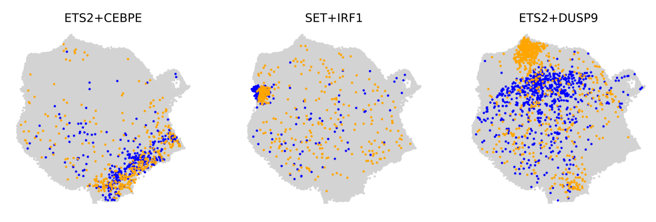
The MMD losses for all 112 interventions are summarized in Figure 14. Similar to Figure 6 in the main text, Figure 15 shows the distribution of RMSE and of the 112 interventions.
We remark here that this task has also been studied in previous works (e.g., [Lotfollahi et al., 2021; Bunne et al., 2023; Yu and Welch, 2022; Roohani et al., 2022]) with different setups. Formally benchmarking the empirical results under a unified setting would be of interest in future works.
G.3 Structure Learning
In Figure 16, we show the learned latent structure between gene programs, along with descriptions of each gene program.
Appendix H Extended Experiments
In this section, we provide additional experimental results. First, we perform ablation studies of different components of the proposed architecture on biological data. Then, we provide a simple simulation study to examine the performance of the framework on different tasks.
H.1 Ablation Studies
For the ablation studies of different components, we compared the performance of our final model (depicted in Figure 4) against three alternative versions. All models are trained with the same setting (data split, schedule, learning rate, etc). In particular, we compared against
- •
Models without the discrepancy loss. These models learn the distributions similar to conditional VAE [Sohn et al., 2015], where both an interventional sample and its interventional label are fed in to learn the exogenous . Then inside the latent space, we use the same causal layer as our model to generate a virtual sample. During inference, we can generate interventional samples via two approaches. One is sampling the exogenous from and decoding. The other is sampling an observational sample, obtaining its exogenous using the encoder then decoding. These two approaches correspond to the second and third rows of Table 3 respectively.
- •
We note that the encoder, decoder, DSCM, and intervention encoder are needed to learn distributions and the latent causal graph from this setting where observational and interventional data are present.
For the metrics, we report both MMD and in Table 3. However, MMD is more meaningful as we are assessing the quality of generating a distribution. We observe that models without discrepancy perform much worse due to mode collapses, whereas the sampling approach using observational data performs slightly better. Our final model works the best in general; however on the MMD for double-node interventions, the version without a causal layer seems to work slightly better. This is potentially because some double-node interventions that act non-additively can be captured better without imposing the structure.
| Method | MMD (single) | (single) | MMD (double) | (double) |
|---|---|---|---|---|
| ours | 0.3240.007 | 0.9860.001 | 0.4320.006 | 0.9780.001 |
| ours w/o discrepancy | 2.9660.054 | 0.9840.003 | 3.3580.031 | 0.9720.002 |
| ours w/o discrepancy (obs) | 2.9650.054 | 0.9840.002 | 3.3550.030 | 0.9720.002 |
| ours w/o causal layer | 0.3480.009 | 0.9820.002 | 0.4270.006 | 0.9780.002 |
H.2 Simulation
For the simulation study, as a proof-of-concept, we tested on a simple -node graph, where we generate samples in each of the interventional datasets. We map this to a -dimensional observation space, where we pad zeros to the additional dimensions. This ensures clear visualization of the generated samples in Figure 17, where we compare the zero-shot learned double-node interventional samples against ground truth. In Table 4, we report the quantitative metrics. In addition to the MMD on left-out single and double-node interventions, we also report the training MMD and Structural Hamming Distance (SHD) of the learned graph.
Due to the combinatorial nature of learning a DAG and the small sample sizes in this setting, we observe that the learned intervention targets can be quite sensitive to initializations. Therefore during evaluation, we report the metrics while fixing the intervention targets to be of different transposition distances to the true targets. For single-node generations, different transposition distances return similar results, meaning that the model is expressive enough to learn these distributions, although we observe that the result with zero transposition distance is marginally better. This also holds during training, which can potentially be used as model selection to overcome the initialization issue. For double-node extrapolation, the result with zero transposition distance shows a larger benefit, as expected from our theory.
| Transposition Distance | MMD (training) | MMD (single) | MMD (double) | SHD |
|---|---|---|---|---|
| 0 | 0.0300.007 | 0.0470.008 | 0.0410.004 | 2 |
| 1 | 0.0570.028 | 0.0580.030 | 0.1810.048 | 6 |
| 10 | 0.0420.007 | 0.0410.009 | 0.1190.023 | 11 |
