Combining DVL-INS and Laser-based Loop Closures in a Batch Estimation Framework for Underwater Positioning

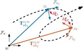
A planar reference frame ${\mathcal{F}_{a}}$ is composed of two orthonormal physical basis vectors. The planar position of physical point $\color[rgb]{0,0,0}{z}\color[rgb]{0,0,0}$ relative to physical point $\color[rgb]{0,0,0}{w}\color[rgb]{0,0,0}$, resolved in reference frame ${\mathcal{F}_{\color[rgb]{0,0,0}{a}\color[rgb]{0,0,0}}}$, is denoted as ${\color[rgb]{0,0,0}{\mbf{r}_{a}^{\,zw\,}}\color[rgb]{0,0,0}\in\mathbb{R}^{2}}$. The orientation of ${\mathcal{F}_{a}}$ relative to ${\mathcal{F}_{b}}$ is denoted here by a DCM (DCM) $\mbf{C}_{ab}{\hskip 1.15005pt}$, where ${\mbf{C}{}\in SO(2)=\left\{\mbf{C}{}\in\mathbb{R}^{2\times 2}\,|\,\mbf{C}{}\mbf{C}^{{\mathsf{T}}}{}=\mbf{1},\det\mbf{C}{}=+1\right\}}$ [11, 14].

In this letter, ${\mathcal{F}_{a}}$ is used to describe the local tangent frame [12], while ${\mathcal{F}_{b}}$ is a reference frame that is fixed to and rotates with the vehicle. Point $w$ is fixed in the world, while point $z$ is affixed to the vehicle. The notation ${(\cdot)}_{k}$ is used to distinguish quantities at time $t_{k}$, such as $\mbf{C}_{ab_{k}}$ and $\mbf{r}^{z_{k}w}_{a}$. The reference frames are visualized in Figure 3.

The planar heading and position of a vehicle, collectively referred to as the vehicle ‘pose,’ may be succinctly written as an element of matrix Lie group $SE(2)$ [11],

$$\mbf{T}_{ab_{k}}^{\,z_{k}w\,}=\begin{bmatrix}\mbf{C}_{ab_{k}}{\hskip 1.15005pt}&\mbf{r}_{a}^{\,z_{k}w\,}\\ \mbf{0}&1\end{bmatrix}\in SE(2),$$

(1)

where ${SE(2)=\left\{\mbf{T}\in\mathbb{R}^{3\times 3}\ |\ \mbf{C}{}\in SO(2),\mbf{r}\in\mathbb{R}^{2}\right\}}$. Perturbations on $SE(2)$ are modelled in the Lie algebra of $SE(2)$, denoted $\mathfrak{se}(2)$, which is defined as the tangent space at the group identity, $\mathfrak{se}(2)\triangleq T{1}SE(2)$ [11, 14]. Here, perturbations take the form

$$\mbf{T}=\bar{\mbf{T}}\exp(-\delta\bm{\xi}^{\wedge}),$$

(2)

where $\bar{\mbf{T}}$ is a nominal pose, $\exp(\cdot)$ is the matrix exponential, ${\delta\bm{\xi}\in\mathbb{R}^{3}}$, and the operator ${(\cdot)^{\wedge}:\mathbb{R}^{3}\to\mathfrak{se}(2)}$ is an isomorphism between $\mathbb{R}^{3}$ and the Lie algebra given by [14, 11]

$$\delta\bm{\xi}^{\wedge}=\begin{bmatrix}\delta\xi^{\theta}\\ \delta\xi^{\textrm{r}}_{1}\\ \delta\xi^{\textrm{r}}_{2}\end{bmatrix}^{\wedge}=\begin{bmatrix}0&-\delta\xi^{\theta}&\delta\xi^{\textrm{r}}_{1}\\ \delta\xi^{\theta}&0&\delta\xi^{\textrm{r}}_{2}\\ 0&0&0\end{bmatrix}.$$

(3)

The notation $(\uline{\cdot})$ denotes a random variable. Normally distributed variables are described by $\uline{\mbf{x}}\sim\mathcal{N}\left(\mbf{x},\mbf{P}\right)$, with mean $\mbf{x}$ and covariance $\mbf{P}=\operatorname{Cov}\left[\uline{\delta{\mbf{x}}}\right]=\mathbb{E}[\uline{\delta{\mbf{x}}}\,\uline{\delta{\mbf{x}}}^{\mathsf{T}}]$, where $\uline{\delta{\mbf{x}}}=\uline{\mbf{x}}-\mbf{x}$. Covariance on $SE(2)$ poses is represented as $\mathbb{E}[\uline{\delta{\bm{\xi}}}\,\uline{\delta{\bm{\xi}}}^{\mathsf{T}}]$. Finally, the notation $\hat{(\cdot)}$ is used to denote posterior estimates and $\tilde{(\cdot)}$ to denote input quantities such as data.

Loop-closure measurements are relative measurements between two poses computed by matching features from raw vehicle-to-feature measurements such as a laser finder [5], camera images [6], ultrasound [15], or optical scans [9].

Let $\mbf{T}_{1},\mbf{T}_{2}\in SE(2)$ be the true poses at which the features are observed during the first and second passes, respectively. The true LC measurement of pose $\mbf{T}_{2}$ relative to pose $\mbf{T}_{1}$, resolved in the first pose frame, is given by

	$\displaystyle\bm{\Xi}_{\ell}^{21}$	$\displaystyle=\mbf{T}_{1}^{-1}\mbf{T}_{2}$		(4)
		$\displaystyle=\begin{bmatrix}\mbf{C}_{1}^{{\mathsf{T}}}{\hskip 1.15005pt}&-\mbf{C}_{1}^{{\mathsf{T}}}{\hskip 1.15005pt}\mbf{r}_{1}\\ \mbf{0}&1\end{bmatrix}\begin{bmatrix}\mbf{C}_{2}{\hskip 1.15005pt}&\mbf{r}_{2}\\ \mbf{0}&1\end{bmatrix}$		(5)
		$\displaystyle=\begin{bmatrix}\mbf{C}_{1}^{{\mathsf{T}}}{\hskip 1.15005pt}\mbf{C}_{2}{\hskip 1.15005pt}&\mbf{C}_{1}^{{\mathsf{T}}}{\hskip 1.15005pt}(\mbf{r}_{2}-\mbf{r}_{1})\\ \mbf{0}&1\end{bmatrix},$		(6)

where the subscript $\ell$ denotes the $\ell$-th LC measurement. The noisy measurement is given by

$\displaystyle\tilde{\uline{\bm{\Xi}}}_{\ell}^{21}$

$\displaystyle=\bm{\Xi}_{\ell}^{21}\exp(-\uline{\delta{\bm{\xi}}}{}_{\ell}^{\wedge}\hskip 1.00006pt),\vskip 6.0pt$

(7)

with ${\uline{\delta{\bm{\xi}}}{}_{\ell}\sim\mathcal{N}\left(\mbf{0},\mbf{R}_{\ell}\right)}$ denoting the measurement noise.

Consider a discrete-time LTI (LTI) system,

$\displaystyle\uline{\mbf{x}}{}_{k}$

$\displaystyle=\mbf{A}\uline{\mbf{x}}_{k-1}+\mbf{B}\mbf{u}_{k-1}+\mbf{L}\uline{\mbf{w}}_{k-1},$

(8)

where ${\mbf{x}_{k}\in\mathbb{R}^{n}}$ is the state, ${\mbf{A}\in\mathbb{R}^{n\times n}}$ is the transition matrix, ${\mbf{u}_{k-1}\in\mathbb{R}^{m}}$ is an interoceptive measurement, and ${\uline{\mbf{w}}_{k-1}\sim\mathcal{N}\left(\mbf{0},\mbf{Q}_{k-1}\right)}$ is the process white noise. Furthermore, let the measurement model be

$\displaystyle\uline{\mbf{y}}{}_{k}$

$\displaystyle=\mbf{H}_{k}\uline{\mbf{x}}_{k}+\uline{\mbf{n}}_{k},$

(9)

where $\mbf{y}_{k}\in\mathbb{R}^{p}$ is an exteroceptive measurement, ${\mbf{H}_{k}\in\mathbb{R}^{p\times n}}$ is the measurement matrix, and ${\uline{\mbf{n}}_{k}\sim\mathcal{N}\left(\mbf{0},\mbf{R}_{k}\right)}$ is the measurement noise. The MMSE (MMSE) estimator of $\uline{\mbf{x}}_{k}$ given past measurements is the Kalman filter, which is also a MAP (MAP) estimator [11], where the state estimate and the associated covariance are given by

	$\displaystyle\hat{\mbf{P}}_{k}^{-1}$	$\displaystyle=\left(\mbf{A}\hat{\mbf{P}}_{k-1}\mbf{A}^{{\mathsf{T}}}+\mbf{L}\mbf{Q}_{k-1}\mbf{L}^{{\mathsf{T}}}\right)^{-1}+\mbf{H}_{k}^{{\mathsf{T}}}\mbf{R}_{k}^{-1}\mbf{H}_{k},$		(10)
	$\displaystyle\hat{\mbf{P}}_{k}^{-1}\hat{\mbf{x}}_{k}$	$\displaystyle=\left(\mbf{A}\hat{\mbf{P}}_{k-1}\mbf{A}^{{\mathsf{T}}}+\mbf{L}\mbf{Q}_{k-1}\mbf{L}^{{\mathsf{T}}}\right)^{-1}\left(\mbf{A}\hat{\mbf{x}}_{k-1}+\mbf{B}\tilde{\mbf{u}}_{k-1}\right)$
		$\displaystyle\mathrel{\phantom{=}}\negmedspace{}+\mbf{H}_{k}^{{\mathsf{T}}}\mbf{R}_{k}^{-1}\mbf{H}_{k}\tilde{\mbf{y}}_{k}.\vskip 6.0pt$		(11)

Equations 10 and 11 are known as the information form of the Kalman filter [11]. A brief derivation of (10) and (11) is provided in Appendix A.

Given exteroceptive measurements ${\tilde{\mbf{y}}_{\ell},\ell=1,\ldots,L}$, interoceptive measurements ${\tilde{\mbf{u}}_{k},k=0,\ldots,K-1}$, and a prior estimate on the first pose, ${\check{\mbf{T}}_{0}=\bar{\mbf{T}}_{0}\exp(-\uline{\delta\check{\bm{\xi}}}\vphantom{\mbf{\xi}}^{\wedge}_{0})}$, ${\check{\mbf{P}}_{0}=\mathbb{E}[\uline{\delta\check{\bm{\xi}}}_{0}\,\uline{\delta\check{\bm{\xi}}}_{0}\vphantom{\mbf{\xi}}^{\mathsf{T}}]}$, the MAP solution to the batch pose estimation problem is given by [11]

$$\hat{\mbf{T}}=\argmax_{\mbf{T}}p\left(\mbf{T}\,\big|\,\tilde{\mbf{y}}_{1:L},\tilde{\mbf{u}}_{0:K-1},\check{\mbf{T}}_{0}\right).\vskip 6.0pt$$

(12)

Under the Markov assumption, (12) may be factored as

$$\hat{\mbf{T}}=\argmax_{\mbf{T}}\prod^{L}_{\ell=1}p\big(\tilde{\mbf{y}}_{\ell}\hskip 0.50003pt\big|\hskip 0.50003pt\mbf{T}_{\ell}\big)\prod^{K-1}_{k=0}p\big(\mbf{T}_{k+1}\hskip 0.57503pt\big|\hskip 0.57503pt\mbf{T}_{k},\tilde{\mbf{u}}_{k}\big)p\big(\mbf{T}_{0}\hskip 0.57503pt\big|\hskip 0.57503pt\check{\mbf{T}}_{0}\big).$$

(13)

Taking the negative log likelihood of (13) produces a nonlinear least-squares problem,

$$\hat{\mbf{T}}=\argmin_{\mbf{T}}J(\mbf{T}),$$

(14)

where the objective function is

	$\displaystyle J(\mbf{T})=$	$\displaystyle\ \frac{1}{2}\sum^{L}_{\ell=1}\left\|\mbf{e}_{\ell}(\tilde{\mbf{y}}_{\ell},\mbf{g}_{\ell}(\mbf{T}_{\ell}))\right\|^{2}_{\mbf{R}^{-1}_{\ell}}+\frac{1}{2}\left\|\mbf{e}_{0}(\check{\mbf{T}}_{0},\mbf{T}_{0})\right\|^{2}_{\check{\mbf{P}}^{-1}_{0}}$
		$\displaystyle\ +\frac{1}{2}\sum^{K-1}_{k=0}\left\|\mbf{e}_{k}(\mbf{f}_{k}(\mbf{T}_{k},\tilde{\mbf{u}}_{k}),\mbf{T}_{k+1})\right\|^{2}_{\mbf{Q}^{-1}_{k}},\vskip 6.0pt$		(15)

where, in the general case, $\mbf{e}_{\ell}(\cdot)$, $\mbf{e}_{k}(\cdot)$, and $\mbf{e}_{0}(\cdot)$ denote the nonlinear measurement, process, and prior errors, respectively, and $\mbf{f}_{k}(\cdot)$ and $\mbf{g}_{\ell}(\cdot)$ represent the nonlinear process and measurement models, respectively. The the notation ${\left\|\mbf{e}\right\|^{2}_{\bm{\Sigma}^{-1}}=\mbf{e}^{\mathsf{T}}\bm{\Sigma}^{-1}\mbf{e}}$ denotes the squared Mahalanobis distance. Note that, for loop closure measurements, the measurement function involves more than one pose, ${\mbf{g}_{\ell}=\mbf{g}_{\ell}(\mbf{T}_{1},\mbf{T}_{2})}$. Equation 14 is solved by iteratively relinearizing (15) about the current state estimate, and minimizing the errors using, for example, Gauss-Newton or Levenberg–Marquardt [11].

Semidefinite programming ( SDP (SDP)) is a subfield of convex optimization, which has applications in control theory, covariance estimation, and more [16, 17, 18]. \AcpSDP gained popularity due to their expressiveness and strong theoretical and computational properties [19]. The theory and notation of SDP is presented in this section and then used in Section III-D to compute positive definite covariance matrices.

An SDP problem has the form [18]

		$\displaystyle\optmin_{\mbf{x}\in\mathbb{R}^{n}}\quad$		$\displaystyle\mbf{c}^{{\mathsf{T}}}\mbf{x}$		(16a)
		$\displaystyle\mathrm{s.t.}\quad$		$\displaystyle\sum_{i=1}^{n}x_{i}\mbf{F}_{i}+\mbf{G}>0$		(16b)
		$\displaystyle\mbf{A}\mbf{x}=\mbf{b},$				(16c)

where ${\mbf{G},\mbf{F}_{i}\in\mathbb{S}^{m}}$ for $i=1,\ldots,m$, and

$\displaystyle\mathbb{S}^{m}=\left\{\mbf{X}\in\mathbb{R}^{m\times m}\mid\mbf{X}=\mbf{X}^{{\mathsf{T}}}\right\}\vskip 6.0pt$

(17)

is the set of $m\times m$ symmetric matrices. The inequality (16b) is known as a LMI (LMI), where it implies that the matrix on the left side is positive definite [18].

The SDP (16) may be written in matrix form as [18]

		$\displaystyle\optmin_{\mbf{X}\in\mathbb{S}^{n}}\quad$		$\displaystyle{\mathrm{tr}}{\left(\mbf{C}\mbf{X}\right)}$		(18a)
		$\displaystyle\mathrm{s.t.}\quad$		$\displaystyle{\mathrm{tr}}{\left(\mbf{A}_{i}\mbf{X}\right)}=b_{i},\qquad i=1,\ldots,p$		(18b)
		$\displaystyle\mbf{X}\geq 0,$				(18c)

where ${\mathrm{tr}}(\cdot)$ is the trace operator and (18c) is a positive semidefiniteness constraint on $\mbf{X}$. The notation ${\mbf{X}>0}$ and ${\mbf{X}\geq 0}$ implies that ${\mbf{X}\in\mathbb{S}^{n}}$ is positive definite and positive semidefinite, respectively. SDP problems can be modelled using optimization-modelling toolboxes such as yalmip [20], which in turn solve the SDP using fast and efficient SDP solvers such as those available in mosek [21].

The DVL-INS system will be treated as a Kalman filter, where the discrete-time process model

$\displaystyle\uline{\mbf{r}}_{a}^{\,z_{k}w\,}$

$\displaystyle=\uline{\mbf{r}}_{a}^{\,z_{k-1}w\,}+T_{k-1}\tilde{\mbf{C}}_{ab_{k-1}}{\hskip 1.15005pt}\hat{\mbf{u}}_{k-1}+\mbf{L}\hat{\uline{\mbf{w}}}_{k-1}$

(20)

is linear in the displacements, ${\tilde{\mbf{C}}_{ab_{k-1}}{\hskip 1.00006pt}\!\in SO(2)}$ is the known heading estimate from the DVL-INS, $T_{k-1}$ is the sampling period, $\hat{\mbf{u}}_{k-1}$ are the interoceptive measurements to be estimated, ${\hat{\uline{\mbf{w}}}_{k-1}\sim\mathcal{N}(\mbf{0},\hat{\mbf{Q}}_{k-1})}$ is the process noise, and $\hat{\mbf{Q}}_{k-1}$ is the process noise covariance to be estimated. Furthermore, to ensure the existence of a solution, it is assumed that the filter is equipped with an exteroceptive sensor where the measurement model is given by

	$\displaystyle\hat{\uline{\mbf{y}}}_{k}$	$\displaystyle=\mbf{H}_{k}\uline{\mbf{r}}_{a}^{\,z_{k}w\,}+\uline{\mbf{n}}_{k}$		(21a)
		$\displaystyle=\hat{\mbf{H}}_{k}\tilde{\mbf{r}}_{a}^{\,z_{k}w\,}+\hat{\uline{\mbf{n}}}_{k},$		(21b)

where $\hat{\mbf{H}}_{k}$ is the measurement matrix to be estimated, ${\hat{\uline{\mbf{n}}}_{k}\sim\mathcal{N}(\mbf{0},\hat{\mbf{R}}_{k})}$ is the measurement noise, and $\hat{\mbf{R}}_{k}$ is the measurement noise covariance to be estimated. The estimated exteroceptive measurements, and their respective covariances, are needed to ensure the covariance estimation problem is well-posed.

In contrast to the Kalman filter equations (10) and (11) where the objective is to compute the covariance on the state estimates given the noise covariances, the objective of the present approach is to estimate the noise covariances using the covariance on the state estimates. That is, given covariances $\tilde{\mbf{P}}_{k}$ and $\tilde{\mbf{P}}_{k-1}$ from the DVL-INS, the objective is to find measurement matrices $\mbf{H}_{k}$, and covariances ${\mbf{Q}_{k-1}>0}$ and ${\mbf{R}_{k}>0},$ such that

$\displaystyle\tilde{\mbf{P}}_{k}^{-1}$

$\displaystyle=\left(\mbf{A}\tilde{\mbf{P}}_{k-1}\mbf{A}^{{\mathsf{T}}}+\mbf{L}\mbf{Q}_{k-1}\mbf{L}^{{\mathsf{T}}}\right)^{-1}+\mbf{H}_{k}^{{\mathsf{T}}}\mbf{R}_{k}^{-1}\mbf{H}_{k}$

(22)

from (10) holds, where $\tilde{\mbf{P}}_{i}$ are the covariances from the DVL-INS, and the constant process model matrices ${\mbf{A}=\mbf{1}}$ and $\mbf{L}$ are obtained from (20).

The number of design variables is reduced by defining the variable

$\displaystyle\bm{\Omega}_{k}$

$\displaystyle\triangleq\mbf{H}_{k}^{{\mathsf{T}}}\mbf{R}_{k}^{-1}\mbf{H}_{k}\geq 0,$

(23)

where the positive semidefiniteness constraint arises from the fact that $\mbf{R}_{k}$ is positive definite and $\mbf{H}_{k}$ is generally a wide matrix with an associated null space. Inserting (23) into (22) results in

$\displaystyle\tilde{\mbf{P}}_{k}^{-1}$

$\displaystyle=\left(\mbf{A}\tilde{\mbf{P}}_{k-1}\mbf{A}^{{\mathsf{T}}}+\mbf{L}\mbf{Q}_{k-1}\mbf{L}^{{\mathsf{T}}}\right)^{-1}+\bm{\Omega}_{k},$

(24)

where the two design variables are $\mbf{Q}_{k-1}>0$ and $\bm{\Omega}_{k}\geq 0$. The last term in (22) and (24) is necessary for the existence of a solution. To see this, consider the following counterexample where the last term is ignored.

The CSP (CSP) (24) has a solution but the solution is not unique; the proof is provided in Theorem C.1. Therefore, an optimization problem with a meaningful objective function must be designed.

Given that the AUV is not equipped with a globally correcting sensor such as an LBL or USBL transceiver, the DVL-INS displacement estimates will drift over time. Thus, the measurements from the measurement model (21a) should have a minimal effect. Ideally, this is achieved by setting the measurement information matrix $\mbf{R}_{k}^{-1}$ to zero, which results in $\bm{\Omega}_{k}$ being zero. However, as discussed at the end of Section III-B, to keep the problem well-posed and ensure the existence of a solution, the variable $\bm{\Omega}_{k}$ is to be minimized, but could be nonzero. As such, using (24), the objective function becomes

	$\displaystyle J(\mbf{Q}_{k-1})$	$\displaystyle=\left\|\bm{\Omega}_{k}\right\|_{\mathsf{F}}^{2}$		(26)
		$\displaystyle=\left\|\tilde{\mbf{P}}_{k}^{-1}-\left(\mbf{A}\tilde{\mbf{P}}_{k-1}\mbf{A}^{{\mathsf{T}}}+\mbf{L}\mbf{Q}_{k-1}\mbf{L}^{{\mathsf{T}}}\right)^{-1}\right\|_{\mathsf{F}}^{2},$		(27)

where $\left\|\cdot\right\|_{\mathsf{F}}$ is the Frobenius norm. The objective function is not a function of $\bm{\Omega}_{k}$, which reduces the number of the unknown variables. It should be noted that if $J(\hat{\mbf{Q}}_{k-1})=0$ is achieved, then this implies that $\hat{\bm{\Omega}}_{k}=\mbf{0}$, which in turn implies that there is no exteroceptive correction in the DVL-INS at time $k$. The optimization problem is then

	$\displaystyle\optmin_{\mbf{Q}_{k-1}\in\mathbb{S}^{n}}\quad$			$\displaystyle J(\mbf{Q}_{k-1})$		(28a)
	$\displaystyle\mathrm{s.t.}\quad$			$\displaystyle\tilde{\mbf{P}}_{k}^{-1}-\left(\mbf{A}\tilde{\mbf{P}}_{k-1}\mbf{A}^{{\mathsf{T}}}+\mbf{L}\mbf{Q}_{k-1}\mbf{L}^{{\mathsf{T}}}\right)^{-1}\geq 0,$		(28b)
		$\displaystyle\mbf{Q}_{k-1}>0$				(28c)

where (28a) is given in (27), and (28b) comes from combining (24) with the positive semidefiniteness constraint on $\bm{\Omega}_{k}$.

Positive semidefineteness constraints, in the form of LMI, can be enforced using SDP [18]. The optimization problem (28) is not an SDP because (i) the objective function (27) is not convex, and (ii) the matrix inequality (28b) is not affine (i.e., not an LMI) in the design variable $\mbf{Q}_{k-1}$. In order to use convex optimization tools, a substitution of variables is made to convert the optimization problem into a valid SDP [18]. Define

$\displaystyle\mbf{X}_{k-1}$

$\displaystyle\triangleq\left(\mbf{A}\tilde{\mbf{P}}_{k-1}\mbf{A}^{{\mathsf{T}}}+\mbf{L}\mbf{Q}_{k-1}\mbf{L}^{{\mathsf{T}}}\right)^{-1}.\vskip 3.0pt$

(29)

Then the positive definiteness of $\tilde{\mbf{P}}_{k-1}$ and $\mbf{Q}_{k-1}$ and the full row rank of $\mbf{A}$ and $\mbf{L}$ imply

$\displaystyle\mbf{X}_{k-1}>0.\vskip 3.0pt$

(30)

Inserting (29) into the nonconvex objective function (27) results in the objective function

$\displaystyle J^{\prime}\left(\mbf{X}_{k-1}\right)$

$\displaystyle=\left\|\tilde{\mbf{P}}_{k}^{-1}-\mbf{X}_{k-1}\right\|_{\mathsf{F}}^{2},\vskip 3.0pt$

(31)

which is convex in $\mbf{X}_{k-1}$. Similarly, the nonlinear inequality constraint (28b) becomes

$\displaystyle\tilde{\mbf{P}}_{k-1}^{-1}-\mbf{X}_{k-1}$

$\displaystyle\geq 0,\vskip 3.0pt$

(32)

which is an LMI in $\mbf{X}_{k-1}$. To convert the inequality on $\mbf{Q}_{k-1}$ to an inequality on $\mbf{X}_{k-1}$, (28c) is first replaced with the necessary condition

$\displaystyle\mbf{L}\mbf{Q}_{k-1}\mbf{L}^{{\mathsf{T}}}$

$\displaystyle>0,$

(33)

where (33) implies (28c) for $\mbf{L}$ with full row rank, but not vice-versa, unless $\mbf{L}$ is a nonsingular matrix. Using (29), the inequality (33) is replaced with

$\displaystyle\mbf{X}_{k-1}^{-1}-\mbf{A}\tilde{\mbf{P}}_{k-1}\mbf{A}^{{\mathsf{T}}}$

$\displaystyle>0,$

(34)

which is a nonlinear inequality constraint on $\mbf{X}_{k-1}$. The nonlinear inequality constraint (34) is converted to an LMI,

$\displaystyle\mbf{X}_{k-1}-\left(\mbf{A}\tilde{\mbf{P}}_{k-1}\mbf{A}^{{\mathsf{T}}}\right)^{-1}$

$\displaystyle<0,$

(35)

using Lemma B.1. Combining the objective function (31) with the LMI (30), (32), and (35) results in the SDP

	$\displaystyle\optmin_{\mbf{X}_{k-1}\in\mathbb{S}^{n}}\qquad$	$\displaystyle\left\|\tilde{\mbf{P}}_{k}^{-1}-\mbf{X}_{k-1}\right\|_{\mathsf{F}}^{2},$				(36a)
	$\displaystyle\mathrm{s.t.}\qquad$	$\displaystyle\mbf{X}_{k-1}-\left(\mbf{A}\tilde{\mbf{P}}_{k-1}\mbf{A}^{{\mathsf{T}}}\right)^{-1}$		$\displaystyle<0,$		(36b)
		$\displaystyle\quad\mbf{X}_{k-1}-\tilde{\mbf{P}}_{k}^{-1}$		$\displaystyle\leq 0,$		(36c)
		$\displaystyle\quad\mbf{X}_{k-1}$		$\displaystyle>0,$		(36d)

which can be solved using convex optimization tools such as yalmip [20] and mosek [21].

Once the SDP (36) is solved, the optimal process noise covariance matrix $\hat{\mbf{Q}}_{k-1}$ and the optimal measurement noise covariance $\hat{\mbf{R}}_{k}$ are retrieved. Let $\mbf{X}^{\star}$ be the solution to the SDP (36). Using (29), the optimal process noise covariance matrix $\hat{\mbf{Q}}_{k-1}$ is computed by solving the CSP

	$\displaystyle\mbf{L}\mbf{Q}_{k-1}\mbf{L}^{{\mathsf{T}}}$	$\displaystyle=\left(\mbf{X}^{\star}_{k-1}\right)^{-1}-\mbf{A}\tilde{\mbf{P}}_{k-1}\mbf{A}^{{\mathsf{T}}},$		(37a)
	$\displaystyle\mbf{Q}_{k-1}$	$\displaystyle>0,$		(37b)

for $\mbf{Q}_{k-1}$, which can be computed analytically if $\mbf{L}$ is nonsingular. The estimated measurement noise covariance $\mbf{R}_{k}$ and measurement matrix $\mbf{H}_{k}$ are not needed in the batch estimation pipeline, but the method to retrieve them is provided here for completeness. Using (24) and (29), the optimal information matrix $\bm{\Omega}_{k}$ is

$\displaystyle\bm{\Omega}_{k}^{\star}$

$\displaystyle=\tilde{\mbf{P}}_{k}^{-1}-\mbf{X}^{\star}_{k-1}.$

(38)

The optimal measurement matrix $\hat{\mbf{H}}_{k}$ and the measurement noise covariance matrix $\hat{\mbf{R}}_{k}$ are computed using an eigendecomposition. Specifically, the positive semidefinite information matrix $\bm{\Omega}^{\star}_{k}$ is decomposed into

	$\displaystyle\bm{\Omega}_{k}^{\star}$	$\displaystyle=\hat{\mbf{H}}_{k}^{{\mathsf{T}}}\hat{\mbf{R}}_{k}^{-1}\hat{\mbf{H}}_{k}$		(39)
		$\displaystyle=\begin{bmatrix}\mbf{V}_{k,1}&\mbf{V}_{k,2}\end{bmatrix}\begin{bmatrix}\bm{\Lambda}_{k,1}&\\ &\mbf{0}\end{bmatrix}\begin{bmatrix}\mbf{V}_{k,1}^{{\mathsf{T}}}\\ \mbf{V}_{k,2}^{{\mathsf{T}}}\end{bmatrix}$		(40)
		$\displaystyle=\mbf{V}_{k,1}\bm{\Lambda}_{k,1}\mbf{V}_{k,1}^{{\mathsf{T}}},$		(41)

where $\left(\bm{\Lambda}_{k,1},\mbf{V}_{k,1}\right)$ are the eigenpairs with positive eigenvalues, if they exist. The optimal measurement and noise covariance matrices are, respectively,

$\displaystyle\hat{\mbf{H}}_{k}=\mbf{V}_{k,1}^{{\mathsf{T}}},\hskip 22.99988pt\hat{\mbf{R}}_{k}=\bm{\Lambda}_{k,1}^{-1}.$

(42)

As assumed in Section III-A, the heading estimates from the DVL-INS are known to sufficient accuracy. While highly precise, the heading estimates still retain uncertainty, and it is possible to account for that uncertainty by treating the heading as a noisy parameter. This is similar to the methodology behind the ‘consider’ Kalman filter, also referred to as a Schmidt-Kalman filter [22, 23]. This methodology is referred to herein as the consider framework. The consider framework only affects Sections III-E to III-H, meaning the methods discussed in Sections III-B to III-D remain unchanged.

In the consider framework, the heading uncertainty is considered when estimating the process noise covariance matrix $\mbf{Q}_{k-1}$. This is done by treating the heading in the process model (20) as a random variable with a known mean and covariance. The resulting process model is then

$\displaystyle\tilde{\uline{\mbf{r}}}_{a}^{\,z_{k}w\,}$

$\displaystyle=\tilde{\uline{\mbf{r}}}_{a}^{\,z_{k-1}w\,}+T_{k-1}\tilde{\uline{\mbf{C}}}_{ab_{k-1}}{\hskip 1.00006pt}\hat{\mbf{u}}_{k-1}+\mbf{L}\uline{\mbf{w}}_{k-1},$

(43)

where

$\displaystyle\tilde{\uline{\mbf{C}}}_{ab_{k-1}}{\hskip 1.00006pt}$

$\displaystyle=\tilde{\mbf{C}}_{ab_{k-1}}{\hskip 1.00006pt}\exp\big(-\uline{\delta\theta}_{k-1}^{\times}\big),$

(44)

and ${\uline{\delta\theta}_{k-1}\sim\mathcal{N}(0,(\tilde{\sigma}^{\theta}_{k-1})^{2})}$ is the heading noise. The mean heading $\tilde{\mbf{C}}_{ab_{k-1}}{\hskip 1.00006pt}$ and the heading standard deviation $\tilde{\sigma}_{k-1}^{\theta}$ are known from the DVL-INS. Inserting (44) into the stochastic process model (43) and perturbing around the mean estimate yields

	$\displaystyle\tilde{\uline{\mbf{r}}}_{a}^{\,z_{k}w\,}$	$\displaystyle=$	$\displaystyle\tilde{\uline{\mbf{r}}}_{a}^{\,z_{k-1}w\,}+T_{k-1}\tilde{\uline{\mbf{C}}}_{ab_{k-1}}{\hskip 1.00006pt}\hat{\mbf{u}}_{k-1}+\mbf{L}\uline{\mbf{w}}_{k-1}$		(45)
		$\displaystyle=$	$\displaystyle\tilde{\uline{\mbf{r}}}_{a}^{\,z_{k-1}w\,}+T_{k-1}\tilde{\mbf{C}}_{ab_{k-1}}{\hskip 1.00006pt}\exp\big(-\uline{\delta\tilde{\theta}}_{k-1}^{\times}\big)\hat{\mbf{u}}_{k-1}+\mbf{L}\uline{\mbf{w}}_{k-1}$
		$\displaystyle\approx$	$\displaystyle\tilde{\uline{\mbf{r}}}_{a}^{\,z_{k-1}w\,}+T_{k-1}\tilde{\mbf{C}}_{ab_{k-1}}{\hskip 1.00006pt}\hat{\mbf{u}}_{k-1}$
			$\displaystyle\quad\negmedspace{}-T_{k-1}\tilde{\mbf{C}}_{ab_{k-1}}{\hskip 1.00006pt}\uline{\delta\tilde{\theta}}_{k-1}^{\times}\hat{\mbf{u}}_{k-1}+\mbf{L}\uline{\mbf{w}}_{k-1}$
		$\displaystyle=$	$\displaystyle\tilde{\uline{\mbf{r}}}_{a}^{\,z_{k-1}w\,}+T_{k-1}\tilde{\mbf{C}}_{ab_{k-1}}{\hskip 1.00006pt}\hat{\mbf{u}}_{k-1}$
			$\displaystyle\quad\negmedspace{}-T_{k-1}\tilde{\mbf{C}}_{ab_{k-1}}{\hskip 1.00006pt}\bm{\Gamma}\hat{\mbf{u}}_{k-1}\uline{\delta\tilde{\theta}}_{k-1}+\mbf{L}\uline{\mbf{w}}_{k-1}$
		$\displaystyle=$	$\displaystyle\tilde{\uline{\mbf{r}}}_{a}^{\,z_{k-1}w\,}+T_{k-1}\tilde{\mbf{C}}_{ab_{k-1}}{\hskip 1.00006pt}\hat{\mbf{u}}_{k-1}$
			$\displaystyle\quad\negmedspace{}+\underbrace{\begin{bmatrix}-T_{k-1}\tilde{\mbf{C}}_{ab_{k-1}}{\hskip 1.00006pt}\bm{\Gamma}\hat{\mbf{u}}_{k-1}&\mbf{L}\end{bmatrix}}_{\mbf{L}_{k-1}^{\prime}}\underbrace{\begin{bmatrix}\uline{\delta\tilde{\theta}}_{k-1}\\ \uline{\mbf{w}}_{k-1}\end{bmatrix}}_{\uline{\mbf{w}}^{\prime}_{k-1}},$

where ${\theta^{\times}=\theta\bm{\Gamma}}$,

$\displaystyle\bm{\Gamma}$

$\displaystyle=\begin{bmatrix}0&-1\\ 1&0\end{bmatrix},$

(46)

and ${\exp(-\uline{\delta\tilde{\theta}}_{k-1}^{\times})\approx\mbf{1}-\uline{\delta\tilde{\theta}}_{k-1}^{\times}}$. The process noise $\uline{\mbf{w}}_{k-1}$ has been augmented in order to consider the heading noise $\uline{\delta\tilde{\theta}}_{k-1}$. This forms an updated noise column matrix, ${\uline{\mbf{w}}_{k-1}^{\prime}\sim\mathcal{N}(\mbf{0},\mbf{Q}_{k-1}^{\prime})}$, where

$\displaystyle\mbf{Q}_{k-1}^{\prime}$

$\displaystyle=\begin{bmatrix}(\tilde{\sigma}^{\theta}_{k-1})^{2}&\mbf{q}_{\mbf{w}_{k-1},\theta_{k-1}}^{{\mathsf{T}}}\\ \color[rgb]{0,0,0}{\mbf{q}_{\mbf{w}_{k-1},\theta_{k-1}}}\color[rgb]{0,0,0}&\mbf{Q}_{k-1}\end{bmatrix},$

(47)

with ${\mbf{q}_{\mbf{w}_{k-1},\theta_{k-1}}\!\in\mathbb{R}^{2}}$ the cross-covariance between the process noise $\uline{\mbf{w}}_{k-1}$ and the heading noise $\uline{\delta\tilde{\theta}}_{k-1}$. The CSP problem (37) then becomes

	$\displaystyle\mbf{L}_{k-1}^{\prime}\mbf{Q}_{k-1}^{\prime}\mbf{L}_{k-1}^{\prime{\mathsf{T}}}$	$\displaystyle=\left(\mbf{X}^{\star}_{k-1}\right)^{-1}-\mbf{A}\tilde{\mbf{P}}_{k-1}\mbf{A}^{{\mathsf{T}}},$		(48a)
	$\displaystyle\mbf{Q}_{k-1}^{\prime}$	$\displaystyle>0,$		(48b)
	$\displaystyle\left[\mbf{Q}_{k-1}^{\prime}\right]_{(1,1)}$	$\displaystyle=(\tilde{\sigma}^{\theta}_{k-1})^{2},$		(48c)

in the new design variable $\mbf{Q}_{k-1}^{\prime}\in\mathbb{S}^{3}$.

To reiterate the point discussed at Section III, the quantities referred to as retrieved or estimated measurements are not true estimates of the underlying data, but instead can be thought of as some quantities, that if used as measurements to estimate the vehicle state using a Kalman filter, would yield the same state estimate produced by the DVL-INS.

The interoceptive measurements are computed by solving (20) for $\mbf{u}_{k-1}$ using the DVL-INS estimates. Specifically,

$\displaystyle\hat{\mbf{u}}_{k-1}$

$\displaystyle=\tfrac{1}{T_{k-1}}\tilde{\mbf{C}}_{ab_{k-1}}^{{\mathsf{T}}}{\hskip 1.00006pt}(\tilde{\mbf{r}}_{a}^{\,z_{k}w\,}-\tilde{\mbf{r}}_{a}^{\,z_{k-1}w\,}).$

(49)

The interoceptive measurements are smoothed by taking a weighted sum of the previous $N$ interoceptive measurements. If desired, the exteroceptive measurements are estimated using

$\displaystyle\hat{\mbf{y}}_{k}$

$\displaystyle=\hat{\mbf{H}}_{k}\tilde{\mbf{r}}_{a}^{\,z_{k}w\,},$

(50)

where $\hat{\mbf{H}}_{k}$ is computed from (42), and $\tilde{\mbf{r}}_{a}^{\,z_{k}w\,}$ is the DVL-INS displacement estimate.

Assuming a known heading estimate $\tilde{\mbf{C}}_{ab}$ from the DVL-INS, the process and measurement errors $\mbf{e}_{k}(\cdot)$ and $\mbf{e}_{\ell}(\cdot)$ from Section II-F become linear functions of displacement only. To see this, first note that the process model $\mbf{f}_{k}$ becomes

$\displaystyle\mbf{f}_{k}(\mbf{r}_{a}^{\,z_{k}w\,},\hat{\mbf{u}}_{k})$

$\displaystyle=\mbf{r}_{a}^{\,z_{k}w\,}+T_{k-1}\tilde{\mbf{C}}_{ab_{k}}{\hskip 1.15005pt}\hat{\mbf{u}}_{k},$

(51)

while the measurement model $\mbf{g}_{\ell}$ becomes

$$\mbf{g}_{\ell}\big(\mbf{r}_{a}^{\,z_{k_{2}}w\,},\mbf{r}_{a}^{\,z_{k_{1}}w\,}\big)=\tilde{\mbf{C}}_{ab_{k_{1}}}^{\mathsf{T}}\big(\mbf{r}^{z_{k_{2}}w}_{a}-\mbf{r}^{z_{k_{1}}w}_{a}\big).$$

(52)

This leads to a process error of

$\displaystyle\mbf{e}_{k}(\mbf{r}_{a}^{\,z_{k+1}w\,},\mbf{r}_{a}^{\,z_{k}w\,},\hat{\mbf{u}}_{k})$

$\displaystyle=\mbf{r}_{a}^{\,z_{k+1}w\,}-\mbf{f}_{k}(\mbf{r}_{a}^{\,z_{k}w\,},\hat{\mbf{u}}_{k}),$

(53)

and a measurement error (resolved in ${\mathcal{F}_{a}}$) of

	$\displaystyle\mbf{e}_{\ell}\big(\mbf{r}^{z_{k_{2}}w}_{a}\hskip-4.0pt,\mbf{r}^{z_{k_{1}}w}_{a}\hskip-4.0pt,\tilde{\bm{\Xi}}^{k_{2}k_{1}}_{\ell}\big)=$	$\displaystyle\ \tilde{\mbf{C}}_{ab_{k_{1}}}\hskip-3.0pt\big(\mbf{g}\big(\mbf{r}_{a}^{\,z_{k_{2}}w\,}\hskip-4.0pt,\mbf{r}_{a}^{\,z_{k_{1}}w\,}\hskip-1.0pt\big)-\tilde{\mbf{y}}_{\ell}\big(\tilde{\bm{\Xi}}^{k_{2}k_{1}}_{\ell}\big)\big)$
	$\displaystyle=$	$\displaystyle\ \mbf{r}^{z_{k_{2}}w}_{a}-\mbf{r}^{z_{k_{1}}w}_{a}-\tilde{\mbf{C}}_{ab_{k_{1}}}\tilde{\mbf{y}}_{\ell}\big(\tilde{\bm{\Xi}}^{k_{2}k_{1}}_{\ell}\big),$		(54)

where

$$\tilde{\mbf{y}}_{\ell}\big(\tilde{\bm{\Xi}}^{k_{2}k_{1}}_{\ell}\big)=\begin{bmatrix}\mbf{1}&\mbf{0}\end{bmatrix}\tilde{\bm{\Xi}}^{k_{2}k_{1}}_{\ell}\begin{bmatrix}\mbf{0}\\ 1\end{bmatrix}\in\mathbb{R}^{2}.$$

(55)

Both the process error (53) and the measurement error (54) are linear functions of displacement only. Denoting ${\mbf{R}^{\textrm{r}}_{\ell}=\mathbb{E}[\uline{\delta{\bm{\xi}}}{}^{\textrm{r}}_{\ell}\,(\uline{\delta{\bm{\xi}}}{}^{\textrm{r}}_{\ell})^{\mathsf{T}}}]$, the covariance on the measurement error is

$$\mbf{R}_{e_{\ell}}^{\textrm{r}}=\operatorname{Cov}\left[\mbf{e}_{\ell}\right]=\tilde{\mbf{C}}_{ab_{k_{1}}}\mbf{R}^{\textrm{r}}_{\ell}\tilde{\mbf{C}}_{ab_{k_{1}}}^{\mathsf{T}}.$$

(56)

Note that the estimated exteroceptive measurements $\hat{\mbf{y}}_{k}$ are excluded from the batch solution. This is because the number of estimated exteroceptive measurements is much larger than the number of LC measurements. Thus, if these estimated exteroceptive measurements are used with the LC measurements in the batch estimation, then the estimated exteroceptive measurements would dominate the solution. Furthermore, given that the estimated exteroceptive measurements are computed from the DVL-INS solution, using these exteroceptive measurements would pull the batch posterior closer to the DVL-INS solution, which in turn reduces the effectiveness of the LC corrections. This is further explored and justified in Section IV-B using simulated data.

The nonlinear batch problem of Section II-F becomes

$\displaystyle\hat{\mbf{r}}$

$\displaystyle=\argmin_{\mbf{r}}\frac{1}{2}\left(\mbf{J}\mbf{r}-\mbf{z}\right)\bm{\Sigma}^{-1}\left(\mbf{J}\mbf{r}-\mbf{z}\right)^{{\mathsf{T}}},\vskip-3.0pt$

(57)

where

	$\displaystyle\mbf{r}$	$\displaystyle=\begin{bmatrix}(\mbf{r}_{a}^{\,z_{0}w\,})^{{\mathsf{T}}}&\cdots&(\mbf{r}_{a}^{\,z_{K}w\,})^{{\mathsf{T}}}\end{bmatrix}^{{\mathsf{T}}},$		(58)
	$\displaystyle\mbf{z}$	$\displaystyle=\left[\begin{array}[]{cccc}(\tilde{\mbf{r}}_{a}^{\,z_{0}w\,})^{{\mathsf{T}}}&(T_{0}\tilde{\mbf{C}}_{ab_{0}}{\hskip 1.00006pt}\hat{\mbf{u}}_{0})^{{\mathsf{T}}}&\cdots&(T_{K-1}\tilde{\mbf{C}}_{ab_{K-1}}{\hskip 1.00006pt}\hat{\mbf{u}}_{K-1})^{{\mathsf{T}}}\end{array}\right.$
		$\displaystyle\mathrel{\phantom{=}}\negmedspace{}\left.\begin{array}[]{ccc}(\tilde{\mbf{C}}_{ab_{k_{1}}}\tilde{\mbf{y}}_{1})^{{\mathsf{T}}}&\cdots&(\tilde{\mbf{C}}_{ab_{k_{1}}}\tilde{\mbf{y}}_{L})^{{\mathsf{T}}}\end{array}\right]^{{\mathsf{T}}},$
	$\displaystyle\mbf{J}$	$\displaystyle=\begin{bmatrix}\begin{array}[]{ccccc}\mbf{1}&&&&\\ -\mbf{1}&\mbf{1}&&&\\ &-\mbf{1}&\mbf{1}&&\\ &&\ddots&\ddots&\\ &&&-\mbf{1}&\mbf{1}\\ \hline\cr&-\mbf{1}&\cdots&\mbf{1}&\\ &\vdots&&\\ &-\mbf{1}&\cdots&&\mbf{1}\\ \end{array}\end{bmatrix},$		(61)
	$\displaystyle\bm{\Sigma}$	$\displaystyle=\begin{bmatrix}\begin{array}[]{cccc|ccc}\tilde{\mbf{P}}_{0}&&&&&&\\ &\hat{\mbf{Q}}_{0}&&&&&\\ &&\ddots&&&&\\ &&&\hat{\mbf{Q}}_{K-1}&&&\\ \hline\cr&&&&\mbf{R}^{\textrm{r}}_{e_{1}}&&\\ &&&&&\ddots&\\ &&&&&&\mbf{R}^{\textrm{r}}_{e_{L}}\end{array}\end{bmatrix}.$		(62)

This least-squares optimization problem can be represented graphically using a factor graph [5] similar to the one presented in Figure 5. The analytic solution to (57) is [11]

$\displaystyle\hat{\mbf{r}}$

$\displaystyle=\left(\mbf{J}^{{\mathsf{T}}}\bm{\Sigma}^{-1}\mbf{J}\right)^{-1}\mbf{J}\bm{\Sigma}^{-1}\mbf{z}.$

(63)

The posterior estimates for the planar displacement ${\hat{\mbf{r}}_{a}^{\,z_{k}w\,}\in\mathbb{R}^{2}}$ are augmented with the DVL-INS attitude estimates ${\tilde{\mbf{C}}_{ab_{k}}{\hskip 1.00006pt}\in SO(3)}$ and depth estimates $\tilde{z}_{k}$ to form the 3D pose,

$\displaystyle\hat{\mbf{T}}_{ab_{k}}^{\,z_{k}w\,}$

$\displaystyle=\begin{bmatrix}\tilde{\mbf{C}}_{ab_{k}}{\hskip 1.00006pt}&\begin{bmatrix}\hat{\mbf{r}}_{a}^{\,z_{k}w\,}\\ \tilde{z}_{k}\end{bmatrix}\\ \mbf{0}&1\end{bmatrix}.$

(64)

This operation is denoted by the ‘$+$’ box in the flow chart of Figure 2. Finally, a pseudo-code summarizing the methodology presented in Section III is presented in Algorithm 1.

References

- [1] Liam Paull, Sajad Saeedi, Mae Seto and Howard Li “AUV Navigation and Localization: A Review” In IEEE Journal of Oceanic Engineering 39.1, 2014, pp. 131–149 DOI: 10.1109/JOE.2013.2278891
- [2] Fabio Menna et al. “Towards Real-time Underwater Photogrammetry for Subsea Metrology Applications” In OCEANS 2019, 2019, pp. 1–10 DOI: 10.1109/OCEANSE.2019.8867285
- [3] “SPRINT-Nav datasheet”, 2021 Sonardyne URL: https://www.sonardyne.com/wp-content/uploads/2021/07/Sonardyne_8253_SverbPRINT_Nav.pdf
- [4] T. Bailey and H. Durrant-Whyte “Simultaneous localization and mapping (SLAM): Part II” In IEEE Robotics & Automation Magazine 13.3 Institute of ElectricalElectronics Engineers (IEEE), 2006, pp. 108–117 DOI: 10.1109/mra.2006.1678144
- [5] Frank Dellaert and Michael Kaess “Factor Graphs for Robot Perception” In Foundations and Trends in Robotics 6.1-2, 2017, pp. 1–139 DOI: 10.1561/2300000043
- [6] Gabe Sibley, Christopher Mei, Ian Reid and Paul Newman “Vast-scale Outdoor Navigation Using Adaptive Relative Bundle Adjustment” In The International Journal of Robotics Research 29.8 SAGE Publications, 2010, pp. 958–980 DOI: 10.1177/0278364910369268
- [7] Maurice. Fallon, John Folkesson, Hunter McClelland and John. Leonard “Relocating Underwater Features Autonomously Using Sonar-Based SLAM” In IEEE Journal of Oceanic Engineering 38.3 Institute of ElectricalElectronics Engineers (IEEE), 2013, pp. 500–513 DOI: 10.1109/joe.2012.2235664
- [8] Jie Li, Michael Kaess, Ryan. Eustice and Matthew Johnson-Roberson “Pose-Graph SLAM Using Forward-Looking Sonar” In IEEE Robotics and Automation Letters 3.3 Institute of ElectricalElectronics Engineers (IEEE), 2018, pp. 2330–2337 DOI: 10.1109/lra.2018.2809510
- [9] Thomas Hitchcox and James Forbes “Comparing Robust Cost Functions for Bathymetric Point Cloud Registration” In 2020 IEEE/OES Autonomous Underwater Vehicles Symposium IEEE, 2020 DOI: 10.1109/auv50043.2020.9267897
- [10] Thomas Hitchcox and James. Forbes “A Point Cloud Registration Pipeline using Gaussian Process Regression for Bathymetric SLAM” In 2020 IEEE/RSJ International Conference on Intelligent Robots and Systems (IROS) IEEE, 2020 DOI: 10.1109/iros45743.2020.9340944
- [11] Timothy Barfoot “State Estimation for Robotics” Cambridge University Press, 2017
- [12] Jay Farrell “Aided Navigation: GPS with High Rate Sensors” McGraw-Hill, Inc., 2008
- [13] Thomas Hitchcox and James Forbes “Improving Self-Consistency in Underwater Mapping Through Laser-Based Loop Closure” In IEEE Transactions on Robotics IEEE, 2023
- [14] Joan Sola, Jeremie Deray and Dinesh Atchuthan “A micro Lie theory for state estimation in robotics” In arXiv preprint arXiv:1812.01537, 2018
- [15] Juan Tard“’os, Jos“’e Neira, Paul Newman and John Leonard “Robust mapping and localization in indoor environments using sonar data” In The International Journal of Robotics Research 21.4 SAGE Publications Sage UK: London, England, 2002, pp. 311–330 DOI: 10.1177/027836402320556340
- [16] Ryan Caverly and James Forbes “LMI Properties and Applications in Systems, Stability, and Control Theory” In arXiv:1903.08599 [cs, math], 2021 arXiv:1903.08599 [cs.SY]
- [17] “Linear Matrix Inequalities in System and Control Theory”, SIAM Studies in Applied Mathematics vol. 15 Philadelphia: SIAM, 1994
- [18] Stephen. Boyd and Lieven Vandenberghe “Convex Optimization” Cambridge University Press, 2004
- [19] Anirudha Majumdar, Georgina Hall and Amir Ahmadi “A Survey of Recent Scalability Improvements for Semidefinite Programming with Applications in Machine Learning, Control, and Robotics”, 2019 arXiv:1908.05209 [cs, eess, math]
- [20] Johan Efberg “YALMIP : A Toolbox for Modeling and Optimization in MATLAB”, pp. 6
- [21] MOSEK ApS “The MOSEK optimization toolbox for MATLAB manual. Version 9.0.”, 2019 URL: http://docs.mosek.com/9.0/toolbox/index.html
- [22] John Crassidis and John Junkins “Optimal Estimation of Dynamic Systems” Chapman & Hall/CRC, 2004
- [23] Dan Simon “Optimal State Estimation” John Wiley & Sons, Inc., 2006
- [24] Rainer Kümmerle et al. “On Measuring the Accuracy of SLAM Algorithms” In Autonomous Robots 27.4, 2009, pp. 387 DOI: 10.1007/s10514-009-9155-6
- [25] Yaakov Bar-Shalom, X Li and Thiagalingam Kirubarajan “Estimation with Applications to Tracking and Navigation: Theory Algorithms and Software” John Wiley & Sons, 2004
- [26] “Datasheet ZED-F9P-02B”, 2021 U-blox URL: https://www.u-blox.com/sites/default/files/ZED-F9P-02B_DataSheet_UBX-verb21023276.pdf
- [27] “Datasheet ANN-MB series”, 2021 U-blox URL: https://www.u-blox.com/sites/default/files/ANN-MB_DataSheet_verb049862
- [28] Pierre T“’etreault, Jan Kouba, Pierre H“’eroux and Patrick Legree “CSRS-PPP: an internet service for GPS user access to the Canadian Spatial Reference Frame” In Geomatica 59.1 Canadian Science Publishing, 2005, pp. 17–28
- [29] C. Roman and H. Singh “Consistency Based Error Evaluation for Deep Sea Bathymetric Mapping with Robotic Vehicles” In 2006 IEEE International Conference on Robotics and Automation (ICRA) IEEE, 2006 DOI: 10.1109/robot.2006.1642247
- [30] “CloudCompare (version 2.11.1) [GPL software]”, 2021 URL: http://www.cloudcompare.org/