Cosmography from well-localized Fast Radio Bursts2015Cosmography from well-localized Fast Radio Bursts–References
Abstract
Fast Radio Bursts (FRBs) are millisecond-duration pulses occurring at cosmological distances that have emerged as prominent cosmological probes due to their dispersion measure (DM) evolution with redshift. In this work, we use cosmography, a model-independent approach to describe the evolution of the universe, to introduce the cosmographic expansion of the DM-z relation. By fitting two different models for the intergalactic medium and host contributions to a sample of 23 well-localized FRBs, we estimate the kinematic parameters , , , and achieving a precision of and for the Hubble constant depending on the models used for contributions. Furthermore, we demonstrate that this approach can be used as an alternative and complementary cosmological-model independent method to revisit the long-standing "Missing Baryons" problem in astrophysics by estimating that of the baryonic content of the universe resides in the intergalactic medium, within and precision, according to the contribution models considered here. Our findings highlight the potential of FRBs as a valuable tool in cosmological research and underscore the importance of ongoing efforts to improve our understanding of these enigmatic events.
Keywords:
Fast radio bursts – Cosmography – Intergalactic medium1 Introduction
Fast Radio Bursts (FRBs) are a class of extremely bright and short-duration transients that occur in the radio spectrum and last for only a few milliseconds. They exhibit large dispersion measures (), which are a measure of the electron column density along the sightline. The observed significantly exceed the contribution expected from the Milky Way, providing strong evidence for their extragalactic origin (Lorimer et al. 2007; Petroff et al. 2019). Since the first FRB discovery in by Duncan Lorimer and his team, hundreds of bursts have been reported, and some of these FRBs are known to be repeaters (Zhou et al. 2022). Among these bursts, have been precisely localised, and their host galaxy and redshift have been determined. While some FRB events have been linked to magnetars (Bochenek et al. 2020), numerous progenitor models have been proposed in the literature (Zhang 2020; Bhandari et al. 2020). The cosmological origin of these FRBs has made them a prominent observable in the study of cosmology.
The so-called "Hubble tension" is a discrepancy between two different methods of estimating the expansion rate of the Universe, known as the Hubble constant (). One way of estimating the Hubble constant involves observations of the cosmic microwave background (CMB) radiation, which is a relic of the early universe. The Planck Collaboration (Aghanim et al. 2020) utilised this technique and obtained a value of . Another approach is to measure the distances and parallax using cepheid stars and type Ia supernovae in the local universe to infer directly. This method was employed by Riess et al. 2022 who found a significantly higher value of , differing by from the previous method. In this context, it is important to identify alternative observables that can verify the tension. Fast Radio Bursts have already been used as a tool to infer (Macquart et al. 2020; Wu et al. 2022; Zhao et al. 2022; Hagstotz et al. 2022). However, additional data is required to increase the accuracy of the measurement and determine which value is preferred.
Another cosmological issue that can be addressed by the use of FRBs is the "missing baryons problem". According to measurements obtained by the Planck Collaboration (Aghanim et al. 2020), the CMB radiation suggests that the vast majority of the Universe, , is comprised of dark energy and dark matter, with only a small fraction, approximately , of baryonic matter. However, in the low-redshift universe has been noted a baryon deficit (Fukugita et al. 1998). This deficit could arise from a not complete understanding of the baryons distribution in the universe and thus, it is important to study the baryon budget. Through a series of observations, Shull et al. 2012 suggested that, at low-redshift, roughly of the baryon budget can be accounted for by stars, galaxies, circumgalactic medium (CGM), intracluster medium (ICM), and cold neutral gas, while the remaining exists in a diffuse state within the intergalactic medium (IGM), that is, a fraction of baryons in IGM of . To cite a few results in literature: using five localised FRBs, Li et al. 2020 estimated a value of . The authors in (Lemos et al. 2022), through a model-independent technique and using a sample of 17 FRBs with redshift measurement found . In (Yang et al. 2022), the authors obtained using 22 localised FRBs.
Aditionally, FRBs have emerged as a potentially powerful tool for investigating a broad range of applications in astrophysics and fundamental physics. These include the detection of the baryon content in the universe (McQuinn 2014; Deng & Zhang 2014), constraints in equation of state for dark energy (Zhou et al. 2014; Gao et al. 2014), trace the magnetic fields in the intergalactic medium (Akahori et al. 2016), test the equivalence principle (Wei et al. 2015; Tingay & Kaplan 2016; Nusser 2016), and constraint the rest mass of photons (Wu et al. 2016; Shao & Zhang 2017; Lin et al. 2023), among others. Regarding and constraints, it must be stressed that most of the cases mentioned above were performed for a particular cosmological model: the CDM. However, we would get a complementary perspective if any model-independent method were used.
One of the most noticeable model-independent approaches in cosmology is the cosmography. This method, which has been extensively discussed in previous works (Weinberg 1972; Visser 2005; Aviles et al. 2012), relies solely on the cosmological principle and employs the FLRW metric. Unlike other approaches that require the use of Friedmann equations derived from General Relativity, the cosmography expands observable quantities such as luminosity distance into power series and establishes a direct relationship between cosmological parameters and the available data. This approach has been extensively utilised in prior research employing a range of cosmological probes including Baryon Acoustic Oscillations, Type Ia supernovae, and Cosmic Chronometers (Lazkoz et al. 2013; Riess et al. 2022; Jalilvand & Mehrabi 2022). However, it has not yet been applied to Fast Radio Bursts.
Fast Radio Bursts dispersion measure (DM) has been suggested as a possible and complementary tool to other established techniques in cosmology. It is interesting to explore the application of cosmographic expansion to the DM and examine the insights that FRBs can offer regarding the cosmographic approach. The present paper applies cosmography to the FRBs dispersion measure-redshift () relationship to determine some cosmographic parameters (deccelatarion parameter , jerk parameter and snap parameter ), including the Hubble constant using the most recent set of well-localised FRBs. Furthermore, we estimate the fraction of baryons present in the intergalactic medium (IGM). The paper is structured as follows: In Section 2, we discuss the fundamental properties of FRBs. In Section 3, we introduce the cosmographic equations. Section 4 outlines methods for the likelihood computation. We present our data and results in Section 5, and finally, we discuss the results in Section 6.
2 Properties of FRBs
During its path to earth, a FRB pulse is dispersed by the intergalactic medium. The amount of dispersion is given by the time delay of different radio frequencies that compose the signal observed:
| (1) |
where and represents the low and high frequencies respectively. The dispersion measure is related to the column density of free electrons along the FRB line of sight weighted by redshift as
| (2) |
The observed includes two main contributions from the intergalactic and extra-galactic mediums, and :
| (3) |
being
| (4) |
and
| (5) |
where corresponds to the contributions from the Milky Way interstellar medium, usually calculated through galactic electron distribution models such as (Cordes & Lazio 2002) and (Yao et al. 2017) then subtracted from the observed . Here we used NE2001 approach because in recent works it has been reported that YMW16 model may overestimate at low Galactic latitudes (Ocker et al. 2021). On the other hand, is related to Milk Way galactic halo which has been estimated in the range of (Prochaska & Zheng 2019). However, to be conservative we assume as for example in (Macquart et al. 2020). is the contribution from the intergalactic medium () which has cosmological dependence and is the host galaxy component corrected with to account for cosmological expansion for a FRB source at redshift .
The dominant contribution to the observed dispersion measure of a FRB signal is due to the intergalactic medium (). In a previous study, McQuinn 2013 reported that this component is responsible for an expressive scatter around the mean , – at – , respectively. Following Deng & Zhang 2014, the average is given by
| (6) |
where , and . The cosmic baryon density, the mass of proton and the fraction of baryon mass in the are represented by , and , respectively. In this work we also consider an with a hydrogen mass fraction and a helium mass fraction . Given the fact that hydrogen and helium are completely ionized at , the ionization fractions of each species are . For this analysis, first, we keep a constant value for the fraction of baryon mass, (Shull et al. 2012) but after we leave it as a free parameter.
According to equation (3), is estimated by with uncertainty given as
| (7) |
where and are the errors related to and , respectively. Whereas is the sum of and uncertainties, we follow Hagstotz et al. 2022 taking .
The scatter around the averaged quantity is due to inhomogeneities in the column density of free electrons along the FRB line of sight. The distribution of is greatly influenced by the way how baryons are distributed around galactic halos as shown by cosmological simulations. The number of collapsed structures that a given line of sight intersects, it determines the extent of variation around thus, more compact halos leads to a skewed probability distribution associated with , while a more diffuse gas around the halos results in a more Gaussian-like probability distribution function (Macquart et al. 2015; Macquart et al. 2020; Bhandari & Flynn 2021). In the literature, both approaches have been studied. For example in (Prochaska et al. 2019a; Yang et al. 2022; Wu et al. 2020), non-gaussian approach was used, while in (Jaroszynski 2019; Hagstotz et al. 2022; Zhang et al. 2023), considered the gaussian point of view. In this work, we use these two approaches to model the IGM component looking forward to detect any possible different impact on final conclusions.
The first approach we use is more conservative as it assumes a gaussian distribution around the mean, given by equation (6), with standard deviation interpolated in the range and . This method was used, for instance, in Hagstotz et al. 2022. In the second approach, we follow Macquart et al. 2020 and assume a quasi-gaussian distribution for the IGM contribution:
| (8) |
being . This approach, which has shown excellent agreement with the observed distributions of in both semi-analytic models and hydrodynamic simulations, is based on the fact that when the variance is large, it captures the skewness due to the different sightlines that cross a few large structures increasing the value. Conversely, in the limit of small , the distribution of Eq. (8) becomes Gaussian. The parameters and are related to the inner density profile of gas inside galactic halos. We use the values from Macquart et al. 2020, and . The remaining two parameters and are fitted when . The standard deviation with redshift of can be estimated by
| (9) |
where quantifies how strong is the baryon feedback, that is, how diffuse is the gas around the halo. Following Macquart et al. 2020, we assume .
Although the dispersion measure of the host environment is a crucial feature to determine the source, it still has few theoretical motivations. In order to estimate this component, informations about the host galaxy type, electron distribution, position of FRB signal within the galaxy, and the viewing angle are required. However, all of these information are still uncertain and thus we focus on the probability distribution of . Here we consider two cases for modeling the : the first one, following Hagstotz et al. 2022, it is based on the stochastic contribution:
| (10) |
being a normal distribution. For this approach, we assume galactic halos similar to the Milky Way, then for the mean value we have and for the variance, .
The second case, we follow Macquart et al. 2020 and consider a log-normal distribution, as it has a long asymmetric tail allowing for large values:
| (11) |
where and are the mean and variance of the distribution, respectively.
3 Cosmography with fast radio bursts
Cosmography, or cosmic kinematics, plays an important role when studying cosmic expansion in a model-independent way, i.e., without dependence on any specific model for the underlying cosmic evolution. This approach is based on the cosmological principle, which postulates the homogeneity and isotropy of the Universe on large scales. In order to describe the kinematics of the cosmic expansion, one needs to use the Hubble parameter:
| (12) |
and additionally the functions (Visser 2005),
| (13) |
| (14) |
and
| (15) |
The cosmological expansion rate is characterized by , while the deceleration parameter, , represents the acceleration or deceleration of the universe’s expansion. The jerk parameter can be used to estimate if there was a transition period in which the universe modified its expansion by changing the rate of the expansion acceleration. Additionally, the snap parameter, , is important to discriminate between a cosmological model that allows an evolving dark energy term or one with a cosmological constant. Although there exists also other parameters that includes higher-order time derivatives of the scale factor, we focus only in , , and .
By using the parameters defined above, scale factor can be expanded around the present time, as
| (16) | |||||
From now on, we set and , , and stand for the quantities evaluated in current time . Eq. (16) helps us to find the cosmographic series for -function, with which it is possible to obtain the expansion for luminosity distance, angular distance, redshift drift (see for example Lobo et al. 2020; Heinesen 2021; Pourojaghi et al. 2022; Rocha & Martins 2023) or in our case, the given by eq.(6). To do this we use the relation:
| (17) |
and obtain the relation in terms of cosmographic parameters,
| (18) | |||||
The Taylor series, as shown in eq.(18), exhibits convergence issues for high-redshifts (). This concern prompted Cattoën & Visser 2007 to address the convergence problems and propose a new parametrization, denoted as . Subsequently, alternative parametrizations utilising Padé expansions (Aviles et al. 2014), Chebyshev polynomials (Capozziello et al. 2018), and logarithmic polynomials (Bargiacchi et al. 2021) have been proposed. A comprehensive comparison of these methodologies was conducted in Hu & Wang 2022. However, given that the localized FRBs data we utilise falls within the range , the -parametrization is suitable for our analysis.
It is worth emphasizing that the parameters , , , and are solely defined within the cosmographic framework and do not inherently relate to any specific cosmological content. To establish a connection between these parameters and the characteristics of a particular cosmological model, the Einstein equations, specifically the Friedmann equations, must be additionally considered. However, in this study, our objective does not involve relating the cosmographic parameters to any specific cosmological model. Instead, we focus on directly measuring the expansion through kinematic quantities and mapping its temporal evolution. Consequently, our set of free parameters is denoted as .
4 Method
The main purpose of this study is to verify how cosmography, or cosmic kinematics, might be helpful when constraining cosmic expansion by using Fast Radio Bursts along with its redshift measurements. In this context, first, we define two models based on the assumptions taken for the distributions of and , in the first one we follow Hagstotz et al. 2022, and in the second one we follow Macquart et al. 2020:
- (I)
For the first model, we consider gaussian distributions for both and and then, every observed dispersion measure at a redshift will be related to a gaussian individual likelihood,
(19) where is the theoretical contribution as stated in section 2,
(20) The effect of measurement errors on is minimal, and as a result, the overall variation is determined by the individual uncertainties which encompass the spread from the intergalactic medium contribution, the Milky Way electron distribution model, and the host galaxy:
(21) Given that all events are independent, the combined likelihood of the sample is simply the multiplication of the separate likelihoods:
(22) and the computation of the product is executed for every FRB listed in Table 1.
- (II)
For the second model, we consider that the distribution of is quasi-gaussian distributed according to eq. (8), and for the we assume the lognormal distribution given by eq. (11). The total probability density function of a FRB being detected at a redshift with given by eq. ( 20) is determined by the following relation:
(23) with and being the probability density functions for and as described in section 3. Finally, we calculate the joint likelihood function by combining the probability density functions of each FRB through the product:
(24)
In this study, we used the Nested Sampling algorithm – via the publicly available Python package Polychord (Handley et al. 2015), which is a Monte Carlo (MC) technique, to place constraints on , , , , and parameters. We have implemented these methods to a sample of localised FRBs using the two models described above (I and II) in order to estimate the set of best-fit parameters for each model. Nested sampling is a powerful method for Bayesian parameter estimation because it has several advantages over other methods, such as Markov Chain Monte Carlo (MCMC). It enables us to extensively explore the parameter space and to accurately determine the probability distributions of the parameters of interest. It also provides a way to compute the evidence of a model, i.e., the probability of the data given a model, which is important for model comparison and selection. Furthermore, certain calculations presented in this paper were made feasible by modifying the publicly available Python code, FRB (Prochaska et al. 2019a).

5 Data and results
5.1 Localized Fast Radio Bursts
| Name | Redshift | DMobs | Reference | |
|---|---|---|---|---|
| FRB 121102 | 0.19273 | Spitler et al. 2016 | ||
| FRB 180301 | 0.3304 | Bhandari et al. 2022 | ||
| FRB 180916 | 0.0337 | Marcote et al. 2020 | ||
| FRB 180924 | 0.3214 | Bannister et al. 2019 | ||
| FRB 181030 | 0.0039 | Bhardwaj et al. 2021b | ||
| FRB 181112 | 0.4755 | Prochaska et al. 2019b | ||
| FRB 190102 | 0.291 | Bhandari et al. 2020 | ||
| FRB 190523 | 0.66 | Ravi et al. 2019 | ||
| FRB 190608 | 0.1178 | Chittidi et al. 2021 | ||
| FRB 190611 | 0.378 | Day et al. 2020 | ||
| FRB 190614 | 0.6 | Law et al. 2020 | ||
| FRB 190711 | 0.522 | Heintz et al. 2020 | ||
| FRB 190714 | 0.2365 | Heintz et al. 2020 | ||
| FRB 191001 | 0.234 | Heintz et al. 2020 | ||
| FRB 191228 | 0.2432 | Bhandari et al. 2022 | ||
| FRB 200430 | 0.16 | Heintz et al. 2020 | ||
| FRB 200906 | 0.3688 | Bhandari et al. 2022 | ||
| FRB 201124 | 0.098 | Fong et al. 2021 | ||
| FRB 210117 | 0.2145 | James et al. 2022 | ||
| FRB 210320 | 0.2797 | James et al. 2022 | ||
| FRB 210807 | 0.12927 | James et al. 2022 | ||
| FRB 211127 | 0.0469 | James et al. 2022 | ||
| FRB 211212 | 0.0715 | James et al. 2022 |
To date, numerous Fast Radio Bursts (FRBs) have been documented by various collaborations, with a total count surpassing . However, a relatively small fraction of these FRBs, specifically , have measurements of their redshift available. In our analysis, we focus on a subset of these FRBs, compiled by Yang et al. 2022, precisely the instances listed in Table 1, which includes both their redshift and observed dispersion measure (DM) values. It is worth mentioning that some of these FRBs exhibit a repeating behavior. This characteristic enables the possibility of detecting their source through interferometry techniques (Chatterjee et al. 2017). The first documented repeating FRB, named FRB 121102, was originally identified by observations made using the Arecibo radio telescope (Spitler et al. 2016). Since then, numerous subsequent pulses have been detected from this particular source, with a previous study noting a period of activity lasting for approximately days (Rajwade et al. 2020). Notably, among the localized FRBs, a subset of 7 FRBs has been reported to exhibit repeating behavior. In our analysis we chose to exclude the nearest point: FRB200110E as it carries little cosmological information. This is the closest extra-galactic FRB detected so far, located in the M81 galaxy, only distant from Earth (Bhardwaj et al. 2021a; Kirsten et al. 2021).
To start the analysis, first, we have to estimate for the two models considered here. The estimated of the localised FRBs are displayed in Fig. 1 as scatters along with their error bars calculated using the eq. (7). The greenish-shaded area refers to the confidence region for the scatter around the mean intergalactic medium component considering the dispersion from eq.(8), and the yellowish-shaded represents the gaussian distribution as described in section 2. In both cases, FRB 210117 is off the region, which is possibly caused by its local environment contribution to the dispersion measure (Yang et al. 2022). We chose to keep this data point in our calculations despite this outlier feature because we did not detect any relevant difference with our final results by retiring this point.
To ensure the independent and accurate determination of the parameters in Eq. (18), it is essential to constrain , , and as independently as possible. Here we have explored two distinct scenarios: a) In the first case, we have imposed a narrow prior on , consistent with observations from primordial nucleosynthesis (BBN) and the cosmic microwave background (CMB). We have fixed the value of and treated as a free parameter. The primary objective of this analysis is to derive information about , , , and . b) In the second case, we have imposed a narrow prior on both and , while allowing to be a free parameter. Here, our focus is on obtaining insights into , , , and . In both cases a) and b) we use the the following flat priors: for , for and for .
In case a), two types of priors were considered for , taking into account consistency with Big Bang nucleosynthesis (BBN) and the cosmic microwave background (CMB). The first prior is a flat prior within the interval , which aligns with findings from previous studies (Aghanim et al. 2020; Cooke et al. 2018). The second prior is a Gaussian prior with , in agreement with the value reported by Cooke et al. 2018. Additionally, a flat prior on within the range was applied, and the value of was fixed at 0.82, as estimated by Shull et al. 2012. The results for this case are presented in Table 2 and Fig. 2 for both Models I and II.
| Prior on | Model | ||||
|---|---|---|---|---|---|
| Gaussian | I | ||||
| II | |||||
| Flat | I | ||||
| II |

The determined values of can be observed in Table 2: and for the Gaussian prior, and and for the flat prior case. All four values exhibit good agreement within the statistical confidence level, both among themselves and with previous results reported, such as those derived from Supernovas type Ia (Riess et al. 2022), Cosmic Chronometers (Gómez-Valent & Amendola 2018), and recent FRB-based investigations within the CDM framework (Wu et al. 2022; Zhao et al. 2022). Nevertheless, the large error bars associated with these values limit their informativeness regarding the Hubble tension. In terms of precision, the use of the 23 FRB data points allows for a precision of approximately for Model I and for Model II.
The results for the deceleration parameter presented in Table 2 exhibit agreement within a confidence level, indicating an accelerated expansion. In fact, a decelerated phase is rejected at a significance level of approximately , corresponding to a probability of approximately . These findings are particularly interesting as they are derived solely from the analysis of FRBs data. However, it is important to note that the error bars for are relatively large. While our results suggest a precision of around for this parameter, it decreases significantly when considered in conjunction with other observational probes (see below). Similar to , the jerk parameter also demonstrates agreement within a confidence level for all values reported in Table 2. Notably, the CDM value of lies within the interval for all cases, although the error bar for this parameter is roughly of the same magnitude as that of . Note that there is a slight discrepancy between the mean values for in both models. In contrast, the snap parameter exhibits poor constraint from the FRBs data. While all estimated values for in our analysis are in agreement at C.L. between each other and the snap value is inside of such interval, it is not possible to discern whether the Universe possesses an evolving dark energy component or a constant one. Consequently, in general, further data and analysis are needed to refine our understanding and provide more precise constraints on the values of , , , and .
The contour plots corresponding to the results presented in Table 2 are displayed in Fig. 2. The findings for both models I and II exhibit striking similarity, with only slight discrepancies observed in the -, -, and - planes. It is worth noting that, similar to other probes such as supernovae type Ia (SNIa) and cosmic chronometers (CC), the - plane derived from FRBs data showcases an anticorrelation trend. Additionally, the - plane exhibits some extremely weak correlation features and interestingly the - plane exhibits a positive correlation different than anticorrelation in SNIa and CC case. These patterns suggest that tests employing FRBs data could arise as complementary to other probes at the background level. We will delve further into this point in the subsequent discussion.
| Model | ||||
|---|---|---|---|---|
| I | ||||
| II |
On the other hand, in case b), we consider a Gaussian prior for with a value of , as reported by Cooke et al. 2018. Additionally, we impose a narrow flat prior on within the range , in line with the framework addressing the Hubble tension. This choice allows us to estimate the baryon fraction in the intergalactic medium , alongside , , and . The results for this case are summarized in Table 5.1. Regarding , both models I and II agree within a confidence level, as well as with previous studies. The analysis suggests that approximately of the baryons are accounted for in the late-time Universe, consistent with the findings of Shull et al. 2012. The precision of this result is approximately for model I and for model II. In terms of and , the results are consistent in both models. Despite the high uncertainties, all the results remain consistent with each other. Our results are in accordance with those in Shull et al. 2012. Their analysis suggests that approximately of the baryons in the Universe are in a collapsed form, with residing in galaxies, in the intercluster medium (ICM), in the circumgalactic medium (CGM), and in cold neutral gas clouds, estimating that roughly of the baryons are found in low redshift.
Considering the limited constraints and theoretical motivations for , we also explored scenarios where the mean values of the distributions for this component, denoted as and in models and respectively, are treated as free parameters. Our investigation reveals that incorporating it them as a fixed value, weighted by the redshift of the source, yields comparable results without significant differences.
5.2 Combined constraints with CC, SNIa, and FRBs
To compare our results with other results in the literature, we use 27 of the 41 measurements of the Hubble parameter H(z) compiled by Jesus et al. 2018, inferred through the cosmic chronometers technique and also using the position of the peak of Baryon Acoustic Oscillations, which provides a standard rule in the radial direction when measuring the distribution of galaxies by mapping the large scale structure. The approach presented in Jimenez & Loeb 2002 relies on measuring the age difference between pairs of old spiral galaxies that formed at comparable times but are separated by a distance . This method is particularly suitable for galaxies with low levels of stellar dust, such as the selected spiral galaxies, which allows for easier acquisition of their luminous spectra (Padilla et al. 2021). By applying this technique, researchers can estimate the Hubble parameter using the following relationship:
| (25) |
By observing galaxies at remote times, we can use the age evolution of their stars as a clock to measure cosmic time. This method has a significant advantage as it avoids systematic errors that may arise when measuring the absolute ages of individual galaxies, instead allowing for the measurement of the relative age difference () between them. Additionally, this approach enables the independent inference of the Hubble parameter, without relying on a specific cosmological model, as pointed out by Negrelli et al. 2020. To estimate the cosmographic parameters from Cosmic Chronometers, we need to evaluate the likelihood function, computed as follows:
| (26) |
where represents each of the individual measurements of the sample considered and , are the set of Hubble parameters calculated from the cosmographic expansion, see Lizardo et al. 2021.
We also include supernovae type Ia (SNIa) in our analysis, covering the same redshift range as the FRBs in Table 1. Specifically, we construct a subsample of the Pantheon catalogue, which consists of 926 data points. The Pantheon dataset comprises a comprehensive collection of SNIa observations, incorporating data from various surveys such as PanSTARRS1, SDSS, SNLS, and various low-z and HST samples (Scolnic et al. 2018). The redshift range of the SNIa data spans from to . The distance modulus for SNIa is defined as follows:
| (27) |
being the apparent magnitude and the absolute magnitude. Using the luminosity distance relation,
| (28) |
the theoretical distance modulus is expressed as:
| (29) |
By fitting this quantity, it is possible to obtain constraints from SNIa through the relation:
| (30) |
where are the observed distance modulus and is the covariance matrix of the events, check Scolnic et al. 2018 for more information.
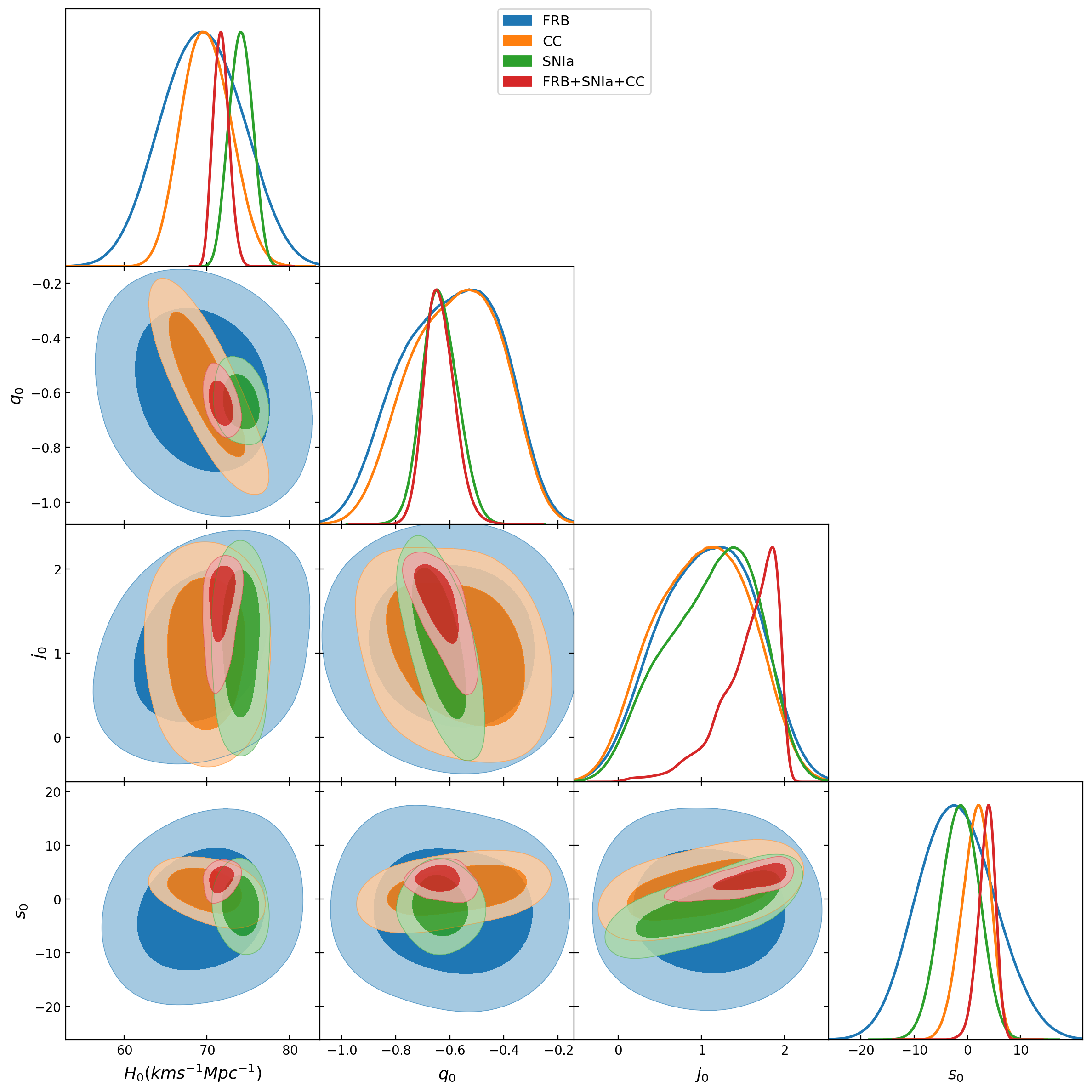
Considering that model II has more theoretical motivations and simulations support it, we have chosen this model for the joint analysis. Nevertheless, it is important to note that even working with model II, the limited number of FRB data and the striking similarity between models I and II results (see Table 2), suggest that there is no huge difference in working with any of them. To perform the joint analysis, we combine the FRB dataset with Cosmic Chronometers and type Ia Supernovae. In this case, the free parameters are , with a Gaussian prior over , with a mean value of , and a standard deviation of given by Camarena & Marra 2021. The total likelihood then is the product:
| (31) |
The statistical results are summarized in Table 4 and displayed in Fig. 3. Our combined constraint for Hubble constant achieves a precision of . It is worth noting a preference for lower values of when utilising Cosmic Chronometers. This preference holds whether employing the cosmography technique or working within the framework of the model (Moresco et al. 2022; Busti et al. 2014) and, as a result, a subtle tension of arises in comparison to the constraints obtained from type Ia Supernovae, causing such a small precision in the joint constraint. The deceleration parameter achieves a precision of while the jerk has a precision of . Furthermore, it is worth mentioning that although the snap parameter does not align within the region of the model, the inclusion of FRBs in conjunction with Cosmic Chronometers and type Ia Supernovae reduces the error associated with this parameter by approximately .
| Parameter | FRB | CC | SNIa | FRB+CC+SNIa |
|---|---|---|---|---|
6 Discussion
Fast Radio Bursts (FRBs) have become an increasingly valuable tool in cosmological research, with the relation being employed in numerous previous studies. In this work, we expand upon this analysis by introducing the cosmographic expansion of the expression. To assess the reliability of our approach, we consider two distinct models. The first model incorporates straightforward assumptions and treats the host and intergalactic medium (IGM) components as Gaussian distributions. The second model is more intricate, assuming a quasi-Gaussian distribution for the IGM component and a lognormal distribution for the host component. Our results indicate that both approaches yield significant improvements over previous studies that solely relied on the relation, achieving an interesting precision of for model I and for model II for the Hubble parameter () despite the limited number of measured FRBs. According to the standard error formula, we estimate that approximately 2400 FRBs with redshift measurements are required to achieve a similar precision level as the SH0ES collaboration. Fortunately, this goal is within reach in the near future, given the growing number of instruments dedicated to the detection of FRBs. Two prominent upcoming radio telescopes deserve mention: the Square Kilometre Array (SKA) and the Baryon Acoustic Oscillations from Integrated Neutral Gas Observations (BINGO) project. The SKA, renowned for its sub-arcsecond accuracy (Zhang et al. 2023), promises to revolutionize FRB (Fast Radio Burst) research by enabling the detection of thousands of FRBs and their redshift counterparts (Macquart et al. 2015). On the other hand, the BINGO project, currently under construction in Brazil (Abdalla et al. 2022; Santos et al. 2023), focuses specifically on detecting the 21-cm line of neutral hydrogen (HI) and is also expected to be a formidable instrument for FRB detection.
By employing the cosmographic expansion, we successfully estimated the kinematic parameters , , and for both models. Notably, our findings exhibited strong agreement between the two models I and II, but it must be recalled that model II has more theoretical foundations and support from cosmological simulations. Utilising only FRBs, we obtained compelling evidence for the acceleration of the expanding Universe. Moreover, the results from both models indicated the presence of a transitional phase during which the dynamics of the universe underwent a change. However, given the limited constraints on the snap parameter, further data are required to discern whether the accelerated expansion is governed by a constant dark energy component or a time-evolving one.
In addition, the present study has investigated how the cosmographic expansion up to the snap parameter can impact on the estimation of the fraction of baryons in the intergalactic medium (IGM). Our analysis revealed that all the models we considered yielded very consistent results that were in agreement with previous studies. Despite the large statistical errors, we were able to address the missing baryon problem by utilising well-localised FRBs. Our calculations yielded an estimated fraction of baryons in the IGM of , which suggests that the majority of baryons are indeed accounted for in the IGM. This finding is significant because it provides further insight into the distribution of matter in the universe in a model-independent way and could have implications for our understanding of cosmic structure formation.
Based on the results of this study, it is clear that cosmography has played a crucial role in advancing our understanding of FRBs and their usefulness as a cosmological tool. By incorporating higher-order kinematic parameters, such as the snap parameter, we were able to improve the precision of our estimates for the Hubble parameter and the fraction of baryons in the IGM. The high level of consistency between our models and previous studies underscores the reliability of cosmography as a technique for understanding the properties of the universe. Additionally, the continued search for new FRBs and the development of more advanced observational techniques could lead to even more precise estimates of cosmological parameters, further refining our understanding of the evolution of the Universe and its fundamental properties.
Acknowledgements
JASF thanks FAPES for financial support. WSHR thanks FAPES (PRONEM No 503/2020) for the financial support under which this work was carried out. The authors thank V. Marra for his insightful comments on this paper.
Data Availability
The data used in this work is publicly available at https://www.wis-tns.org/ and http://frbhosts.org/#explore.
References
- Abdalla et al. (2022) Abdalla E., et al., 2022, Astronomy & Astrophysics, 664, A14
- Aghanim et al. (2020) Aghanim N., et al., 2020, Astronomy & Astrophysics, 641, A6
- Akahori et al. (2016) Akahori T., Ryu D., Gaensler B. M., 2016, ApJ, 824, 105
- Aviles et al. (2012) Aviles A., Gruber C., Luongo O., Quevedo H., 2012, Physical Review D, 86, 123516
- Aviles et al. (2014) Aviles A., Bravetti A., Capozziello S., Luongo O., 2014, Phys. Rev. D, 90, 043531
- Bannister et al. (2019) Bannister K. W., et al., 2019, Science, 365, 565
- Bargiacchi et al. (2021) Bargiacchi G., Risaliti G., Benetti M., Capozziello S., Lusso E., Saccardi A., Signorini M., 2021, A&A, 649, A65
- Bhandari & Flynn (2021) Bhandari S., Flynn C., 2021, Universe, 7, 85
- Bhandari et al. (2020) Bhandari S., et al., 2020, The Astrophysical Journal Letters, 895, L37
- Bhandari et al. (2022) Bhandari S., et al., 2022, The Astronomical Journal, 163, 69
- Bhardwaj et al. (2021a) Bhardwaj M., et al., 2021a, The Astrophysical Journal Letters, 910, L18
- Bhardwaj et al. (2021b) Bhardwaj M., et al., 2021b, The Astrophysical Journal Letters, 919, L24
- Bochenek et al. (2020) Bochenek C. D., Ravi V., Belov K. V., Hallinan G., Kocz J., Kulkarni S. R., McKenna D. L., 2020, Nature, 587, 59
- Busti et al. (2014) Busti V. C., Clarkson C., Seikel M., 2014, Monthly Notices of the Royal Astronomical Society: Letters, 441, L11
- Camarena & Marra (2021) Camarena D., Marra V., 2021, Monthly Notices of the Royal Astronomical Society, 504, 5164
- Capozziello et al. (2018) Capozziello S., D’Agostino R., Luongo O., 2018, MNRAS, 476, 3924
- Cattoën & Visser (2007) Cattoën C., Visser M., 2007, Classical and Quantum Gravity, 24, 5985
- Chatterjee et al. (2017) Chatterjee S., et al., 2017, Nature, 541, 58
- Chittidi et al. (2021) Chittidi J. S., et al., 2021, The Astrophysical Journal, 922, 173
- Cooke et al. (2018) Cooke R. J., Pettini M., Steidel C. C., 2018, The Astrophysical Journal, 855, 102
- Cordes & Lazio (2002) Cordes J. M., Lazio T. J. W., 2002, arXiv preprint astro-ph/0207156
- Day et al. (2020) Day C. K., et al., 2020, Monthly Notices of the Royal Astronomical Society, 497, 3335
- Deng & Zhang (2014) Deng W., Zhang B., 2014, The Astrophysical Journal Letters, 783, L35
- Fong et al. (2021) Fong W.-f., et al., 2021, The Astrophysical Journal Letters, 919, L23
- Fukugita et al. (1998) Fukugita M., Hogan C., Peebles P., 1998, The Astrophysical Journal, 503, 518
- Gao et al. (2014) Gao H., Li Z., Zhang B., 2014, ApJ, 788, 189
- Gómez-Valent & Amendola (2018) Gómez-Valent A., Amendola L., 2018, Journal of Cosmology and Astroparticle Physics, 2018, 051
- Hagstotz et al. (2022) Hagstotz S., Reischke R., Lilow R., 2022, Monthly Notices of the Royal Astronomical Society, 511, 662
- Handley et al. (2015) Handley W., Hobson M., Lasenby A., 2015, Monthly Notices of the Royal Astronomical Society: Letters, 450, L61
- Heinesen (2021) Heinesen A., 2021, Phys. Rev. D, 104, 123527
- Heintz et al. (2020) Heintz K. E., et al., 2020, The Astrophysical Journal, 903, 152
- Hu & Wang (2022) Hu J. P., Wang F. Y., 2022, A&A, 661, A71
- Jalilvand & Mehrabi (2022) Jalilvand F., Mehrabi A., 2022, The European Physical Journal Plus, 137, 1341
- James et al. (2022) James C., et al., 2022, Monthly Notices of the Royal Astronomical Society, 516, 4862
- Jaroszynski (2019) Jaroszynski M., 2019, Monthly Notices of the Royal Astronomical Society, 484, 1637
- Jesus et al. (2018) Jesus J., Gregório T. M., Andrade-Oliveira F., Valentim R., Matos C. A., 2018, Monthly Notices of the Royal Astronomical Society, 477, 2867
- Jimenez & Loeb (2002) Jimenez R., Loeb A., 2002, The Astrophysical Journal, 573, 37
- Kirsten et al. (2021) Kirsten F., et al., 2021, arXiv preprint arXiv:2105.11445
- Law et al. (2020) Law C. J., et al., 2020, The Astrophysical Journal, 899, 161
- Lazkoz et al. (2013) Lazkoz R., Alcaniz J., Escamilla-Rivera C., Salzano V., Sendra I., 2013, Journal of Cosmology and Astroparticle Physics, 2013, 005
- Lemos et al. (2022) Lemos T., Gonçalves R. S., Carvalho J. C., Alcaniz J. S., 2022, arXiv preprint arXiv:2205.07926
- Li et al. (2020) Li Z., Gao H., Wei J.-J., Yang Y.-P., Zhang B., Zhu Z.-H., 2020, Monthly Notices of the Royal Astronomical Society: Letters, 496, L28
- Lin et al. (2023) Lin H.-N., Tang L., Zou R., 2023, MNRAS, 520, 1324
- Lizardo et al. (2021) Lizardo A., Amante M. H., García-Aspeitia M. A., Magaña J., Motta V., 2021, Monthly Notices of the Royal Astronomical Society, 507, 5720
- Lobo et al. (2020) Lobo F. S. N., Mimoso J. P., Visser M., 2020, J. Cosmology Astropart. Phys., 2020, 043
- Lorimer et al. (2007) Lorimer D. R., Bailes M., McLaughlin M. A., Narkevic D. J., Crawford F., 2007, Science, 318, 777
- Macquart et al. (2015) Macquart J.-P., et al., 2015, arXiv preprint arXiv:1501.07535
- Macquart et al. (2020) Macquart J.-P., et al., 2020, Nature, 581, 391
- Marcote et al. (2020) Marcote B., et al., 2020, Nature, 577, 190
- McQuinn (2013) McQuinn M., 2013, The Astrophysical Journal Letters, 780, L33
- McQuinn (2014) McQuinn M., 2014, ApJ, 780, L33
- Moresco et al. (2022) Moresco M., et al., 2022, Living Reviews in Relativity, 25, 6
- Negrelli et al. (2020) Negrelli C., Kraiselburd L., Landau S., Scóccola C. G., 2020, Journal of Cosmology and Astroparticle Physics, 2020, 015
- Nusser (2016) Nusser A., 2016, ApJ, 821, L2
- Ocker et al. (2021) Ocker S. K., Cordes J. M., Chatterjee S., 2021, ApJ, 911, 102
- Padilla et al. (2021) Padilla L. E., Tellez L. O., Escamilla L. A., Vazquez J. A., 2021, Universe, 7, 213
- Petroff et al. (2019) Petroff E., Hessels J., Lorimer D., 2019, The Astronomy and Astrophysics Review, 27, 1
- Pourojaghi et al. (2022) Pourojaghi S., Zabihi N. F., Malekjani M., 2022, Phys. Rev. D, 106, 123523
- Prochaska & Zheng (2019) Prochaska J. X., Zheng Y., 2019, Monthly Notices of the Royal Astronomical Society, 485, 648
- Prochaska et al. (2019a) Prochaska J. X., Simha S., Law C., Tejos N., et al., 2019a, Zenodo
- Prochaska et al. (2019b) Prochaska J. X., et al., 2019b, Science, 366, 231
- Rajwade et al. (2020) Rajwade K., et al., 2020, Monthly Notices of the Royal Astronomical Society, 495, 3551
- Ravi et al. (2019) Ravi V., et al., 2019, Nature, 572, 352
- Riess et al. (2022) Riess A. G., et al., 2022, The Astrophysical Journal Letters, 934, L7
- Rocha & Martins (2023) Rocha B. A. R., Martins C. J. A. P., 2023, MNRAS, 518, 2853
- Santos et al. (2023) Santos M. V. d., et al., 2023, arXiv preprint arXiv:2308.06805
- Scolnic et al. (2018) Scolnic D. M., et al., 2018, The Astrophysical Journal, 859, 101
- Shao & Zhang (2017) Shao L., Zhang B., 2017, Phys. Rev. D, 95, 123010
- Shull et al. (2012) Shull J. M., Smith B. D., Danforth C. W., 2012, The Astrophysical Journal, 759, 23
- Spitler et al. (2016) Spitler L., et al., 2016, Nature, 531, 202
- Tingay & Kaplan (2016) Tingay S. J., Kaplan D. L., 2016, ApJ, 820, L31
- Visser (2005) Visser M., 2005, General Relativity and Gravitation, 37, 1541
- Wei et al. (2015) Wei J.-J., Gao H., Wu X.-F., Mészáros P., 2015, Phys. Rev. Lett., 115, 261101
- Weinberg (1972) Weinberg S., 1972, Gravitation and cosmology: principles and applications of the general theory of relativity
- Wu et al. (2016) Wu X.-F., et al., 2016, ApJ, 822, L15
- Wu et al. (2020) Wu Q., Yu H., Wang F., 2020, The Astrophysical Journal, 895, 33
- Wu et al. (2022) Wu Q., Zhang G.-Q., Wang F.-Y., 2022, Monthly Notices of the Royal Astronomical Society: Letters, 515, L1
- Yang et al. (2022) Yang K., Wu Q., Wang F., 2022, The Astrophysical Journal Letters, 940, L29
- Yao et al. (2017) Yao J., Manchester R., Wang N., 2017, The Astrophysical Journal, 835, 29
- Zhang (2020) Zhang B., 2020, Nature, 587, 45
- Zhang et al. (2023) Zhang J.-G., Zhao Z.-W., Li Y., Zhang J.-F., Li D., Zhang X., 2023, arXiv preprint arXiv:2307.01605
- Zhao et al. (2022) Zhao Z.-W., Zhang J.-G., Li Y., Zou J.-M., Zhang J.-F., Zhang X., 2022, arXiv preprint arXiv:2212.13433
- Zhou et al. (2014) Zhou B., Li X., Wang T., Fan Y.-Z., Wei D.-M., 2014, Phys. Rev. D, 89, 107303
- Zhou et al. (2022) Zhou D., et al., 2022, Research in Astronomy and Astrophysics, 22, 124001