Learning to Identify Graphs from Node Trajectories
in Multi-Robot Networks

In a networked system, the behavior of one node is influenced by the entire network by means of local interactions with neighboring nodes via Eq. (1). Hence, to identify the existence of interactions among two nodes we need to consider, at least initially, the state information from all the nodes. In this section, we describe an optimization method [28] for scalar states ($s=1$) that finds the underlying graph that best describes the state trajectories of the nodes. When state $\mathbf{x}_{i}$ is scalar, the trajectory $\mathbf{X}(t)$ is an $n\times d$ matrix.

First, we define $\mathbf{Y}(t)\in\mathbb{R}^{n\times n}$ as the Euclidean distance matrix among the node states such that $[\mathbf{Y}(t)]_{ij}=||\mathbf{x}_{i}^{d}(t)-\mathbf{x}_{j}^{d}(t))||_{2}^{2}$ $\forall i,j\in\mathcal{V}(t)$. Then,

where $\circ$ denotes element-wise product and $\|\cdot\|_{1}$ is the L1 norm. We omit the time dependence going forward to simplify the notation because all operations refer to the same instant $t$. Based on Eq. (3), finding $\mathbf{W}$ translates into solving a convex inverse problem [25]:

where $\alpha,\beta>0$ are tuning parameters such that $\alpha$ penalizes the possibility of isolated nodes and $\beta$ encourages graph sparsity. To solve (4) efficiently and with global convergence guarantees, Saboksayr and Mateos [28] proposed a dual reformulation of (4). Since the graph is undirected, we define $\mathbf{w}=\mathsf{vech}(\mathbf{W})$ as the half-vectorization of $\mathbf{W}$. Let $\mathbf{y}=\mathsf{vec}(\mathbf{Y})$ be the vectorization of $\mathbf{Y}$ and $\mathbb{I}$ be the indicator function such that $\mathbb{I}\{\mathbf{w}\geq 0\}=0$ and $\infty$ otherwise, where the operation $\geq$ is applied element-wise. Finally, $\mathbf{S}\in\{0,1\}^{n\times\frac{n(n-1)}{2}}$ is the operator that satisfies $\mathbf{W}\mathbf{1}_{n}=\mathbf{S}\mathbf{w}$. This leads to the unconstrained optimization problem

Eq. (5) can be solved by accelerated dual proximal gradient methods with guarantees of global convergence, proved by Beck and Teboulle [29] in the general case, and by Saboksayr and Mateos [28] in the specific case of Eq. (5). In particular, we exploit the analytical expressions derived in [28], summarized in Algorithm 1.

The algorithm iterates until convergence or a certain number of iterations $K\in\mathbb{N}$ is reached. The current iteration is denoted by $k$ and $\bm{\lambda}_{k}$ denotes the Lagrange multipliers of the dual optimization problem of Eq. (5). Algorithm 1 alternates between weighted adjacency matrix and Lagrange multipliers’ updates. Once the algorithm terminates, the graph adjacency matrix is recovered from $\mathbf{w}_{k}$. Interestingly, the stability of the training process is not affected by the $\max$ operator in line 5 of Algorithm 1. At the boundary $\frac{\mathbf{S}^{\top}\bm{\omega}_{k}-2\mathbf{y}}{2\beta}=\mathbf{0}$, the gradient can be smooth by, e.g., using an approximated value like in Pytorch [42].

Besides the global convergence[28], which implies robustness against initializations, Algorithm 1 is efficient to compute so, at each instant, sufficient iterations can be run to ensure convergence to the weighted adjacency matrix that best describes the node state trajectories defined over the Euclidean space.

To use Algorithm 1 for graph identification, the node state trajectories must be encoded to a feature space of dimension $s=1$. On the other hand, the cost function in Eq. (5) is taken with respect to the distance between state trajectories in Euclidean space, so the solution might not reflect the best topology given $\mathbf{X}(t)$ because the interactions may be determined by state proximity in a different space. Therefore, the encoding must be such that the Euclidean distance is the one that best reflects the distances among node trajectories. In addition, the encoding must handle a time-varying number of nodes and adjust to changes in the graph connectivity. To address all these points, in this section we develop a neural network encoder using self-attention [30] to extract suitable features from the node state trajectories.

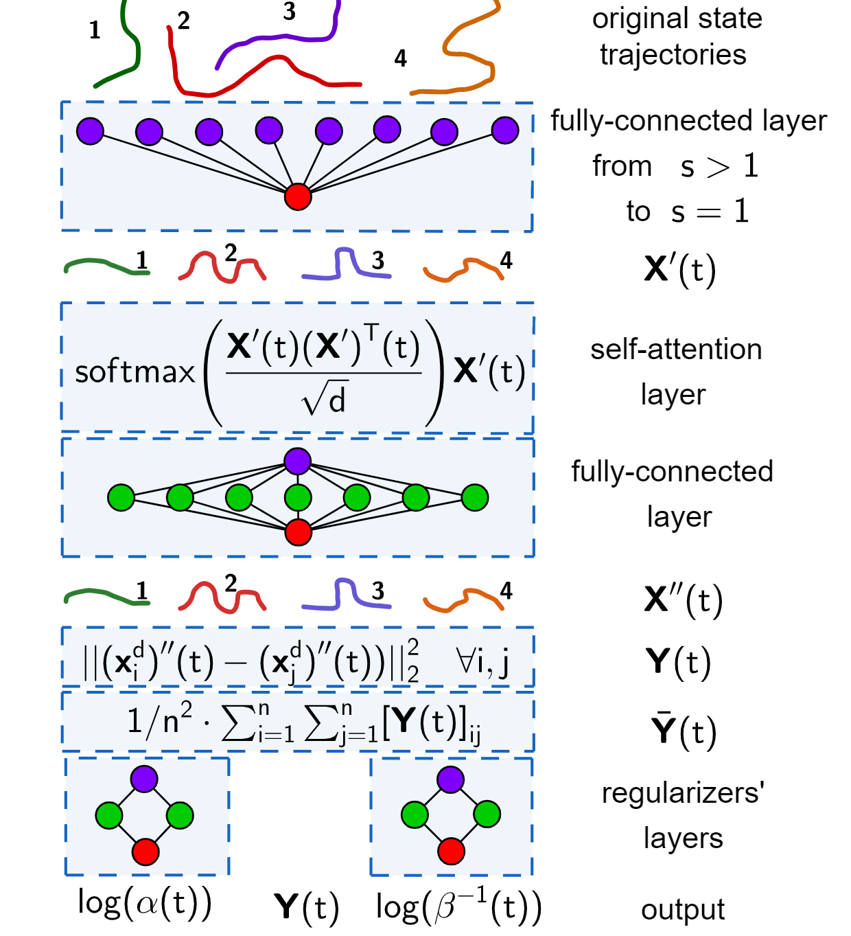
The encoder architecture is illustrated in Fig. 1. First, a fully connected network projects a node state to a feature state of dimension $s=1$. The input is $\mathbf{x}^{d}_{i}(t)$, so the network is applied to every node state and trajectory. The result is a matrix $\mathbf{X}^{\prime}(t)$ that is $n\times d$ as required by the optimization problem in Eq. (5). After that, a self-attention layer processes $\mathbf{X}^{\prime}(t)$ according to the relationships found in the attention map $\mathbf{X}^{\prime}(t)(\mathbf{X}^{\prime})^{T}(t)/\sqrt{d}$, using the operation $\mathsf{softmax}(\mathbf{X}^{\prime}(t)(\mathbf{X}^{\prime})^{T}(t)/\sqrt{d})\mathbf{X}^{\prime}(t)$ with $\mathbf{X}^{\prime}(t)$ the query, key and value matrices. Finally, another fully connected network processes every $(\mathbf{x}_{i}^{d})^{\prime}(t)$ to obtain a new matrix $\mathbf{X}^{\prime\prime}(t)$ that is $n\times d$, composed by the individual trajectories $(\mathbf{x}^{d}_{i})^{\prime\prime}(t)$. These feature trajectories are then used to compute the distance matrix $\mathbf{Y}(t)$. The encoder has an additional module that uses the mean of $\mathbf{Y}(t)$, $\bar{\mathbf{Y}}(t)=\frac{1}{n^{2}}\sum_{i=1}^{n}\sum_{j=1}^{n}[\mathbf{Y}(t)]_{ij}$, to compute the parameters $\alpha(t)$ and $\beta(t)$ of Algorithm 1. The logarithm is considered because sparsity is determined by the difference in the order of magnitude between $\alpha(t)$ and $\beta(t)$.

The encoder network, thanks to the self-attention structure, handles graphs of different configurations in the number of nodes and the intensity of interactions. Furthermore, it not only projects the state trajectories to a convenient feature space, but also provides the parameters for Algorithm 1. Thus, the encoder can be trained to adjust the connectivity depending on the state trajectories. For instance, in a multi-robot flocking task like the one used for evaluation in Section IV, the robots can depart from a spread initial condition and gather in a more compact formation. We remark that the design of the self-attention encoder is not limited to the proposed architecture. Depending on the complexity of the task, the encoder can be increased in depth and number of parameters to ensure that the dimensionality reduction captures all the behaviors of the multi-robot team.

The combination of the fast convex optimization algorithm described in Section III-A and the encoder detailed in Section III-B leads to a learning architecture for graph topology identification from node state trajectories, presented in Fig. 2. The self-attention encoder receives the state trajectories of the multi-robot team. The outputs of the encoder are the one-dimensional feature trajectories of the multi-robot team and the $\alpha$ and $\beta$ regularizers of Algorithm 1. Algorithm 1 is then executed using the feature trajectories as input, providing the discovered topology. To train the model, we use the following loss function:

In the loss function, $\hat{\mathbf{w}}$ refers to the vectorized form of the ground-truth weighted adjacency matrix $\mathbf{W}$. Moreover, $(\bullet)^{*}$ denotes the adjoint of a graph. More precisely, $\mathbf{W}^{*}$ is the weighted adjacency matrix such that $[\mathbf{W}^{*}]_{ij}=0$ if $[\mathbf{W}]_{ij}\neq 0$, $[\mathbf{W}^{*}]_{ij}>0$ if $[\mathbf{W}]_{ij}=0$, and $\mathbf{W}^{*}\mathbf{1}_{n}=\mathbf{W}\mathbf{1}_{n}$. We compute each $[\mathbf{W}^{*}]_{ij}>0$ as $[\mathbf{W}\mathbf{1}_{n}]_{i}/n_{i}^{*}$, where $n_{i}^{*}$ is the number of non-zero elements of the $i-$th row of $\mathbf{W}^{*}$. Thus, $\mathbf{w}^{*}_{k}$ and $\hat{\mathbf{w}}^{*}$ refer to the adjoints of the identified and ground-truth weighted adjacency matrices. The use of the difference of adjoint graphs is to avoid degenerate solutions. For instance, if the ground-truth graph is very sparse, the training might tend to overfit to a graph with no edges unless the adjoint difference is part of the loss. We consider that each iteration of Algorithm 1 is a training step.

Finally, one consideration is in order. Algorithm 1 and optimizations (4)-(5) all provide the optimal graph topology in the state smoothness sense. However, there is one reason for using Algorithm 1 instead of (4) and (5) beyond the fast convergence. The training of the proposed neural network requires to backpropagate the gradients of the loss function with respect to the output through the complete neural network. In our case, the gradients are propagated backward through the steps of Algorithm 1 and the self-attention encoder. Our proposed approach benefits from the fact that these steps are analytical equations rather than an optimization problem as (4) and (5). They are solved by gradient based methods, so, to backpropagate through them, we would need to the gradients of the optimization gradients, which are computationally intractable and numerically unstable. Besides, (4) has constraints and (5) as a non-differentiable indicator function, leading to additional difficulties for the training of the neural network.

Following the setup proposed in many graph identification works [7, 43, 6, 26, 44, 45, 27, 28, 22, 24], we consider a multi-robot formation problem where the position of the robots is given by an Erdős-Rényi random graph [46]. For the training of the neural network, a single graph is instantiated with edge probability $p=0.2$ and a number of robots $n=50$, to study the performance of the proposed approach in a sparse and large multi-robot network. We note that the edge density of the graph $\rho(\mathcal{G})=p$. Different from other works, instead of considering scalars, the robot state is determined by their 2D position, i.e., $s=2$. The states are generated using the following Gaussian random process:

where $\hat{\mathbf{L}}^{\dagger}$ is the pseudoinverse of the ground-truth Laplacian, $\sigma=0.1$ is the noise level that simulates potential uncertainty in the position of the robots, and $\mathbf{x}_{x}(t)$ and $\mathbf{x}_{y}(t)$ refer to the $x$-position and $y$-position of the robots at instant $t$. The covariance is chosen in this way to force that the position of the robots at each instant is correlated to their neighbors, following the state-of-the-art [7, 28] (see [7] for further details). We generate $d=10000$ samples for training. The other training hyperparameters are detailed in Appendix A. To assess the performance of our approach, we randomly generate $18$ test sets composed by $20$ Erdős-Rényi random graphs each, generated from the combination of the following hyperparameters: $n=\{10,20,30,40,50,60\}$ and $p=\{0.1,0.2,0.4\}$. All of them are formed by $d=10000$ samples. We set $K=2000$ to ensure convergence. To assess performance, we use the Mean Absolute Error (MAE) between the ground-truth and the identified weights $\frac{1}{n^{2}}\sum_{i}^{n}\sum_{j}^{n}|[\hat{\mathbf{W}}]_{ij}-[\mathbf{W}]_{ij}|$. We compare our proposal with the state-of-the-art algorithm in [28], which is the closest to our problem assumptions, tuning the parameters according to the procedures detailed in [25, 26, 27]. Since this algorithm only allows scalar trajectories, we apply their algorithm once per state dimension, computing the average graph.

Fig. 3 shows the MAE for the different number of robots and edge probabilities. Our proposed approach surpasses the state-of-the-art in one order of magnitude for all the configurations. It is seen how the learned neural network generalizes to different number of robots, achieving a similar performance in terms of MAE. Therefore, the training has been able to learn a good encoding of the state trajectories and identifies a good $\alpha$ and $\beta$. We emphasize that the training is conducted with just one graph. The learned neural network does not generalize to $\rho(\mathcal{G})=p=0.4$ since only a single graph with $\rho(\mathcal{G})=p=0.2$ has been used for training.

Figs. 4, 5 and 6 show some qualitative results. The weights of the existing edges are accurately identified in graphs with a similar number of robots than in training (Fig. 4), different numbers of robots (Fig. 5) and edge densities (Fig. 6). The intensity of the colors in the discovered graphs is lower than in the ground-truth graphs because there are a few outlier weights with a greater value compared to the ground-truth, so the color scales of $\mathbf{W}$ and $\hat{\mathbf{W}}$ are different. Since the $\hat{\mathbf{W}}$ from the Erdős-Rényi graphs are such that $[\hat{\mathbf{W}}]_{ij}=\{0,1\}$ and to verify that our approach is successful at capturing the existence or absence of edges, the right panels of Figs. 4, 5 and 6 show the difference between identified and ground-truth weighted adjacency matrices, but thresholding to zero all the elements such that $|[\hat{\mathbf{W}}]_{ij}-[\mathbf{W}]_{ij}|<10^{-5}$. Note that this threshold is to remove edges whose order of magnitude is far from the weights of an existing edge. With a correct threshold, the existence or absence of edges is correctly identified for all configurations, except for the case of $\rho(\mathcal{G})=p=0.4$, where the number of edges is underestimated because only a single graph with $\rho(\mathcal{G})=p=0.2$ has been used for the training of the neural network.

The next experiment evaluates our approach when it is trained with a variety of graph edge densities. We study our proposed approach in a multi-robot flocking problem, where the state is defined by the 2D position the robots, so $s=2$. Robot trajectories are generated using the controller proposed in [38], parameterized as detailed in Appendix A. The training set is generated with a sparsity pattern determined by the desired inter robot distance $\rho=0.7$m and communication radius $r_{comm}=1.2$m, simulated through $6$s with a sample time of $0.04$s, and where the robots are uniformly spawned in a square of $5\times 5$m. The trajectories are then split in sub-trajectories of $d=10$, each of them associated to a graph resulting from the average of the $d$ samples. This leads to a training set of graphs with edge densities from $5\%$ to $95\%$. The test cases are generated with the following configurations, one trajectory each: (1) $\rho=0.7$m and $r_{comm}=1.2$m; (2) $\rho=1.0$m and $r_{comm}=1.2$m; and (3) $\rho=0.7$m, $r_{comm}=1.2$m and a compact initialization in a square $2\times 2$m. The desired position of the flock is always $x^{*}=y^{*}=0.0$m. The training of the neural network takes $150000$ steps. Every $500$ steps, one graph with its associated sub-trajectories is uniformly randomly picked, initializing the optimization module each time.

The results in Fig. 7 show how the MAE evolves as a function of the edge density and flocking configuration. For all the cases, our approach outperforms the state-of-the-art by more than one order of magnitude. Compared to the formation problem, the difference now is greater because the dynamics of the robots under the flocking controller are nonlinear. Moreover, in the state-of-the-art algorithms, $\alpha$ and $\beta$ are static, so the output is not able to adjust to changes in edge density. In contrast, our approach adjusts the optimization regularizers and provides the latent feature trajectories that best fit the flocking task, concluding that our approach has learned to adapt the parameters of the optimization method to the observed edge probability/density. Compared to the formation task, the learned neural network achieves a good performance for the different edge densities because the training set is diverse in this aspect. The MAE in Fig. 7 is specially good in very sparse networks ($\rho(\mathcal{G})<0.25$). As observed in Fig. 8, the relative value among the discovered weights is correctly identified, whereas the value of these weights with respect to the ground-truth $\hat{\mathbf{W}}$ vary depending on the edge density of the graph. Looking at Fig. 8, for sparse, medium and dense graphs the identified weights tend to be lower, similar and greater than in the ground-truth graph. This also explains why the MAE in Fig. 7 grows with the edge density. Besides, the neural network predicts a greater number of cliques, as in the middle row of Fig. 8. These behaviors require further investigation. As future work, We also plan to conduct ablation studies to analyze the impact of the dataset edge density variety in the generalization capabilities of our approach.

References

- [1] R. P. Monti, P. Hellyer, D. Sharp, R. Leech, C. Anagnostopoulos, and G. Montana, “Estimating time-varying brain connectivity networks from functional MRI time series,” NeuroImage, vol. 103, pp. 427–443, 2014.
- [2] W. Huang, T. A. Bolton, J. D. Medaglia, D. S. Bassett, A. Ribeiro, and D. Van De Ville, “A graph signal processing perspective on functional brain imaging,” Proceedings of the IEEE, vol. 106, no. 5, pp. 868–885, 2018.
- [3] E. Nozari, R. Planas, and J. Cortés, “Structural characterization of oscillations in brain networks with rate dynamics,” Automatica, vol. 146, p. 110653, 2022.
- [4] A. Julius, M. Zavlanos, S. Boyd, and G. J. Pappas, “Genetic network identification using convex programming,” IET Systems Biology, vol. 3, no. 3, pp. 155–166, 2009.
- [5] M. Nabi-Abdolyousefi and M. Mesbahi, “Network identification via node knockout,” IEEE Transactions on Automatic Control, vol. 57, no. 12, pp. 3214–3219, 2012.
- [6] G. B. Giannakis, Y. Shen, and G. V. Karanikolas, “Topology identification and learning over graphs: Accounting for nonlinearities and dynamics,” Proceedings of the IEEE, vol. 106, no. 5, pp. 787–807, 2018.
- [7] X. Dong, D. Thanou, P. Frossard, and P. Vandergheynst, “Learning Laplacian matrix in smooth graph signal representations,” IEEE Transactions on Signal Processing, vol. 64, no. 23, pp. 6160–6173, 2016.
- [8] R. Shafipour, S. Segarra, A. G. Marques, and G. Mateos, “Network topology inference from non-stationary graph signals,” in IEEE International Conference on Acoustics, Speech and Signal Processing, 2017, pp. 5870–5874.
- [9] E. Montijano, G. Oliva, and A. Gasparri, “Distributed estimation and control of node centrality in undirected asymmetric networks,” IEEE Trans. on Automatic Control, vol. 66, no. 5, pp. 2304–2311, 2020.
- [10] B. Pasdeloup, V. Gripon, G. Mercier, D. Pastor, and M. G. Rabbat, “Characterization and inference of graph diffusion processes from observations of stationary signals,” IEEE Transactions on Signal and Information Processing over Networks, vol. 4, no. 3, pp. 481–496, 2017.
- [11] D. Thanou, X. Dong, D. Kressner, and P. Frossard, “Learning heat diffusion graphs,” IEEE Transactions on Signal and Information Processing over Networks, vol. 3, no. 3, pp. 484–499, 2017.
- [12] M. Timme, “Revealing network connectivity from response dynamics,” Physical Review Letters, vol. 98, no. 22, p. 224101, 2007.
- [13] D. Napoletani and T. D. Sauer, “Reconstructing the topology of sparsely connected dynamical networks,” Physical Review E, vol. 77, no. 2, p. 026103, 2008.
- [14] X. Dong, D. Thanou, M. Rabbat, and P. Frossard, “Learning graphs from data: A signal representation perspective,” IEEE Signal Processing Magazine, vol. 36, no. 3, pp. 44–63, 2019.
- [15] G. Mateos, S. Segarra, A. G. Marques, and A. Ribeiro, “Connecting the dots: Identifying network structure via graph signal processing,” IEEE Signal Processing Magazine, vol. 36, no. 3, pp. 16–43, 2019.
- [16] F. Xia, K. Sun, S. Yu, A. Aziz, L. Wan, S. Pan, and H. Liu, “Graph learning: A survey,” IEEE Transactions on Artificial Intelligence, vol. 2, no. 2, pp. 109–127, 2021.
- [17] F. Rossi, S. Bandyopadhyay, M. T. Wolf, and M. Pavone, “Multi-agent algorithms for collective behavior: A structural and application-focused atlas,” arXiv preprint arXiv:2103.11067, 2021.
- [18] G. Shi, W. Hönig, Y. Yue, and S.-J. Chung, “Neural-swarm: Decentralized close-proximity multirotor control using learned interactions,” in IEEE International Conference on Robotics and Automation. IEEE, 2020, pp. 3241–3247.
- [19] T. Z. Jiahao, L. Pan, and M. A. Hsieh, “Learning to swarm with knowledge-based neural ordinary differential equations,” in International Conference on Robotics and Automation. IEEE, 2022, pp. 6912–6918.
- [20] E. Sebastián, T. Duong, N. Atanasov, E. Montijano, and C. Sagüés, “LEMURS: Learning distributed multi-robot interactions,” in IEEE Int. Conf. on Robotics and Automation, 2023, pp. 7713–7719.
- [21] A. Ortega, P. Frossard, J. Kovačević, J. M. Moura, and P. Vandergheynst, “Graph signal processing: Overview, challenges, and applications,” Proceedings of the IEEE, vol. 106, no. 5, pp. 808–828, 2018.
- [22] S. Segarra, A. G. Marques, G. Mateos, and A. Ribeiro, “Network topology inference from spectral templates,” IEEE Transactions on Signal and Information Processing over Networks, vol. 3, no. 3, pp. 467–483, 2017.
- [23] S. Shahrampour and V. M. Preciado, “Topology identification of directed dynamical networks via power spectral analysis,” IEEE Transactions on Automatic Control, vol. 60, no. 8, pp. 2260–2265, 2014.
- [24] S. Segarra, G. Mateos, A. G. Marques, and A. Ribeiro, “Blind identification of graph filters,” IEEE Transactions on Signal Processing, vol. 65, no. 5, pp. 1146–1159, 2016.
- [25] V. Kalofolias, “How to learn a graph from smooth signals,” in Artificial Intelligence and Statistics, 2016, pp. 920–929.
- [26] V. Kalofolias, A. Loukas, D. Thanou, and P. Frossard, “Learning time varying graphs,” in IEEE International Conference on Acoustics, Speech and Signal Processing, 2017, pp. 2826–2830.
- [27] S. S. Saboksayr, G. Mateos, and M. Cetin, “Online graph learning under smoothness priors,” in IEEE European Signal Processing Conference, 2021, pp. 1820–1824.
- [28] S. S. Saboksayr and G. Mateos, “Accelerated graph learning from smooth signals,” IEEE Signal Processing Letters, vol. 28, pp. 2192–2196, 2021.
- [29] A. Beck and M. Teboulle, “A fast dual proximal gradient algorithm for convex minimization and applications,” Operations Research Letters, vol. 42, no. 1, pp. 1–6, 2014.
- [30] A. Vaswani, N. Shazeer, N. Parmar, J. Uszkoreit, L. Jones, A. N. Gomez, Ł. Kaiser, and I. Polosukhin, “Attention is all you need,” Advances in Neural Information Processing Systems, vol. 30, 2017.
- [31] P. Shaw, J. Uszkoreit, and A. Vaswani, “Self-attention with relative position representations,” arXiv preprint arXiv:1803.02155, 2018.
- [32] N. Kamra, H. Zhu, D. K. Trivedi, M. Zhang, and Y. Liu, “Multi-agent trajectory prediction with fuzzy query attention,” Advances in Neural Information Processing Systems, vol. 33, pp. 22 530–22 541, 2020.
- [33] Q. Li, W. Lin, Z. Liu, and A. Prorok, “Message-aware graph attention networks for large-scale multi-robot path planning,” IEEE Robotics and Automation Letters, vol. 6, no. 3, pp. 5533–5540, 2021.
- [34] Z. Wang and M. Gombolay, “Learning scheduling policies for multi-robot coordination with graph attention networks,” IEEE Robotics and Automation Letters, vol. 5, no. 3, pp. 4509–4516, 2020.
- [35] W. L. Hamilton, “Graph representation learning,” Synthesis Lectures on Artifical Intelligence and Machine Learning, vol. 14, no. 3, pp. 1–159, 2020.
- [36] Y. Wang, Y. Sun, Z. Liu, S. E. Sarma, M. M. Bronstein, and J. M. Solomon, “Dynamic graph CNN for learning on point clouds,” ACM Transactions on Graphics, vol. 38(5), pp. 1–12, 2019.
- [37] P. Goyal, S. R. Chhetri, and A. Canedo, “dyngraph2vec: Capturing network dynamics using dynamic graph representation learning,” Knowledge-Based Systems, vol. 187, p. 104816, 2020.
- [38] R. Olfati-Saber, “Flocking for multi-agent dynamic systems: Algorithms and theory,” IEEE Transactions on Automatic Control, vol. 51, no. 3, pp. 401–420, 2006.
- [39] N. Atanasov, J. Le Ny, K. Daniilidis, and G. J. Pappas, “Decentralized active information acquisition: Theory and application to multi-robot SLAM,” in IEEE International Conference on Robotics and Automation. IEEE, 2015, pp. 4775–4782.
- [40] D. Acemoglu and A. Ozdaglar, “Opinion dynamics and learning in social networks,” Dynamic Games and Applications, vol. 1, pp. 3–49, 2011.
- [41] S. S. Kia, B. Van Scoy, J. Cortes, R. A. Freeman, K. M. Lynch, and S. Martinez, “Tutorial on dynamic average consensus: The problem, its applications, and the algorithms,” IEEE Control Systems Magazine, vol. 39, no. 3, pp. 40–72, 2019.
- [42] A. Paszke, S. Gross, F. Massa, A. Lerer, J. Bradbury, G. Chanan, T. Killeen, Z. Lin, N. Gimelshein, L. Antiga, et al., “Pytorch: An imperative style, high-performance deep learning library,” Advances in neural information processing systems, vol. 32, 2019.
- [43] H. E. Egilmez, E. Pavez, and A. Ortega, “Graph learning from data under Laplacian and structural constraints,” IEEE Journal of Selected Topics in Signal Processing, vol. 11, no. 6, pp. 825–841, 2017.
- [44] J. Mei and J. M. Moura, “Signal processing on graphs: Causal modeling of unstructured data,” IEEE Transactions on Signal Processing, vol. 65, no. 8, pp. 2077–2092, 2016.
- [45] E. Pavez, H. E. Egilmez, and A. Ortega, “Learning graphs with monotone topology properties and multiple connected components,” IEEE Transactions on Signal Processing, vol. 66, no. 9, pp. 2399–2413, 2018.
- [46] P. Erdos and A. Rényi, “On the evolution of random graphs,” Publications of the Mathematical Institute of the Hungarian Academy of Sciences, vol. 5, no. 1, pp. 17–60, 1960.
- [47] D. P. Kingma and J. Ba, “Adam: A method for stochastic optimization,” International Conference on Learning Representations, 2015.