On Invariance, Equivariance, Correlation and Convolution of Spherical Harmonic Representations
for Scalar and Vectorial Data.

Janis Keuper
keuper@imla.ai Affiliation: Institute for Machine Learning and Analytics (IMLA), Offenburg University Affiliation: CC-HPC, Fraunhofer ITWM, Kaiserslautern

Abstract

The mathematical representations of data in the Spherical Harmonic ( ${\cal SH}$ ) domain has recently regained increasing interest in the machine learning community. This technical report gives an in-depth introduction to the theoretical foundation and practical implementation of ${\cal SH}$ representations, summarizing works on rotation invariant and equivariant features, as well as convolutions and exact correlations of signals on spheres. In extension, these methods are then generalized from scalar ${\cal SH}$ representations to Vectorial Harmonics ( ${\cal VH}$ ), providing the same capabilities for 3d vector fields on spheres.

NOTE 1:

This document is a re-publication of a subset of works originally published in my PhD thesis (I changed my last name from Fehr to Keuper):

Fehr, Janis. Local invariant features for 3D image analysis.
PhD Thesis. University of Freiburg, 2009.

Hence, it does NOT provide any references or findings since 2009. The sole intention of this re-publication is to provide old (but still very useful) insights to an Arxiv audience (which occasionally appears not to be aware of pre-Arxiv works).

Please cite the thesis or the original publications:

Fehr, Janis. "Local rotation invariant patch descriptors for 3D vector
fields." 20th International Conference on Pattern Recognition. IEEE, 2010.

Fehr, Janis, Marco Reisert, and Hans Burkhardt. "Fast and accurate rotation
estimation on the 2-sphere without correspondences." 10th European
Conference on Computer Vision, Marseille, France, October 12-18, 2008

Fehr, Janis, and Hans Burkhardt. "Harmonic Shape Histograms for 3D Shape
Classification and Retrieval." MVA. 2007.

Ronneberger, Olaf, Janis Fehr, and Hans Burkhardt. "Voxel-wise gray scale
invariants for simultaneous segmentation and classification." Joint Pattern
Recognition Symposium. Berlin, Heidelberg: Springer Berlin Heidelberg, 2005.

when using this content for your work.

NOTE 2:

The original thesis and publications where all targeting multi-channel volumetric input data given by the target applications at that time. However, the actual methods in the harmonic domain directly extend to other data and applications in most cases.

Introduction and Perquisites

Structure of of the report:

The following report is structured as follows: in this introductory chapter we review the aspects of feature design in general (section 0.2), and take a closer look at local (section 0.3) and invariant features (section 0.2.2).
In chapter 1 we introduce the essential mathematical basics and derive further mathematical techniques needed for the formulation of our features, including correlation and convolution.
Chapter 2 discusses basic implementation issues like sampling problems or parallelization and fills the gap between the continuous mathematical theory and discrete implementation: for each of the following features, we first derive the theoretic foundation in a continuous setting, and then give details on the actual discrete implementation based on these methods.
Then we introduce several different classes of features and their feature extraction algorithms: chapter 3 introduces the class of ${\cal SH}$ -Features, chapter 4 derives new features based on Haar-Integration and finally the chapters 5 and 6 show how we can compute different features on 3D vector fields. An overview of all features which are covered in this work can be found in table 1.
Finally, we evaluate and compare the introduced features on an artificial benchmark (chapter 7).

Feature		Invariance	Input domain	Output domain
${\cal SH}_{abs}$	3.1	r invariance & g robustness	scalar	band-wise scalar
${\cal SH}_{phase}$	3.2	r invariance & g invariance	scalar	band-wise scalar
${\cal SH}_{corr}$	3.3	r invariance & g invariance	scalar	scalar
${\cal SH}_{bispectrum}$	3.4	r invariance & g robustness	scalar	sub-band-wise scalar
2p-Haar	4.1	r invariance & g robustness	scalar	scalar
3p-Haar	4.2	r invariance & g robustness	scalar	scalar
np-Haar	4.3	r invariance & g invariance	scalar	scalar
${\cal VH}_{abs}$	5.1	r invariance & g invariance	vectorial	band-wise scalar
${\cal VH}_{autocorr}$	5.2	r invariance & g invariance	vectorial	scalar
1v-Haar	6.1	r invariance & g invariance	vectorial	scalar
2v-Haar	6.2	r invariance & g invariance	vectorial	scalar
nv-Haar	6.3	r invariance & g invariance	vectorial	scalar

Table 1: Schematic overview of all features with their invariance properties and input/output domains (r = rotation, g = gray-scale).

0.1 Mathematical Notation

$x\in\mathbb{R},x\in\mathbb{C}$	real or complex scalar value
$\Re(x)$	real part of a complex value
$\Im(x)$	imaginary part of a complex value
$\bar{x}$	complex conjugate
${\bf x}\in\mathbb{R}^{n},{\bf x}\in\mathbb{C}^{n}$	n-dimensional position or vector
$X:\mathbb{R}^{n}\rightarrow\mathbb{R},X:\mathbb{Z}^{n}\rightarrow\mathbb{R}$	image function representing a $n$ D scalar image
$X[c_{i}]:\mathbb{R}^{n}\rightarrow\mathbb{R}$	$i$ -th channel of a $m$ -channel $n$ D continuous scalar image
${\bf X}:\mathbb{R}^{n}\rightarrow\mathbb{R}^{m}$	image function representing a $n$ D field of $m$ D vectors
$X({\bf x})\in\mathbb{R}$	scalar value at position ${\bf x}$
${\bf X}({\bf x})\in\mathbb{R}^{n}$	vectorial value at position $\bf{x}$
$\kappa(x)$	non-linear kernel function $\kappa:\mathbb{R}\rightarrow\mathbb{R}$
$T[X]$ and $T[\bf{X}]$	voxel-wise feature extraction
${\cal S}[r]({\bf x}):=\{{\bf x_{i}}\in\mathbb{R}^{n}\|\\|{\bf x}-{\bf x_{i}}\\|=r\}$	spherical neighborhood around ${\bf x}$
${\cal F}(\cdot)$	Fourier transform
${\cal SH}\big(X\|_{{\cal S}[r]({\bf x})}\big)$	Spherical Harmonic transform of a local neighborhood
${\cal SH}[r](X)$	element-wise Spherical Harmonic transform with radius $r$
${\cal VH}\big({\bf X}\|_{{\cal S}[r]({\bf x})}\big)$	Vectorial Harmonic transform of a local neighborhood
${\cal VH}[r]({\bf X})$	element-wise Vectorial Harmonic with radius $r$
$\widehat{X}:={\cal F}(X)$ or $\widehat{X}:={\cal SH}[r](X)$	$X$ transformed into frequency domain
$A\cdot$ B	scalar or voxel-wise multiplication
$\cal{R}_{(\phi,\theta,\psi)}$ or just $\cal{R}$	rotation matrix
$A*B$	convolution in $\mathbb{R}^{n}$ or $S^{2}$
$A\#B$	correlation in $\mathbb{R}^{n}$ or $S^{2}$
$\cal{C}^{*}$	convolution matrix
$\cal{C}^{\#}$	correlation matrix
$\cal{G}$	mathematical group
${g}\in\cal{G}$	group element
${\cal SO}(3)$	rotation group in $\mathbb{R}^{3}$
$\phi,\theta,\psi$	parameterization angles of ${\cal SO}(3)$
$S^{2}$	sphere
$\Phi,\Theta$	parameterization angles of $S^{2}$
$\bf{\nabla}\bf{X}$	vector field containing gradients of scalar field $\bf{X}$
$\bf{\nabla}X(\bf{x})$	gradient at position $\bf{x}$

Table 2: Overview of the mathematical notation used throughout this work.

0.2 General Feature Design

Most pattern recognition tasks can be derived from a very general and basic problem setting: given an arbitrary set of patterns $\{X_{i}|X_{i}\in{\cal X}\}$ , we are looking for some function $\Gamma:X_{i}\rightarrow y_{i}$ which denotes each pattern with a semantic label $y_{i}\in Y$ from the category space $Y\subset\mathbb{Z}$ .
In general, ${\cal X}$ contains all possible patterns, which are usually defined as the digitalized signals obtained from a sensor capturing the “real world” (see figure 1). $Y$ holds the semantic meaning (categorization) of the real world, where each category $y_{i}$ defines an equivalence class.
The actual task of assigning the label $y_{i}$ is called classification and $\Gamma$ is often referred as decision function or classifier which should hold:

X_{1}\sim_{y}X_{2}\Leftrightarrow\Gamma(X_{1})=\Gamma(X_{2}).

(1)

Refer to caption — Figure 1: Idealized pattern recognition pipeline on images: in general, we try to reduce the problem complexity from continuous real world data to an 1D categorization space. The semantic match of real world objects to such categories is given by definitions based the human perception and thinking.

The most crucial step towards a suitable $\Gamma$ is to find an adequate equality measure on $X$ . Since the notion of equivalence of real world objects is given by the human perception and is often highly semantic, it is usually very hard to construct a measure which fulfills (1).

In practice, there are two strategies to tackle this problem: learning and feature extraction - which are usually combined.
The first approach tries to learn $\Gamma$ from a set of training examples - we discuss this method in depth in part II of this work. However, most practical problems are too complex to construct or learn $\Gamma$ directly by raw “pattern matching”. Such a “pattern matching” is usually too expensive in terms of computational complexity, or even completely intractable in cases with a large intra class variance, e.g. if patterns of the same equivalence class are allowed to have strong variations in their appearance.
The second approach tries to solve the problem by simplifying the original problem: the goal is to find a reduced representation $\widetilde{X}$ of the original pattern $X$ which still preserves the distinctive properties of $X$ . A commonly used analogy for the feature concept is the notion of “fingerprints” which are extracted from patterns to help to find a simpler classifier $\Gamma^{\prime}$ which holds:

X_{1}\sim_{y}X_{2}\Leftrightarrow\Gamma(X_{1})=\Gamma(X_{2})\Leftrightarrow\Gamma^{\prime}(\widetilde{X_{1}})=\Gamma^{\prime}(\widetilde{X_{2}}).

(2)

Either a perfect feature extraction or a perfect classifier would solve the problem completely, but in practice we have to combine both methods to obtain reasonable results: We use features to reduce the problem and then learn $\Gamma^{\prime}$ (see figure 2).

0.2.1 Feature Extraction

We formalize the feature extraction in form of some function $T(X_{i})$ which maps all input signals ${X_{i}}$ into the so-called feature space $\widetilde{\cal X}$ :

\widetilde{X_{i}}=:T(X_{i}).

(3)

For the theoretical case of a “perfect” feature, $T(X_{i})$ maps all input signals ${X_{i}}$ belonging to the same semantic class with label $y_{i}$ onto one point $\widetilde{X_{i}}$ in this features space:

X_{1}\sim_{y}X_{2}\Leftrightarrow T(X_{1})=T(X_{2}).

(4)

As mentioned before, the nature of practical problems includes that there are intra class variations which make things more complicated. We model these intra class variations by transformations $h_{i}\in H_{y}$ , where $H_{y}$ is the set of all possible transformations, which do not change the label $y$ of the ideal class template $X_{y}$ :

X_{i}:=h_{i}X_{y}.

(5)

If it is impossible to construct the “perfect” feature for a practical application, the goal is to find feature mappings $T(h{X_{y}})$ which at least fulfill the following properties:

•

(I) size: the feature space should be much smaller than the pattern space: $n<<<p$ with $\widetilde{\cal X}\subset\mathbb{R}^{n},{\cal X}\subset\mathbb{R}^{p}$ .
•

(II) continuity: small changes in the input pattern $X_{i}$ should have only small effects in feature space $\widetilde{\cal X}$
•

(III) cluster preservation: local neighborhoods should be transfered from input to feature space

If the extracted feature $\widetilde{X_{i}}$ adheres to these properties, $\widetilde{\cal X}$ provides several advantages for the further construction or learning of $\Gamma$ : first, (I) drastically reduces the computational complexity and second, (II) and (III) make it possible to introduce a meaningful similarity measure on $\widetilde{\cal X}$ (like a simple Euclidean-Norm), which is an essential precondition to the application of learning algorithms (see part II).

Still, the question remains how to construct features which hold the properties I-III. While size property (I) is rather easy to meet, continuity (II) and cluster preservation (III) are more difficult to obtain. This leads us to the notions of invariance and robustness of features, which are central to the methods presented in this work.

0.2.2 Invariance

Feature extraction methods are strongly interlaced with the concept of invariance. The basic idea of invariant features is to construct $T(X)$ in such a way that the effect of those transformations $h_{i}\in H_{y}$ (5) which are not affecting the semantic class label $y$ of $X$ , e.g. $X\sim_{y}h_{i}X$ , is canceled out by $T$ :

T(h_{i}{X_{y}})=\widetilde{X_{y}},\forall h_{i}\in H_{y}.

(6)

For two signals ${X_{1}}$ and ${X_{2}}$ which are considered to be equivalent under a certain transformation $h_{i}\in H_{y}$ , ${X_{1}}\overset{h_{i}}{\sim}{X_{2}}$ , the necessary condition [4] for invariance against $h_{i}$ is:

{X_{1}}\overset{h_{i}}{\sim}{X_{2}}\Rightarrow T({X_{1}})=\widetilde{X_{1}}=\widetilde{X_{2}}=T({X_{2}}).

(7)

In order to achieve completeness [4], $T$ has to hold:

T({X_{1}})=T({X_{2}})\Rightarrow{X_{1}}\overset{h_{i}}{\sim}{X_{2}}.

(8)

In most cases the mathematical completeness condition is too strict, since it is not practicable to have a distinct mapping for every theoretically possible pattern ${X_{i}}$ . However, with only little a priori knowledge, one can determine a sufficient subset of likely patterns ${\cal X}^{\prime}$ . If (8) holds for all ${X_{i}},{X_{j}}\in{\cal X}^{\prime}$ , separability [4] can be guaranteed for the likely patterns.
It is straightforward to see that a feature which holds the necessary condition (7) and achieves at least separability meets the properties II and III.

Group Transformations

The construction of an invariant feature requires that we are able to model the allowed transformations $h_{i}\in H_{y}$ of the equivalence class with label $y$ . In general this is a hard and sometimes infeasible task, e.g. just think of arbitrary deformations. However, for the subset of transformations $G_{y}\subset H_{y}$ , where $G_{y}$ forms a compact mathematical group, we have sophisticated mathematical tools to model the individual transformations $g_{i}\in G_{y}$ .
Luckily, many practically relevant transformations like rotations are groups or can easily be transformed to groups, e.g. translations if we consider cyclic translations. Overall, we can formulate translations, rotations, shrinking, shearing and even affine mappings as group operations [5].

General Techniques For The Construction Of Invariant Features

In general, there are three generic ways of constructing invariant features: by normalization, derivation and integration [5]. For allowed transformations $H_{y}$ , the individual transformations $h\in H_{y}$ differ only by their associated set of parameters $\boldsymbol{\mathbf{\lambda}}$ , which cover the degrees of freedom under $H_{y}$ . The most popular method for invariant feature construction is to eliminate the influence of $\boldsymbol{\mathbf{\lambda}}$ via normalization of the class members $X_{i}:=h_{\lambda}X_{y}$ with a class template $X_{y}$ .
We apply normalization techniques in the following features: ${\cal SH}_{abs}$ (chapter 3.1), ${\cal SH}_{phase}$ (chapter 3.2), ${\cal SH}_{bispectrum}$ , and ${\cal VH}_{abs}$ (chapter 5.1)
However, it should be noted that normalization techniques in general tend to suffer in cases of noisy or partially corrupted data and are often totally infeasible for complex data where no normalized template can be found.

A second possibility is the elimination of $\boldsymbol{\mathbf{\lambda}}$ via derivation:

{\partial T(g_{\boldsymbol{\mathbf{\lambda}}}{X_{i}})\over\partial\lambda}\equiv 0.

(9)

The resulting differential equations can be solved using Lie-Theory [23] approaches, but in practice it is often very difficult to obtain solutions to the differential equations.

Finally, the approach which has been proposed by [45] can be applied on the subset of group transformations: It generates invariant features via Haar-Integration over all degrees of freedom of the transformation group $G$ . We take an in-depth look at the Haar-Integration approach in chapter 4 and apply it in several of our features: 2p-Haar (chapter 4.1), 3p-Haar (chapter 4.2), np-Haar (chapter 4.3), 1v-Haar (chapter 6.1), 2v-Haar (chapter 6.2) and nv-Haar (chapter 6.3).

For many practical applications invariance can be achieved by the combination of several different approaches: we can split transformations $h$ into a combination of several independent transformations $h:=h_{1}\circ h_{2}\circ\dots$ , where $h_{1}$ might be a group transformation like i.e. rotation and $h_{2}$ a non-group transformation like gray-scale changes.

The concept of invariance provides us with a powerful tool for the construction of features which is suitable for a wide range of problems. However, there are still many practically relevant cases where some of the underlying transformations $h_{i}$ cannot be sufficiently modelled, or are even partially unknown. Then it becomes very hard or impossible to construct invariant features. In these cases we have to fall back to the sub-optimal strategy to construct robust instead of invariant features.

0.2.3 Robustness

Robustness is a weaker version of invariance: if we are not able to cancel out the effect of the transformations $h_{i}$ like in (7), we can at least try to minimize the impact of these intra class variations.
Given ${X_{1}}\overset{h}{\sim}{X_{2}},{X_{1}},{X_{2}}\in{\cal X}$ , we are looking for a feature $T$ which maps ${X_{1}},{X_{2}}$ in such a way that the intra class variance in $\widetilde{\cal X}$ is smaller than the extra class distances given some distance measure $d$ in $\widetilde{\cal X}$ :

{X_{1}}\overset{h_{i}}{\sim}{X_{2}}\Rightarrow d\big(T({X_{1}}),T({X_{2}})\big)<d\big(T({X_{1,2}}),T({X^{\prime}})\big),\text{\quad}\forall X^{\prime}\in{\cal X}:X^{\prime}\neg\overset{h_{i}}{\sim}X_{1,2}.

(10)

It is obvious that the robustness property (10) directly realizes the feature properties II and III. In practice, robustness is often achieved by simplified approximations of complex intraclass variations, e.g. linear approximations of actually non-linear transformations $h_{i}$ . In theses cases, we often use an even weaker definition of robustness and demand that (10) has only to hold for most but not all $X^{\prime}\in{\cal X}$ .

0.2.4 Equivariance

For some applications it is desirable to explicitly transfer the variations to the feature space:

{X_{1}}\overset{h_{i}}{\sim}{X_{2}}\Rightarrow T({X_{1}})=h_{i}T({X_{2}}).

(11)

These features are called equivariant, and are often used to compute the parameters of known transformations $h_{i}$ .

0.3 Local Features

The feature definition in the last section (0.2.1) considered only the extraction of so-called “global” features, i.e. features are extracted as descriptors $\widetilde{X_{i}}=T(X_{i})$ (or “Fingerprints”) of the entire pattern $X_{i}$ . This global approach is suitable for many pattern recognition problems, especially when the patterns are taken from prior segmented objects (see part III). In other cases, it can be favorable to describe a global pattern as an ensemble of locally constrained sub-patterns. Such a local approach is suitable for object retrieval, object detection in unsegmented data, or data segmentation itself (see part III).

0.3.1 Local Features on 3D Volume Data

Throughout the rest of this work we deal with 3D volume data or 3D vector fields. In general we derive the theoretical background of the local features in settings of continuous 3D volumes, which we define as functions $X:\mathbb{R}^{3}\rightarrow\mathbb{R}^{m}$ with values $X({\bf x})\in\mathbb{R}^{m}$ at evaluation coordinates ${\bf x}\in\mathbb{R}^{3}$ . We then transfer the feature algorithms to operate on the practical relevant discrete 3D volume grids: $X:\mathbb{Z}^{3}\rightarrow\mathbb{R}^{m}$ , where we often refer to the position ${\bf x}$ as a “voxel”.

Given 3D volume data, we capture the locality of the features extracted from $X$ in terms of a spatial constraining of the underlying sub-pattern. More precisely, we define a sub-pattern as “local neighborhood” around a data point at ${\bf x}$ with the associated local feature $\widetilde{X({\bf x})}$ .
Further, we parameterize the local “neighborhood” in concentric spheres with radii $r$ around ${\bf x}$ . This has several advantages over a rectangular definition of the “local neighborhood”:
First, we can easily define the elements of the sub-pattern by a single parameter $r$ using the following notation for the sub-pattern around ${\bf x}$ :

{\cal S}[r]\left({\bf x}\right):=\{{\bf x}_{i}\in\mathbb{R}^{3}|\|{\bf x}-{\bf x}_{i}\|_{2}=r\}.

(12)

Second, we can address all points in ${\cal S}[r]\left({\bf x}\right)$ via the parameterization in radius $r$ and the spherical coordinates $(\Phi,\Theta$ ) - see section 1.2 for more details on the parameterization. And finally, we can rely on a well known and sound mathematical theory to handle signals (patterns) in spherical coordinates which provides us with very useful tools to handle common transformations such as rotations.
We give an in-depth introduction and further extensions to this mathematical basis for our local features in chapter 1.

Gray-Scale Data

In cases where the 3D volume data is scalar $X:\mathbb{R}^{3}\rightarrow\mathbb{R}$ , we can directly apply the locality definition (12). Note, that we usually refer to scalar data as “gray-scale” data, this term is derived from the usual data visualization as gray-scale images - even though the scalar values might encode arbitrary information. Analogous to this, we denote intensity changes as gray-scale changes.
For many pattern recognition tasks on scalar 3D volume data we like to obtain gray-scale and rotation invariant local features in order to cancel out the dominant transformations which act locally. Other transformations of the data do not act locally, like translations, or are very hard to model like arbitrary deformations. In these cases we try to obtain local robustness, which is usually easier to obtain than global robustness since the local affect of complex global transformations is limited in most cases.

Multi-Channel Data

In many cases we face volumes with data which holds more than a single scalar value at each position ${\bf x}$ . Then we define $X:\mathbb{R}^{3}\rightarrow\mathbb{R}^{m}$ for data with $m$ scalar values per position. The classic example could be a RGB color coding at each voxel, but we might also have other multi-modal data with an arbitrary number of scalar values.
We refer to these volumes as multi-channel data, where we address the individual channels $c_{i}$ by $X[c_{i}]({\bf x})\in\mathbb{R}$ . Figure 3 shows an example of such multi-channel data.

It is obvious that we also need features which operate on multiple channels - this is an important aspect we have to take into account for the feature design.

0.3.2 Local Features on 3D Vector Fields

Besides local features for scalar gray-scale and multi-channel scalar volumes, we further investigate and derive features which operate on 3D vector fields $\bf X:{\mathbb{R}}^{3}\rightarrow{\mathbb{R}}^{3}$ . Usually these vector fields are directly obtained by the extraction of gradient information from scalar volumes (see figure 4).
In contrast to multi-channel data, the elements of the vectors in the field are not independent and change according to transformations, e.g. under rotation. This makes the feature design a lot more complicated.

0.4 Related Work

The number of publications on feature extraction methods and their applications is countless. Hence, we restrict our review of related work to methods which provide local rotation invariant features for 3D volume data or 3D vector fields. This restriction reduces the number of methods we have to consider to a manageable size. Since we provide an in-depth discussion of most of the suitable methods in the next chapters (see table 1), we are left with those few methods we are aware of, but which are not further considered throughout the rest of this work:

: The first class of rotational invariant features which operate on spherical signals are based on the so-called “Spherical Wavelets” [41] which form the analog to standard wavelets on the 2-sphere. These methods have mostly been used for 3D shape analysis, but also for the characterization of 3D textures [42].
: Second, we have to mention methods based on 3D Zernike moments. For shape retrieval (also see Part III), 3D Zernike moments have been successfully applied as 3D shape descriptors, i.e. by [38] and [28]. In both cases, only the absolute value of the Zernike coefficients were used to obtain rotation invariance which leads to rather weakly discriminative features just as in the case of the ${\cal SH}_{abs}$ features 3.1.
[6] introduced a set of complete affine invariant 3D Zernike moments which overcome these problems. However, just as for the ${\cal SH}_{bispectrum}$ features 3.4, the completeness comes at the price of very high complexity.
: Finally, we were not able to find much significant prior work on rotation invariant features operating on 3D vector fields. Mentionable is the work in [43], which uses a generalized Hough approach [18] to detect spherical structures in a 3D gradient vector field. This method is closely related to our 1v-Haar feature 6.1.

Chapter 1 Mathematical Background

In this chapter we introduce and review the mathematical background of important methods we use later on. First we exploit and formulate the basics of mathematical operations on the 2-sphere, which are essential to derive our features. The theoretical foundation of these methods has been adapted for our purposes from angular momentum theory [2], which plays an important role in Quantum Mechanics. Hence, we can rely on a well established and sound theoretical basis when we extend existing and derive novel operations in the second part of this chapter.
The reader may refer to [2][37][46] and [15] for a detailed introduction to angular momentum theory.

1.1 Spherical Harmonics

Spherical Harmonics ( ${\cal SH}$ ) [15] form an orthonormal base on the 2-sphere $S^{2}$ . Analogical to the Fourier Transform, any given real or complex valued, integrable function $f$ in some Hilbert space on a sphere with its parameterization over the angles $\Theta\in[0,\pi[$ and $\Phi\in[0,2\pi[$ (latitude and longitude of the sphere) can be represented by an expansion in its harmonic coefficients by:

f(\Phi,\Theta)=\sum\limits_{l=0}^{\infty}\sum\limits^{m=l}_{m=-l}\widehat{f}^{l}_{m}Y_{m}^{l}(\Phi,\Theta),

(1.1)

where $l$ denotes the band of expansion, $m$ the order for the $l$ -th band and $\widehat{f}^{l}_{m}$ the harmonic coefficients. The harmonic base functions $Y_{m}^{l}(\Theta,\Phi)$ are calculated (using the standard normalized [2] formalization) as follows:

Y_{m}^{l}(\Phi,\Theta)=\sqrt{\frac{2l+1}{4\pi}\frac{(l-m)!}{(l+m)!}}\cdot P_{m}^{l}(\cos\Theta)\mathrm{e}^{im\Phi},

(1.2)

where $P_{m}^{l}$ is the associated Legendre polynomial (see 1.1.1). Fig. 1.2 illustrates the $Y_{m}^{l}$ base functions of the first few bands.
The harmonic expansion of a function $f$ will be denoted by $\widehat{f}$ with corresponding coefficients $\widehat{f}^{l}_{m}$ . We define the forward Spherical Harmonic transformation as:

{\cal SH}(f):=\widehat{f},\text{\quad with \quad}\widehat{f}^{l}_{m}=\int\limits_{\Phi,\Theta}\overline{Y_{m}^{l}}(\Phi,\Theta)f(\Phi,\Theta)\sin{\Theta}d\Phi d\Theta,

(1.3)

where $\widehat{x}$ denotes the complex conjugate, and the backward transformation accordingly:

{\cal SH}^{-1}(\widehat{f})(\Phi,\Theta):=\sum\limits_{l=0}^{\infty}\sum\limits^{m=l}_{m=-l}\widehat{f}^{l}_{m}Y_{m}^{l}(\Phi,\Theta).

(1.4)

1.1.1 Associated Legendre Polynomials

Associated Legendre polynomials $P^{l}_{m}(x)$ are derived as the canonical solution of the General Legendre differential equation [2]:

\left((1-x^{2})y^{\prime}\right)+\left(l(l+1)-\frac{(m^{2})}{1-x^{2}}\right)y=0,

(1.5)

which plays an important role for the solution of many well known problems such as the Laplace equation [2] in our case. For integer values of $-l\leq m\leq l$ ,

P^{l}_{m}(x)=\frac{(-1)^{m}}{2^{l}l!}(1-x^{2})^{m/2}\frac{d^{l+m}}{dx^{l+m}}(x^{2}-1)^{l}

(1.6)

has non-singular solutions in $[-1,1]$ . The Associated Legendre polynomials are linked to the General Legendre polynomials by:

P^{l}_{m}(x)=(-1)^{m}(1-x^{2})^{m/2}\frac{d^{m}}{dx^{m}}(P^{l}(x)),

(1.7)

which implies that $P^{l}_{0}(x)=P^{l}(x)$ - as shown in Fig. 1.1.

Properties:

Two main properties of the Associated Legendre polynomials in context of this work are the orthogonality of the $P^{l}_{m}(x)$ [2] as well as the symmetry property:

P^{l}_{-m}=(-1)^{m}\frac{(l-m)!)}{(l+m)!}P^{l}_{m}.

(1.8)

Another notable fact is that in contrast to its name, the $P^{l}_{m}(x)$ are actually only polynomials if $m$ has a even integer value.

1.1.2 Deriving Spherical Harmonics

We give a brief sketch of how Spherical Harmonics have been derived in literature [2][15] focusing on some aspects which are useful for our purposes. For more details please refer to [2] or [15].
Given a function $f$ parameterized in $\Phi,\Theta$ on $S^{2}$ , its Laplacian is:

\nabla^{2}\Phi=\frac{\partial^{2}f}{\partial\Theta^{2}}+\cot\Theta\frac{\partial f}{\partial\Theta}+\csc^{2}\Theta\frac{\partial^{2}f}{\partial\Phi^{2}}.

(1.9)

A solution to the partial differential equation

\frac{\partial^{2}f}{\partial\Theta^{2}}+\cot\Theta\frac{\partial f}{\partial\Theta}+\csc^{2}\Theta\frac{\partial^{2}f}{\partial\Phi^{2}}+\lambda f=0

(1.10)

can be obtained [15] by separation into $\Phi$ -dependent parts

	$\displaystyle\sin(m\Phi)$		$\displaystyle\text{\quad for \quad}m<0$
	$\displaystyle\cos(m\Phi)$		else		(1.11)

and $\Theta$ -dependent parts

\frac{d^{2}y}{d\Theta^{2}}+\cot\Theta\frac{dy}{d\Theta}+\left(\lambda-\frac{m^{2}}{\sin^{2}\Theta}\right)y=0,

(1.12)

with solutions given by $P^{l}_{m}(\cos(\Theta))$ (section 1.1.1) for the integer valued $m\geq 0$ and $\lambda=l(l+1)$ . Rewriting the $\Phi$ -dependent parts in exponential notation and adding the normalization to $\sum|Y^{l}_{m}|^{2}=1$ [2], we obtain the Spherical Harmonics:

Y_{m}^{l}(\Phi,\Theta):=\sqrt{\frac{2l+1}{4\pi}\frac{(l-m)!}{(l+m)!}}\cdot P_{m}^{l}(\cos\Theta)\mathrm{e}^{im\Phi}.

(1.13)

$l=5$	$l=4$	$l=3$	$l=2$	$l=1$	$m$
					$-5$
					$-4$
					$-3$
					$-2$
					$-1$
					$0$
					$1$
					$2$
					$3$
					$4$
					$5$

Figure 1.3: Complex part of the first 5 bands of the complex Spherical Harmonic base functions. Note that all

Y^{l}_{0}

are only real-valued.

1.1.3 Useful Properties of Spherical Harmonics

We give some of the useful properties of Spherical Harmonics which we exploit later. All presented properties are valid for the use of normalized base functions.

Orthonormality:

As mentioned before, the key property is that the base functions $Y^{l}_{m}$ are orthonormal:

\int\limits_{\Theta\Phi}Y^{l}_{m}\overline{Y^{l^{\prime}}_{m^{\prime}}}\sin{\Theta}d\Theta d\Phi=\delta_{ll^{\prime}}\delta_{mm^{\prime}},

(1.14)

with the Kronecker symbol $\delta$ .

Symmetry:

Symmetry of the Spherical Harmonic base functions can be nicely observed in Fig. 1.3 and is given by:

\displaystyle\overline{Y^{l}_{m}}

\displaystyle=

\displaystyle(-1)^{m}Y^{l}_{-m}.

(1.15)

Addition Theorem:

For $\gamma$ given by

\cos(\gamma)=\cos(\Theta)\cos(\Theta^{\prime})+\sin(\Theta)\sin(\Theta^{\prime})\cos(\Phi-\Phi^{\prime})

the Addition Theorem [2] states that $P^{l}(\cos(\gamma))$ can be obtained by:

P^{l}(\cos(\gamma))=\frac{4\pi}{2l+1}\sum\limits_{m}\overline{Y^{l}_{m}}(\Theta,\Phi)Y^{l}_{m}(\Theta^{\prime},\Phi^{\prime}),

(1.17)

which also implies the property [2]

Y^{l}_{0}=\left(\frac{2l+1}{4\pi}\right)^{1/2}P^{l}(\cos(\Theta)).

(1.18)

1.2 Rotations in ${\cal SH}$

Throughout the rest of this work we will use the Euler notation in $zyz^{\prime}$ -convention (see Fig. 1.4) denoted by the angles $\phi,\theta,\psi$ with $\phi,\psi\in[0,2\pi[$ and $\theta\in[0,\pi[$ to parameterize the rotations ${\cal R}\in{\cal SO}(3)$ (abbreviated for ${\cal R}(\phi,\theta,\psi)\in{\cal SO}(3)$ ).
Rotations ${\cal R}(\phi,\theta,\psi)$ in the Euclidean space find their equivalent representation in the harmonic domain in terms of the so called Wigner D-Matrices, which form an irreducible representation of the rotation group ${\cal SO}(3)$ [2]. For each band $l$ , $D^{l}(\phi,\theta,\psi)$ (or abbreviated $D^{l}({\cal R})$ ) defines a band-wise rotation in the ${\cal SH}$ coefficients. A rotation of $f$ by ${\cal R}$ in the Euclidean space can be computed in the harmonic domain by:

{\cal R}f=\sum\limits_{l=0}^{\infty}\sum\limits_{m=-l}^{l}\sum\limits_{n=-l}^{l}D^{l}_{mn}({\cal R})\widehat{f}^{l}_{n}Y^{l}_{m}.

(1.19)

Hence, we rotate $\widehat{f}^{l}_{m}$ by ${\cal R}(\phi,\theta,\psi)$ via band-wise multiplications:

f^{\prime}={\cal R}(\phi,\theta,\psi)f\Rightarrow\widehat{f^{\prime}}^{l}_{m}=\sum\limits_{n=-l}^{l}D^{l}_{mn}(\phi,\theta,\psi)\widehat{f}^{l}_{n}.

(1.20)

Due to the use of the $zyz^{\prime}$ -convention, we have to handle inverse rotations with some care:

f^{\prime}={\cal R}^{-1}(\phi,\theta,\psi)f\Rightarrow\widehat{f^{\prime}}^{l}_{m}=\sum\limits_{n=-l}^{l}D^{l}_{mn}(-\psi,-\theta,-\phi)\widehat{f}^{l}_{n}.

(1.21)

1.2.1 Computation of Wigner d-Matrices

The actual computation of the Wigner d-Matrices is a bit tricky. In a direct approach, the d-Matrices can be computed by the sum

	$\displaystyle d^{l}_{mn}(\theta)=$		$\displaystyle\sum\limits_{t}(-1)^{t}{{\sqrt{(l+m)!(l-m)!(l+n)!(l-n)!}}\over{(l+m-t)!(l-n-t)!t!(t+n-m)!}}$		(1.22)
		$\displaystyle\cdot$	$\displaystyle\cos(\theta/2)^{2l+m-n-2t}\cdot\sin(\theta/2)^{2t+n-m}$		(1.22)

over all $t$ which lead to non-negative factorials [2]. It is easy to see that the constraints on $t$ are causing the computational complexity to grow with the band of expansion. To overcome this problem, [47] introduced a recursive method for the d-Matrix computation. We are applying a closely related approach inspired by [31], where we retrieve d-Matrices from recursively computed D-Matrices.

Recursive Computation of Wigner D-Matrices

Given $D^{l}$ for the first two bands $l=0$ and $l=1$ ,

	$\displaystyle D^{0}(\phi,\theta,\psi)$	$\displaystyle:=$	$\displaystyle 1$
	$\displaystyle D^{1}(\phi,\theta,\psi)$	$\displaystyle:=$	$\displaystyle\left(\begin{matrix}\mathrm{e}^{-i\psi}{{1+\cos(\theta)}\over 2}\mathrm{e}^{-i\phi}\text{\quad}&{{-\sin(\theta)}\over{\sqrt{2}}}\mathrm{e}^{-i\phi}\text{\quad}&\mathrm{e}^{i\psi}{{1-\cos(\theta)}\over 2}\mathrm{e}^{-i\phi}\\ \mathrm{e}^{-i\psi}{\sin(\theta)\over\sqrt{2}}\text{\quad}&\cos(\theta)\text{\quad}&-\mathrm{e}^{i\psi}{\sin(\theta)\over\sqrt{2}}\\ \mathrm{e}^{-i\psi}{{1-\cos(\theta)}\over 2}\mathrm{e}^{i\phi}\text{\quad}&{\sin(\theta)\over\sqrt{2}}\mathrm{e}^{i\phi}\text{\quad}&\mathrm{e}^{i\psi}{{1+\cos(\theta)}\over 2}\mathrm{e}^{i\phi}\end{matrix}\right)$

we can compute $D^{l}$ via band-wise recursion:

$\displaystyle D^{l}_{mn}=$		$\displaystyle\sum\limits_{m,m^{\prime},n,n^{\prime}=-l}^{l}D^{1}_{m^{\prime}n^{\prime}}D^{l-1}_{(m-m^{\prime})(n-n^{\prime})}$	(1.23)
	$\displaystyle\cdot$	$\displaystyle\langle(l-1)m\|1m^{\prime},l(m-m^{\prime})\rangle$
	$\displaystyle\cdot$	$\displaystyle\langle(l-1)n\|1n^{\prime},l(n-n^{\prime})\rangle$

where $\langle lm|l^{\prime}m^{\prime},l^{\prime\prime}m^{\prime\prime}\rangle$ denotes Clebsch-Gordan coefficients (see section 1.3) known from angular momentum theory. Using (1.42), we finally obtain:

d^{l}_{mn}(\theta)=D^{l}_{mn}(0,\theta,0).

(1.24)

1.2.2 Properties of Wigner Matrices

Orthogonality:

The Wigner D-matrix elements form a complete set of orthogonal functions over the Euler angles [37]:

\int\limits_{\phi,\theta,\psi}D^{l}_{mn}(\phi,\theta,\psi)\overline{D^{l^{\prime}}_{m^{\prime}n^{\prime}}}(\phi,\theta,\psi)\sin{\Theta}d\phi d\theta d\psi=\frac{8\pi^{2}}{2l+1}\delta_{ll^{\prime}}\delta_{mm^{\prime}}\delta_{nn^{\prime}},

(1.25)

with Kronecker symbol $\delta$ .

Symmetry:

D^{l}_{mn}(\phi,\theta,\psi)=\overline{D^{l}_{-m-n}}(\phi,\theta,\psi).

(1.26)

Relations to Spherical Harmonics:

The D-Matrix elements with second index equal to zero, are proportional to Spherical Harmonic base functions [46]:

\overline{D^{l}_{m0}}(\phi,\theta,\psi)=\sqrt{\frac{4\pi}{2l+1}}Y^{l}_{m}(\phi,\theta).

(1.27)

Relations to Legendre Polynomials:

The Wigner small d-Matrix elements with both indices set to zero are related to Legendre polynomials [37]:

d^{l}_{00}(\theta)=P^{l}(\cos(\theta)).

(1.28)

1.3 Clebsch-Gordan Coefficients

Clebsch-Gordan Coefficients (CG) of the form

\langle lm|l_{1}m_{1},l_{2}m_{2}\rangle

are commonly used for the representation of direct sum decompositions of ${\cal SO}(3)$ tensor couplings [2]. The CG define the selection criteria for couplings and are by definition only unequal to zero if the constraints

m=m_{1}+m_{2}\text{ and }|l_{1}-l_{2}|\leq l\leq l_{1}+l_{2}

hold. In most cases non-zero Clebsch-Gordan Coefficients are not directly evaluated, we rather utilize their orthogonality and symmetry properties to reduce and simplify coupling formulations. The quite complex closed form for the computation of CG can be found in [37].

1.3.1 Properties of Clebsch-Gordan Coefficients

Some useful properties of Clebsch-Gordan Coefficients [2]:

Exceptions:

For $l=0$ the CG are:

\langle 00|l_{1}m_{1},l_{2}m_{2}\rangle=\delta_{l_{1},l_{2}}\delta_{m_{1},-m_{2}}\frac{(-1)^{l_{1}-m_{1}}}{\sqrt{2l_{2}+1}}

(1.29)

and for $l=(l_{1}+l_{2})$ and $m_{1}=l_{1},m_{2}=l_{2}$ :

\langle(l_{1}+l_{2})(l_{1}+l_{2})|l_{1}l_{1},l_{2}l_{2}\rangle=1.

(1.30)

Orthogonality:

	$\displaystyle\sum\limits_{l=\|l_{1}-l_{2}\|}^{l_{1}+l_{2}}\sum\limits_{m=-l}^{l}\langle lm\|l_{1}m_{1},l_{2}m_{2}\rangle\langle lm\|l_{1}m_{1}^{\prime},l_{2}m_{2}^{\prime}\rangle$	$\displaystyle=$	$\displaystyle\delta_{m_{1},m_{1}^{\prime}}\delta_{m_{2},m_{2}^{\prime}}$		(1.31)
	$\displaystyle\sum\limits_{m_{1}m_{2}}\langle lm\|l_{1}m_{1},l_{2}m_{2}\rangle\langle l^{\prime}m^{\prime}\|l_{1}m_{1},l_{2}m_{2}\rangle$	$\displaystyle=$	$\displaystyle\delta_{l,l^{\prime}}\delta_{m,m^{\prime}}.$		(1.32)

Symmetry:

Some symmetry properties of CG. There are even more symmetries [37], but we only provide those which we will use later on:

$\displaystyle\langle lm\|l_{1}m_{1},l_{2}m_{2}\rangle$	$\displaystyle=$	$\displaystyle(-1)^{l_{1}+l_{2}-l}\langle l(-m)\|l_{1}(-m_{1}),l_{2}(-m_{2})\rangle$	(1.33)
	$\displaystyle=$	$\displaystyle(-1)^{l_{1}+l_{2}-l}\langle lm\|l_{2}m_{2},l_{1}m_{1}\rangle$	(1.34)
	$\displaystyle=$	$\displaystyle(-1)^{l_{1}-m_{1}}\sqrt{\frac{2l+1}{2l_{2}+1}}\langle l_{2}(-m_{2})\|l_{1}m_{1},lm\rangle$	(1.35)
	$\displaystyle=$	$\displaystyle(-1)^{l_{2}+m_{2}}\sqrt{\frac{2l+1}{2l_{1}+1}}\langle l_{1}(-m_{1})\|l(-m),l_{2}m_{2}\rangle.$	(1.36)

1.4 Fast and Accurate Correlation in ${\cal SH}$

So far we have introduced many basic properties of the Spherical Harmonic domain, which we are using now to derive more complex operations. In analogy to the Fourier domain, where the Convolution Theorem enables us to compute a fast convolution and correlation of signals in the frequency domain, we now derive fast convolution and correlation for the Spherical Harmonic domain which we introduced in [11].
Since some important features and feature selection methods have been derived from the key ideas of this approach, we review this method in detail:

Correlation on the 2-Sphere:

The full correlation function ${\cal C}^{\#}:{\cal SO}(3)\rightarrow\mathbb{R}$ of two signals $f$ and $g$ under the rotation ${\cal R}\in{\cal SO}(3)$ on a 2-sphere is given as:

{\cal SH}_{corr}({\cal R}):=\int\limits_{S^{2}}f({\cal R}g)\text{\quad}\sin{\Theta}d\Phi d\Theta.

(1.37)

Obviously, the computational cost of a direct evaluation approach - over all possible rotations ${\cal R}$ - is way too high. Especially when we are considering arbitrary resolutions of the rotation parameters. To cope with this problem, we derive a fast but accurate method for the computation of the correlation in the harmonic domain.
Besides the obvious usage of the (cross)-correlation as similarity measure, the correlation on the 2-sphere can also be used to perform a rotation estimation of similar signals on a sphere.

Rotation Estimation:

given any two real valued signals $f_{1}$ and $f_{2}$ on a 2-sphere which are considered to be equal or at least similar under some rotational invariant measure $(\sim_{\cal R})$ :

f_{1}\sim_{\cal R}f_{2},{\cal R}\in SO(3),

(1.38)

the goal is to estimate the parameters of an arbitrary rotation ${\cal R}$ as accurate as possible without any additional information other than $f_{1},f_{2}$ and considering arbitrary resolutions of the rotation parameters.

Related Approaches:

Recently, there have been proposals for several different methods which try to overcome the direct matching problem. Here, we are only considering methods which provide full rotational estimates (there are many methods covering only rotations around the z-axis) without correspondences.
A direct nonlinear estimation (DNE) which is able to retrieve the parameters for small rotations via iterative minimization techniques was introduced in [27]. However, this method fails for larger rotations and was proposed only for “fine tuning” of pre-aligned rotations. Most other methods use representations in the Spherical Harmonic domain to solve the problem.
The possibility to recover the rotation parameters utilizing the spherical harmonic shift theorem (SHIFT) [2] has been shown in [3]. This approach also uses an iterative minimization and was later refined by [25]. Again, the estimation accuracy is limited to small rotations.

Rotation Estimation via Correlation:

The basis of our method was first suggested by [7], presenting a fast correlation in two angles followed by a correlation in the third Euler angle in an iterative way (known as FCOR). This method was later extended to a full correlation in all three angles by [22]. This approach allows the direct computation of the correlation from the harmonic coefficients via FFT, but was actually not intended to be used to recover the rotation parameters. Its angular resolution directly depends on the range of the harmonic expansion - making high angular resolutions rather expensive. But FCOR was used by [27] to initialize the DNE and SHIFT “fine tuning” algorithms. The same authors used a variation of FCOR (using inverse Spherical Fourier Transform [9] in stead of FFT) in combination with SHIFT [26] to recover robot positions from omni-directional images via rotation parameter estimation.

1.4.1 Basic ${\cal SH}$ -Correlation Algorithm

Starting from the full correlation function (1.37) we use the Convolution Theorem and substitute $f$ and $g$ with their ${\cal SH}$ expansions (1.19, 1.1) , which leads to

{\cal SH}_{corr}({\cal R})=\sum\limits_{l=0}^{\infty}\sum\limits_{m=-l}^{l}\sum\limits_{n=-l}^{l}\overline{D^{l}_{mn}(\cal R)}\widehat{f}^{l}_{m}\overline{\widehat{g}^{l}_{n}}.

(1.39)

The actual “trick” to obtain the fast correlation is to factorize the original rotation ${\cal R}(\phi,\theta,\psi)$ into ${\cal R}={\cal R}_{1}\cdot{\cal R}_{2}$ , choosing ${\cal R}_{1}(\xi,\pi/2,0)$ and ${\cal R}_{2}(\eta,\pi/2,\omega)$ with $\xi=\phi-\pi/2,\eta=\pi-\theta,\omega=\psi-\pi/2$ .

Using the fact that

D^{l}_{mn}(\phi,\theta,\psi)=\mathrm{e}^{-im\phi}d^{l}_{mn}(\theta)\mathrm{e}^{-in\psi},

(1.40)

where $d^{l}$ is a real valued “Wigner (small) d-matrix” (see (1.2.1)), and

D^{l}_{mn}({\cal R}_{1}\cdot{\cal R}_{2})=\sum\limits_{h=-l}^{l}D^{l}_{nh}({\cal R}_{1})D^{l}_{hm}({\cal R}_{2}),

(1.41)

we can rewrite

{D^{l}_{mn}(\cal R)}=\sum\limits_{h=-l}^{l}d^{l}_{nh}(\pi/2)d^{l}_{hm}(\pi/2)\mathrm{e}^{-i(n\xi+h\eta+m\omega)}.

(1.42)

Substituting (1.42) into (1.39) provides the final formulation for the correlation function regarding the new angles $\xi,\eta$ and $\omega$ :

{\cal SH}_{corr}(\xi,\eta,\omega)=\sum\limits_{l=0}^{\infty}\sum\limits_{m=-l}^{l}\sum\limits_{h=-l}^{l}\sum\limits_{m^{\prime}=-l}^{l}d^{l}_{mh}(\pi/2)d^{l}_{hm^{\prime}}(\pi/2)\widehat{f}^{l}_{m}\overline{\widehat{g}^{l}_{m^{\prime}}}\mathrm{e}^{-i(m\xi+h\eta+m^{\prime}\omega)}.

(1.43)

The direct evaluation of this correlation function is of course not possible - but it is rather straightforward to obtain the Fourier transform of (1.43), hence eliminating the missing angle parameters:

\widehat{{\cal SH}_{corr}}(m,h,m^{\prime})=\sum\limits_{l=0}^{\infty}d^{l}_{mh}(\pi/2)d^{l}_{hm^{\prime}}(\pi/2)\widehat{f}^{l}_{m}\overline{\widehat{g}^{l}_{m^{\prime}}}.

(1.44)

Finally, the correlation ${\cal SH}_{corr}(\xi,\eta,\omega)$ can be retrieved via inverse Fourier transform of $\widehat{{\cal SH}_{corr}}$ ,

{\cal SH}_{corr}(\xi,\eta,\omega)={\cal F}^{-1}(\widehat{{\cal SH}_{corr}}(m,h,m^{\prime})),

(1.45)

revealing the correlation values in a three dimensional ${\cal C}^{\#}(\xi,\eta,\omega)$ -space.

1.4.2 Euler Ambiguities

The final obstacle towards the recovery of the rotation parameters inherits from the Euler parameterization used in the correlation function. Unfortunately, Euler angle formulations cause various ambiguities and cyclic shift problems.
One minor problem is caused by the fact that our parameter grid range is from $0,\dots,2\pi$ in all dimensions, while the angle $\theta$ is only defined $\theta\in[0,\pi[$ . This causes two correlation peaks at $\theta=\beta$ and $\theta=2\pi-\beta$ for an actual rotation of $\theta=\beta$ . We avoid this problem by restricting the maximum search to $\theta\in[0,\pi[$ , hence neglecting half of the correlation space.
The formulation of the correlation function also causes further cyclic shifts in the grid representation of the Euler angles. This way, the zero rotation ${\cal R}(\phi=0,\theta=0,\psi=0)$ does not have its peak at the zero position $C^{\#}(0,0,0)$ of the parameter grid as one would expect. For a more intuitive handling of the parameter extraction from the grid, such that the $(0,0,0)$ position in the grid corresponds to no rotation, we extend the original formulation of (1.44) and use a shift in the frequency space in order to normalize the mapping of ${\cal R}(\pi,0,\pi)$ to $C^{\#}(0,0,0)$ :

\widehat{C^{\#}}(m,h,m^{\prime})=\sum\limits_{l=0}^{\infty}d^{l}_{mh}(\pi/2)d^{l}_{hm^{\prime}}(\pi/2)\widehat{f}_{lm}\overline{\widehat{g}_{lm^{\prime}}}\cdot i^{m+2h+m^{\prime}}.

(1.46)

1.4.3 Increasing the Angular Resolution

For real world applications, where the harmonic expansion is limited to some maximum expansion band $b_{\max}$ :

\widehat{{\cal C}^{\#}}(m,h,m^{\prime})=\sum\limits_{l=0}^{b_{\max}}d^{l}_{mh}(\pi/2)d^{l}_{hm^{\prime}}(\pi/2)\widehat{f}^{l}_{m}\overline{\widehat{g}^{l}_{m^{\prime}}}\cdot i^{m+2h+m^{\prime}},

(1.47)

the resulting $(\xi,\eta,\omega)$ space turns into a sparse and discrete space. Unfortunately, this directly affects the angular resolution of the correlation. Let us take a closer look at figure (1.5): first of all, it appears (and our experiments in section 7.1) clearly support this assumption) that the fast correlation function has a clear and stable maximum in a point on the grid. This is a very nice property, and we could simply recover the corresponding rotation parameters which are associated with this maximum position. But there are still some major problems: The image in Figure (1.5) appears to be quite coarse - and in fact, the parameter grids for expansions up to the 16th band ( $b_{\max}=16$ ) have the size of $33\times 33\times 33$ since the parameters $m,m^{\prime},h$ in (1.44) are running from $-b_{\max},\dots,b_{\max}$ . Given rotations up to $360^{\circ}$ , this leaves us in the worst case with an overall estimation accuracy of less than $15^{\circ}$ .
In general, even if our fast correlation function (1.45) would perfectly estimate the maximum position in all cases, we would have to expect a worst case accuracy of

Err_{corr}=2\cdot{180^{\circ}\over 2b_{\max}}+{90^{\circ}\over 2b_{\max}},

(1.48)

accumulated over all three angles. Hence, if we would like to achieve an accuracy of $1^{\circ}$ , we would have to take the harmonic expansion roughly beyond the 180th band. This would be computationally expensive. Even worse, since we are considering discrete data, the signals on the sphere are band-limited. So for smaller radii, higher bands of the expansion are actually not carrying any valuable information.
Due to this resolution problem, the fast correlation has so far only been used to initialize iterative algorithms [26][27].

Sinc Interpolation.

Now, instead of increasing the sampling rate of our input signal by expanding the harmonic transform, we have found an alternative way to increase the correlation accuracy: interpolation in the frequency domain.
In general, considering the Sampling Theorem and given appropriate discrete samples $a_{n}$ with step size $\Delta_{x}$ of some continuous 1D signal $a(x)$ , we can reconstruct the original signal via sinc interpolation [49]:

a(x)=\sum\limits_{n=-\infty}^{\infty}a_{n}\mathrm{sinc}(\pi(x/\Delta_{x}-n)),

(1.49)

with

\mathrm{sinc}(x)={\sin(x)\over x}.

(1.50)

For a finite number of samples, (1.49) changes to:

a(x)=\sum\limits_{k=0}^{N}a_{k}{{\sin(\pi(x/\Delta_{x}-k))}\over{N\sin(\pi(x/\Delta_{x}-k)/N)}}.

(1.51)

This sinc interpolation features two nice properties [49]: it entirely avoids aliasing errors and it can easily be applied in the discrete Fourier space. Given the DFT coefficients $\alpha_{n},n=0,1,\dots,N-1$ of the discrete signal $a_{n},n=0,1,\dots,N-1$ , the sinc interpolation is implemented by adding a zero padding between $\alpha_{(N/2)-1}$ and $\alpha_{(N/2)}$ .

Returning to our original correlation problem, it is easy to see that the $(m,h,m^{\prime})$ -space in (1.44) is actually nothing else but a discrete 3D Fourier spectrum. So we can directly apply the 3D extension of (1.51) and add a zero padding into the $(m,h,m^{\prime})$ -space. This way, we are able to drastically increase the resolution of our correlation function at very low additional cost for implementation issues as well as suitable pad sizes). Figure (1.6) shows the effect of the interpolation on the correlation matrix for different pad sizes $p$ .

It has to be noted that even though the sinc interpolation implies some smoothing characteristics to the correlation matrix, the maxima remain fixed to singular positions in the grid.
Theoretically, we are now finally able to reduce the worst case accuracy to arbitrarily small angles for any given band:

Err_{corr}^{pad}=2\cdot{180^{\circ}\over 2b_{\max}+p}+{90^{\circ}\over 2b_{\max}+p}.

(1.52)

Of course, the padding approach has practical limitations - inverse FFTs are becoming computationally expensive at some point. But as our experiments in 7.1 show, resolutions below one degree are possible even for very low expansions.

Implementation:

The implementation of the inverse FFT in (1.45) combined with the frequency space padding requires some care: we need an inverse complex to real FFT with an in-place mapping (the grid in the frequency space has the same size as the resulting grid in $\mathbb{R}^{3}$ ). Most FFT implementations are not providing such an operation. Due to the symmetries in the frequency space not all complex coefficients need to be stored, hence most implementations are using reduced grid sizes. We can avoid the tedious construction of such a reduced grid from $\widehat{C^{\#}}$ by using an inverse complex to complex FFT and taking only the real part of the result. In this case, we only have to shuffle the coefficients of $\widehat{C^{\#}}$ , which can be done via simple modulo operations while simultaneously applying the padding. We rewrite (1.46) to:

\widehat{C^{\#}}(a,b,c)=\sum\limits_{l=0}^{b_{\max}}d^{l}_{mh}(\pi/2)d^{l}_{hm^{\prime}}(\pi/2)\widehat{f}_{lm}\overline{\hat{g}_{lm^{\prime}}}\cdot i^{m+2h+m^{\prime}},

(1.53)

where

s:=2bp,\text{\quad}a:=(m+s+1)\text{mod }s,\text{\quad}b:=(h+s+1)\text{mod }s,\text{\quad}c:=(m^{\prime}+s+1)\text{mod }s.

Concerning the pad size: due to the nature of the FFT, most implementations achieve notable speed-ups for certain grid sizes. So it is very useful to choose the padding in such a way that the overall grid size has, e.g., prime factor decompositions of mostly small primes [14].

1.4.4 Rotation Parameters

Finally, we are able to retrieve the original rotation parameters. For a given correlation peak at the grid position $c(x,y,z)$ , with maximum harmonic expansion $b$ and padding $p$ the rotation angles are:

$\displaystyle\phi$	$\displaystyle=$	$\displaystyle\left\{\begin{matrix}\pi+(2\pi-x\Delta)&\text{\quad\quad for }x\Delta>\pi\\ \pi-x\Delta&\text{\quad\quad otherwise}\end{matrix}\right.$	(1.54)
$\displaystyle\theta$	$\displaystyle=$	$\displaystyle\left\{\begin{matrix}(2\pi-y\Delta)&\text{\quad\quad\quad for }y\Delta>\pi\\ y\Delta&\text{\quad\quad\quad otherwise}\end{matrix}\right.$	(1.55)
$\displaystyle\psi$	$\displaystyle=$	$\displaystyle\left\{\begin{matrix}\pi+(2\pi-z\Delta)&\text{\quad\quad for }z\Delta>\pi\\ \pi-z\Delta&\text{\quad\quad otherwise}\end{matrix}\right.$	(1.56)
$\displaystyle\text{with\quad}\Delta$	$\displaystyle=$	$\displaystyle 2\pi/(b+p).$

Figure 1.7:

\phi\psi

-plane for of the correlation matrix with

\theta=0

The resulting rotation estimates return very precise and unique parameter sets. Only one ambiguous setting has to be noted: for $\theta=0,\pi$ all $zyz^{\prime}$ -Euler formulations which hold $\phi+\psi=2\pi$ encode the very same rotation (see Figure (1.7)). This is actually not a problem for our rotation estimation task, but it might be quite confusing especially in the case of numerical evaluation of the estimation accuracy.

1.4.5 Normalized Cross-Correlation

In many cases, especially when one tries to estimate the rotation parameters between non-identical objects, it is favorable to normalize the (cross-)correlation results. We follow an approach which is widely known from the normalized cross-correlation of 2D images: First, we subtract the mean from both functions prior to the correlation and then divide the results by the variances:

{\cal SH}_{corr-norm}({\cal R}):=\int\limits_{S^{2}}\frac{(f-\overline{f})({\cal R}(g-\overline{g}))}{\sigma_{f}\sigma_{g}}\text{\quad}\sin{\Theta}d\Phi d\Theta.

(1.57)

Analogous to Fourier transform, we obtain the expected values $\overline{f}$ and $\overline{g}$ directly from the 0th ${\cal SH}$ coefficient. The variances $\sigma_{f}$ and $\sigma_{g}$ can be estimated from the band-wise energies:

\sigma_{f}\approx\sqrt{\sum\limits_{l}|\widehat{f_{l}}|^{2}}.

(1.58)

1.4.6 Simultaneous Correlation of Signals on Concentric Spheres

In many applications we consider local signals which are spread over the surfaces of several concentric spheres with different radii. Instead of computing the correlation for each surface separately, we can simply extend (1.45) to compute the correlation over all signals at once.
This can be achieved by the use of a single correlation matrix $C^{\#}$ . We simply add the $\widehat{{\cal SH}_{corr}}(m,h,m^{\prime})$ (1.44) for all radii and retrieve the combined correlation matrix $C^{\#}$ via inverse FFT as before.

1.4.7 Complexity

Following the implementation given in section 2, we obtain the harmonic expansion to band $b_{\max}$ at each point of a volume with $m$ voxels in $O(m(b_{\max})^{2}+(m\log m))$ . Building the correlation matrix $\widehat{C^{\#}}$ at each point takes $O((2b_{\max})^{4})$ plus the inverse FFT in $O((b_{\max}+p)^{3}\log(b_{\max}+p)^{3})$ .

Parallelization:

Further speed-up can be achieved by parallelization (see section 2): the transformation into the harmonic domain can be parallelized as well as the point-wise computation of $\widehat{C^{\#}}$ .

1.5 Convolution in ${\cal SH}$

After the fast correlation has been introduced, it is obvious to also take a look at the convolution in the harmonic domain. If we are only interested in the result of the convolution of two signals at a given fixed rotation, we can apply the so-called “left”-convolution.

1.5.1 “Left”-Convolution

We define the “left”-convolution of two spherical functions $f$ and $g$ in the harmonic domain as $\widehat{f}*\widehat{g}$ . Following the Convolution Theorem this convolution is given as:

\left(\widehat{f}*\widehat{g}\right)^{l}_{m}=2\pi\sqrt{\frac{4\pi}{2l+1}}\widehat{f}^{l}_{m}\cdot\widehat{g}^{l}_{0}.

(1.59)

Note that this definition is asymmetric and performs an averaging over the translations (rotations) of the “left” signal.

The “left”-convolution is quite useful, but for our methods we typically encounter situations like in the case of the fast correlation, where we need to evaluate the convolution at all possible rotations of two spherical functions.

1.5.2 Fast Convolution over all Angles

Following the approach used for the fast correlation, we introduce a method for the fast computation of full convolutions over all angles on the sphere in a very similar way:
Again, the full convolution function ${\cal SH}_{conv}:{\cal SO}(3)\rightarrow\mathbb{R}$ of two signals $f$ and $g$ under the rotation ${\cal R}\in{\cal SO}(3)$ on a 2-sphere is given as:

{\cal SH}_{conv}({\cal R}):=\int\limits_{S^{2}}f({\cal R}\overline{g})\sin{\Theta}d\Phi d\Theta.

(1.60)

Applying the same steps as in the case of the correlation, we obtain a convolution matrix:

\widehat{{\cal C}^{*}}(m,h,m^{\prime})=\sum\limits_{l=0}^{\infty}d^{l}_{mh}(\pi/2)d^{l}_{hm^{\prime}}(\pi/2)\widehat{f}^{l}_{m}\widehat{g}^{l}_{m^{\prime}}.

(1.61)

Analog to equation (1.45),

{\cal C}^{*}(\xi,\eta,\omega)={\cal F}^{-1}(\widehat{C^{*}}),

(1.62)

an inverse Fourier transform reveals the convolution $f*g$ for each possible rotation in the three dimensional ${\cal C}^{*}(\xi,\eta,\omega)$ -space.

Regarding computational complexity and angular resolution, this convolution method shares all the properties of the fast correlation (see sections 1.4.3 to 7.1).

1.6 Vectorial Harmonics

So far, we have exploited and utilized the nice properties of the harmonic expansion of scalar valued functions on $S^{2}$ in Spherical Harmonics to derive powerful methods like the fast correlation. These methods can be operated on single scalar input in form of gray-scale volumes, which is one of the most common data types in 3D image analysis. But there are two equally important data types: multi-channel scalar input (e.g. RGB colored volumes) and 3D vector fields (e.g. from gradient data).
In the first case, a harmonic expansion of multi-channel scalar input is straightforward: since the channels are not affected independently, one can simply combine the Spherical Harmonic expansions of each individual channel (e.g. see section 3).
For 3D vector fields, the harmonic expansion turns out to be less trivial, i.e. if we rotate the field, we are not only changing the position of the individual vectors, but we also have to change the vector values accordingly. This dependency can be modeled by the use of Vectorial Harmonics ( ${\cal VH}$ ).

Given a vector valued function ${\bf f}:S^{2}\rightarrow\mathbb{R}^{3}$ with three vectorial components $[x,y,z]={\bf f}(\Phi,\Theta)$ and parameterized in Euler angles (Fig. 1.4) $\phi,\theta,\psi$ , we can expand ${\bf f}$ in Vectorial Harmonics:

{\bf f}(\Phi,\Theta)=\sum_{l=0}^{\infty}\sum_{k=-1}^{1}\sum_{m=-(l+k)}^{(l+k)}\widehat{{\bf f}^{l}_{km}}{\bf Z}^{l}_{km}(\Phi,\Theta),

(1.63)

with scalar harmonic coefficients $\widehat{\bf f}^{l}_{km}$ and the orthonormal base functions:

\bf{Z}^{l}_{km}=\left(\begin{tabular}[]{rll}$\langle 1$ \ $1$&$|l+k$ \ $m,l$ \ $1-m\rangle$&$Y^{l}_{1-m}$\\ $\langle 1$ \ $0$&$|l+k$ \ $m,l$ \ $-m\rangle$&$Y^{l}_{-m}$\\ $\langle 1$ \ $-1$&$|l+k$ \ $m,l$ \ $-1-m\rangle$&$Y^{l}_{-1-m}$\end{tabular}\right)^{T}.

(1.64)

Figure 1.8 visualizes the first two bands of these base functions as vector fields on a sphere. We define the forward Vectorial Harmonic transformation as

$\displaystyle{\cal VH}({\bf f}):=\widehat{{\bf f}},\text{\quad with \quad}\widehat{{\bf f}^{l}_{km}}$	$\displaystyle=$	$\displaystyle\int\limits_{\Phi,\Theta}\overline{\bf Z}^{l}_{(-1)m}(\Phi,\Theta){\bf f}[-1](\Phi,\Theta)\sin{\Theta}d\Phi d\Theta$	(1.65)
	$\displaystyle+$	$\displaystyle\int\limits_{\Phi,\Theta}\overline{\bf Z}^{l}_{(0)m}(\Phi,\Theta){\bf f}[0](\Phi,\Theta)\sin{\Theta}d\Phi d\Theta$
	$\displaystyle+$	$\displaystyle\int\limits_{\Phi,\Theta}\overline{\bf Z}^{l}_{(1)m}(\Phi,\Theta){\bf f}[1](\Phi,\Theta)\sin{\Theta}d\Phi d\Theta,$

where ${\bf f}[-1]$ returns the scalar function on $S^{2}$ which is defined by the complex transformation (1.67) of the $z$ component of the vector-valued ${\bf f}$ . The backward transformation in is defined as:

{\cal VH}^{-1}\left(\widehat{{\bf f}}(\Phi,\Theta)\right):=\sum\limits_{l=0}^{\infty}\sum\limits_{k=-1}^{1}\sum\limits_{m=(l+k)}^{(l+k)}\widehat{{\bf f}^{l}_{km}}{\bf Z}^{l}_{km}(\Phi,\Theta).

(1.66)

In our case, the Vectorial Harmonics are defined to operate on vector fields with complex vector coordinates. For fields of real valued vectors ${\bf r}(x,y,z)\in\mathbb{R}^{3}$ , we need to transform the vector coordinates to $\mathbb{C}^{3}$ according to the Spherical Harmonic relation:

{\bf u}\in\mathbb{C}^{3}:{\bf u}:=\left(\begin{tabular}[]{l}$\frac{x-iy}{\sqrt{2}}$\\ $z$\\ $\frac{x+iy}{\sqrt{2}}$\end{tabular}\right).

(1.67)

1.6.1 Deriving Vectorial Harmonics

There have been several different approaches towards Vectorial Harmonics, like [17] or [1]. All use a slightly different setting and notation. For our purposes, we derive our methods from a very general theory of Tensorial Harmonics [32], which provides expansions for arbitrary real valued tensor functions ${\bf f}$ on the 2-sphere:

{\bf f}(\Phi,\Theta):=\sum_{l=0}^{\infty}\sum_{k=-d}^{d}\sum_{m=-(l+k)}^{(l+k)}\widehat{\bf f^{l}_{km}}{\bf Z}^{l}_{km}(\Phi,\Theta),

(1.68)

where $\widehat{\bf f}^{l}_{km}$ is the expansion coefficient of the $l$ -th band of tensor order $d$ and harmonic order $m$ . The orthonormal Tensorial Harmonic base functions ${\bf Z}^{l}_{km}$ are given as:

{\bf Z}^{l}_{km}:={\bf e}^{(l+k)}_{m}\circ_{1}Y^{l},

(1.69)

with the Spherical Harmonic bands $Y^{l}$ . The ${\bf e}^{l}_{m}$ are elements of the standard Euclidean base of ${\mathbb{C}}^{2d+1}$ , and $\circ_{l}$ denotes a bilinear form connecting tensors $V_{l_{1}}$ and $V_{l_{2}}$ of different ranks:

\circ_{d}:V_{l_{1}}\times V_{l_{2}}\rightarrow{\mathbb{C}}^{2d+1},

(1.70)

where $l_{1},l_{2}\in{\mathbb{N}}$ have to hold $|l_{1}-l_{2}|\leq l\leq l_{1}+l_{2}$ . $\circ_{l}$ is computed as follows:

({\bf e}^{l}_{m})^{T}({\bf v}\circ_{l}{\bf u}):=\sum\limits_{m=m_{1}+m_{2}}\langle lm|l_{1}m_{1},l_{2}m_{2}\rangle v_{m_{1}}u_{m_{2}}.

(1.71)

See [30] for details and proofs.

If we limit the general form to tensors of order one ( $d:=1$ ) and use 1.71 for the computation of the base functions 1.69, we directly obtain Vectorial Harmonic expansions as in 1.63.

1.6.2 Useful Properties of Vectorial Harmonics

Vectorial Harmonics inherit most of the favorable properties of the underlying Spherical Harmonics, such as orthonormality.

Orthonormality:

\int\limits_{\Phi,\Theta}\left({\bf Z}^{l}_{km}(\Phi,\Theta)\right)^{T}{\bf Z}^{l^{\prime}}_{k^{\prime}m^{\prime}}(\Phi,\Theta)\sin{\Theta}d\Phi d\Theta=\frac{4\pi}{(1/3)(2l+1)(2(l+k)+1)}\delta_{l,l^{\prime}}\delta_{k,k^{\prime}}\delta_{m,m^{\prime}}.

(1.72)

1.7 Rotations in Vectorial Harmonics

The analogy of Vectorial Harmonics to Spherical Harmonics continues also in the case of rotation in the harmonic domain. Complex 3D vector valued signals $\bf{f}$ with Vectorial Harmonic coefficients $\widehat{\bf f}$ are rotated [32] by:

{\cal R}{\bf f}=\sum\limits_{l=0}^{\infty}\sum_{k=-1}^{k=1}\sum\limits_{m=-(l+k)}^{l+k}\sum\limits_{n=-(l+k)}^{l+k}D^{l+k}_{mn}({\cal R})\widehat{\bf f}^{l}_{km}{\bf Z}^{l}_{kn},

(1.73)

which is a straightforward extension of (1.19). One notable aspect is that we need to combine Wigner-D matrices of the upper $l+1$ and lower $l-1$ bands in order to compute the still band-wise rotation of $\widehat{\bf f}^{l}_{km}$ . Hence, we rotate $\widehat{\bf f}^{l}_{km}$ by ${\cal R}(\phi,\theta,\psi)$ via band-wise multiplications:

{\bf f}^{\prime}={\cal R}(\phi,\theta,\psi){\bf f}\Rightarrow\widehat{\bf f^{\prime}}^{l}_{km}=\sum\limits_{n=-(l+k)}^{l+k}D^{l+k}_{mn}(\phi,\theta,\psi)\widehat{\bf f}^{l}_{km}.

(1.74)

Due to the use of the $zyz^{\prime}$ -convention, we have to handle inverse rotations with some care:

{\bf f}^{\prime}={\cal R}^{-1}(\phi,\theta,\psi){\bf f}\Rightarrow\widehat{\bf f^{\prime}}^{l}_{km}=\sum\limits_{n=-(l+k)}^{l+k}D^{l+k}_{mn}(-\psi,-\theta,-\phi)\widehat{\bf f}^{l}_{km}.

(1.75)

1.8 Fast Correlation in Vectorial Harmonics

We use local dot-products of vectors to define the correlation under a given rotation $\cal R$ in Euler angles $\phi,\theta,\psi$ as:

({\bf f}\#{\bf g})({\cal R}):=\int\limits_{\Phi,\Theta}\langle{\bf f}(\Phi,\Theta),{\cal R}{\bf g}(\Phi,\Theta)\rangle\text{\quad}\sin{\Theta}d\Phi d\Theta.

(1.76)

Using the rotational properties (1.73) of the Vectorial Harmonics, we can extend the fast correlation approach (see section 1.4) from ${\cal SH}$ to ${\cal VH}$ . Starting from (1.37) we insert (1.73) into (1.39) and obtain:

{\cal VH}_{corr}({\cal R})=\sum_{l=0}^{l=\infty}\sum_{k=-1}^{k=1}\sum_{m,n=-(l+k)}^{(l+k)}\overline{D^{l+k}_{mn}(\cal R)}\widehat{\bf f}^{l}_{km}\overline{\widehat{\bf g}^{l}_{kn}}.

(1.77)

Analogous to (1.43), substituting (1.42) into (1.77) provides the final formulation for the correlation function regarding the new angles $\xi,\eta$ and $\omega$ :

\displaystyle{\cal VH}_{corr}(\xi,\eta,\omega)=\sum_{l=0}^{l=\infty}\sum_{k=-1}^{k=1}\sum_{m,h,m^{\prime}=-(l+k)}^{m,h,m^{\prime}=(l+k)}d^{l+k}_{mh}(\pi/2)d^{l+k}_{hm^{\prime}}(\pi/2)\widehat{\bf f}^{l}_{km}\overline{\widehat{\bf g}^{l}_{km^{\prime}}}\mathrm{e}^{-i(m\xi+h\eta+m^{\prime}\omega)}.

(1.78)

Following (1.44) we obtain the Fourier transform of the correlation matrix ${\cal C}^{\#}$ (1.78) to eliminate the missing angle parameters:

\widehat{{\cal C}^{\#}}(m,h,m^{\prime})=\sum_{l=0}^{l=\infty}\sum_{k=-1}^{k=1}d^{l+k}_{mh}(\pi/2)d^{l+k}_{hm^{\prime}}(\pi/2)\widehat{\bf f}^{l}_{km}\overline{\widehat{\bf g}^{l}_{km^{\prime}}}.

(1.79)

Again, the correlation matrix ${\cal C}^{\#}(\xi,\eta,\omega)$ can be retrieved via inverse Fourier transform of $\widehat{{\cal C}^{\#}}$ :

{\cal C}^{\#}(\xi,\eta,\omega)={\cal F}^{-1}(\hat{{\cal C}^{\#}}(m,h,m^{\prime})),

(1.80)

revealing the correlation values in a three dimensional $(\xi,\eta,\omega)$ -space.

1.9 Fast Convolution in Vectorial Harmonics

The fast convolution ${\cal C}^{*}$ in Vectorial Harmonics can be directly derived from sections 1.8 and 1.5:

\widehat{{\cal C}^{*}}(m,h,m^{\prime})=\sum_{l=0}^{\infty}\sum_{-1}^{k=1}d^{l+k}_{mh}(\pi/2)d^{l+k}_{hm^{\prime}}(\pi/2)\widehat{\bf f}^{l}_{km}\widehat{\bf g}^{l}_{km^{\prime}}.

(1.81)

Analog to equ. (1.80), we reconstruct ${\cal C}^{*}(\xi,\eta,\omega)$ from (1.81) via inverse Fourier transform:

{\cal C}^{*}(\xi,\eta,\omega)={\cal F}^{-1}(\widehat{\cal C}^{*}(m,h,m^{\prime})).

(1.82)

Chapter 2 Implementation

So far, we derived the mathematical foundations for the computation of local features with a parameterization on the 2-sphere (see chapter 1) in a setting with strong continuous preconditions: the input data in form of functions on 3D volumes $X:\mathbb{R}^{3}\rightarrow\mathbb{R}$ is continuous, and the harmonic frequency spaces of the transformed neighborhoods ${\cal S}[r]\left({\bf x}\right)$ are infinitely large because we assume to have no band limitations. This setting enables us to nicely derive sound and easy to handle methods, however, it is obvious that these preconditions cannot be met in the case of real world applications where we have to deal with discrete input data on a sparse volume grid ( $X:\mathbb{Z}^{3}\rightarrow\mathbb{R}$ ) and we have to limit the harmonic transformations to an upper frequency (band-limitation to $b_{\max}$ ). Hence, we some how have to close this gap, when applying the theoretically derived feature algorithms to real problems.

In general, we try to make this transition to the continuous setting as early as possible so that we can avoid discrete operations which are usually causing additional problems, i.e. the need to interpolate. Since we derive all of our feature algorithms (chapters 3.1 - 6) in the locally expanded harmonic domain, we actually only have to worry about the the transition of the local neighborhoods ${\cal S}[r]\left({\bf x}\right)$ in $X$ by ${\cal SH}\left(X|_{S[r]({\bf x})}\right)$ (see section 1.1) and ${\cal VH}\left({\bf X}|_{S[r]({\bf x})}\right)$ (see section 1.6).
Hence, we need sound Spherical and Vectorial Harmonic transformations for discrete input data which handle the arising sampling problems and the needed band limitation. We derive these transformations in the next sections 2.1, 2.2 and discuss some relevant properties like complexity.

Another issue we frequently have to face in the context of an actual implementation of algorithms is the question of parallelization. We tackle the basics of parallelization in section 2.3.

The introduction of the actual features in the next chapters always follows the same structure: first, we derive the theoretic foundation of the feature in a continuous setting, and then we give details on the actual discrete implementation based on the methods we derive in this chapter.

2.1 Discrete Spherical Harmonic Transform

We are looking for discrete version of the Spherical Harmonic transform, e.g. we want to obtain the frequency decomposition of local discrete spherical neighborhoods ${{\cal S}[r]({\bf x})}$ (12) in $X:\mathbb{Z}^{3}\rightarrow\mathbb{R}$ .
If we disregard the sampling issues for a moment, the discrete implementation is rather straightforward: first, we pre-compute discrete approximations of the orthonormal harmonic base functions $Y^{l}_{m}[r,{\bf x}]$ (1.1) which are centered in $\bf x$ . In their discrete version, the $Y^{l}_{m}$ are parameterized in Euclidean coordinates ${\bf x}\in\mathbb{Z}^{3}$ rather then Euler angles:

Y^{l}_{m}:\mathbb{Z}^{3}\rightarrow\mathbb{C}.

(2.1)

Next, we obtain the transformation coefficients ${\cal SH}\big(X|_{{\cal S}[r]({\bf x})}\big)^{l}_{m}$ via the discrete dot-product:

{\cal SH}\big(X|_{{\cal S}[r]({\bf x})}\big)^{l}_{m}:=\sum\limits_{{\bf x_{i}}\in{\cal S}[r]({\bf x})}X({\bf x_{i}})Y^{l}_{m}[r,{\bf x}]({\bf x_{i}}).

(2.2)

For most practical applications we have to compute the harmonic transformation of the neighborhoods around each voxel ${\bf x}$ , which can be computed very efficiently: since (2.2) is actually determined via convolution, we can apply the standard convolution theorem “trick” and perform a fast convolution via FFT to obtain ${\cal SH}^{l}_{m}(X):\mathbb{R}^{3}\rightarrow\mathbb{C}^{b}$ (with $b=b_{\max}(b_{\max}-1)$ ):

{\cal SH}[r]\left(X\right)^{l}_{m}=X*Y^{l}_{m}[r].

(2.3)

This leaves us with the problems to construct correct base function templates $Y^{l}_{m}[r]$ , which is essentially a sampling issue, and to find an appropriate $b_{\max}$ .

2.1.1 Correct Sampling

The key problem of obtaining discrete approximations of continuous signals is to avoid biased results due to false sampling. In the case of the discrete harmonic transformations we have to handle two different sampling steps: first, the discretization of the input data, and second the construction of the base function templates $Y^{l}_{m}[r]$ . In both cases, we can rely on the Sampling Theorem [8] [29] to obtain correct discretizations:

If a function x(t) contains no frequencies higher than $B$ cycles per second¹¹ 1 equivalent to modern unit hertz, it is completely determined by giving its ordinates at a series of points spaced $1/(2B)$ seconds apart [29]

The sampling rate during the discretization of the input data is usually bound by the imaging device. While most modern microscope systems obey the sampling theorem (see part III), other data sources might be more problematic. Hence, we are forced to introduce an artificial band-limitation, i.e. apply a low pass filtering on the input data whenever we face insufficient sampling.

The construction of correct discrete base function templates $Y^{l}_{m}[r]$ is more challenging because due to the dot-product nature of the discrete transformation (2.2 ) the sampling rate is fixed by the resolution of the input data and dominantly by the radius $r$ , e.g. we cannot simply increase the sampling for higher frequency bands $l$ (see figure 2.2)²² 2 Thanks to O. Ronneberger for the “Volvim” orthoviewer..
This results in an insurmountable limitation for our discrete harmonic transformations: the maximum expansion band $b_{max}$ is bound by the radius: given small radii, the regarding spherical neighborhood ${\cal S}[r]$ only provides a sufficient number of sampling points for low frequent base functions.
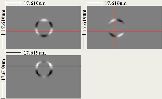
Further more, the discretization of convex structures like spheres easily causes aliasing effects we have to avoid. We cope with this problem by a Gaussian smoothing in radial direction. Figure 2.1 shows an example of a discrete base function template.

2.1.2 Band Limitation $b_{\max}$

Assuming that we obey the sampling theorem during the construction of $Y^{l}_{m}[r]$ (see previous section), we still have to worry about the effect of the band limitation of the harmonic expansion and reasonable choice of $b_{\max}$ below the theoretic limit.
The good news is that reconstructions from the harmonic domain are strictly band-wise operations (e.g. see (1.4)). Hence, the actual band limitation has no effect on the correctness of the lower frequencies: the band limitation simply acts as low-pass filter on the spherical signal. Figure 2.3³³ 3 Thanks to H. Skibbe for his volume rendering tool.shows the effects of the band-limitation in a synthetic example.

One should also keep in mind that a limitation of higher frequencies directly affects the angular resolution ${\cal SH}_{res}$ of the fast correlation and convolution in the harmonic domain (see section 1.4).

In the end, the selection of $b_{\max}$ is always a tradeoff between computational speed and maximum resolution.

2.1.3 Invariance

Another practical aspect of the harmonic expansion is that we are able to obtain additional invariance or robustness properties directly from the transformation implementation.

Gray-Scale Robustness

The most obvious example is the simple “trick” to become robust against gray-scale changes: As mentioned before in section 1.1, one very convenient property of the spherical harmonic transformations is that analogous to the Fourier transform, the constant component of the expanded signal is given by the 0th coefficient ${\cal SH}[r]\left(X\right)^{0}_{0}$ . Hence, we can easily achieve invariance towards shift of the mean gray-value in scalar operations if we simply normalize all coefficients by the 0th component.
Usually we denote this invariance only as “gray-scale robustness” since most practical applications include more complex gray-scale changes as this approach can handle.

Scale Normalization

It is also very easy to normalize the ${\cal SH}$ coefficients to compensate known changes in the scale of the data. In case we need to compute comparable features for data of different scale, we can normalize the coefficients ${\cal SH}[r]$ by the surface of the base functions, which is $4\pi r^{2}$ in a continuous setting. In the discrete case, we have to take the Gaussian smoothing into account: we simply use the sum over $Y_{0}^{0}$ as normalization coefficient.

Resolution Robustness

A typical problem which arises in the context of “real world” volume data is that we sometimes have to deal with non-cubic voxels, i.e. the input data is the result of a sampling of the real world which has not been equidistant in all spatial directions.
Such non-cubic voxels cause huge problems when we try to obtain rotation invariant features. Fortunately, we can cope with this problem during the construction of the base function templates $Y^{l}_{m}[r]$ : as figure 2.4 shows, we simply adapt the voxel resolution of the input data to the templates. Usually, we can obtain the necessary voxel resolution information directly from the imaging device.

2.1.4 Complexity

Concerning the voxel-wise local transformation for a single radius ${\cal SH}[r]\left(X\right)$ of a 3D volume $X$ with $m$ voxels, we obtain the harmonic expansion to band $b_{\max}$ in $O(m(b_{\max})^{2}+(m\log m))$ if we follow the fast convolution approach ( 2.3) and assume the base function templates are given.
Since we have to extract $n=b_{\max}(b_{\max}-1)$ coefficients, the memory consumption lies in $O(m(b_{\max})^{2})$ .

2.1.5 Parallelization

Further speed-up can be achieved by parallelization (see section 2.3): the data can be transformed into the harmonic domain by parallel computation of the coefficients. For ${\cal C}$ CPU cores with ${\cal C}\leq(b_{\max})^{2}$ and ${\cal C}\leq m$ we obtain: $O(\frac{m(b_{\max})^{2}}{\cal C})+O(\frac{(m\log m)}{\cal C})$ .

2.1.6 Fast Spherical Harmonic Transform

Recently, there has been an approach towards a fast Spherical Harmonic transform (fSHT) [16] for discrete signals. The fSHT uses a similar approach as in the FFT speed-up of the DFT and performs the computation of the entire inverse transformation in $O(N\log^{2}N)$ , where $N$ is the number of sampling points.
Since we hardly need the inverse transformation and only a small set of different extraction radii throughout this work, we prefer a simple caching of the pre-computed base functions to achieve faster transformations over of the quite complex fSHT method. Additionally, for real valued input data, we can exploit the symmetry properties ():

\overline{Y^{l}_{m}}=(-1)^{m}Y^{l}_{-m},

(2.4)

allowing us to actually compute only the positive half of the harmonic coefficients.

2.2 Discrete Vectorial Harmonic Transform

For the extraction of features on 3D vector fields, we need a discrete version of the Vectorial Harmonic transform (see section 1.6), i.e. we need to obtain the frequency decomposition of 3D vectorial signals at discrete positions on the discrete spherical neighborhoods ${{\cal S}[r]({\bf x})}$ (12) in ${\bf X}:\mathbb{Z}^{3}\rightarrow\mathbb{R}^{3}$ .
As for the discrete Spherical Harmonic transform, we pre-compute discrete approximations of the orthonormal harmonic base functions ${\bf Z}^{l}_{k,m}[r,{\bf x}]$ (1.64) which are centered in $\bf x$ . In their discrete version, the ${\bf Z}^{l}_{k,m}$ are parameterized in Euclidean coordinates ${\bf x}\in\mathbb{Z}^{3}$ rather then Euler angles:

{\cal VH}\big({\bf X}|_{{\cal S}[r]({\bf x})}\big)^{l}_{k,m}:=\sum\limits_{{\bf x_{i}}\in{\cal S}[r]({\bf x})}X({\bf x_{i}}){\bf Z}^{l}_{k,m}[r,{\bf x}]({\bf x_{i}}).

(2.5)

For most practical applications we have to compute the harmonic transformation of the neighborhoods around each voxel ${\bf x}$ , which can be computed very efficiently: since (2.6) is actually determined via convolution, we can apply the standard convolution theorem “trick” and perform a fast convolution via FFT to obtain ${\cal VH}^{l}_{k,m}({\bf X}):\mathbb{R}^{3}\rightarrow\mathbb{C}^{b}$ :

{\cal VH}[r]\left({\bf X}\right)^{l}_{k,m}={\bf X}*{\bf Z}^{l}_{k,m}[r].

(2.6)

The sampling and non-cubic voxel problems can be solved in the very same way as for the Spherical Harmonics. Figure 2.6 shows an artificial reconstruction example.
The complexity of a vectorial transformation grows by factor three compared to the Spherical Harmonics, but we are able to apply the same parallelization techniques.

2.2.1 Gray-Scale Invariance

The notion of gray-scale invariance might appear a bit odd, since vector fields are not directly associated with scalar gray values. But it is common practice to obtain the 3D vector fields by the gradient evaluation of 3D scalar data (see part III). Hence, it is of major interest to know if and how a 3D gradient vector field changes under gray-scale changes of the underlying data.
[33] showed that the gradient direction is in fact invariant under additive and multiplicative gray-scale changes. Therefore, we consider features based on Vectorial Harmonics to be gray-scale invariant - which is an important property for many applications.

2.3 Parallelization

Modern computing architectures come with an increasing number of general computing units: standard PCs have multi-core CPUs and more specialized computing servers combine several of these multi-core CPUs in a single system. This endorses the use of parallel algorithms.
In this work, parallel computing is only a little side aspect - but one with great speed-up potential. We restrict ourself to very simple cases of parallelization algorithms: first, we only consider systems with shared memory where all computing units (we refer to them as cores) share the same memory address space of a single system - hence, we explicitly disregard clusters. Second, we only consider algorithmically very simple cases of parallelization where the individual threads run independently, i.e. we avoid scenarios which would require a mutual exclusion handling, while still going beyond simplest cases data parallelization.
We give more details on the actual parallelization at the individual description of each feature implementation.

Chapter 3 ${\cal SH}$ -Features

In this chapter, we derive a set of local, rotation invariant features which are directly motivated by the sound mathematical foundation for operations on the 2-sphere introduced in chapter 1. We take advantage of the nice properties of Spherical Harmonics (1.2) which allow us to perform fast feature computations in the frequency domain.

Given scalar 3D volume data $X$ , the transformation ${\cal SH}\big(X|_{S[r]({\bf x})}\big)$ (2.2) of local data on a sphere with radius $r$ around the center point ${\bf x}$ in Spherical Harmonics is nothing more than a change of the base-functions representing the initial data. So the new base might provide us with a nice framework to operate on spheres, but we still have to perform the actual feature construction. Primarily, we want to obtain rotation and possibly gray-scale invariance.

First we introduce a simple method to obtain rotational invariance: In section 3.1 we review ${\cal SH}_{abs}$ features, which use the fact that the band-wise energies of a ${\cal SH}$ representation does not change under rotation. This method is well known from literature (i.e. [20]), but has its limitations.

To cope with some of the problems with ${\cal SH}_{abs}$ features, we introduced a novel rotation and gray-scale invariant feature based on the ${\cal SH}$ phase information [10]. We derive the ${\cal SH}_{phase}$ feature in section 3.2.

The third member of the ${\cal SH}$ -Feature class is a fast and also rotation invariant auto-correlation feature ${\cal SH}_{autocorr}$ (section 3.3) which is based on the fast correlation in Spherical Harmonics from section 1.4.

Finally, in section 3.4, we derive a complete local rotation invariant 3D feature from a global 2D image feature introduced in [21]. The ${\cal SH}_{bispectrum}$ feature.

3.1 ${\cal SH}_{abs}$

The feature we chose to call ${\cal SH}_{abs}$ throughout this work is also known as “Spherical Harmonic Descriptor” and has been used by several previous publications e.g. for 3D shape retrieval in [20]. We use ${\cal SH}_{abs}$ as one of our reference features to evaluate the properties and performance of our methods (see chapter 7).

3.1.1 Feature Design

${\cal SH}_{abs}$ achieves rotation invariance by exploiting some basic principals of the Spherical Harmonic (1.2) formulation. Analogous to the Fourier transformation, where we can use the power spectrum as a feature, we use the absolute values of each harmonic expansion band $l$ as power of the $l$ -th frequency in the Spherical Harmonic power spectrum:

\big({\cal SH}_{abs}[r]({\bf x})\big)^{l}:=\sqrt{\sum\limits_{m=-l}^{l}\left(\left({\cal SH}\big(X|_{S[r]({\bf x})}\big)\right)^{l}_{m}\right)^{2}}.

(3.1)

Rotation Invariance

Rotations ${\cal R(\phi,\theta,\psi)}\in{\cal SO}(3)$ (see section 1.2) are represented in the harmonic domain in terms of band-wise multiplications of the expansions $\widehat{f^{l}}$ with the orthonormal Wigner D-Matrices $D^{l}$ (1.19).
The power spectrum of a signal $f$ in Spherical Harmonics is given as (also see section 3.4 for more details):

q(f,l):=\big(\overline{\widehat{f^{l}}}\big)^{T}\widehat{f^{l}}.

(3.2)

The $D^{l}$ are orthonormal (1.25), hence it is easy to show the rotation invariance of the band-wise ${\cal SH}_{abs}$ entries of the power spectrum:

\displaystyle\begin{tabular}[]{r@{~ ~}lr }${\cal SH}_{abs}\big(D^{l}({\cal R})\widehat{f^{l}}\big)$\penalty\ \penalty\ &$=\big(\overline{D^{l}({\cal R})\widehat{f^{l}}}\big)^{T}D^{l}({\cal R})\widehat{f^{l}}$&\\[3.55658pt] \penalty\ \penalty\ &$=\big(\overline{\widehat{f^{l}}}\big)^{T}\big(\overline{D^{l}({\cal R})}\big)^{T}D^{l}({\cal R})\widehat{f^{l}}$&\\[3.55658pt] \penalty\ \penalty\ &$=\big(\overline{\widehat{f^{l}}}\big)^{T}\widehat{f^{l}}$&\end{tabular}.

So, we note that a rotation has only a band-wise effect on the expansion but does not change the respective absolute values. Hence, the approximation of the original data via harmonic expansion can be cut off at an arbitrary band, encoding just the level of detail needed for the application.

Gray-Scale Robustness:

We can obtain invariance towards additive gray-scale changes by normalization by the $0$ th harmonic coefficient as described in section 2.

3.1.2 Implementation

The implementation of the ${\cal SH}_{abs}$ is straightforward. We follow the implementation of the Spherical Harmonic transformation as described in chapter 2.

Multi-Channel Data:

${\cal SH}_{abs}$ cannot directly combine data from several channels into a single feature. In case of multi-channel data, we have to separately compute features for each channel.

Complexity

Following the implementation given in section 2, we obtain the harmonic expansion to band $b_{\max}$ at each point of a volume with $m$ voxels in $O(m(b_{\max})^{2}+(m\log m))$ . The computation of the absolute values takes another $O((b_{\max})^{3})$ .

Parallelization

Further speed-up can be achieved by parallelization (see section 2): the data can be transformed into the harmonic domain by parallel computation of the coefficients and the computation of the absolute values can also be split into several threads. For ${\cal C}$ CPU cores with ${\cal C}\leq(b_{\max})^{2}$ and ${\cal C}\leq m$ we obtain:

O(\frac{m(b_{\max})^{3}}{\cal C})+O(\frac{m(b_{\max})^{2}+(m\log m)}{\cal C})

3.1.3 Discussion

The ${\cal SH}$ -Features are a simple and straightforward approach towards local 3D rotation invariant features. They are computationally efficient and easy to implement, however, the discriminative properties are quite limited. The band-wise absolute values only capture the energy of the respective frequencies in the overall spectrum. Hence, we loose all the phase information which leads to strong ambiguities within the feature mappings. In many applications it is possible to reduce these ambiguities by the combination of ${\cal SH}$ -Features which were extracted at different radii.

${\cal SH}_{abs}$ Ambiguities:

in theory, there is an infinite number of input patterns which are mapped on the same ${\cal SH}$ -Feature just as there is an infinite number of possible phase shifts in harmonic expansions. However, one might argue that this does not prevent a practically usage of the ${\cal SH}$ -Feature since we generally do not need completeness (see section 0.2.2).
But we still need discriminative features, and there are practical relevant problems where ${\cal SH}_{abs}$ is not powerful enough, as figure 3.1 shows.

3.2 ${\cal SH}_{phase}$

Motivated by the ambiguity problems caused by neglecting the phase information in the ${\cal SH}_{abs}$ -Features (see discussion in section 3.1.3) we presented an oppositional approach in [10]. ${\cal SH}_{phase}$ -Features preserve only the phase information of the Spherical Harmonic representation and disregard the amplitudes. This approach is further motivated by results known from Fourier transform, which showed that the characteristic information is dominant in the phase of a signal’s spectrum rather than in the pure magnitude of it’s coefficients [24]. Following a phase-only strategy has the nice side-effect that since the overall gray-value intensity is only encoded in the amplitude, the ${\cal SH}_{phase}$ method is gray-scale invariant. Like the ${\cal SH}_{abs}$ -Features (from section 3.1) ${\cal SH}_{phase}$ -Features are computed band-wise, but instead of a single radius ${\cal SH}_{phase}$ combines expansions at different radii $r_{1},r_{2}$ into a feature.

3.2.1 Feature Design

The phase of a local harmonic expansion in band $l$ at radius $r$ is given by the orientation of the vector ${\bf p}^{l}[r]$ , which contains the $2l+1$ harmonic coefficient components of the band-wise local expansion (3.7). Since the coefficients are changing when the underlying data is rotated, the phase itself is not a rotational invariant feature.

{\bf p}^{l}_{m}[r]\left({\bf x}\right):=\frac{\left({\cal SH}\big(X|_{S[r]({\bf x})}\big)\right)^{l}_{m}}{\big({\cal SH}_{abs}[r]\left({\bf x}\right)\big)^{l}}

(3.7)

Since we are often interested in encoding the neighborhood at several concentric radii, we can take advantage of this additional information and construct a phase-only rotational invariant feature based on the band-wise relations of phases between the different concentric harmonic series.
Fig. (3.2) illustrates the basic idea: for a fixed band $l$ , the relation (angle) between phases of harmonic expansions at different radii are invariant towards rotation. Phases in the same harmonic band undergo the same changes under rotation of the underlying data (see section 1.2 for details), keeping the angle between the phases of different radii constant. We encode this angle in terms of the dot-product of band-wise Spherical Harmonic expansions at radii $r_{1},r_{2}$ :

\left({\cal SH}_{phase}[r_{1},r_{2}]\left({\bf x}\right)\right)^{l}:=\langle{\bf p}^{l}[r_{1}],{\bf p}^{l}[r_{2}]\rangle.

(3.8)

Rotation Invariance:

the proof of the rotation invariance is rather straightforward basic linear algebra:

\displaystyle\begin{tabular}[]{r@{~ ~}lr }Rotations ${\cal R}X$ acting on \ref{eq:feature:SHphase}:\penalty\ \penalty\ &$\langle D^{l}{\bf p}^{l}[r_{1}],D^{l}{\bf p}^{l}[r_{2}]\rangle$&\\[3.55658pt] \penalty\ \penalty\ &$=\big(\overline{D^{l}{\bf p}^{l}[r_{1}]}\big)^{T}(D^{l}{\bf p}^{l}[r_{2}])$&rewrite as matrix multiplication\\[3.55658pt] \penalty\ \penalty\ &$=\big(\overline{{\bf p}^{l}[r_{1}]}\big)^{T}(\overline{D^{l}})^{T}(D^{l}{\bf p}^{l}[r_{2}])$&resolve transposition\\[3.55658pt] \penalty\ \penalty\ &$=\big(\overline{{\bf p}^{l}[r_{1}]}\big)^{T}\left((\overline{D^{l}})^{T}D^{l}\right)({\bf p}^{l}[r_{2}])$&commutativity\\[3.55658pt] \penalty\ \penalty\ &$=\big(\overline{{\bf p}^{l}[r_{1}]}\big)^{T}\underbrace{\left((\overline{D^{l}})^{T}D^{l}\right)}_{=I}({\bf p}^{l}[r_{2}])$&use orthogonality of $D^{l}$\\[3.55658pt] \penalty\ \penalty\ &$=\big((\overline{{\bf p}^{l}[r_{1}]})^{T}{\bf p}^{l}[r_{2}]\big)$&\\[3.55658pt] \penalty\ \penalty\ &$=\langle{\bf p}^{l}[r_{1}],{\bf p}^{l}[r_{2}]\rangle$&\end{tabular}.

The rotation ${\cal R}$ of the underlying data can now be expressed in terms of matrix multiplications with the same Wigner-D matrix $D^{l}$ (1.19). Since the rotational invariance is achieved band-wise, the approximation of the original data via harmonic expansion can be cut off at an arbitrary band, encoding just the level of detail needed for the application.

3.2.2 Implementation

The implementation of the ${\cal SH}_{phase}$ is straightforward. We follow the implementation of the Spherical Harmonic transformation as described in section 2 for the two radii $r_{1}$ and $r_{2}$ . The band-wise computation of the phases and the evaluation of the dot-product is also very simple.

Multi-Channel Data:

${\cal SH}_{phase}$ -Features can also directly combine data from several channels into a single feature: we simply extract the harmonic expansions for the different radii from different data channels.

Complexity

Following the implementation given in section 2, we obtain the harmonic expansion to band $b_{\max}$ at each point of a volume with $m$ voxels in $O(m(b_{\max})^{2}+(m\log m))$ . The computation of the dot-products and the phase vectors takes another $O((b_{\max})^{3})$ .

Parallelization

Further speed-up can be achieved by parallelization (see section 2.3): the data can be transformed into the harmonic domain by parallel computation of the coefficients and the computation of the absolute values can also be split into several threads. For ${\cal C}$ CPU cores with ${\cal C}\leq(b_{\max})^{2}$ and ${\cal C}\leq m$ we obtain:

O(\frac{m(b_{\max})^{3}}{\cal C})+O(\frac{m(b_{\max})^{2}+(m\log m)}{\cal C})

3.2.3 Discussion

Event though the ${\cal SH}_{phase}$ -Features are not complete either, their discrimination abilities tend to be better than those of the ${\cal SH}_{abs}$ -Features (see section 3.1). Also, the additional gray-scale invariance is very useful in many applications.
Intuitively, ${\cal SH}_{phase}$ encodes local changes between the different radii. This property is especially applicable for texture classification or to find 3D interest points (see part III).

3.3 ${\cal SH}_{autocorr}$

The next approach to compute invariant features directly from the harmonic representation is motivated by the introduction of the fast normalized cross-correlation in the harmonic domain (see introduction of chapter 1.4). The cross-correlation ${\cal SH}_{corr}(f,g)$ on two signals $f,g\in S^{2}$ is a binary operation ${\cal SH}_{corr}:S^{2}\times S^{2}\rightarrow\mathbb{R}$ . Hence, it cannot be used directly as a feature, where we require a mapping of individual local signals $f\in S^{2}\rightarrow{\cal H}$ into some feature space ${\cal H}\subseteq\mathbb{R}^{n}$ (see section Introduction and Perquisites).
A general and widely known method to obtain features from correlations is to compute the auto-correlation, e.g. [19]. In our case, we propose the local ${\cal SH}_{autocorr}$ -Feature, which performs a fast auto-correlation of $f\in S^{2}$ .

The auto-correlation under a given rotation $\cal R$ in Euler angles $\phi,\theta,\psi$ is defined as:

(f\#f)({\cal R}):=\int\limits_{S^{2}}f({\cal R}f)\text{\quad}\sin{\Theta}d\Phi d\Theta.

(3.17)

3.3.1 Feature Design

As for most of our other features, we first expand the local neighborhood $f$ at radius $r$ around the point ${\bf x}$ in Spherical Harmonics, $\widehat{f}:={\cal SH}\big(X|_{S[r]({\bf x})}\big)$ .
Then we follow the fast correlation method which we introduced in section 1.4 to obtain the full correlation $C^{\#}$ from equation (1.45).

Invariance:

In order to obtain rotation invariant features, we follow the Haar-Integration approach (see chapter 4.0.1) and integrate over the auto-correlations at all possible rotations $\cal R$ . $C^{\#}$ holds the necessary auto-correlation results in a 3D $(\phi,\theta,\psi)$ -space (1.44), hence we simply integrate over $C^{\#}$ ,

{\cal SH}_{autocorr}:=\int\limits_{\phi,\theta,\psi}\kappa\left(C^{\#}(\phi,\theta,\psi)\right)\sin{\theta}d\phi d\theta d\psi

(3.18)

and obtain a scalar feature. Additionally, we insert a non-linear kernel function $\kappa$ to increase the separability. Usually, very simple non-linear functions, such as $\kappa(x):=x^{2},\kappa(x):=x^{3}$ or $\kappa(x):=\sqrt{x}$ , are sufficient.

Like in the case of the ${\cal SH}_{abs}$ -Features, we can obtain invariance towards additive gray-scale changes by normalization by the $0$ th harmonic coefficient. If we additionally normalize $C^{\#}$ as in (1.57), ${\cal SH}_{autocorr}$ becomes completely gray-scale invariant.

3.3.2 Implementation

We follow the implementation of the Spherical Harmonic transformation as described in chapter 2 and the implementation of the fast correlation from (1.53).
In practice, where the harmonic expansion is bound by a maximal expansion band $b_{\max}$ , the integral (3.18) is reduce to the sum over the then discrete angular space $C^{\#}$ :

{\cal SH}_{autocorr}=\sum\limits_{\phi,\theta,\psi}\kappa\left(C^{\#}(\phi,\theta,\psi)\right).

(3.19)

Multi-Channel Data:

It is straightforward to combine the information from several data channels into a single ${\cal SH}_{autocorr}$ -Feature: We simply use the same approach as described in section 1.4.6, where we correlated the information of several different radii.

Complexity

Following the implementation given in chapter 2, we obtain the harmonic expansion to band $b_{\max}$ at each point of a volume with $m$ voxels in $O(m(b_{\max})^{2}+(m\log m))$ . The complexity of the auto-correlation depends on $b_{\max}$ and the padding parameter $p$ (1.53) and can be computed in $O(m(b_{\max}+p)^{3}\log(b_{\max}+p)^{3}))$ . The sum over $C^{\#}$ takes another $O((b_{\max}+p)^{3})$ at each point.

Parallelization:

Further speed-up can be achieved by parallelization (see section 2): the data can be transformed into the harmonic domain by parallel computation of the coefficients and the computation of the absolute values also be split into several threads. For ${\cal C}$ CPU cores with ${\cal C}\leq(b_{\max})^{2}$ and ${\cal C}\leq m$ we obtain:

O(\frac{m\left((b_{\max}+p)^{3}+(b_{\max}+p)^{3}\log(b_{\max}+p)^{3}\right)}{\cal C})+O(\frac{m(b_{\max})^{2}+(m\log m)}{\cal C})

3.3.3 Discussion

Auto-correlation can be a very effective feature to encode texture properties. The discriminative power of ${\cal SH}_{autocorr}$ can be further increased by we combining the correlation a several different radii to a single correlation result $C^{\#}$ , as described in section 1.4.

3.4 ${\cal SH}_{bispectrum}$

The final member of the class of features which are directly derived from the Spherical Harmonic representation is the so-called ${\cal SH}_{bispectrum}$ -Feature. The approach to obtain invariant features via the computation of the bispectrum of the frequency representation is well known (e.g. see [48]), hence, we review the basic concept in a simple 1D setting before we move on to derive it in Spherical Harmonics.

Given a discrete complex 1D signal $f:\{0,1,\dots,n-1\}\rightarrow\mathbb{C}$ and its DFT $\widehat{f}$ , the power spectrum $q(f,\omega)$ of $f$ at frequency $\omega$ is:

q(f,\omega):=\overline{\widehat{f}(\omega)}\cdot\widehat{f}(\omega).

(3.20)

The power spectrum is translation invariant since a translation $z$ of $f$ only affects the phases of the Fourier coefficients which are canceled out by $\overline{\widehat{f}(\omega)}\cdot\widehat{f}(\omega)$ :

	$\displaystyle\overline{e^{-i2\pi z\omega/n}\widehat{f}(\omega)}\cdot e^{-i2\pi z\omega/n}\widehat{f}(\omega)$	$\displaystyle=$	$\displaystyle e^{i2\pi z\omega/n}\overline{\widehat{f}(\omega)}\cdot e^{-i2\pi z\omega/n}\widehat{f}(\omega)$		(3.21)
		$\displaystyle=$	$\displaystyle\overline{\widehat{f}(\omega)}\cdot\widehat{f}(\omega).$		(3.22)

We use the same principle to construct the ${\cal SH}_{abs}$ -Features (see section 3.1). As mentioned in the context of ${\cal SH}_{abs}$ , neglecting the valuable phase information makes the power spectrum not a very discriminative feature.
The basic idea of the bispectrum is to couple two frequencies $\omega_{1},\omega_{2}$ in order to implicitly preserve the phase information:

q(f,\omega_{1},\omega_{2}):=\overline{\widehat{f}(\omega_{1})}\cdot\overline{\widehat{f}(\omega_{2})}\cdot\widehat{f}(\omega_{1}+\omega_{2}).

(3.23)

While the invariance property is the same as for the power spectrum:

\displaystyle e^{i2\pi z\omega_{1}/n}\overline{\widehat{f}(\omega_{1})}\cdot e^{i2\pi z\omega_{2}/n}\overline{\widehat{f}(\omega_{2})}\cdot e^{-i2\pi z(\omega_{1}+\omega_{2})/n}\widehat{f}(\omega_{1}+\omega_{2})=\overline{\widehat{f}(\omega_{1})}\cdot\overline{\widehat{f}(\omega_{2})}\cdot\widehat{f}(\omega_{1}+\omega_{2}),

(3.24)

it has been shown [48] that the phases $\omega_{i}$ can be reconstructed from the bispectra. Hence, the bispectrum is a complete feature if $f$ is band limited and we extract the bispectrum at all frequencies.

Due to the analogy of the Spherical Harmonic and the Fourier domain, it is intuitive that the concept of the bispectrum is portable to signals in $S^{2}$ . This step was derived by [21] who constructed a global invariant feature for 2D images by projecting the images on the 2-sphere and then computing features in the harmonic domain. We adapt the methods from [21] to construct local rotation invariant features for 3D volume data.

3.4.1 Feature Design

In our case, we are interested in the extraction of invariant features of the local neighborhood $f$ at radius $r$ around the point ${\bf x}$ . Just as in the 1D example, we transform $f$ into the frequency space - i.e. in the Spherical Harmonic domain: $\widehat{f}:={\cal SH}\big(X|_{S[r]({\bf x})}\big)$ .
Now, the individual frequencies $\omega$ correspond to the harmonic bands $\widehat{f}^{l}$ , and [21] showed that the bispectrum can be computed from the tensor product $(\widehat{f})^{l_{1}}\otimes(\widehat{f})^{l_{2}}$ .
Further, we want to obtain invariance towards rotation instead of translation: given rotations ${\cal R}\in{\cal SO}(3)$ , the tensor product is affected by ${\cal R}$ in terms of:

{\cal R}\left((\widehat{f})^{l_{1}}\otimes(\widehat{f})^{l_{2}}\right)=\left(D^{l_{1}}({\cal R})\otimes D^{l_{2}}({\cal R})\right)\left((\widehat{f})^{l_{1}}\otimes(\widehat{f})^{l_{2}}\right),

(3.25)

where $D^{l}$ is the Wigner-D matrix for the $l$ -th band (see section 1.2).
Just like in the 1D case, [21] proved that the bispectrum (3.25) will cancel out the impact of the rotation $\cal R$ . So, for the $l$ -th band of expansion we can compute the bispectrum of the $l_{1}$ -th and $l_{2}$ -th band with $l_{1},l_{2}\leq l$ by:

\left({\cal SH}_{bispectrum}\right)^{l_{1},l_{2},l}:=\sum\limits_{m=-l}^{l}\sum\limits_{m_{1}=-l_{1}}^{l_{1}}\langle lm|l_{1}m_{1},l_{2}m_{2}\rangle\overline{\widehat{f}^{l_{1}}_{m_{1}}}\cdot\overline{\widehat{f}^{l_{2}}_{(m-m_{1})}}\cdot\widehat{f}^{l}_{m},

(3.26)

where the Clebsch-Gordan coefficients (see section 1.3) $\langle lm|l_{1}m_{1},l_{2}m_{2}\rangle$ determine the impact of the frequency couplings in the tensor product computing the bispectrum. Refer to [21] for full proof.

3.4.2 Implementation

As before, we follow the implementation of the Spherical Harmonic transformation as described in chapter 2 and stop the expansion at an arbitrary band $b_{\max}$ (depending on the application) which has no effect on the rotation invariance.
The actual computation of bispectrum from (3.26) can be optimized by removing the $\widehat{f}^{l}_{m}$ term to the outer iteration and limiting the inner iteration to values which form possible Clebsh-Gordan combinations:

\left({\cal SH}_{bispectrum}\right)^{l_{1},l_{2},l}=\sum\limits_{m=-l}^{l}\widehat{f}^{l}_{m}\times\sum\limits_{m_{1}=\max{-l_{1},(m-l_{2})}}^{\min{l_{1},(m+l_{2})}}\langle lm|l_{1}m_{1},l_{2}m_{2}\rangle\overline{\widehat{f}^{l_{1}}_{m_{1}}}\cdot\overline{\widehat{f}^{l_{2}}_{(m-m_{1})}}.

(3.27)

Multi-Channel Data:

It is straightforward to combine the information from two different data channels into a single ${\cal SH}_{bispectrum}$ -Feature: we can simply choose the coefficients $\widehat{f}^{l_{1}}$ and $\widehat{f}^{l_{2}}$ from two t expansions of the data from two different channels.

Complexity

The computational complexity of a singe $\left({\cal SH}_{bispectrum}\right)^{l_{1},l_{2},l}({\bf x})$ feature lies in $O(l^{3})$ . To obtain completeness we need all $O(b_{\max}^{2})$ features at all $m$ positions of $X$ . The harmonic expansion to band $b_{\max}$ at each point takes another $O(m(b_{\max})^{2}+(m\log m))$ .

Parallelization

It is straightforward to get further speed-up by parallelization (see chapter 2). Since the computation of each single feature $\left({\cal SH}_{bispectrum}\right)^{l_{1},l_{2},l}({\bf x})$ is independent from all others, we can split the overall process in parallel computations.

3.4.3 Discussion

The basic concept of the ${\cal SH}_{bispectrum}$ -Features is quite similar to what we did for the ${\cal SH}_{phase}$ -Features (see section 3.2): we try to obtain a better discrimination performance than ${\cal SH}_{abs}$ -Features by implicit preservation of the phase information. In case of the ${\cal SH}_{phase}$ -Features we do this by considering the relation of phases over different radii of the expansion, here we relate different frequencies of the expansion. In theory, the completeness property makes the ${\cal SH}_{bispectrum}$ approach very competitive, but this comes at high computational costs.

Chapter 4 Scalar Haar-Features

In this chapter we derive several features operating on scalar data which obtain invariance via Haar-Integration. As discussed in section 0.2.2, one canonical approach to construct invariant features is to perform a Haar-Integration over the transformation group.
Before we turn to the specific feature design, we first review the general framework of Haar-Integration in section 4.0.1 and discuss some aspects of the construction of suitable feature kernels in section 4.0.2. Then we introduce $2p$ -Haar features 4.1 and $3p$ -Haar features 4.2 which are based on the class of separable kernel functions, before we derive the generalized $np$ -Haar features.

It should be noted that we also use Haar-Integration methods for the computation of the auto-correlation features ${\cal SH}_{autocorr}$ (see section 3.3) and ${\cal VH}_{autocorr}$ (see section 5.2).

Related Work:

Based on the general group-integration framework (4.2) which was introduced by [44], [45] and [5], several invariant features were introduced for scalar data in 2D [45] and in 3D volumetric data [39] [34] [35] [13]. We will discuss these methods in the next section when we take a closer look at the class of sparse and separable kernels [34] [35] [13] which form the basis of our features.

4.0.1 Invariance via Group-Integration

Following the general objectives of feature extraction (see 0.2.1) we apply the Haar-Intergration approach to obtain invariant features. This method is generally bound to the sub-class of compact group transformations (see 0.2.2), where for a given transformation group ${\cal G}$ , the individual transformations $g\in{\cal G}$ differ only by their associated set of parameters $\boldsymbol{\mathbf{\lambda}}$ , which cover the degrees of freedom under ${\cal G}$ .

In this chapter we derive features from the canonical group integration approach (see section 0.2.2) which generates invariant features via Haar-Integration over all degrees of freedom of the transformation group $G$ :

T(X)=\int\limits_{\cal G}(g_{\boldsymbol{\mathbf{\lambda}}}{X})dg_{\boldsymbol{\mathbf{\lambda}}},

(4.1)

eliminating the influence of $\boldsymbol{\mathbf{\lambda}}$ . Equation (4.1) is also referred to as the “group-average”. For the cause of simplicity, we denote individual transformation $g_{\boldsymbol{\mathbf{\lambda}}}$ just by $g$ .

It has to be noted that even though the Haar-Integration approach (4.1) meets the necessary condition of invariance (7), the sufficient condition (8) is anything but guaranteed. In fact, a simple group-averaging itself produces incomplete features which often tend to have a weak separability performance. This can be overcome by embedding non-linear kernel functions $\kappa$ into the integral [44]: it cannot be stressed enough that the use of such non-linear mappings is essential for any feature design [4] [44] [45] [34] [13], and is the key element of the group-integration framework. The resulting general framework for invariant feature generation via group-integration (4.2) then embeds an arbitrary non-linear kernel function $\kappa$ .

\displaystyle T(X):=\int\limits_{\cal G}\kappa(g{X})dg

(4.2)

${\cal G}$ :	transformation group
$g$ :	one element of the transformation group
$dg$ :	Haar measure
$\kappa$ :	nonlinear kernel function
${X}$ :	$n$ -dim, multi-channel data set
$g{X}$ :	the transformed $n$ -dim data set

Within this framework, features can be generated for data of arbitrary dimensionality and from multiple input channels. This reduces the key design issue to the selection of appropriate kernel functions.

4.0.2 Local, Sparse and Separable Kernel Functions

Since we are interested in the construction of local features, we restrict the kernel functions $\kappa$ in the general group-integration approach (4.2) to functions of local support.

Further, following the approach in [34] [13], we restrict these local kernels to sparse functions which only depend on a few discrete points of the local continuous data. Hence, $\kappa({X})$ can be rewritten as $\kappa\left({X}({\bf x}_{1}),{X}({\bf x}_{2}),{X}({\bf x}_{3}),\dots\right)$ [13].
This way, we can reformulate (4.2) and perform the group transformation only on the local kernel support, instead of the whole data set ${X}$ (see Fig. 4.1). This local transformation is denoted as $s_{g}({\bf x}_{i})$ such that

(g{X})({\bf x}_{i})=:{X}(s_{g}({\bf x}_{i}))\quad\forall g,{\bf x}_{i}.

(4.3)

For these local kernels, (4.2) can be rewritten as

\displaystyle T(X):=\int\limits_{G}\kappa\left({X}(s_{g}({\bf x}_{1})),\;{X}(s_{g}({\bf x}_{2})),\dots\right)dg.

(4.4)

Fig. (4.1) shows how a sparse kernel with a local support of three discrete points can be applied to “sense” the local continuous data.

For kernels with a larger support it does not make much sense to combine single data points over a certain distance. Instead we are interested in combining larger structures, i.e. in having a kernel over regions rather than over single points. One very simple way to achieve this was suggested in [34]: by applying a Gaussian smoothing of the input data which directly depends on the selected size of the local support, we can define a “multi-scale” kernel which has different sizes of local support in each point.

This class of local sparse kernel functions provides a more structured but still very flexible framework for the design of local invariant features. However, even with a support reduced to $n$ discrete points, naive kernel computation is still very expensive since the local support has to be integrated over the entire transformation group. [45][40][5] suggested to overcome this problem by the use of Monte Carlo methods, but this approach is only effective when features are computed via integration over the entire dataset (i.e. integration over the translation group). For the computation of local features, i.e. a Monte Carlo integration over the rotation group is not suitable.

To make group-integral features applicable to large data sets, [34] introduced a sub-class of sparse kernel-functions. For these so called separable kernels, the kernel can be split into a linear combination of non-linear sub-kernels such that:

\displaystyle\kappa\left({X}(s_{g}({\bf x}_{1})),\;{X}(s_{g}({\bf x}_{2})),\dots\right)=\kappa_{1}\left({X}(s_{g}({\bf x}_{1}))\right)\cdot\kappa_{2}\left({X}(s_{g}({\bf x}_{2}))\right)\cdot\dots.

(4.5)

This separability constraint is not a strong limitation of the original class of sparse kernel-functions since in many cases it is possible to find approximative decompositions of non-separable kernels via Taylor series expansion.
Besides the non-linearity, the choice of the sub-kernels $\kappa_{i}$ is theoretically not further constrained, but in most cases very simple non-linear mappings such as $\kappa(x)=x^{2},\kappa(x)=x^{3},\dots$ or $\kappa(x)=\sqrt{x}$ are powerful enough (see experiments in part III).

Based on these separable kernels, [34] derived a fast convolution method for the evaluation of kernels with a support of only two sparse points on continuous 2D images - so called “2-point” kernels (see section 4.1).

4.1 2-Point Haar-Features ( $2p$ )

Our first feature which makes use of the general group integration framework (4.2) is the so-called 2-Point or $2p$ -Haar feature. It was first introduced as a global feature for 2D images in [34]. We later extended this approach to local features on scalar 3D volume data in [35] and [36] with an application to biomedical 3D image analysis in [12] (see part III).

$2p$ -Features use a sub-class of the previously introduced separable kernel functions (4.5). The name 2-Point derives from the constraint that we restrict kernels to have just two separable kernel points ${\bf x}_{1},{\bf x}_{2}$ . This restriction allows a reformulation of the initial parameterization $\bf\lambda$ of the rotation group ${\cal SO}(3)$ , which is drastically reducing the computational complexity necessary to obtain rotation invariance. However, this comes at the price of reduced discrimination power as we discuss at the end of this section.

4.1.1 Feature Design

The selection of the kernel points ${\bf x}_{1}$ and ${\bf x}_{2}$ is bound by the following design principle for the 2-Point features: For the extraction of a local $2p$ -Feature at a given point ${\bf x}$ in $X$ of the scalar (or possibly multi-channel) 3D input volume $X$ , ${\bf x}_{1}$ is fixed at the center of the neighborhood, i.e. ${\bf x}_{1}:=X({\bf x})$ . The second kernel point is chosen from the local neighborhood: ${\bf x}_{2}\in S[r]\left({\bf x}\right)$ (see 12 for the neighborhood definition).
Since ${\bf x}_{1}$ is fixed, we only have to choose the parameters for ${\bf x}_{2}$ : the local neighborhood $r$ and the spherical coordinates $\Phi,\Theta$ which can be neglected later on.
We are using the scheme for separable kernels (4.5), we can write the $2p$ -Kernels as:

\kappa\big(X({\bf x}_{1}),X({\bf x}_{2})\big)=\kappa_{1}\big(X({\bf x}_{1})\big)\cdot\kappa_{2}\big(X({\bf x}_{2})\big).

(4.6)

Figure 4.2 shows a schematic example of a local 3D $2p$ kernel on volume data.

Rotation Invariance

As for all other local features, we want to obtain rotation invariance. If we plug the $2p$ kernel (4.6) into the general Haar framework (4.2), we can achieve invariance regarding rotations ${\cal R(\phi,\theta,\psi)}\in{\cal SO}(3)$ parameterized in Euler angles (see section 1.2) with local transformations (4.5) $s_{\cal R}(\phi,\theta,\psi)\in{\cal SO}(3)$ . Since ${\bf x}_{1}$ is by definition always in the rotation center, it is not affected by any rotation. Hence we can simplify the Haar-Integration for the multiplicative and separable $2p$ -Kernel functions:

T[r,{\bf x}_{2}]({\bf x}):=\kappa_{1}\big(X({\bf x})\big)\cdot\int\limits_{{\cal SO}(3)}\kappa_{2}\big(X(s_{\cal R(\phi,\theta,\psi)}({\bf x}_{2}))\big)\sin{\theta}d\phi d\theta d\psi.

(4.7)

Fast Computation

In order to compute (4.7) we have to evaluate the integral over all possible rotations at each point $X({\bf x})$ , which turns out to be quite expensive in terms of computational complexity. At this point, the restriction of (4.5) to two points provides us with a fast solution: due to the fact that we have to integrate only over the position of a single point ${\bf x}_{2}\in S[r]\left(X({\bf x})\right)$ , the integral over $\psi$ becomes a constant factor and we can rewrite (4.7) as:

T[r,{\bf x}_{2}]({\bf x})=\kappa_{1}\big(X({\bf x})\big)\cdot\int\limits_{\phi,\theta}\kappa_{2}\big(X(s_{\cal R(\phi,\theta,\psi)}({\bf x}_{2}))\big)\sin{\theta}d\phi d\theta.

(4.8)

Since ${\bf x}_{2}\in S[r]\left({\bf x}\right)$ is also parameterized in $\phi,\theta$ , we can further reformulate the integral and simply solve:

T[r,{\bf x}_{2}]({\bf x})=\kappa_{1}\big(X({\bf x})\big)\cdot\int\limits_{{\bf x_{i}}\in{\cal S}[r]({\bf x})}\kappa_{2}\big(X\big|_{{\cal S}[r]({\bf x})}({\bf x}_{i})\big).

(4.9)

Finally, the integration over a spherical neighborhood $S[r]\left({\bf x}\right)$ can easily be formulated as convolution of $X\big|_{{\cal S}[r]({\bf x})}$ with a spherical template $S_{t}[r]$ with $S_{t}[r](\Phi,\Theta)=1,\text{\quad}\forall\Phi\in[0,\dots,2\pi],\Theta\in[0,\dots,\pi]$ :

T[r]({\bf x})=\kappa_{1}\big(X({\bf x})\big)\cdot\big(\kappa_{2}(X\big|_{{\cal S}[r]({\bf x})})*S_{t}[r]({\bf x})\big).

(4.10)

In the same way, we can evaluate the $2p$ -Feature at all positions in $X$ at once, using fast convolution in the Fourier domain:

T[r](X)=\kappa_{1}(X)\cdot\big(\kappa_{2}(X)*S_{t}[r]\big).

(4.11)

4.1.2 Implementation

The implementation is straightforward: given discrete input data, we apply the convolution theorem to compute the convolution via FFT:

T[r](X)=\kappa_{1}(X)\cdot{FFT^{-1}}\big({FFT}(\kappa_{2}(X))\cdot{FFT}(S_{t}[r])\big).

(4.12)

The only thing we have to handle with some care is the implementation of the spherical template $S_{t}[r]$ . To avoid sampling issues, we apply the same implementation strategies as in the case of the Spherical Harmonic base functions (see section 2.1 for details).

Multi-Channel Data:

Naturally, the application of $2p$ -Features to multi-channel data is limited to two channels per feature, but this is straightforward: we can simply set the kernel points to be on different data channels $c_{i}$ :

T[r](X)=\kappa_{1}\big(X[c_{1}]\big)\cdot\big(\kappa_{2}(X[c_{2}]\big|_{{\cal S}[r]({\bf x})})*S_{t}[r]\big).

(4.13)

Complexity:

By reducing the feature computation to a fast convolution, we end up with a complexity of $O(m\log m)$ for an input volume with $m$ voxels.

Parallelization:

Since there is no easy way to parallelize the Fourier Transformation, we do not further parallelize the computation of $2p$ -Features. However, because $2p$ -Features can be computed so fast anyway, this is not a real drawback.

4.1.3 Discussion

The best property of $2p$ -Features is their computational speed: no other spherical local 3D feature, neither in the context of this work nor in the literature can be computed this fast. However, the speed comes at the price of a rather low discrimination power and the lack of gray-scale robustness. While one might try to compensate the missing gray-scale robustness by pre-normalization of the input data, the discrimination power hardly can be improved.
The problem is caused by the fact that $2p$ -Features are not only invariant under rotations, but also under arbitrary permutations of signals on the sphere. This causes problematic ambiguities, as illustrated in figure 4.3.

4.2 3-Point Haar-Features ( $3p$ )

3-Point Haar-Features (or $3p$ -Features) are a direct extension of separable kernels (4.5) from two (4.6) to three kernel points. The main motivation for this extension derives from the discussion of the $2p$ -Features (see section 4.1.3), where we pointed out that even though 2-point kernels (4.6) provide computationally very efficient features, the resulting discrimination power is flawed by the fact that these kernels are also invariant to arbitrary permutations.
To overcome this major drawback, we introduced the $3p$ -Features in [35] and [13]. The basic idea is to add a third kernel point ${\bf x}_{3}$ to the separable kernel function $\kappa$ (4.5) (see figure 4.5), which cancels out the permutation ambiguities:

\kappa\big(X({\bf x}_{1}),X({\bf x}_{2}),X({\bf x}_{3})\big)=\kappa_{1}\big(X({\bf x}_{1})\big)\cdot\kappa_{2}\big(X({\bf x}_{2})\big)\cdot\kappa_{3}\big(X({\bf x}_{3})\big).

(4.14)

4.2.1 Feature Design

As in the $2p$ case, we fix the first kernel point ${\bf x}_{1}:=X({\bf x})$ at the point of the local feature extraction, while the other two points are placed at the concentric spherical neighborhoods surrounding the first point: ${\bf x}_{2}\in S[r_{2}]\left({\bf x}\right),{\bf x}_{3}\in S[r_{3}]\left({\bf x}\right)$ .
Of course, both kernel points ${\bf x}_{2},{\bf x}_{3}$ can be on the same sphere, resulting in $r_{2}=r_{3}$ , and are parameterized in spherical coordinates $\Phi_{2},\Phi_{3}$ and $\Theta_{2},\Theta_{3}$ . Figure 4.6 shows examples of such $3p$ -Kernels.

Rotation Invariance

If we plug the $3p$ kernel (4.14) into the general Haar framework (4.2), we can achieve invariance regarding rotations ${\cal R(\phi,\theta,\psi)}\in{\cal SO}(3)$ parameterized in Euler angles (see section 1.2) with local transformations (4.5) $s_{\cal R}(\phi,\theta,\psi)\in{\cal SO}(3)$ . As in the $2p$ case, ${\bf x}_{1}$ is by definition always in the rotation center, hence it is not affected by any rotation. This way, we end up with the Haar-Integration approach for the separable $3p$ -kernel functions:

	$\displaystyle T[r_{1},r_{2},{\bf x}_{2},{\bf x}_{3}]({\bf x})$	$\displaystyle:=$	$\displaystyle\kappa_{1}\big(X({\bf x})\big)\cdot$		(4.15)
			$\displaystyle\int\limits_{{\cal SO}(3)}\kappa_{2}\big(X(s_{\cal R(\phi,\theta,\psi)}({\bf x}_{2}))\big)\cdot\kappa_{2}\big(X(s_{\cal R(\phi,\theta,\psi)}({\bf x}_{3}))\big).\sin{\theta}d\phi d\theta d\psi$		(4.15)

We can further simplify this integral by the same considerations we made in (4.8): since the kernel points ${\bf x}_{2},{\bf x}_{3}$ are not rotated independently, we express (without loss of generality) ${\bf x}_{3}$ in dependency of ${\bf x}_{2}$ (see Figure 4.7). The integral over $\psi$ is a constant factor in ${\bf x}_{2}$ (as shown in (4.8)), but for each position of ${\bf x}_{2}$ the dependency of ${\bf x}_{3}$ is expressed in terms of the angle $\psi$ . Hence we have to integrate over all $\psi$ in ${\bf x}_{3}$ :

	$\displaystyle T[r_{1},r_{2},{\bf x}_{2},{\bf x}_{3}]({\bf x})$	$\displaystyle:=$	$\displaystyle\kappa_{1}\big(X({\bf x})\big)\cdot$		(4.16)
			$\displaystyle\int\limits_{\phi,\theta}\kappa_{2}\big(X(s_{\cal R(\phi,\theta)}({\bf x}_{2}))\big)\int\limits_{\psi}\kappa_{2}\big(X(s_{\cal R(\phi,\theta)}({\bf x}_{3}))\big)\sin{\theta}d\phi d\theta d\psi.$		(4.16)

Fast Computation

It is obvious that the introduction of the 3rd kernel point makes it impossible to solve (4.16) by the same convolution approach as in (4.11). But the formulation of (4.16) leads us to an intuitive re-parameterization of the original problem. Without loss of generality, we consider the case where both kernel points ${\bf x}_{2},{\bf x}_{3}$ are located on the same sphere, i.e. $r_{2}=r_{3}$ . Further we can fix ${\bf x}_{2}$ at the “north pole” ${\bf x}_{N}$ and reduce its parameterization to the radius $r_{2}$ .
Since ${\bf x}_{3}$ is bound to ${\bf x}_{2}$ by the angle $\psi$ , we can express the possible positions of ${\bf x}_{3}$ in terms of the points on the circle which lies on the same sphere as ${\bf x}_{2}$ and is centered in ${\bf x}_{2}$ . As figure 4.8 shows, this way we can reduce the parameterization of ${\bf x}_{3}$ to the radius $r_{c}$ of this circle (Note: if we assume $r_{2}\neq r_{3}$ , the circle simply lies on a sphere with radius $r_{3}$ ).

Given this re-parameterization, we can give a fast algorithm for the evaluation of (4.16): the integral over $\psi$ can be expressed as a convolution of a circular template on a sphere (analogous to (4.11)) in spherical coordinates (we denote this operation by $*$ ):

	$\displaystyle T[r,r_{c}]({\bf x})$	$\displaystyle=$	$\displaystyle\kappa_{1}\left(X({\bf x})\right)\cdot\int\limits_{S^{2}}\left(\kappa_{2}\left(X(s_{\cal R(\phi,\theta)}({\bf x}_{2}))\right)\right)\cdot$		(4.17)
			$\displaystyle\left(\kappa_{3}\left(X\big\|_{S[r]({\bf x})}\right)*C_{t}[r_{c}]\right)\sin{\theta}d\phi d\theta.$		(4.17)

The key step towards a fast algorithm is to transfer the evaluation of (4.17) to the Spherical Harmonic domain: we expand the kernelized spherical neighborhoods

\widehat{\bf x}_{2}:={\cal SH}[r]\left(\kappa_{2}\left(X\big|_{S[r]({\bf x})}\right)\right),\text{\quad}\widehat{\bf x}_{3}:={\cal SH}[r]\left(\kappa_{3}\left(X\big|_{S[r]({\bf x})}\right)\right)

and the circle template $\widehat{C_{t}}:={\cal SH}[r]\big(C_{t}[r_{c}]\big)$ into the harmonic domain. Hence, we can apply the methods for fast convolution (see section 1.5), or “left-convolution” (see section 1.5.1) in case of the convolution with the circle template, in order to evaluate (4.17).
Using these the techniques and exploiting the orthonormal dependencies of the harmonic base functions, we can directly derive a fast algorithm for the computation of the $3p$ integral [35]:

\displaystyle T[r,r_{c}]({\bf x})

\displaystyle=

\displaystyle\kappa_{1}\big(X({\bf x})\big)\cdot\sum\limits_{l=0}^{\infty}\sum\limits_{m=-l}^{l}\big(\widehat{\bf x_{2}}\big)^{l}_{m}\cdot\big(\widehat{\bf x_{3}}*\widehat{C_{t}}\big)^{l}_{m}.

(4.18)

4.2.2 Implementation

\big(\widehat{{\bf x}_{3}}*\widehat{C_{t}}\big)^{l}_{m}=2\pi\sqrt{\frac{4\pi}{2l+1}}(\widehat{{\bf x}_{3}})^{l}_{m}\widehat{C_{t}}^{l}_{0}.

(4.19)

Since the $0$ th order of the harmonic base functions $Y^{l}_{0}$ always has constant values for a fixed latitude $\Theta$ (1.2), given by the Legendre Polynomials $P^{l}_{0}(\sin{\Theta})$ (1.7), and $C_{t}$ only holds ones on a fixed latitude, we can compute (4.19) by a simple multiplication with a scalar value.

Figure 4.9 gives a schematic overview of the implementation of $3p$ -Features:

Multi-Channel Data:

Naturally, the application of $3p$ -Features to multi-channel data is limited to three channels per feature but straightforward: we can simply set the kernel points to be on different data channels as shown in the $2p$ case.

Complexity:

Given input data $X$ with $m$ voxels, we need to compute the Spherical Harmonic transformation three times, to obtain $\widehat{{\bf x}_{2}}$ , $\widehat{{\bf x}_{3}}$ and $\widehat{C_{t}}$ . Depending on the maximum expansion band $b_{\max}$ , this lies in $O(b_{\max}\cdot m\log m)$ (see section 2.1). The convolution with the circular template and the dot-product take another $O(m\cdot b_{\max}^{2})$ , followed by the voxel-wise multiplication with $\kappa_{1}(X)$ in $O(m)$ .

Parallelization:

As stated in section 2.1, we can gain linear speed-up in the number of cores for the parallelization of the harmonic transformation. Further, we could also split the computation of the convolution and the dot-product into several threads, but in practice this speed-up hardly falls into account.

4.2.3 Discussion

The $3$ -Point Haar-Features solve the permutation invariance problem of the $2$ -Point Features. However, this comes at the price of increased computational complexity, where the transformation to the harmonic domain makes up most of the additional cost.
Another issue is the growing parameter set: for $3p$ kernels we have to set $\kappa_{1},\kappa_{2},\kappa_{3},r$ and $r_{c}$ . which rises the question of an appropriate feature selection.

4.3 $n$ -Point Haar-Features ( $np$ )

In this section, we introduce a generic algorithm for the implementation of the general scheme for separable kernels (4.5) which can handle an arbitrary number of kernel points ${\bf x}_{1},\dots,x_{n}$ . Just as we obtain an increase in discrimination power by going from two to three kernel points (see section 4.2), we motivate the strategy to add further points to the kernel by the goal of deriving even more selective features.
The actual number of needed kernel points depends on the application: i.e. for a single feature, the use of four points might deliver more discriminative texture features than $3p$ kernels, while one might use kernels with eight or more points to locate very specific structures in an object detection task (see part III).

As in (4.6) and (4.14), we formalize the $n$ -Point kernels as given by (4.5):

\displaystyle\kappa:=\kappa_{1}\left({X}(s_{g}({\bf x}_{1}))\right)\cdot\kappa_{2}\left({X}(s_{g}({\bf x}_{2}))\right)\cdot\dots\cdot\kappa_{n}\left({X}(s_{g}({\bf x}_{n}))\right).

(4.20)

4.3.1 Feature Design

As in the case of local 2- and 3-Point features, the primary goal is to achieve rotation invariance. Hence, the transformation group ${\cal G}$ is given by the group of 3D rotations ${\cal SO}(3)$ . If we parameterize these global rotations ${\cal R}\in{\cal SO}(3)$ as local rotations of the kernel points in Euler angles $s_{g}(\phi,\theta,\psi)$ (see Fig. 1.4), we can rewrite (4.20) as:

	$\displaystyle T[\Lambda](X):=\int\limits_{{\cal SO}(3)}\kappa_{1}\left({s_{g}}_{(\phi,\theta,\psi)}X({\bf x}_{1})\right)\cdot\kappa_{2}\left({s_{g}}_{(\phi,\theta,\psi)}X({\bf x}_{2})\right)\cdot\dots$
	$\displaystyle\cdot\kappa_{n}\left({s_{g}}_{(\phi,\theta,\psi)}X({\bf x}_{n})\right)\sin{\theta}d\phi d\theta d\psi.$		(4.21)

where $\Lambda$ is the set of parameters, i.e. including $\kappa_{1},\dots,\kappa_{n}$ - we define $\Lambda$ in detail when we present the parameterization of the kernel in the next section (4.3.1).

It is obvious that a direct and naive computation of these $n$ -Point features is hardly tractable in terms of computational costs. For the computation of every single (voxel-wise) feature, we would have to evaluate the kernel at all possible combinations of $\phi,\theta,\psi$ while transforming the $n$ kernel points respectively.

To cope with this massive computational complexity, we generalize the methods for the fast computation of 3D 2- and 3-Point features [35] via fast convolution in the harmonic domain. The main challenge for this generalization is that we need to be able to couple the $n$ sparse kernel points during the rotation in order to meet the separability criteria (4.5) in (4.21).
Previously, we were able to avoid the coupling problem: in the case of “2-point” kernels no coupling is needed, and the 3-Point kernels take advantage of the exception that the third point always lies on a circle centered in the second point (see section 4.2.1).
For the general $np$ case, we need to derive a new approach which actually solves the coupling problem.

As in the previous sections, we will first derive the theory in a continuous setting before we deal with the implementation issues for actual applications in a discrete world (see section 4.3.2).

Parameterization

As in the $2p$ and $3p$ case, we fix the first kernel point ${\bf x}_{1}:=X({\bf x})$ at the point of the local feature extraction, while the other points ${\bf x_{i}},i\in\{2,\dots,n\}$ are placed at concentric spherical neighborhoods with radii $r_{i}$ : ${\bf x}_{i}\in S[r_{i}]\left({\bf x}\right)$ . Hence, each ${\bf x}_{i}$ is parameterized by the spherical angles $\Phi_{i}\in[0,\dots,2\pi],\Theta_{i}\in[0,\dots,\pi]$ , the input data channel $c_{i}$ and the radius $r_{i}\in\mathbb{R}$ (also see figure 4.10).

Overall, we end up with set of kernel parameters:

\Lambda:=\big\{\kappa_{1},\{\kappa_{2},r_{2},c_{2},\Phi_{2},\Theta_{2}\},\dots,\{\kappa_{n},r_{n},c_{n},\Phi_{n},\Theta_{n}\}\big\}.

(4.22)

Given this spherical parameterization, we first treat each ${\bf x}_{i}$ independently and perform the angular coupling of all points later on. We represent the ${\bf x}_{i}$ by a spherical delta-function ${\cal T}_{i}[r_{i}]\in S^{2}$ with radius $r_{i}$ :

{\cal T}_{i}[r_{i}](\Phi,\Theta):=\delta(\Phi-\Phi_{i})\delta(\Theta-\Theta_{i}).

(4.23)

In its harmonic representation, ${\cal T}_{i}[r_{i}]$ is given by the according Spherical Harmonic base functions:

{\cal T}_{i}[r_{i}](\Phi,\Theta)=\sum\limits_{l=0}^{\infty}\sum\limits_{m=-l}^{l}\overline{Y_{m}^{l}}(\Phi,\Theta)Y_{m}^{l}(\Phi_{i},\Theta_{i}).

(4.24)

Hence, we can obtain the Spherical Harmonic transformation of ${\cal T}_{i}[r_{i}]$ directly from the harmonic base functions:

\big(\widehat{\cal T}_{i}[r_{i},\Phi_{i},\Theta_{i}]\big)_{m}^{l}=Y_{m}^{l}(\Phi_{i},\Theta_{i}).

(4.25)

In the next step, we evaluate the contribution of the kernel points at the constellation of the ${\cal T}_{i}[r_{i}]$ given the local support of each feature extraction point ${\bf x}$ .

Due to the separability of our kernels (4.5), each kernel point is associated with a potentially different non-linear sub-kernel $\kappa_{i}$ and might operate on a different data channel $c_{i}$ . For each feature evaluation, we perform Spherical Harmonic expansions around the center voxel at the radii $r_{i}$ (associated with the respective kernel points) of the non-linearly transformed input data $\kappa_{i}(X[c_{i}])$ :

\widehat{X[r_{i},c_{i}]}({\bf x})={\cal SH}[r_{i}]\big(\kappa_{i}(X[c_{i}]\big|_{{\cal S}[r_{i}]({\bf x})})\big).

(4.26)

With the data and the kernel points represented in the harmonic domain, we can now apply a fast correlation to evaluate the contribution of each kernel point on the local data and perform this evaluation over all rotations. Given a point at position ${\bf x}$ , we compute the result $C^{\#}_{i}$ of this fast correlation over all spherical angles for the i-th kernel point as shown in (1.45):

C^{\#}_{i}=\widehat{X[r_{i},c_{i}]}({\bf x})\#\widehat{\cal T}_{i}.

(4.27)

Rotation Invariance

The key issue regarding the construction of $n$ -Point” kernels is that we need to couple the contributions of the individual kernel points in such a way that only the chosen kernel constellation (given by the $\Phi_{i},\Theta_{i},r_{i}$ ) has a contribution when we rotate over all possible angles, i.e. the kernel points must not rotate independently.
Since the correlation matrices $C^{\#}_{i}$ hold the contribution at each possible angle in a 3D Euclidean space with a ( $\phi,\theta,\psi$ ) coordinate-system (see section 1.4), we can perform the multiplicative coupling of the separate sub-kernels (4.5) by an angle-wise multiplication of the point-wise correlation results: $\prod_{i=2}^{n}C^{\#}_{i}$ .

Finally, by integrating over the resulting Euclidean space of this coupling, we easily obtain rotation invariance as in (4.21):

\displaystyle\int\limits_{{\cal SO}(3)}\left(\prod\limits_{i=2}^{n}{\cal C}^{\#}_{i}\right)\sin{\theta}d\phi d\theta d\psi.

(4.28)

With the additional coupling of $x_{1}$ , we are now able to compute the $n$ -Point Haar-Feature as shown in figure (4.11):

\displaystyle T[\Lambda]({\bf x})

\displaystyle:=

\displaystyle\kappa_{1}\big(X({\bf x})\big)\cdot\int\limits_{{\cal SO}(3)}\left(\prod\limits_{i=2}^{n}{\cal C}^{\#}_{i}\right)\sin{\theta}d\phi d\theta d\psi.

(4.29)

Gray-Scale Invariance

A nice side effect of the kernel point coupling via fast correlation (4.29) is the fact that we can obtain real invariance towards additive and multiplicative gray-value changes: we simply use the normalized cross-correlation (1.57) to compute the

C^{\#}_{i}=\widehat{X[r_{i},c_{i}]}({\bf x})\#\widehat{\cal T}_{i}

where the individually normalized correlations are independent of gray-scale changes.

4.3.2 Implementation

The transformation into the harmonic domain is implemented as described in section 2.1. Hence, we can also obtain the expansions at all points in $X$ at once using the convolution approach (2.3).
The implementation of the template ${\cal T}_{t}$ has to be handled with some care: to avoid sampling issues, we apply the same implementation strategies as in the case of the Spherical Harmonic base functions (see section 2.1 for details).
The computation of the correlation matrices ${\cal C}^{\#}$ follows the algorithm given in section 1.4.5. The size of the padding $p$ we need to apply strongly depends on the angular resolution necessary to resolve the given configuration of the kernel points.
Finally, the evaluation of the Haar-Integration over all possible rotations is approximated by the sum over the combined $(\phi,\theta,\psi)$ -space:

\displaystyle T[\Lambda]({\bf x})

\displaystyle\approx

\displaystyle\kappa_{1}\big(X({\bf x})\big)\cdot\sum\left(\prod\limits_{i=2}^{n}{\cal C}^{\#}_{i}\right).

(4.30)

Multi-Channel Data:

As in the other cases of scalar Haar-Features, the application of $np$ -Features to multi-channel data is limited to $n$ channels per feature, but straightforward: we can simply set the kernel points to be on different data channels as shown in the $2p$ case.

Complexity

The computational complexity of the $np$ -Feature is dominated by the $n$ Spherical Harmonic expansions needed to transform the kernelized input data into the harmonic domain which takes $O(n\cdot b_{\max}\cdot m\log m)$ for input data of size $m$ . The costs for the correlation and multiplication of the correlation matrices are negligible.

Parallelization

As stated in section 2.1, we can gain linear speed-up in the number of cores for the parallelization of the harmonic transformation. Further, we could also split the computation of the correlation matrices into several threads, but as mentioned before, this speed-up hardly falls into account.

4.3.3 Further Speed-up

Concerning computational complexity, the main bottleneck of the $np$ -Feature is actually the transformation to the Spherical Harmonic domain. Due to the non-linear mappings $\kappa_{i}$ of the separable kernel, we have to compute the harmonic expansion at all points ${\bf x}$ in $X$ for each kernel point independently (4.27). Without the $\kappa_{i}$ , we would only need a single transformation for all kernel points which lie on the same radius and the same data channel (a setting which is very common in practice). However, we cannot simply neglect the non-linear kernel mappings.

On the other hand, we are not bound to the class of separable kernels, which were only introduced to support the development of fast algorithms. Hence, we construct a new kernel, which is separating the kernel point ${\bf x}_{1}=X({\bf x})$ in the center from the points ${\bf x}_{i}\in S[r_{i}]({\bf x})$ in the local spherical neighborhood of ${\bf x}$ :

\displaystyle\kappa:=\kappa_{1}\left({X}(s_{g}({\bf x}_{1}))\right)\cdot\kappa_{s}\left({X}(s_{g}({\bf x}_{2})),\dots,{X}(s_{g}({\bf x}_{n}))\right),

(4.31)

where $\kappa_{s}$ is some non-linear mapping of $(n-1)$ arguments (just like in (4.1)).

Instead of a non-linear weighting of the underlying data sensed by the kernel points (as before), we choose $\kappa_{s}$ to provide a non-linear weighting of the combination of the kernel points. Technically this is only a small change, but it enables us to move the $\kappa_{i}$ into the harmonic domain, weighting the contribution of the kernel points to the Integral:

\displaystyle T[\Lambda]({\bf x})

\displaystyle:=

\displaystyle\kappa_{1}\big(X({\bf x})\big)\cdot\int\limits_{{\cal SO}(3)}\left(\prod\limits_{i=2}^{n}\kappa_{i}\big({\cal C}^{\#}_{i}\big)\right)\sin{\theta}d\phi d\theta d\psi.

(4.32)

Figure 4.12 shows the changes in the overall computation scheme. It should be noted that this optimized approach is similar but not equivalent to the original $np$ formulation.

4.3.4 Discussion

The $np$ -Features provide a powerful framework for the implementation of local features which are able obtain invariance towards rotations and multiplicative gray-scale changes via Haar-Integration.
In practice, $np$ -Features are especially suitable for the design of highly specific features with a strong discriminative power used in challenging image analysis tasks justifying the higher computational costs. For less complex problems, we are better off using some of the less complex feature methods.

A major problem concerning the application of $np$ -Features is the huge set of kernel parameters $\Lambda$ (4.22) we have to choose. In practice, it is infeasible to try all possible parameter combinations in a feature selection process, like we suggest for other features. Neither is it practically possible to select the best parameter settings by hand.

Chapter 5 ${\cal VH}$ -Features

In this chapter, we derive a set of local, rotation invariant features which are directly motivated by the mathematical formulation of the Vectorial Harmonics (see section 1.6). Analogous to the ${\cal SH}$ -Features, we take advantage of the nice properties of the harmonic representation which allow us to perform fast feature computations in the frequency domain.

Given 3D vector fields $\bf X$ , the transformation ${\cal VH}[r]({\bf x})$ (1.65) of local vectors on a sphere with radius $r$ around the center ${\bf x}$ in ${\bf X}$ in Vectorial Harmonics is nothing more than a change of the base-functions representing the initial data. So the new base might provide us with a nice framework to operate on spheres, but we still have to perform the actual feature construction. Primarily, we want to obtain rotation invariance.

First we introduce a method to obtain rotational invariance which is the simple extension of ${\cal SH}_{abs}$ -Features (see section 3.1) to vector fields: In section 5.1 we introduce ${\cal VH}_{abs}$ -Features, which use the fact that the band-wise energies of a ${\cal VH}$ representation do not change under rotation.

The second member of the ${\cal VH}$ -Feature class is also derived from its ${\cal SH}$ counter part: the fast and also rotation invariant auto-correlation feature ${\cal VH}_{autocorr}$ (section 5.2) is based on the fast correlation in Vectorial Harmonics introduced in section 1.8.

Finally, since we transfer all $\cal VH$ -Features directly from the class of $\cal SH$ -Features, one might ask if the other two $\cal SH$ -Features, ${\cal SH}_{phase}$ and ${\cal SH}_{bispectrum}$ could also be extended to the $\cal VH$ domain. And in fact, theoretically both extension could be done without much effort, but practically, none of them make much sense: the bispectrum features (see section 3.4) simply become exceptionally expensive when we have to add additional couplings over the sub-bands $k$ . For the vectorial phase, we could simply somehow define a phase in $\cal VH$ , however, it is actually not evident how such a phase should be chosen and what it actually represents with respect to the mapping of the input data.

5.1 ${\cal VH}_{abs}$

${\cal VH}_{abs}$ -Features are the direct extension of ${\cal SH}_{abs}$ -Features (see section 3.1) to vector fields. Again, we use the fact that the band-wise energies of a ${\cal VH}$ representation does not change under rotation.

5.1.1 Feature Design

Rotations ${\cal R(\phi,\theta,\psi)}\in i{\cal SO}(3)$ on 3D vector fields $\mathbb{R}^{3}\times\mathbb{R}^{3}$ (see section 1.7) are represented in the Vectorial Harmonic domain in terms of band-wise multiplications of the expansions $\widehat{f^{l}}$ with Wigner D-Matrices $D^{l}$ (1.73). Hence, we can directly follow the very same power spectrum approach as for the ${\cal SH}_{abs}$ -Features. This way we easily obtain a rotation invariant scalar entry for the $l$ -th frequency in the power spectrum:

\left({\cal VH}_{abs}[r]({\bf x})\right)^{l}:=\sqrt{\sum\limits_{k=-1}^{1}\sum\limits_{m=-(l+k)}^{(l+k)}\left(\left({\cal VH}[r]({\bf x})\right)^{l}_{k,m}\right)^{2}}.

(5.1)

Since the rotation invariance is achieved band wise, the approximation of the original data via harmonic expansion can be cut off at an arbitrary band, encoding just the level of detail needed for the application.

5.1.2 Implementation

The implementation of the ${\cal VH}_{abs}$ is straightforward. We follow the implementation of the Vectorial Harmonic transformation as described in section 2.2.

Multi-Channel Data:

${\cal VH}_{abs}$ -Feature cannot directly combine data from several channels into a single feature. In case of multi-channel data, we would have to compute features for each channel separately.

Complexity

Following the implementation given in section 2.2, we obtain the harmonic expansion to band $b_{\max}$ at each point of a volume with $m$ voxels in $O(m(b_{\max})^{2}+(m\log m))$ . The computation of the absolute values takes another $O((b_{\max})^{3})$ .
The additional loop over $k$ does not effect the $O$ -Complexity, but in practice, ${\cal VH}_{abs}$ takes about factor three longer to compute than ${\cal SH}_{abs}$ .

Parallelization

O(\frac{m(b_{\max})^{3}}{\cal C})+O(\frac{m(b_{\max})^{2}+(m\log m)}{\cal C}).

5.1.3 Discussion

The ${\cal VH}$ -Features are a simple and straightforward extension of ${\cal SH}_{abs}$ to 3D vector fields. They are computationally efficient and easy to implement. However, the discriminative properties are even more limited than the ${\cal SH}_{abs}$ -Features. The band-wise absolute values capture only the energy of the respective frequencies in the overall spectrum. Hence, we loose all the phase information which leads to strong ambiguities within the feature mappings. The additional sub-bands $k$ further increase this problem compared to ${\cal SH}_{abs}$ . In many applications it is possible to reduce these ambiguities by combining ${\cal VH}$ -Features extracted at different radii.

5.2 ${\cal VH}_{autocorr}$

The second member of the ${\cal VH}$ -Feature class is also derived from its ${\cal SH}$ counter part: based on the auto-correlation feature ${\cal SH}_{autocorr}$ (section 3.3) we compute invariant features directly from the Vectorial Harmonic representation. Again, this is motivated by the introduction of the fast normalized cross-correlation in the Vectorial Harmonic domain (see introduction of chapter 1.8). The cross-correlation ${\cal VH}_{corr}(f,g)$ of two vectorial signals ${\bf f,g}\in S^{2}$ is a binary operation ${\cal VH}_{corr}:S^{2}\times S^{2}\rightarrow\mathbb{R}$ . Hence, it cannot be used directly as a feature, where we require a mapping of individual local signals ${\bf f}\in S^{2}\rightarrow{\cal H}$ into some feature space ${\cal H}\subseteq\mathbb{R}^{n}$ .
A general and widely known method for obtaining features from correlations is to compute the auto-correlation, e.g. [19]. In our case, we propose the local ${\cal VH}_{autocorr}$ -Feature, which performs a fast auto-correlation of ${\bf f}\in(S^{2}\times\mathbb{R}^{3})$ with itself.

We use local dot-products of vectors to define the auto-correlation under a given rotation $\cal R$ in Euler angles $\phi,\theta,\psi$ as:

({\bf f}\#{\bf f})({\cal R}):=\int\limits_{\Phi,\Theta}\langle{\bf f}(\Phi,\Theta),{\cal R}{\bf f}(\Phi,\Theta)\rangle\text{\quad}\sin{\Theta}d\Phi d\Theta.

(5.2)

5.2.1 Feature Design

We first expand the local neighborhood $f$ at radius $r$ around the point ${\bf x}\in X$ in Vectorial Harmonics, $\widehat{\bf f}:={\cal VH}[r]({\bf X}({\bf x}))$ .
Then we follow the fast correlation method which we introduced in section 1.8 to obtain the full correlation $C^{\#}$ from equation (1.80).

Invariance:

In order to obtain rotation invariant features, we follow the Haar-Integration approach (see section 4.0.1) and integrate over the auto-correlations at all possible rotations $\cal R$ . $C^{\#}$ holds the necessary auto-correlation results in a 3D $(\phi,\theta,\psi)$ -space (1.44), hence we simply integrate over $C^{\#}$ ,

{\cal VH}_{autocorr}:=\int\limits_{\phi,\theta\psi}\kappa\left(C^{\#}(\phi,\theta,\psi)\right)\sin{\theta}d\phi d\theta d\psi

(5.3)

5.2.2 Implementation

We follow the implementation of the Vectorial Harmonic transformation as described in section 2.2 and the implementation of the fast correlation from (1.53).
In practice, where the harmonic expansion is bound by a maximal expansion band $b_{\max}$ , the integral (5.3) is reduce to the sum over the then discrete angular space $C^{\#}$ :

{\cal VH}_{autocorr}=\sum\limits_{\phi,\theta\psi}\kappa\left(C^{\#}(\phi,\theta,\psi)\right).

(5.4)

Multi-Channel Data:

${\cal VH}_{autocorr}$ cannot directly combine data from several channels into a single feature. In case of multi-channel data, we would have to compute features for each channel separately.

Complexity

Following the implementation given in section 2.2, we obtain the harmonic expansion to band $b_{\max}$ at each point of a volume with $m$ voxels in $O(m(b_{\max})^{2}+(m\log m))$ . The complexity of the auto-correlation depends on $b_{\max}$ and the padding parameter $p$ (1.53) and can be computed in $O(m(b_{\max}+p)^{3}\log(b_{\max}+p)^{3}))$ . The summ over $C^{\#}$ takes another $O((b_{\max}+p)^{3})$ at each point.

Parallelization:

O(\frac{m\left((b_{\max}+p)^{3}+(b_{\max}+p)^{3}\log(b_{\max}+p)^{3}\right)}{\cal C})+O(\frac{m(b_{\max})^{2}+(m\log m)}{\cal C})

5.2.3 Discussion

Auto-correlation can be a very effective feature to encode texture properties. The discriminative power of ${\cal VH}_{autocorr}$ can be further increased by combining the correlation at several different radii into a correlation result $C^{\#}$ as described in section 1.4.6.

Chapter 6 Vectorial Haar-Features

In this chapter we derive several features operating on vectorial data which obtain invariance via Haar-Integration. All of the methods are strongly related to the features presented in the chapter 4 and are based on the Haar-Integration framework 4.2. In the case of vectorial data, we take advantage of the Vectorial Harmonic (see section 1.6) representation of local spherical neighborhoods ${\cal S}[r]({\bf x})$ of radii $r$ at position ${\bf x}\in\mathbb{R}^{3}$ of the 3D vector fields ${\bf X}:\mathbb{R}^{3}\rightarrow\mathbb{R}^{3}$ with vectorial elements ${\bf X}({\bf x})\in\mathbb{R}^{3}$ .

Please refer to the sections 4.0.1 and 4.0.2 for an in-depth introduction of the Haar approach. It also might be useful to take a look at the scalar kernels in 4.1, 4.2 and 4.3 first.

Analogical to the $2p,3p$ and $np$ kernels, where the name indicated the number of scalar kernel points in a local, sparse and separable kernel (4.5), we also denote the local, sparse and separable vectorial kernels by $1v,2v$ and $nv$ :

The $1v$ -Feature (section 6.1) uses a kernel with a single vector component and acts as vectorial extension of the $2p$ -Feature. Basically, it integrates the local similarities of the data vectors with the normal vectors of a spherical neighborhood template. The $1v$ kernel is especially suitable for the detection of sphere like convex structures and is primarily a shape feature, not a texture feature.

The $2v$ -Feature (section 6.2) applies a variation of the $1v$ kernel: instead of using the normal vectors of a spherical neighborhood template, the $2v$ kernel integrates over the similarities of the data vectors with the centering vector ${\bf X}({\bf x})$ . $2v$ kernels return more texture based and less shape based features.

Finally, we introduce the $nv$ -Feature (section 6.3) where we apply the direct extension of the $np$ kernel (section 4.3) to 3D vector fields in order to derive highly specific local features.

Related Work:

In general, there have not been many publications on local invariant features for 3D vector fields. One exception is the work of [43], which uses a voting scheme in a 3D gradient vector field to detect spherical structures. The results of this feature are practically identical to those of our $1v$ -Features - both just follow different approaches to implement a detector which could be considered as Hough-Transform for spheres.

6.1 1-Vector Features ( $1v$ )

The $1v$ -Feature uses a kernel with a single vector component and acts as vectorial extension of the $2p$ -Feature. Basically, it integrates the local similarities of the data vectors with the normal vectors of a spherical neighborhood template.

6.1.1 Feature Design

Given a 3D vector field ${\bf X}:\mathbb{R}^{3}\rightarrow\mathbb{R}^{3}$ , we extract local features from the spherical neighborhoods ${\cal S}[r]({\bf x})$ at positions ${\bf x}$ . We integrate over the dot-products between the vectorial data ${\bf X}({\bf x}_{i})$ and the normal vectors ${\bf x}_{i}^{\bot}$ at all positions ${\bf x}_{i}\in{\cal S}[r]({\bf x})$ on the sphere around ${\bf x}$ . The normal vectors are defined as:

{\bf x}_{i}^{\bot}:=\alpha\left({\bf x}-{\bf x}_{i}\right),

(6.1)

where the $\alpha\in\{-1,1\}$ factor determines whether the normal vector points towards or away from the feature extraction point. Figure 6.1 illustrates the basic kernel design

Rotation Invariance

If we plug the dot-product into the general Haar framework (4.2), we can achieve invariance regarding rotations ${\cal R(\phi,\theta,\psi)}\in{\cal SO}(3)$ parameterized in Euler angles (see section 1.2).
It is obvious that all possible positions ${\bf x}_{i}$ lie on the spherical neighborhood ${\cal S}[r]({\bf x})$ with the radius

r=\big|{\bf x}-{\bf x}_{i}\big|,

(6.2)

whereas the normal vector ${\bf x}_{i}^{\bot}$ changes with the position according to (6.1). Because we are considering a singe kernel vector, we can reduce the integral over all rotations to an integral over all points of the spherical neighborhood parameterized by the angles $\phi$ and $\theta$ (see 4.9 for a detailed justification). The final formulation of the $1v$ -Feature is then:

T[r,\alpha]({\bf x}):=\int\limits_{x_{i}\in{\cal S}[r]({\bf x})}\big\langle{\bf x}_{i}^{\bot},{\bf X}({\bf x}_{i})\big\rangle\sin\theta d\phi d\theta.

(6.3)

6.1.2 Implementation

The evaluation of (6.3) could be implemented straightforward. However, usually we want to compute features at all voxels ${\bf x}$ simultaneously. Therefore, we propose an optimized algorithm: we pre-compute a vectorial template ${\bf\cal T}[r,\alpha]$ , which simply holds the normal vectors of the spherical neighborhood ${\cal S}[r]({\bf x})$ weighted by $\alpha$ . Figure 6.2 shows such a template.

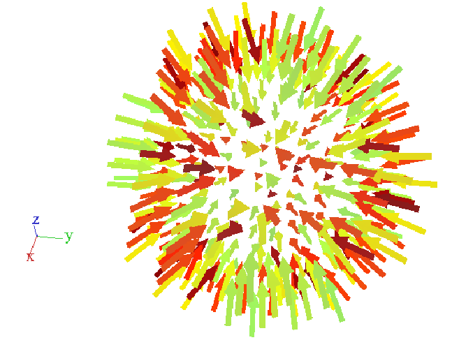
We then reformulate the dot-product in (6.3) as component-wise convolution of ${\bf\cal T}[r,\alpha]$ with ${\cal S}[r]({\bf x})$ :

T[r,\alpha]({\bf x}):=\sum\limits_{c=0}^{2}{\bf X}[c]\big|_{{\cal S}[r]({\bf x})}*{\bf\cal T}[r,\alpha][c],

(6.4)

where ${\bf X}({\bf x})[c]$ returns the $c$ th directional component of ${\bf X}({\bf x})$ . Hence, we can apply a fast convolution to simultaneously evaluate (6.4) at all voxels ${\bf x}$ :

T[r,\alpha]({\bf X}):=\sum\limits_{c=0}^{2}FFT^{-1}\big(FFT({\bf X}[c])\cdot FFT({\bf\cal T}[r,\alpha][c])\big).

(6.5)

For discrete input data we have to handle the implementation of the spherical template $T[r,\alpha]$ with some care. To avoid sampling issues, we apply the same implementation strategies as in the case of the Spherical Harmonic base functions (see section 2.1 for details).

Multi-Channel Data:

$1v$ -Features cannot directly combine data from several channels into a single feature. In case of multi-channel data, we would have to compute features for each channel separately.

Complexity

Using the convolution approach, we end up with a complexity of $O(m\cdot m\log m)$ for an input volume of size $m$ .

Parallelization:

Since there is no easy way to parallelize the Fourier Transform, we do not further parallelize the computation of $1v$ -Features. But since $1v$ -Features can be computed so fast anyway, this is not a real drawback.

6.1.3 Discussion

The $1v$ -Feature provides a very fast and rotation invariant method for the extraction of local features from 3D vector fields. The nature of the kernel vectors given as normals of the spherical neighborhood makes the $1v$ kernel an optimal detector for spherical structures which relies mostly on shape and hardly on texture properties of the underlying data. The $\alpha$ factor then indicates if we detect the inner or the outer surface of a spherical shape.
In an alternative interpretation, the $1v$ approach could be seen as Hough-Transform [18] for spheres. This could be reinforced by an additional integration over several radii.

6.2 2-Vector Features ( $2v$ )

The $2v$ -Feature uses a variation of the $1v$ kernel: instead of using the normal vectors of a spherical neighborhood template, the $2v$ kernel integrates over the similarities of the data vectors of the centering vector ${\bf X}({\bf x})$ .

6.2.1 Feature Design

Given a 3D vector field ${\bf X}:\mathbb{R}^{3}\rightarrow\mathbb{R}^{3}$ , we extract local features from the spherical neighborhoods ${\cal S}[r]({\bf x})$ at positions ${\bf x}$ .
The basic idea of the $2v$ kernel is to compute the similarity (in terms of the dot-product) of the direction of the data vectors ${\bf X}({\bf x}_{i}),\forall{\bf x}_{i}\in{\cal S}[r]({\bf x})$ with the direction of the center vector ${\bf X}({\bf x})$ .

Rotation Invariance:

If we plug the $2v$ kernel into the general Haar framework (4.2), we can achieve invariance regarding rotations ${\cal R(\phi,\theta,\psi)}\in{\cal SO}(3)$ which are parameterized in Euler angles (see section 1.2).
Just as in the $1v$ case, we use the fact that all possible positions of the ${\bf x}_{i}$ lie on the spherical neighborhood ${\cal S}[r]({\bf x})$ with the radius:

r=\big|{\bf x}-{\bf x}_{i}\big|,

(6.6)

And again, since we are considering only a singe kernel vector, we can reduce the integral over all rotations to an integral over all points of the spherical neighborhood parameterized by the angles $\phi$ and $\theta$ (see 4.9 for a detailed justification). The final formulation of the $2v$ -Feature is then:

T[r]({\bf x}):=\int\limits_{x_{i}\in{\cal S}[r]({\bf x})}\big\langle{\bf X}({\bf x}),{\bf X}({\bf x}_{i})\big\rangle\sin\theta d\phi d\theta.

(6.7)

6.2.2 Implementation

The implementation strictly follows the convolution based algorithm introduced for the $1v$ case (see section 6.1.2). The only difference is that the vectors in the template $\cal T$ are oriented in the same direction as $\bf X(x)$ .

Multi-Channel Data:

$v2$ -Features can combine data from two channels into a single feature: we can simply extract the kernel direction ${\bf X}[c_{1}]({\bf x})$ and the neighborhood data ${\bf X}[c_{2}]({\bf x}_{i})$ from different channels.

Complexity

Using the convolution approach, we end up with a complexity of $O(m\cdot m\log m)$ for an input volume of size $m$ .

Parallelization:

Since there is no easy way to parallelize the Fourier Transformation, we do not further parallelize the computation of $2v$ -Features. But as $2v$ -Features can be computed so fast anyway, this is not a real drawback.

6.2.3 Discussion

The fast $2v$ kernels return more texture based and less shape based features. Intuitively, $2v$ -Features are an indicator for the local homogeneity of the vector field. The name $2v$ -Feature might miss leading to some degree, since we only consider a single kernel vector. But in contrast to the $1v$ -Feature approach, we actually combine two vectors from the input data ${\bf X}({\bf x})$ and ${\bf X}({\bf x}_{i})$ .

6.3 n-Vector Features ( $nv$ )

The $nv$ -Features are the direct extension of the $np$ -Features (see section 4.3) to 3D vector fields. Analogous to the properties of $np$ kernels on scalar (multi-channel) data, the goal is to derive highly specific local features for the detection of local structures (objects) in 3D vector fields.
To obtain a strong discrimination power, we introduce a vectorial kernel which is able to handle an arbitrary number of kernel vectors ${\bf v}_{1},\dots,{\bf v}_{n}$ instead of only one or two (as for $1v,2v$ -Features).
Since the entire derivation of the $nv$ kernel strongly relies on the very same methods and algorithms that were introduced for the derivation of the $np$ kernel, the reader may to refer to section 4.3 for some technical details.

Given a 3D vector field ${\bf X}:\{\mathbb{R}^{3}\rightarrow\mathbb{R}^{3}\}$ , we extract local features from the spherical neighborhoods ${\cal S}[r]({\bf x})$ at positions ${\bf x}$ . For the kernel vectors ${\bf v}_{i}\in\{\mathbb{R}^{3}\times\mathbb{R}^{3}\}$ , we write $\dot{\bf v}_{i}\in\mathbb{R}^{3}$ and $\overrightarrow{{\bf v}_{i}}\in\mathbb{R}^{3}$ to address their position and direction.

There are two major differences in the basic formulation between general sparse and local scalar ( $np$ ) and vectorial $(nv)$ kernels: first, we do not explicitly consider a center vector for $nv$ kernels (even though the framework would allow such a constellation). The main reason to do so is given by the second difference: since non-linear mappings (like the $\kappa_{i}$ in the $np$ kernel) are not well defined on vectorial data, we do not use a separable kernel approach (4.5) for the construction of the $nv$ kernel.
Instead, we are following the alternative (fast) approach (4.31), which allows us to formalize the $n$ -Vector kernels in a more abstract way: (4.5):

\displaystyle\kappa\left(s_{g}({\bf v}_{1}),\dots,s_{g}({\bf v}_{n})\right).

(6.8)

Figure 6.4 shows an example $nv$ kernel. Later on, we give the actual kernel mapping $\kappa$ , which is still non-linear, but does not operate directly on vectorial data.

6.3.1 Feature Design

The primary goal is to achieve rotation invariance. Hence, the transformation group ${\cal G}$ is given by the group of 3D rotations ${\cal SO}(3)$ . If we parameterize these global rotations ${\cal R}\in{\cal SO}(3)$ as local rotations of the kernel vectors in Euler angles $s_{g}(\phi,\theta,\psi)$ (see Fig. 1.4), we can rewrite (6.8) as:

\displaystyle T[\Lambda]({\bf x})

\displaystyle:=

\displaystyle\int\limits_{{\cal SO}(3)}\kappa\left({s_{g}}_{(\phi,\theta,\psi)}({\bf v}_{1}),\dots,{s_{g}}_{(\phi,\theta,\psi)}({\bf v}_{n})\right)\sin{\theta}d\phi d\theta d\psi,

(6.9)

where $\Lambda$ is the set of parameters, i.e. including $\kappa$ - we define $\Lambda$ in detail when we present the parameterization of the kernel in the next sub-section(6.3.1).

Parameterization

The key for a fast computational evaluation of (6.9) is the smart parameterization of the kernel. Following the approach for the $np$ kernels, we parameterize the position of the kernel vectors as points $\dot{\bf v}_{i}$ with $i\in\{1,\dots,n\}$ located at concentric spherical neighborhoods ${\cal S}[r_{i}]\left({\bf x}\right)$ with radii $r_{i}$ surrounding the point of the feature extraction ${\bf x}$ . Hence, each $\dot{\bf v}_{i}$ is parameterized by the spherical angles $\Phi_{i}\in[0,\dots,2\pi],\Theta_{i}\in[0,\dots,\pi]$ and $r_{i}\in\mathbb{R}$ (also see figure 4.10).
The overall parameter set $\Lambda$ thus includes the parameterized position $\dot{\bf v}_{i}$ , the direction $\overrightarrow{{\bf v}_{i}}$ (which is normalized to $|\overrightarrow{{\bf v}_{i}}|=1$ ) and the non-linear mapping $\kappa$ which will be split into $\kappa_{1},\dots,\kappa_{n}$ later on:

\Lambda:=\big\{\{\kappa_{1},r_{1},\Phi_{1},\Theta_{1},\overrightarrow{{\bf v}_{1}}\},\dots,\{\kappa_{n},r_{n},\Phi_{n},\Theta_{n},\overrightarrow{{\bf v}_{n}}\}\big\}.

(6.10)

Given this parameterization, we further follow the approach from the $np$ derivation and introduce “delta like” vectorial template functions ${\cal T}_{i}$ which represent the kernel vectors ${\bf\cal T}_{i}[r_{i}]$ in the harmonic domain:

\big(\widehat{\bf\cal T}_{i}[r_{i},\Phi_{i},\Theta_{i},\overrightarrow{{\bf v}_{i}}]\big)_{km}^{l}=\overrightarrow{{\bf v}_{i}}^{T}{\bf Z}^{l}_{km}(\Phi,\Theta).

(6.11)

Now we have a frequency representation of the individual kernel vectors. In the next step, we evaluate the contribution of the input data at these kernels. For each feature evaluation, we perform Vectorial Harmonic expansions around ${\bf x}$ at the radii $r_{i}$ (associated with the position of the respective kernel vectors) of the input vector field $X$ :

\widehat{{\cal S}[r_{i}]}({\bf x})={\cal VH}[r_{i}]({\bf x}).

(6.12)

With the data and the kernel vectors represented in the harmonic domain, we can apply a fast correlation to evaluate the contribution of each kernel point on the local data and perform this evaluation over all rotations. Given a vector at position ${\bf x}$ , we compute the result $C^{\#}_{i}$ of this fast correlation over all spherical angles for the i-th kernel vector as shown in (1.80):

C^{\#}_{i}=\widehat{{\cal S}[r_{i}]}({\bf x})\#\widehat{\cal T}_{i}.

(6.13)

Rotation Invariance

As in the case of $n$ -Point kernels, we need to couple the contributions of the individual kernel vectors in such a way that only the chosen kernel constellation (given by the $\Phi_{i},\Theta_{i},r_{i}$ ) has a contribution to the feature while rotating over all possible angles, i.e. the positions of the kernel vectors must not rotate independently. Note that the correct orientation of the kernel vectors under the rotation is guaranteed by the Vectorial Harmonic formulation.
Since the $C^{\#}_{i}$ hold the contribution at each possible angle in a 3D Euclidean space with a ( $\phi,\theta,\psi$ ) coordinate-system (see section 1.8), we can perform the multiplicative coupling of the separate sub-kernels (4.5) by a angle-wise multiplication of the point-wise correlation results: $\prod_{i=2}^{n}C^{\#}_{i}$ .

By integrating over the resulting Euclidean space of this coupling, we easily obtain rotation invariance as in (6.9):

\displaystyle\int\limits_{{\cal SO}(3)}\left(\prod\limits_{i=2}^{n}{\cal C}^{\#}_{i}\right)\sin{\theta}d\phi d\theta d\psi.

(6.14)

Finally, we still have to introduce the non-linear mapping into (6.14) to satisfy (6.8) . We follow the fast approach from (4.31), where we split $\kappa$ into $n$ non-linear mappings $\kappa_{1},\dots,\kappa_{2}$ which act directly on the correlation matrices. This leads to the final formulation of the $nv$ -Feature:

\displaystyle T[\Lambda]({\bf x})

\displaystyle:=

\displaystyle\int\limits_{{\cal SO}(3)}\left(\prod\limits_{i=1}^{n}\kappa_{i}\big({\cal C}^{\#}_{i}\big)\right)\sin{\theta}d\phi d\theta d\psi.

(6.15)

Figure 6.5 shows a schematic overview of the computation of $nv$ -Features.

6.3.2 Implementation

The transformation into the harmonic domain is implemented as described in section 2.2. Hence, we can also obtain the expansions at all points in $X$ at once using the convolution approach analogous to (2.3).
The implementation of the template ${\cal T}_{t}$ has to be handled with some care: to avoid sampling issues, we apply the same implementation strategies as in the case of the Spherical Harmonic base functions (see section 2.2 for details).
The computation of the correlation matrices ${\cal C}^{\#}$ follows the algorithm given in section 1.8. The size of the padding $p$ we need to apply strongly depends on the angular resolution necessary to resolve the given configuration of the kernel points.
Finally, the evaluation of the Haar-Integration over all possible rotations is approximated by the sum over the combined $(\phi,\theta,\psi)$ -space:

\displaystyle T[\Lambda]({\bf x})

\displaystyle\approx

\displaystyle\sum\left(\prod\limits_{i=2}^{n}{\cal C}^{\#}_{i}\right).

(6.16)

Multi-Channel Data:

$nv$ -Features cannot directly combine data from several channels into a single feature. In case of multi-channel data, we have to compute features for each channel separately.

Complexity

The computational complexity of the $nv$ -Feature is dominated by the Vectorial Harmonic expansions needed to transform the input data and the kernel vector templates into the harmonic domain. This takes $O(b_{\max}\cdot m\log m)$ for input data of size $m$ and $O(n\cdot b_{\max}\cdot m^{\prime}\log m^{\prime})$ for a template size of $m^{\prime}$ . The costs for the correlation and multiplication of the correlation matrices are negligible.

Parallelization:

As stated in section 2.1, we can gain linear speed-up in the number of cores for the parallelization of the harmonic transformation. Further, we could also split the computation of the correlation matrices into several threads, but as mentioned before, this speed-up hardly falls into account.

6.3.3 Discussion

The $nv$ -Features provide a powerful framework for the implementation of local features which are able obtain invariance towards rotation via Haar-Integration.
In practice, $nv$ -Features are especially suitable for the design of highly specific features with a strong discriminative power used in challenging image analysis tasks justifying the higher computational costs. For less complex problems, we are better off using some of the less complex feature methods.

A major problem concerning the application of $nv$ -Features is the huge set of kernel parameters $\Lambda$ (6.10) we have to choose. In practice, it is infeasible to try all possible parameter combinations in a feature selection process, as we suggest for other features. Neither is it practically possible to select the best parameter settings by hand.

Chapter 7 Experiments

In the final chapter of the first part, we evaluate the feature methods which were introduced in the previous chapters. We start with the evaluation of the speed and accuracy of our fast correlation in Spherical Harmonics in section 7.1 and the correlation in Vectorial Harmonics in section7.3.
Section 7.2 evaluates the computational complexity of our features on real world data. Then we use a database of semi-artificial 3D textures (see Appendix A) to perform a series of 3D texture classification (see section 7.4).

7.1 Evaluating ${\cal SH}$ -Correlation

Unlike previous publications [26][27][25], which only performed a small set of experiments with a fixed number of predefined example rotations, we evaluate our methods with a series of large scale experiments on real word data.
If not mentioned otherwise, all experiments have the same basic setup: for each parameter set, we evaluate the error statistics of 100 random rotations of random objects. We generate the rotations over all possible angles $\phi,\psi\in[0,2\pi[$ and $\theta\in[0,\pi[$ with a resolution of $0.001\approx 0.1^{\circ}$ . Note that an error of $1^{\circ}\approx 0.017$ . All given error rates are the sums over the errors of all three angles.

Rotating Objects in the Harmonic Domain

In this first series of experiments, we extract a harmonic expansion with a fixed radius around the object center and then rotate this expansion using (1.19).

Pad Size:

In a first experiment, we are able to show the effect of our padding method on the estimation accuracy. Figure (7.1) clearly shows the correlation of the pad size and the expected error. It is also evident that we are able to achieve a high precision with errors below 1 degree. Hence, the experimental errors are found to be well within the theoretical bounds given in (1.52).

Maximum Band:

The next two experiments investigate the practical influence of the maximum expansion band on the estimation errors.

Figure (7.2) strongly supports our initial assumption that the original formulation is not able to achieve accurate estimates for low expansions. Our method on the other hand achieves very low error rates even for extremely low expansions with $b=2$ .

Rotational Invariance and Computational Costs:

Rotational Invariance and Computational Costs are investigated in the last two experiments (figure (7.3)) of the first series. We rotate the object in $\pi/8$ steps in every angle to show that the correlation maximum is stable and indeed independent of the rotation. The computational complexity is largely dominated by the costs for the inverse FFT, hence growing with the pad size. So accuracy comes at some cost but reasonable accuracy can still be achieved well within 1 second.

Rotating Objects in $\mathbb{R}^{3}$

The results of figure (7.2) suggest that the maximum expansion band has no influence on the quality of the rotation estimation - of course, this is only true if we are considering input signals that are limited to the very same maximum band. This is very unlikely for very low bands in the case of real data.
In order to evaluate the actual influence of the maximum expansion band, we need to rotate the objects in $\mathbb{R}^{3}$ and extract a second harmonic expansion after the rotation. As mentioned before, the usability of our sinc interpolation approach is limited to correctly sampled (concerning the Sampling Theorem) input signals (also see section 2 for more details on sampling issues). Hence, one must not expect to obtain precise rotation estimates for low band expansions, which act as a low pass filter, of high frequent input signals. Luckily, for most input data, we are not depending on the high frequent components in order to find the maximum correlation. Hence, we can apply a low pass filter (Gaussian) on the input data prior to the harmonic expansion.

Figure (7.4) shows the impact of the maximum band and smoothing for rotations in $\mathbb{R}^{3}$ . Overall, the estimation results are slightly worse than before, but are still quite reasonable.

7.2 Evaluating the Feature Complexity

We evaluated the computational complexity on dummy volume data. All experiments were conducted on a 3GHz machine with 16 CPU cores and 128GB Ram. However, only a single CPU was used if not noted otherwise.

7.2.1 Complexity of the Spherical Harmonic Transformation

We conducted two experiments to show the complexity of the voxel-wise Spherical Harmonic transformation of 3D volume data. The complexity is independent of the actual data and is only influenced by the maximum expansion band ( $b_{max}$ ) and the data size as shown in figure 7.5.

7.3 Evaluating ${\cal VH}$ -Correlation

We use a sample 3D vector field (see figure 7.6) which is rotated around the center of one spherical patch parameterized by a single radius of $r=10$ .

For each experiment, we evaluate the error statistics of 100 random rotations of this vector field. We generate the rotations over all possible angles $\varphi,\psi\in[0,2\pi[$ and $\theta\in[0,\pi[$ with a resolution of $0.001\approx 0.1^{\circ}$ . Note that an error of $1^{\circ}\approx 0.017$ . All given error rates are the accumulated errors of all three angles.

Figure 7.7 shows the direct effect of the maximum expansion band $b_{max}$ on the rotation estimate. But even for expensive “higher band” expansions, we encounter strong outliers and a rather poor average accuracy.
This can be compensated by our Sinc interpolation approach (1.49): Figure 7.7 shows how we can reduce the rotation estimation error well below $1^{\circ}$ , just by increasing the pad size $p$ . The additional computational costs caused by the padding are also given in figure 7.7.

Summarizing these first experiments, we are able to show that our proposed method is able to provide a fast and accurate rotation estimation even for rather low band expansions, e.g. if we choose $p=64$ and $b_{max}=5$ , we can expect an average estimation error below $1^{\circ}$ at a computation time of less than $25$ ms.

Key Point Detection.

In a second series of experiments, we evaluate the performance of our methods in a key point (or object) detection problem on artificial data. Figure 7.8 shows the 3D vector fields of two of our target structures. Our goal is to detect the center of such $X$ - and $Y$ -like shaped bifurcations under arbitrary rotations in larger vector fields. For each target structure, we extract a single patch, parameterized in four different radii with $b_{max}=3$ , at the center of the bifurcations.
Using (2.6), we extract patches with the same parameterization at each point of the test samples and apply our fast, combined (see section 1.4.6) and normalized (1.57 ) cross-correlation to detect the target structures in the test vector fields. Figures 7.9 and 7.10 show some example test data together with the correlation results.

It should be noted that the test bifurcations are only similar in terms of a $X$ or $Y$ shape, but not identical to the given target structures. We also rotate the test data in a randomized procedure over all angles.

Applying a threshold of $0.9$ to the correlation results, we were able to detect the correct target structures in all of our test samples without false positives.

7.3.1 Complexity of the Vectorial Harmonic Transformation

We also performed the experiment measuring the complexity in dependency of the maximum expansion band ( $b_{max}$ ) for the voxel-wise Vectorial Harmonic transformation of 3D volume data. Figure 7.11 clearly shows that the complexity of the transformation in the vectorial case is much higher than in the scalar case. This can only be compensated by the parallelization of the transformation.

7.3.2 Complexity of a voxel-wise Feature Extraction

In the final experiment regarding the computational complexity, we evaluated all features on a $(250\times 250\times 250)$ volume texture sample. We extracted voxel-wise features simultaneously at all voxels. We used a fixed radius of $r=10$ and evaluated the computation time on a single core with $b_{max}=\{3,5,8\}$ .

Figure 7.12 illustrates the computation time for all features which is also given in table 7.1. The complexity of the individual features has a wide range: from about 3 seconds for the computation of the simple $2p$ -Feature (which is not based on a Spherical Harmonic transformation), to almost 4 hours needed to compute a $4v$ -Feature with $b_{max}=8$ at every voxel of the $(250\times 250\times 250)$ volume.

It is obvious that some of the features are too complex to be of practical use in such a setting as presented here. Especially, a computation of the highly specialized $np$ and $vp$ -Features at all voxels and at a high expansion band $b_{max}$ appears to be practically intractable.
However, it turns out that this is not a major drawback in practice: First of all, as figure 7.13 shows, the features are well suited for parallelization, and second, it is usually not necessary to compute such specific features at all $256^{3}$ voxels. Typically, it is very easy to reduce the number of candidate voxels drastically, if one uses the response of “cheap” features to perform a rough pre-segmentation.

feature	$b_{max}=3$	$b_{max}=5$	$b_{max}=8$
${\cal SH}_{abs}$	46	102	229
${\cal SH}_{phase}$	190	848	4431
${\cal SH}_{autocorr}$	90	201	441
${\cal SH}_{bispectrum}$	157	422	1596
LBP	87	175	365
$2p$	3	3	3
$3p$	50	114	257
$4p$ (4)	470	1290	5965
$4p$ (1)	156	416	1468
$5p$ (5)	604	1624	6358
$5p$ (1)	201	506	1589
${\cal SH}$	40	93	198
${\cal VH}_{abs}$	558	896	1359
${\cal VH}_{autocorr}$	719	1515	4655
$1v$	455	455	455
$2v$	455	455	455
$3v$	1146	3003	11671
$4v$	1283	3751	14905
${\cal VH}$	513	823	1105

Table 7.1: Computational complexity of the individual features as illustrated in figure 7.12. The complexity was measured on a

(250\times 250\times 250)

volume texture sample with

r=10

and

b_{max}=\{3,5,8\}

using only a single CPU core.

Multicore Speed-up:

We examined the potential speed-up of a parallelization of the feature computation at the example of the $5p$ (5) feature (see table 7.1). Using 8 instead of a single CPU core, the complexity drops from 6350s (almost 2 hours) to 1700s ( $\approx$ 30min). Figure 7.13 shows how the parallelization affects the different computation steps like the ${\cal SH}$ transformation, the correlation step or the non-linear transformations and multiplications.

7.4 Evaluating 3D Texture Discrimination

In a final experiment, we evaluated the texture discrimination performance of our proposed features. The experiments were conducted on our artificial 3D volume texture database (see appendix A for details on this database).

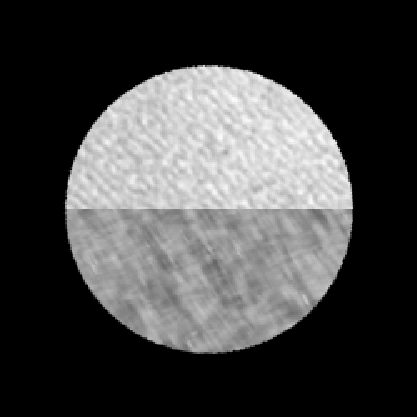
Using the SIMBA feature selection algorithm, we extracted the top 10 parameter combinations for each of our features. Scalar features were expanded to the 5th band, vectorial features were computed on the gradient field of the scalar input data and expanded to the 3rd band.
Given these feature vectors, we used a voxel-wise SVM classification to evaluate the 3D texture segmentation performance of the individual features.

feature	rotations	rotations and gray-scale changes
${\cal SH}_{abs}$	91%	82%
${\cal SH}_{phase}$	90%	90%
${\cal SH}_{autocorr}$	93%	94%
${\cal SH}_{bispectrum}$	94%	89%
LBP	91%	91%
$2p$	85%	78%
$3p$	86%	79%
$4p$ (4)	93%	93%
$4p$ (1)	92%	92%
$5p$ (5)	91%	91%
$5p$ (1)	91%	91%
${\cal VH}_{abs}$	94%	94%
${\cal VH}_{autocorr}$	95%	95%
$3v$	91%	91%
$4v$	93%	93%

Table 7.2: 3D texture segmentation benchmark. Voxel-vise error rate in percent.

4p

(4) indicates that the

4p

-Feature was computed with kernel points in 4 different channels(4.29 ), whereas

4p

(1) indicates the fast

np

-Feature version (4.31), where all kernel points are located in the same channel.

Our evaluation clearly shows that those features that are not invariant towards gray-scale changes strongly suffer in the case of such changes. The vectorial features appear to be very stable, however this comes at the cost of higher computational complexity (see table 7.1).
The highly specific $np$ and $vp$ -Features are not able to outperform the other approaches. These features are probably too selective to be able to describe the large variations in the textures by just 10 parameter settings. However, these features anyway have been designed for key point and object detections (see section 7.3) rather than texture description.

Appendix A Artificial 3D Volume Texture Database

The following tables show a few sample images of xy-slices taken from the training samples of our artificial 3D volume texture database.

A.0.1 Texture Generation

The volume textures were generated from 2D texture samples which were taken from the BFT texture data base provided by the University of Bonn (http://btf.cs.uni-bonn.de/download.html). Figure A.1 gives an overview of our very simple volume texture generation process.

The number of linear combinations $n$ , as well as the rotations ${\cal R}_{i}$ and factors $\alpha_{i}\in[0,1]$ are chosen randomly.

A.0.2 Base Textures

The database contains 10 “base samples” for each of the six different textures (texture 1-6), all of which have a normalized average gray-value. These “base samples” are used to generate separate training and test sets using arbitrary rotations and additive gray-value changes.

A.0.3 Texture Segmentation

Given the “base samples” of the 3D volume textures, we generated a simple texture segmentation benchmark. One half of the “base samples” was used to build $60$ labeled training samples (see figure A.3) and the other half was used for the test samples.
The $200$ test samples consist of random combinations of two textures with a ground-truth labeling, where each the textures was rotated randomly and subject to an additive gray-value change (see figure A.2).

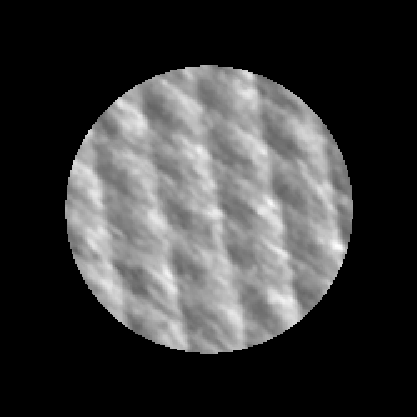
References

[1] R. Barrera, G. Estevez, and J. Giraldo. Vector spherical harmonics and their application to magnetostatic. Eur. J. Phys., 6:287–294, 1985.
[2] D. Brink and G. Satchler. Angular Momentum, Second Edition. Clarendon Press, Oxford, 1968.
[3] G. Burel and H. Henoco. Determination of the orientation of 3d objects using spherical harmonics. Graph. Models Image Process., 57(5):400–408, 1995.
[4] H. Burkhardt. Transformationen zur Lage Invarianten Merkmalsgewinnung. VDI-Fortschritt-Bericht, Reihe 10 (Angewandte Informatik), Nr. 7, VDI-Verlag Düsseldorf, 1979.
[5] H. Burkhardt and S. Siggelkow. Invariant features in pattern recognition - fundamentals and applications. In Kotropoulos, C., Pitas, I., editors, Nonlinear Model-Based Image/Video Processing ans Analysis, pages 269–3007, 2001.
[6] N. Canterakis. 3d zernike moments and zernike affine invariants for 3d image analysis and recognition. In 11th Scandinavian Conf. on Image Analysis, 1999.
[7] R. A. Crowther. The molecular replacement method. In M. Rossmann, editor, Gordon and Breach, New York, pages 173–178, 1972.
[8] H. Cundy and A. Rollett. Mathematical Models. Oxford Univ. Press, 2nd ed., 1961.
[9] P. K. D. Healy Jr., D. Rockmore and S. Moore. Ffts for the 2-sphere - improvements and variations. The Journal of Fourier Analysis and Applications, 9(4):341–385, 2003.
[10] J. Fehr and H. Burkhardt. Phase based 3d texture features. In Proceedings of the DAGM 2006, Springer LNCS 4174, pp 263-272, 2006.
[11] J. Fehr, M. Reisert, and H. Burkhardt. Fast and accurate rotation estimation on the 2-sphere without correspondences. In Proceedings of the ECCV 2008, LNCS 5303, pages 239–253, 2008.
[12] J. Fehr, O. Ronneberger, H. Kurz, and H. Burkhardt. Self-learning segmentation and classification of cell-nuclei in 3d volumetric data using voxel-wise gray scale invariants. Proceedings of the 27th DAGM Symposium, in number 3663 LNCS, Springer, Vienna, Austria, 30.8 - 2.9. 2005., 2005.
[13] J. Fehr, O. Ronneberger, J. Schulz, T. Schmidt, M. Reisert, and H. Burkhardt. Invariance via group-integration: A feature framework for 3d biomedical image analysis. In proceeding of the special session on Invariance And Robustness at the International Conference on Computer Graphics and Imaging (CGIM 2008), Innsbruck, Austria, 2008.
[14] M. Frigo and S. G. Johnson. The design and implementation of FFTW3. Proceedings of the IEEE, 93(2):216–231, 2005. special issue on ”Program Generation, Optimization, and Platform Adaptation”.
[15] H. Groemer. Geometric Applications of Fourier Series and Spherical Harmonics. Cambridge University Press, 1996.
[16] D. Healy, D. Rockmore, P. Kostelec, and S. Moore. Ffts for the 2-sphere - improvements and variations. Journal of Fourier Analysis and Applications, 9:4:341–385, 2003.
[17] E. Hill. The theory of vector spherical harmonics. Am. J. Phys., 22:211–214, 1954.
[18] P. Hough. Method and means for recognising complex patterns. Technical report, U.S. Patent No. 3069654, 1962.
[19] Y. Kangl, K. Morooka1, and H. Nagahashi. Scale invariant texture analysis using multi-scale local autocorrelation features. In Scale Space and PDE Methods in Computer Vision, LNCS 3459, 2005.
[20] M. Kazhdan. Rotation invariant spherical harmonic representation of 3d shape descriptors. Symp. on Geom. Process., 2003.
[21] R. Kondor. A complete set of rotationally and translationally invariant features for images. CoRR, abs/cs/0701127, 2007.
[22] J. A. Kovacs and W. Wriggers. Fast rotational matching. Acta Crystallogr, (58):1282–1286, 2002.
[23] R. Lenz. Group theoretical methods in Image Processing. Springer Verlag, Lecture Notes, 1990.
[24] A. Lohmann, D. Mendlovic, and G. Shabtay. Significance of phase and amplitude in the fourier domain. J. Opt. Soc. Am., 14:2901–2904, 1997.
[25] A. Makadia and K. Daniilidis. Direct 3d-rotation estimation from spherical images via a generalized shift theorem. In IEEE Conference on Computer Vision and Pattern Recognition, Madison, 2003.
[26] A. Makadia and K. Daniilidis. Rotation recovery from spherical images without correspondences. IEEE Transactions on Pattern Analysis and Machine Intelligence, 28(7), 2006.
[27] A. Makadia, L. Sorgi, and K. Daniilidis. Rotation estimation from spherical images. In International Conference on Pattern Recognition, Cambridge, 2004.
[28] M. Novotni. 3d zernike descriptors for content based shape retrieval. In In The 8th ACM Symposium on Solid Modeling and Applications, pages 216–225. ACM Press, 2003.
[29] H. Nyquist. Certain topics in telegraph transmission theory. Trans. AIEE, 47:617–644, 1928.
[30] M. Reisert. Efficient tensor voting with 3d tensorial harmonics. In Albert-Ludwigs-University Freiburg, Internal Report 2, February 2008, 2008.
[31] M. Reisert and H. Burkhardt. Irreducible group representation for 3d shape description. In Proceedings of the 28th Pattern Recognition Symposium of the German Association for Pattern Recognition (DAGM 2006), Berlin, Germany, pages 132–142. LNCS, Springer, 2006.
[32] M. Reisert and H. Burkhardt. Efficient tensor voting with 3d tensorial harmonics. In CVPR Workshop on Tensors, 2008, Anchorage, Alaska, 2008.
[33] O. Ronneberger. 3D Invariants for Automated Pollen Recognition. Dissertation, University of Freiburg, 2008.
[34] O. Ronneberger, H. Burkhardt, and E. Schultz. General-purpose object recognition in 3d volume data sets using gray-scale invariants - classifacation of airborne pollen-grains recorded with a confocal laser scanning microscope. In Proceedings of the 16th International Conference on Pattern Recognition, Quebec, Canada, 2002.
[35] O. Ronneberger and J. Fehr. Voxel-wise gray scale invariants for simultaneous segmentation and classification. In Proceedings of the 27th DAGM Symposium, in number 3663 LNCS, Springer, Vienna, Austria,, 2005.
[36] O. Ronneberger, J. Fehr, and H. Burkhardt. Voxel-wise gray scale invariants for simultaneous segmentation and classification – theory and application to cell-nuclei in 3d volumetric data. Internal report 2/05, IIF-LMB, University Freiburg, april 2005.
[37] M. Rose. Elementary Theory of Angular Momentum. Dover Publications, 1957.
[38] D. Saupe and D. V. Vranic. 3d model retrieval with spherical harmonics and moments. In Proceedings of the 23rd DAGM-Symposium on Pattern Recognition, pages 392–397, London, UK, 2001. Springer-Verlag.
[39] M. Schael. Invariant 3D Features. Technical Report 4/97, Albert-Ludwigs-Universität, Freiburg, Institut für Informatik, 1997.
[40] M. Schael and S. Siggelkow. Invariant grey-scale features for 3d sensor-data. In Proceedings of the International Conference on Pattern Recognition, volume 2, Barcelona, Spain, pages 531–535, 2000.
[41] P. Schröder and W. Sweldens. Spherical wavelets: efficiently representing functions on the sphere. In SIGGRAPH ’95: Proceedings of the 22nd annual conference on Computer graphics and interactive techniques, pages 161–172, New York, NY, USA, 1995. ACM.
[42] P. Schröder and W. Sweldens. Spherical wavelets: Texture processing. In P. Hanrahan and W. Purgathofer, editors, Rendering Techniques ’95. Springer Verlag, Wien, New York, August 1995.
[43] J. Schulz, T. Schmidt, R. Ronneberger, H. Burkhardt, T. Pasternak, A. Dovzhenko, and K. Palme. Fast scalar and vectorial grayscale based invariant features for 3d cell nuclei localization and classification. In Proceedings of the 28th Pattern Recognition Symposium of the German Association for Pattern Recognition (DAGM 2006), Berlin, Germany, 2006.
[44] H. Schulz-Mirbach. Anwendung von Invarianzprinzipien zur Merkmalgewinnung in der Mustererkennung. PhD thesis, Technische Universität Hamburg-Harburg, 1995. Reihe 10, Nr. 372, VDI-Verlag.
[45] H. Schulz-Mirbach. Invariant features for grey scale images. In F. K. G. Sager, S. Posch, editor, 17. DAGM-Symposium Mustererkennung, pages 1–14, 1995.
[46] M. Tinkham. Group Theory and Quantum Mechanics. Dover Publications, 1992.
[47] S. Trapani and J. Navaza. Calculation of spherical harmonics and wigner d functions by fft. applications to fast rotational matching in molecular replacement and implementation into amore. Acta Crystallogr, 62:262–269, 2006.
[48] S. Wenndt and S. Shamsunder. Bispectrum features for robust speaker identification. Acoustics, Speech, and Signal Processing, IEEE International Conference on, 2:1095, 1997.
[49] L. Yaroslavsky. Boundary effect free and adaptive discrete signal sinc-interpolation algorithms for signal and image resampling. Appl. Opt., 42(20):4166–4175, 2003.

On Invariance, Equivariance, Correlation and Convolution of Spherical Harmonic Representations for Scalar and Vectorial Data.

Abstract

NOTE 1:

NOTE 2:

Introduction and Perquisites

Structure of of the report:

0.1 Mathematical Notation

0.2 General Feature Design

0.2.1 Feature Extraction

0.2.2 Invariance

Group Transformations

General Techniques For The Construction Of Invariant Features

0.2.3 Robustness

0.2.4 Equivariance

0.3 Local Features

0.3.1 Local Features on 3D Volume Data

Gray-Scale Data

Multi-Channel Data

0.3.2 Local Features on 3D Vector Fields

0.4 Related Work

Chapter 1 Mathematical Background

1.1 Spherical Harmonics

1.1.1 Associated Legendre Polynomials

Properties:

1.1.2 Deriving Spherical Harmonics

1.1.3 Useful Properties of Spherical Harmonics

Orthonormality:

Symmetry:

Addition Theorem:

1.2 Rotations in 𝒮ℋ{\cal SH}

1.2.1 Computation of Wigner d-Matrices

Recursive Computation of Wigner D-Matrices

1.2.2 Properties of Wigner Matrices

Orthogonality:

Symmetry:

Relations to Spherical Harmonics:

Relations to Legendre Polynomials:

1.3 Clebsch-Gordan Coefficients

1.3.1 Properties of Clebsch-Gordan Coefficients

Exceptions:

Orthogonality:

Symmetry:

1.4 Fast and Accurate Correlation in 𝒮ℋ{\cal SH}

Correlation on the 2-Sphere:

Rotation Estimation:

Related Approaches:

Rotation Estimation via Correlation:

1.4.1 Basic 𝒮ℋ{\cal SH}-Correlation Algorithm

1.4.2 Euler Ambiguities

1.4.3 Increasing the Angular Resolution

Sinc Interpolation.

Implementation:

1.4.4 Rotation Parameters

1.4.5 Normalized Cross-Correlation

1.4.6 Simultaneous Correlation of Signals on Concentric Spheres

1.4.7 Complexity

Parallelization:

1.5 Convolution in 𝒮ℋ{\cal SH}

1.5.1 “Left”-Convolution

1.5.2 Fast Convolution over all Angles

1.6 Vectorial Harmonics

1.6.1 Deriving Vectorial Harmonics

1.6.2 Useful Properties of Vectorial Harmonics

Orthonormality:

1.7 Rotations in Vectorial Harmonics

1.8 Fast Correlation in Vectorial Harmonics

1.9 Fast Convolution in Vectorial Harmonics

Chapter 2 Implementation

2.1 Discrete Spherical Harmonic Transform

2.1.1 Correct Sampling

2.1.2 Band Limitation bmaxb_{\max}

2.1.3 Invariance

Gray-Scale Robustness

Scale Normalization

Resolution Robustness

2.1.4 Complexity

2.1.5 Parallelization

2.1.6 Fast Spherical Harmonic Transform

2.2 Discrete Vectorial Harmonic Transform

2.2.1 Gray-Scale Invariance

On Invariance, Equivariance, Correlation and Convolution of Spherical Harmonic Representations
for Scalar and Vectorial Data.

1.2 Rotations in ${\cal SH}$

1.4 Fast and Accurate Correlation in ${\cal SH}$

1.4.1 Basic ${\cal SH}$ -Correlation Algorithm

1.5 Convolution in ${\cal SH}$

2.1.2 Band Limitation $b_{\max}$

Chapter 3 ${\cal SH}$ -Features

3.1 ${\cal SH}_{abs}$

${\cal SH}_{abs}$ Ambiguities:

3.2 ${\cal SH}_{phase}$

3.3 ${\cal SH}_{autocorr}$

3.4 ${\cal SH}_{bispectrum}$

4.1 2-Point Haar-Features ( $2p$ )

4.2 3-Point Haar-Features ( $3p$ )

4.3 $n$ -Point Haar-Features ( $np$ )

Chapter 5 ${\cal VH}$ -Features