Theoretical determination of Ising-type transition by using the Self-Consistent Harmonic Approximation
Abstract
Over the years, the Self-Consistent Harmonic Approximation (SCHA) has been successfully utilized to determine the transition temperature of many different magnetic models, particularly the Berezinskii-Thouless-Kosterlitz transition in two-dimensional ferromagnets. More recently, the SCHA has found application in describing ferromagnetic samples in spintronic experiments. In such a case, the SCHA has proven to be an efficient formalism for representing the coherent state in the ferromagnetic resonance state. One of the main advantages of using the SCHA is the quadratic Hamiltonian, which incorporates thermal spin fluctuations through renormalization parameters, keeping the description simple while providing excellent agreement with experimental data. In this article, we investigate the SCHA application in easy-axis magnetic models, a subject that has not been adequately explored to date. We obtain both semiclassical and quantum approaches of the SCHA for a general anisotropic magnetic model and employ them to determine various quantities such as the transition temperature, spin-wave energy spectrum, magnetization, and critical exponents. To verify the accuracy of the method, we compare the SCHA results with experimental and Monte Carlo simulation data for many distinct well-known magnetic materials.
Keywords:
Magnetism; Self-Consistent Harmonic Approximation; Ising-type transitionI Introduction and motivation
The continuous advancements in material science have driven the device miniaturization to sizes approaching the atomic scale. In this scale, dimensionality plays a crucial role and, usually, the three-dimensional Physics of macroscopic models does not apply as one might expect. An example of this is the Berezinskii-Thouless-Kosterlitz (BKT) transition, defined by a topological phase transition exclusively of two-dimensional models with order parameters exhibiting continuous symmetry, typically found in magnetic models with easy-plane anisotropy. The BKT transition was initially confirmed in the superfluid state of thin Helium filmsBishop and Reppy 1978, as well as in controlled experiments involving ultracold trapping of 2D Bose gasHadzibabic et al. 2006. Although the theoretical analysis of BKT transition has been performed in magnetic models over the years, obtaining experimental results has been challenging due to the difficulty of finding genuine two-dimensional magnetic materials with planar anisotropy. In many cases, the systems studied are quasi-two-dimensional magnets composed of weakly coupled layers. It is only recently that the synthesis of two-dimensional magnetic compounds, such as those based on rare-earth oxide YbMgGaO4Li et al. 2020a; Shen et al. 2019, has made it possible to observe the occurrence of the BKT transition in magnetic modelsLi et al. 2020b.
Contrary to the easy-plane scenario, we have the 2D magnetic models with easy-axis anisotropy, which break the continuous internal symmetry and provide an Ising-type transition. It should be noted that in this case, the Mermin-Wagner theorem does not apply, and even a minor anisotropy is sufficient to induce a finite transition temperature Bander and Mills 1988; Gouvêa et al. 1999; Cuccoli et al. 2000. In addition, since the first synthesis of graphene monolayersNovoselov et al. 2004, there has been tremendous interest in utilizing low-dimensional materials for technological applications. Specifically, numerous studies focused on the deployment of spintronic devices, which employ spin rather than electronic charge for processing and storing informationAhn 2020; Liu et al. 2020. However, graphene is a strongly diamagnetic material and shows a weak spin-orbit couplingAvsar et al. 2020, which hinders its effectiveness as a spin current detector via Inverse Spin-Hall EffectSaitoh et al. 2006. On the other hand, the recent development of the 2D van der Waals magnetsGong et al. 2017; Burch et al. 2018; Jiang et al. 2021 has further intensified research in low-dimensional magnets. For instance, Torelli et al. used Monte Carlo simulation models to investigate the role of anisotropy in several two-dimensional magnetsTorelli et al. 2019, some of which exhibit order even at room temperature.
As it is well-known, there is no theoretical method capable of yielding exact results in two-dimensional magnetic models, and approximations are required to extract any physical information about the system. Among the most traditional methods, we have bosonic representations such as the Holstein-Primakoff (HP), Schwinger, and Dyson-Maleev formalism, which replace the spin by magnon annihilation/creation operators (for a review of bosonic representations, and other methods, see Ref. Auerbach 2012; Pires 2021. Each method is more or less convenient depending on the magnetic system properties, but in the simpler description of non-interacting spin waves, they all result in quadratic models. However, eventually, the traditional quadratic representation is not suficient to describe the properties even as an initial approximation. In the spin conductivity evaluation, for example, the first non-null contributions arise from terms associated with interacting magnonsSentef et al. 2007. These contributions necessitate the inclusion of terms beyond the second order in the Hamiltonian. In these scenarios, an extensive perturbative analysis is required, and the solution can be hard to be obtained. Therefore, the SCHA formalism emerges as an alternative to the traditional bosonic representations in order to address these complexities.
The main idea of the SCHA is the replacement of the original spin Hamiltonian by another one containing only quadratic terms, similar to the aforementioned methods, involving the canonically conjugate fields (operators, in the quantum approach) and . However, unlike the Holstein-Primakoff formalism, the SCHA includes spin fluctuations through self-consistently solved renormalization parameters. Therefore, the SCHA model is simultaneously simple and precise in determining the thermodynamics of ordered phases in magnetic materials. Indeed, over the years, the SCHA has been successfully used to determine the critical temperature Pires et al. 1994; Pires 1995; Pereira et al. 1995; Costa et al. 1996; Pires 1997; Gouvêa et al. 1999, the topological BKT transition Menezes et al. 1992; Pires and Gouvea 1993; Pires et al. 1994; Pires 1994; Pires 1996a; Pires 1996b; Costa et al. 1996; Pires 1996c; Pires 1999; Pires and Gouvêa 2005; Gouvêa and Pires 2005; Pires et al. 2008a; Pires 2018, and the large-D quantum phase transition Pires 2007; Pires et al. 2008b; Pires and Gouvea 2009; Pires and Costa 2009; Moura et al. 2014 in a wide variety of magnetic models. In addition, the description by using canonically conjugate fields supply the most convenient formalism to describe coherent states in magnetism, as demonstrated by Moura and LopesMoura and Lopes 2019. More recently, Moura has applied the same formalism to present a detailed theoretical analysis of the ferromagnetic resonance and spin pumping process at the ferromagnetic/normal metal junctionMoura 2022.
In this paper, we employ the SCHA to analyze ferro and antiferromagnetic 2D models exhibiting easy-axis anisotropy. While the method has been extensively utilized to investigate magnetic models with easy-plane anisotropy, we have a dearth of studies focusing on the effects of easy-axis anisotropy. Therefore, we developed the SCHA formalism for determining the properties of anisotropic two-dimensional magnetic models, which are given by the Hamiltonian
| (1) |
where () represents the ferromagnetic (antiferromagnetic) coupling, is the (bare) anisotropic constant, and the first sum is carried out over nearest-neighbor sites. The last term is the Zeeman energy associated with the magnetic field . For a thin film, we can write , where is the external -field and is the demagnetizing field. Here, we are considering the special case with uniform magnetization along the x-axis that provides the demagnetization factors , while . In the antiferromagnetic case, , and there is no demagnetizing field to be considered. For ferromagnetic models, the demagnetizing field effects are considered replacing by an effective anisotropy, as demonstrated in the next section. To facilitate the application of the SCHA formalism, we consider sites located on the yz-plane while the anisotropy is defined along the x-axis. The easy-axis anisotropy is achieved by setting , and the limit approaching infinity corresponds to the Ising model. Alternatively, a uniaxial anisotropy, which also represents easy-axis anisotropic systems, could be considered in replacement of with minor modifications. Moreover, other interactions or anisotropies can be easily implemented, enabling the application of formalism in a wide variety of situations. The SCHA proves to be a valuable tool for determining essential properties of the ordered phase, such as the spectrum energy, the transition temperature, the magnetization, and others. The results obtained from SCHA exhibit excellent agreement with numerous experimental and Monte Carlo simulation studies.
II The SCHA formalism
As mentioned earlier, the initial step of the SCHA formalism is replacing the spin fields with quadratic representations of angle around the z-axis and its conjugate momentum, denoted as . Typically, in problems covering planar anisotropy, we consider spins located on the xy-plane and define the quantization along the z-axis. However, this choice is not mandatory. In the present context, to properly apply the SCHA formalism, we opt to place the spins on the yz-plane, while retaining the x-axis as the magnetization axis, as shown in Fig. (1).

Due to the anisotropy, and thus, the transverse spin components and are much smaller than the longitudinal component . From the classical point of view, the fields and , on sites i and j, respectively, satisfy the Poisson bracket , and the quantization is achieved by promoting the fields to operators that obey the commutation relation .
We can consider the spin as a quantum operator from the beginning, and then use the Villain representationVillain 1974 to represent the raising operator as , where . Alternatively, we can start in the semiclassical limit, for which the spins are represented by three-dimensional vectors. Then, we perform the quantization by the usual second quantization procedure. Since the second approach is more convenient for the present scenario, we will proceed with this approach.
Semiclassical approach
To begin with, we write the Hamiltonian (1) in terms of the and fields, which results in
| (2) | |||||
where , , and . In the above equation, for the antiferromagnetic model, we apply a rotation of around the z-axis for one of the sublattices. The quadratic Hamiltonian is then obtained by expanding the cosines and the function in terms of and . The dynamics of relies on the choice of Hamiltonian used to determine the time derivative, whether it is or . The resulting dynamics are strongly affected by whether the quadratic Hamiltonian or the complicated full version is used. To address this issue, we introduce renormalization parameters , , and replacing the cosine functions , , and with the terms , , and , respectively. The determination of the renormalization parameters aims to optimize the harmonic model, providing the most accurate representation of the system’s behavior. Therefore, the quadratic Hamiltonian, in momentum space, is expressed as
| (3) |
where , . The matrix coefficients are expressed as and . Here, , with . Note that, for antiferromagnetic models, and . The renormalization parameters are based on an alternative expansion of the angular part. By adopting the ansatz and , it is a straightforward procedure to demonstrate that the revised expansion yields the same Hamiltonian with
| (4a) | |||
| (4b) |
For the square lattice, the structure factor is written as , considering the unitary lattice parameter, and the number of nearest neighbors is . In Appendix A, we show that the renormalization parameters are obtained from two coupled self-consistent equations given by
| (5a) | |||||
| (5b) |
where we use the harmonic Hamiltonian for evaluating the averages. In the semiclassical limit, the Hamiltonian consists of two independent fields, and the thermodynamic averages can be easily determined. Extending the integration limit to , we deal with Gaussian integrals that provide
| (6) |
| (7) |
and
| (8) |
where we define the dimensionless reduced temperature . The integrals are carried out in the first Brillouin zone with the correspondent area denoted as .

Note that, for small anisotropies, , the deviation between the parameters , , and is negligible. Indeed, for small , we can write and . Fig. (2) shows the dependence on the temperature for the renormalization parameters , , , and , in an antiferromagnetic model with . For this case, the critical temperature provided by the self-consistent equations is . Using Eq. (11), demonstrated below, the critical temperature is given by .
The spin dynamics is obtained from the Hamilton equations and , which yield the coupled transverse spin equations
| (9a) | |||||
| (9b) |
By adopting the typical elliptical oscillating transverse behavior of the spin field, characterized by the solutions and , with representing the the transverse amplitudes, we obtain the spin-wave energy . At the low-temperature limit, the renormalization has a minor effect, and we can assume (at , it is easy to show that ). Therefore, the spin-wave energy takes on a simpler form denoted as for ferromagnetic insulator, and for antiferromagnetic one, where we define the temperature-dependent renormalized coupling . Note that represents the exchange coupling obtained from experiments at finite temperatures, while the bare value is the physical parameter only at zero temperature. In addition, due to the anisotropy, both cases show an energy gap, which vanishes when , that suppresses the spin fluctuations resulting in a finite transition temperature. In the long-wavelength limit, the ferromagnetic model shows the usual non-relativistic behavior with , where represents the deviation from the isotropic limit. Considering , the antiferromagnet also presents the non-relativistic energy in contrast to the relativistic spectrum obtained in the isotropic model.
At finite temperatures, the evaluation of the renormalization parameters entails the resolution of the system of coupled equations given by Eq. (5a). Generally, we perform this assessment through the utilization of self-consistently numeric integration techniques. Nevertheless, under the condition of small anisotropy (), we can acquire an analytical expression for . In this case, , even at high temperatures, close to . Therefore, we can simplify Eq. (7) for obtaining , where
| (10) |
The self-consistent equation exhibits an abrupt non-physical vanishing at the critical temperature . The same behavior is observed in the magnetization obtained from SCHA, as described subsequently. Consequently, this phenomenon leads to an erroneous first-order transition for magnetization. Such anomalies are frequently encountered in theories based on harmonic expansions. Nevertheless, despite this limitation, for temperatures , the SCHA method provides excellent results, while the formalism exhibits an issue only at temperatures very close to . It is worth noting that even for traditional spin representations, such as the Holstein-Primakoff formalism, it is difficult to properly describe the thermodynamics close to the critical temperature. Despite the excellent agreement in the low-temperature regime, when adopting the non-interacting spin-wave limit, the HP representation provides poor results for . In this scenario, it is necessary to incorporate the quartic-order terms, which renormalize the spin-wave energy and thereby furnish a more reasonable critical temperatureLow 1963. On the other hand, the critical temperature obtained from the harmonic approximation is very close to the real critical temperature. Therefore, notwithstanding the imprecise behavior at , we will consider as a reasonable estimation for the critical temperature. Using the condition , at the critical temperature, it is a straightforward procedure to reach the result
| (11) |
where is the base of the natural logarithm. In Sec. (III), we will apply Eq. (11) to determine the critical temperature of many experimental and Monte Carlo simulation studies.
Due to the easy-axis anisotropy, the spontaneous magnetization occurs in the direction perpendicular to the yz-plane and . Taking into account the uncoupled harmonic fields and , the average for the ferromagnetic model is simply expressed as
| (12) |
where we expand the square root up to first-order and use the equality , valid for Gaussian distributions. In the above equation, represents the saturation magnetization. For the antiferromagnetic model, it is necessary to analyze each sublattice separately, which results in
| (13) |
where the averages are reduced by two because the sublattice average takes into account only half of the sites.
Quantum approach
Although the semiclassical approach proves highly effective in solving large spin models, it is imperative to treat models featuring half-integer spin as purely quantum models. In the case of planar anisotropy, the quantum SCHA has been formulated by considering the spins in Hamiltonian either as operatorsVillain 1974; Pires 1997 or through the quantization of classical fieldsPires and Gouvea 1993. Regardless of which mode we used, the final results coincide. Hence, a resembling construction is expected for the easy-axis anisotropic model, and given our prior development of the classical SCHA, we proceed to quantize the Hamiltonian (3) following the conventional procedure of second quantization.
Within the quantum framework, the fields and are replaced by operators that satisfy the commutation relation . Consequently, it becomes advantageous to represent the Hamiltonian in terms of annihilation and creation operators. In favor of the bosonic operators and , we perform the transformation
| (14a) | |||||
| (14b) |
to yield the quantum harmonic Hamiltonian , where the magnon energy is (identical to the spin-wave energy obtained from the semiclassical analysis). The self-consistent equations are the same as given by Eq. (5a) except that is replaced by , and the averages must be determined by using the magnon number states (eigenvalues of ). Therefore, we obtain
| (15) |
and
| (16) |
Note that, in the semiclassical limit, , and the series expansion provides the same averages as those obtained in the previous section. However, due to the complexity of the average equations, it is not feasible to derive a quantum version of Eq. (11). Therefore, we can determine the critical temperature only by solving the quantum self-consistent equations. Furthermore, quantum fluctuations persist even at zero temperature, resulting in significant reductions in the renormalization parameters across the entire temperature range, as shown in Fig. (3).

III Applications of the SCHA
In this section, we employ the SCHA for describing a large number of studies involving easy-axis anisotropic models. In the description of two-dimensional ferromagnetic materials, certain experimental investigations have adopted a theory based on an external staggered magnetic field, which breaks the symmetry and provides ordering across all temperatures, as a means to describe the anisotropic behavior. However, following Cuccoli et. al.Cuccoli et al. 2000, we favor the utilization of the easy-axis anisotropy, as it aligns more closely with physical plausibility and yields satisfactory outcomes.
In the subsequent paragraphs, we utilize the SCHA to analyze some experimental data of antiferromagnetic systems. Among these systems, Rb2MnF4Birgeneau et al. 1970; Wijn et al. 1971; de Wijn et al. 1973; Cowley et al. 1977, Rb2MnCl4Schröder et al. 1980; Rauh et al. 1986, K2MnF4de Wijn et al. 1973; Birgeneau et al. 1973, and (CH3NH3)2MnCl4Schröder et al. 1980 exhibit a square crystalline lattice and possess large spin value of , which allow the effective application of the semiclassical approach. In addition, we include an model given by the K2NiF4]Skalyo et al. 1969; Birgeneau et al. 1971; de Wijn et al. 1973 compound. For the spin value, the semiclassical approach does not provide good results as occurs for the case, and a quantum analysis is necessary.
For a proper description, instead of using a pre-determined coupling constant and anisotropy, which are determined for other models rather than SCHA, we use the spectrum energy data to find the best parameters to fit the experimental measurement. For antiferromagnetic models, the gap is expressed as , which provides the anisotropy deviation . The renormalized coupling, at temperature , is then determined by applying the minimum square method to the error , where is the experimental energy data, measured at , and the momentum sum is done over the experimental values. The minimization in relation to yields
| (17) |
which is self-consistently solved to find . Finally, we solve Eq. (5a) at to determine the bare coupling constant , which is temperature independent and used to obtain the SCHA outcomes that are listed in Table (1). Since , the critical temperature is evaluated through the self-consistent equations and using Eq. (11). Details about each one of the compounds are listed below.
Rb2MnF4 - Based on Ref. Cowley et al. 1977, we obtain the gap energy meV (5.92 K), measured at K, which provides . The bare coupling constant calculated is given by K. The critical temperature obtained from SCHA is in remarkable agreement with the experimental data.
K2MnF4 - From the Ref. Birgeneau et al. 1973, we extract the energy gap meV (7.53 K) at K. The anisotropy is determined as , while the exchange constante is K. In this case, the evaluated critical temperature is also in good agreement with the real value.
Rb2MnCl4 - The data from Ref. Schröder et al. 1980, gives the energy gap K, determined at K. For , we find and K, which results in a critical temperature of approximately 9 percent larger than the experimental value.
MAMC - The organic chloride compound (CH3NH3)2MnCl4 (abbreviated MAMC) shows a structure similar to the Rb2MnCl4. Using the data of Ref. Schröder et al. 1980, measured at K, we obtain K and , using . In this case, the critical temperature obtained from SCHA is almost 10 percent larger than the real value.
K2NiF4 - This is the one analyzed compound with . Due to the small spin value, the semiclassical provides only a qualitative result, and better results are achieved through the quantum approach. From the Ref. (Birgeneau et al. 1971), we get the energy gap meV, measured at K, which results in K and in .
| Compound | Spin | Eq. (11) | SC-SCHA | Q-SCHA | Exp. |
|---|---|---|---|---|---|
| Rb2MnF4 | 5/2 | 39.0 K | 38.7 K | 36.4 K | 38.4 Ka |
| K2MnF4 | 5/2 | 44.1 K | 43.6 K | 41.0 K | 42.1 Kb |
| MAMC | 5/2 | 49.7 K | 49.5 K | 45.3 K | 45.3 Kc |
| 2.28 | 45.6 K | 45.4 K | 42.1 K | 45.3 K | |
| Rb2MnCl4 | 5/2 | 61.1 K | 60.2 K | 56.0 K | 56.0 Kc |
| 2.32 | 56.9 K | 56.1 K | 52.8 K | 56.0 K | |
| K2NiF4 | 1 | 85.7 K | 84.7 K | 98.1 K | 97.2 Kd |
a Phys. Rev. B 15, 4292 (1977)
b Phys. Rev. B 8, 304 (1973)
c Phys. Status Solidi (B) 97, 501 (1980)
d Phys. Rev. B 3, 1736 (1971)

Fig. (4) shows the energy spectrum for the four compounds listed in Table (1), taking into account a spin value of . The parameters and were adjusted to achieve the optimal fit between theoretical predictions and experimental data. The SCHA formalism yields a notable agreement, as observed.
The critical temperature for different compounds, namely Rb2MnF4, K2MnF4, Rb2MnCl4, and MAMC, was determined using the SCHA. The results indicate that is in notable agreement with experimental values for Rb2MnF4 and K2MnF4, while for Rb2MnCl4 and MAMC, the calculated is approximately 10 percent higher than the actual value. Generally, theoretical methods are better for describing Rb2MnF4 and K2MnF4. For instance, Pich and Schwabl applied the method of Callen to evaluate Green’s function for the same compounds listed in Table (1) and they also obtained better agreement for Rb2MnF4 and K2MnF4 rather than Rb2MnCl4 and MAMCPich and Schwabl 1994; Pich and Schwabl 1995. In their studies, the spin was replaced by an effective spin , accounting for quantum and thermal renormalizations. Cuccoli et. al. have applied the pure-quantum self-consistent harmonic approximation Cuccoli et al. 1992, a different harmonic approximation based on Weyl quantization for determining thermodynamic averages, to successfully estimate the critical temperature of Rb2MnF4Cuccoli et al. 2000. Conversely, Random Phase Approximation formalism have been used for Rb2MnCl4Radošević et al. 2009 and MAMCRadošević et al. 2011 to obtain more precise values for .
To improve the results for Rb2MnCl4 and MAMC, we also adopt an effective spin in place of , as explored in Ref. Pich and Schwabl 1994. Taking an interesting perspective, Köbler has considered the interaction between magnons and Glashow-Weinberg-Salam (GWS) bosons of the magnetic continuum field to explain the energy gap and the behavior in the long-wavelength limit of various magnetic modelsKöbler 2015. According to this approach, due to the magnon-GWS boson interaction, the spin of Rb2MnCl4 was reduced from to . Here, we used Eq. (11) to estimate the effective spin that results in a critical temperature close to the experimental values, obtaining for MAMC, and for Rb2MnCl4, close to the values of Ref.Pich and Schwabl 1994. Both critical temperature values, using and are listed in Table 1.

Fig. (5) shows the magnetization dependence on temperature for the four compounds. The outcomes derived from the SCHA exhibit a moderate level of concordance with experimental data. Specifically, when applied to the compound Rb2MnF4, the agreement between theoretical predictions and experimental observations is notably less pronounced. A potential remedy for this discrepancy is given by incorporating spin interactions that extend beyond the nearest-neighbors coupling. Cowley et al. adopted interactions between nearest and next-nearest neighbors to describe Rb2MnF4Cowley et al. 1977. This extended model yielded agreement with experimental results that was threefold superior to the conventional model, which solely considers nearest-neighbor coupling. It is noteworthy, however, that including these additional interactions within the SCHA formalism falls outside the scope of the present study. Considering the power-law behavior for the magnetization over the entire temperature interval, we obtain an almost uniform parameter, varying between (Rb2MnCl4) up to (K2NiF4). It is well-known, from the critical phenomena theory, that the power-law behavior is expected only close to the critical temperature, and the parameter must be determined around . Adopting the interval , we use the SCHA results for determining the critical exponent, and the obtained values are exhibited in Table (2). Provided the complicated behavior close to the critical temperature, it is not expectable a precise result for and so, the critical exponents show only a moderate agreement with experiments. The same problem is also obtained by using other theoretical formalisms, and a precise analysis at the critical point is not simple. In addition, note that close to , we have , and the magnetization exhibits a rapid decreasing that justifies the difficult to obtain measurements in the interval around to the critical temperature. For instance, the experimental values of are known for Rb2MnF4 ()Birgeneau et al. 1970, K2MnF4 ()de Wijn et al. 1973, MAMC ()Schröder et al. 1980, and K2NiF4 ()Birgeneau et al. 1970; Birgeneau et al. 1971.
| Rb2MnF4 | K2MnF4 | MAMC | Rb2MnCl4 | K2NiF4 | |
|---|---|---|---|---|---|
| SCHA | 0.155 | 0.132 | 0.165 | 0.121 | 0.187 |
| Exp. | 0.16 a | 0.15b | 0.18c | - | 0.138d |
a Phys. Rev. B 1, 2211 (1970)
b Phys. Rev. B 8, 304 (1973)
c Phys. Status Solidi (B) 97, 501 (1980)
d Phys. Rev. B 3, 1736 (1971)
The aforementioned results were obtained utilizing the semiclassical (SCHA) approach. However, an alternative quantum approach can also be employed to determine the critical temperature. In this case, the same procedure is followed to obtain the values of and , which exhibit slight differences when determined using the quantum SCHA approach. As expected, the spectrum energy presents excellent agreement with the experimental data. However, the calculated critical temperature exceeds the experimental value. To address this discrepancy, we adopt a correction method developed by Ariosa and Beck, which is specifically designed to determine the BKT transition using the SCHA approachAriosa and Beck 1992. The authors argue that topological excitations show excessive energy, leading to an elevated critical temperature. The issue arises due to the replacement of the periodic cosine function by , which displays a single bump at . In our particular case, there are no vortex solutions; however, the excessive energy resulting from magnon excitations persists. Indeed, consider the full probability function , where is a dimensionless parameter representing the reduced temperature, and the quadratic alternative ( and are normalization factors). Numeric integration for small values of reveals that . For example, when considering the interval , we find that and , when . However, for , the discrepancy increases, resulting in and . A similar observation can be made in the SCHA, where governs the average convergence. Observe that, in this case, we include the renormalization factor for considering the real magnon energy in the calculation. In the semiclassical limit, , the SCHA method offers a more accurate approximation compared to the quantum limit, where the renormalization parameter is smaller than the semiclassical limit resulting in a larger .
Therefore, following Ariosa and Beck, an improvement is achieved considering a three-bump probability function defined by , where denotes the probability function associated with a single bump at and represents the probability for to fall outside the interval . The angle average is then replaced by , where
| (18) |
and erf is the error function. Replacing the index by , we obtain a similar equation for . The critical temperatures obtained through the quantum SCHA, endowed with the above correction, are presented in Table (1). The obtained values of exhibit good agreement with experimental data. It is worth noting that, when utilizing the quantum approach, Rb2MnCl4 and MAMC demonstrate improved results when considering rather than the effective spin.
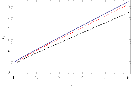
From an experimental standpoint, there is a limited availability of compounds with significant anisotropy. However, materials with large anisotropy can be studied by theoretical and computational simulation methods. Fig. (6) shows the results of SCHA, () RPA analysis, and classical Monte Carlo simulationTorelli and Olsen 2018 regarding the relationship between critical temperature and anisotropy. The outcomes of (semiclassical) SCHA and RPA methods display close agreement, while the MC data yields lower values of .
IV Summary and Conclusions
This paper explores the application of the Self-Consistent Harmonic Approximation (SCHA) to investigate two-dimensional magnetic models characterized by easy-axis anisotropy. While the SCHA formalism has been extensively employed to study phase transitions in various magnetic models, it has not been previously utilized for magnetic materials featuring easy-axis anisotropy. Thus, we have developed the SCHA approach, both in the semiclassical and quantum limits, for a general magnetic Hamiltonian that encompasses the easy-axis anisotropy. A comprehensive description is presented, encompassing essential information such as the energy spectrum, transition temperature, magnetization, and critical exponents for both ferromagnetic and antiferromagnetic models.
To validate the outcomes obtained using the SCHA method, we have applied it to describe five magnetic materials: Rb2MnF4, K2MnF4, MAMC, Rb2MnCl4, and K2NiF4. The first four materials exhibit a large spin value of , while K2NiF4 has a spin of . For the spin models, the semiclassical approach demonstrates excellent agreement with experimental data. However, the semiclassical SCHA results for K2NiF4 show only qualitative agreement. In contrast, the quantum SCHA method yields remarkable results for all five materials.
In summary, the SCHA formalism proves to be an outstanding tool for describing magnetic models featuring easy-axis anisotropy. We anticipate that this work can also be applied in the investigation of novel 2D Van der Waals systems and contribute to the understanding of magnetic devices in the field of spintronics, where easy-axis anisotropic magnetic materials are commonly used in spin-filters, for example.
Appendix A Renormalization parameters
For determining the renormalization parameters, we compare the average evaluated through the quadratic Hamiltonian, given by Eq. (3), with the value obtained from the full Hamiltonian, given by Eq. (2). The harmonic Hamiltonian provides the straightforward result
| (19) |
where . In addition, using the full Hamiltonian, we can write the second average, in position space, as
| (20) |
where is the partition function. The partial derivative is given by
| (21) |
where and represent nearest neighbor locations, and is the same function defined in Eq. (2). Therefore, the Fourier transform reads
| (22) |
where the factor of 2 was included to avoid double counting. Adopting independent bound averages, we achieve
| (23) |
and a similar equation for . Then, the previous equation becomes
| (24) |
The direct comparison with yields the self-consistent equations.
References
- Bishop and Reppy (1978) D. J. Bishop and J. D. Reppy, Physical Review Letters 40, 1727 (1978).
- Hadzibabic et al. (2006) Z. Hadzibabic, P. Krüger, M. Cheneau, B. Battelier, and J. Dalibard, Nature 441, 1118 (2006).
- Li et al. (2020a) Y. Li, S. Bachus, H. Deng, W. Schmidt, H. Thoma, V. Hutanu, Y. Tokiwa, A. A. Tsirlin, and P. Gegenwart, Physical Review X 10, 011007 (2020a).
- Shen et al. (2019) Y. Shen, C. Liu, Y. Qin, S. Shen, Y.-D. Li, R. Bewley, A. Schneidewind, G. Chen, and J. Zhao, Nature Communications 10 (2019), 10.1038/s41467-019-12410-3.
- Li et al. (2020b) H. Li, Y. D. Liao, B.-B. Chen, X.-T. Zeng, X.-L. Sheng, Y. Qi, Z. Y. Meng, and W. Li, Nature Communications 11 (2020b), 10.1038/s41467-020-14907-8.
- Bander and Mills (1988) M. Bander and D. L. Mills, Physical Review B 38, 12015 (1988).
- Gouvêa et al. (1999) M. E. Gouvêa, G. M. Wysin, S. A. Leonel, A. S. T. Pires, T. Kamppeter, and F. G. Mertens, Physical Review B 59, 6229 (1999).
- Cuccoli et al. (2000) A. Cuccoli, T. Roscilde, V. Tognetti, P. Verrucchi, and R. Vaia, Physical Review B 62, 3771 (2000).
- Novoselov et al. (2004) K. S. Novoselov, A. K. Geim, S. V. Morozov, D. Jiang, Y. Zhang, S. V. Dubonos, I. V. Grigorieva, and A. A. Firsov, Science 306, 666 (2004).
- Ahn (2020) E. C. Ahn, NPJ 2D Materials and Applications 4 (2020), 10.1038/s41699-020-0152-0.
- Liu et al. (2020) C. Liu, H. Chen, S. Wang, Q. Liu, Y.-G. Jiang, D. W. Zhang, M. Liu, and P. Zhou, Nature Nanotechnology 15, 545 (2020).
- Avsar et al. (2020) A. Avsar, H. Ochoa, F. Guinea, B. Özyilmaz, B. van Wees, and I. Vera-Marun, Reviews of Modern Physics 92, 021003 (2020).
- Saitoh et al. (2006) E. Saitoh, M. Ueda, H. Miyajima, and G. Tatara, Applied Physics Letters 88, 182509 (2006).
- Gong et al. (2017) C. Gong, L. Li, Z. Li, H. Ji, A. Stern, Y. Xia, T. Cao, W. Bao, C. Wang, Y. Wang, Z. Q. Qiu, R. J. Cava, S. G. Louie, J. Xia, and X. Zhang, Nature 546, 265 (2017).
- Burch et al. (2018) K. S. Burch, D. Mandrus, and J.-G. Park, Nature 563, 47 (2018).
- Jiang et al. (2021) X. Jiang, Q. Liu, J. Xing, N. Liu, Y. Guo, Z. Liu, and J. Zhao, Applied Physics Reviews 8, 031305 (2021).
- Torelli et al. (2019) D. Torelli, K. S. Thygesen, and T. Olsen, 2D Materials 6, 045018 (2019).
- Auerbach (2012) A. Auerbach, Interacting Electrons and Quantum Magnetism (Springer Science & Business Media, United States of America, 2012).
- Pires (2021) A. S. T. Pires, Theoretical Tools for Spin Models in Magnetic Systems (Institute of Physics Publishing, 2021) p. 167.
- Sentef et al. (2007) M. Sentef, M. Kollar, and A. P. Kampf, Physical Review B 75, 214403 (2007).
- Pires et al. (1994) A. S. T. Pires, A. R. Pereira, and M. E. Gouvêa, Physical Review B 49, 9663 (1994).
- Pires (1995) A. Pires, Physics Letters A 202, 309 (1995).
- Pereira et al. (1995) A. R. Pereira, A. S. T. Pires, and M. E. Gouvea, Physical Review B 51, 16413 (1995).
- Costa et al. (1996) B. V. Costa, A. R. Pereira, and A. S. T. Pires, Physical Review B 54, 3019 (1996).
- Pires (1997) A. S. T. Pires, Solid State Communications 104, 771 (1997).
- Menezes et al. (1992) S. Menezes, M. Gouvêa, and A. S. T. Pires, Physics Letters A 166, 330 (1992).
- Pires and Gouvea (1993) A. S. T. Pires and M. E. Gouvea, Physical Review B 48, 12698 (1993).
- Pires (1994) A. S. T. Pires, Physical Review B 50, 9592 (1994).
- Pires (1996a) A. Pires, Solid state communications 100, 791 (1996a).
- Pires (1996b) A. S. T. Pires, Physical Review B 53, 235 (1996b).
- Pires (1996c) A. S. T. Pires, Physical Review B 54, 6081 (1996c).
- Pires (1999) A. Pires, Solid state communications 112, 705 (1999).
- Pires and Gouvêa (2005) A. S. T. Pires and M. Gouvêa, The European Physical Journal B-Condensed Matter and Complex Systems 44, 169 (2005).
- Gouvêa and Pires (2005) M. Gouvêa and A. Pires, physica status solidi (b) 242, 2138 (2005).
- Pires et al. (2008a) A. S. T. Pires, B. V. Costa, and R. A. Dias, Physical Review B 78, 212408 (2008a).
- Pires (2018) A. Pires, Journal of Magnetism and Magnetic Materials 452, 315 (2018).
- Pires (2007) A. Pires, Physica A: Statistical Mechanics and its Applications 373, 387 (2007).
- Pires et al. (2008b) A. Pires, L. Lima, and M. Gouvea, Journal of Physics: Condensed Matter 20, 015208 (2008b).
- Pires and Gouvea (2009) A. Pires and M. Gouvea, Physica A: Statistical Mechanics and its Applications 388, 21 (2009).
- Pires and Costa (2009) A. Pires and B. Costa, Physica A: Statistical Mechanics and its Applications 388, 3779 (2009).
- Moura et al. (2014) A. R. Moura, A. S. Pires, and A. R. Pereira, Journal of magnetism and magnetic materials 357, 45 (2014).
- Moura and Lopes (2019) A. R. Moura and R. J. C. Lopes, Journal of Magnetism and Magnetic Materials 472, 1 (2019).
- Moura (2022) A. R. Moura, Physical Review B 106, 054313 (2022).
- Villain (1974) J. Villain, Journal de Physique 35, 27 (1974).
- Low (1963) G. G. Low, Proceedings of the Physical Society 82, 992 (1963).
- Birgeneau et al. (1970) R. J. Birgeneau, H. J. Guggenheim, and G. Shirane, Physical Review B 1, 2211 (1970).
- Wijn et al. (1971) H. W. D. Wijn, R. E. Walstedt, L. R. Walker, and H. J. Guggenheim, Journal of Applied Physics 42, 1595 (1971).
- de Wijn et al. (1973) H. W. de Wijn, L. R. Walker, and R. E. Walstedt, Physical Review B 8, 285 (1973).
- Cowley et al. (1977) R. A. Cowley, G. Shirane, R. J. Birgeneau, and H. J. Guggenheim, Physical Review B 15, 4292 (1977).
- Schröder et al. (1980) B. Schröder, V. Wagner, N. Lehner, K. M. Kesharwani, and R. Geick, physica status solidi (b) 97, 501 (1980).
- Rauh et al. (1986) H. Rauh, W. A. C. Erkelens, L. P. Regnault, J. Rossat-Mignod, W. Kullman, and R. Geick, Journal of Physics C: Solid State Physics 19, 4503 (1986).
- Birgeneau et al. (1973) R. J. Birgeneau, H. J. Guggenheim, and G. Shirane, Physical Review B 8, 304 (1973).
- Skalyo et al. (1969) J. Skalyo, G. Shirane, R. J. Birgeneau, and H. J. Guggenheim, Physical Review Letters 23, 1394 (1969).
- Birgeneau et al. (1971) R. J. Birgeneau, J. Skalyo, and G. Shirane, Physical Review B 3, 1736 (1971).
- Pich and Schwabl (1994) C. Pich and F. Schwabl, Physical Review B 49, 413 (1994).
- Pich and Schwabl (1995) C. Pich and F. Schwabl, Journal of Magnetism and Magnetic Materials 140-144, 1709 (1995).
- Cuccoli et al. (1992) A. Cuccoli, V. Tognetti, P. Verrucchi, and R. Vaia, Physical Review A 45, 8418 (1992).
- Radošević et al. (2009) S. Radošević, M. Pavkov-Hrvojević, M. Pantić, M. Rutonjski, D. Kapor, and M. Škrinjar, The European Physical Journal B 68, 511 (2009).
- Radošević et al. (2011) S. M. Radošević, M. S. Rutonjski, M. R. Pantić, M. V. Pavkov-Hrvojević, D. V. Kapor, and M. G. Škrinjar, Solid State Communications 151, 1753 (2011).
- Köbler (2015) U. Köbler, Acta Physica Polonica A 127, 1694 (2015).
- Ariosa and Beck (1992) D. Ariosa and H. Beck, Helvetica Physica Acta 65, 499 (1992).
- Torelli and Olsen (2018) D. Torelli and T. Olsen, 2D Materials 6, 015028 (2018).