UUITP-16/23
MIT-CTP/5574
The ABJM Hagedorn Temperature from Integrability
Simon Ekhammara,b, Joseph A. Minahana,c, and Charles Thulla
aDepartment of Physics and Astronomy,
Uppsala University,
Box 516,
SE-751 20 Uppsala,
Sweden
and
b Mathematics Department, King’s College London,
The Strand, London WC2R 2LS, UK
and
cCenter for Theoretical Physics,
Massachusetts Institute of Technology
Cambridge, MA 02139, USA
{simon.ekhammar, joseph.minahan, charles.thull}@physics.uu.se
Abstract
We use the quantum spectral curve to compute the Hagedorn temperature for ABJM theory in terms of the interpolating function . At weak coupling we compute this temperature up to eight-loop order, showing that it matches the known tree-level and two-loop results. At strong coupling we compute the dependence numerically, showing that it is consistent with expectations from supergravity and the plane-wave limit for the four leading terms in the strong coupling expansion, up to an overall shift of the zero-point energy for type IIA string theory on AdS. We conjecture an analytic form for this shift to leading order that is consistent with our numerical results.
1 Introduction
This is a companion paper to [1] where we conjectured the form of the sub-leading contributions to the Hagedorn temperature for planar super Yang-Mills at large coupling . There we improved upon the numerical accuracy in [2] of as a function of , and demonstrated the consistency of our conjecture.
In this paper we generalize our analysis to the ABJM case [3] and make a conjecture for the asymptotic dependence of the Hagedorn temperature. We do so by twisting the AdS4/CFT3 quantum spectral curve (QSC), thus extending the integrability formalism of [4, 5, 2] from to ABJM. We then carry out the numerical computation of the Hagedorn temperature in terms of the interpolating function , where is the ’t Hooft coupling. We show that these results are consistent with the conjecture.
The conjecture relies on the supergravity analysis of a light winding mode wrapped around the time direction in Euclidean AdS4. The first order correction to the Hagedorn temperature follows from the analysis in [6]. In this paper we compute the next two orders in the expansion. The first such correction also depends on the shift of the zero-point energy of the string on the curved AdS background. We take inspiration from the plane-wave limit to motivate the temperature dependence of this shift. The numerical results indicate that the shift on the full space should be 12/5 the shift for the plane-wave. Interestingly, this shift is 3/4 of what is required for super Yang-Mills. This motivates us to conjecture a shift for general where the shift is proportional to , the dimension of the dual CFT.
We also study the Hagedorn temperature at weak coupling. Here we are able to compute it up to the eight-loop order, which goes well beyond the previous limits. Our result at tree-level agrees with the previously computed value in [7]. Our result at two loops agrees with the value of [8], once a subtle factor of two is taken into account.
The rest of this paper is structured as follows. In section 2.1 we discuss the Hagedorn temperature at tree-level and at the two-loop level. In section 2.2 we compute the supergravity corrections to the Hagedorn temperature by mapping the problem of a light winding mode on the compactified time direction in AdSd+1 to a perturbed radially symmetric harmonic oscillator in dimensions. In section 2.3 we discuss the plane-wave limit of the type IIA string theory and show that it gives a first order correction to the Hagedorn temperature which matches the supergravity result. We also show that the shift to the zero-point energy effects the next correction, but not the following one. In section 3, we outline the general form of the twisted AdS4 QSC before specializing for the ABJM Hagedorn temperature. In section 3.2 we give the perturbative solution of the QSC to order and in 3.3 we discuss the numerical solution for strong coupling.
2 The Hagedorn temperature at weak and strong coupling
2.1 Weak coupling
At zero coupling the partition function of ABJM can be computed by stringing beads together into a single-trace partition function and then exponentiating to multi-trace contributions. In ABJM we have two different types of “half-beads” coming from the two basic sets of fields, and , which sit in the and of the gauge groups, respectively. Here ’s are bosons, ’s fermions and the index labels the (anti-)fundamental representation of . Due to the structure of the gauge groups this means that the chain for a single-trace operator has to be alternating.
The tree-level Hagedorn temperature was first computed in [7]. We will here briefly recall how this computation is carried out. Let us define
| (2.1) |
where and is the dilatation operator for the free theory. Then the single-bead partition function is
| (2.2) |
where
| (2.3) |
Hence, it follows that
| (2.4) |
The tree level value of the Hagedorn temperature is then found by setting , from which it follows that
| (2.5) |
and so
| (2.6) |
The leading correction to the Hagedorn temperature at weak coupling in ABJM theory was computed in [8] from the two-loop dilatation operator of [10, 11]. They found that11 1 We have included a subtle factor 2 compared to the result stated in [8]. This factor arises because the “pendant” should include a contribution from both and , where and . See [8] for details. We thank G. Papathanasiou and M. Spradlin for correspondence on this isssue.
| (2.7) |
In section 3.2 we will verify the tree-level and two-loop results, and also find the next three terms in the perturbative expansion using the QSC.
2.2 Strong coupling and supergravity
In this subsection we generalize the discussion in [1] to theories whose supergravity dual is . In this case the Euclidean metric is given by
| (2.8) |
where we have set the radius to and made the identification . We then assume that a string winds once around the direction such that the world-sheet fermions have anti-periodic boundary conditions. These boundary conditions shift the zero-point energy of the string to a nonzero value, where is the shift in flat space. If is tuned properly this winding mode is very light and we can use the supergravity approximation. The winding mode is a scalar field and its contribution to the action is
| (2.9) |
where is the radial dependent mass-function
| (2.10) |
Choosing to be massless means finding a independent normalizable solution to the equations of motion. Assuming that only has dependence then leads to the equation
| (2.11) |
where
| (2.12) |
We want a solution to (2.2) that is normalizable and hence falls off as . Hence, solving (2.2) is equivalent to solving the radial eigenvalue equation for a perturbed -dimensional harmonic oscillator with frequency and energy
| (2.13) |
To lowest order we drop and set . The ground-state energy for the harmonic oscillator then satisfies
| (2.14) |
which has the solution
| (2.15) |
Hence, to leading order we have that
| (2.16) |
The first order correction matches that in [6].
For the next two orders we use first and second order perturbation theory for the perturbed oscillator, as well as the correction . As described in [1] and in the next subsection, an analysis of the plane-wave Hagedorn temperature suggests that
| (2.17) |
Furthermore, the correction to the energy is
| (2.18) | ||||
| (2.19) |
where the relevant normalized wave-functions are
Hence the equation in (2.14) becomes
| (2.20) |
which we can rearrange into the form
| (2.21) |
From this we find the Hagedorn temperature
| (2.22) |
Based on the numerical results in [1] and in section 3.3.2 we conjecture the value of in (3.53).
Applying (2.22) to ABJM, we set and use the dictionary , where is the shifted ’t Hooft parameter [12] 22 2 At the highest order shown in (2.22) it does not matter if we use or . However, later when we discuss numerical results we will go to higher order in , where is the more natural parameter. We thank N. Bobev for comments about this.. Hence, we find
| (2.23) | |||||
Significantly, the structure of the proposed zero-point shift in (2.17) means that the coefficient is independent of the shift.
2.3 Strong coupling and the plane-wave limit
In [1] we used the plane-wave limit of type IIB string theory to gain some insight on the structure of the zero-point energy corrections. We also argued that the first correction to the Hagedorn temperature can be extracted from the growth of states in the plane-wave limit. In this subsection we will find a similar structure when taking the plane-wave limit of type IIA string theory on AdS.
The type IIA plane-wave metric and flux are given by [13, 14]
| (2.24) |
where the prefactor is given by
| (2.25) |
For the plane-wave reduction from AdS one has that .
The free energy for the non-interacting type IIA plane-wave string theory was computed in [15]. By looking for a divergence they found that the Hagedorn temperature is found by solving the equation
| (2.26) |
Note that the shift in the string zero-point energy has the form in (2.17).
If we use the flux for the AdS reduction [7], we find
| (2.27) |
The term linear in matches the corresponding term in (2.21), hence the growth of states in the plane-wave gives the same first-order correction to the flat space Hagedorn temperature as computed from supergravity. The same result can be found by generalizing the discussion in [16]. If we compare the next term in (2.27) with (2.21) then we see that the plane wave gives .
3 The ABJM QSC
The ABJM QSC was first formulated in [17], building on the AdS4/CFT3 TBA [18, 19]. The full structure of the QSC is explained in detail in [20]. The main object for us will be the “spinorial” Q-functions , constrained to satisfy . As opposed to the Q-functions that appear in the study of spin chains, the and are functions with branch points at , . Here is the integrability coupling constant whose conjectured relation to is given by [21]
| (3.1) |
In particular, for we have that
| (3.2) |
while for the behavior is
| (3.3) | |||||
At strong coupling the shifted ’t Hooft parameter is the more natural parameter [12], as can be seen for example when localizing ABJM [22, 23].
and are not independent but are related through
| (3.4) |
with . Two more important bilinear expressions are
| (3.5) | ||||
| (3.6) |
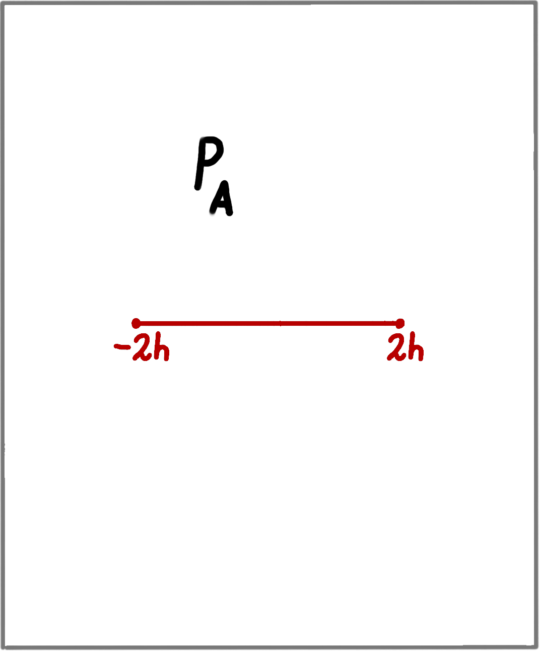
where and . Explicit expressions for , , as well as other matrices that appear throughout the main text are collected in Appendix A. The and have particularly simple analytic properties. must be a function with a short cut while must be a function with a long cut. We show these cuts in figure 1.


To study the Hagedorn temperature we need to twist the QSC. This implies that the Q-functions will have exponential asymptotics, as opposed to the polynomial asymptotic featured in the spectral problem. We can turn on a total of twists for . We will use the notation for the twists and for the twists. In the fully twisted case the asymptotics of for large , up to constants prefactors, are given by
| (3.7) |
where so that, for example, . Using (3.5) this translates in the fully twisted case into
| (3.8) |
with the identifications and . These pairings are a consequence of our choice of basis. We emphasize that (3.8) is valid only if we assume that all and are independent, otherwise one should include additional powers of .
Throughout this article, we will work in the symmetric sector. In this case we can identify
| (3.9) |
which enforces . Furthermore, in this sector we also have and .
3.1 The AdS4 Hagedorn QSC
We will from now on turn off all R-symmetry twists, thus setting . We fix the remaining twists to
| (3.10) |
The QSC naturally computes the Witten index. The factor of twists the trace in such a way to give instead the standard thermal partition function. Since there is no twisting of the -symmetry, the asymptotics of (3.7) picks up additional powers of , resulting in
| (3.11) |
and
| (3.12) |
The prefactors and satisfy the relations
| (3.13) |
Q-functions are not uniquely specified, rather we can transform our entire Q-system by acting on with linear transformations acting on either the or index. These transformations are usually called -rotations. These transformations are further restricted by 3.9 and by (3.11). We found it convenient to fix part of this freedom by imposing that
| (3.14) |
The Q-system also exibits parity symmetry, that is, after sending the Q-system is equivalent to the original one up to symmetry transformations. Explicitly
| (3.15) |
where we have used the notation . Here is a constant matrix while is in general a more complicated function with branch cuts. However, at large it is simply a constant. With our specific choice of gauge
| (3.16) |
The interesting part of these matrices is the distribution of non-zero entries rather than their exact value, which is dependent on normalization.
Since is a function with one short cut, we can parameterize it as
| (3.17) |
where is the Zhukovsky variable
| (3.18) |
and is an dependent integer. Using the parity symmetry and the asymptotic behavior described in (3.12) and (3.13), our ansatz in (3.17) takes the form
| (3.19a) | ||||
| (3.19b) | ||||
| (3.19c) | ||||
| (3.19d) | ||||
| (3.19e) | ||||
where powers of have been inserted so that . We have also used the -symmetry to eliminate a possible term in .
Finally, to close the QSC we supplement it with the so-called gluing conditions. As a function with short cuts is an upper half-plane analytic function with a ladder of cuts in the lower half-plane. In order to restore the long cut structure described previously, the analytic continuation of around the branch-points on the real axis, denoted by , must be a lower half-plane analytic function with a ladder of cuts in the upper half-plane. Luckily, we can easily construct such a function; namely . We demand that where is a matrix with periodicity . To fix the form of one should utilize the so-called -system as done in [20] for the spectral problem. We will not perform this analysis but rather argue the general form of from symmetry.
To constrain we use the asymptotic properties of . At we have that , and demand that the same ordering is true for at . This means that is upper-triangular. We also require that the ordering is preserved at which determines the exponential terms on the diagonal. The square-root cuts further add the restriction constraining the coefficients on the diagonal. Finally, we require that we do not add terms with different powers of in their asymptotics. Supplementing these restrictions with the weak coupling algorithm in the next section we found the matrix relation
| (3.20) |
The explicit form of depends on -rotations. For the choices described in this section we find that .
3.2 Perturbative solution
We now turn to the question of solving the constraints described in the previous section to obtain . In this section we consider the case at weak coupling, while in section 3.3 we consider strong coupling.
The first step in solving the ABJM QSC at weak coupling is to find the Q-system at zero coupling. At we expect that the Q-system should be fully regular, that is, should be polynomials in with exponential prefactors. To emphasize that we are now working at we write . The polynomial structure of the Q-functions at can be anticipated both from the knowledge of how to treat a twisted spin-chain using Q-functions [24] and from the Hagedorn QSC for AdSS5 [2]. To fix the exact form of the Q-functions we use that the ABJM QSC requires that [20]
as well as (3.4). In addition, we use the last -symmetry to impose the condition . This fixes all constants in the ansatz, leaving only the Hagedorn temperature to be fixed. We collect the explicit expressions for and in Appendix B.
To fix we compute using (3.20). Since and do not have cuts on the real axis, they must be regular functions around , that is
| (3.21) |
Imposing these relations at implies that , which we recognize as a solution to 33 3 The other solution to results in a negative temperature which we discard.. This is how the QSC finds the Hagedorn temperature at .
3.2.1 Going to higher orders
Techniques to solve the AdS4 QSC perturbatively at small coupling were developed in [25, 26], see also [27, 28, 29]. We will introduce a slightly different algorithm inspired by [30].
To describe our perturbative algorithm we start by rewriting (3.5) as
| (3.22) |
where . Let solve (3.22) to order and write
| (3.23) |
Using (3.4) we can solve for as
| (3.24) |
where
| (3.25) |
We then notice that , where does not contain any exponential prefactors. If we now choose the parameterization , then (3.24) becomes
| (3.26) |
where is given in (2.5). It is interesting to note that the additional signs appearing in (3.24) cancel against signs coming from .
The technology for solving equations of the type appearing in (3.26) was developed in [31, 32, 33]. Let us briefly recall the procedure. In the first iteration the source-term is , which from our parameterization is a Laurent polynomial in . For positive powers of it is straightforward to find as a polynomial in . For negative powers we need the twisted -function [30], which are functions without poles in the upper half-plane that solve
| (3.27) |
A formal expression is given by
| (3.28) |
Going to will require appearing on the right-hand side of (3.26). To solve equations of this type we need generalized twisted -functions, which are defined to satisfy
| (3.29) |
without poles in the upper half-plane and with and multi-indices. A formal expression for is
| (3.30) |
There is no need to introduce any more functions.
We note that there are also homogeneous solutions to (3.26). For example, when we can always add an -periodic function to and still solve (3.26). However, since by construction must have polynomial asymptotic behavior and cannot have poles in the upper-half plane, we can discard all homogeneous solutions except for constants. We thus write
| (3.31) |
with constants and a particular solution of (3.26) analytic in the upper half-plane, i.e. written in terms of -functions.
Thus, at each order in we can find as a function of -functions and with undetermined coefficients and . To fix these coefficients we follow the strategy in [2]. The first step is to construct using (3.9) and then impose (3.4). The second step is to verify the asymptotics (3.12) for . In our weak-coupling expansion
| (3.32) |
so that
| (3.33) |
It follows that , and all other functions containing , when expanded first in , will look like they contain higher powers of compared to (3.12). To make sure we still have the correct asymptotic behavior we solve [2]
| (3.34) |
3.2.2 The Hagedorn temperature to order
Using the algorithm described in section 3.2.1 we computed the Hagedorn temperature up to . The results are (using )
| (3.36) |
| (3.37) |
| (3.38) |
| (3.39) | ||||
| (3.40) | ||||
The analytic expression for is given in appendix C. All numerical estimates have been produced using DiffExp [34]. We see that our result for and agrees with the tree-level result of [7] and with the 2-loop calculation in [8], up to the aforementioned factor of . The results for and are new.
3.3 The numerical solution
To go to strong coupling we will resort to numerics. We will use standard methods first introduced for in [35] and implemented for the spectral problem of ABJM in [26] (see [36] for earlier numerical results from TBA). However, due to our exponential asymptotics we are forced to work slightly harder compared to the spectral problem, just as in [2].
3.3.1 The algorithm
We can also use the ansatz in (3.19) for the numerical solution. We only need to truncate all sums at so as to work with a finite number of unknowns. We then assume that for large that takes the form
| (3.42) |
where
and is an integer cut-off that satisfies . The large expansion of is constrained by the parity condition (3.15). Parity implies that are zero for odd and
| (3.43) |
for all . Note that the asymptotic form of in (3.16) is exact only up to exponentially suppressed terms at large u, so we can impose these parity constraints only on the large- expansion. As a gauge choice we also set
| (3.44) |
With these simplifications we can start solving order by order in the equation
| (3.45) |
At the leading five orders we solve for the following coefficients:
At this point it is convenient to solve a constraint coming from the restriction to the symmetric sector. Combining (3.9) and (3.4) leads to
| (3.46) |
Expanding this to order then fixes . Now we can go back to the main equation where we solve the next three orders:
After this, for all we can solve in order for:
The aim now is to check that glues correctly on the cut along the real line at the points
To get there we can start for each with from for a large odd positive integer and iterate using the equation
| (3.47) |
to get . Then we can compute and on opposite sides of the cut from
| (3.48) | ||||
| (3.49) |
with the gluing matrix from (3.20). We can also get from by sending the Zhukovsky variable to and thus get tilded versions of the above expressions by replacing with . Continuity through the cut implies that for the exact solution the function
| (3.50) |
is zero. We can then use the Levenberg-Marquardt algorithm [35] to find an approximate numerical solution.
3.3.2 The results
For weak coupling in the range we use the values , , and . For strong coupling with we use the same values. For we use , , and , for we use , , and , while for we increase and to , . We provide all results for the Hagedorn temperature at the above range of couplings in the ancillary files weak_h_squared.csv and strong_h.csv.
To check the numerical accuracy, we perturbed the result at and reran the algorithm 21 times at this same coupling to find that the Hagedorn temperature converged to the same value with an accuracy of 41 digits on all 21 runs. At the strong coupling point we did the same for 10 runs with perturbations of order and two runs at order to find results agreeing with 12 digit accuracy.
At weak the numerics agrees well with the perturbative solution of the QSC, as shown in figure 2. By fitting the numerical data with an even polynomial of order we match the first five terms with 15 digit precision against their exact values (3.40). In the plot we can observe the break down of the perturbative expansion in before . However the Padé approximation 3.41 fits well on the whole range of the weak coupling data.
At strong coupling we convert from to using (3.3) and fit against a series in negative powers in . To mitigate the errors choosing the correct range of data to fit on, we average over different values for the lowest value of and choose the range which gives the smallest estimated standard deviation for the leading fitted coefficient. We also vary how many orders we include in the series. This way we can check that the large asymptotics agrees with the string theory prediction at orders and . To get better numerical estimates for the subleading terms, we then subtract the exact string theory prediction for the two leading terms from our numerical data. Taking the mean of the resulting coefficients and estimating the standard deviation we find
| (3.51) |
We plot the numerical data and the fitted function in figure 3. We observe that the term matches the prediction in (2.23) within the error margins. If we now assume that the predicted value for this coefficient is correct, we can make a more precise estimate for the coefficient, and hence the value for , by refitting the curve. Our result is
| (3.52) |
In [1] we found that for AdS5 with slightly better numerical accuracy. This along with (3.52) leads us to conjecture that for general AdSd+1 the contribution from the zero-point shift is
| (3.53) |
4 Discussion
In this paper we computed the Hagedorn temperature at weak and strong coupling for ABJM using the QSC. At weak coupling we found the result up to eight loops, although there is theoretically no limit as to how high we could go. At strong coupling we found the Hagedorn temperature numerically in inverse powers of to four nontrivial orders in the expansion, showing that the last two terms are consistent with a conjectured form for the coefficients in the expansion.
Putting equations (2.22) and (3.52) together we observe a linear dependence on the dimension of the CFT for . However one could twist the -symmetries by turning on fugacities and explore how deformations related to the internal space affect the asymptotic behavior. In this case there is less symmetry in the QSC so the numerical calculations are slower. Perhaps recent work on numerical solutions of the QSC would be of use [37]. This investigation is in progress.
It would also be interesting to study the AdS3 case. The first correction in the expansion was already given in [38] and verified on the world-sheet in [16], with the next two terms given in (2.23) and (3.53). For AdS3 there is a conjectured form for the QSC [39, 40] and a TBA [41]. However, even for the spectral problem, it is not known how to take the AdS3 QSC to strong coupling with the present technology due to the novel analytic properties of the curve.
Acknowledgements
We thank Martijn Hidding for help with the numerical evaluation of polylogarithms. We also thank N. Bobev, N. Gromov, R. Tateo, G. Papathanasiou and M. Spradlin for discussions. This research is supported in part by the Swedish Research Council under grant #2020-03339 and by the National Science Foundation under Grant No. NSF PHY-1748958. Computations were done on a cluster provided by the National Academic Infrastructure for Supercomputing in Sweden (NAISS) at UPPMAX, partially funded by the Swedish Research Council under grant #2022-06725. S.E was partially supported by the European Research Council (ERC) under the European Union’s Horizon 2020 research and innovation programme (grant agreement No. 865075) EXACTC. J.A.M. thanks the KITP for hospitality during the beginning of this work.
Appendix A ABJM Conventions
We follow the conventions of [20]. We use for vector indices, and for the corresponding spinor indices. Relevant matrices pertaining to the are
| (A.1) | ||||||
| (A.2) |
The conventions are derived from the above conventions by identifying components 5 and 6. We use for the vector and for the spinor indices of the . Relevant matrices are
| (A.3) |
| (A.4) | ||||||
| (A.5) |
Appendix B Tree level solution
For the tree-level solution, , we find the following expressions for and
| (B.1) | ||||
| (B.2) |
Appendix C
Using from section 2.1 we find:
References
- [1] S. Ekhammar, J.A. Minahan and C. Thull, The asymptotic form of the Hagedorn temperature in planar super Yang-Mills, 2306.09883.
- [2] T. Harmark and M. Wilhelm, Solving the Hagedorn temperature of AdS5/CFT4 via the Quantum Spectral Curve: chemical potentials and deformations, JHEP 07 (2022) 136 [2109.09761].
- [3] O. Aharony, O. Bergman, D.L. Jafferis and J. Maldacena, N=6 superconformal Chern-Simons-matter theories, M2-branes and their gravity duals, JHEP 10 (2008) 091 [0806.1218].
- [4] T. Harmark and M. Wilhelm, Hagedorn Temperature of AdS5/CFT4 via Integrability, Phys. Rev. Lett. 120 (2018) 071605 [1706.03074].
- [5] T. Harmark and M. Wilhelm, The Hagedorn temperature of AdS5/CFT4 at finite coupling via the Quantum Spectral Curve, Phys. Lett. B 786 (2018) 53 [1803.04416].
- [6] E.Y. Urbach, String Stars in Anti De Sitter Space, JHEP 04 (2022) 072 [2202.06966].
- [7] T. Nishioka and T. Takayanagi, On Type IIA Penrose Limit and N=6 Chern-Simons Theories, JHEP 08 (2008) 001 [0806.3391].
- [8] G. Papathanasiou and M. Spradlin, The Morphology of N=6 Chern-Simons Theory, JHEP 07 (2009) 036 [0903.2548].
- [9] F. Bigazzi, T. Canneti and A.L. Cotrone, Higher Order Corrections to the Hagedorn Temperature at Strong Coupling, 2306.17126.
- [10] B.I. Zwiebel, Two-loop Integrability of Planar N=6 Superconformal Chern-Simons Theory, J. Phys. A 42 (2009) 495402 [0901.0411].
- [11] J.A. Minahan, W. Schulgin and K. Zarembo, Two loop integrability for Chern-Simons theories with N=6 supersymmetry, JHEP 03 (2009) 057 [0901.1142].
- [12] O. Bergman and S. Hirano, Anomalous radius shift in AdS(4)/CFT(3), JHEP 07 (2009) 016 [0902.1743].
- [13] K. Sugiyama and K. Yoshida, Type IIA string and matrix string on PP wave, Nucl. Phys. B 644 (2002) 128 [hep-th/0208029].
- [14] S.-j. Hyun and H.-j. Shin, N=(4,4) type 2A string theory on PP wave background, JHEP 10 (2002) 070 [hep-th/0208074].
- [15] S.-j. Hyun, J.-D. Park and S.-H. Yi, Thermodynamic behavior of IIA string theory on a pp wave, JHEP 11 (2003) 006 [hep-th/0304239].
- [16] F. Bigazzi, T. Canneti and W. Mück, Semiclassical Quantization of the Superstring and Hagedorn Temperature, 2306.00588.
- [17] A. Cavaglià, D. Fioravanti, N. Gromov and R. Tateo, Quantum Spectral Curve of the 6 Supersymmetric Chern-Simons Theory, Phys. Rev. Lett. 113 (2014) 021601 [1403.1859].
- [18] D. Bombardelli, D. Fioravanti and R. Tateo, TBA and Y-system for planar AdS(4)/CFT(3), Nucl. Phys. B 834 (2010) 543 [0912.4715].
- [19] N. Gromov and F. Levkovich-Maslyuk, Y-system, TBA and Quasi-Classical strings in AdS(4) x CP3, JHEP 06 (2010) 088 [0912.4911].
- [20] D. Bombardelli, A. Cavaglià, D. Fioravanti, N. Gromov and R. Tateo, The full Quantum Spectral Curve for , JHEP 09 (2017) 140 [1701.00473].
- [21] N. Gromov and G. Sizov, Exact Slope and Interpolating Functions in N=6 Supersymmetric Chern-Simons Theory, Phys. Rev. Lett. 113 (2014) 121601 [1403.1894].
- [22] N. Bobev, J. Hong and V. Reys, Large N partition functions of the ABJM theory, JHEP 02 (2023) 020 [2210.09318].
- [23] N. Bobev, J. Hong and V. Reys, Large N Partition Functions, Holography, and Black Holes, Phys. Rev. Lett. 129 (2022) 041602 [2203.14981].
- [24] V. Kazakov, S. Leurent and D. Volin, T-system on T-hook: Grassmannian Solution and Twisted Quantum Spectral Curve, JHEP 12 (2016) 044 [1510.02100].
- [25] L. Anselmetti, D. Bombardelli, A. Cavaglià and R. Tateo, 12 loops and triple wrapping in ABJM theory from integrability, JHEP 10 (2015) 117 [1506.09089].
- [26] D. Bombardelli, A. Cavaglià, R. Conti and R. Tateo, Exploring the spectrum of planar AdS4/CFT3 at finite coupling, JHEP 04 (2018) 117 [1803.04748].
- [27] R.N. Lee and A.I. Onishchenko, ABJM quantum spectral curve and Mellin transform, JHEP 05 (2018) 179 [1712.00412].
- [28] R.N. Lee and A.I. Onishchenko, Toward an analytic perturbative solution for the ABJM quantum spectral curve, Teor. Mat. Fiz. 198 (2019) 292 [1807.06267].
- [29] R.N. Lee and A.I. Onishchenka, ABJM quantum spectral curve at twist 1: algorithmic perturbative solution, JHEP 11 (2019) 018 [1905.03116].
- [30] N. Gromov, F. Levkovich-Maslyuk and G. Sizov, Pomeron Eigenvalue at Three Loops in 4 Supersymmetric Yang-Mills Theory, Phys. Rev. Lett. 115 (2015) 251601 [1507.04010].
- [31] S. Leurent and D. Volin, Multiple zeta functions and double wrapping in planar SYM, Nucl. Phys. B 875 (2013) 757 [1302.1135].
- [32] C. Marboe and D. Volin, Quantum spectral curve as a tool for a perturbative quantum field theory, Nucl. Phys. B 899 (2015) 810 [1411.4758].
- [33] N. Gromov and F. Levkovich-Maslyuk, Quantum Spectral Curve for a cusped Wilson line in SYM, JHEP 04 (2016) 134 [1510.02098].
- [34] M. Hidding, DiffExp, a Mathematica package for computing Feynman integrals in terms of one-dimensional series expansions, Comput. Phys. Commun. 269 (2021) 108125 [2006.05510].
- [35] N. Gromov, F. Levkovich-Maslyuk and G. Sizov, Quantum Spectral Curve and the Numerical Solution of the Spectral Problem in AdS5/CFT4, JHEP 06 (2016) 036 [1504.06640].
- [36] F. Levkovich-Maslyuk, Numerical results for the exact spectrum of planar AdS4/CFT3, JHEP 05 (2012) 142 [1110.5869].
- [37] N. Gromov, A. Hegedus, J. Julius and N. Sokolova, Fast QSC Solver: tool for systematic study of N=4 Super-Yang-Mills spectrum, 2306.12379.
- [38] E.Y. Urbach, The black hole/string transition in AdS3 and confining backgrounds, 2303.09567.
- [39] S. Ekhammar and D. Volin, Monodromy bootstrap for SU(2—2) quantum spectral curves: from Hubbard model to AdS3/CFT2, JHEP 03 (2022) 192 [2109.06164].
- [40] A. Cavaglià, N. Gromov, B. Stefański, Jr., Jr. and A. Torrielli, Quantum Spectral Curve for AdS3/CFT2: a proposal, JHEP 12 (2021) 048 [2109.05500].
- [41] S. Frolov and A. Sfondrini, Mirror thermodynamic Bethe ansatz for AdS3/CFT2, JHEP 03 (2022) 138 [2112.08898].