Self-Consuming Generative Models Go MAD
Abstract
Seismic advances in generative AI algorithms for imagery, text, and other data types has led to the temptation to use synthetic data to train next-generation models. Repeating this process creates an autophagous (“self-consuming”) loop whose properties are poorly understood. We conduct a thorough analytical and empirical analysis using state-of-the-art generative image models of three families of autophagous loops that differ in how fixed or fresh real training data is available through the generations of training and in whether the samples from previous-generation models have been biased to trade off data quality versus diversity. Our primary conclusion across all scenarios is that without enough fresh real data in each generation of an autophagous loop, future generative models are doomed to have their quality (precision) or diversity (recall) progressively decrease. We term this condition Model Autophagy Disorder (MAD), making analogy to mad cow disease.
1 Introduction
1.1 Generative models are training on synthetic data from generative models
Due to rapid advances in generative artificial intelligence (AI), synthetic data of all kinds is rapidly proliferating. Publicly available generative models have not only revolutionized the image, audio, and text domains [2, 3, 4, 5, 6, 7, 8, 9], but they are also starting to impact the creation of videos, 3D models, graphs, tables, software, and even websites [10, 11, 12, 13, 14, 15]. Companies like Google, Microsoft, and Shutterstock are incorporating generative models into their consumer services, and the output from these services and popular generative models like Stable Diffusion [2] (for images) and ChatGPT [16] (for text) tend to end up on the Internet. The world is racing towards a future that is best summarized by a comment overheard at the 2022 ICLR conference: “There will soon be more synthetic data than real data on the Internet.”
Since the training datasets for generative AI models tend to be sourced from the Internet, today’s AI models are unwittingly being trained on increasing amounts of AI-synthesized data. Indeed, Figure 2 demonstrates that the popular LAION-5B dataset [17], which is used to train state-of-the-art text-to-image models like Stable Diffusion [2], contains synthetic images sampled from several earlier generations of generative models. Formerly human sources of text are now increasingly created by generative AI models, from user reviews [18] to news websites [15], often with no indication that the text is synthesized [19]. As the use of generative models continues to grow rapidly, this situation will only accelerate.
Moreover, throwing caution to the wind, AI-synthesized data is increasingly used by choice in a wide range of applications [20, 21, 22, 23, 9, 24], for a number of reasons. First, it can be much easier, faster, and cheaper to synthesize training data rather than source real-world samples, particularly for data-scarce applications. Second, in some situations synthetic data augmentation has been found empirically to boost AI system performance [25, 26, 27]. Third, synthetic data can protect privacy [27, 28, 29] in sensitive applications like medical imaging or medical record aggregation [29, 30]. Fourth, and most importantly, as deep learning models become increasingly enormous, we are simply running out of real data on which to train them [31, 32, 33]. Interestingly, not only have practitioners begun deliberately training AI systems on synthetic data, but also the human annotators who provide gold-standard annotations for supervised learning tasks are increasingly using generative models to increase their productivity and income [34].
The witting or unwitting use of synthetic data to train generative models departs from standard AI training practice in one important respect: repeating this process for generation after generation of models forms an autophagous (“self-consuming”) loop. As Figure 3 details, different autophagous loop variations arise depending on how existing real and synthetic data are combined into future training sets. Additional variations arise depending on how the synthetic data is generated. For instance, practitioners or algorithms will often introduce a sampling bias by manually “cherry picking” synthesized data to trade off perceptual quality (i.e., the images/texts “look/sound good”) vs. diversity (i.e., many different “types” of images/texts are generated). The informal concepts of quality and diversity are closely related to the statistical metrics of precision and recall, respectively [39]. If synthetic data, baised or not, is already in our training datasets today, then autophagous loops are all but inevitable in the future.
No matter what the training set makeup or sampling method, the potential ramifications of autophagous loops on the properties and performance of generative models is poorly understood. In one direction, repeated training with synthetic data might progressively amplify the biases and artifacts present in any generative model. We hypothesize that synthetic data contains fingerprints of the generator architecture (e.g., convolutional traces [40] or aliasing artifacts [41]) that may be reinforced by self-consuming generators. To illustrate this, in Figure 1 we present samples generated by StyleGAN-2 generative models after repeated training on synthetic data. Each generation results in a progressive amplification of cross-hatching artifacts, which are reminiscent of aliasing in StyleGAN-2 as suggested by [41]. In another direction, autophagous loops featuring generative models tuned to produce high quality syntheses at the expense of diversity (such as [1, 42]) might progressively dilute the diversity of the data on the Internet. The closest exploration to this potential outcome has been the issue of diversity exposure in recommender systems, where some studies have shown that, if a recommendation system is tuned for maximum click rate, then an echo chamber results, and users lose exposure to diverse ideas. [43, 44, 45, 46, 47]. Other studies have shown that, subject to the recommendation logic, the echo chamber effect might not be as pronounced [48] and could be on par with that produced by human curators [49]. Exactly how the above and other unintended consequences could emerge from autophagous loops deserves thorough consideration and study.
For analogies and cautionary tales, one may turn to mathematics and biology. In the language of mathematics, at one extreme, an autophagous loop is a contraction mapping that collapses to a single, boring, point, while at the other extreme it is an unstable positive feedback loop that diverges into bedlam. Biology provides a particularly apt “seemed like a good idea at the time” in the practice of feeding cattle with the remains (including brains) of other cattle. The resulting autophagous loop led to mad cow disease [50], a fatal neurodegenerative disease that eventually spread to humans before a massive intervention brought it under control. Lest an analogous malady disrupt the AI future, and to coin a term, it seems prudent to understand what can be done to prevent generative models from developing Model Autophagy Disorder (MAD).
1.2 Contributions
In this paper, we conduct a careful theoretical and empirical study of AI augophagy from the perspective of generative image models. While we focus on image data for concreteness, the concepts developed herein apply to any data type, including text and Large Language Models (LLMs). This paper is an elaboration of work initially published in [51, 52]; while it was being finalized, we became aware of contemporaneous work in [53] and [54, 55] that explores certain aspects of our more general theory. We will discuss the results of these papers in context below.
Let us summarize the three key contributions and findings that lie at the focus of this paper:
Realistic models for autophagous loops.
We propose three families of increasingly complex self-consuming training loops that realistically model the way real and synthetic data are combined into autophagous training datasets for generative models (recall Figure 3):
- •
The fully synthetic loop, wherein the training dataset for each generation’s model consists solely of synthetic data sampled from previous generations’ models. This case arises in practice, for example, when iteratively fine-tuning a generative model on its own high-quality outputs (e.g., [56]). We show below in Section 3 that in this case either the quality (precision) or the diversity (recall) of the generative models decreases over generations.
- •
The synthetic augmentation loop, wherein the training dataset for each generation’s model consists of a combination of synthetic data sampled from previous generations’ models plus a fixed set of real training data. This case arises in practice, for example, in model “self-improvement,” where a model’s training data are augmented with synthetic data from some other models (e.g., [57]). We show below in Section 4 that in this case fixed real training data only delays the inevitable degradation of the quality or diversity of the generative models over generations.
- •
The fresh data loop, wherein the training dataset for each generation’s model consists of a combination of synthetic data sampled from previous generations’ models plus a fresh set of real training data. This case models, for example, the standard practice where training datasets are acquired by scraping the Internet, which will find both real and synthetic data (recall Figure 2). We show below in Section 5 that in this case, with enough fresh real data, the quality and diversity of the generative models do not degrade over generations.
The bottom line across all three autophagous loop models is that without enough fresh real data each generation, future generative models are doomed to go MAD.
Sampling bias plays a key rôle in autophagous loops.
Users of generative models tend to manually curate (“cherry-pick”) their synthetic data, preferring high-quality samples and rejecting low-quality ones. Moreover, state-of-the-art generative models typically feature controllable parameters that can increase synthetic quality at the expense of diversity [58, 42]. We demonstrate that the sampling biases induced through such quality-diversity (precision-recall) trade-offs have a major impact on the behavior of an autophagous training loop. Specifically, we show that, without sampling bias, autophagy can lead to a rapid decline of both quality and diversity, whereas, with sampling bias, quality can be maintained but diversity degrades even more rapidly.
Autophagous loop behaviors hold across a variety of generative models and datasets.
In addition to our analytical and empirical studies on simple multivariate Gaussian and Gaussian mixture models, we demonstrate in the main text and Appendix that our main conclusions hold across a variety of generative models, including Denoising Diffusion Probabilistic Models (DDPM) [59], StyleGAN-2 [58], WGAN [60], and Normalizing Flows [61] trained on a number of image datasets, including MNIST [62] and FFHQ [63].
This paper is organized as follows. In Section 2, we rigorously define the concept of an autophagous loop, explain our universal biased sampling parameter for generative models, and define the metrics we will use to measure the quality and diversity of a generative model. Then, in Sections 3, 4, and 5, we study the fully synthetic loop, synthetic augmentation loop, and fresh data loop models, respectively. We conclude with a discussion in Section 6. We report on the results of numerous additional experiments in various Appendices.
2 Self-consuming generative models
Modern generative models have advanced rapidly in their ability to synthesize realistic data (signals, images, videos, text, and beyond) given a finite collection of training samples from a reference (target) probability distribution . As generative models have proliferated, the datasets for training new models have unwittingly (see [17] and Figure 2) or wittingly [64, 65, 57, 66, 67] begun to include increasing amounts of synthetic data in addition to “real world” samples from (recall Figure 3).11 1 While the term “real” implies non-synthetic data from the “real-world” (e.g., a photographic image of a natural scene), in general, real data is any data drawn from the reference distribution . In this section, we propose a hierarchy of increasingly realistic models for this autophagy (self-consuming) phenomenon that will enable us to draw a number of conclusions about the potential ramifications for generative modeling as synthetic training data proliferates.
2.1 Autophagous processes
Consider a sequence of generative models , where the goal is to train each model to approximate a reference probability distribution . At each generation , the model is trained from scratch on the dataset comprised of both real data samples drawn from and synthetic data samples produced by already trained generative model(s). The first-generation model is trained on purely real data, i.e., .
Definition.
An autophagous generative process is a sequence of distributions where each generative model is trained on data that includes samples from previous models .
In this work, we study cases where such a process deteriorates (goes “MAD”) over time. Let denote some distance metric on distributions.
Definition.
A MAD generative process is a sequence of distributions that follows a random walk such that increases with .
Claim.
Under mild conditions, an autophagous generative process is a MAD generative process.
By studying whether a sequence of generative models forms a MAD generative process, we can gain insights into the potentially detrimental effects of training generative models on synthetic data.
2.2 Variants of autophagous processes
In this paper, we study three realistic autophagous mechanisms, each of which includes synthetic data and potentially real data in a feedback loop (recall Figure 3). We now add some additional details to the descriptions from Section 1.2:
- •
The fully synthetic loop: In this scenario, each model for is trained exclusively on synthetic data sampled from models from previous generations, i.e., .
- •
The synthetic augmentation loop: In this scenario, each model for is trained on a dataset consisting of a fixed set of real data sampled from plus synthetic data from models from previous generations.
- •
The fresh data loop: In this scenario, each model for is trained on a dataset consisting of a fresh set of real data drawn independently from plus synthetic data from models from previous generations.
2.3 Biased sampling in autophagous loops
While the above three autophagous loops realistically mimic real-world generative model training scenarios that involve synthetic data, it is also critical to consider how each generation’s synthetic data is produced. In particular, not all synthetic samples from a generative model will have the same level of fidelity to the training distribution, or “quality.” Consequently, in many applications (e.g., art generation), practitioners “cherry-pick” synthetic samples based on a manual evaluation of perceived quality. It can be argued that most of the synthetic images that one can find on the Internet today are to some degree cherry-picked based on human evaluation of perceptual quality. Therefore, it is critical that this notion be included in the modeling and analysis of autophagous loops.
In our modeling and analysis, we implement cherry-picking via the biased sampling methods that are commonly used in generative modeling practice, such as truncation in BigGAN and StyleGAN [38, 58], guidance in diffusion models [42], polarity sampling [68], and temperature sampling in large language models [7]. These techniques assume that the data manifold is better approximated in the higher density regions of the learned distribution. By biasing a generative model’s synthetic samples to be drawn from parts of the learned generative model distribution that are closer to its modes, these methods increase sample fidelity or quality by trading off the variety or diversity of the synthesized data [68].
We employ a number of generative models in our experiments below; each has a unique controllable parameter to increase sample quality. We unify these parameters in the universal sampling bias parameter , where corresponds to unbiased sampling and corresponds to sampling from the modes of the generative distribution with zero variance. The exact interpretation of differs across various models, but in general synthetic sample quality will increase and diversity decrease as is decreased from . Below we provide specific definitions for for the various generative models we consider in this paper:
- •
Gaussian model: Our theoretical analysis and simplified experiments use a multivariate Gaussian toy model. To implement biased sampling at generation , we estimate the mean and covariance of the training data and then sample from the distribution . As decreases, we draw samples closer to the mean .
- •
Generative adversarial network: In our StyleGAN experiments, we use the truncation parameter to increase sampling quality. Style-based generative networks employ a secondary latent space called the style-space. When using truncation during inference, latent vectors in the style-space are linearly interpolated towards the mean of the style-space latent distribution. We denote the truncation factor by ; as is decreased from , samples are drawn closer to the mean of the style-space distribution.
- •
Denoising diffusion probabilistic model (DDPM): For conditional diffusion models, we use classifier-free diffusion guidance [42] to bias the sampling towards higher probability regions. We use conditioning dropout during training to enable classifier-free guidance. We define the bias parameter in terms of the guidance factor from [42] as . When , the network acts as a conventional conditional diffusion model with no guidance. As decreases, the diffusion model samples more closely to the modes of the unconditional distribution, producing higher-quality samples.
2.4 Metrics for MADness
Ascertaining whether an autophagous loop has gone MAD or not (recall Definition Definition) requires that we measure how far the synthesized data distribution has drifted from the true data distribution over the generations . We use the notion of the Wasserstein distance (WD) as implemented by the Fréchet Inception Distance (FID) for this purpose. We will also find the standard concepts of precision and recall useful for making rigorous the notions of quality and diversity, respectively.
Wasserstein distance (WD), or earth mover’s or optimal transport distance [69], measures the minimum work required to move the probability mass of one distribution to another. Computing the Wasserstein distance between two datasets (e.g., real and synthetic images) is prohibitively expensive. As such, standard practice employs the Fréchet Inception Distance (FID) [70] as an approximation, which calculates the Wasserstein-2 distance between inception feature distributions of real and synthetic images.
Precision quantifies the portion of synthesized samples that are deemed high quality or visually appealing. We use precision as an indicator of sample quality. We compute precision by calculating the fraction of synthetic samples that are closer to a real data example than to their -th nearest neighbor [39]. We use in all experiments.
Recall estimates the fraction of samples in a reference distribution that are inside the support of the distribution learned by a generative model. High recall scores suggest that the generative model captures a large portion of diverse samples from the reference distribution. We compute recall in a manner similar to precision [39]. Given a set of synthetic samples from the generative model, we calculate the fraction of real data samples that are closer to any synthetic sample than its -th nearest neighbor.
2.5 Related work
Contemporaneous work on feedback loops in generative modeling has explored certain aspects of our more general theory that confirm our main conclusions.
In [53], the authors show that, for the fully synthetic loop without sampling bias, variational autoencoders (VAE) and Gaussian mixture models result in MAD generative processes. They also investigate training loops resembling the synthetic augmentation loop and fresh data loop, again without sampling bias, on LLMs. However, they take a slightly different approach from ours by fine-tuning the generative model with synthetic data instead of training from scratch. Their studies demonstrate that both the synthetic augmentation loop and fresh data loop can result in a decline in performance in fine-tuned LLMs over generations.
In [54], the authors focus on the fully synthetic loop with sampling bias by utilizing a diffusion model with guidance and report that it prevents a drop in image quality. In [55], the same authors show that a synthetic augmentation loop containing a Denoising diffusion implicit model (DDIM) [71] without sampling bias leads to poor performance over generations. The results in [53, 54, 55] report some certain facets of a MAD generative process that align with our analytical and experimental results.
3 The fully synthetic loop: Training exclusively on synthetic data leads to MADness
Here we thoroughly analyze the fully synthetic loop, wherein each model is trained using synthesized data from the previous generations. We focus on the the inter-generational propagation of non-idealities resulting from estimation errors and sampling biases. Specifically, we pinpoint the primary source of these non-idealities and characterize the convergence of the loop. The simplicity of the fully synthetic loop means that it does not accurately reflect the reality of generative modeling practice. However, one specific example of this case is when generative models are fine-tuned on their own high-quality outputs [56]. Nevertheless, this loop is in a sense the worst case and so offers valuable insights that can be extrapolated to the more practical autophagous loops discussed in subsequent sections.
Our analysis and experiments below support our main conclusion for the fully synthetic loop, which can be summarized as either the quality (precision) or the diversity (recall) of the generative models decreases over generations.
3.1 Warm up: Gaussian data and martingales
In this section, we focus the fully synthetic loop and a Gaussian reference distribution and show that its martingale nature makes it a MAD generative process.
Consider a reference (real data) distribution for some and , and let our generation process also be Gaussian: . At each time , we sample vectors from with sampling bias ; that is, we draw . We then use these vectors to construct the unbiased sample mean and covariance to fit the next model :
| (1) |
In this case, we also know the distributions of these parameters. We have and , with being the Wishart distribution. The process satisfies
| (2) |
which means that and are martingale and supermartingale processes, respectively [72]. Due to the uncertainty in estimation of due to the limited sample size, is a Gaussian random walk that will tend to drift from over time, randomly biasing the distribution estimate. Moreover, due to being a bounded supermartingale, the covariance is guaranteed to converge to zero. The proof of the following result can be found in Appendix A.
Proposition.
For the random process defined in Equation 1, for any , we have
That is, when fitting a distribution to data sampled from that distribution repeatedly, not only should we expect some modal drift because of the random walk in (reduction in quality), but we will also inevitably experience a collapse of the variance (vanishing of diversity).
The key idea to takeaway from this is that these effects—the random walk and the variance collapse—are solely due to the estimation error of fitting the model parameters using random data. Importantly, this result holds true even when there is no sampling bias (i.e., ). The magnitudes of the steps of the random walk in are determined by two main factors: the number of samples and the covariance . Unsurprisingly, the larger the , the smaller the steps of the random walk, since there will be less estimation error. This will also slow the convergence of to . Meanwhile, can be controlled using a sampling bias factor . The smaller the choice of , the more rapidly will converge to zero, stopping the random walk of (as illustrated in 17). Thus, the sampling bias factor provides a trade-off to preserve quality at the expense of diversity.
It was recently shown in related work [53] that the expected Wasserstein-2 metric , or distributional distance, is increasing for this process. This supports our conclusion that is a MAD generative process.
3.2 Experimental setups for the fully synthetic loop
Here we simulate the fully synthetic loop using two widely used types of deep generative models. Recall that the fully synthetic loop first requires training an initial model with a fully real dataset containing samples. In our experiments, all subsequent models are trained using only synthetic samples from the immediately preceding model , where each synthetic sample is produced with sampling bias . Our primary experiments are organized as follows:
Generation 2

Generation 5

Generation 10

Generation 20

- •
Denoising diffusion probabilistic model: We use a conditional DDPM [59] with diffusion time steps and train it on the MNIST dataset. In this experiment the synthetic dataset is only sampled from the previous generation , with for .22 2 For all MNIST DDPM experiments we use features extracted by LeNet [73] instead of the Inception network for calculating the Wasserstein distance, since numerical digits do not fall into the domain of natural images. For consistency we also use the term “FID” for the MNIST results.
- •
Generation 2

Generation 5

Generation 10

Generation 20

3.3 Without sampling bias, the quality of synthetic data decreases
Let us first investigate the fully synthetic loop without any sampling bias (). In higher-dimensional multimodal settings, we use precision and recall to measure synthetic quality and diversity (as supported in Section B.2). Figure 4 illustrates the FID, precision, and recall for each generation of model. In the absence of sampling bias, the distribution of synthetic data undergoes a random walk deviating from the original distribution, caused by the finite sample size of any given training dataset. Consequently, as the generations progress, both the precision and recall of models decrease, while the FID metric exhibits a steady increase. Figure 13 confirms that these trends in FID, precision, and recall continue until eventually saturating.
As the generations advance, the synthetic data distribution eventually diverges completely from the true distribution, resulting in a synthetic distribution with little resemblance to real data. This lack of realism is reflected in how the precision and recall of each model eventually drop to zero (see Figure 16 in the appendix for more MNIST DDPM generations), despite having a non-zero variance.
Figure 5 visualizes this process using the MNIST dataset. We employ the t-distributed Stochastic Neighbor Embedding (t-SNE) [74] to reduce the dimensionality of both the real and synthetic MNIST datasets at each generation. The visualization reveals that over time, the modes of the synthetic data progressively move away from the real distribution. Despite being produced by a conditional model, these modes eventually merge together, forming a unified, larger mode of data. This gradual divergence away from the modes of real data contributes to the decrease in precision and recall, and consequently, the increase in FID, resulting in a MAD generative process.
3.4 With biased sampling, quality can increase, but diversity will decrease rapidly
In this section, we present the results obtained with sampling bias (). Figure 6 shows the FID, precision, and recall of models at each generations. We see that involvement of sampling bias results in increase of precision in generations; however, it causes a faster drop of recall compared to the case without sampling bias, which all together results in an increase in FID, making it a MAD generative process.
The visualization of fully synthetic loop with sampling bias is shown in Figure 7. In the presence of sampling bias, the movement of modes of synthetic data is confined within the support of the real data, unlike the case without sampling bias where the modes merge together. However, the variance of synthetic data rapidly decreases, resulting in very limited diversity within the synthetic data.
We provide more experiments for the fully synthetic loop with Gaussian mixture models, WGAN [60], and Normalizing Flows [61] in Appendix B that all result in MAD generative processes.
4 The synthetic augmentation loop: Fixed real training data may delay but not prevent MADness
Although the analysis is tractable in the fully synthetic loop, there is little reason to believe that the it will be representative of real practice. In training real generative models, practitioners will always prefer to use at least some real data when available. In this section, we explore the synthetic augmentation loop, in which the training data consists of a fixed real dataset that is progressively augmented with synthetic data.
We motivate the synthetic augmentation loop with the recent practice of using generative models for augmenting datasets in classification tasks, which has shown promising results thanks to advancements in generative models [26, 27]. However, the impact of data augmentation using generative models is still not fully understood. While increasing the volume of training data generally improves the performance of machine learning models, when synthetic samples are introduced into the dataset, there is uncertainty due to the potential deviation of synthetic data from the true distribution of data. Even a small discrepancy can impact the model’s fidelity to the real-world data distribution. As we demonstrate, the presence of the fixed real dataset is not enough to prevent this loop from producing a MAD generative process.
Our experiments below support our main conclusion for the synthetic augmentation loop, which can be summarized as fixed real training data only delays the inevitable degradation of the quality or diversity of the generative models over generations.
4.1 Experimental setups for the synthetic augmentation loop
Here we simulate the synthetic augmentation loop using the same deep generative models and experimental conditions as in Section 3.2. Recall that we first require training an initial model with a fully real dataset of samples. All subsequent models are trained using synthetic samples from the previous model(s) and all of the original samples used to train . Note that each synthetic sample is always produced with sampling bias . Our experiments are organized as follows:
- •
Denoising diffusion probabilistic model: We use a conditional MNIST DDPM [59] with diffusion time steps. In this experiment the synthetic dataset is only sampled from the previous generation with sampling bias , and for all . The original real MNIST dataset is also available at every generation: and for all .
- •
Generative adversarial network: We use an unconditional StyleGAN2 architecture [58] trained on the FFHQ-128128 dataset [63]. Like the StyleGAN experiment in Section 3.2, at each generation we sample images with no sampling bias () from the immediately preceding model . However, now the synthetic dataset includes all the previously generated samples (not just the ones from generation ), producing a synthetic data pool of size that grows linearly with respect to . The real FFHQ dataset is always present at every generation: and for every generation .
4.2 A fixed real dataset only slows generative model degradation
Here we show that keeping the original real dataset in the synthetic augmentation loop only slows the malignant effects of the fully synthetic loop instead of preventing them. Figure 8 shows how keeping the full FFHQ dataset in a StyleGAN synthetic augmentation loop still produces the same symptoms as the fully synthetic loop: the overall distance from the real dataset (FID) increases, while the quality (precision) and diversity (recall) of synthetic samples still decrease in the absence of sampling bias. In fact, in Appendix F we see the same artifacts appear as in Figure 1 and Appendix C. Unlike all our other experiments, we opt for a linearly growing pool of synthetic data in the StyleGAN synthetic augmentation loop to simulate: (a) whether access to previous generations’ synthesized samples could help future generations learn, and (b) what could happen to a domain of data (e.g., the Internet) in a fresh data loop with almost no newly sampled data points and unlimited access to previous generations’ samples.
Additionally, Figure 9 depicts how the sampling bias affects the synthetic augmentation loop in much the same way as it did the fully synthetic loop: the overall distance from the real dataset (FID) still increases (albeit more slowly), while the synthetic quality (precision) can increase, but only at the cost of accelerated losses in synthetic diversity (recall). Naturally, some values of are better than others at mitigating losses in FID and precision (for example, in Figure 9).
5 The fresh data loop: Fresh real data can prevent MADness
The most elaborated our autophagous loop models enable new training data to come from two sources: fresh real data from the reference distribution, and synthetic data from previously trained generative models. A clear instance of this can be observed in the LAION-5B dataset [17], which already incorporates images from generative models like Stable Diffusion [2] (recall Figure 2).
To understand the evolution of the generative models trained in this way, in this section, we investigate the fresh data loop, which takes the synthetic augmentation loop one step further by incorporating new fresh samples of real data at each iteration. Concretely, we imagine that the real data samples constitute only a fraction of the available data pool (e.g., a training dataset or the Internet) with the remaining fraction being synthetic data from generative models. When we independently sample data points from such a training data set to train a generative model in the th generation, there will be data points that originate from the real distribution and synthetic data points.
In this context, we observe in our experiments below that the presence of fresh data samples fortunately mitigate the development of a MAD generative process; i.e., fresh new data helps keep the generative distribution somewhat close to the reference distribution instead of undergoing a purely random walk. However, we still observe some alarming phenomena. First, we find that—regardless of the performance of early generations—the performance of later generations converges to a point that depends only on the amounts of real and synthetic data in the training loop. Second, we find that, while limited amounts of synthetic data can actually improve the distributional estimate in the fresh data loop—since synthetic data effectively transfers previously used real data to subsequent generations and increases the effective dataset size—too much synthetic data can still dramatically decrease the performance of the distributional estimate.
Our analysis and experiments below support our main conclusion for the fresh data loop:, which can be summarized as with enough fresh real data, the quality and diversity of the generative models do not degrade over generations.
5.1 Experimental setups for fresh data loop
As in previous autophagous loop variants, we assume that all models are initially trained solely on real samples, with the number of real samples denoted here as . In subsequent generations (i.e., for ) the generative models are trained with a fixed number of real samples, denoted as , and a fixed number of synthetic samples, denoted by . In the fresh data loop, the dataset is independently sampled from the reference probability distribution , while the dataset is sampled exclusively from the previous generation , with a sampling bias represented as .
Throughout the remainder of this section, we simulate the fresh data loop using different values for , and , considering the following models and their associated reference probabilities:
- •
Gaussian modeling: We consider a normal reference distribution with a dimension of . For modeling the Gaussian distribution, we utilize an unbiased moment estimation approach, as described in Equation 1.
- •
Denoising diffusion probabilistic model: We use a conditional DDPM [59] with diffusion time steps. We consider the MNIST dataset as our reference distribution.
The Gaussian example enables examination of the fresh data loop in greater detail, especially in the asymptotic regime. Meanwhile, our MNIST DDPM example demonstrates the impact of fresh data loop on more realistic dataset and model.
5.2 Initial models will eventually be forgotten in the fresh data loop
Here we investigate the impact of the initial model in the fresh data loop. We begin by training the first generative model on samples, and train the remaining generative models with samples, where synthetic samples are synthesized with bias . Figure 10 summarizes the results for this experiment.
Interestingly, for both model types, we found that the Wasserstein distance/FID converged to a limiting value after a few iterations, and that this limiting value was independent of . In other words, for a given combination of model type and ground truth distribution , we observed that the final outcome only depends on , that is,
| (3) |
Thus, the initial model’s influence diminished throughout the process, with only the aforementioned parameters having an impact on the final result.
In the context of autophagy, this point brings some hope: with the incorporation of fresh new data at each generation, there is not necessarily an increase in as grows. Thus, the fresh data loop can prevent a MAD generative process.
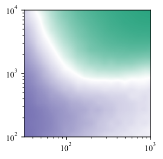
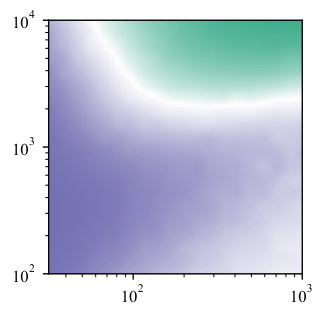
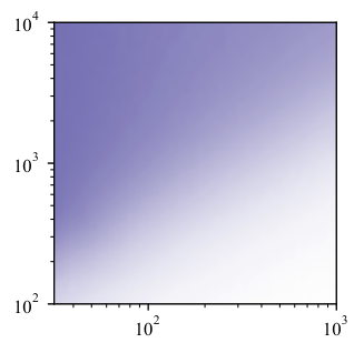
5.3 A phase transition in the fresh data loop
One might suspect that a complimentary perspective to the previous observation—that fresh new data mitigates the MAD generative process—is that synthetic data hurts a fresh data loop generative process. However, the truth appears to be more nuanced. What we find instead is that when we mix synthetic data trained on previous generations and fresh new data, there is a regime where modest amounts of synthetic data actually boost performance, but when synthetic data exceeds some critical threshold, the models suffer.
We make this observation precise through Gaussian simulations. Specifically, we consider the limit point of the fresh data loop from Equation 3. Using the value of this limit point, which we compute via Monte-Carlo simulation, we compare against an alternative model trained only on a collection of real data samples of size . We refer to as the effective sample size and compute its value given via
| (4) |
That is, captures the sample efficiency of the limit point of the fresh data loop. We evaluate the ratio in our experiments. When , the synthetic data effectively increases the number of real samples, which we consider to be admissible, while for , synthetic data effectively reduces the number of real samples.
We plot two perspectives of the results of this experiment in Figures 12 and 11, We discover several effects. First, we make some observations regarding sample sizes. We find that, indeed, for a given combination of and , there exists a phase transition in , such that if exceeds some admissible threshold, the effective sample size drops below the fresh data sample size. However, we do not find that the ratio of to is allowed to be constant; in fact, we find the opposite trend. For small values of , we find that large value of can be useful, but as grows larger, the phase transition threshold of seems to become constant.
Second, we make some observations regarding the effect of sampling bias parameter . We find that the value of the admissible threshold for depends strongly on the amount of sampling bias in the synthetic process. Perhaps surprisingly, more sampling bias (smaller ) actually reduces the number of synthetic samples that can be used without harming performance. Taking the limit as for unbiased sampling appears to ensure that the effective number of samples is always increased. Whether this limiting behavior extends to other generative models beyond the Gaussian modeling setting is unclear. As discussed in Section 2.3, it is unlikely that synthetic data is generated without sampling bias in practice, so we believe it is better to draw conclusions from the case.
More experiments for the fresh data loop can be found in Appendix G.


6 Discussion
In this paper we have sought to extrapolate what might happen in the near and distant future as generative models become ubiquitous and are used to train later generations of models in an autophagous (self-consuming) loop. Using analysis and experiments with state-of-the-art image generative models and standard image datasets, we have studied three families of autophagous loops and singled out the key rôle played by the models’ sampling bias. Some ramifications are clear: without enough fresh real data each generation, future generative models are doomed to Model Autophagy Disorder (MAD), meaning that either their quality (measured in terms of precision) or their diversity (measured in terms of recall) will progressively degrade and generative artifacts will be amplified. One doomsday scenario is that, if left uncontrolled for many generations, MAD could poison the data quality and diversity of the entire Internet. Short of this, it seems inevitable that as-to-now-unseen unintended consequences will arise from AI autophagy even in the near-term.
Practitioners who are deliberately using synthetic data for training because it is cheap and easy can take our conclusions as a warning and consider tempering their synthetic data habits, perhaps by joining an appropriate 12-step program. Those in truly data-scarce applications can interpret our results as a guide to how much scarce real data is necessary to avoid MADness in the future. For example, future practitioners who wish to train a comprehensive medical image generator using anonymous synthetic data from multiple institutions [30, 29] should now know that very deliberate care must be taken to ensure that: (i) all anonymous synthetic images are artifact-free and diverse (see the fully synthetic loop), and (ii) (ideally new) real data is present in the training as much as possible (see the fresh data loop and the synthetic augmentation loop).
Practitioners who have not been intending to use synthetic training but find it polluting their training data pool are harder to help. To maintain trustworthy datasets containing exclusively real data, the obvious recommendation is for the community to develop methods to identify synthetic data. These methods can then be used to filter training datasets to reject synthetic data or maintain a particular ratio of synthetic-to-real data. In this regard, there is early progress in the AI literature of new methods closely related to steganography [40] that can be employed for synthetic data identification. Since generative models do not necessarily add meta-data to generated images, another approach is to watermark synthetic data so that it can be identified and rejected when training. The reliability of watermarking of data generated by LLMs [75] and novel methods for watermarking LLMs [76], diffusion models [77, 78, 79, 80], andn GANs [81] are currently active areas of research. One reservation that we have about watermarking is that it deliberately introduces hidden artifacts in the synthetic data to make it detectable. These artifacts can possibly be amplified out of control by autophagy, turning watermarking from a useful to harmful. In fresh data loop we see that a large amount of synthetic data hurts performance, while a modest amount of synthetic data actually boosts performance. Watermarking can help out in this scenario to decrease the amount of synthetic data, and ideally put the model inside the good region (e.g., the blue area in Figure 11 and Figure 12), such that the negative aspects of watermarking are avoided. This opens up interesting avenues for research on autophagy-aware watermarking.
There are many possible extensions of the work reported here, including studying combinations of the three families of autophagous loops we have proposed. For example, one could analyze autophagous loops where the training data includes some synthetic data from previous generations’ models, some fixed real data, and some fresh real data. Our analysis has focused on the distance between the synthetic and reference data manifolds. An interesting research question is how this distance will manifest itself in lowered performance on AI tasks like classification (since precision can be closely related to classifier performance, the link is waiting to be made).
Finally, in this paper we have focused on imagery, but there is nothing about our conclusions that makes them image-specific. Generative models for any kind of data can be connected into autophagous loops and go MAD. One timely data type is the text produced by LLMs (some of which are already being trained on synthetic data from pre-existing models like ChatGPT) [57, 66, 67], where our results on precision and recall translate directly into the properties of the text produced after generations of autophagy. Similar conclusions have been reached in the experiments in the contemporaneous work of [53], but there is much work to do in this vein.
Acknowledgements
Thanks to Hamid Javadi, Blake Mason, and Shashank Sonkar for sharing their insights over the course of this project. This work was supported by NSF grants CCF-1911094, IIS-1838177, and IIS-1730574; ONR grants N00014-18-12571, N00014-20-1-2534, and MURI N00014-20-1-2787; AFOSR grant FA9550-22-1-0060; DOE grant DE-SC0020345; and a Vannevar Bush Faculty Fellowship, ONR grant N00014-18-1-2047.
Appendix A Proof of synthetic Gaussian martingale variance collapse
We now prove that for the process described in Equation 1, .
Proof.
First write for . Then consider the process , which is a lower bounded submartingale:
| (5) |
where . By Doob’s martingale convergence theorem [72, Ch. 11], there exists a random variable such that , and we now show that we must have . Without loss of generality, we can assume that is diagonal, in which case it becomes clear that is a generalized random variable, being a linear combination of independent random variables with degrees of freedom, mixed with weights . Therefore, we can write , where is a generalized random variable with the same degrees of freedom but with mixing weights , and . This implies that at least one mixing weight is greater than for each , which means that for any , there exists such that . Now consider the case . Since infinitely often with probability one, the only that can satisfy is . For general , is simply the product of the process for and the sequence , and so the product must also converge to zero almost surely. Finally, since , we also must have , where convergence is defined with any matrix norm. ∎
Appendix B Additional experiments for the fully synthetic loop
Here we present additional experiments for the fully synthetic loop.
B.1 WGAN-GPs in an unbiased fully synthetic loop
In this experiment we trained Wasserstein GANs (with gradient penalty) [60] on the MNIST dataset in a fully synthetic loop for 100 generations. As shown in Figure 13, the FID monotonically increases, while quality (precision) and diversity (recall) monotonically decrease.
B.2 GMMs in an unbiased fully synthetic loop
We also trained 2D GMMs in an unbiased fully synthetic loop using the same 25-mode distribution as [82]. In Figure 14 we see that the fully synthetic loop gradually reduces the number of modes covered by the synthetic distribution. Various metrics could measure this loss in diversity, so in Figure 15 we explore how well each metric reflects the dynamics of the fully synthetic loop, finding that recall is best-equipped to measure diversity in multimodal datasets.
B.3 Additional MNIST DDPM fully synthetic loop results
In Figure 6 we showcased the results of training MNIST DDPMs in a fully synthetic loop with various sampling bias factors . In Figure 16 we have the results (FID, precision, and recall) more generations and different sampling biases .
B.4 Normalizing flow fully synthetic loop
We implemented the fully synthetic loop using normalizing flows [83, 84] for generative modeling of the two-dimensional Rosenbrock reference distribution [85] in order to visualize the outcome of this particular scenario in a controlled setting. Normalizing flows are unique in that they enable exact evaluation of the likelihood of the estimated distribution due to their invertibility [83]. This leads to a relatively straightforward training procedure compared to GANs, which often require careful balancing between the generator and discriminator networks to avoid mode collapse [86]. Therefore, by using a low-dimensional reference distribution, this setup allows us to demonstrate the fully synthetic loop while eliminating potential training imperfections.
According to the fully synthetic loop setup, we start with a training dataset of samples from the 2D Rosenbrock distribution with the density function [85], which is plotted on the left-hand side of Figure 17. The subsequent generations of normalizing flow models are trained using synthetic data generated by the previous pre-trained normalizing flow for generations, both with and without sampling bias. We employ the GLOW normalizing flow architecture [84] with eight coupling layers [84] and a hidden dimension of . The training is carried out for epochs with a batch size of for each generation, ensuring convergence as determined by monitoring the model’s likelihood over a validation set. Figure 17 summarizes the results of this fully synthetic loop setup. To incorporate sampling bias, we sample from from the latent space of the model, where . As shown, regardless of the presence of sampling bias, the resulting distribution after generations loses the tails of the reference distribution, indicating a loss of diversity. This phenomenon becomes more pronounced when sampling bias is present ().
Appendix C FFHQ fully synthetic loop images with
We show additional randomly chosen synthetic samples produced by the same StyleGAN FFHQ unbiased fully synthetic loop as in Figure 1 and Figure 4.


Appendix D FFHQ fully synthetic loop images with
As in Appendix C, here we show synthetic FFHQ images produced by a StyleGAN architecture in a fully synthetic loop with biased sampling (, Figure 6) that slows the proliferation of artifacts, but at the cost of severely decreased diversity.


Appendix E MNIST fully synthetic loop images
Here we show randomly chosen samples from each generation of an MNIST DDPM in a fully synthetic loop for different sampling biases (as discussed in Figure 4 and Figure 6).
Gen. 1 2 3 4 5 6 7 8 9 10 11 12 13 14 15 16 17 18 19 20

Gen. 1 2 3 4 5 6 7 8 9 10 11 12 13 14 15 16 17 18 19 20

Appendix F FFHQ synthetic augmentation loop images with


Appendix G Additional results for the fresh data loop
Here we provide three additional Gaussian experiments investigating the convergence of the fresh data loop.
Experiment 1: In Section 5.1 we assumed that we only sample from the previous generation for creating the synthetic dataset . In this experiment we sample randomly from previous models . Here , , and . In Figure 30 we see how varies with respect to . Increasing the memory in sampling from previous generations can boost performance, however the rate of improvement becomes slower as increases.
Experiment 2: Here we assume that we are sampling from an environment where percent of data is real, and the rest is synthetic data from the previous generation with sampling bias . We change the total number of data in the dataset , with and . We show the Wasserstein distance for different and in Figure 31.
Let us first examine the dynamics of the Gaussian fresh data loop without sampling bias (). We observe in Figure 31 (left) that the Wasserstein distance (WD) decreases with respect to dataset size . However, the presence of synthetic data () decreases the rate at which the WD decreases, and increases the overall WD each generation in the fresh data loop. This means that with presence of synthetic data in the Internet, the progress of generative models will become slower
In the presence of sampling bias (, Figure 31 right), we see that even for close values of to 1, the Wasserstein distance follows a sub-linear trend, meaning that eventually the rate of progress in generative models will effectively stop, no matter how much (realistically) the total dataset size is increased.
References
- Karras et al. [2019] Tero Karras, Samuli Laine, and Timo Aila. A style-based generator architecture for generative adversarial networks. In CVPR, 2019.
- Rombach et al. [2022] Robin Rombach, Andreas Blattmann, Dominik Lorenz, Patrick Esser, and Björn Ommer. High-resolution image synthesis with latent diffusion models. In CVPR, 2022.
- Ramesh et al. [2022] Aditya Ramesh, Prafulla Dhariwal, Alex Nichol, Casey Chu, and Mark Chen. Hierarchical text-conditional image generation with clip latents. arXiv preprint arXiv:2204.06125, 2022.
- Borsos et al. [2022] Zalán Borsos, Raphaël Marinier, Damien Vincent, Eugene Kharitonov, Olivier Pietquin, Matt Sharifi, Olivier Teboul, David Grangier, Marco Tagliasacchi, and Neil Zeghidour. AudioLM: a language modeling approach to audio generation. arXiv preprint arXiv:2209.03143, 2022.
- Agostinelli et al. [2023] Andrea Agostinelli, Timo I. Denk, Zalán Borsos, Jesse Engel, Mauro Verzetti, Antoine Caillon, Qingqing Huang, Aren Jansen, Adam Roberts, Marco Tagliasacchi, Matt Sharifi, Neil Zeghidour, and Christian Frank. MusicLM: Generating music from text. arXiv preprint arXiv:2301.11325, 2023.
- ElevenLabs [2022] ElevenLabs. First long-form speech synthesis platform for publishers and creators. 2022. URL https://blog.elevenlabs.io/long-form-speech-synthesis-for-publishers-and-creators/.
- OpenAI [2023] OpenAI. GPT-4 technical report. arXiv preprint arXiv:2303.08774, 2023.
- Touvron et al. [2023] Hugo Touvron, Thibaut Lavril, Gautier Izacard, Xavier Martinet, Marie-Anne Lachaux, Timothée Lacroix, Baptiste Rozière, Naman Goyal, Eric Hambro, Faisal Azhar, Aurelien Rodriguez, Armand Joulin, Edouard Grave, and Guillaume Lample. LLaMA: Open and efficient foundation language models. arXiv preprint arXiv:2302.13971, 2023.
- Dai et al. [2023] Haixing Dai, Zhengliang Liu, Wenxiong Liao, Xiaoke Huang, Yihan Cao, Zihao Wu, Lin Zhao, Shaochen Xu, Wei Liu, Ninghao Liu, Sheng Li, Dajiang Zhu, Hongmin Cai, Lichao Sun, Quanzheng Li, Dinggang Shen, Tianming Liu, and Xiang Li. AugGPT: Leveraging ChatGPT for text data augmentation. arXiv preprint arXiv:2302.13007, 2023.
- Poole et al. [2023] Ben Poole, Ajay Jain, Jonathan T. Barron, and Ben Mildenhall. Dreamfusion: Text-to-3d using 2d diffusion. In ICLR, 2023.
- Villegas et al. [2023] Ruben Villegas, Mohammad Babaeizadeh, Pieter-Jan Kindermans, Hernan Moraldo, Han Zhang, Mohammad Taghi Saffar, Santiago Castro, Julius Kunze, and Dumitru Erhan. Phenaki: Variable length video generation from open domain textual descriptions. In ICLR, 2023.
- Vignac et al. [2023] Clement Vignac, Igor Krawczuk, Antoine Siraudin, Bohan Wang, Volkan Cevher, and Pascal Frossard. DiGress: Discrete denoising diffusion for graph generation. In ICLR, 2023.
- Kotelnikov et al. [2022] Akim Kotelnikov, Dmitry Baranchuk, Ivan Rubachev, and Artem Babenko. TabDDPM: Modelling tabular data with diffusion models. arXiv preprint arXiv:2209.15421, 2022.
- Becker et al. [2023] Brett A Becker, Paul Denny, James Finnie-Ansley, Andrew Luxton-Reilly, James Prather, and Eddie Antonio Santos. Programming is hard-or at least it used to be: Educational opportunities and challenges of AI code generation. In ACM Technical Symposium on Computer Science Education V.1, 2023.
- Cantor [2023] Matthew Cantor. Nearly 50 news websites are ‘AI-generated’, a study says. Would I be able to tell? The Guardian, May 2023.
- Gozalo-Brizuela and Garrido-Merchan [2023] Roberto Gozalo-Brizuela and Eduardo C. Garrido-Merchan. ChatGPT is not all you need. a state of the art review of large generative ai models. arXiv preprint arXiv:2301.04655, 2023.
- Schuhmann et al. [2022] Christoph Schuhmann et al. LAION-5B: An open large-scale dataset for training next generation image-text models. In NeurIPS Datasets and Benchmarks Track, 2022.
- Gault [2023] Matthew Gault. AI spam is already flooding the internet and it has an obvious tell. VICE, April 2023.
- Christian [2023] Jon Christian. CNET secretly used AI on articles that didn’t disclose that fact, staff say. Futurusm, January 2023.
- He et al. [2023] Ruifei He, Shuyang Sun, Xin Yu, Chuhui Xue, Wenqing Zhang, Philip Torr, Song Bai, and Xiaojuan Qi. Is synthetic data from generative models ready for image recognition? In ICLR, 2023.
- Shipard et al. [2023] Jordan Shipard, Arnold Wiliem, Kien Nguyen Thanh, Wei Xiang, and Clinton Fookes. Diversity is definitely needed: Improving model-agnostic zero-shot classification via stable diffusion. arXiv preprint arXiv:2302.03298, 2023.
- Bansal and Grover [2023] Hritik Bansal and Aditya Grover. Leaving reality to imagination: Robust classification via generated datasets. arXiv preprint arXiv:2302.02503, 2023.
- Lin et al. [2023] Shaobo Lin, Kun Wang, Xingyu Zeng, and Rui Zhao. Explore the power of synthetic data on few-shot object detection. arXiv preprint arXiv:2303.13221, 2023.
- Xu et al. [2023] Canwen Xu, Daya Guo, Nan Duan, and Julian McAuley. Baize: An open-source chat model with parameter-efficient tuning on self-chat data. arXiv preprint arXiv:2304.01196, 2023.
- Azizi et al. [2023] Shekoofeh Azizi, Simon Kornblith, Chitwan Saharia, Mohammad Norouzi, and David J Fleet. Synthetic data from diffusion models improves imagenet classification. arXiv preprint arXiv:2304.08466, 2023.
- Burg et al. [2023] Max F Burg, Florian Wenzel, Dominik Zietlow, Max Horn, Osama Makansi, Francesco Locatello, and Chris Russell. A data augmentation perspective on diffusion models and retrieval. arXiv preprint arXiv:2304.10253, 2023.
- Luzi et al. [2022] Lorenzo Luzi, Ali Siahkoohi, Paul M Mayer, Josue Casco-Rodriguez, and Richard Baraniuk. Boomerang: Local sampling on image manifolds using diffusion models. arXiv preprint arXiv:2210.12100, 2022.
- Klemp et al. [2023] Marvin Klemp, Kevin Rösch, Royden Wagner, Jannik Quehl, and Martin Lauer. LDFA: Latent diffusion face anonymization for self-driving applications. arXiv preprint arXiv:2302.08931, 2023.
- Packhäuser et al. [2022] Kai Packhäuser, Lukas Folle, Florian Thamm, and Andreas Maier. Generation of anonymous chest radiographs using latent diffusion models for training thoracic abnormality classification systems. arXiv preprint arXiv:2211.01323, 2022.
- DuMont Schütte et al. [2021] August DuMont Schütte, Jürgen Hetzel, Sergios Gatidis, Tobias Hepp, Benedikt Dietz, Stefan Bauer, and Patrick Schwab. Overcoming barriers to data sharing with medical image generation: a comprehensive evaluation. NPJ Digital Medicine, 2021.
- big [2023] The bigger-is-better approach to AI is running out of road. The Economist, June 2023.
- lar [2023] Large, creative AI models will transform lives and labour markets. The Economist, April 2023.
- Villalobos et al. [2022] Pablo Villalobos, Jaime Sevilla, Lennart Heim, Tamay Besiroglu, Marius Hobbhahn, and Anson Ho. Will we run out of data? an analysis of the limits of scaling datasets in machine learning. arXiv preprint arXiv:2211.04325, 2022.
- Veselovsky et al. [2023] Veniamin Veselovsky, Manoel Horta Ribeiro, and Robert West. Artificial artificial artificial intelligence: Crowd workers widely use large language models for text production tasks. arXiv preprint arXiv:2306.07899, 2023.
- Elgammal et al. [2017] Ahmed Elgammal, Bingchen Liu, Mohamed Elhoseiny, and Marian Mazzone. CAN: Creative adversarial networks, generating "art" by learning about styles and deviating from style norms. arXiv preprint arXiv:1706.07068, 2017.
- Isola et al. [2017] Phillip Isola, Jun-Yan Zhu, Tinghui Zhou, and Alexei A Efros. Image-to-image translation with conditional adversarial networks. In CVPR, 2017.
- Ramesh et al. [2021] Aditya Ramesh, Mikhail Pavlov, Gabriel Goh, Scott Gray, Chelsea Voss, Alec Radford, Mark Chen, and Ilya Sutskever. Zero-shot text-to-image generation. In ICML, 2021.
- Brock et al. [2019] Andrew Brock, Jeff Donahue, and Karen Simonyan. Large scale GAN training for high fidelity natural image synthesis. In ICLR, 2019.
- Kynkäänniemi et al. [2019] Tuomas Kynkäänniemi, Tero Karras, Samuli Laine, Jaakko Lehtinen, and Timo Aila. Improved precision and recall metric for assessing generative models. NeurIPS, 2019.
- Guarnera et al. [2020] Luca Guarnera, Oliver Giudice, and Sebastiano Battiato. Deepfake detection by analyzing convolutional traces. In CVPR workshops, 2020.
- Karras et al. [2021] Tero Karras, Miika Aittala, Samuli Laine, Erik Härkönen, Janne Hellsten, Jaakko Lehtinen, and Timo Aila. Alias-free generative adversarial networks. In NeurIPS, 2021.
- Ho and Salimans [2021] Jonathan Ho and Tim Salimans. Classifier-free diffusion guidance. In NeurIPS 2021 Workshop on Deep Generative Models and Downstream Applications, 2021.
- Stroud [2011] Natalie Jomini Stroud. Niche News: The Politics of News Choice. Oxford University Press, 2011.
- Dylko et al. [2017] Ivan Dylko, Igor Dolgov, William Hoffman, Nicholas Eckhart, Maria Molina, and Omar Aaziz. The dark side of technology: An experimental investigation of the influence of customizability technology on online political selective exposure. Computers in Human Behavior, 2017.
- Beam [2014] Michael A Beam. Automating the news: How personalized news recommender system design choices impact news reception. Communication Research, 2014.
- Bakshy et al. [2015] Eytan Bakshy, Solomon Messing, and Lada A Adamic. Exposure to ideologically diverse news and opinion on Facebook. Science, 2015.
- O’Callaghan et al. [2015] Derek O’Callaghan, Derek Greene, Maura Conway, Joe Carthy, and Pádraig Cunningham. Down the (white) rabbit hole: The extreme right and online recommender systems. Social Science Computer Review, 2015.
- Brown et al. [2022] Megan A Brown, James Bisbee, Angela Lai, Richard Bonneau, Jonathan Nagler, and Joshua A Tucker. Echo chambers, rabbit holes, and algorithmic bias: How youtube recommends content to real users. SSRN 4114905, 2022.
- Möller et al. [2018] Judith Möller, Damian Trilling, Natali Helberger, and Bram van Es. Do not blame it on the algorithm: an empirical assessment of multiple recommender systems and their impact on content diversity. Information, Communication & Society, 2018.
- Nathanson et al. [1997] Neal Nathanson, John Wilesmith, and Christian Griot. Bovine Spongiform Encephalopathy (BSE): Causes and Consequences of a Common Source Epidemic. American Journal of Epidemiology, 145(11):959–969, 06 1997. ISSN 0002-9262.
- Casco-Rodriguez [2023] Josue Casco-Rodriguez. Toward understanding the impact of generative AI on future generative AI. Electrical & Computer Engineering Technical Report No. 2023–04–79 (ELEC599), Rice University, 9 April 2023.
- Casco-Rodriguez et al. [2023] Josue Casco-Rodriguez, Lorenzo Luzi, Sina Alemohammad, Shashank Sonkar, Ahmed Imtiaz Humayun, Ali Siahkoohi, and Richard Baraniuk. Toward understanding the impact of generative AI on future generative AI. In Interface Rice. Rice University Neuroengineering Initiative, 18 May 2023.
- Shumailov et al. [2023] Ilia Shumailov, Zakhar Shumaylov, Yiren Zhao, Yarin Gal, Nicolas Papernot, and Ross Anderson. The curse of recursion: Training on generated data makes models forget. arXiv preprint arXiv:2305.17493, 2023.
- Martínez et al. [2023a] Gonzalo Martínez, Lauren Watson, Pedro Reviriego, José Alberto Hernández, Marc Juarez, and Rik Sarkar. Towards understanding the interplay of generative artificial intelligence and the Internet. arXiv preprint arXiv:2306.06130, 2023a.
- Martínez et al. [2023b] Gonzalo Martínez, Lauren Watson, Pedro Reviriego, José Alberto Hernández, Marc Juarez, and Rik Sarkar. Combining generative artificial intelligence (ai) and the Internet: Heading towards evolution or degradation? arXiv preprint arXiv:2303.01255, 2023b.
- followfox.ai [2023] followfox.ai. The power of synthetic data: Infinite loop to improve fine-tuning results with stable diffusion models. February 2023. URL https://followfoxai.substack.com/p/the-power-of-synthetic-data-infinite.
- Huang et al. [2022] Jiaxin Huang, Shixiang Shane Gu, Le Hou, Yuexin Wu, Xuezhi Wang, Hongkun Yu, and Jiawei Han. Large language models can self-improve. arXiv preprint arXiv:2210.11610, 2022.
- Karras et al. [2020] Tero Karras, Samuli Laine, Miika Aittala, Janne Hellsten, Jaakko Lehtinen, and Timo Aila. Analyzing and improving the image quality of StyleGAN. In CVPR, 2020.
- Ho et al. [2020] Jonathan Ho, Ajay Jain, and Pieter Abbeel. Denoising diffusion probabilistic models. In NeurIPS, 2020.
- Gulrajani et al. [2017a] Ishaan Gulrajani, Faruk Ahmed, Martin Arjovsky, Vincent Dumoulin, and Aaron C Courville. Improved training of Wasserstein GANs. NeurIPS, 2017a.
- Kobyzev et al. [2020] Ivan Kobyzev, Simon JD Prince, and Marcus A Brubaker. Normalizing flows: An introduction and review of current methods. IEEE Transactions on Pattern Analysis and Machine Intelligence, (11), 2020.
- Deng [2012] Li Deng. The MNIST database of handwritten digit images for machine learning research [best of the web]. IEEE Signal Processing Magazine, (6), 2012.
- Kass and Vos [1997] Robert E Kass and Paul W Vos. Geometrical Foundations of Asymptotic Inference. John Wiley & Sons, 1997.
- Pinaya et al. [2022] Walter H. L. Pinaya, Petru-Daniel Tudosiu, Jessica Dafflon, Pedro F. Da Costa, Virginia Fernandez, Parashkev Nachev, Sebastien Ourselin, and M. Jorge Cardoso. Brain imaging generation with latent diffusion models. In Deep Generative Models. Springer Nature, 2022.
- Deng et al. [2022] Chengyuan Deng, Shihang Feng, Hanchen Wang, Xitong Zhang, Peng Jin, Yinan Feng, Qili Zeng, Yinpeng Chen, and Youzuo Lin. OpenFWI: Large-scale multi-structural benchmark datasets for full waveform inversion. In NeurIPS, 2022.
- Wang et al. [2022] Yizhong Wang, Yeganeh Kordi, Swaroop Mishra, Alisa Liu, Noah A Smith, Daniel Khashabi, and Hannaneh Hajishirzi. Self-instruct: Aligning language model with self generated instructions. arXiv preprint arXiv:2212.10560, 2022.
- Taori et al. [2023] Rohan Taori, Ishaan Gulrajani, Tianyi Zhang, Yann Dubois, Xuechen Li, Carlos Guestrin, Percy Liang, and Tatsunori B Hashimoto. Alpaca: A strong, replicable instruction-following model. Stanford Center for Research on Foundation Models., (6), 2023.
- Humayun et al. [2022] Ahmed Imtiaz Humayun, Randall Balestriero, and Richard Baraniuk. Polarity sampling: Quality and diversity control of pre-trained generative networks via singular values. In CVPR, 2022.
- Kantorovich [1960] Leonid V Kantorovich. Mathematical Methods of Organizing and Planning Production. Management science, (4), 1960.
- Heusel et al. [2017] Martin Heusel, Hubert Ramsauer, Thomas Unterthiner, Bernhard Nessler, and Sepp Hochreiter. GANs trained by a two time-scale update rule converge to a local Nash equilibrium. In NeurIPS, 2017.
- Song et al. [2021] Jiaming Song, Chenlin Meng, and Stefano Ermon. Denoising diffusion implicit models. In International Conference on Learning Representations, 2021.
- Williams [1991] David Williams. Probability With Martingales. Cambridge University Press, 1991.
- Lecun et al. [1998] Y. Lecun, L. Bottou, Y. Bengio, and P. Haffner. Gradient-based learning applied to document recognition. Proceedings of the IEEE, 1998.
- Van der Maaten and Hinton [2008] Laurens Van der Maaten and Geoffrey Hinton. Visualizing data using t-SNE. JMLR, 2008.
- Kirchenbauer et al. [2023a] John Kirchenbauer, Jonas Geiping, Yuxin Wen, Manli Shu, Khalid Saifullah, Kezhi Kong, Kasun Fernando, Aniruddha Saha, Micah Goldblum, and Tom Goldstein. On the reliability of watermarks for large language models. arXiv preprint arXiv:2306.04634, 2023a.
- Kirchenbauer et al. [2023b] John Kirchenbauer, Jonas Geiping, Yuxin Wen, Jonathan Katz, Ian Miers, and Tom Goldstein. A watermark for large language models. arXiv preprint arXiv:2301.10226, 2023b.
- Zhao et al. [2023] Yunqing Zhao, Tianyu Pang, Chao Du, Xiao Yang, Ngai-Man Cheung, and Min Lin. A recipe for watermarking diffusion models. arXiv preprint arXiv:2303.10137, 2023.
- Peng et al. [2023] Sen Peng, Yufei Chen, Cong Wang, and Xiaohua Jia. Protecting the intellectual property of diffusion models by the watermark diffusion process. arXiv preprint arXiv:2306.03436, 2023.
- Wen et al. [2023] Yuxin Wen, John Kirchenbauer, Jonas Geiping, and Tom Goldstein. Tree-ring watermarks: Fingerprints for diffusion images that are invisible and robust. arXiv preprint arXiv:2305.20030, 2023.
- Fernandez et al. [2023] Pierre Fernandez, Guillaume Couairon, Hervé Jégou, Matthijs Douze, and Teddy Furon. The stable signature: Rooting watermarks in latent diffusion models. arXiv preprint arXiv:2303.15435, 2023.
- Fei et al. [2022] Jianwei Fei, Zhihua Xia, Benedetta Tondi, and Mauro Barni. Supervised GAN watermarking for intellectual property protection. In Workshop on Information Forensics and Security (WIFS), 2022.
- Che et al. [2020] Tong Che, Ruixiang Zhang, Jascha Sohl-Dickstein, Hugo Larochelle, Liam Paull, Yuan Cao, and Yoshua Bengio. Your GAN is secretly an energy-based model and you should use discriminator driven latent sampling. In NeurIPS, 2020.
- Dinh et al. [2016] Laurent Dinh, Jascha Sohl-Dickstein, and Samy Bengio. Density estimation using Real NVP. In International Conference on Learning Representations, ICLR, 2016. URL http://arxiv.org/abs/1605.08803.
- Kingma and Dhariwal [2018] Durk P Kingma and Prafulla Dhariwal. Glow: Generative Flow with Invertible 1x1 Convolutions. In Advances in Neural Information Processing Systems, 2018.
- Pagani et al. [2022] Filippo Pagani, Martin Wiegand, and Saralees Nadarajah. An n-dimensional Rosenbrock distribution for Markov chain Monte Carlo testing. Scandinavian Journal of Statistics, (2), 2022.
- Gulrajani et al. [2017b] Ishaan Gulrajani, Faruk Ahmed, Martin Arjovsky, Vincent Dumoulin, and Aaron C Courville. Improved training of Wasserstein GANs. In Advances in Neural Information Processing Systems, 2017b.