Precise characterization of nanometer-scale systems using interferometric scattering microscopy and Bayesian analysisJournal: opticajournal
Abstract
Interferometric scattering microscopy (iSCAT) can image the dynamics of nanometer-scale systems. The typical approach to analyzing interferometric images involves intensive processing, which discards data and limits the precision of measurements. We demonstrate an alternative approach: modeling the interferometric point spread function (iPSF) and fitting this model to data within a Bayesian framework. This approach yields best-fit parameters, including the particle’s three-dimensional position and polarizability, as well as uncertainties and correlations between these parameters. Building on recent work, we develop a model that is parameterized for rapid fitting. The model is designed to work with Hamiltonian Monte Carlo techniques that leverage automatic differentiation. We validate this approach by fitting the model to interferometric images of colloidal nanoparticles. We apply the method to track a diffusing particle in three dimensions, to directly infer the diffusion coefficient of a nanoparticle without calculating a mean-square displacement, and to quantify the ejection of DNA from an individual lambda phage virus, demonstrating that the approach can be used to infer both static and dynamic properties of nanoscale systems.
1 Introduction
Interferometric scattering microscopy (iSCAT) takes advantage of the interference between elastically scattered light and a weak reference beam to detect small particles such as biomolecules and nanospheres [1]. The principal advantage of this technique over fluorescent-based imaging is that it is label-free. It therefore entails little risk of photobleaching or heating, allowing samples to be imaged at high frame-rates over long times [2, 3, 4]. Furthermore, an interferometric image encodes information about the size and three-dimensional (3D) position of the particle that produced it, making iSCAT useful for sensitive, nanoscale measurements, such as characterizing the mass distribution of molecular complexes [5], the polymerization of protein filaments [6], the rates of DNA ejection from bacteriophages [7], and the kinetics of viral self-assembly [8].

These measurements rely on algorithms that infer sizes and positions of nanoparticles or nanoassemblies. The most frequently used algorithms extract this information primarily from the central spot of the iSCAT image. For example, quantifying the interferometric contrast of the central spot of an iSCAT image of a biomolecular assembly yields a measurement of its mass [6]. Also, fitting a Gaussian function to the intensity profile of the center of an iSCAT image of a nanoparticle yields a measurement of its two-dimensional (2D) position to nanometer-scale precision [9]. However, such algorithms discard information such as the interference fringes outside the central spot, which contain additional information about size and 3D position. Furthermore, these methods cannot easily make use of prior information – for example, the expected particle size – and do not easily account for correlations – for example, between size and position – making it difficult to quantify uncertainties on the measurements.
An alternative method is to model both the scattering and interference and fit that model to the data. This forward modeling approach has been used to analyze interferometric images from an in-line holographic microscope, which has a different configuration than the iSCAT microscope but operates on similar principles. For example, fitting a forward model of Lorenz-Mie scattering, interference, and propagation to an in-line hologram enables precise characterization and 3D tracking of microscopic particles [10], with quantified uncertainties [11, 12, 13, 14]. Recently, the forward modeling approach has been extended to iSCAT. Mahmoodabadi and coworkers [15] developed a forward model of the interferometric point spread function (iPSF), including the effects of an objective lens, and fit this model to iSCAT data to extract 3D trajectories of gold nanoparticles. Modeling interferometric images as point-spread functions is a reasonable approximation here because the particles are much smaller than the wavelength of light. More recently, Kashkanova and coworkers [16] applied a Lorenz-Mie scattering solution, applicable to larger particles, to quantify the intensities of processed iSCAT images, and He and coworkers [17] developed a general approach based on numerical electromagnetic simulations.
Our aim is to develop a forward modeling approach that yields precise measurements of specimen size, mass, and 3D position, makes use of information in both the central spot and surrounding fringes, readily incorporates prior information, and accurately quantifies uncertainties. To this end, we use a Bayesian parameter-estimation framework. We infer the posterior probability density (or “posterior”) of the parameters in the forward model given the data and prior information, which is specified as prior probability distributions (or “priors”) on the parameters. In contrast to fits obtained by non-linear optimization techniques [18, 19], the full posterior obtained in a Bayesian approach describes more than just the best-fit values; it can also be used to infer the correlations between parameters and the marginalized uncertainty of each parameter, which accounts for these correlations.
To implement this approach, we must develop a computationally simple forward model that can be used with Markov chain Monte Carlo (MCMC) sampling methods, the typical approach to calculating the posterior in a Bayesian framework [20, 11, 21]. Sampling the posterior with MCMC methods requires thousands of model evaluations. We must therefore make physical approximations to limit the computational complexity of the model, so that sampling takes a reasonable time. Furthermore, the model must be expressed so as to allow efficient sampling in a multi-dimensional parameter space. The most efficient MCMC methods are based on Hamiltonian Monte Carlo (HMC) algorithms [22], which rely on automatic differentiation to calculate gradients [23]. To leverage these algorithms, we must express our model using a modern, computational graph library.
To enable HMC-based analysis of iSCAT data, we focus on the Rayleigh scattering regime, applicable to particles much smaller than the incident wavelength. This approximation allows us to use the iPSF to model the iSCAT image, as previously shown by Mahmoodabadi and coworkers [15]. Here, we re-parameterize the forward model of the iPSF so that it can be used with a computational graph library and HMC sampler, both implemented in the Python package PyMC [24]. Furthermore, we use a much simpler model for the optical train of the microscope, one that ignores effects of the objective other than magnification. This choice reduces the computational cost of each model evaluation. As we show, our approach can efficiently estimate parameters from iSCAT data along with their correlations and uncertainties, even when the posterior is multi-modal. We demonstrate several applications of this approach, including tracking diffusing nanoparticles in 3D, directly inferring diffusion coefficients from position data, and characterizing the ejection of DNA from a lambda phage, a virus that infects E. coli bacteria.
2 Model of the iPSF
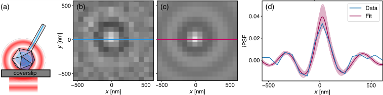
In iSCAT, coherent light illuminates a sample through an objective lens. The light is scattered by the particles in the sample, and a portion of the incident beam is reflected by the interface of the coverslip (Fig. 1a, b). The scattered field () and reflected field () return through the objective and interfere to form an image. For a single subwavelength particle, the resulting interferometric image is a set of concentric bright and dark rings (Fig. 1c) that can be modeled with the iPSF.
2.1 The simplified model
For simplicity, we assume that the interference pattern is translated one-to-one from the focal plane of the objective lens onto the camera, an assumption widely used in analysis of data from in-line holographic microscopy [10, 14]. This approximation neglects any aberrations induced by the coverslip or optical train and assumes the particle is above the focal plane. Nonetheless, analysis of in-line holograms shows that the approximation is reasonable if the particle is at least a few micrometers above the focal plane and the objective has a high numerical aperture [12]. For our purposes, this approximation enables a more efficient parameterization that allows us to avoid computationally expensive numerical integrations or special-function evaluations.
With this approximation, the intensity profile of the interference pattern is
| (1) | ||||
Here, the coordinate system has the -axis aligned with the optical axis, where is the top of the coverslip, and is the position of the focal plane. is the phase difference between and (we have omitted the arguments for brevity). We normalize by and subtract the contribution of the reference beam to obtain the iPSF as
| (2) |
We neglect the term because for weakly scattering systems.
To evaluate this expression at the focal plane, we first consider a reference beam aligned with the optical axis with a constant intensity profile. Though the beam never reaches the focal plane physically, we can treat it as if it originates at the focal plane by including an additional phase shift of , where is the refractive index of the medium and is the vacuum wavevector. Fresnel reflection from the refractive-index mismatch at the coverslip-sample interface induces an additional phase shift . We thus find that at the focal plane
| (3) |
In the Rayleigh approximation, the scattered field from a sphere at a distance in the far-field limit is
| (4) |
where is the incident light, is the particle polarizability relative to the medium, is the incident wavelength, and is the scattering angle [25]. The polarizability is proportional to the volume of the particle. For a spherical particle,
| (5) |
where is the particle radius and is its refractive index. Because can be complex, it can lead to an additional phase difference between the incident and scattered wave. The scattered field at the focal plane can be evaluated from (4) with , the distance between the position on the focal plane and the particle position . The scattering angle is then .
Finally, by accounting for the additional phase factor of in the incident beam, corresponding to the optical path length from the coverslip to the particle, we obtain the following expressions for the terms in (2):
| (6) | ||||

2.2 Parameterization
Several parameters in (6) have equivalent effects on the iPSF and cannot be independently inferred. We reparameterize to avoid such degeneracies and minimize the correlation between parameters, which is computationally beneficial for MCMC. We define the following parameters: the height of the particle with respect to the focal plane , a lumped amplitude
| (7) |
and a lumped phase
| (8) |
Because or can be precisely measured, we do not include them as parameters. With the new parameterization, (2) can be expressed in terms of the following quantities:
| (9) | ||||
with . We substitute these quantities into (2) and eliminate to arrive at
| (10) |
We find good agreement between this model and the more complex model developed by Mahmoodabadi and coworkers [15] (Fig. 2; compare with Fig. 3b of Ref. 15, below the dashed line).
2.3 Beam misalignment
In many iSCAT experiments, the reference beam is purposely misaligned with the optical axis to avoid unwanted reflections. The deformation of the interference pattern caused by misalignment would introduce a systematic error in the inferred parameters if it were not modeled.
We model the misalignment by considering the spatially varying phase shift at the focal plane, which we parameterize by two angles: , the angle between the beam and the optical axis (Fig. 3a), and , the rotation of the beam about the optical axis. We first project each position on the focal plane to a distance along the unit vector :
| (11) |
The spatially varying phase shift is related to the perpendicular distance from the equiphase line (Fig. 3a) as
| (12) |
There is also a phase shift of the beam incident on the particle at , such that the relative phase shift is
| (13) |
Other than this phase shift, we assume that there is no additional effect from the beam misalignment on the scattering angle, an approximation that is valid if the detector subtends a sufficiently small angle, as is the case here.

By including this phase shift in our model, we can calculate the iPSF for any values of and , as shown in Fig. 3b. Because these parameters should not vary within a single experiment, they can either be inferred or directly measured and then set as constant. Through inference, we find in our experiments that and . The degree of asymmetry in the iPSF depends on the degree of misalignment of the beam; when the beam is only slightly misaligned, this effect becomes negligible.
2.4 Beam Gaussianity
Although a typical incident beam is spatially filtered, resulting in a Gaussian profile, it is reasonable to approximate the beam profile as uniform when the iPSF is much smaller than the beam width. With strongly scattering particles, however, the extent of the iPSF can be comparable to the beam size. This is the case for the larger polystyrene particles (100 nm) that we examine in some of our experiments, though not for the lambda phage particles. Thus, we correct for beam Gaussianity for analysis of polystyrene particles but approximate the beam as uniform for analysis of the smaller phage (see Supplemental Document).
3 Bayesian inference for iSCAT
To estimate the free parameters of our model along with their uncertainties, we first process the raw iSCAT images according to the scheme in Ref. 26, then use a Bayesian MCMC method to fit the model to the processed data. The processing algorithm estimates the background from the image by filtering, subtracts off the estimated background, and finally divides the image by the estimated background. We crop the image to the region with visible fringes to avoid fitting to areas where the signal-to-noise ratio is low. We model the noise as independent and Gaussian for each pixel with constant standard deviation , which we include as an additional free parameter in the model to better estimate the noise level. When we estimate other parameters, we marginalize over the noise parameter, incorporating its uncertainty into the uncertainties of the parameters of interest.

A Bayesian framework requires explicit choices of prior probabilities for each free parameter. We choose normal distributions for parameters that can be positive or negative, such as position, and gamma distributions for parameters that must be positive, such as scattering amplitude. For the phase factor , we use a uniform distribution from to . For the misalignment angles, we use truncated normal distributions to constrain the angles to the appropriate quadrant. We find that fitting converges with relatively uninformative priors on all parameters except for the horizontal position , which must be well-constrained. We estimate the iSCAT image center within about 100 nm, or 2 pixels, with a Hough transform [27, 28] and use this estimate as the mean for the prior on the horizontal position.
The full statistical model for the is
| (14) | ||||
where is the iPSF model, (10). The values used for the priors are provided in Supplemental Table S1.
3.1 Hamiltonian Monte Carlo
To fit this model to data, we use MCMC techniques from the Python package PyMC [24] which leverages the tensor-based library PyTensor, based on Aesara/Theano [29, 30], to calculate gradients. We primarily employ a No-U-Turn Sampler (NUTS) [23], which implements an efficient HMC technique [22]. We use NUTS whenever the phase factor is a free parameter. But because the gradient is undefined at , we separately fit the absolute value of as a continuous parameter () and fit its sign as a Bernoulli parameter ( or ), so that the sampler can move through the cut-off at or by flipping the sign. When is fixed, however, such as in particle tracking experiments with a stationary focal plane, the posterior becomes multi-modal with a local maximum in every half wavelength. In such posteriors, it is possible for the NUTS sampler to become stuck in a local maximum and fail to converge. In these cases, we use a Sequential Monte-Carlo (SMC) sampler [31], which employs a tempered scheme to efficiently explore multi-modal posteriors. We find that the SMC sampler consistently finds the global maximum of the posterior (see Sec. 55.1).
The computational runtime of the MCMC method depends primarily on the size of the iSCAT image. Fitting the model to a pixel image of a 120 nm polystyrene particle takes approximately 4 min on a modern CPU (2.2 GHz Intel Core i7). Fitting to a pixel image of a lambda phage takes less than 10 s.
4 Validation
4.1 Fitting data from a single particle
To validate the method, we fit our model to iSCAT images of a 120 nm polystyrene sphere immobilized on a coverslip (see Appendix for experimental methods). To render an approximation of the true hologram, we use the model to simulate the hologram using the parameters corresponding to the mean of the posterior. This rendering, which we call the “best-fit” hologram, matches the recorded data well (Fig. 4a), although there is a discrepancy between the model and data for the intensity of the central fringe (Fig. 4b), likely arising because the point-scatterer approximation becomes less accurate for particles of this size.
The sampling approach yields a detailed view of the uncertainties and the correlations of the parameter estimates (Fig. 4c), where correlations between parameters manifest as diagonal joint distributions in the pair plots. We find that the phase and the axial position are strongly correlated with each other and, to a lesser degree, with the scattering amplitude . We expect some correlation because changes in axial position affect the amplitude of the scattered wave reaching the detector as well as the optical path length between the scattered and reference beam, which affects the phase. These parameters are not completely degenerate because the axial position also affects the distance between fringes and their relative amplitudes. Thus the axial position can be independently inferred from the phase and amplitude, though its uncertainty is affected by correlations with these variables. We also note some correlation between the misalignment angles and the horizontal position of the particle, which arises because both affect the location of the central fringe on the detector.
By marginalizing the posterior over all parameters except those of interest, we can quantify both the precision and accuracy of the technique. To quantify the localization precision, we examine the widths of the marginal distributions for , , and (plots along the diagonal in Fig. 4c). We find an uncertainty of less than 10 nm in both the lateral and axial directions. To quantify the accuracy of the amplitude measurement, we examine the marginal distribution for . Following (5) and (7), we estimate , assuming Fresnel reflection at the coverslip and , , nm, and nm. From the data, we inferred . The agreement is reasonable, considering the assumptions involved. In practice, one measures the particle size from the inferred amplitude by calibrating the amplitude against a particle of known size. We compare to a calculated value instead of a calibrated one because we are interested in assessing the validity of the results.
4.2 Fitting data at varying focal-plane location

We fit the model to data from the same immobilized 120 nm polystyrene sphere across a large range of axial distances by translating the objective upward to move the focal plane at a rate of 10 nm per frame (Supplemental Video 1). The resulting fits match the data well (Fig. 5), though the data contain some additional modulation that might be due to fringe noise from out-of-focus particles in the sample.
We find that as we sweep the focus toward the particle, the inferred distance between the particle and focal plane decreases linearly, as expected (Fig. 6a). The absolute axial position of the particle, obtained by adding the inferred distance to the displacement of the focal plane, remains largely constant, also as expected (Fig. 6b). We do see some axially dependent fluctuations larger than the parameter uncertainty (inset of Fig. 6b). This systematic error in the axial position is about 40 nm over the total distance of 1800 nm, a 2% variation. We see similar effects in the best-fit scattering amplitude (Fig. 6c), which remains largely constant across the focal sweep but includes some variations with relative amplitude of a few percent, larger than the uncertainty. In both cases, the systematic errors likely arise from unmodeled optical effects, such as Mie scattering or additional effects of the objective lens, both of which could contribute to the variation with . When the particle is at least three diameters (here about nm) from the focal plane, however, we obtain consistent and reasonable parameter estimates with systematic errors of only a few percent and non-systematic uncertainties that are much smaller.
5 Applications
5.1 3D particle tracking


Recent work has focused on using iSCAT to track small particles in three dimensions. The first studies used only the central contrast of the fringe pattern to axially track the particle [32, 33] while later studies analyzed the entire fringe pattern [4, 15, 16]. Here we use both the central spot and surrounding fringes to track a nanoparticle in 3D. We use the efficient Bayesian inference framework described above, which allows us to quantify the uncertainty on the particle position in all three dimensions. This uncertainty can then be propagated in further analyses, as we demonstrate by inferring the diffusion coefficient.
We track the Brownian motion of a freely diffusing polystyrene sphere with a hydrodynamic diameter of nm, as characterized by the manufacturer. The iSCAT images are shown in Supplemental Video 2. We fit this data using our model with a correction for a Gaussian beam, but with fixed misalignment angles obtained from calibration (Sec. 44.1). We also fix the phase to an arbitrary value, since the focal plane is kept constant throughout the experiment and we are interested only in the relative displacement of the particle and not the absolute value of . Fixing the phase improves the accuracy of the axial tracking but makes the posterior multimodal in , with peaks at every half wavelength. To efficiently explore the multimodal landscape, we use the SMC sampler. We use the posterior estimate for the 3D position in one frame as a prior for the next frame, setting the standard deviation of our Gaussian prior for the position to 150 nm to account for particle movement.
From the best-fit (posterior mean) results, we can construct the trajectory of the sphere in 3D space over a wide range of axial positions (Fig. 7). The uncertainty in the particle position, which we calculate from the standard deviation of the marginalized posterior of each inferred coordinate, is 6 nm in both the lateral and axial directions, on the order of one tenth of a pixel.
We then directly fit a model of a Gaussian random walk to this inferred trajectory to infer the diffusion coefficient. We consider the horizontal and vertical trajectories separately. Since the Brownian motion is itself a statistical process, we can use a Bayesian framework to infer the diffusion coefficient directly without calculating a mean-square displacement [34]. The advantage of this approach is that it allows the uncertainty at each point of the trajectory to be easily propagated to quantify the final uncertainty in the diffusion coefficient. Furthermore, we can infer the most credible trajectory given the data, and the uncertainty on this trajectory.
The full description of the Gaussian random walk model is
| (15) | ||||
where are the best-fit positions and are the uncertainties, as inferred previously. The displacement of the particle is . Values for the distribution parameters are provided in Supplemental Table S2. We use a NUTS sampler to fit this model to the data.
We find m2/s for the horizontal directions and m2/s for the vertical direction, with the full joint posterior shown in Fig. 8. We attribute the discrepancy between the diffusion coefficients to interactions between the sphere and the coverslip. While the horizontal positions are largely Gaussian distributed, as expected for a random walk, the distribution of the vertical position is skewed, peaking around nm (Fig. 7). The skew might arise from electrostatic interactions with the coverslip, interactions that could be precisely characterized by this method with larger data sets.
Because the horizontal diffusion coefficient should be less sensitive to interactions with the coverslip, it provides a more reliable estimate of the true free diffusion coefficient. Assuming purely Stokesian drag, we calculate the particle diameter from to be nm, in good agreement with the particle size provided by the manufacturer.
5.2 Lambda phage viral DNA ejection
Another promising application of iSCAT is the investigation of the dynamics of viruses [7, 8, 35], such as the process by which a lambda phage, a double-stranded DNA virus that infects E. coli, ejects its encapsulated genetic material. Because the phage DNA is packaged at high density inside its capsid, the intensity of the iSCAT image of a phage before ejection is much higher than the intensity after ejection. In previous work, Goldfain and coworkers used the change in intensity of the central spot of the iSCAT image to measure the amount of DNA that was ejected as a function of time [7].
Here, we use our Bayesian method to quantitatively analyze the ejection process. In contrast to the previous analysis, we use a fitting approach rather than a processing approach, and we fit the model to all the visible fringes rather than just the central spot. We analyze iSCAT images of a single lambda phage immobilized on a coverslip (Supplemental Video 3). We fit for the scattering amplitude of the particle, which should depend linearly on the volume and mass of the DNA inside the capsid [7].
In this experimental setup, the phage is below the focal plane, rather than above the focal plane as we assumed in our model development. However, for an unaberrated system, the effect of relocating the specimen from above to below the focal plane is simply an additional Gouy phase shift [36, 37]. The fitted (which we constrain to be positive) becomes the distance below the focal plane, and the Gouy phase shift is absorbed into the fitted phase , the value of which is not of interest to us. We therefore use the same simplified model to fit the data, but we interpret as the distance below the focal plane. We also fix the misalignment angles to their previously calibrated values, and we do not correct for the beam Gaussianity, since the visible fringe pattern is small compared to the width of the beam.
We find good agreement between the data and the best-fit iPSF from our model (Fig. 9). This result shows that the model can be used to analyze data of particles below the focal plane, so long as the absolute value of the phase difference is not of interest, and the particle is not so close to the focal plane that the effects of the lens must be modeled.
By analyzing the full sequence of frames throughout the ejection process, we obtain a time series for the scattering amplitude (Fig. 10). In the Rayleigh scattering regime, the ratio between the scattering amplitude at a given time in the ejection process and the initial scattering amplitude relates directly to the fraction of remaining DNA in the viral capsid. We observe that the DNA ejection process, as captured by the scattering amplitude, occurs over approximately 5 s. The fluctuations in the amplitude appear to be within the uncertainty of the measurement.
In contrast to the previous analysis of the DNA ejection process of lambda phage [7], which relied on integrating a selected number of central pixels of the fringe pattern, our method makes use of more information from the fringe pattern and accurately accounts for correlations between the particle position and size. In particular, the method allows us to decouple variations in intensity due to the motion of the particle from changes of the scattering amplitude due to ejection of DNA. Altogether, we achieve an increase of the signal-to-noise ratio of around 50% over the former method. These results illustrate that our method can be useful for accurate mass photometry [6], although calibration against a particle of known size is required to account for all experimental factors, such as the finite detector efficiency.
6 Conclusion and outlook
We have demonstrated that with a Bayesian approach to the analysis of iSCAT data, we can infer not only the best-fit values for the position and scattering properties of nanoscopic objects, but also quantify the statistical uncertainties and correlations between these parameters. We have shown that a simplified model that does not account for lens effects can nonetheless accurately capture many features of the iPSF when the particle is either above or below the focal plane. By implementing this model in a tensor-based language, we have demonstrated that MCMC methods that leverage automatic differentiation techniques can efficiently calculate the full posterior to yield parameter estimates and uncertainties.
We anticipate that this method will be useful for the types of applications we have demonstrated here: 3D tracking of nanoparticles and characterization of the dynamics of viruses. In both cases, it is critical to quantify uncertainties, since one is typically interested in testing physical models of the dynamics. Arguably, MCMC-based Bayesian inference is the ideal workhorse for such problems, because it quantifies the uncertainties and correlations among all parameters in the model. Furthermore, the point-scatterer approximation allows for straightforward translation of the scattering model into highly efficient tensor-based libraries, which enables fast MCMC approaches.
Our method can be extended to other situations of interest, such as modeling more than one particle in the field of view or modeling the effects of the objective lens [15, 12, 13]. Because HMC/NUTS-based samplers operate efficiently even with large numbers of parameters, the framework we have developed is a useful base upon which more complex models can be built.
Appendix Appendix Experimental Methods
Our iSCAT microscope is described in detail in Refs. 7 and 8. Samples are mounted to a NanoMax three-axis stage (Thorlabs, MAX343). Polystyrene sphere samples are illuminated by a 200 mW, 635 nm single-mode laser diode (Lasertack PD-01230), while lambda phage samples are illuminated with a 300 mW, 405 nm laser (Toptica iBeam Smart), both modulated with a 1 MHz square wave to reduce temporal coherence and suppress background intensity variations. The beams are spatially filtered with a single-mode optical fiber and focused onto the back aperture of a 100 oil-immersion objective (Nikon Plan Apo objective, NA 1.45 for spheres; Nikon Plan Apo VC, NA 1.4 for lambda phage) to collimate the beam at the sample. We record images with a PhotonFocus MV1-D1024E-160-CL camera for spheres and an Andor Zyla 5.5 for lambda phage.
We calibrate the image pixel size by laterally translating a polystyrene particle stuck to the coverslip using NanoMax actuators and recording the voltage and an image of the particle. We estimate the horizontal particle position using the HoloPy [21] implementation of the Hough transform [27, 28] and calculate a pixel size of 73 nm using the position-voltage conversion provided by the manufacturer. To account for systematic uncertainties in the size calibration, we include an additional overall rescaling factor of the image in our model. This parameter also accounts for any uncertainty in the wavelength or medium refractive index of the experimental setup. We determine it by fitting, but we keep it constant for all fits within a single experiment. Typical scaling factors are between 0.8 and 1.2, which are reasonable given the uncertainty in the calculated pixel size.
We use an open-top sample chamber to image the polystyrene particles. We clean No. 1 coverslips (VWR Micro Cover Glass) by sonicating in 1% w/v Alconox detergent in water for 30 min, sonicating in deionized (DI) water (output from Millipore Elix 3 and Millipore Milli-Q Synthesis) for 30 min, rinsing in DI water, and drying with nitrogen gas. We place samples inside a small ring of vacuum grease on the clean coverslip, forming a contained droplet. The round top of the droplet prevents reflection back into the objective from the top of the sample.
To immobilize a particle for a focal sweep, we suspend 120 nm polystyrene particles (Invitrogen S37204) diluted in 0.5 M NaCl solution. The high salt concentration screens electrostatic repulsion between the coverslip and particles, allowing them to stick to the glass. We record focal-plane sweep data by bringing a single particle into focus, driving the stage in the direction at 0.001 mm/s using the NanoMax stepper motors, and recording images (2 ms exposure time, 10 ms frame interval). For the free diffusion experiment, we dilute 79 nm polystyrene particles (Spherotech PP-008-10) in DI water to % w/w. Since the buffer contains no salt, particles do not stick to the coverslip. We image this solution with the focus close to the coverslip-water interface to prevent diffusing particles from passing below the focal plane (2 ms exposure time, 3 ms frame interval).
The lambda phage experiments have been previously described [7]. In brief, we purify lambda phage and LamB receptor from E. coli [38] and store them in TNM buffer (50 mM Tris-HCl pH 7.5, 100 mM NaCl, 8 mM MgCl2). The sample chamber consists of a No. 1 coverslip closest to the objective and two pieces of glass slide sealed together to form a tilted roof that prevents back-reflections. We modify the coverslips with (3-aminopropyl)triethoxysilane (APTES; 98% purity; Alfa Aesar), which causes the phages to stick, and N-hydroxylsuccinimide-modified polyethylene glycol (5,000 MW, 95% purity, Nanocs Inc.) to limit the number of bound phages. We pipette 20 L of lambda phage at plaque forming units per mL into the chamber, which is open. We rinse out unbound phage by adding 20 L of TNM to one side of the chamber and aspirating 20 L from the other. We then add LamB receptor in TNM with 1% n-octyl-oligo-oxyethylene (oPOE) detergent (Enzo Life Sciences Inc.) using the same method, and we record images (9 ms exposure time, 10 ms frame interval).
Funding This research was supported by the National Science Foundation through the Harvard University Materials Research Science and Engineering Center (grant no. DMR-2011754), by the Harvard Quantitative Biology Initiative through the NSF-Simons Center for Mathematical and Statistical Analysis of Biology (grant no. 1764269), by the NSF Graduate Research Fellowship program (grant no. DGE-1745303 and DGE-2140743), by the Army Research Office through MURI award number W911NF-13-1-0383, and by the Department of Defense through the National Defense Science and Engineering Graduate Fellowship.
Acknowledgment We thank Paul van der Schoot for useful discussions.
Disclosures The authors declare no conflicts of interest.
Data availability Data underlying the results presented in this paper are available in Ref. [39]. Source code for the forward model and inference calculations is available at https://github.com/manoharan-lab/applied-optics-iscat-code.
Supplemental material See Supplemental Document for supporting content.
References
- [1] G. Young and P. Kukura, “Interferometric scattering microscopy,” Annual Review of Physical Chemistry 70, 301–322 (2019).
- [2] N. Mojarad, V. Sandoghdar, and M. Krishnan, “Measuring three-dimensional interaction potentials using optical interference,” Optics Express 21, 9377 (2013).
- [3] J. Andrecka, J. O. Arroyo, Y. Takagi, G. de Wit, A. Fineberg, L. MacKinnon, G. Young, J. R. Sellers, and P. Kukura, “Structural dynamics of myosin 5 during processive motion revealed by interferometric scattering microscopy,” eLife 4, e05413 (2015).
- [4] R. W. Taylor, R. G. Mahmoodabadi, V. Rauschenberger, A. Giessl, A. Schambony, and V. Sandoghdar, “Interferometric scattering microscopy reveals microsecond nanoscopic protein motion on a live cell membrane,” Nature Photonics 13, 480–487 (2019).
- [5] A. Sonn-Segev, K. Belacic, T. Bodrug, G. Young, R. T. VanderLinden, B. A. Schulman, J. Schimpf, T. Friedrich, P. V. Dip, T. U. Schwartz, B. Bauer, J.-M. Peters, W. B. Struwe, J. L. P. Benesch, N. G. Brown, D. Haselbach, and P. Kukura, “Quantifying the heterogeneity of macromolecular machines by mass photometry,” Nature Communications 11 (2020).
- [6] G. Young, N. Hundt, D. Cole, A. Fineberg, J. Andrecka, A. Tyler, A. Olerinyova, A. Ansari, E. G. Marklund, M. P. Collier, S. A. Chandler, O. Tkachenko, J. Allen, M. Crispin, N. Billington, Y. Takagi, J. R. Sellers, C. Eichmann, P. Selenko, L. Frey, R. Riek, M. R. Galpin, W. B. Struwe, J. L. P. Benesch, and P. Kukura, “Quantitative mass imaging of single biological macromolecules,” Science 360, 423–427 (2018).
- [7] A. M. Goldfain, R. F. Garmann, Y. Jin, Y. Lahini, and V. N. Manoharan, “Dynamic measurements of the position, orientation, and DNA content of individual unlabeled bacteriophages,” The Journal of Physical Chemistry B 120, 6130–6138 (2016).
- [8] R. F. Garmann, A. M. Goldfain, and V. N. Manoharan, “Measurements of the self-assembly kinetics of individual viral capsids around their RNA genome,” Proceedings of the National Academy of Sciences 116, 22485–22490 (2019).
- [9] Y.-H. Lin, W.-L. Chang, and C.-L. Hsieh, “Shot-noise limited localization of single 20 nm gold particles with nanometer spatial precision within microseconds,” Optics Express 22, 9159 (2014).
- [10] S.-H. Lee, Y. Roichman, G.-R. Yi, S.-H. Kim, S.-M. Yang, A. van Blaaderen, P. van Oostrum, and D. G. Grier, “Characterizing and tracking single colloidal particles with video holographic microscopy,” Opt. Express 15, 18275–18282 (2007).
- [11] T. G. Dimiduk and V. N. Manoharan, “Bayesian approach to analyzing holograms of colloidal particles,” Optics Express 24, 24045–24060 (2016).
- [12] B. Leahy, R. Alexander, C. Martin, S. Barkley, and V. N. Manoharan, “Large depth-of-field tracking of colloidal spheres in holographic microscopy by modeling the objective lens,” Optics Express 28, 1061 (2020).
- [13] C. Martin, B. Leahy, and V. N. Manoharan, “Improving holographic particle characterization by modeling spherical aberration,” Optics Express 29, 18212–18223 (2021).
- [14] C. Martin, L. E. Altman, S. Rawat, A. Wang, D. G. Grier, and V. N. Manoharan, “In-line holographic microscopy with model-based analysis,” Nature Reviews Methods Primers 2, 1–17 (2022).
- [15] R. G. Mahmoodabadi, R. W. Taylor, M. Kaller, S. Spindler, M. Mazaheri, K. Kasaian, and V. Sandoghdar, “Point spread function in interferometric scattering microscopy (iSCAT). Part I: aberrations in defocusing and axial localization,” Optics Express 28, 25969–25988 (2020).
- [16] A. D. Kashkanova, M. Blessing, A. Gemeinhardt, D. Soulat, and V. Sandoghdar, “Precision size and refractive index analysis of weakly scattering nanoparticles in polydispersions,” Nature Methods 19, 586–593 (2022).
- [17] Y. He, S. Lin, H. M. L. Robert, H. Li, P. Zhang, M. Piliarik, and X.-W. Chen, “Multiscale modeling and analysis for high-fidelity interferometric scattering microscopy,” Journal of Physics D: Applied Physics 54, 274002 (2021).
- [18] N. Hansen, “The CMA evolution strategy: A comparing review,” in Towards a New Evolutionary Computation: Advances in the Estimation of Distribution Algorithms, J. A. Lozano, P. Larrañaga, I. Inza, and E. Bengoetxea, eds. (Springer, Berlin, Heidelberg, 2006), pp. 75–102.
- [19] M. R. Bonyadi and Z. Michalewicz, “Particle Swarm Optimization for Single Objective Continuous Space Problems: A Review,” Evolutionary Computation 25, 1–54 (2017).
- [20] C. J. Geyer, “Introduction to Markov Chain Monte Carlo,” in Handbook of Markov Chain Monte Carlo, S. Brooks, A. Gelman, G. L. Jones, and X.-L. Meng, eds. (Chapman & Hall/CRC, 2011), Chapman & Hall/CRC Handbooks of Modern Statistical Methods, pp. 3–48.
- [21] S. Barkley, T. G. Dimiduk, J. Fung, D. M. Kaz, V. N. Manoharan, R. McGorty, R. W. Perry, and A. Wang, “Holographic Microscopy With Python and HoloPy,” Computing in Science and Engineering 22, 72–82 (2020).
- [22] R. M. Neal, “MCMC using Hamiltonian dynamics,” in Handbook of Markov Chain Monte Carlo, S. Brooks, A. Gelman, G. L. Jones, and X.-L. Meng, eds. (Chapman & Hall/CRC, 2011), Chapman & Hall/CRC Handbooks of Modern Statistical Methods, pp. 113–162.
- [23] M. D. Hoffman and A. Gelman, “The No-U-Turn Sampler: adaptively setting path lengths in Hamiltonian Monte Carlo,” The Journal of Machine Learning Research 15, 1593–1623 (2014).
- [24] J. Salvatier, T. V. Wiecki, and C. Fonnesbeck, “Probabilistic programming in Python using PyMC3,” PeerJ Computer Science 2, e55 (2016).
- [25] C. F. Bohren and D. R. Huffman, Absorption and scattering of light by small particles (John Wiley & Sons, Ltd, New York, 1983).
- [26] J. Ortega Arroyo, D. Cole, and P. Kukura, “Interferometric scattering microscopy and its combination with single-molecule fluorescence imaging,” Nature Protocols 11, 617–633 (2016).
- [27] R. O. Duda and P. E. Hart, “Use of the Hough transformation to detect lines and curves in pictures,” Communications of the ACM 15, 11–15 (1972).
- [28] F. Chiong Cheong, B. Sun, R. Dreyfus, J. Amato-Grill, K. Xiao, L. Dixon, D. G. Grier, S.-h. Lee, Y. Roichman, G.-r. Yi, S.-h. Kim, S.-m. Yang, A. van Blaaderen, P. van Oostrum, and D. G. Grier, “Flow visualization and flow cytometry with holographic video microscopy,” Optics Express 17, 13071–13079 (2009).
- [29] James Bergstra, Olivier Breuleux, Frédéric Bastien, Pascal Lamblin, Razvan Pascanu, Guillaume Desjardins, Joseph Turian, David Warde Farley, and Yoshua Bengio, “Theano: A CPU and GPU Math Compiler in Python,” in Proceedings of the 9th Python in Science Conference, Stéfan van der Walt and Jarrod Millman, eds. (2010), pp. 18 – 24.
- [30] F. Bastien, P. Lamblin, abergeron, B. T. Willard, I. Goodfellow, R. Pascanu, carriepl, O. Breuleux, notoraptor, D. Warde-Farley, R. Xue, J. Bergstra, harlouci, M. Affan, R. Sundararaman, R. Askari, maqianlie, S. Panneerselvam, A. Belopolsky, J. Turian, ballasn, G. van Tulder, S. Lefrancois, R. Vieira, A. Almahairi, Hengjean, N. Bouchard, khaotik, and C. Gulcehre, “aesara-devs/aesara,” software published on Zenodo (2023). doi: 10.5281/zenodo.4635498.
- [31] P. Del Moral, A. Doucet, and A. Jasra, “Sequential Monte Carlo samplers,” J. R. Stat. Soc. B 68, 411–436 (2006).
- [32] Y.-F. Huang, G.-Y. Zhuo, C.-Y. Chou, C.-H. Lin, W. Chang, and C.-L. Hsieh, “Coherent Brightfield Microscopy Provides the Spatiotemporal Resolution to Study Early Stage Viral Infection in Live Cells,” ACS Nano 11, 2575–2585 (2017).
- [33] G. de Wit, D. Albrecht, H. Ewers, and P. Kukura, “Revealing Compartmentalized Diffusion in Living Cells with Interferometric Scattering Microscopy,” Biophysical Journal 114, 2945–2950 (2018).
- [34] S. Bera, S. Paul, R. Singh, D. Ghosh, A. Kundu, A. Banerjee, and R. Adhikari, “Fast Bayesian inference of optical trap stiffness and particle diffusion,” Scientific Reports 7, 41638 (2017).
- [35] R. F. Garmann, A. M. Goldfain, C. R. Tanimoto, C. E. Beren, F. F. Vasquez, D. A. Villarreal, C. M. Knobler, W. M. Gelbart, and V. N. Manoharan, “Single-particle studies of the effects of RNA–protein interactions on the self-assembly of RNA virus particles,” Proceedings of the National Academy of Sciences 119, e2206292119 (2022).
- [36] O. Avci, R. Adato, A. Y. Ozkumur, and M. S. Ünlü, “Physical modeling of interference enhanced imaging and characterization of single nanoparticles,” Opt. Express 24, 6094–6114 (2016).
- [37] H. Lee, H. J. Park, G. J. Yeon, and Z. H. Kim, “Amplitude and phase spectra of light scattered from a single nanoparticle,” ACS Photonics 9, 3052–3059 (2022).
- [38] A. Evilevitch, L. Lavelle, C. M. Knobler, E. Raspaud, and W. M. Gelbart, “Osmotic pressure inhibition of DNA ejection from phage,” Proceedings of the National Academy of Sciences 100, 9292–9295 (2003).
- [39] X. M. de Wit, A. W. Paine, C. Martin, A. M. Goldfain, R. F. Rees F. Garmann, and V. N. Manoharan, “Data for ‘Precise characterization of nanometer-scale systems using interferometric scattering microscopy and Bayesian analysis’,” https://doi.org/10.7910/DVN/N7GJYC, Harvard Dataverse, V1 (2023).