On Hofstadter’s G-sequence
F. M. Dekking
CWI Amsterdam and Delft University of Technology
Faculty EEMCS
P.O. Box 5031
2600 GA Delft
The Netherlands
Abstract
We characterize the entries of Hofstadter’s G-sequence in terms of the lower and upper Wythoff sequences. This can be used to give a short and comprehensive proof of the equality of Hofstadter’s G-sequence and the sequence of averages of the swapped Wythoff sequences. In a second part we give some results that hold when one replaces the golden mean by other quadratic algebraic numbers. In a third part we prove a close relationship between Hofstadter’s G-sequence and a sequence studied by Avdivpahić and Zejnulahi.
1 Introduction
Hofstadter’s G-sequence is defined by for .
| 0 | 1 | 2 | 3 | 4 | 5 | 6 | 7 | 8 | 9 | 10 | 11 | 12 | 13 | 14 | 15 | 16 | 17 | 18 | |
| 0 | 1 | 1 | 2 | 3 | 3 | 4 | 4 | 5 | 6 | 6 | 7 | 8 | 8 | 9 | 9 | 10 | 11 | 11 |
It was proved in 1988, independently in the two articles [8, 9] that there is a simple expression for Hofstadter’s G-sequence as a slow Beatty sequence, given for by
| (1) |
where , the small golden mean.
The terminology ‘slow Beatty sequence’ comes from the paper [11] by Kimberling and Stolarsky. Actually, is not a Beatty sequence: Beatty sequences are sequences with a positive real number larger than 1. See, e.g., the papers [5, 15].
The paper by Kimberling and Stolarsky provides the following basic result.
Theorem 1.
[Kimberling and Stolarsky] Suppose that in is irrational, and let for . Let be the set and let be the members of in increasing order. Similarly, let be the sequence of those n such that . Then is the Beatty sequence of , and is the Beatty sequence of .
When we apply this result to determine the value of for a given , then we need information on two entries, namely and , and given this information we do not yet know for which will be equal to , respectively . The following theorem is more useful in this respect.
Theorem 2.
Suppose that in is irrational, and let for .
Let , and for .
Then for all
Proof.
By definition, the sequence satisfies for
for some with . This leads to
since obviously .
By definition, the sequence satisfies for
for some with . This leads to
since obviously . ∎
It is well-known (see [5]) that if and are two real numbers larger than 1, and moreover , then and form a complementary Beatty pair, which means that the two sets and are disjoint, and that their union contains every positive integer. Note that for all in the sequences and form a complementary Beatty pair, since and .
2 Hofstadter and Wythoff
The most famous complementary Beatty pair is obtained by choosing , and , where is the golden mean. The Beatty sequences and for are known as the lower Wythoff sequence and the upper Wythoff sequence. The name giving has its origins in the paper [18].
| 1 | 2 | 3 | 4 | 5 | 6 | 7 | 8 | 9 | 10 | 11 | 12 | 13 | 14 | 15 | 16 | 17 | 18 | |
|---|---|---|---|---|---|---|---|---|---|---|---|---|---|---|---|---|---|---|
| 1 | 3 | 4 | 6 | 8 | 9 | 11 | 12 | 14 | 16 | 17 | 19 | 21 | 22 | 24 | 25 | 27 | 29 | |
| 2 | 5 | 7 | 10 | 13 | 15 | 18 | 20 | 23 | 26 | 28 | 31 | 34 | 36 | 39 | 41 | 44 | 47 |
We next turn our attention to sequence A002251, described as: Start with the nonnegative integers; then swap and for all , where and are the lower and upper Wythoff sequences.
This means that this sequence, which we call is defined by
| (2) |
Regrettably, the sequence has been given offset in OEIS. One of the unpleasant consequences of the useless addition of is that sequence A073869 is not a clean Cesaró average of A002251. Another unpleasant consequence is that A073869 is basically a copy of A019444.
| 0 | 1 | 2 | 3 | 4 | 5 | 6 | 7 | 8 | 9 | 10 | 11 | 12 | 13 | 14 | 15 | 16 | 17 | 18 | |
| 0 | 2 | 1 | 5 | 7 | 3 | 10 | 4 | 13 | 15 | 6 | 18 | 20 | 8 | 23 | 9 | 26 | 28 | 11 |
The sequence has the remarkable property that the sum of the first terms is divisible by . This leads to the sequence A073869, defined as A073869.
| 0 | 1 | 2 | 3 | 4 | 5 | 6 | 7 | 8 | 9 | 10 | 11 | 12 | 13 | 14 | 15 | 16 | 17 | 18 | |
| 0 | 1 | 1 | 2 | 3 | 3 | 4 | 4 | 5 | 6 | 6 | 7 | 8 | 8 | 9 | 9 | 10 | 11 | 11 |
The following theorem is a conjecture by Murthy in [14, A073869], but is proved in the long paper [17]. We give a new short proof.
Theorem 3.
The averaged Wythoff swap sequence is equal to Hofstadter’s G-sequence.
Proof.
The result holds for . It suffices therefore to consider the sequence of differences. Subtracting from , we see that we have to prove for all
| (3) |
But we know that there are only two possibilities for the recursion from to . Therefore Equation (3) turns into the following two equations.
| (4) | ||||
| (5) |
It is not clear how to prove these equalities directly. However, we can exploit Theorem 1. According to this theorem with , and , and so , ,
| (6) | ||||
| (7) |
So we first have to prove that implies . This holds indeed by an application of Theorem 2 and Equation (2):
Similarly, for the second case :
Here we applied for , a direct consequence of . ∎
In the comments of A073869 there is a scatterplot by Sloane—cf. Figure 1. The points have a nice symmetric distribution around the line , since the points consists of all pairs and for . (Ignoring (0,0).) Apparently the points are almost lying on two lines. What are the equations of these lines? This is answered by the following proposition.
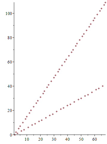
Proposition 4.
Let be the Wythoff swap sequence, and . Then for all
Proof.
Equation (4) and Equation (5) yield
Since by Equation (1), it follows from Equation (6) that
Since all will occur, this gives the first half of the proposition.
For the second half of the proposition we perform the following computation under the assumption that :
Now Equation (7) gives that . ∎
3 Generalizations
There is a lot of literature on generalizations of Hofstadter’s recursion . In most cases there is no simple description of the sequences that are generated by such recursions. An exception is the recursion analysed by Balamohan et al. [4]. The sequence with initial values 1,1,1,1 generated by this recursion is sequence A063882. Allouche and Shallit [2] prove that the ‘frequencies’ of this sequence can be generated by an automaton. See the recent paper [7] for more results on this type of Hofstadter’s recursions, known as Hofstadter Q-sequences. We consider the paper [6], that gives a direct generalization of Hofstadter’s G-sequence.
Theorem 6.
[Celaya and Ruskey] Let , and let .
Assume for , and for , let
Then for , .
As an example, we take the case . In that case , the small silver mean. The recursion for what we call the Hofstadter Pell sequence is
Here Theorem 6 gives that
This is sequence A097508 in OEIS.
Let and form the Beatty pair given by Theorem 1. Let and be the associated Beatty sequences. One has , and .
According to Theorem 2, with the slow Beatty sequence A049472 given by , the following holds for the Hofstadter Pell sequence :
The sequence with and swapped is
A109250 .
Apparently there is nothing comparable to the averaging phenomenon that occurred in the golden mean case.
4 Greediness
There is a more natural way to define the Wythoff swap sequence , which at first sight has nothing to do with Wythoff sequences.
Venkatachala in the paper [17] considers the following greedy algorithm:
, and for is the least natural number such that
Surprisingly, it follows from Venkatachala’s analysis that one has for all
The recent paper [3] studied a sequence defined by a similar greedy algorithm:
, and for is the least natural number such that
This entails that , defined by for , is a sequence of integers.
These sequences have been analysed by Shallit in the paper [12] using the computer software Walnut. Our Theorem 9 is an improvement of [12, Theorem 6]. In the proof of Theorem 9 we need the values of the Wythoff sequences at the Fibonacci numbers.
Lemma 8.
Let and be the Wythoff sequences. Then for all
| (8) | ||||
| (9) | ||||
| (10) | ||||
| (11) |
Proof.
These equations can be derived from [3][Lemma 2.D]. Another, easy, proof is based on recalling that gives the position of the in the infinite Fibonacci word generated by the morphism (see, e.g., [1, Corollary 9.1.6]). The infinite Fibonacci word is the limit of the words .
Let , , and denote the length, the number of 0’s and the number of 1’s of a word . Then it is easy to see that
| (12) |
for all , where is the iterate of . Since ends in for odd , Equation (12) with implies that Equation (8) holds. Similarly, since ends in for even , one obtains Equation (9). That Equation (10) is correct follows from Equation (12) with , since ends with for odd . Similarly, since ends with for odd , one obtains Equation (11) with . ∎
Theorem 9.
Let and be the Avdivpahic and Zejnulahi sequences. Let be the Wythoff swap sequence. Then for all
| In fact, | |||
| In fact, |
Proof.
Part (a). We use the formula for proved in the paper [3]:
So is the swapping of and for indices and . We first handle the case of the Fibonacci numbers with an odd index. Here we have to prove that
| (13) | ||||
| (14) |
We start with Equation (13). We have to show that there exists such that either the pair of equations , and , or the pair of equations , and holds. The first pair of these swapping equations, with the value , is equal to the equations (8), and (9), as we see from Lemma 8.
Next, we prove Equation (14). Here Lemma 8 gives that Equation (11) and Equation (10) solve the swapping equations.
We still have to handle the case with Fibonacci numbers with an even index. There we have to prove that
| (15) | ||||
| (16) |
We start with Equation (16). Here Lemma 8 gives that Equation(10) and Equation(11) solve the swapping equations.
Next, we prove Equation (15). Here Lemma 8 gives that Equation (8) and Equation(9) solve the swapping equations, both with shifted by 1.
Part (b). The case : for , and .
For we have
We see that for , and .
So also
Note furthermore that and
Since these two sums are equal, the difference of 1 created at is ‘repaired’ at . This proves the first part of Part b).
For the second part we have to see that , or equivalently (see the proof of the first part of Part (b)), that .
Let defined by the recurrences be the “married” functions of Hofstadter given in his book [10, p. 137]. Here is A005378 and is A005379.
Theorem 10.
[Stoll][16] Let and be the “married” sequences of Hofstadter. Let be the small golden mean. Then for all
5 Acknowledgment
I thank Jean-Paul Allouche for useful remarks. Thanks are also due to one referee for pointing out an important reference, and to a second referee for many remarks that have resulted in an improvement of the presentation.
References
- [1] J.-P. Allouche and J. Shallit, Automatic Sequences: Theory, Applications, Generalizations, Cambridge University Press, 2003.
- [2] J.-P. Allouche and J. Shallit, A variant of Hofstadter’s -sequence and finite automata, J. Aust. Math. Soc. 93 (2012), 1–8. doi:10.1017/S1446788713000074
- [3] M. Avdispahić and F. Zejnulahi, An integer sequence with a divisibility property, Fib. Quart. 8 (2020), 321–333.
- [4] B. Balamohan, A. Kuznetsov, and S. Tanny, On the behavior of a variant of Hofstadter’s Q-sequence, J. Integer Seq. 10 (2007), Article 07.7.1.
- [5] S. Beatty, Problem 3173, Amer. Math. Monthly 33 (1926), 159. Solutions, ibid., 34 (1927), 159.
- [6] M. Celaya and F. Ruskey, Morphic words and nested recurrence relations, arxiv preprint arXiv:1307.0153v1 [math.CO], 2013. Available at https://arxiv.org/abs/1307.0153.
- [7] N. Fox, Connecting slow solutions to nested recurrences with linear recurrent sequences, J. Difference Equ. Appl. 10 (2022), 1–34.
- [8] D. Gault and M. Clint, “Curiouser and curiouser” said Alice. Further reflections on an interesting recursive function, Internat. J. Computer Math. 26 (1988), 35–43.
- [9] V. Granville and J.-P. Rasson, A strange recursive relation, J. Number Theory 30 (1988), 238–241.
- [10] D. R. Hofstadter. Gödel, Escher, Bach: An Eternal Golden Braid. Basic Books, 1979.
- [11] C. Kimberling and K. B. Stolarsky, Slow Beatty sequences, devious convergence, and partitional divergence, Amer. Math. Monthly 123 (2016), 267–273.
- [12] J. Shallit, Proving properties of some greedily-defined integer recurrences via automata theory, arxiv preprint arXiv:2308.06544v1 [cs.DM], 2023. Available at https://arxiv.org/abs/2308.06544.
- [13] J. Shallit, Proof of Irvine’s Conjecture via Mechanized Guessing, arxiv preprint arXiv:2310.14252 [math.CO], 2023. Available at https://arxiv.org/abs/2310.14252.
- [14] N. J. A. Sloane et al., On-Line Encyclopedia of Integer Sequences, electronically available at https://oeis.org, 2023.
- [15] K. Stolarsky, Beatty sequences, continued fractions, and certain shift operators, Can. Math. Bull. 19 (1976), 473–482. doi:10.4153/CMB-1976-071-6.
- [16] T. Stoll. On Hofstadter’s married functions. Fib. Quart. 46/47 (2008/9), 62–67.
- [17] B. J. Venkatachala, A curious bijection on natural numbers, J. Integer Seq. 12 (2009), Article 09.8.1.
- [18] W. A. Wythoff, A modification of the game of Nim, Nieuw Arch. Wiskd. (2), 7 (1907), 199–202.
2020 Mathematics Subject Classification: Primary 05A17, Secondary 68R15
Keywords: Hofstadter’s G-sequence, slow Beatty sequence, Wythoff sequence.