Polyakov blocks for the 1D CFT mixed correlator bootstrapPreprint: APS/123-QED
Abstract
We introduce manifestly crossing-symmetric expansions for arbitrary systems of 1D CFT correlators. These expansions are given in terms of certain Polyakov blocks which we define and show how to compute efficiently. Equality of OPE and Polyakov block expansions leads to sets of sum rules that any mixed correlator system must satisfy. The sum rules are diagonalized by correlators in tensor product theories of generalized free fields. We show that it is possible to do a change of a basis that diagonalizes instead mixed correlator systems involving elementary and composite operators in a single field theory. As an application, we find the first non-trivial examples of optimal bounds, saturated by the mixed correlator system in the theory of a single generalized free field.
.0.1 Introduction and setup
Conformal theories in one dimension are interesting both in theory and in practice. On the one hand, they have a wide range of applications: from conformal defects to boundary conditions in 2d CFT, passing through 2d QFTs in AdS space and long range spin models, not to mention that in a sense, any CFT is a 1d CFT Billó et al. 2013; Gaiotto et al. 2014; Cuomo et al. 2022a; Cuomo et al. 2022b; Gimenez-Grau et al. 2022; Antunes et al. 2021; Paulos et al. 2017; Homrich et al. 2019; Knop and Mazac 2022; Córdova et al. 2022. On the other, being confined to a line and lacking spin, such theories have greatly simplified kinematics, while being far from elementary toy models, as there is no known non-trivial example which has been exactly solved. Thus these systems offer both a challenge as well as opportunity for significant progress in the conformal bootstrap program.
At its heart this program is about understanding how crossing equations constrain sets of CFT data, both analytically and numerically. As it turns out, working with such equations in their original formulation in position space is far from optimal for the purpose of deriving such constraints. Instead, work in recent years suggests one should apply a certain transform from position space onto an auxiliary functional space Mazac and Paulos 2019a; Mazac and Paulos 2019b. By construction, this mapping is done in such a way that crossing equations become translated into a completely equivalent set of sum rules which are now transparently solved by particular sparse sets of CFT data, something which is completely obscured in position space. Since all sets of CFT data, sparse or not, obey a measure of universality for large scaling dimensions Pappadopulo et al. 2012; Qiao and Rychkov 2017, these sum rules naturally give rise to a decoupling between low and high energy data, leading to rapidly convergent bounds and constraints Paulos and Zan 2020.
Up to now constructions of such functional spaces have been limited to systems of correlation functions of operators lying in the same symmetry multiplet Ghosh et al. 2021. This is a major restriction, as it is known that many CFTs of interest can only be effectively bootstrapped by considering systems of correlations functions involving distinct operator multiplets, the most famous example being the celebrated 3d Ising island El-Showk et al. 2012; El-Showk et al. 2014; Kos et al. 2014. In this paper we will resolve this shortcoming for 1d CFTs, by constructing new sets of sum rules valid for arbitrarily large systems of bootstrap equations. Our approach is to propose a generalization of the so-called Polyakov bootstrap to a multi-correlator setup Polyakov 1974; Gopakumar et al. 2017a; Mazac and Paulos 2019a; Mazac and Paulos 2019b; Gopakumar and Sinha 2018; Gopakumar et al. 2021; Ghosh et al. 2021. Contrary to previous work, this allows us to bypass the labourious construction of functional kernels which implement the above mentioned transform, obtaining instead the relevant sum rules directly. The price to pay is that one cannot rigorously prove that these sum rules are really equivalent to the constraints of crossing. In the present work we will settle for checking that our sum rules pass several highly non-trivial consistency checks, giving us enough confidence to begin using them for both analytic and numeric explorations. In both cases we show they significantly outperform traditional approaches, leading to new qualitative and quantitative insights into the structure of crossing equations and the systematics of bootstrapping 1d CFTs.
Setup — After these remarks, let us begin by recalling some basic facts and establishing notation. We are interested in 1d CFTs with primary operators labeled generically as . Conformal invariance dictates a correlation function can be expressed as a function of a single cross-ratio . Using the OPE (or simply ), we obtain an expansion for :
| (1) |
The sum runs over all primary operators labelled by their scaling dimension and spacetime parity . Here and is the 1d conformal block, see eq. (6) in supplementary materials 11 1 See supplementary materials (which includes ref. D’Hoker et al. 1999; Dolan and Osborn 2004; Zhou 2019; Gopakumar et al. 2017b; Mack; Mack 2009; Mazac 2017) for further details on Witten diagrams, bootstrapping the system of decoupled GFF scalars and the system, and numerical evidence of particle production..
For a system of mixed correlators we find it useful to introduce the “OPE orientation vector” , a new set of quantum numbers such that and , which describes how couples to different pairs of operators. We may then rewrite (1) as
| (2) |
with .
An important property of a four-point correlator is crossing symmetry. The OPE decomposition given by (2) is not manifestly crossing symmetric, as conformal blocks are associated to a particular OPE channel. To remedy this we introduce the Polyakov block expansion: Polyakov 1974; Gopakumar et al. 2017a; Mazac and Paulos 2019b
| (3) |
By construction, the Polyakov blocks are built to manifestly satisfy crossing. In particular, while in (2) the only operators which give a non-zero contribution are those in the -channel OPE , the Polyakov block sum receives contributions also from the OPE channels and . The price to pay for this representation is that term by term the OPE contains contributions from unphysical states which must decouple in the full sum. Concretely, the Polyakov bootstrap is the statement:
| (4) |
This should be thought of as a reformulation of the constraints of crossing symmetry, which has to be satisfied by any system of correlators in any CFT. We will shortly show how these bootstrap equations may be turned into a more useful discrete set of sum rules on the CFT data by using the OPE decomposition of the Polyakov blocks.
As functions, Polyakov blocks can be computed as sums of Witten diagrams. Starting off with the theory of decoupled free fields in AdS2, the associated boundary correlators correspond to those of the tensor product theory of generalized free fields (GFF) . Introduce now a new spin-0 bulk field with mass and dual operator of positive parity 22 2 Positive parity is reflected in the fact that . In AdS2 a negative parity operator on the boundary couples instead to a (massive) bulk spin-1 field, for which ., with couplings:
| (5) |
Then to leading order, the connected correlators in this theory are essentially proportional to the Polyakov block with the right quantum numbers, including the OPE orientation . We emphasize that this construction is simply a convenient recipe for computing the Polyakov blocks as functions: the constraints (4) are meant to hold for all CFTs and not just those arising from weakly coupled fields in AdS2.
.0.2 Sum rules
Since Polyakov blocks correspond to deformations of generalized free correlators, their OPE content consists of double trace operators, whose schematic form and scaling dimensions are given as:
| (6) | ||||||
At this point it is convenient to introduce some notational shorthand. We will denote a set of external fields by a letter (for External). We will also denote by (for Internal channel) a generic double trace operator appearing in the OPE channel . A given is always with respect to some particular . As an example, for we have
| (7) |
Similarly we denote and for the double traces and respectively. The negative parity channels are obtained from the above by swapping round and square brackets. We will also denote , and so on. Finally, we set
| (8) |
and similarly and .
After these notational preliminaries we are ready to discuss the OPE for Polyakov blocks Note1. As mentioned, they can be written as sums of Witten diagrams in AdS2, which include both exchanges and contact diagrams. Exchange diagrams have conformal block decompositions as follows Gopakumar and Sinha 2018; Penedones 2011:
| (9) |
where parity of the exchanged operator (even,odd) corresponds to the bulk spin respectively. The coefficients appearing above satisfy the orthogonality properties
| (10) |
As for contact diagrams, their block expansions take the form
| (11) |
The Polyakov blocks are then given as
| (12) |
We will fix the contribution of contact diagrams momentarily. Using the OPE and commuting sums, the Polyakov bootstrap equations become a set of conditons on OPE data which can be written as follows: Functional sum rules — For all there is a functional with the sum rule
| (13) |
The coefficients appearing in these sum rules are the functional actions. They satisfy a set of duality properties following the orthogonality relations (10). A slight issue arises when we have , for instance in a correlator . In that case some coefficients in the Witten exchange diagram OPE expansion are degenerate Note1, and we must make the replacements
| (14) |
and similarly for . The duality properties are then (writing , etc)
| (15) | |||||
The sum rules and duality relations have an implicit dependence on the contact diagrams as described below. Ignoring this part, there is one sum rule per label and per choice of .
Finally, let us discuss how to fix contact diagrams. Our guiding principle is that the sum rules should bootstrap solutions to crossing with the same UV, or Regge behaviour, as ordinary CFT correlators Mazac and Paulos 2019b; Ferrero et al. 2020. In AdS2 such solutions can be contact diagrams arising from relevant deformations in the bulk theory i.e. four-point interactions with at most two bulk derivatives. So for each choice of external states we include all such independent contact diagrams in the Polyakov block (12). We also require that we lose as many sum rules from (13) as there are contact diagrams. For example, for a certain choice of external states if there is only one independent contact diagram for all the possible permutations, then we would redefine
| (16) | ||||
where corresponds to some definite permutation of the indices in . The above eliminates the functional , as well as the corresponding duality relations. This procedure is such that by construction, contact diagrams are now manifest solutions to the sum rules. For notational clarity, below we will leave the subtraction procedure implicit.
.0.3 Basis change and optimal bounds
The , system — The duality relations (10) imply that the functional sum rules trivialize on a set of correlators of decoupled GFF scalars Note1. As a more interesting application, here we will examine how to bootstrap the system in a single GFF theory. In our language, this is the following system of unitary CFT correlators of fields and with dimensions :
| (17) |
with the GFF correlator (see (25) in Note1). There is a symmetry under which and are odd and even respectively. It is straightforward to expand the above in conformal blocks to extract the CFT data.
Let us discuss how the same data is reproduced using our sum rules. We include in all OPE channels all possible single and double trace operators consistent with the symmetry. To allow for possible degeneracies we introduce the notation . We then must impose the non-degeneracy conditions:
| (18) |
These tell us that there are unique operators with dimensions or respectively. Note that these conditions cannot be derived, but rather must be imposed as inputs which fix the solution to be bootstrapped (i.e. there are solutions to crossing where they are not true Note1). We can now determine all other OPE coefficients. In particular, the , sum rules determine the OPE coefficients , and respectively in terms of . Similarly, using the are also determined and come out zero as expected. At this point we use the nondegeneracy condition and now the remaining OPE data can be solved for using the and sum rules. Our results match those extracted from the correlators above, giving a non-trivial check of our sum rules.
Basis change — A dissatisfying feature of the last computation was that the basis of sum rules was not entirely diagonal with respect to the solution. Indeed the equations in channel involve an infinite number of variables, and have to be solved after the and channels . Here we will construct a new functional basis that does not suffer from this problem. Consider the functionals . We will construct modified versions, satisfying the following duality conditions:
| (19) | ||||||
Similar equations can be written for , by moving the Kronecker delta to the right column. These conditions are understood as follows. The first line are the original conditions satisfied by the functionals. Adding the second line implies that the new functionals now have (double) zeros acting on the operators — recall this means evaluating the functionals on the right dimensions and OPE orientation, and in this case we mean the operator for the system. Finally the last line guarantees that these vanishing conditions are still true under small deformations of the OPE orientation. Essentially the second and third lines ensure that the functional does not change sign in the neighbourhood of its zeros. While these two extra sets of conditions are not necessary for diagonalizing the bootstrap equations for the mixed GFF solution, they do allow to have diagonal equations even slightly away from this solution.
In practice the new duality conditions can be satisfied by setting:
| (20) |
and tuning coefficients appropriately. The same procedure can be applied to .
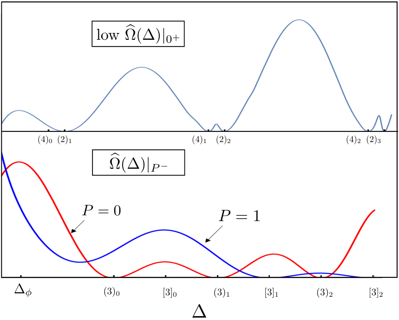
An optimal bound — We will now show that using a functional closely related to the above we can obtain an optimal bound satisfied by GFF. Let us consider the same setup as before, with operators labeled by their () and spacetime parity ( for even/odd) quantum numbers, e.g. etc. We set and with dimensions and charges as before. We assume that and are unique and also the leading non-identity operators, and fix the OPE data of the operator, (i.e. ) to the GFF values, which with the uniqueness assumption i.e. (18) also fixes . Our analytic bound is more simply stated for , which we do here, leaving further discussion to Note1. In this case our last assumption is that in the sector there should be no other operators below a gap no smaller than , apart from .
Under these assumptions, consider a operator denoted and of dimension . Then we claim there is an upper bound on which is saturated by the GFF solution. To prove this bound we first define . For any we can now “dress” this functional so that it is orthogonal to states in the 11 OPE. Specifically, we add to an infinite sum as in (20) and impose most of the duality conditions (19) except the one involving the state to obtain a new dressed functional . We find that for suitable choices of in some range is positive semidefinite for scaling dimensions consistent with the gap assumptions above, see figure 1. Thus it leads to a bound
| (21) |
To understand the equality, note that by construction annihilates every operator appearing in the GFF solution, except for and . This implies that for that solution the above inequality becomes an identity, i.e. the bound is saturated. To show this it is important to note that in the GFF solution there is no operator (it is , a descendant), otherwise would be sensitive to it.
To conclude, let us make a few comments on our assumptions. It may seem surprising that we need to impose a gap in the even sector even after completely fixing the data of . Indeed, a non-trivial but true fact is that fixing this data to its GFF values already implies that the entire 11 OPE must be that of a GFF Mazac and Paulos 2019b. It is easy to see that this means that the 1111 and 1122 four-point functions are automatically the same as the GFF ones, and that the double traces appear in the 22 OPE with their GFF OPE values. However, at this point the 22 OPE is still not fully constrained. Maximizing the OPE of the operator fixes it to become that of the GFF solution, but only under our gap assumption in the sector – OPE bounds generally require a minimal gap, otherwise the maximum is infinite.
.0.4 Numerical explorations: islands with GFF inhabitants and particle production
In this section we perform some preliminary numerical explorations using our setup 33 3 We used SDPBSimmons-Duffin 2015 software to solve the optimization problem involving mixed correlators., leaving more detailed computations for future work. In figure 2 we explore again the same mixed correlator system as before looking for the feasible region in the plane i.e. the OPE data of the operator 44 4 In Antunes et al. 2021 this was also explored using traditional bootstrap methods..
The island shown appears when we set gaps in the odd sectors. In particular in the figure we have set these to be in parity even (odd) channels respectively. When the gap is smaller, say in , we observe a region where the left direction of the plot is qualitatively similar, while on the right, it extends to a strip-like shape without any upper bound for , as found in Antunes et al. 2021. Conversely, larger gaps further shrink the allowed region.
The island displays two seemingly flat regions in the bottom and top, which are not numerical artifacts. In fact they are well described by single correlator bounds on . This suggests that the 11 OPE is unchanged along these boundaries. On the top, the bound is simply i.e. the GFF value. When we examine the spectrum of the extremal solution corresponding to the top right corner of the feasible region, we find a solution consistent with a non-interacting (GFF) 11 and 12 OPEs and an interacting 22, see figure 1 in the supplementary material. As explained there, this can be thought of as a consequence of the existence of a deformation in AdS2 which allows to deform the 22 OPE while holding the 11 fixed. While in this special case the 11 OPE remains free, the general result is that it should not only become interacting but also manifest “particle production”, i.e. couplings to the operators. An example is shown in Fig. 2 of the supplementary material.
Discussion and outlook
In this paper we have introduced a presumably complete reformulation of crossing symmetry constraints for an arbitrary set of 1d CFT correlators. Our sum rules are naturally adapted to study deformations of generalized free fields, allowing us to bridge the gap between analytic and numeric computations and promising to help us pinpoint desired theories to bootstrap. Our initial numerical explorations, which will be developed elsewhere, show not only greatly improved speed of convergence relative to traditional bootstrap methods, but much greater accuracy, allowing us to give precise spectra for interacting CFT solutions with features like “particle production” or lack thereof. Our methods thus promise to push the bootstrap into much larger sets of mixed correlators and probe the high energy asymptotics of CFT correlators. We will return to these questions in the very near future.
Acknowledgements.
We are grateful for discussions with Romain Usciati, Nat Levine, Antonio Antunes, Zechuan Zheng. A.K. is supported by DFG (EXC 2121: Quantum Universe, project 390833306). This work was co-funded by the European Union (ERC, FUNBOOTS, project number 101043588). Views and opinions expressed are however those of the author(s) only and do not necessarily reflect those of the European Union or the European Research Council. Neither the European Union nor the granting authority can be held responsible for them.References
- Billó et al. (2013) M. Billó, M. Caselle, D. Gaiotto, F. Gliozzi, M. Meineri, and R. Pellegrini, Line defects in the 3d Ising model, JHEP 07, 055, arXiv:1304.4110 [hep-th] .
- Gaiotto et al. (2014) D. Gaiotto, D. Mazac, and M. F. Paulos, Bootstrapping the 3d Ising twist defect, JHEP 03, 100, arXiv:1310.5078 [hep-th] .
- Cuomo et al. (2022a) G. Cuomo, Z. Komargodski, and M. Mezei, Localized magnetic field in the O(N) model, JHEP 02, 134, arXiv:2112.10634 [hep-th] .
- Cuomo et al. (2022b) G. Cuomo, Z. Komargodski, and A. Raviv-Moshe, Renormalization Group Flows on Line Defects, Phys. Rev. Lett. 128, 021603 (2022b), arXiv:2108.01117 [hep-th] .
- Gimenez-Grau et al. (2022) A. Gimenez-Grau, E. Lauria, P. Liendo, and P. van Vliet, Bootstrapping line defects with O(2) global symmetry, JHEP 11, 018, arXiv:2208.11715 [hep-th] .
- Antunes et al. (2021) A. Antunes, M. S. Costa, J. a. Penedones, A. Salgarkar, and B. C. van Rees, Towards bootstrapping RG flows: sine-Gordon in AdS, JHEP 12, 094, arXiv:2109.13261 [hep-th] .
- Paulos et al. (2017) M. F. Paulos, J. Penedones, J. Toledo, B. C. van Rees, and P. Vieira, The S-matrix bootstrap. Part I: QFT in AdS, JHEP 11, 133, arXiv:1607.06109 [hep-th] .
- Homrich et al. (2019) A. Homrich, J. a. Penedones, J. Toledo, B. C. van Rees, and P. Vieira, The S-matrix Bootstrap IV: Multiple Amplitudes, JHEP 11, 076, arXiv:1905.06905 [hep-th] .
- Knop and Mazac (2022) W. Knop and D. Mazac, Dispersive sum rules in AdS2, JHEP 10, 038, arXiv:2203.11170 [hep-th] .
- Córdova et al. (2022) L. Córdova, Y. He, and M. F. Paulos, From conformal correlators to analytic S-matrices: CFT1/QFT2, JHEP 08, 186, arXiv:2203.10840 [hep-th] .
- Mazac and Paulos (2019a) D. Mazac and M. F. Paulos, The analytic functional bootstrap. Part I: 1D CFTs and 2D S-matrices, JHEP 02, 162, arXiv:1803.10233 [hep-th] .
- Mazac and Paulos (2019b) D. Mazac and M. F. Paulos, The analytic functional bootstrap. Part II. Natural bases for the crossing equation, JHEP 02, 163, arXiv:1811.10646 [hep-th] .
- Pappadopulo et al. (2012) D. Pappadopulo, S. Rychkov, J. Espin, and R. Rattazzi, OPE Convergence in Conformal Field Theory, Phys. Rev. D 86, 105043 (2012), arXiv:1208.6449 [hep-th] .
- Qiao and Rychkov (2017) J. Qiao and S. Rychkov, A tauberian theorem for the conformal bootstrap, JHEP 12, 119, arXiv:1709.00008 [hep-th] .
- Paulos and Zan (2020) M. F. Paulos and B. Zan, A functional approach to the numerical conformal bootstrap, JHEP 09, 006, arXiv:1904.03193 [hep-th] .
- Ghosh et al. (2021) K. Ghosh, A. Kaviraj, and M. F. Paulos, Charging up the functional bootstrap, JHEP 10, 116, arXiv:2107.00041 [hep-th] .
- El-Showk et al. (2012) S. El-Showk, M. F. Paulos, D. Poland, S. Rychkov, D. Simmons-Duffin, and A. Vichi, Solving the 3D Ising Model with the Conformal Bootstrap, Phys. Rev. D 86, 025022 (2012), arXiv:1203.6064 [hep-th] .
- El-Showk et al. (2014) S. El-Showk, M. F. Paulos, D. Poland, S. Rychkov, D. Simmons-Duffin, and A. Vichi, Solving the 3d Ising Model with the Conformal Bootstrap II. c-Minimization and Precise Critical Exponents, J. Stat. Phys. 157, 869 (2014), arXiv:1403.4545 [hep-th] .
- Kos et al. (2014) F. Kos, D. Poland, and D. Simmons-Duffin, Bootstrapping Mixed Correlators in the 3D Ising Model, JHEP 11, 109, arXiv:1406.4858 [hep-th] .
- Polyakov (1974) A. M. Polyakov, Nonhamiltonian approach to conformal quantum field theory, Zh. Eksp. Teor. Fiz. 66, 23 (1974).
- Gopakumar et al. (2017a) R. Gopakumar, A. Kaviraj, K. Sen, and A. Sinha, Conformal Bootstrap in Mellin Space, Phys. Rev. Lett. 118, 081601 (2017a), arXiv:1609.00572 [hep-th] .
- Gopakumar and Sinha (2018) R. Gopakumar and A. Sinha, On the Polyakov-Mellin bootstrap, JHEP 12, 040, arXiv:1809.10975 [hep-th] .
- Gopakumar et al. (2021) R. Gopakumar, A. Sinha, and A. Zahed, Crossing Symmetric Dispersion Relations for Mellin Amplitudes, Phys. Rev. Lett. 126, 211602 (2021), arXiv:2101.09017 [hep-th] .
- (24) See supplementary materials (which includes ref. D’Hoker et al. 1999; Dolan and Osborn 2004; Zhou 2019; Gopakumar et al. 2017b; Mack; Mack 2009; Mazac 2017) for further details on Witten diagrams, bootstrapping the system of decoupled GFF scalars and the system, and numerical evidence of particle production.
- (25) Positive parity is reflected in the fact that . In AdS2 a negative parity operator on the boundary couples instead to a (massive) bulk spin-1 field, for which .
- Penedones (2011) J. Penedones, Writing CFT correlation functions as AdS scattering amplitudes, JHEP 03, 025, arXiv:1011.1485 [hep-th] .
- Ferrero et al. (2020) P. Ferrero, K. Ghosh, A. Sinha, and A. Zahed, Crossing symmetry, transcendentality and the Regge behaviour of 1d CFTs, JHEP 07, 170, arXiv:1911.12388 [hep-th] .
- (28) We used SDPBSimmons-Duffin 2015 software to solve the optimization problem involving mixed correlators.
- (29) In Antunes et al. 2021 this was also explored using traditional bootstrap methods.
- D’Hoker et al. (1999) E. D’Hoker, D. Z. Freedman, and L. Rastelli, AdS / CFT four point functions: How to succeed at z integrals without really trying, Nucl. Phys. B 562, 395 (1999), arXiv:hep-th/9905049 .
- Dolan and Osborn (2004) F. A. Dolan and H. Osborn, Conformal partial waves and the operator product expansion, Nucl. Phys. B 678, 491 (2004), arXiv:hep-th/0309180 .
- Zhou (2019) X. Zhou, Recursion Relations in Witten Diagrams and Conformal Partial Waves, JHEP 05, 006, arXiv:1812.01006 [hep-th] .
- Gopakumar et al. (2017b) R. Gopakumar, A. Kaviraj, K. Sen, and A. Sinha, A Mellin space approach to the conformal bootstrap, JHEP 05, 027, arXiv:1611.08407 [hep-th] .
- (34) G. Mack, D-independent representation of Conformal Field Theories in D dimensions via transformation to auxiliary Dual Resonance Models. Scalar amplitudes, arXiv:0907.2407 [hep-th] .
- Mack (2009) G. Mack, D-dimensional Conformal Field Theories with anomalous dimensions as Dual Resonance Models, Bulg. J. Phys. 36, 214 (2009), arXiv:0909.1024 [hep-th] .
- Mazac (2017) D. Mazac, Analytic bounds and emergence of AdS2 physics from the conformal bootstrap, JHEP 04, 146, arXiv:1611.10060 [hep-th] .
- Simmons-Duffin (2015) D. Simmons-Duffin, A Semidefinite Program Solver for the Conformal Bootstrap, JHEP 06, 174, arXiv:1502.02033 [hep-th] .
- (38) In general spacetime dimension these quantities depend on two cross ratios .
Appendix A Witten diagrams and functional actions
Here we will elaborate on the Witten diagrams in AdS2 and evaluating their conformal block expansions. In this work, we introduced two different kinds of Polyakov blocks corresponding to even or odd parity of the operator . They are given as sums of scalar or spin 1 exchange Witten diagrams respectively along with relevant Regge bounded contact diagrams. Below our strategy will be to compute these objects for general spacetime dimension and set at the end of the computation. Note that a general Witten diagram will depend on the spin of the exchange operator while in the dependence will be replaced with parity .
Expanding Witten diagrams in conformal blocks — For general spacetime dimension and scaling dimension and spin of an exchanged operator, -channel Witten diagrams are defined as D’Hoker et al. 1999,
| (22) |
where and are suitably normalized bulk to bulk and bulk to boundary propagators respectively. The corresponding crossed channel exchanged Witten diagram is obtained by swapping and the corresponding dimension of the external operator. So the -channel corresponds to the change of labels while the -channel corresponds to .
We want to compute conformal block decompositions of the 1d Witten diagrams. So we focus on only in the bulk which corresponds to respectively. They can be written in terms of a single cross-ratio 55 5 In general spacetime dimension these quantities depend on two cross ratios . as follows
| (23) |
Now this allows a conformal block decomposition that can be written as (denoting )
| (24) | ||||
| (25) | ||||
| (26) |
Here refers to the set of double trace operators . Also is the 1d conformal block given by
| (27) |
The coefficients can be obtained by using the Casimir operator to relate exchange Witten diagrams to contact diagrams as follows Zhou 2019; D’Hoker et al. 1999
| (28) |
Here is the conformal Casimir operator acting on and Dolan and Osborn 2004 and the corresponding eigenvalue for an operator with dimension and parity . In the righthand side is a combination of tree level contact diagrams which involve four scalar fields with a 4-point interaction vertex. Also is a normalization constant. Given that the maximum spin for the exchanged bulk operators is 1 for our case, the above relation leads to contact diagrams involving vertices with derivatives up to a maximum of second order. There are similar identities for any spin exchange Witten diagram in higher dimensions.
It is very easy to work out the block decomposition of any contact diagram from their simple form in Mellin space which we discuss below. Notice the Casimir operator acts on the -channel conformal block diagonally since blocks are eigenfunctions of Casimir. By applying the operator to the expression (24), we can extract the values of directly in terms of the conformal block decomposition of contact diagrams.
To obtain or i.e. the decomposition of the crossed channel exchange Witten diagram in the -channel conformal blocks, we employ a similar approach with the appropriate changes in the variables in (28). However, it is important to note that in the crossed channel, the action of the crossed channel Casimir on the direct channel conformal block is not diagonal. As a result, instead of obtaining a closed-form expression, we encounter a recursion relation for the coefficients of the decomposition Zhou 2019. This is very easy to implement numerically provided the seed block, i.e., the leading block decomposition coefficient or (for ). This we can obtain from the Mellin amplitude representation for the Witten diagrams Mack; Penedones 2011 which we describe below.
Witten diagrams in Mellin space — The Mellin amplitude of a general CFT correlation function can be defined by the inverse Mellin transform Gopakumar et al. 2017b:
| (29) |
where, , . Here are the conformal cross-ratios in general . The Mellin amplitude of -channel spin- exchange Witten diagram is given by
| (30) |
where the Mack polynomial is Mack; Mack 2009,
| (31) |
and
| (32) |
The -channel exchange Witten diagram is given by the following change of variables,
| (33) |
Similarly the -channel exchange Witten diagram is given by the following change of variables,
| (34) |
The Mellin ampllitude of the Regge-bounded contact diagrams is of the form ( are constants).
Let us now restrict to again. For this we will set in (29).
The seed conformal block that enters the recursion relation for crossed channel exchange Witten diagrams corresponds to the poles at or . The respective coefficient is obtained by computing the corresponding residue and then performing the integration. The result can be written in terms of a hypergeometric function Gopakumar and Sinha 2018.
Special case: integer differences in external dimensions — We end this appendix by commenting on the special case when differs from by an even integer. In this situation there is a pole in the conformal block decomposition coefficients . This comes from the factor like in the Mellin amplitude definition (29). Let us consider the following expansion explicitly
| (35) |
Here the ellipsis denotes other families of blocks appearing in the decomposition. When the expansion of the block decomposition coefficients near the pole looks like,
| (36) |
We will find that . This will give rise to derivative of blocks (denoting ) appearing in the expansion (35)
| (37) |
We also abuse the notation which now denotes the other piece . In other words, we get
| (38) | ||||
Appendix B Checks with analytical solutions
In section 2 of our main text we pointed out that the sum rules eq. (13) of main text trivialize on a set of correlators in a theory of decoupled GFF scalars. We also showed how the sum rules can bootstrap the system of and fields in GFF. In this appendix we will address the checks on both of these theories more elaborately and clarify the steps involved. For both these examples our general argument will be as follows: first we consider a set of mixed correlators that satisfy the crossing symmetry relation:
| (39) |
Then we will show how the sum rules solve the entire set of OPE data that is consistent with these correlators.
Tensor product theories — Our first test is that the sum rules correctly bootstrap correlators in a tensor product theory of several GFF operators. Thus we will set a fundamental generalized free field, and do not interact for . Let us explain how to bootstrap correlators in the tensor product theory of two bosonic fields of positive parity. They are given as
| (40) | ||||
Consider first the sum rules for . In this case the functional actions become
| (41) |
with and
| (42) |
The with are nothing but the functionals already introduced in Mazac 2017; Mazac and Paulos 2019a; Mazac and Paulos 2019b, so in this case our sum rules reproduce the ones derived there. More interestingly, consider the mixed correlators 12,12 and 11,22. The sum rules now are
| (43) |
with However, in this case there are two relevant contact diagrams possible, allowing us to make two subtractions. We choose them to eliminate the functionals and . With this caveat, let us check that the tensor product theory satisfies the sum rules. The operators appearing above are the identity, as well as double traces and . Furthermore each such operator always appears in a single OPE channel, which means the corresponding vector is essentially a Kronecker delta. We have then e.g.
| (44) |
Similarly we find . We have extensively checked that these results match those extracted from the actual CFT correlators. For we get
| (45) |
The righthand side is actually zero, yielding the expected result for in the tensor product theory. Finally, the sum rules are satisfied only if , which is indeed the case.
The system — The main application in section 2 of main text is to bootstrap a set of crossing symmetric CFT correlators built from the and GFF operators. This means we have two operators of dimension and whose correlators satisfy eq. (17) of the main text, which we repeat for convenience:
| (46) | ||||
There are two free parameters in these expressions, with different choices corresponding to different physical theories, so the sum rules will be unable to fix them. For instance we could set and in a theory of decoupled generalized free fields, and then . Setting corresponds to and become two decoupled GFF fields as in our previous example. Below we will focus on the case where and , with the exchanged field in the OPE identified with , and with . These correspond to imposing the two conditions:
| (47) |
To bootstrap these correlators we write down the most general OPE consistent with a symmetry and the double trace operator spectrum. Schematically:
| (48) | ||||
We begin by considering the mixed correlator constraints. The states in the 12 OPE are determined by:
| (49) |
and similarly for the parity odd ones. There are also equations. These turn out to be non-trivially satisfied thanks to the condition . Moving on, we also have equations:
| (50) |
and the righthand side is non-trivial. In particular one finds
| (51) |
consistently with the expected solution. For we get an equation analogous to (50), but now non-trivially the whole righthand side turns out to be zero, where again the condition is crucial. So we learn that as expected the states do not appear in the OPE. This means that the correlator contains only and is now easily bootstrapped as a fundamental GFF correlator:
| (52) |
Finally, this leaves us the equations for the correlator. These are
| (53) | |||
Imposing that the double trace spectrum contains non-degeneracies is the statement:
| (54) |
One can check that the equations are solved by this ansatz. In fact, turning the logic around, we should really think that they imply (54), so that these are not independent inputs. Finally the equations determine the coefficients .
Appendix C Further details on optimal and numerical bounds
In this appendix we will give further details on the analytic and numerical bounds discussed in the main text.
Optimal bound saturated by GFF —
Let us first discuss how the optimisation problem described in the main text must to be modified so as to be saturated by a GFF when . As mentioned there, our assumptions include the existence of an operator in the 11 OPE with the correct GFF OPE coefficient, and this in fact forces the entire 11 OPE to be that of a GFF. This, together with crossing for the 1122 correlator then implies that all operators also appear in the 22 OPE with their correct GFF coefficients. Thus at this point we can focus on understanding crossing for the 2222 correlator, keeping in mind the necessary presence of the identity and the tower of operators. The difficulty now is that from the point of view of crossing constraints for this correlator, on the one hand we know that we must demand a gap in the OPE of about otherwise there can be no upper bounds on any OPE coefficients; effectively this is because below this bound we can always add unitary solutions to crossing without identity to the correlator which can drive up OPE coefficients to arbitrarily large values. On the other, hand as increases, we know from our previous assumptions that there will definitely need to be some of the operators appearing below this gap. We must therefore allow at least those operators to appear, otherwise we would have inconsistent assumptions. To resolve this tension, the solution is to impose a general gap in the sector of about , but still allow a finite number of operators with dimension below it. Furthermore we must demand that any such operators are non-degenerate. In this way, only the operators which are forced by the 11 OPE constraints will appear and no others (which could appear just in the 22 OPE). In practice imposing these non-degeneracy conditions must be done by scanning in the OPE orientation space of these operators. The claim then is that our functional establishes that in this space there is a single feasible point precisely when these orientations match the ones of the GFF solution, and at that point there is a bound on given by the full GFF mixed correlator system.
Extremal spectra and particle production —
In the main text we showed an island in the space of OPE coefficients for the operator in a mixed correlator system. The top right corner of the island corresponds to setting the OPE data to match that of GFF. As discussed above we expect that in this case the and correlators to match the GFF result, but not necessarily that of . In figure 3 we examine the extremal spectrum corresponding to that corner, as obtained by looking for an upper bound on given . This spectrum is in perfect agreement with our expectations: the 11 OPE is indeed the GFF one, but we see that the 22 OPE is not. To see this had to be the case, simply note that if it the 22 OPE contained the GFF operators then the resulting extremal functional would need to have double zeros on all operators. But such a functional would rule out the existence of the bulk term, which can perturbatively modify the operators while keeping the unchanged.
Let us end this appendix with a small discussion on particle production. By particle production we mean interacting solutions where an OPE channel, say 11, starts seeing new families of operators, e.g. both and . We show such a solution in Fig. 4. It follows from an optimization problem (for ) to maximize the OPE coefficient of an operator with dimension in the presence of another operator in the OPE, with dimension and OPE coefficient .
This example demonstrates what is our general expectation, namely that a generic extremal solution to the mixed correlator bootstrap will necessarily have “particle production”. This just means that generically any operator that can appear in an OPE will do so. In particular, operators appearing in the 22 OPE must also appear in the 11 OPE and vice-versa. Intuitively this must be the case as to solve all the functional sum rules, in particular the mixed ones , we necessarily need to turn on all possible OPE coefficients. There are in fact special corners in the space of solutions exist where this doesn’t happen, GFF and minimal model correlators being prominent examples. It would be extremely interesting to find other ones.