The weak noise theory of the O’Connell-Yor polymer as an integrable discretisation of the nonlinear Schrodinger equation
Alexandre Krajenbrink
Email: alexandre.krajenbrink@quantinuum.comAffiliation: Quantinuum, Terrington House, 13–15 Hills Road, Cambridge CB2 1NL, United Kingdom
Affiliation: Le Lab Quantique, 58 rue d’Hauteville, 75010, Paris, France
Pierre Le Doussal
Email: ledou@lpt.ens.frAffiliation: Laboratoire de Physique de l’École Normale Supérieure, CNRS, ENS PSL University, Sorbonne Université, Université de Paris, 75005 Paris, France
August 11, 2026
Abstract
We investigate and solve the weak noise theory for the semi-discrete O’Connell-Yor directed polymer. In the large deviation regime, the most probable evolution of the partition function obeys a classical non-linear system which is a non-standard discretisation of the nonlinear Schrodinger equation with mixed initial-final conditions. We show that this system is integrable and find its general solution through an inverse scattering method and a novel Fredholm determinant framework that we develop. This allows to obtain the large deviation rate function of the free energy of the
polymer model from its conserved quantities and to study its convergence to the large deviations of the Kardar-Parisi-Zhang equation. Our model also degenerates to the classical Toda chain, which further substantiates the applicability of our Fredholm framework.
There has been much recent progress in obtaining exact solutions for the weak noise theory (WNT) of stochastic continuous systems in 1+1 dimensions.
This was achieved in the context of the Kardar-Parisi-Zhang (KPZ) equation
UsWNT2021; UsWNTFlat2021; TsaiIntegrability, introduced to describes interface growth KPZ,
and of the macroscopic fluctuation theory (MFT)
NaftaliDNLS; krajenbrink2023crossover; grabsch2021closing; mallick2022exact; NaftaliDNLS2; GrabschBenichou2023Review,
which describes diffusive particle systems BertiniPRL2005; DerridaGershenfeld; DerridaMFTReview2007; BertiniMFT2015.
The WNT describes the optimal configuration of height or density fields which realizes atypically large fluctuations in the presence of a weak noise
Korshunov; Baruch; lin2020short: this is an example of a large deviation problem TouchetteReview2018.
The progress was achieved by noticing that the nonlinear systems of equations which arise in WNT are integrable.
For the KPZ equation, where the WNT describes the short time regime, these equations are a close cousin of the nonlinear Schrodinger equation (NLS),
while for the MFT the connection is to the derivative nonlinear Schrodinger equation.
Both equations are integrable using the inverse scattering method
based on the existence of a Lax pair ZS; AblowitzKaup1974; kaup1978exact,
but solving the WNT requires handling mixed initial-final time conditions.
These connections to stochastic problems have renewed the interest in these classical integrable systems
due to the new challenge of non-standard mixed boundary conditions,
together with the possibility to solve exactly the equations using Fredholm determinants.
In fact, some of the large deviation rate functions obtained by these classical integrability methods
have also been derived le2016exact; krajenbrink2017exact; Meerson_flatST; krajenbrink2023crossover
from Fredholm determinant formula stemming from quantum integrability.
While complementary, the two approaches are quite distinct, and the connections between them
are not elucidated.
Figure 1: Example of a configuration of the O’Connell-Yor polymer, here for , where independent Brownian live on each horizontal line.
These studies have so far remained in the scope of continuous systems and the question whether this can be extended to discrete systems is still open. In this Letter, we provide a positive answer to this question in the context of the semi-discrete O’Connell-Yor (OY) polymer
o2001brownian; O_Connell_2002; O_Connell_2012, a discretization of the KPZ equation BorodinMacdo.
In its point-to-point version, it is defined by the partition sum defined as
(1)
The directed polymer path lives on the horizontal lines and jump upward from line to at
time , see Fig. 1. The are independent standard Brownian motions and represent the noise. The endpoints are fixed at and .
For this is just the geometric Brownian motion
much studied in the Black-Scholes model in finance bouchaud2003theory.
The weak noise limit amounts to take the (inverse temperature) parameter . Consider
first the simplest case of the geometric Brownian motion in the weak noise, i.e. small volatility, limit.
Although its typical fluctuations are simple
(they are Brownian by expanding the exponential), the large deviations are more interesting. Indeed
consider the observable
(2)
where overbar denotes expectation values with respect to the noise, and the
the rate function is
(3)
where is the Lambert function SM; corless1996lambertw.
Hence it is already non-trivial for and describes how the rare large
fluctuations affect the geometric
Brownian motion.
In this Letter, we consider such large deviation
observables for the full OY problem defined in Eq. (1) with arbitrary number of lines .
This now involves a non-trivial path-dependent optimization.
We show that these large deviations are controlled by a system of deterministic nonlinear equations with mixed initial-final boundary conditions which arise from the saddle point of the dynamical action associated to the stochastic evolution of . These equations are a discretization of the system studied by us using inverse scattering in the context of the KPZ equation in Refs. krajenbrink2021inverse; krajenbrink2022inverse; krajenbrink2023crossover - a close cousin of the NLS equation ZS, and a member of the
AKNS hierarchy AblowitzKaup1974. Interestingly it is a nonstandard discretisation, whose nonlinearity is local on the lattice, and which is closely related to other physical models such as the discrete self-trapping dimer model kuznetsov2000quantum; enol1991alternate, the Toda lattice
christiansen1993integrable,
and the periodic TASEP at large time SilvaPrivate. These equations are integrable in the sense of the existence of a Lax pair. Our contribution is the derivation of an inverse scattering theory adapted to boundary conditions which are non-local in time, together with the explicit solution of these equations in terms of direct and inverse scattering. This allows us to obtain the analytical expression of the large deviation rate function for the OY model for arbitrary as well as the optimal history of the partition function conditioned on the large deviations. We complement our study
by performing an asymptotic analysis of a determinantal formula obtained for the OY model BorodinMacdo; imamura2016determinantal, which
agrees with our results. We also show in detail how, in the limit of
large , these equations and their solutions recover the previous results for the Weak Noise Theory/short-time limit of the KPZ equation krajenbrink2021inverse.
As an amusing byproduct, we obtain a new contour integral representation of the Lambert function.
We start by recalling the coupled stochastic equations which are obeyed by the set of all the partition functions . It reads
(4)
in Ito discretization, where the are independent white noises,
and where
with the convention . Here
we are interested in the large deviation form of the cumulant generating function (CGF)
(5)
One of our aim is to compute the rate function explicitly for any . From it one
can extract the large deviation form of the PDF of of
(6)
through Legendre inversion of the saddle point
(7)
The calculation of the CGF is done using the path-integral representation
(8)
in terms of the dynamical action
(9)
where the source field is here , see SM.
In the limit we evaluate the r.h.s of (8) using
a saddle point method which leads to the following nonlinear differential equations
(10)
To study the point-to-point polymer one must impose the following initial and final conditions
(11)
Note that one also has for all , and for all . Also, for these boundary conditions, we expect the symmetry to hold.
Here is the lattice index and is the spectral parameter and is a 2-component vector. One can check that the original system (10) is recovered from the compatibility equation .
The general strategy that we use is to first solve the direct scattering problem
(12). In a second stage we give the general solution of the
inverse scattering problem and reconstruct the field
solution of the system (10). We first describe mathematically the general method to solve
the system (10),
before applying it to the specific boundary conditions (11) of interest for the polymer problem.
To this aim, let us denote with and two independent solutions of the linear Lax pair problem. Assuming that the fields vanish as ,
which is the case for the boundary conditions (11),
we can choose the solutions to behave asymptotically as and at . At , each solution should be a particular linear combination of these elementary solutions.
This allows to define the scattering amplitudes as
(14)
Inserting Eqs. (14) in the Lax equation with for yields the time-dependence of the scattering amplitudes , , and . Note that the representation of the Lax matrices (13)
chosen here is particularly convenient as and . As a consequence, the
Wronskian of is constant in space and time SM. This allows to
the obtain the following normalisation relation of the scattering amplitudes footnote-ablowitz-ladik
. We expect to be analytic inside a contour enclosing the origin which we choose as a
circle of radius , i.e. for , and
and to be analytic outside, i.e. for .
Although we will use that circle notation for simplicity, it is understood below in this work
that for (a large positive value defined later)
the circle must actually be deformed into an ellipse SM.
From the knowledge of the scattering amplitudes, it is possible to reconstruct explicitly the field using a novel
Fredholm operator formula that we now present. We first define the Fourier transforms of the ratio of scattering amplitudes called reflection coefficients as
(15)
(16)
where the contour integrals are taken over the -circle.
We then define two (space-time dependent) Hankel operators and with the following kernels
(17)
where the indices are positive . The product of two such operators is defined as
(18)
and we define the vector with component so that for any operator . Then the general solution of Eq. (10) reads
(19)
The additive structure present in Eq. (17) arises from the integrability of the problem and is akin to the structure for the continuous space problem krajenbrink2020painleve; krajenbrink2021inverse; bothner2022riemann. An analogous formula also exists for , see SM. Note that this formula (19) can be easily evaluated numerically using a discretized version of the Bornemann algorithm krajenbrink2021inverse.
Quite remarkably for the
boundary conditions of interest here (11), the calculation of the scattering amplitudes can be performed explicitly. Indeed, by solving
the spatial Lax equation and at and , see SM, one obtains
(20)
The normalisation relation then implies that
(21)
To obtain the expression of , , we solve Eq. (21) as a scalar Riemann-Hilbert (RH) problem.
There are two families, or branches, of solutions of Eq. (21) which are relevant for our large deviation
problem, i.e. needed to invert (7) to obtain .
Main branch, no solitons. The first family of solution does not involve solitons and determines the main branch of
. It assumes that has no zero for
and that has no zero for .
Solving the RH problem Eq. (21), see SM, one obtains
(22)
with
(23)
where is a closed contour around the origin which must avoid the branch cuts of the logarithm.
For most values of interest, , can be chosen as the circle .
The threshold is defined in SM, it grows very fast with (with ) and
plays little role below, so we stick to the circle notation. From the knowledge of the scattering amplitudes, one additionally obtains the values
taken by the conserved quantities of the problem, for details see SM. This is achieved by Laurent or Taylor expanding
the scattering amplitudes as
(24)
In particular, expanding equivalently
Eq. (23), we have that the value taken by the -th conserved quantity is
(25)
Since the first conserved quantity is related to the fields as
and is by definition time independent, it can be evaluated at where one has
(26)
thanks to the boundary conditions (11). From the derivative of (7) w.r.t. one sees that
. Hence the large deviation rate function is determined by the
first conserved quantity and one obtains
(27)
Note that for , Eq. (27) provides a novel integral representation of the Lambert function as from Eq. (3). A direct integration of (27) finally yields
(28)
where refers to the dilogarithm footnotecontour which domain of definition restricts the validity of this formula for
(29)
It allows to reconstruct the rate function with
in the range
(30)
and one obtains the parametric representation
(31)
for as .
This range contains which gives the typical value
,
as well as the second cumulant of the partition sum
, and of its logarithm
(32)
Second branch, with solitons. The second family of solution involves solitons, and allows to
obtain the rate function for the range ,
i.e. . To see how it arises consider the right hand side of Eq. (21). One can
check that for it has four zeroes
on the real axis with
(33)
and and . Here
and are the two main branches of the Lambert function corless1996lambertw.
The existence of these zeroes allows for a modified solution to the RH problem
(21), where has two zeroes inside the
-circle, , and two zeroes outside, . The solution then reads
(34)
with
(35)
where is given by the same formula as in (23).
By either Taylor or Laurent expanding the new solitonic contribution in (35), one also obtains an additional (solitonic) contribution to the values of the conserved quantities. In particular one
obtains which leads to the
following correction SM
(36)
It can be explicitly integrated over and we obtain the second branch
of the rate function with
(37)
where the solitonic contribution is
(38)
This second branch allows to reconstruct for ,
using the same parametric representation (31) where
now one replaces everywhere .
As increases from to , the values
of increase from to . The two branches
of are shown in Fig 2 where one sees that the branches merge smoothly.
Figure 2: Derivative of the rate function, . The main branch is in blue and the
second (solitonic) branch is in orange. The ordinate is also equal to hence one can
read off the relation between and (which is not one-to-one).
As we have obtained our solution for general , it is natural to study the limit when the polymer sees a large number of lines, i.e. . It is known that in the large limit the OY polymer point-to-point partition sum converges, under the proper rescaling, to the solution of the stochastic
heat equation, i.e. to the exponential of the KPZ height, for the so-called droplet initial conditions BorodinMacdo.
Here we can check that Eq. (5)
converges
to the corresponding equality for the KPZ equation at short time,
which was obtained in le2016exact; krajenbrink2021inverse.
To this aim we first define the
rescaled variables
(39)
where is the time in the KPZ equation. We then expand the formula (28)
for at large around the point on the contour,
by setting which yields for large
(40)
where
(41)
is the rate function for the KPZ equation with droplet initial data. Equation (40) shows
the convergence of the r.h.s of (5) and the convergence
of the l.h.s of (5) is obtained using
Ref. (BorodinMacdo, Section 5.4.1), which allows to
identify at large
(42)
where is the properly shifted KPZ height field,
denoted in krajenbrink2021inverse. To control the convergence of the solitonic branch, we expand the Lambert functions around
in (38) and obtain SM
(43)
This shows the convergence to the corresponding solitonic branch of the KPZ equation,
obtained in krajenbrink2021inverse (see also TsaiIntegrability). For completeness, we have also derived the above results for
from an asymptotic analysis of a determinantal representation formula for
BorodinMacdo; imamura2016determinantal using a first cumulant approximation,
see details in SM.
The OY polymer is also related to the
quantum Toda lattice O_Connell_2012. Here we
show that its weak noise theory (10) converges to
the classical Toda lattice toda1967vibration in the small time limit. Indeed, using the Cole-Hopf parameterization
, ,
and taking we find
the Toda dynamics in scaled time SM
(44)
Hence our results on the scattering theory and on the Fredholm determinants apply,
extending known solutions for solitons bauhardt1987fredholm. Finally, there seems to exist a connexion between the weak noise theory of the OY polymer and an integrable spin chain which we discuss in SM.
In conclusion we have shown that the weak noise theory of the
OY polymer is integrable for any , obtained its general solution
in terms of Fredholm determinants, and computed large deviation rate functions
from conserved quantities. The system (10)
provides a discretization of the NLS equation with local nonlinearity
and converges at large to the weak noise of the KPZ equation.
A distinct limit is the classical Toda chain, which is related to the QR decompositions in linear algebra symes1982qr; deift1983ordinary,
hence the extension to our system may
provide applications to linear algebra algorithms.
Finally, this work opens the path for a general study of weak noise limit in stochastic integrable systems and their connection to classical integrability. Since semi-discrete integrable systems have found renewed interest given their connexions to random matrix theory grava2023discrete; mazzuca2023equilibrium; spohn2020generalized; spohn2021hydrodynamic; spohn2022hydrodynamic, the model studied in this work will find additional applications. A potential outcome of this general study might lead to a broader classification of stochastic integrable models.
Acknowledgements.
Acknowledgments.
AK thanks Guilherme L. F. Silva for discussions on the existence of the Lax pair for the equations (10). We thank Alexei Borodin for interesting discussions and collaborations on
closely related topics. We acknowledge support
from MIT-France MISTI Global Seed Funds project “Exact Solutions in Field Theories via Integrable Probability”
and the MIT math department for hospitality. PLD acknowledges support from the ANR grant ANR-17-CE30-0027-01 RaMaTraF.
References
(1) A. Krajenbrink and P. Le Doussal.
Inverse scattering of the Zakharov-Shabat system solves the weak
noise theory of the Kardar-Parisi-Zhang equation.
Phys. Rev. Lett., 127 (6):064101, (2021).
(2) A. Krajenbrink and P. L. Doussal.
Inverse scattering solution of the weak noise theory of the
Kardar-Parisi-Zhang equation with flat and Brownian initial conditions.Physical Review E, 105(5):054142, (2022).
arXiv:2107.13497, (2021).
(4) M. Kardar, G. Parisi and Y-C. Zhang,
Dynamic Scaling of Growing Interfaces,
Phys. Rev. Lett. 56, 889, (1986).
(5) Bettelheim, Eldad, Naftali R. Smith, and Baruch Meerson.
Inverse Scattering Method Solves the Problem of Full Statistics of Nonstationary Heat Transfer in the Kipnis-Marchioro-Presutti Model.Phys. Rev. Lett. 128, 130602, (2021).
(6) A. Krajenbrink and P. Le Doussal.
Crossover from the macroscopic fluctuation theory to the
Kardar-Parisi-Zhang equation controls the large deviations beyond Einstein’s
diffusion.Physical Review E, 107(1):014137, (2023).
See also arXiv:2204.04720.
(7) A. Grabsch, A. Poncet, P. Rizkallah, P. Illien, and O. Bénichou.
Closing and solving the hierarchy for large deviations and spatial
correlations in single-file diffusion.
arXiv:2110.09269, (2021).
(8) K. Mallick, H. Moriya, and T. Sasamoto.
Exact solution of the macroscopic fluctuation theory for the
symmetric exclusion process.Phys. Rev. Lett. 129, 040601, (2022).
(9) E. Bettelheim, N. R. Smith, B. Meerson,
Full Statistics of Nonstationary Heat Transfer in the Kipnis-Marchioro-Presutti Model,
J. Stat. Mech. 093103, (2022).
(10) A. Grabsch, P. Rizkallah, A. Poncet, P. Illien, and O. Bénichou.
Exact spatial correlations in single-file diffusion.Physical Review E, 107(4):044131, 2023.
(11) L. Bertini, A. De Sole, D. Gabrielli, G. Jona-Lasinio, and
C. Landim,
Current Fluctuations in Stochastic Lattice GasesPhys. Rev. Lett. 94, 030601 (2005).
(12) B. Derrida and A. Gerschenfeld,
Current Fluctuations in One Dimensional Diffusive Systems with a Step Initial Density ProfileJ. Stat. Phys. 137, 978 (2009).
(14) L. Bertini, A. De Sole, D. Gabrielli, G. Jona-Lasinio and C. Landim,
Macroscopic fluctuation theory.
Reviews of Modern Physics, 87(2):593, (2015).
(15) I. V. Kolokolov, S. E. Korshunov,
Explicit solution of the optimal fluctuation problem for an elastic string in random potential.
Phys. Rev. E 80, 031107, (2009);
Universal and non-universal tails of distribution functions in the directed polymer and KPZ problems.
Phys. Rev. B 78, 024206, (2008);
Optimal fluctuation approach to a directed polymer in a random medium.
Phys. Rev. B 75, 140201, (2007).
(16) B. Meerson, E. Katzav, A. Vilenkin,
Large Deviations of Surface Height in the Kardar-Parisi-Zhang Equation,
Physical Review Letters 116, 070601, (2016).
(19) Shabat, A., and V. Zakharov.
Exact theory of two-dimensional self-focusing and one-dimensional self-modulation of waves in nonlinear media.
Soviet physics JETP 34.1 (1972).
(20) Ablowitz, M. J., Kaup, D. J., Newell, A. C., and Segur, H.
The inverse scattering transform-Fourier analysis for nonlinear problems.
Studies in Applied Mathematics, 53(4), 249-315, (1974).
(22) P. Le Doussal, S. N. Majumdar, A. Rosso, G. Schehr,
Exact short-time height distribution in 1D KPZ equation and edge fermions at high temperature,
Phys. Rev. Lett. 117, 070403, (2016).
(23) A. Krajenbrink, P. Le Doussal,
Exact short-time height distribution in the one-dimensional
Kardar-Parisi-Zhang equation with Brownian initial condition,
Phys. Rev. E 96, 020102, (2017).
(24) N. R. Smith and B. Meerson,
Exact short-time height distribution for the flat Kardar-Parisi-Zhang interface ,
Phys. Rev. E 97, 052110, (2018).
(29) J.-P. Bouchaud and M. Potters.
Theory of financial risk and derivative pricing: from
statistical physics to risk management.
Cambridge university press, (2003).
(32) A. Krajenbrink and P. Le Doussal.
Inverse scattering of the Zakharov-Shabat system solves the weak
noise theory of the Kardar-Parisi-Zhang equation.
Phys. Rev. Lett., 127 (6):064101, (2021).
(33) A. Krajenbrink and P. L. Doussal.
Inverse scattering solution of the weak noise theory of the
Kardar-Parisi-Zhang equation with flat and Brownian initial conditions.Phys. Rev. E 105, 054142, (2021).
(35) V. Enol’skii, M. Salerno, N. Kostov, and A. Scott.
Alternate quantizations of the discrete self-trapping dimer.Physica Scripta, 43(3):229, (1991).
(42) Note that this contrasts with the normalisation relation for the scattering amplitudes of the Ablowitz-Ladik which have an explicit dependence on the potentials , see SM. The Ablowitz-Ladik model is another semi-discrete integrable model related to the NLS equation. ablowitz2004discrete.
(51) G. Mazzuca, T. Grava, T. Kriecherbauer, K. T. McLaughlin, C. B. Mendl, and
H. Spohn.
Equilibrium spacetime correlations of the Toda lattice on the
hydrodynamic scale.arXiv:2301.02431, (2023).
(55) M. J. Ablowitz, B. Prinari, and A. D. Trubatch.
Discrete and continuous nonlinear Schrödinger systems,
volume 302.
Cambridge University Press, (2004).
(56) H. Spohn.
Hydrodynamic scales of integrable many-particle systems.
arXiv:2301.08504, 2023.
(60) V. E. Zakharov and L. A. Takhtadzhyan.
Equivalence of the nonlinear Schrödinger equation and the
equation of a Heisenberg ferromagnet.
Theoretical and Mathematical Physics, 38(1):17–23, (1979).
(61) Y. Angelopoulos, R. Killip, and M. Visan.
Invariant measures for integrable spin chains and integrable discrete NLS.arXiv:1807.08801, (2018).
(62) A. Krajenbrink, P. Le Doussal, Simple derivation of the large deviation tail for the 1D KPZ equation,
J. Stat. Mech. 063210, (2018).
(63) A. Krajenbrink, P. Le Doussal, S. Prolhac,
Systematic time expansion for the Kardar-Parisi-Zhang equation, linear statistics of the GUE at the edge and trapped fermions.
Nuclear Physics B, 936 239–305, (2018).
(64) Alexandre Krajenbrink.
Beyond the typical fluctuations: a journey to the large
deviations in the Kardar-Parisi-Zhang growth model.
PhD thesis, PSL Research University, 2019.
Supplementary Material for
The weak noise theory of the O’Connell-Yor polymer as an integrable discretisation of the nonlinear Schrodinger equation
We give the principal details of the calculations described in the main text of the Letter as well as additional information about the results.
Note that in the main text we use the notation for the OY partition sums (i.e. a random variable)
and for the solution of the weak noise saddle-point equations. Here we will simplify
notations and use the same letter for both, and the context will make it clear which is which.
I Model and observable
In this Supp. Mat. we will consider a slight generalization of the partition sums (1) defined in the text, which
corresponds to adding drifts to the Brownian weights . One thus defines for the partition function
(S45)
It is convenient to define , so that the first two terms read explicitly
(S46)
Using the rules of Ito calculus it is easy to see that these partition sums satisfy the following coupled stochastic equations
in Ito discretization for
(S47)
where the are standard independent
white noises, i.e. with correlators . One uses the
convention and the initial condition is .
The observable of interest is the partition function at one point and its probability distribution function
. It is useful to also introduce its logarithm and its PDF .
These PDF’s exhibit, in the weak noise limit the following large deviation
principle
(S48)
To compute these rate functions, which differ only by a change of variable,
we will first compute the following generating function of the cumulants of
(S49)
and the rate function . The two rate functions are related by the Legendre transform
(S50)
II Dynamical field theory and saddle point equations
We now use the standard path integral representation using source fields
(S51)
(S52)
where (and similarly for and ) is the
path integral measure, in terms of the dynamical action (time dependence is implicit)
(S53)
The source-less action reads
(S54)
where we have integrated over the noises . We have introduced the response field
to enforce the equations of motion. To obtain the observable in (S49) we
need to choose the source field .
In the limit the path integral (S52) is dominated by the saddle point of the action . The saddle point
equations take the form of the following system of equations
(S55)
We have added for convenience the parameter for the non-linearity, but for the application here one must set .
Note that a priori the above saddle point equations hold for . However, for technical reasons
it is useful to extend the system (S55) for all , which
we do from now on. We then consider the following initial and final conditions
(S56)
where imposing the last condition is equivalent to omitting the source term
in the equation of motion for . Note that one also has for all , and for all .
In practice we also take except if . Finally the response field vanishes for for all .
It is useful to note the following exact symmetry of the solution of the system (S55)
with the boundary conditions (S56).
If then
(S57)
We will obtain below the solution of this system of equations for any . Once this is done one can
insert the solution into the dynamical action to obtain its value at the saddle point. Hence one has
(S58)
Hence the PDF
of is given by the optimal action , which using
the saddle point equations simplifies into (for )
(S59)
evaluated using the solution of (S55) with , this determines . In practice however we will obtain as a function of
by solving (S55). From the Legendre
relation obtained by taking a derivative of (S50) w.r.t. ,
this will allow to determine . The last step will be to
obtain by an inverse Legendre transform.
We note that the evolution equations (S55) differ in part by the minus sign in front of the time derivative. This reflects that the evolution of can be seen as forward in time and the evolution of as backwards in time so that the whole problems is closer to a shooting problem rather than a dynamical problem.
III Two simple cases
III.1
Let us consider the system (S55) in the simple case
with the boundary conditions (S56). In this case the two equations decouple and
are simply linear. In the absence of drifts the solution is readily obtained as
(S60)
Figure S3: Solution of the problem without interaction, , as given in Eq. (S60).
In the presence of drifts it is easier to solve these equations using a Fourier representation
which will be useful in the following. Let us write
(S61)
where is a circle around in the complex plane. Inserting into
(S62)
for , it gives
(S63)
For we can solve directly
(S64)
Hence one has
(S65)
and the contour must include . Then we obtain for
(S66)
which gives for any (using that for )
(S67)
which automatically vanishes for . The contour must contain all the . Similarly one
has and one
obtains
(S68)
If we set all one can check that one recovers (S60).
III.2
For there are several ways to obtain the large deviation rate functions.
First method. For the system (S55) involves only the variables and
and becomes
(S69)
with and . The quantity is obviously conserved
so that where is a constant independent of time. Thus the system becomes
(S70)
and we find that and . The constant is thus determined by
(S71)
where is the Lambert function, such that . From the optimal action (S59) we obtain,
parametrically
(S72)
which leads to
(S73)
Second method.
Alternatively going back to the original stochastic model, where the partition sum for is simply
(here beware is not the solution of the SP equation)
one can compute directly its cumulant generating function, as sketched in the text. Indeed, denoting one has for small ,
(S74)
arising from events where the Brownian is anomalously large, i.e. .
Here we have, for
(S75)
There is a single minimum which is reached at
(S76)
which is seen to equal the constant of the first method. This gives
(S77)
as given in the text for . This gives also
.
Note that in agreement with the general
formula for conserved quantities (see Section VIII).
Although the function was defined and computed for the formula
(S77) can be continued to negative , on the principal branche , down to . This
is in agreement with the general formula for arbitrary obtained below which
states that
(S78)
Let us now discuss the Legendre transform which relates and .
One has
(S79)
leading to
(S80)
The typical value of is given by using that .
Using that we see that the domain corresponds to .
This is the principal branch with .
To obtain the values of one needs to consider a second branch.
This is achieved using the second real branch of the Lambert function, .
Then one has
(S81)
where increases again from back to , see
Appendix XI.3.
One obtains overall
(S82)
with
(S83)
(S84)
One can verify that this recovers (S73) which is indeed analytic for .
IV Lax pair for the problem
The aim of this Section is to present a semi-discrete Lax pair for the system (S55). The zero curvature relation for a differential-difference model is defined as follows
(S85)
The original system (S55) should be found back from the compatibility equation
(S86)
In our case, will be a two-components vector
(S87)
and the matrices , composing the Lax pair read
(S88)
where is the spectral parameter. We emphasize again here that in our problem the drifts are zero outside the interval .
Quite remarkably, we note that the matrix admits the following factorization
(S89)
so that the contribution of the optimal partition function and the response field can be split.
V Definition of the scattering problem
Assuming the fields as well as the drifts to decay to 0 for , the asymptotic Lax matrices (S88) are diagonal so that we can define two sets of independent solutions asymptotically
(S90)
and
(S91)
Since there can be only two independent solutions, there exists a linear combination relating the two sets which defines the scattering amplitudes
(S92)
equivalent to implying the following asymptotic conditions at
(S93)
In practice, the two independent solutions verifying the time evolution equation will be chosen as
(S94)
VI Time dependence of the scattering amplitudes
Inserting the solutions (S94) into the time equation of the Lax pair (S85) and evaluating it at , we obtain that
(S95)
Hence the scattering amplitudes are either time-independent (for and ) or have a Gaussian time dependence
(S96)
The opposite sign in the time evolution of and reflects the fact that the saddle point equations describe simultaneously forward and backward evolutions in time. This result is universal as long as the fields vanish at .
VII Wronskian of the solution
On top of the time evolution of the scattering amplitudes, we now determine a normalisation relation using the Wronskian of the problem. For the two solutions of the Lax problem , we define the Wronskian as
(S97)
From the evolutions (S85),
We start with the time derivative and the index increment
This normalisation relation is universal. Contrary to the Ablowitz-Ladik integrable system ablowitz2004discrete; footnote-ablowitz-ladik, the normalisation of the scattering amplitudes (S101) does not depend on the fields .
VIII Conserved quantities
We derive in this Section the conserved quantities of the integrable system (S55). As we shall see, there exist an infinite amount of conserved quantities, which is standard for such models. To obtain the conserved quantities, we require three ingrediens:
1.
The Ricatti equation of the Lax pair;
2.
A continuity equation arising from the compatibility of the Lax equations expressed with log derivatives and the Ricatti variables and a relation between the continuity equation and the scattering amplitudes;
3.
A suitable Taylor expansion of or Laurent expansion of as a function of the spectral parameter.
VIII.1 Ricatti equation
Let us first define the Ricatti variable and its inverse as
(S102)
Dividing the two equations of the space part of the Lax pair, we obtain the following recursions for the Ricatti variable and its inverse
(S103)
and
(S104)
As we shall see subsequently, we need to expand these equations to obtain the Taylor and Laurent series of the Ricatti variables.
VIII.2 Continuity equations
The continuity equations will be obtained as the compatibility of the dynamics of and respectively.
First continuity equation
From the Lax pair system, we obtain the pair of equations for
(S105)
where we introduced the following notation for the finite difference . We rewrite the above system for convenience as
(S106)
The compatibility is obtained by the commutation relation
(S107)
which yields the first compatibility equation
(S108)
We therefore interpret as a generalised current and as a generalised density. In particular, since the potentials vanish at infinities, we have the conservation law
(S109)
With the particular choice of and summing the second equation of (S106) over integers in we obtain the expected relation between the scattering amplitude and this set of conserved charges as
(S110)
Second continuity equation
We now repeat the same exercise for and first obtain
(S111)
which is also rewritten for convenience as
(S112)
The compatibility in this case reads
(S113)
We also interpret as a generalised current and as a generalised density. In particular, since the potentials vanish at infinities, we have the conservation law
(S114)
With the particular choice of and summing the second equation of (S112) over integers in we obtain the expected relation between the scattering amplitude and this set of conserved charges as
(S115)
VIII.3 Conserved charges
We now complete the determination of the conserved charges in the system by proceeding to the suitable expansion of the continuity equations. We now take all drifts equal to 0, i.e. , to simplify the expressions.
Taylor expansion of
Since is analytic close to the origin, we choose to expand Eqs. (S103)-(S104)-(S110) in a Taylor series
(S116)
and
(S117)
Formally, there exists two solutions to the Taylor expansion of Eqs. (S103)-(S104):
•
The first one is physical as it consistent with a Taylor expansion of and it provides the expected conserved quantities;
•
The second one is unphysical as it would impose that behaves as for small spectral parameter and therefore that the solution would include a zero-mode, incompatible with the decay of at infinities. Nonetheless formally, this expansion yields additional conserved quantities, which conservation can also be checked by hand, and for completeness we will provide them.
The first solution, the ’physical’ expansion, yields for its first two terms
1.
For
(S118)
2.
For
(S119)
The conserved charges are then
(S120)
and one can verify using the dynamical equations for that for any solution we obtain
(S121)
The second solution, the ’unphysical’ expansion, yields for its first two terms (we use again the same notation for simplicity)
1.
For
(S122)
2.
For
(S123)
Laurent expansion of
Since is analytic for large , we choose to expand Eqs. (S103)-(S104)-(S115) as Laurent series
(S124)
and
(S125)
Formally, there exists two solutions to the Laurent expansion of Eqs. (S103)-(S104):
•
The first one is physical as it consistent with a Laurent expansion of and it provides the expected conserved quantities;
•
The second one is unphysical as it would impose that behaves as for large spectral parameter whereas we seek a solution for which for . Nonetheless, formally this expansion yields additional conserved quantities, which conservation can also be checked by hand, and for completeness we will provide them.
The first solution, the ’physical’ expansion, yields for its first two terms
1.
For
(S126)
2.
For
(S127)
The conserved charges are then
(S128)
and one can verify using the dynamical equations for that for any solution we obtain
(S129)
The second solution, the ’unphysical’ expansion, yields for its first two terms (we use again the same notation for simplicity)
1.
For
(S130)
2.
For
(S131)
VIII.4 Discussion on Generalized Gibbs Ensembles and other flows generated by the conserved charges
We first comment on the fact that the quantity is at the same a local density and a local current as
(S132)
Such equality also arises in other models and has "surprising consequences", see Ref. (spohn2021hydrodynamic, Sec. 2.1) in the context of the Toda lattice. It would be interesting in the present context to analyse the consequence of this identity.
What is more, from the knowledge of the conserved quantities, it is possible to formally define a Generalized Gibbs measure on the fields that is conserved by the dynamics (10). Such construction was done for a variety of semi-discrete integrable models in recent works, see Refs. grava2023discrete; mazzuca2023equilibrium; spohn2020generalized; spohn2021hydrodynamic; spohn2022hydrodynamic. To this aim, we select a subset of conserved quantities, e.g. , and a set of conjugated "temperature" (in this example ) and construct the measure
(S133)
If the initial conditions of the OY system are chosen randomly according to the measure (S133), we then expect this distribution of to be stationary as the dynamics will preserve . Such measure can a priori be extended to arbitrary number of conserved quantities and for the usual semi-discrete integrable models, this measure was related to measures appearing in Random Matrix Theory grava2023discrete; mazzuca2023equilibrium; spohn2020generalized; spohn2021hydrodynamic; spohn2022hydrodynamic, we expect such a connexion to hold in this case as well.
Finally, we address a last comment about the conserved charges which is the flow induced by these. We can recast the original OY system (10) as
(S134)
Similarly to Ref. merola1994novel, one could define other dynamics by replacing in (S134) the term by any linear combination of conserved quantities. The differential system induced would remain integrable with the same space Lax matrix in (S88) but the time Lax matrix would have to be modified.
The Hamiltonian system (S134) can also be rewritten in a symplectic form by introducing the suitable Poisson bracket. To this aim, introduce the field gradient
we have that if is a functional of , its dynamic is given by
(S138)
In the present case, the canonical Poisson bracket (S137) is the natural structure behind the dynamics but other Poisson brackets could appear in different semi-discrete integrable models as is the case for continuous systems where the Poisson bracket is not the same for the nonlinear Schrodinger equation ablowitz2004discrete and the derivative nonlinear Schrodinger equation kaup1978exact.
IX Solution of the scattering problem for arbitrary
We now obtain the solution of the scattering problem associated to the non-linear system for arbitrary , for the
specific initial and final conditions considered in this paper, that we now recall
(S139)
and we recall that and .
The scattering problem is defined by the recursion, for
(S140)
together with the same equation for , with the following boundary conditions at
(S141)
(S142)
We will now consider the scattering problem successively at the initial time and at the final time .
In each case we consider it first for and then for .
IX.1 Scattering problem at
A.1 For
One must solve, from (S140) and the initial condition (S139)
Inserting the value of and of in (S171) and
in (S174) we obtain
(S175)
(S176)
IX.3 Summary: result for the scattering amplitudes
In summary, the scattering amplitudes and have been completely
determined. They read
(S177)
By contrast, for each of the amplitudes and we
has obtained only two relations to the two unknown set of variables
and . These relations read
(S178)
A priori we have obtained each relation (each line) separately. However one can
check that thanks to the symmetry
(S179)
these two expressions are identical. Similarly we
have found
(S180)
and one can check that the two lines are again identical thanks
to the symmetry (S179).
Although the expressions for and seem complicated
the product has a simple expression, thanks to
the normalization relation (which we have checked to hold)
(S181)
This equation is amenable to a solution using scalar Riemann-Hilbert methods.
X Solution of the Riemann-Hilbert problem for the scattering amplitudes
Here we restrict to the case with zero drift and we set the value of the coupling constant . We need to solve
(S182)
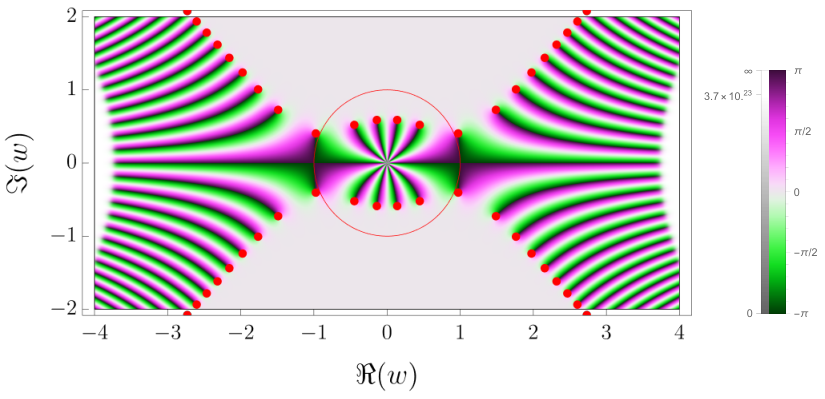
Let us first study the function (which is a function of ). It has an infinity of zeroes in the complex plane
(they are represented by red dots in the Figures S4, S5, S6 and S7). To obtain their analytical expressions one writes
(S183)
Taking the power and multiplying by we obtain
(S184)
with and for any , we denote .
Now, since the solution of is , where is any of the branches of
the Lambert function with corless1996lambertw, we obtain that the zeroes of can be written as , where
(S185)
We have further defined
(S186)
Below we will always denote . Finally, let us note that
has a pole of order at the origin .
Figure S4: Representation of , i.e. the phase (shown by a color code)
of the rescaled function for and
in the complex plane. The plot was made using the ComplexPlot function of Mathematica with the GreenPinkTones color function.
The red dots represent the zeroes of the function and we have represented the circle of radius which
corresponds to contour (equal to the circle mentionned in the text. The black lines
can be interpreted as the positions of branch cuts in and we see that the contour does not cross them.Figure S5: Same as Fig. S4 with . Note the
four zeroes on the real axis which correspond to (in the order of increasing real parts)
to . This feature happens
for any . These zeroes are related to
the soliton rapidities, for the solution where solitons are present, see discussion in the text.
As these zeroes get closer and merge pairwise.
For the zeroes go along a curve in the plane, see Fig. S6.
Figure S6: Same as Fig. S4 with . The horizontal branch cuts originating from the origin and from infinity have merged at and expand in lower and upper half planes. We will not study in details
the case here since we do not need it for our large deviation problem.
Figure S7: Same as Fig. S4 with . As discussed in the text, in the special
case of large positive , one needs to deform the circular contour (in an obvious way) to avoid the branch cuts in .
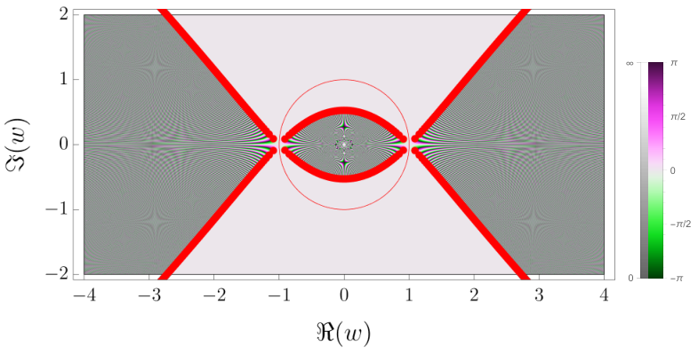
Figure S8: Same as Fig. S4 with and .
Figure S9: Same as Fig. S4 with and .
Now recall that we expect to be analytic inside a contour (we will
call the interior of ) and to be analytic outside the contour
in the complementary domain . In practice, in most cases
one can take the contour to be a circle of radius ,
in which case is analytic for for
and is analytic for .
In some special case however (see below) we will need to deform the circle.
From the knowledge of the zeroes of , one can then determine the solution for and . There are two types of solutions:
Solution without soliton.
Let us first assume that has no zeroes for
and that has no zeroes for , or more generally for
and respectively.
From Cauchy’s theorem, and taking into account that both functions are even functions of
one has, for
(S187)
where in the second equality we have closed the contour at infinity (assuming that
goes to unity for ). Similarly one has, for
(S188)
Subtracting these equations, we find
(S189)
where everywhere we denote
(S190)
Note that since the number of zeroes of is infinite,
has zeroes inside the contour (i.e. in ), and
has an infinite number of zeroes outside the contour (i.e. in ).
The positions of these zeroes are shown as red dots in the Figures S4, S5, S6, S7 for .
These zeroes lead to branch cuts in the
function as can be seen on these figures. We have checked
that for , which is the region
that we need for our large deviation problem,
there is a choice of the contour so that no branch cut is
crossed when integrating over the
contour . There exists a threshold value
such that for the contour can be
chosen to be the circle of radius (represented
as a circle of radius unity in the rescaled variables in the figures).
For the contour can be chosen as a deformed circle
as can be seen from Fig. S7. The value
increases very fast with and corresponds to
the first time that a zero initially inside the circle hits the circle
as increases
(we did not attempt to find its analytical value, except for
where one has .
Finally, we also plotted the zeroes for in Figs. S8 and S9.
One can see that they fall on some limit curves that we did not attempt to describe or interpret.
Solution with a soliton. From the considerations discussed in the text, we know that there should be
another branch of solutions with solitons. Indeed for
there are two pairs of real zeroes of ,
(we recall that
we denote ) as can be seen in Fig. S5. Furthermore one has
and
. Thus in the interval
one can consider a solution such that
has two zeroes at
inside the -circle,
and has two zeroes at ,
outside the -circle. It is then natural to redefine
(S191)
Since the product
and also tend to one at infinity, we can apply the same
manipulations as above to and . The solution thus reads
is given as a principal value. The discussion above about the contour and branch cut applies identically.
This is quite analogous to the situation for the KPZ equation (which as we show is
reached for ) as found in krajenbrink2021inverse and confirmed by the rigorous recent work of Ref. TsaiIntegrability.
XI Calculation of the rate functions
XI.1 Values of the conserved quantities
From Section VIII we can now obtain the values taken by
the conserved quantities from the coefficients of the Laurent or Taylor series of
the scattering amplitudes. One writes
(S195)
(S196)
Recalling the definition (S190) of ,
this leads to
(S197)
(S198)
This is the result in the absence of soliton. In the presence of soliton there is an additional additive contribution
so that the values of the conserved quantities are now and
respectively, where are still given by the above expressions and, from (S193)
for
Series expansion of and cumulants of . Recall the contour representation of the -th Hermite polynomial
(S208)
where the contour encloses the origin.
Expanding the logarithm in Eq. (S205) as a series, this leads to
(S211)
where we have used the value of the Hermite polynomial of even indices at the origin
(S212)
Integrating once w.r.t we obtain
(S213)
One finds that the radius of convergence of this series in is precisely
defined above , which is consistent with the behavior of the
solutions.
Let us note that the typical value
is given by the coefficient for i.e. one has
(S214)
which coincides with the prediction from the Poisson kernel. More generally, since is the generating function of the
cumulants of , from its definition (S49), one has, to leading order in
(S215)
which implies that
(S216)
In particular the variance reads
(S217)
One can easily check the first two cumulants for .
Let us recall that . For one
has
and one finds
and in agreement with the above formula.
Finally, one can obtain the cumulants of from the derivatives of the rate function
(see e.g. in (krajenbrink2017exact, Sec. 4.2.5 of the Supp. Mat.)).
Here they scale as . The variance reads
(S218)
XI.3 Rate function : second branch, with a soliton
In presence of a soliton, from (S201) we see that the value of the conserved quantity
is changed by
(S219)
On the second (solitonic) branch, the rate function thus becomes
with
(S220)
where we have replaced by
their explicit values from (S185).
Upon integration one finds that
(S221)
which vanishes as it should at which is the point where solitons are spontaneously generated.
XII Convergence to KPZ
XII.1 Convergence of the large deviation rate function
We will now show that the large deviation result for the OY polymer
(S222)
converges to the similar result for the short time KPZ equation as under
a proper rescaling. We will consider successively the right hand side of (S222) (the large deviation form)
and its left hand side (the observable) and show that each side converges to the corresponding
one for the KPZ equation.
Consider the r.h.s. of (S222). Let us consider first the main branch. One recalls that
(S223)
Note that since grows very fast with we need only to
consider the case where the contour is a circle.
We parametrize the circle of radius as , and for
large we expand around as
where we recall that . We can then make the connection on the right hand
side of the equation (S222) with the known result for the short time KPZ
equation with droplet initial conditions le2016exact; krajenbrink2021inverse as
(S227)
with the identification
(S228)
Hence the "KPZ time" must be identified with the weak noise parameter .
In the case of the second (solitonic) branch we need to study the large limit of
given by Eq. (S221). We recall the expansions of the Lambert functions for and
Now we need to consider the left hand side of (S222), and identify the observables in the two models.
For this we will use the result from Ref. (BorodinMacdo, Section 5.4.1 Formula (5.9)), which
we first state in the notations of that paper. There is it shown that the OY
partition sum denoted there converges for to the
continuum directed polymer partition sum (in the notations of BorodinMacdo) as
(S234)
On the other hand the partition sums defined here are related to those in that paper via
(S235)
We can choose , and we obtain the convergence
(S236)
where we have identified , i.e. we set .
Let us now recall that in our previous work krajenbrink2021inverse we define the
continuum directed polymer partition as the solution of the SHE
(S237)
where is the standard (unit variance) space-time white noise. Comparing with
Ref. BorodinMacdo we see that we need to write
where we recall that and that for the droplet solution
of the KPZ solution we have defined in Ref. krajenbrink2021inverse.
XII.2 Convergence of the dynamical system (10) to the nonlinear Schrodinger equation
In this Section, we investigate how to take the limit of the WNT of the O’Connell-Yor polymer (10) to the WNT equations of the Kardar-Parisi-Zhang equation directly. To this aim, we define a scaling variable , which can be interpreted as a lattice length, and and introduce the rescaled space and time as
(S241)
We then define the partition function as
(S242)
and similarly for which we relate to a response field . Definition (S242) implies the differential relations
(S243)
where we have assumed a small expansion in the last two equations. In order to keep only one dominant term in the expansion, we consider the following combination
(S244)
Upon convergence, we find that the original dynamical system (10) reads at leading order
(S245)
To obtain a final system independent on , we finally rescale the fields and as
(S246)
to obtain the system studied in the context of the WNT of the KPZ equation krajenbrink2021inverse.
XII.3 Convergence of the Lax pair (13) to the Lax pair of the nonlinear Schrodinger equation
Recalling the driftless Lax pair for the O’Connell-Yor system
(S247)
From (S244) and (S243) we observe that in order to study the convergence of the Lax pair, we need to consider the following combination
(S248)
as well as the first order in of the equations and where is the identity matrix. Indeed, in the continuum we want to transform the Lax pair (S247)
into a continuous version
(S249)
Equation (S244) together with Eq. (S248) provides a convergence to the operator which in terms of the continuous Lax matrices (S249) reads .
To study the convergence of the Lax pair, we choose the following scaling at leading order (see also (S243))
(S250)
Under this scaling, a straightforward replacement gives
(S251)
where
(S252)
(S253)
(S254)
We recognize in Eqs. (S252)-(S253) the matrices and of the continuous nonlinear Schrodinger equation obtained in the weak noise theory of the KPZ equation krajenbrink2021inverse. In particular we see the convergence
(S255)
as expected. This concludes the convergence of the Lax pairs of the discrete problem towards the continuous problem.
XIII Triangular representation of the solution to the Lax problem
Here we set and the drifts and we recall the asymptotics
(S256)
and
(S257)
and
(S258)
We have that and are analytic inside the circle
and that and are analytic outside of the circle .
(for simplicity we consider the case but the same manipulations extent to
, the contour being a deformed circle).
One introduces the triangular representations
(S259)
(S260)
The goal is to find the values of the first coefficients in the triangular representation.
Let us recall the Lax matrix where we took the drifts equal to 0.
(S261)
XIII.1 Triangular decomposition of
Injecting into one finds the recursion relations for
(S262)
(S263)
(S264)
In particular, this implies using
(S265)
where comes from the asymptotics at large . Using one has
(S266)
After further examination for all one obtains
(S267)
where all constants are determined by the asymptotic condition. We summarize our findings with the following expansion as well as Table 1
(S268)
index
Table 1: Summary of the results for and
XIII.2 Triangular decomposition of
Injecting into one finds the recursion relations for
(S269)
In particular, this implies using
(S270)
With we further obtain the cancellation of all odd terms in the triangular decomposition. Hence we obtain the following result
We also give for completeness the results for and although
we will not use them below. Injecting into one finds the asymptotic expansion
(S272)
XIII.4 Triangular decomposition of
Injecting into one finds the asymptotic expansion
(S273)
XIII.5 Additional series expansion for the Lax problem
As in Ref. merola1994novel we provide an additional discrete integral representation of the solutions to the Lax problem. Grouping the solution of the Lax problem into a matrix , we first define a rescaled matrix so that
(S274)
whose evolution and asymptotic value are given by
(S275)
Rewriting the matrix using a telescopic form and using Eq. (S275), we first obtain that
(S276)
Going back to the space, we have
(S277)
Hence we can obtain the recursion for and by inspection of the columns as
(S278)
and
(S279)
Since and are linear combinations of and , we further obtain that
(S280)
and
(S281)
Note that to have only higher order terms in the right hand side of Eq. (S280), i.e. with , it is possible to rewrite the series as
(S282)
These series representations have been used in Ref. merola1994novel to obtain analyticity results on the solution to the Lax problem. Note further that we also have the matrix factorisation .
(S283)
XIV Gelfand-Levitan-Marchenko equations
XIV.1 Notations and intermediate objects
To obtain the explicit solutions as a function of the scattering data, one needs to obtain the Gelfand-Levitan-Marchenko equations of the problem. To this aim, we start by rewriting the linear relation between and and we further insert the triangular representation of and obtained in Eqs. (S259)–(S260).
(S284)
The properties we will require are that
•
, and are analytic inside the circle ,
•
, and are analytic outside of the circle .
The analyticity properties of the various function will be used to proceed to a contour integration of Eq. (S284) using that
1.
For a function analytic inside the circle of radius , we have that
(S285)
2.
For a function analytic outside the circle of radius , we have that
(S286)
where denotes the Heaviside function. Furthermore, we use a contour integral representation of the Kronecker delta function
(S287)
We define the Fourier transform on the circle of the reflection coefficients. If the scattering data do not have any zero, it reads
(S288)
In the case of the presence of soliton, i.e. the scattering data having zeroes as in the current problem, we first proceed to the replacement
(S289)
If the scattering data have simple zeroes, e.g. and , then the expressions of and are modified to take into account the respective poles as
(S290)
where the notation stands for .
Inserting the precise value of the scattering data, i.e.
(S291)
we then obtain in the absence of soliton
(S292)
and in the presence of solitons
(S293)
Remark XIV.1.
Note that the two Fourier transforms verify the discrete linear evolution equations
(S294)
XIV.2 Derivation of the Gelfand-Levitan-Marchenko equations
First equation
We start by considering the first equation of (S284), multiply it by for and integrate it over .
(S295)
We first assume that we are in the case without soliton, i.e. no zero of and in their domain of analyticity. Using the rules (S285) and (S286), we obtain
Multiplying the equation by with and integrating over the circle of radius , we further obtain
(S299)
Making use of the contour integral representation of the Kronecker function (S287) and expanding the term as a series, we have
(S300)
Inserting the triangular representation of , from Eqs. (S259)-(S260) with the Fourier transform of the scattering data (S288) we obtain for all
(S301)
Choosing , this implies that
(S302)
The value of can be read in Eq. (S268) and the one of in Table 1.
Furthermore, choosing and separating the term out of the sum, we obtain the first Gelfand-Levitan-Marchenko equation as
(S303)
Second equation
We repeat the procedure to obtain the second GLM equation. To this aim, we consider the second equation of (S284), multiply it by for and integrate it over
(S304)
We first assume that we are in the case without soliton, i.e. no zero of and in their domain of analyticity. Using the rules (S285) and (S286), we obtain
(S305)
We then denote the following limit
(S306)
We now take so that
(S307)
Multiplying the equation by with and integrating over the circle of radius , we further obtain
(S308)
equivalent to
(S309)
Inserting the triangular representation of , from Eqs. (S259)-(S260) with the Fourier transform of the scattering data (S288) we obtain for all
(S310)
Choosing , this implies that
(S311)
The value of can be read from Eq. (S272) along side obtained for instance from Eq. (S193).
Furthermore, choosing and separating the term out of the sum, we obtain the second Gelfand-Levitan-Marchenko equation as
(S312)
XIV.3 Operator valued equations
The GLM equations obtained in Eqs. (S303)–(S312) involved summations over explicit indices. We rewrite in this Section these equations using operators and invert these to obtain explicitly the solution of the original system (10).
Let us define four operators indexed by with the following kernels
(S313)
for and we recall that the operators and are upper-triangular operators. Using the four kernels introduced and choosing for , we rewrite the two GLM equations (S303)–(S312) as
(S314)
These two equations suggest to define an operator product as
(S315)
and to define the left (resp. right) projectors to zero (resp. ), so that for any operator with kernel , we have
(S316)
Equipped with the operator product and the projector, we rewrite the diagonal contribution of the GLM equations, i.e. Eqs. (S302) and (S311), as
(S317)
where the diagonal value of the kernel of reads from Table 2
XIV.4 Inversion of the GLM equations and explicit expressions of
We invert the GLM equations to obtain the kernels of and solely in terms of the ones of and . This in turn is used to obtain the explicit expressions of as a function of the operators and .
Inversion of the GLM equation
In the first approach, we separate all the diagonals terms in (S319) and (S320) from the rest and respectively replace the values of or in each equation. From this, one obtains
(S321)
(S322)
where in both equations the right index of the kernels have to be strictly greater than , meaning that e.g. the operator can only be evaluated for .
As a corollary, we can multiply Eq. (S370) to the right by to evaluate the following product, useful for the diagonal contribution of the GLM equations.
(S323)
Exact solution for
We will now prove the following result
(S324)
To prove this, we will use Eqs. (S317) and (S323), indeed
(S325)
Isolating the second component of the above vector we find that
(S326)
Then isolating the first component of the above vector and using (S326) we find the desired result which is
(S327)
We present two other representations of the exact expression of which will be useful later on in Section XIV.5. Anticipating the result of Eq. (S342) stating that , we consider the finite difference of the resolvant and use the Sherman-Morrison formula
(S328)
We multiply (S328) by to the left and by to the right and obtain
(S329)
This leads to the second expression for
(S330)
A third expression can be obtained using that and the Sherman-Morrison formula
(S331)
We multiply (S331) by to the left and by to the right and obtain
(S332)
This leads to the third expression for
(S333)
Exact solution for
We continue by taking the right index of Eq. (S321) equal to .
(S334)
Isolating the second coefficient, we obtain
(S335)
which we have not been able to further simplify. Isolating the first coefficient, we obtain
(S336)
which is nontrivial from the exact expressions of obtained in Eqs. (S324)–(S335). As a consequence we have that
(S337)
where is the finite difference operator.
Additional identities
If we combine Eqs. (S335) and (S333), we further obtain that
(S338)
which is highly non-trivial from Eq. (S337). Furthermore, Eqs. (S324)–(S335) bring the expressions for and on a more symmetric setting, indeed
(S339)
XIV.5 Check of the time derivative of
In this Section, we verify by an algebraic method that indeed verifies the system of Eqs. (10). To this aim, we require three prelimiary results. From Equations (S294), we recall the time derivatives of the Fourier operators
(S340)
In particular, the combination of the two for any leads to
(S341)
which is a rank-one operator. Furthermore, from the definition of the product of the operators and from Eq. (S315), we obtain the following relation for the finite difference
(S342)
where so that the finite difference is a rank-one operator. More generally this relation remains valid for different indices
(S343)
The following derivative of the resolvant appearing in the expression for is obtained as follows
(S344)
Equipped with these results, we calculate the time derivative of
(S345)
Using that alongside the Sherman-Morrison formula on the second term of the right hand side, we obtain
(S346)
Using Eq. (S330), we recognise in the right hand side the expression of and we use Eq. (S337) to express the remaining difference as the product and obtain
(S347)
XIV.6 Discrete Fredholm framework for the solution of the non-linear system
The operator manipulations done so far can be related to a more fundamental object which is the Fredholm determinant of the defined as
(S348)
and we expect the operators to live to act on . Let us develop some algebraic framework for such object similarly to what was done in Refs. krajenbrink2020painleve; bothner2022riemann for the Fredholm determinant of products of continuous Hankel operators.
The finite difference relation (S342) implies a multiplicative recursion for the Fredholm determinant . Using the matrix determinant lemma, we have that
(S349)
This recursion can also be written backwards
(S350)
which implies the identity
(S351)
The multiplicative recursion between implies that a suitable object to study is actually the logarithm of the Fredholm determinant and thus we obtain that
(S352)
We also have from Eq. (S326) the relation between the logarithmic finite-difference of the Fredholm determinant and the variables of our problem.
(S353)
which implies that the logarithmic second-order finite-difference of the Fredholm determinant reads
(S354)
Exponentiating this identity, we obtain
(S355)
This identity is akin to one obtained in the continuous setting of the weak noise theory of KPZ (UsWNT2021, Eq. (13)). We can expect as in Refs. krajenbrink2020painleve; bothner2022riemann that a hierarchy of functions can be constructed which will verify a differential recursion. This precise recursion is left for future work. The first step towards this construction would be to study the finite difference of the resolvant of , the starting formula were presented in Section XIV.4 and we recall them here for completeness.
(S356)
and
(S357)
XV Limit to the classical Toda system
The weak noise theory of the O’Connell-Yor polymer can be seen as a generalisation of the classical Toda system toda1967vibration. This can be seen from the Lax pair of the model as in Ref. kuznetsov2000quantum but also directly from the dynamical system (10). To see this, consider the following Cole-Hopf type change of variable
(S358)
Note that the Jacobian of this change of variable is a constant. Then, the dynamics verified by the two fields is
(S359)
Rescaling , and , the action of the O’Connell-Yor polymer
(S54)
reads in terms of the new variables
(S360)
(S361)
Note that the terms proportional to and are respectively is a total derivative
and a constant, hence they do not contribute to the equations of motion.
Taking we find the classical Toda action, and the associated equations of motion (i.e. saddle point equations)
(S362)
This result brings a few comments:
1.
Since we have solved the weak noise theory of the O’Connell-Yor polymer using the discrete Fredholm determinant framework in Section XIV, our result is also extended for the Toda lattice.
2.
Note that our Lax pair formulation has allowed us to include drifts in the Toda system. It would be interesting
to understand their role in the dynamics.
3.
Finally, the Toda system has been related historically to the QR decomposition in linear algebra, see e.g. Refs. symes1982qr; deift1983ordinary. It would be extremely interesting to relate the O’Connell-Yor dynamics (10) as an extension of the flow of the QR decomposition. Furthermore, as we expect the existence of an integrable time discretisation of the O’Connell-Yor dynamics and thus of the Toda model, understanding the discrete flow could also shed some new light on linear algebra algorithms. We leave these questions open for a future work. Furthermore, the interpretation of the drifts in these algorithms have to be understood.
XVI Lax pair duality
The Lax pair we have studied so far involved a two-dimensional vector with two complementary fields. In this section for notation reasons, we will denote these components as
(S363)
We will show that the original Lax pair is dual to an infinite Lax pair, using the method of Ref. sklyanin2000backlund; kuznetsov2000quantum. To this aim, consider the following infinite vectors
(S364)
Our aim will be to show the existence of two matrices and such that
(S365)
and the existence of two matrices and ensuring the Lax evolutions
To start, we re-write the time equation of the Lax pair, i.e. as
(S367)
where is an infinite diagonal matrix with element equal to and has its element equal to .
Concerning the space equation of the Lax pair, i.e. , we first rescale the components
(S368)
the space Lax equation component by component is then
(S369)
So to define the spectral problem (S365) for we will eliminate in the second equation of (S369). We have two possibilities
1.
we can either invert the first equation of Eq. (S369) as
(S370)
in which case we obtain that
(S371)
Given the asymptotic data of the scattering problem, see Eqs. (S141)–(S142), we can choose and rewrite (S371) in matrix form as , where the matrix reads
(S372)
The last matrix in Eq. (S372) has the first upper band filled with and zeroes everywhere else. The intermediate matrix between the two diagonal matrices is lower-triangular filled with on the diagonal and everywhere below.
Let us look at the compatibility equation now by taking the time derivative of Eq. (S365)
(S373)
where we have used the second line of Eq. (S367) together with Eq. (S365).
We now need to use the inversion between and from Eq. (S370) to obtain
(S374)
where the scalar matrix is a lower-triangular matrix filled with on the diagonal and everywhere below.
(S375)
where we obtained the commutator was obtained using again Eq. (S365). This leads to the definition of the matrix as
Suppose , we then have the matrix representation where the reads
(S379)
The last matrix in (S379) is upper-triangular with the first band filled with and the rest is . The intermediate matrix between the two diagonal matrices is upper-triangular filled with on the diagonal and everywhere above. Let us look at the compatibility equation now by taking the time derivative of Eq. (S365)
(S380)
We now need to use the inversion between and from Eq. (S377) to obtain
(S381)
where the scalar matrix is upper-triangular filled with on the diagonal and everywhere above. It leads to
(S382)
from which we deduce the definition of the matrix
(S383)
Comment on the conserved quantities from the Lax duality
Since and verify the Lax equations
(S384)
It follows that their traces are conserved quantities, i.e. for any
As a final comment, let us mention that the local densities induced by the traces of the Lax matrices have recently been interpreted using random walks spohn2023hydrodynamic. Indeed, defining the local densities as
(S387)
they be expanded as follows
(S388)
and similarly for . Each contribution can be seen as the weight to go from site to site and the total weight is the weight of starting from site and returning to site in steps. It would be interesting to extend this interpretation in the current context and characterise the geometry and properties of the random walk.
XVII Gauge equivalence of the Lax problem with a classical integrable implicit spin chain
XVII.1 Towards a Lax pair for a spin system
Following the construction of Ishimori ishimori1982integrable which relates the Ablowitz-Ladik system to the Haldane-Ishimori-Skylanin spin chain (an integrable version discretisation of the classical Landau-Lifschitz chain) we relate our system (10) to a semi-discrete spin model. To this aim we define a gauge transform so that
This is a priori valid for an arbitrary gauge which we now specify. Here we define as the solution of (S85) for and zero drift and for convenience we rewrite (S89) as
with
(S391)
We have that verifies the compatible system
(S392)
From the evolution of the gauge we can obtain the modified Lax pair in the gauge frame. The space Lax matrix reads
(S393)
We then decompose the as
(S394)
where is the identity matrix and is the Pauli matrix . This yields
(S395)
As in Ref. ishimori1982integrable, we interpret the last term as a spin operator and to this aim we define the spin matrix as
(S396)
to rewrite the Lax matrix in the following form
(S397)
Before investigating the second Lax matrix , let us describe a few properties of the spin matrix .
It is direct to see that
(S398)
From (S392), we see that the spin allows for different rewritings.
(S399)
The second time Lax matrix is given explicitly as
(S400)
From the right hand side of (S400), we define a second spin matrix
(S401)
which has the same properties as of (S398). Note that the gauge transformation preserved the following properties of the Lax matrices
(S402)
XVII.2 Compatibility equation and spin dynamics
The compatibility equation of the gauged Lax pair reads
(S403)
Computing explicitly this compatibility equation, we observe that in order not to have a dependency on the spectral parameter in the final equation, we are required to have the identity
(S404)
This identity is indeed true and can be computed by brute-force by expanding the spin matrices with their representations, e.g. (S396), by factorising to the left and to the right . From this identity, we deduce the evolution equation for the spin
(S405)
The spins thus carry the interpretation of a local spin current.
XVII.3 A few properties to describe the spin system
Discrete parallel frame
Following Ref. hoffmann2008discrete, it is possible to interpret the spin dynamics using a discrete regular curve so that
(S406)
The spin dynamics is equivalent to the compatible system
(S407)
Since we have from the normalisation of the spin , is said to be an arclength parametrized curve and can be interpreted as a discrete parallel frame hoffmann2008discrete.
Stereographic representation and mapping from spin matrix to spin vector
Moreover, if we define the spin matrix in its stereographic representation papanicolaou1987complete as
(S408)
then we can represent it in a spin vector form as
(S409)
where we endow the vectors with the canonical real inner product to preserve the norm . Note that since the coefficients are real, this inner product is not compact, this can be seen by removing the complex in the definition of the vector and define a signed inner product with signature . A consequence of that is that two spins can have an inner product equal to 1 without equal, e.g. if for two different vectors, then their inner product is automatically equal to 1 even if the respective coefficient is arbitrary. This problem is solved in the case of complex fields when , i.e. the coefficients are complex conjugate.
In the current context, we introduce the spin vectors to relate some conserved densities and currents of the model (10) to spin quantities as in the work of Ref. zakharov1979equivalence. For a generic traceless matrix endowed with the vector representation
(S410)
we have the identity between the signed norm and the determinant . From a direct calculation, using (10) and (S392), we have that
(S411)
Taking the determinants of these equations and using the matrix determinant - spin identity, we obtain
(S412)
These expressions are exactly the densities and currents derived in Eq. (S126).
On top on the vector norms obtained, we complement this discussion by providing a few vector inner products. Using the evolution equation for (S405) as well as (S412), this yields the following inner products
(S413)
Finally, we also have for any two spins
and therefore from Eq. (S404), we obtain
(S414)
which is also interpreted as , hence the infinitesimal variation of the spin is orthogonal to the direction of the spin, which is coherent with the conservation of the norm of the spin.
In search of a Hamiltonian
At this stage, it is natural to ask whether there exists an explicit Hamiltonian such that the spin evolution can be written as
(S415)
We do expect that the Hamiltonian matches a combination of the conserved quantities of the O’Connell-Yor polymer weak noise theory after a suitable change of variable from the fields to the spins , see notably the conserved quantities in Section VIII.3.
Since both sides of the equations in (S415) are orthogonal to , we introduce the Frenet frame which can be used to decompose the vectors in a convenient basis. This frame is described by three vectors defined as
(S416)
The relation between and is still implicit at this stage but there are instances where this is easily explicit. Indeed, in the non-interacting cases, we have that
1.
If , due to the fact that is the identity. In which case we obtain
(S417)
2.
If , due to the fact that is the identity. In which case we obtain
(S418)
These equations are reminiscent of the system (10) in the non-interacting case. More generally, we leave it as an open question to decompose the vector in the Frenet frame and find the general Hamiltonian .
Finally, the spin model related to the Ablowitz-Ladik model was recently used in Ref. angelopoulos2018invariant to investigate its invariant measures. It would be interesting to see whether some techniques of Ref. angelopoulos2018invariant extend in our context of the weak noise theory of the O’Connell-Yor polymer.
XVIII Small-time limit of the Fredholm determinant result for the O’Connell-Yor polymer
In this section we start from the formula for the generating function of , the OY partition sum studied in imamura2016determinantal which is is identical to ours if we identify . We study its weak noise limit , leading to a conjectural form for
which agrees with the one derived in the text using inverse scattering. The manipulations in this
Appendix are quite heuristic but they have the merit to show that the algebraic structure which emerges from
the Fredholm determinant is similar to the one derived in the text from first principles by the inverse scattering method. The method applied in this Appendix is similar to the one used in Ref. (krajenbrink2023crossover, Section X of the Supp.Mat) in the context of the crossover from the large deviations of the macroscopic fluctuation theory to the weak noise theory of the KPZ equation.
with a contour enclosing the origin with radius and . The measure over is and we further have the constraint that
(S421)
The identification with our variables reads
(S422)
as well as
(S423)
so that the Fredholm determinant identity yields
(S424)
To complete our identification, we further introduce the relation
(S425)
Endowed with the identification, we now transform the Fredholm identity (S424) to derive the large deviation function . The first step is the introduction of a factorization of the kernel as
(S426)
where have defined the kernels
(S427)
Introducing the identity
(S428)
which we apply using
(S429)
This allows to re-write the kernel and to factorize it as
(S430)
where we have defined
(S431)
To summarise, the Fredholm manupulations we have done lead to the factorisation
(S432)
where from the first to the second line we have used Sylvester’s identity . This last Fredholm determinant has the typical structure for which the first cumulant method, developed in KrajLedou2018; ProlhacKrajenbrink; krajenbrink2019beyond to study the relevant asymptotics (here small ), applies.
This allows to formally interpret this Fredholm as an expectation value of a determinantal point process which correlations are controlled by the kernel . Hence
(S433)
where we have introduced to interpret (S433) as a linear statistics of the point process over the observable
(S434)
The first cumulant approximation applied to the expectation value (S433) asserts (KrajLedou2018, Section 6) that as some parameter goes to infinity (here it will be , see below),
we expect the point process to self-average, i.e.
(S435)
The quantity of interest only involves the diagonal part of the kernel and we have to evaluate
(S436)
taking into account that the measure on the variables is . Since , we can proceed to an integration by part with respect to the integration variable to obtain
(S437)
The function denotes the dilogarithm.
As a summary, after replacing the variable by the identification (S425), we obtain that
(S438)
and upon taking in the kernel, we have
(S439)
from the first to the second line, we have shifted the variable to absorb the additional factors in the dilogarithm. We further perform the change of variable
(S440)
and subsequently drop the tilde. Upon this change, the integral reads
(S441)
which we formally write in the following form
(S442)
Since the parameter is taken to be small, it is natural to introduce the function to obtain a rate function. Its expression reads
(S443)
We now evaluate the two integrals in using the saddle point method controlled by the rate .
From the asymptotics of the function
(S444)
alongside the expression one obtains in the limit
(S445)
At leading order, we re-write
(S446)
and obtain the rate function as
(S447)
Its derivative reads
(S448)
The saddle point equation is therefore
(S449)
At the saddle point for and the subdominant terms as well as the
constants compensates between the two integrals in (S442) and we have the following estimate
(S450)
so that
(S451)
To make this saddle point easily attainable, one way is to deform the integration contour of which is not anymore but the image of (S449) as varies along , which we call . We have also assumed that the integration contour of could be deformed to be folded around .
It is possible to further simplify the estimate of the first cumulant in (S451) by proceeding to a change of variable using the saddle point equation . The Jacobian of this change of variable reads
(S452)
To summarize, the first cumulant of the Fredholm determinant reads in the small -limit
(S453)
and our calculation have given us the following large deviation principle
(S454)
where the final large deviation function reads
(S455)
This agrees with the result of the main text (28) using the inverse scattering method.
XIX The Lambert W function
We introduce the Lambert function corless1996lambertw which we use extensively throughout this work. Consider the function defined on by , the function is composed of all inverse branches of so that . It does have two real branches, and defined respectively on and . On their respective domains, is strictly increasing and is strictly decreasing. By differentiation
of , one obtains a differential equation valid for all branches of
(S456)
Concerning their asymptotics, behaves logarithmically for large argument and is linear for small argument . behaves logarithmically for small argument . Both branches join smoothly at the point and have the value . These remarks are summarized on Fig. S10. More details on the
other branches, for integer , can be found in corless1996lambertw.
Figure S10: The Lambert function . The dashed red line corresponds to the branch whereas the blue line corresponds to the branch .