Global stabilization of a Sterile Insect Technique model
by feedback laws
Abstract
This work concerns feedback global stabilization of the sterile insect technique dynamics. The Sterile Insect Technique (SIT) is presently one of the most ecological methods for controlling insect pests responsible for crop destruction and disease transmission worldwide.
This technique consists in releasing sterile males among the insect pest population, the aim being to reduce fertility and, consequently, reduce significantly the wild insect population after a few generations.
In this work, we study the global stabilization of a pest population at extinction equilibrium by the SIT method and construct explicit feedback laws that stabilize the model. Numerical simulations show the efficiency of our feedback laws.
To the memory of Andrea Bacciotti, a wonderful person,
a leader in the field of control theory.
Keywords: Sterile Insect Technique, Pest control, Dynamical control system, Feedback design, Backstepping feedback, Lyapunov global stabilization, Mosquito population control, Vector borne disease.
1 Introduction
Mosquitoes are known to transmit a variety of diseases such as malaria, dengue, yellow fever, Zika virus and many others. These diseases are responsible for a significant number of deaths worldwide. According to the World Health Organization (WHO), the number of malaria cases worldwide in 2022 was estimated at 249 million in 85 endemic countries and territories, an increase of 5 million compared to 2021. The estimated number of deaths in 2022 is 608,000 (see [26]). Dengue and Zika virus, also transmitted by mosquitoes, are estimated to cause hundreds of thousands of cases and thousands of deaths each year. In 2023, there was an unexpected increase in dengue cases, resulting in an all-time high of more than five million cases and more than 5,000 dengue-related deaths reported in more than 80 countries/territories and five WHO regions: Africa, the Americas, South-East Asia, the Western Pacific, and the Eastern Mediterranean (see [32]).
Although there are many effective vector control measures for malaria and arboviroses, some of them can have negative impact on the environment and may result in ecological damage. For example, insecticide spraying can have unintended effects on non-target organisms, including beneficial insects such as bees and butterflies [28, 25]. In addition, repeated use of insecticides often leads to the development of resistance in mosquito populations [27].
The sterile insect technique (SIT) has been proposed as an alternative tool for reducing mosquito populations. The technique involves sterilizing male mosquitoes (frequently this is done using ionizing radiation) and then releasing them into the wild to mate with wild females. This strategy was initially applied successfully (since the 1950s) to nearly eradicate the screw-worm fly in North America. Since then, this technique has also been used for different agricultural pests and disease vectors [14, 17, 31].
One advantage of using such a technique is that it only targets the desired species and also significantly reduces the impact on the ecosystem. This is why this technique is increasingly used for the control of insect pests and insect disease vectors. Some previous works have considered applications of feedback controls to SIT: impulsive feedback controls for a 3-D model [15, 16], optimal controls for a 2-D model [6] and even optimal impulsive controls for an epidemic model for a vector borne disease in the human population [5].
For the sake of simplicity, in this paper we chose to focus our presentation on the particular and important case of mosquito population control but many of the results presented can be extended to the use of SIT for the control of other pests.
In order to determine the appropriate releases of sterile males to approach the extinction equilibrium of the population, we use mathematical control theory which provides the necessary tools for constructing such a control. Our work involves building this feedback law starting from the model proposed in [30] without the Allee effect. Our theoretical results are illustrated with numerical simulations. Moreover, in section 4 we do a comparative study between the different feedback laws.
Remark 1.1.
While we were finishing writing this work, we learned that the reduced system (system of two ODE studied in [6]) was also recently studied by A. Cristofaro and L. Rossi in [21]. In particular, they were able to construct a feedback law leading to global stabilization of the extinction equilibrium in this setting using a backstepping approach.
2 Mathematical modeling of mosquito population dynamics
2.1 Mathematical modeling of wild mosquito population dynamics
The life cycle of mosquitoes has many stages but we will consider a simplified model where we just separate an aquatic and an adult phase. The aquatic phase includes egg, larva and pupa stages. After the pupa stage, adult mosquitoes emerge and it is in the adult phase that mosquitoes reproduce and only female mosquitoes bite.
As a matter of fact, in order to lay their eggs, female mosquitoes need not only to be fertilized by males but also to have a blood meal. Thus, every 4-5 days, they will take a blood meal (that can sometimes involve biting several victims) and lay 100 to 150 eggs in different places (10 to 15 per place). An adult mosquito usually lives for 2 to 4 weeks. The mathematical model we present takes into account the two phases: the aquatic phase that we denote by and the adult phase that we split into two sub-compartments, males, , and females, . We consider the dynamics presented in [30]. Based on this model and neglecting the Allee effect (i.e. taking in system (2) of [30], which is the less favorable case for stabilizing the zero solution), we obtain the system
| (2.1) | ||||
| (2.2) | ||||
| (2.3) |
where,
- •
is the mosquito density in aquatic phase at time ;
- •
is the wild adult male density at time ;
- •
is the density of adult females at time ; we have supposed that all females are immediately fertilized in this setting and this equation is the only one that changes when we add the sterile males in which case only a fraction of the females will be fertilized;
- •
is the oviposition rate;
- •
are the death rates for eggs, wild adult males and fertilized females respectively;
- •
is the hatching rate for eggs;
- •
the probability that a pupa gives rise to a female, and is, therefore, the probability that it gives rise to a male. And, to simplify, we suppose females become fertilized immediately when they emerge from the pupal stage;
- •
is the environmental capacity for eggs. It can be interpreted as the maximum density of eggs that females can lay in breeding sites. Since here the larval and pupal compartments are not present, it is as if represents all the aquatic compartments, in which case in this term represents a logistic law’s carrying capacity for the aquatic phase that also includes the effects of competition between larvae. It has the dimensions of a spatial density.
We set and . The model (2.1)-(2.3) can be written in the form
| (2.4) |
where represents the right hand side of (2.1)-(2.3). The map is continuously differentiable on . Note that if and , then, for every , is defined and belongs to . Setting the right hand side of (2.1)-(2.3) to zero we obtain the extinction equilibrium and the non-trivial equilibrium given by
| (2.5) | ||||
| (2.6) | ||||
| (2.7) |
where
| (2.8) |
Note that if and only if . Let us now recall some definitions connected to the stability of an equilibrium.
Definition 2.1.
Let be an equilibrium (of (2.4)). The equilibrium is stable in if, for every , there exists a such that
| (2.9) |
The equilibrium is unstable in if it is not stable in . It is an attractor in if there exists such that, for every initial data in satisfying , as . It is a global attractor in if, for every initial data in , as . It is locally asymptotically stable in if it is both stable and an attractor in . Finally, it is globally asymptotically stable in if it is both stable and a global attractor in .
The Jacobian of system (2.1)-(2.3) computed at the extinction equilibrium is
| (2.10) |
Its characteristic polynomial is
| (2.11) |
Its roots are and the roots of equation
| (2.12) |
If , all eigenvalues of are either negative or have negative real parts, which implies that 0 is locally asymptotically stable. If the eigenvalues of are , , and . If , the eigenvalues of are all real, one is strictly positive, two are strictly negative.
The global stability properties of the extinction equilibrium are described in terms of the basic offspring number of the population. This is a key parameter in the theory of population dynamics. Depending on its value, more precisely if and only if , there exists a non-trivial equilibrium point (see [33, 6]). The essential properties of the model (2.1)-(2.3) are summarized in the following theorem similar to [10, Theorem 7] and [11, Theorem 1].
Theorem 2.1.
The following properties hold.
- (P.1)
If , then is a globally asymptotically stable equilibrium in for (2.4);
- (P.2)
If , then the system has two equilibria 0 and in , where is stable with basin of attraction and 0 is unstable in with the non negative being a stable manifold.
Proof.
Let us first prove (P.1). We could proceed as in the proof of [10, Theorem 7 (i)] or [11, 1) in Theorem 1] which are based on properties of monotone operators. We propose a different approach, now based on Lyapunov functions. Let be a solution of (2.4) defined at time and such that . One has
| (2.13) |
which implies that
| (2.14) |
| (2.15) |
Inequality (2.14) shows that is a stable equilibrium in for (2.4) if is a stable equilibrium in for the subsystem in :
| (2.16) | ||||
| (2.17) |
Inequality (2.15) shows that is a global attractor in for (2.4) if is a global attractor in for the subsystem (2.16)-(2.17) in .
Hence, in order to prove (P.1), it suffices to check that is globally asymptotically stable in for the system (2.16)-(2.17). To prove this last statement, let us consider the Lyapunov function , , defined by
| (2.18) |
Then,
| (2.19) | |||
| (2.20) | |||
| (2.21) |
The time-derivative of along the trajectories of (2.16)-(2.17) is
| (2.22) |
Let us now assume that
| (2.23) |
From (2.22) and (2.23) one gets
| (2.24) |
We are going to conclude by using the LaSalle invariance principle. Let us assume that we have a trajectory of (2.16)-(2.17) such that
| (2.25) |
Then, using (2.24),
| (2.26) |
Let us assume that there exists such that
| (2.27) |
Then there exists such that
| (2.28) |
which, together with (2.26), implies that
| (2.29) |
Differentiating (2.29) with respect to time and using (2.17) we get
| (2.30) |
in contradiction with (2.28). Hence
| (2.31) |
Differentiating (2.31) with respect to time and using (2.16) we get that
| (2.32) |
With the LaSalle invariance principle, this concludes the proof of (P.1).
Remark 2.1.
Let us now prove (P.2). We first note that one has the following lemma, whose proof is obvious and is omitted.
Lemma 2.1.
Let be a solution of (2.4) defined at time and such that . Then it is defined on . Moreover, if , then there exists one and only one time such that and one has
| (2.33) |
Thanks to this lemma we are allowed to assume that , which we do from now on. We then follow the proof of [10, Theorem 7 (ii)]. To prove the stability and basin of attraction of the non-trivial equilibrium we use [29, Theorem 2.2 in Chapter 2]. This theorem applies to strongly monotone systems. The Jacobian (2.10) associated with (2.4) is not irreducible. Let us consider the subsystem for and , that is (2.16)-(2.17), which defines a dynamical system on . Its Jacobian
| (2.34) |
is irreducible. Considering the usual coordinate-wise comparison and applying [29, Theorem 2.2 in Chapter 2] to the two dimensional interval
| (2.35) |
it follows that every solution starting in this interval, excluding the end points and , converges to one of the end points.
The Jacobian at is
| (2.36) |
Its characteristic equation is
| (2.37) |
whose discriminant is
| (2.38) |
The eigenvalues are
| (2.39) | |||
| (2.40) |
Therefore, since , and so 0 is unstable. Since is a Metzler matrix, it has a strictly positive eigenvector corresponding to the positive eigenvalue , which is
| (2.41) |
Moreover, the eigenvector corresponding to the negative eigenvalue is
| (2.42) |
which has two components with opposite signs and is thus biologically meaningless. Hence, no solution converges to except the trivial solution which is identically equal to . Therefore, every nontrivial solution converges to . The implication for the three dimensional system (2.1)-(2.3) is that all solutions starting in the interval excluding the -axis, converge to .
Using the same argument as in [11], any solution starting at a point larger than converges to . Since any point in can be placed between a point below , but not on the -axis, and a point above , every solution starting in converges to . The monotone convergence of the solutions initiated below and above implies the stability of as well. This concludes the proof of (P.2) and of Theorem 2.1. ∎
2.2 SIT model in mosquito population dynamics
The SIT model obtained neglecting the Allee effect from the one presented in [30] is
| (2.43) | ||||
| (2.44) | ||||
| (2.45) | ||||
| (2.46) |
where is the density of sterilized adult males, is the death rate of sterilized adults, is the control which is the density of sterile males released at time , and accounts for the fact that females may have a preference for fertile males. Then, the probability that a female mates with a fertile male is . From now on we assume that
| (2.47) |
which is a biologically relevant assumption (and even if this were not so, the sterile males would have a competitive advantage due to a higher longevity that would make SIT more efficient).
Let . When applying a feedback law , the closed-loop system is the system
| (2.48) |
where
| (2.49) |
Concerning the regularity of the feedback law, we always assume that
| (2.50) |
Note that, even if is of class , the map is not continuous and one needs to specify the definition of the solutions for the closed-loop system (2.48). Carathéodory solutions seem to be natural candidates. Roughly speaking, Carathéodory solutions are absolutely continuous curves that satisfy the integral version of the differential equation. These solutions are indeed useful in other contexts. However, if they can lead to robustness for small errors on the control, as shown in [9], they may not be robust with respect to arbitrary small measurement errors on the state, which is crucial for the application. To have a robustness with respect to arbitrary small measurement errors on the state, as shown in [24] (see also [20]), the good definition of the solutions for the closed-loop system (2.48) are the Filippov solutions, i.e. the solution of
| (2.51) |
where
- •
is the unit ball of ;
- •
for a set , is the smaller closed convex set containing ;
- •
is the set of subsets of of zero Lebesgue measure.
- •
Let us recall that , (where is an interval of ) is a solution of (2.51) if and is such that
| (2.52) |
For references about Filippov solutions, let us mention, in particular, [22, 23] and [13, Chapter 1]. For the definition of stability, global attractor and asymptotic stability, we use again Definition 2.1 (with instead of ) and take now into account all the solutions in the Filippov sense in this definition. The motivation for using Filippov solutions is given in [20, Proposition 1.4]. The global asymptotic stability in this Filippov sense implies the existence of a Lyapunov function [18]; see also [20, Lemma 2.2]. This automatically gives some robustness properties with respect to (small) perturbations (including small measurement errors on the state), which is precisely the goal of feedback laws. In fact, for many feedback laws constructed in this article, an explicit Lyapunov function will be given, which allows to quantify this robustness.
Let us emphasize that in our case the Filippov solutions of our closed-loop system have the following properties
| (2.53) | |||
| (2.54) |
From now on, the solutions of the closed-loop systems considered in this article are always the Filippov solutions.
Proposition 2.1 (See[6]: Stability properties of the system (2.43)-(2.46)).
Let us assume that
| (2.55) |
Then the following properties hold.
- 1.
If we have two equilibria:
- •
the extinction equilibrium 0, where ,which is linearly unstable;
- •
the persistence equilibrium
(2.56) (2.57) (2.58) (2.59) which is locally asymptotically stable.
- •
- 2.
Concerning the global asymptotic stability of 0 for the system (2.43)-(2.46) in , using a Lyapunov approach, one can get the following theorem.
Proof.
Let . We are going to conclude by applying Lyapunov’s second theorem. To do so, a candidate Lyapunov function is , , defined by
| (2.62) |
Note that, since ,
| (2.63) | |||
| (2.64) |
Moreover, along the trajectories of (2.43)-(2.46),
| (2.65) |
From (2.62) and (2.65), one gets
| (2.66) |
with
| (2.67) |
Let us point out that, for every solution of the closed-loop system (2.43)-(2.46) defined at time and such that ,
| (2.68) | |||
| (2.69) |
From (2.53), (2.54), (2.63), (2.66), (2.68) and (2.69), one has, for every solution of the closed-loop system (2.43)-(2.46) defined at time and such that ,
| (2.70) |
which, together with (2.63) and (2.64), concludes the proof of Theorem 2.2 (and even shows the global exponential stability and provides an estimate on the exponential decay rate given by (2.67)). ∎
3 Global stabilization by feedback of the extinction equilibrium
3.1 Backstepping feedback
For the backstepping method, the control system has the following structure:
| (3.1) | ||||
| (3.2) |
where the state is and the control is . The key and classical theorem for backstepping is the following one (see, for instance, [12, Theorem 19.2, page 110] or [19, Theorem 12.24, page 334]).
Theorem 3.1.
Assume that and are of class and that for the control system
| (3.3) |
where the state is and the control is , can be globally asymptotically stabilized by means of a feedback law of class . Then, for the control system (3.1)-(3.2), can be globally asymptotically stabilized by means of a continuous feedback law .
Let . One way to rewrite the dynamics (2.43)-(2.46) is
| (3.4) |
where
As is not of class and the feedback law has to be non-negative, we cannot directly apply the backstepping theorem. However, to build the feedback law we use the classical Lyapunov approach of the proof of Theorem 3.1 (see, for example, [19, pages 334–335]) allowing us to select an appropriate control. Unfortunately, the control that we get with this approach is not positive all the time. To get around this, using the same Lyapunov function, we propose a new feedback law that is non-negative, decreases the Lyapunov function and leads to global asymptotic stability of the extinction equilibrium.
First, consider the control system with the state being and the control being . We assume that is of the form and study the closed-loop system
| (3.8) |
We have
| (3.9) |
It is a smooth dynamical system on which is also a positively invariant set for this dynamical system.
Setting the right hand side of (3.9) to zero we obtain the equilibrium and the non-trivial equilibrium given by
| (3.10) | ||||
| (3.11) | ||||
| (3.12) |
where the offspring number is now
| (3.13) |
Note that if , is the only equilibrium point of the system in .
Our next proposition shows that the feedback law stabilizes our control system if .
Proposition 3.1.
Proof.
We apply Lyapunov’s second theorem. To do so, we define
| (3.15) | ||||
Let us define
| (3.22) |
and, for for and (the latter having dimension of a rate ) chosen in , the map , by
| (3.23) |
| (3.24) |
Finally, let us define the feedback law , , by
| (3.25) |
Note that , which is Lebesgue measurable, is not continuous in . However
| (3.26) |
Property (3.26) is important for the applications since it implies that the density of sterile males released is going to be small when the state is close to 0. For instance, this is essential to reduce the number of mosquitoes necessary for a long term intervention and also to allow using the sterile mosquitoes which are no longer needed in an area where the population is already close to zero, to intervene in other zones.
This is in contrast with the constant control in Proposition 2.1. Property (3.26) also implies that , which allows to consider Filippov solutions for the closed-loop system, i.e. the system (2.43)-(2.46) with the feedback law (3.25).
Theorem 3.2.
Proof.
Let us define by
| (3.27) | |||
| (3.28) |
We have
| (3.29) | |||
| (3.30) | |||
| (3.31) | |||
| (3.32) |
From now on, and until the end of this proof, we assume that is in and until (3.43) below we further assume that
| (3.33) |
One has
| (3.34) |
| (3.35) | |||||
| (3.36) |
We take as given by (3.25).
Therefore, in case
| (3.37) |
we have
which, together with (3.36), leads to
| (3.38) |
Otherwise, i.e. if (3.37) does not hold,
| (3.39) |
so, by (3.25),
| (3.40) |
We consider two cases:
Case 1:
Using (3.36), (3.39) and (3.40)
| (3.41) |
Case 2:
Using once more (3.36) and (3.40)
| (3.42) |
Using (2.47)
which, together with (3.42), implies that
| (3.43) |
To summarize, using (3.21), (3.38), (3.41) and (3.43), one gets the existence of , independent of , such that
| (3.44) |
Since one still has (2.53), (2.54), (2.68) and (2.69) (for ), this proves Theorem 3.2 as in the proof of Theorem 2.2 (and, again, even gives the global exponential stability and provides an estimate on the exponential decay rate). ∎
Remark 3.1.
It is important to note that the backstepping feedback control (3.25) does not depend on the environmental capacity , which is can also be an interesting feature for the field applications.
3.1.1 Numerical simulations
The numerical simulations of the dynamics when applying the feedback (3.25) are shown in figure 3.1. The parameters we use are set in table 1. The condition (3.14) gives . We fix and we consider the persistence equilibrium as initial condition. That gives and . We take , and .
| Parameter | Name | Value interval | Chosen value | Unity |
|---|---|---|---|---|
| Effective fecundity | 7.46-14.85 | 10 | Day-1 | |
| Mating competitiveness of sterilized males | 0-1 | 1 | - | |
| Hatching parameter | 0.005-0.25 | 0.05 | Day-1 | |
| Mosquitoes in aquatic phase death rate | 0.023-0.046 | 0.03 | Day-1 | |
| Female death rate | 0.033-0.046 | 0.04 | Day-1 | |
| Males death rate | 0.077-0.139 | 0.1 | Day-1 | |
| Sterilized male death rate | 0.12 | Day-1 | ||
| Probability of emergence | 0.49 |
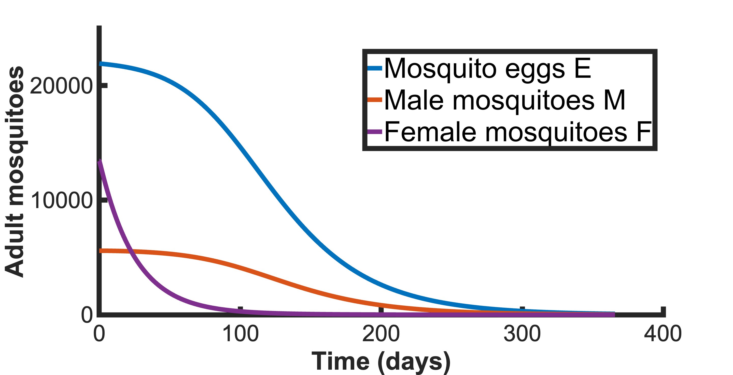
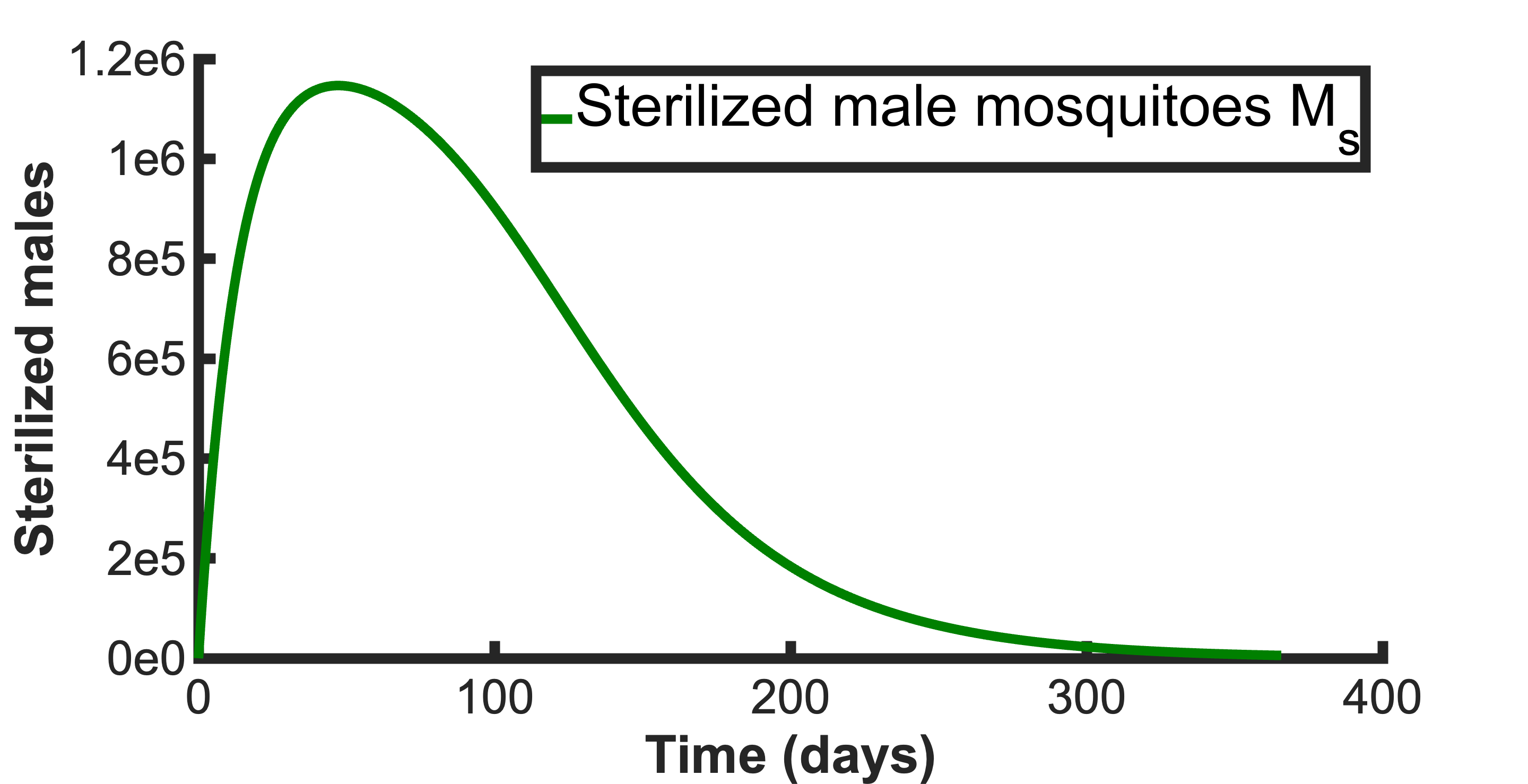
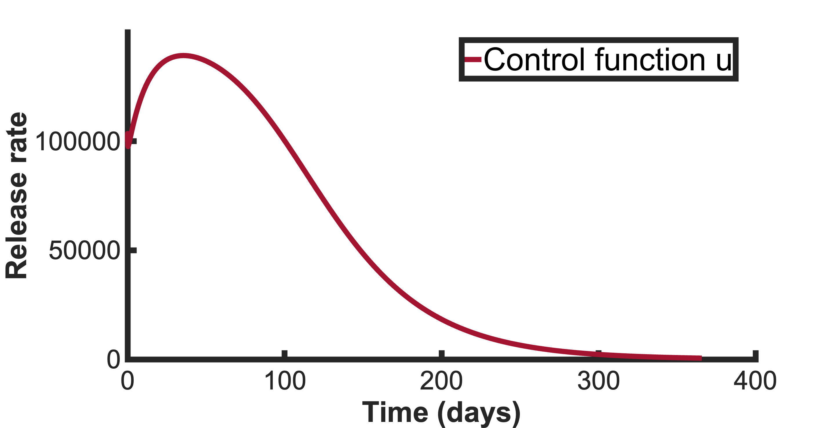
Figure 3.1.
(a): Plot of and when applying the feedback (3.25), the initial condition being the the persistence equilibrium. (b): Plot of . (c): Plot of the feedback control function .
In this case, with days,
| (3.45) |
3.1.2 Robustness test
To analyze the robustness of our feedback law we use the following protocol: the feedback law is given by (3.25) with fixed values of the parameters corresponding to the ones chosen in table 1, but for computing the real dynamics of the system (2.48) we consider simultaneous random perturbations of the system parameters with the following distribution
| (3.46) | ||||
where is the uniform distribution on interval .
Figure 3.2 shows simulations with random initial conditions in .
![[Uncaptioned image]](2307.00846v2/EMFrobust.png)
We observe that the feedback (3.25) is robust: it still stabilizes the dynamics at extinction equilibrium if the changes in the parameters are not too large.
To apply the feedback (3.25) we must estimate the number of male and female mosquitoes and the number of eggs. Some techniques used to measure these parameters are CDC light traps and BG-Sentinel traps. Based on mosquito behavior, such as their attraction to pheromones or light, these traps use different attractants, such as light, CO2, or human odor, to capture them. To estimate the population size and the ratio of sterile to fertile mosquitoes a common technique is to do Mark-release-recapture (MRR) studies. It consists in marking a subset of the released mosquitoes with a unique identifier and releasing then into the wild. By comparing the number of marked and unmarked mosquitoes captured in the traps, an estimate of the total population size and the ratio of sterile to fertile mosquitoes can be obtained. Some oviposition traps may be used to capture and count the number of eggs laid by female mosquitoes. To take into account the possible difficulty and cost of measuring all the variables ( and )in the field, in the next sections (3.2 and 3.3), we propose feedback laws depending on less variables.
3.2 Feedback laws depending only on the total number of male mosquitoes
Some recent adult traps are able to count automatically the number of male mosquitoes that are captured and, even in a more classic setting, there exist traps that use synthetic versions of female insect pheromones to attract and capture male insects. This kind of traps placed at different locations in the field, allow us to determine of the target pest population. Our aim in this section is to build a feedback linearly depending on . Consider the closed-loop system
| (3.47) |
where
| (3.48) |
| (3.49) |
and is a fixed real number. Throughout all this section 3.2, we assume that (2.55) holds and that
| (3.50) |
The offspring number related to this system is
| (3.51) |
3.2.1 Equilibria of the closed-loop system
Equilibria of the SIT model (3.47) are obtained by solving the system
| (3.52) |
We get either the extinction equilibrium 0, i.e.
| (3.53) |
or
| (3.54) |
Let us assume in the sequel that
| (3.55) |
Using (3.54) and (3.55), one gets and therefore the equilibrium given by (3.54) is not relevant. In conclusion the closed-loop system (3.47) has one and only one equilibrium which is the extinction equilibrium 0. It is therefore tempting to raise the following conjecture (compare with Theorem 2.1).
Conjecture 3.1.
The extinction equilibrium 0 is globally asymptotically stable in for the closed-loop system (3.47).
We have not been able to prove this conjecture. However,
- 1.
- 2.
In section 3.2.4, we provide numerical evidence for this conjecture.
3.2.2 Invariant set of the closed-loop system
From (2.55), (3.50), and (3.55), one gets
| (3.56) |
Let us define, with ,
| (3.57) | |||
| (3.58) |
and, for ,
| (3.59) |
One has the following theorem.
Theorem 3.3.
Remark 3.2.
Proof of Theorem 3.3.
Let us first study the case where one starts with : we consider the Filippov solution(s) to the Cauchy problem
| (3.63) |
where is such that
| (3.64) |
From (3.48), (3.49), and (3.63), one gets
| (3.65) | |||
| (3.66) |
In particular, for every , . It remains to check that
| (3.67) |
From (3.66), one has
| (3.68) |
From (3.61) one has
| (3.69) |
Property (3.67) readily follows from (3.64), (3.68) and (3.69).
Let us now deal with the case where . Note that, for , this implies that
| (3.70) |
Until the end of the proof of Theorem 3.3 we assume that and is such that (3.70) holds.
Let be defined by
| (3.71) |
Its time derivative along the solution of the closed-loop system (3.47) is
| (3.72) |
For a set , let us denote by its boundary in . On ,
. Hence
| (3.73) |
In particular, using (3.60),
| (3.74) |
3.2.3 Global asymptotic stability result
Let
| (3.83) | |||
| (3.84) |
Let us recall that, by (3.62), , which clearly satisfies (3.60), satisfies also (3.61). In particular, by Theorem 3.3, is positively invariant for the closed-loop system (3.47). The main result of this section is the following theorem.
Theorem 3.4.
Proof.
The first step of the proof is the following lemma which shows that Theorem 3.4 holds with replaced by provided that (3.60) is a strict inequality and that (3.61) holds.
Lemma 3.1.
To prove this lemma we use a Lyapunov approach. Our Lyapunov function is , ,
| (3.86) |
where is a constant which will be chosen later on. One has
| (3.87) | |||
| (3.88) | |||
| (3.89) |
Let us assume for the time being that
| (3.90) |
Then, the time derivative of along the solution of the closed-loop system (3.47) is
| (3.91) |
In particular,
| (3.92) |
Let us now point out that (3.85) implies that
| (3.93) |
From (3.92) and (3.93) one gets that for small enough there exists independent of such that
| (3.94) |
It remains to remove assumption (3.90). Let
be a Filippov solution of the closed loop system for the initial condition . We observe that if , then implies that , from which one gets that for every . Hence (3.94) holds for every . While, if , then for every . In particular, one still has (3.92) and therefore (3.94) for every . Hence,
| (3.95) |
which, together with (3.88) and (3.89), concludes the proof of Lemma 3.1.
Let us now deduce from Lemma 3.1 that
| 0 is a global attractor for the closed-loop system (3.47) in . | (3.96) |
Let be a Filippov solution of the closed-loop system (3.47) for the initial condition . If then one has (3.65) and (3.66) which leads to as (note that, by (3.62), ). Let be defined by
| (3.97) |
Note that, if for some , then there exists satisfying (3.61) and (3.85) such that . By Lemma 3.1 one then has as . If there is no such then
| (3.98) |
From (3.77) with , (3.83), (3.97), and (3.98), one gets that
| (3.99) |
which together with (3.82) implies that
| (3.100) |
Since , (3.57) and (3.100) imply that
| (3.101) |
Then, if for some , , one has , which, as already pointed out above, implies that as . It remains to handle the case where
| (3.102) |
In particular, since , one has, using (3.58),
| (3.103) |
Then, differentiating (3.101) with respect to time and using (3.47) and (3.49), one gets
| (3.104) |
which leads to a contradiction with (3.102). This concludes the proof of (3.96).
In order to conclude the proof of Theorem 3.4 it just remains to check that
| 0 is stable for the closed-loop system (3.47) in . | (3.105) |
For that, let , , be defined by
| (3.106) |
which corresponds to the definition of given in (3.86) with . Let
be a Filippov solution of the closed loop system for the initial condition . As above, we may restrict our attention to the case where
| (3.107) |
Let us recall that since , (3.58), and (3.107) imply that
| (3.108) |
Then, can be differentiated with respect to time and one has, by (3.92) with and , and (3.83),
| (3.109) |
which shows that
| (3.110) |
It remains to estimate and . Using and (3.59), one already has
| (3.111) |
Using (3.47), (3.48), (3.49), (3.62), (3.83), and (3.111), one has
| (3.112) |
In particular, using also (3.111),
| (3.113) |
This concludes the proof of (3.105) and, therefore, of Theorem 3.4. ∎
3.2.4 Numerical simulations
In this section, we will show numerical simulations of the dynamics when we apply feedback (3.48). We fix . We now compute condition (3.56) according to the parameter set in the table 1. This gives . We take . The following figures show the evolution of the states when condition (3.56) holds.


Remark 3.3.
We observe that the convergence time of the states and is longer than when we applied the backstepping feedback control (3.25). In this case, with days,
| (3.114) |
We take several initial conditions randomly and plot the resulting dynamics in figure 3.4,
![[Uncaptioned image]](2307.00846v2/EMF100Ms.png)
Figure 3.4.
Plot of when applying the feedback (3.48) with several randomly chosen initial conditions .
3.2.5 Robustness test
To analyze the robustness of our feedback against variations of the parameters, we carry out some variation of the parameters (new values) in table 2. The results are summarized in table 2.
| Old parameters | New Parameters | Simulation |
| • = 0.05 • = 0.03 • = 0.04 • = 0.1 • = 0.12 • =8 | • = 0.08 • = 0.046 • = 0.033 • = 0.12 • = 0.139 • =11 |
•
Plot of and
![[Uncaptioned image]](2307.00846v2/robalphaMs.png)
|
We observe that very small perturbations of the parameters destabilize the origin.
3.3 Feedback laws depending only on wild male mosquitoes
In the application of the technique it might also be possible to estimate only fertile males. For instance, in MRR experiments, sterile mosquitoes are identified by the presence of a marker, such as a dye or a fluorescent protein, which has been applied before their release (although, at present, it is not always easy to do this for all the mosquitoes released in field interventions). Nevertheless, since the technology is evolving very fast, it is possible that it can become standard practice in the near future (for instance, we recall that PCR analysis of the captured mosquitoes is already currently used thanks to genetic bar-coding). Thus, it is interesting to set up the mathematical techniques to deal with this situation. Therefore, we consider in this section the case where the feedback depends only on the state . Consider the closed-loop system
| (3.115) |
where
| (3.116) |
and
| (3.117) |
The offspring number related to this system is
| (3.118) |
We assume that
| (3.119) |
Note that this inequality is equivalent to
| (3.120) |
Let us point out that the closed-loop system (3.115) is exactly the closed-loop system (3.47) if one performs the following change of variables (with natural notations):
| (3.121) |
Hence Theorem 3.3 and Theorem 3.4 lead to the following theorem.
Theorem 3.5.
3.3.1 Numerical simulations
In this section, we present the numerical evolution of the states when we apply feedback (3.48). We fix as initial condition and We now compute condition (3.56) according to the parameters set in table 1. This gives . We take for the simulation .
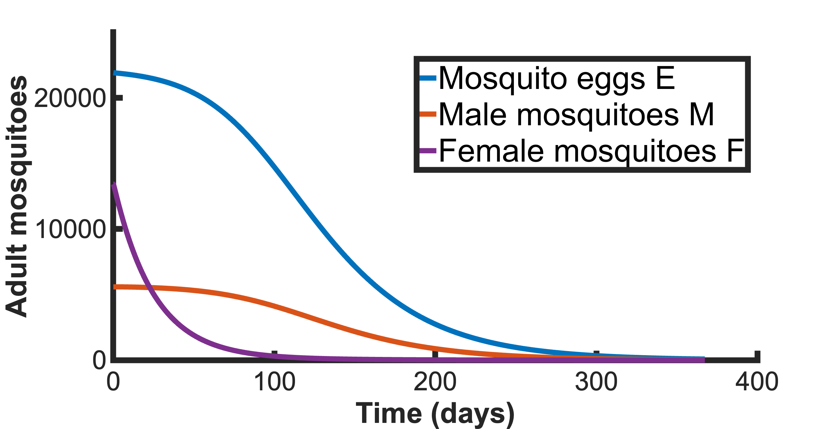
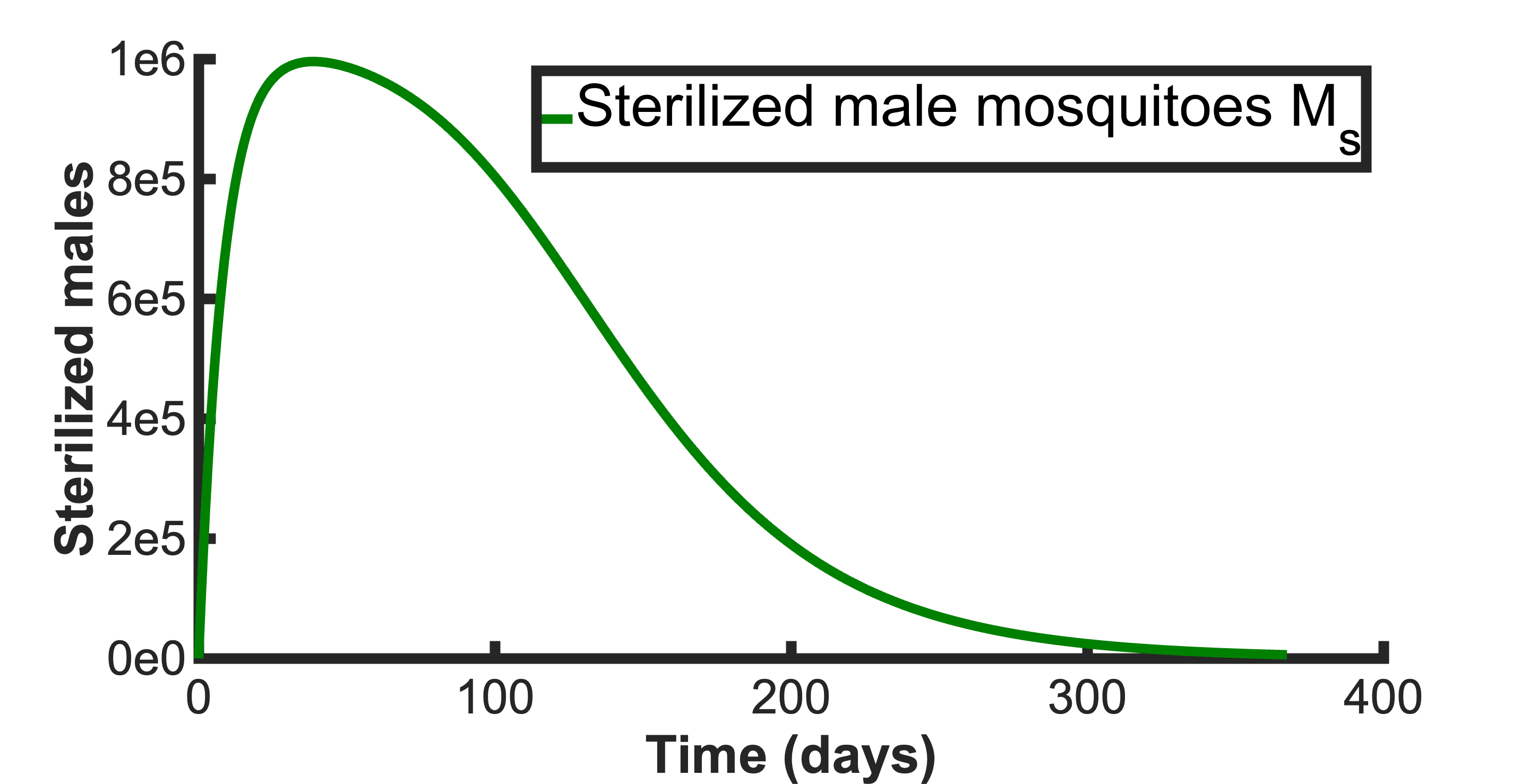

Remark 3.4.
Notice that with days,
| (3.122) |
In figure 3.6 we take several initial conditions randomly for .
![[Uncaptioned image]](2307.00846v2/plusEMFlambda.png)
Figure 3.6.
Plot of when applying the feedback (3.116) with several randomly chosen initial conditions .
3.3.2 Robustness test
We test the robustness using the same protocol as in section 3.1.2. Figure 3.7 shows the results for 200 randomly chosen initial conditions in .
![[Uncaptioned image]](2307.00846v2/RobustEMFlambda.png)
Figure 3.7.
Robustness test when applying the feedback law (3.116) with .
We observe that feedback (3.116) is robust with respect to changes of parameters: for rather large perturbations on the parameters it stills globally stabilizes the dynamics at the extinction equilibrium.
4 Comparison of the feedback laws
In this section, we use numerical simulations to carry out a comparative study of the feedback control (3.25) and (3.116). We consider that the environmental capacity and that the initial condition is the persistence equilibrium. Our comparison criteria are the intervention time and the control cost obtained when applying the different feedback laws. The results are presented in Tables 3 and 4 where the intervention is presented until . is used to regulate the control feedback law (3.116) while the regulation parameters for the backstepping control are , and .
Table 3 shows the intervention time and control cost for different values of . In table 4, we fix and present the results obtained for different values of . Note that since and are regulatory values for control (3.25), a study can be carried out to find their optimal values in order to have a better value of the control (3.25) presented here.
| Intervention | ||||||||||||||
|---|---|---|---|---|---|---|---|---|---|---|---|---|---|---|
| 9.06 | 10 | 11 | 12 | 13 | 14 | 15 | 16 | 17 | 18 | 19 | 20 | 21 | 22 | |
| (Day-1) | 667 | 477 | 424 | 390 | 367 | 350 | 336 | 326 | 318 | 311 | 305 | 300 | 295 | 291 |
| 8.24e6 | 8.61e6 | 9.14e6 | 9.72e6 | 1.03e7 | 1.09e7 | 1.16e7 | 1.22e7 | 1.29e7 | 1.35e7 | 1.42e7 | 1.48e7 | 1.55e7 | 1.61e7 | |
| Intervention | |||||||||||||
|---|---|---|---|---|---|---|---|---|---|---|---|---|---|
| 100 | 110 | 120 | 130 | 140 | 150 | 160 | 170 | 180 | 190 | 200 | 210 | 220 | |
| (Day-1) | 484 | 445 | 417 | 396 | 379 | 366 | 355 | 345 | 338 | 331 | 325 | 319 | 315 |
| 6.49e6 | 6.74e6 | 7.02e6 | 7.33e6 | 7.65e6 | 7.98e6 | 8.32e6 | 8.67e6 | 9.02e6 | 9.38e6 | 9.74e6 | 1.01e7 | 1.04e7 | |
Remark 4.1.
For 10 and for 170 we obtain nearly the same control cost for the two different interventions, but the convergence time for the intervention is smaller. This means that for the same control cost, the intervention saves time.
For and , the two interventions give approximately the same convergence time, but the cost is least for the intervention. We conclude that for the same convergence times, the intervention offers a better cost.
In conclusion, we note that thanks to the and control parameters, despite the non-linearity of the backstepping control, it offers a better result in terms of both convergence time and control cost.
5 Conclusion
We have built feedback laws that stabilize the SIT dynamical model and have studied their robustness with respect to changes of parameters. We study three types of feedback laws:
For the first one we were able to prove the global asymptotic stability. Based on the analysis done in section 4 we see that this feedback law gives a better result in terms of both convergence time and control cost. However, it depends on three variables and which may be difficult to measure in the field.
For the second one, we proved the global asymptotic stability only in a certain invariant set . We conjecture that this feedback gives global stability and we show numerical evidence for this conjecture (see figure 3.4). The advantage of this feedback law is that it depends only on the total number of male mosquitoes which is a natural quantity to measure in the field.
However, this feedback law has an important drawback due to the narrow interval allowed for the gain of the feedback in (3.56). This might pose a problem for the robustness of this method relative to the variations of the biological parameters.
For the third one, we proved the global asymptotic stability only in a certain invariant set . We also conjecture that this feedback gives global stability and we show numerical evidence for this conjecture (see figure 3.6). The main difference w.r.t. the previous feedback law is that now the method is robust w.r.t. variations of the biological parameters. However, the drawback in this case is that should be harder to measure in the field.
Changes of the environment in time, and in particular seasons (both in tropical and in temperate climates), are known to have a big impact on the mosquito populations and it will thus be important to take them into account in our future work.
Also in our work, we did not consider the pest population’s spatial distribution. This has again an impact in practical terms and has been considered in several mathematical works and, in particular, those concerning invasion wave blocking [7], the rolling carpet strategy [8] or a space dependent mosquito carrying capacity [4]. In our future works, we will construct observers that can estimate the state from easily measurable variables (after this paper was submitted a first observer construction was done in [1]) and we will also integrate the spatial aspect in this dynamical model. After the first version of this paper, other output feedback results using reinforcement learning were obtained in [2, 3].
As stated in the introduction, although the paper is mostly written for the specific case of mosquitoes, our results can be extended to the case of other pests for which the Sterile Insect Technique is pertinent.
Acknowledgements
The authors would like to thank Hervé Bossin and René Gato for the very interesting discussions that helped them identify feedback laws that can be useful for field applications and to be aware of their limitations. We hope that our future collaborations will allow us to develop and apply the ideas put forward in this work in field interventions and learn from the results to be able to improve our strategies.
References
- [1] Kala Agbo bidi. Feedback stabilization and observer design for sterile insect technique models. Mathematical Biosciences and Engineering, 21(6):6263–6288, 2024.
- [2] Kala Agbo bidi, Jean-Michel Coron, Amaury Hayat, and Nathan Lichtlé. Reinforcement learning in control theory: A new approach to mathematical problem solving. In The 3rd Workshop on Mathematical Reasoning and AI at NeurIPS’23, 2023.
- [3] Kala Agbo bidi, Jean-Michel Coron, Amaury Hayat, and Nathan Lichtlé. Reinforcement learning in control theory: A new approach to mathematical problem solving. 2023.
- [4] Luís Almeida, Jesús Bellver, Gwenaël Peltier, and Nicolas Vauchelet. Optimal strategies for mosquitoes replacement strategy: influence of the carrying capacity on spatial releases. preprint hal-04196465, September 2023.
- [5] Luís Almeida, Jesus Bellver Arnau, Yannick Privat, and Carlota Rebelo. Vector-borne disease outbreak control via instant vector releases. ,to appear in J. Math. Biol., 2024.
- [6] Luís Almeida, Michel Duprez, Yannick Privat, and Nicolas Vauchelet. Optimal control strategies for the sterile mosquitoes technique. Journal of Differential Equations, 311:229–266, 2022.
- [7] Luís Almeida, Jorge Estrada, and Nicolas Vauchelet. Wave blocking in a bistable system by local introduction of a population: application to sterile insect techniques on mosquito populations. Math. Model. Nat. Phenom., 17:22, 2022. Publisher: EDP Sciences.
- [8] Luís Almeida, Alexis Léculier, and Nicolas Vauchelet. Analysis of the rolling carpet strategy to eradicate an invasive species. SIAM J. Math. Anal., 55(1):275–309, 2023.
- [9] Fabio Ancona and Alberto Bressan. Flow stability of patchy vector fields and robust feedback stabilization. SIAM J. Control Optim., 41(5):1455–1476, 2002.
- [10] Roumen Anguelov, Yves Dumont, and Jean Lubuma. Mathematical modeling of sterile insect technology for control of anopheles mosquito. Computers & Mathematics with Applications, 64(3):374–389, 2012.
- [11] Roumen Anguelov, Yves Dumont, and Ivric Valaire Yatat Djeumen. Sustainable vector/pest control using the permanent sterile insect technique. Mathematical Methods in the Applied Sciences, 43(18):10391–10412, 2020.
- [12] Andrea Bacciotti. Local stabilizability of nonlinear control systems, volume 8 of Series on Advances in Mathematics for Applied Sciences. World Scientific Publishing Co., Inc., River Edge, NJ, 1992.
- [13] Andrea Bacciotti and Lionel Rosier. Liapunov functions and stability in control theory. Communications and Control Engineering Series. Springer-Verlag, Berlin, second edition, 2005.
- [14] H Barclay and M Mackauer. The sterile insect release method for pest control: a density-dependent model. Environmental Entomology, 9(6):810–817, 1980.
- [15] Pierre-Alexandre Bliman, Daiver Cardona-Salgado, Yves Dumont, and Olga Vasilieva. Implementation of control strategies for sterile insect techniques. Math. Biosci., 314:43–60, 2019.
- [16] Pierre-Alexandre Bliman and Yves Dumont. Robust control strategy by the Sterile Insect Technique for reducing epidemiological risk in presence of vector migration. Math. Biosci., 350:Paper No. 108856, 23, 2022.
- [17] Kostas Bourtzis and Marc J. B. Vreysen. Sterile insect technique (sit) and its applications. Insects, 12(7), 2021.
- [18] Frank H. Clarke, Yuri S. Ledyaev, and Ronald Jay Stern, Stern. Asymptotic stability and smooth Lyapunov functions. J. Differential Equations, 149(1):69–114, 1998.
- [19] Jean-Michel Coron. Control and nonlinearity, volume 136 of Mathematical Surveys and Monographs. American Mathematical Society, Providence, RI, 2007.
- [20] Jean-Michel Coron and Lionel Rosier. A relation between continuous time-varying and discontinuous feedback stabilization. J. Math. Systems Estim. Control, 4(1):67–84, 1994.
- [21] Andrea Cristofaro and Luca Rossi. Backstepping control for the sterile mosquitoes technique: stabilization of extinction equilibrium. working paper or preprint, 2023.
- [22] Alexey Fedorovich Filippov. Differential equations with discontinuous right-hand side. Mat. Sb. (N.S.), 51 (93):99–128, 1960.
- [23] Alexey Fedorovich Filippov. Differential equations with discontinuous righthand sides, volume 18 of Mathematics and its Applications (Soviet Series). Kluwer Academic Publishers Group, Dordrecht, 1988. Translated from the Russian.
- [24] Henry Hermes. Discontinuous vector fields and feedback control. In Jake K. Hale and Joseph P. LaSalle, editors, Differential Equations and Dynamical Systems (Proc. Internat. Sympos., Mayaguez, P.R., 1965), pages 155–165. Academic Press, New York, 1967.
- [25] Rajwinder Kaur, Diksha Choudhary, Samriddhi Bali, Shubhdeep Singh Bandral, Varinder Singh, Md Altamash Ahmad, Nidhi Rani, Thakur Gurjeet Singh, and Balakumar Chandrasekaran. Pesticides: An alarming detrimental to health and environment. Science of The Total Environment, page 170113, 2024.
- [26] World Health Organization. World malaria report 2023. World Health Organization, 2023.
- [27] SHP Parakrama Karunaratne, Priyanka P De Silva, Thilini Chathurika Weeraratne, Sinnathamby Noble Surendran, et al. Insecticide resistance in mosquitoes: Development, mechanisms and monitoring. 2018.
- [28] Francisco Sánchez-Bayo. Indirect effect of pesticides on insects and other arthropods. Toxics, 9(8):177, 2021.
- [29] Hal L Smith. Monotone dynamical systems: an introduction to the theory of competitive and cooperative systems: an introduction to the theory of competitive and cooperative systems. Number 41. American Mathematical Soc., 1995.
- [30] Martin Strugarek, Hervé Bossin, and Yves Dumont. On the use of the sterile insect release technique to reduce or eliminate mosquito populations. Applied Mathematical Modelling, 68:443–470, 2019.
- [31] Marc JB Vreysen, Jorge Hendrichs, and Walther R Enkerlin. The sterile insect technique as a component of sustainable area-wide integrated pest management of selected horticultural insect pests. Journal of Fruit and Ornamental Plant Research, 14:107, 2006.
- [32] World Health Organization. Dengue and severe dengue - global update, 2023. Accessed: 2024-08-17.
- [33] HMl Yang, MDLDG Macoris, KC Galvani, MTM Andrighetti, and DMV Wanderley. Assessing the effects of temperature on the population of aedes aegypti, the vector of dengue. Epidemiology & Infection, 137(8):1188–1202, 2009.