Thermodynamic Formalism and Perturbation Formulae for Quenched Random Open Dynamical Systems
Abstract.
We develop a quenched thermodynamic formalism for open random dynamical systems generated by finitely branched, piecewise-monotone mappings of the interval.
The openness refers to the presence of holes in the interval, which terminate trajectories once they enter; the holes may also be random. Our random driving is generated by an invertible, ergodic, measure-preserving transformation on a probability space .
For each we associate a piecewise-monotone, surjective map , and a hole ; the map , the random potential , and the hole generate the corresponding open transfer operator . The paper is divided into two chapters. In the first chapter we prove, for a contracting potential, that there exists a unique random probability measure supported on the survivor set satisfying .
Correspondingly, we also prove the existence of a unique (up to scaling and modulo ) random family of functions that satisfy .
Together, these provide an ergodic random invariant measure supported on the global survivor set , while combined with the random closed conformal measure yields a random absolutely continuous conditional invariant measure (RACCIM) supported on .
Further, we prove quasi-compactness of the transfer operator cocycle generated by and exponential decay of correlations for .
The escape rates of the random closed conformal measure and the RACCIM coincide, and are given by the difference of the expected pressures for the closed and open random systems. Finally, we prove that the Hausdorff dimension of the surviving set is equal to the unique zero of the expected pressure function for almost every fiber . We provide examples, including a large class of random Lasota-Yorke maps with holes, for which the above results apply.
In the second chapter of the paper we consider quasi-compact linear operator cocycles , and their small perturbations . The operators and need not be transfer operators.
We prove an abstract -wise first-order formula for the leading Lyapunov multipliers , where quantifies the closeness of and .
We then consider the situation where is a transfer operator cocycle for a closed random map cocycle
and the perturbed transfer operators are defined by the introduction of small random holes in , creating a random open dynamical system.
We obtain a first-order perturbation formula in this setting, which reads where is the unique equivariant random measure (and equilibrium state) for the original closed random dynamics.
Our new machinery is then deployed to create a spectral approach for a quenched extreme value theory that considers random dynamics and random observations.
An extreme value law is derived using the first-order terms .
Further, in the setting of random piecewise expanding interval maps, we establish the existence of random equilibrium states and conditionally invariant measures for random open systems with small holes via a random perturbative approach, in contrast to the cone-based arguments of the first chapter.
Finally we prove quenched statistical limit theorems for random equilibrium states arising from contracting potentials.
We illustrate all of the above theory with a variety of examples.
Chapter 0 Introduction
In this paper we develop a quenched thermodynamic formalism for random open dynamical systems, and their perturbations. This work may be seen as a successor to [3], which was devoted to the construction of conformal measures and equilibrium states for random potentials associated to countably branched random maps of the unit interval. We now extend such a formalism to the more challenging setting of random open dynamical systems. A random dynamical system is qualified to be open if it contains holes which terminate trajectories once they enter. Similarly, when referring to a closed dynamical system, we mean a dynamical system (in the usual sense) without a hole in phase space. These notions of openness and closedness have nothing to do with the topological concepts of open and closed sets. Throughout the text we will refer to open and closed measures and open and closed transfer operators, by which we mean measures and transfer operators associated to the random dynamical system with or without holes, respectively. We note that our closed transfer operator does not have any relation to the notion of closed (unbounded) linear operators.
The current paper is divided into three chapters. In the first chapter, the random holes are allowed to be large ensuring that the asymptotic dynamics take place on a surviving set and the objective will be to define equilibrium states and their variational principles. A key step in this program will be the construction of (random) conditionally invariant probability measures. Moreover we will give an explicit formula for the escape rate. In the second chapter, the introduction of a decreasing family of small random holes with measure tending to zero are seen as a perturbation of a transfer operator. We will first develop a perturbation theory for (nonautonomous) cocycles of transfer operators, which we will then use to study the escape rates and recurrence to small random holes. We then use our general random perturbation theory to prove extreme value laws. Finally, in the third chapter, we present a short selection of open questions.
Summary of Chapter 1. Thermodynamic formalism for random interval maps with holes
Deterministic closed transitive dynamics with enough expansivity enjoy a “thermodynamic formalism”: the transfer operator with a sufficiently regular potential has a unique absolutely continuous invariant measure (ACIM) , absolutely continuous with respect to the conformal measure . Furthermore, arises as an equilibrium state, i.e. a maximiser of the free energy, which is a sum of the integral of the potential and the metric entropy .
Continuing with the deterministic setting, if one introduces a hole , the situation becomes considerably more complicated. In the simplest case where the potential is the usual geometric potential , because of the lack of mass conservation, one expects at best an absolutely continuous conditionally invariant measure (ACCIM) , conditioned according to survival from the infinite past, and absolute continuous with respect to the closed conformal measure . Considering the dynamics restricted to the survivor set , namely the set of points whose infinite forward trajectories remain in , there exists a unique open ACIM , supported on , absolutely continuous with respect to the open conformal measure . Early work on the existence of the ACCIM and exponential convergence of non-equilibrium densities, includes [74, 24]. The paper [60] handles general potentials that are contracting [61] for the closed system, demonstrating exponential decay for . There has been further work on the Lorentz gas and billiards [28, 29], intermittent maps [30, 32], and multimodal maps [31, 33]. In the setting of diffeomorphisms with SRB measures, following the introduction of a hole, relations between escape rates and the pressures have been studied in [34].
Looking to the fractal dimension of the surviving set , the machinery of thermodynamic formalism was first employed by Bowen [15] to find the Hausdorff dimension of the limit sets of quasi-Fuchsian groups in terms of the pressure function, and then pioneered in the setting of open dynamical systems in [72, 73].
In the random setting, repeated iteration of a single deterministic map is replaced with the composition of maps drawn from a collection . A driving map on a probability space creates a map cocycle . The authors recently developed a complete, quenched thermodynamic formalism for random, countably-branched, piecewise monotonic interval maps [3], enabling the treatment of discontinuous, non-Markov .
There are two approaches to study random dynamical systems, annealed and quenched. In the quenched setting, which is the setting in which we work, one considers general ergodic random driving and uses a fiberwise transfer operator defined for each realization of the driving to find an -family of invariant measures. Then one seeks to prove results which hold almost surely, or for a “typical” driving realization. On the other hand, in the annealed setting, one considers i.i.d. random dynamics (see Remark 0.1.1 for details) and uses the annealed (-averaged) transfer operator to find an annealed invariant measure. In the setting of i.i.d. random driving, the annealed invariant measure is the marginal of the quenched random invariant measure, see [1, 2.1.8 Theorem]. Thus, the quenched approach covers a broader class of driving mechanisms, and when the annealed approach is also available, the quenched approach provides information about specific random trajectories, as opposed to information about the averaged behaviour from the annealed perspective.
The situation of random open dynamics is relatively untouched. For a single piecewise expanding map with holes randomly chosen in an i.i.d. fashion, [11] consider escape rates for the annealed transfer operator in the small hole limit (the Lebesgue measure of the goes to zero). In a similar setting, now assuming to be Markov and considering non-vanishing holes, [10] show existence of equilibrium states, again for the annealed transfer operator. For the first time in [46] the authors consider escape rates for quenched random open interval maps where they are able to show that the escape rate is bounded above by the Lyapunov exponent of a Perron-Frobenius cocycle. In [7], the authors consider random, full-branched interval maps with negative Schwarzian derivative. The maps are allowed to have critical points, but the partition of monotonicity and holes, made up of finitely many open intervals, are fixed and non-random. In this setting the existence of a unique invariant random probability measure is proven as well as a formula for the Hausdorff dimension of the surviving set. In our current setting, we do not allow the existence of critical points, however our maps may have non-full branches, and our partitions of monotonicity as well as our holes are allowed to vary randomly from fiber to fiber.
Sequential systems with holes have been considered in [47], where a cocycle of open maps is generated by a single orbit. The maps (which include the hole) must be chosen in a small neighborhood of a fixed map (with hole), in contrast to our setting where our cocycle may include very different maps. Moreover in [47], Lebesgue is used as a reference measure and the specific potential is used. The theory is developed for uniformly expanding maps in higher dimensions and the main goal is to establish the “conditional memory loss”, a concept analogous to exponential decay of correlations for closed dynamics.
Other related work includes [4], which considered non-transitive random interval maps with holes. In [4] we proved a complete thermodynamic formalism for random interval maps (i) containing sufficiently many full branches and (ii) random potentials satisfying a strong contracting potential assumption. In the current work we treat maps that contain no full branches and potentials that satisfy a significantly weaker contracting potential assumption at the cost of assuming the closed system satisfies a mild covering condition. This allows us to obtain results for a large class of random Lasota-Yorke maps (Section 1.15.2). Furthermore, the current work and that of [4] are complementary, and neither work generalizes the other. For example, the current work does not need a full-branch condition in order to obtain a thermodynamic formalism for systems as in Chapter 1, while [4] provides such a theory (Theorems 6.1, 6.4 and 6.6) for non-transitive maps (Example 7.5) which are not covered in this work.
In Chapter 1 of the present paper, we establish a full, quenched thermodynamic formalism for piecewise monotonic random dynamics with general potentials and general driving—the random driving can be any invertible ergodic process on . We begin with the random closed dynamics dealt with in [3]: piecewise monotonic interval maps satisfying a random covering condition; we have no Markovian assumptions, our maps may have discontinuities and may lack full branches. The number of branches of our maps need not be uniformly bounded above in and our potentials need not be uniformly bounded below or above in . To this setting we introduce random holes and formulate sufficient conditions that guarantee a random conformal measure and corresponding equivariant measure supported on the random survivor set , and a random ACCIM supported on . These augment the notion of a random contracting potential [3] with accumulation rates of contiguous “bad” intervals (with zero conformal measure), and extend similar constructions of [60] to the random situation.
To establish the existence of the family of measures , we follow the limiting functional approach of [61, 60] by defining a random functional which is a limit of ratios of transfer operators and then showing that may be identified with the open conformal measure . This technique improves on the approach of [3], which uses the Schauder-Tichonov Fixed Point Theorem to prove the existence of , by eliminating the extra steps necessary to show that the family is measurable with respect to . Several steps are needed to achieve the construction of the conformal random measures. We start in Section 1.4 by giving background material on Birkhoff cone techniques and the construction of our random cones. In Section 1.5 we develop several random Lasota-Yorke type inequalities in terms of the variation and the random functional . Section 1.6 sees the construction of a large measure set of “good” fibers for which we obtain cone invariance at a uniform time step, and in Section 1.7 we show that the remaining “bad” fibers occur infrequently and behave sufficiently well. In Section 1.8 we collect further properties of the random functional , which are then used in Section 1.9 to construct a large measure set of fibers for which we obtain cone contraction with a finite diameter image in a random time step. Using Hilbert metric contraction arguments, Section 1.10 collects together the fruits of Sections 1.6-1.9 to prove our main technical lemma (Lemma 1.10.1), which is then used to (i) obtain the existence of a random density , (ii) prove the existence of a unique non-atomic random conformal measure , and (iii) a random -invariant measure which is absolutely continuous with respect to . All these facts are collected in our first result (detailed statements can be found in Corollary 1.10.6, Proposition 1.10.8, Lemma 1.10.9, Lemma 1.10.11, Proposition 1.10.14, Proposition 1.11.5, Lemma 1.11.7, and Theorem 1.13.2).
Theorem A.
Given a random open system (see Section 0.1.1) satisfying ((T1))-((T3)), ((LIP)), (GP), ((A1))-((A2)), and ((Q1))-((Q3)) (see Sections 1.1 and 1.3), the following hold.
- (1)
There exists a unique random probability measure supported in such that
for each , where
Furthermore, we have that .
- (2)
There exists a function such that and for -a.e. we have
Moreover, is unique modulo .
- (3)
The measure is a -invariant and ergodic random probability measure supported in and the unique relative equilibrium state for the potential satisfying the following variational principle:
Furthermore, for each (the set of all random -invariant Borel probability measures supported on ) different from we have that
- (4)
There exists a random conditionally invariant probability measure absolutely continuous with respect to , which is supported on , and whose disintegrations are given by
for all .
We also show that the operator cocycle is quasi-compact.
Theorem B.
With the same hypotheses as Theorem A, there exists such that for each there exists a measurable function such that for -a.e. and all we have
and
Furthermore, for all sets that are a finite union of intervals, there exists a measurable function such that we have
For the proof of Theorem B, as well as a more general statement, see Theorem 1.11.2 and Corollary 1.11.9. From quasi-compactness we easily deduce the exponential decay of correlations for the invariant measure .
Theorem C.
Theorem C (stated in more detail in Theorem 1.11.3) is proven in Section 1.11. The presence of holes leads naturally to introduce the notion of fiberwise escape rate of the measure from the holes; the definition in the random setting in given in 1.12.3. We will show that the escape rate is constant -almost everywhere and is given in terms of the closed and open expected pressures, denoted with for a given potential which are properly defined in Definition 1.12.1.
Theorem D.
With the same hypotheses as Theorem A, for -a.e. we have that
Theorem D is proven in Section 1.12. The expected pressure function is further developed and used to prove a Bowen’s formula type result for the Hausdorff dimension of the survivor set for -a.e. in Section 1.14. This requires us to introduce the bounded distortion property for a given potential, large images of the map , and large images with respect to the hole ; see Section 1.14 for the full definitions of these terms. We therefore have:
Theorem E.
With the same hypotheses as Theorem A, we additionally suppose that
and has bounded distortion. Then there exists a unique such that for all and for all .
Furthermore, if has large images and large images with respect to , then for -a.e.
where denotes the Hausdorff dimension of the set .
In Section 1.15 we apply our general theory to a large class of random -transformations with random holes as well as a general random Lasota-Yorke maps with random holes. In fact, our theory applies to all of the finitely-branched examples discussed in [3] (this includes maps which are non-uniformly expanding or have contracting branches which appear infrequently enough that we still maintain on-average expansion) when suitable conditions are put on the holes . This includes the case where is composed of finitely many intervals and the number of connected components of is -integrable with respect to .
Summary of Chapter 2. Perturbation formulae for quenched random dynamics with applications to open systems and extreme value theory
The spectral approach to studying deterministic closed dynamical systems on a phase space , centers on the analysis of a transfer operator , given by , for in a suitable Banach space and for suitable potential function . If the map is covering and the potential function is contracting in the sense of [61] (or similarly if as in [36, 35] or if as in [49, 19], or if is hyperbolic as in [53]), then one obtains the existence of an equilibrium state , with associated conformal measure , with the topological pressure and the density of equilibrium state given by the logarithm of the leading (positive) eigenvalue of and the corresponding positive eigenfunction , respectively. The map exhibits an exponential decay of correlations with respect to and .
Keller and Liverani [56] showed that the leading eigenvalue and eigenfunction of vary continuously with respect to certain small perturbations of . One example of such a perturbation is the introduction of a small hole . The set of initial conditions of trajectories that never land in is the survivor set . For small holes, specialising to Lasota-Yorke maps of the interval, Liverani and Maume-Dechamps [60] apply the perturbation theory of [56] to obtain the existence of a unique conformal measure and an absolutely continuous conditionally invariant measure , with density . The leading eigenvalue is interpretable as an escape rate, and the open system displays an exponential decay of correlations with respect to and .
To obtain finer information on the behaviour of with respect to perturbation size, particularly in the situation where the perturbation is not smooth, such as perturbations arising from the introduction of a hole, one requires some additional control on the perturbation. Keller and Liverani [57] develop abstract conditions on and its perturbations to ensure good first-order behaviour with respect to the perturbation size. Following [57], several authors [60, 40, 43, 67, 18] have used the Keller-Liverani [56] perturbation theory to obtain similar first-order behaviour of the escape rate with respect to the perturbation size for open systems in various settings.
This “linear response” of is exploited in Keller [55] to develop an elegant spectral approach to deriving an exponential extreme value law to describe likelihoods of observing extreme values from evaluating an observation function along orbits of . In particular, the limiting law of
| (0.0.1) |
where the thresholds are chosen so that for some , is shown to be exponential. The spectral approach of [55] also provides a relatively explicit expression for the limit of (0.0.1), namely
where is the extremal index.
In Chapter 2 we begin with sequential composition of linear operators , where is an invertible map on a configuration set . The driving could also be an ergodic map on a probability space . We then consider a family of perturbed cocycles , where the size of the perturbation is quantified by the value (Definition 2.1.1). Our first main result is an abstract quenched formula (Theorem 2.1.2) for the Lyapunov multipliers up to first order in the size of the perturbation of the operators . This quenched random formula generalizes the main abstract first-order formula in [57] stated in the case of a single deterministic operator .
Theorem F.
The existence of a random quenched equilibrium state, conformal measure, escape rates, and exponential decay of correlations is established in Chapter 1 for relatively large holes, generalizing the large-hole constructions of [60] for a single deterministic map to the random setting with general driving. In contrast, the focus of Chapter 2 is to establish a random quenched analogue of the results of [60], [57], and [55] discussed above. To this end, we let be the transfer operator for the open map with a hole introduced in , namely . Our second collection of main results is a quenched formula for the derivative of with respect to the sample invariant probability measure of the hole (Theorem 2.3.7), as well as a quenched formula for the derivative of the fiberwise escape rate with respect to the sample invariant probability measure of the hole (Corollary 2.3.10).
Corollary G.
To generalize to the random setting the rescaled distribution of the maxima given by (0.0.1), we now consider the real-valued random observables defined on the phase space and construct a process . We are interested in determining the limiting law of
| (0.0.3) |
where is a collection of real-valued thresholds. The sample probability measure enjoys the equivariance property however the process is not stationary in the probabilistic sense, which makes the theory slightly more difficult.
The first approach to non-stationary extreme value theory (EVT) was given under convenient assumptions, by Hüsler in [51, 52]. He was able to recover the usual extremal behaviour seen for i.i.d. or stationary sequences under Leadbetter’s conditions [58], namely (i) guaranteed mixing properties for the probability measure governing the process and (ii) that the exceedances should appear scattered through the time period under consideration. Hüsler’s results can not be applied in the dynamical systems setting because his uniform bounds on the control of the exceedances are not satisfied for deterministic, random, or sequential compositions of maps. The first contribution dealing explicitly with extreme value theory for random and sequential systems is the paper [44]; see also [42] for an application to point processes. These works were an adaptation of Leadbetter’s conditions and Hüsler’s approach: let us call them the probabilistic approach to extreme value theory, to distinguish it from the spectral and perturbative approach used in the current paper.
As in the deterministic case, in order to avoid a degenerate limit distribution, one should conveniently choose the thresholds Hüsler proved convergence to the Gumbel’s law if for some we have convergence of the sum
| (0.0.4) |
for -a.e. In our current framework we will additionally allow the positive number to be any positive random variable in . The nonstationary theory developed in [44] for quenched random processes, has the further restrictions that the observation function is fixed (-independent), and the thresholds (like the scaling ) are just real numbers, and requires the obvious restricted equivalent of (0.0.4). In our framework the observation function , the scaling , and the thresholds may all be random (but need not be). We generalize and simplify the requirement (0.0.4) to
| (0.0.5) |
where the scaling may be a random variable and the “errors” satisfy (i) a.e., and (ii) for a.e. and all sufficiently large . We provide a more detailed discussion of the relationship between the conditions (0.0.4) and (0.0.5) at the end of Section 2.4.
In summary, we derive a spectral approach for a quenched random extreme value law, where the dynamics is random, the observation functions can be random, the thresholds controlling what is an extreme value can be random, and the scalings of the likelihoods of observing extreme values can be random, all controlled by general invertible ergodic driving. Moreover, we obtain a formula for the explicit form of Gumbel law for the extreme value distribution. This leads to our main extreme value theory result (stated in detail later as Theorem 2.4.5):
Theorem H.
For a random open system (see Section 0.1.1), assuming ((C1’)), ((C2)), ((C3)), ((C4’)), ((C5’)), ((C7’)), ((C8)), and ((S)) (see Sections 2.3 and 2.4), for -a.e. one has
where and are the random conformal measure and the random invariant measure, respectively, for our random dynamics, is a random scaling function, and is an -local extremal index corresponding to the quantity given in Corollary G.
This result generalizes the spectral approach to extreme value theory in [55], for a single map , single observation function , single scaling, and single sequence of thresholds.
Given a family of random holes one can define the first (random) hitting time to a hole, starting at initial condition and random configuration :
When this family of holes shrink with increasing according to Condition ((S)) (see Section 2.4.3), Theorem H provides a description of the statistics of random hitting times, scaled by the measure of the holes (see Theorem 2.4.7).
Corollary I.
By assuming some additional uniformity in on the maps we use a recent random perturbative result [27] to obtain a complete quenched thermodynamic formalism. The following existence result extends Theorem C of [60], which concerned inserting a single small hole into the phase space of a single deterministic map , to the situation of random map cocycles with small random holes with the random process controlled by general invertible ergodic driving .
Theorem J.
Suppose that (E1)–((E9)) (see Section 2.5) hold for the random open system (see Section 0.1.1). Then for each sufficiently small there exists a unique random -invariant probability measure with . Furthermore, is the unique relative equilibrium state for the random open system and satisfies a forward and backward exponential decay of correlations. In addition, there exists a random absolutely continuous (with respect to ) conditionally invariant probability measure with and density function .
For a more explicit statement of Theorem J as well as the relevant assumptions and definitions see Section 2.5 and Theorem 2.5.12.
In Section 2.6 we prove some quenched limit theorems for closed random dynamics. These limit results are new for more general potentials and their associated equilibrium states. We use two approaches. The first is based on the perturbative technique developed in [38], which generalizes the Nagaev-Guivarc’h method to random cocycles. This technique establishes a relation between a suitable twisted operator cocycle and the distribution of the random Birkhoff sums. As a consequence, it is possible to get quenched versions of the large deviation principle, the central limit theorem, and the local central limit theorem. The second approach invokes the martingale techniques previously used in the quenched random setting in [39]. We obtain the almost sure invariance principle (ASIP) for the equivariant measure which also implies the central limit theorem and the law of iterated logarithms, a general bound for large deviations and a dynamical Borel-Cantelli lemma. In addition, using the Sprindzuk theorem we are able to obtain a quenched shrinking target result.
We conclude in Section 2.7 with several explicit examples of Theorems F–J. We start in Example 2.7.1 with the weight for a family of random maps, random scalings, and random observations with a common extremum location in phase space, which is a common fixed point of the . The special cases of a fixed map on the one hand, and a fixed scaling on the other, are also considered. The same calculations can be extended to observation functions with common extrema on a periodic orbit common to all . Next in Example 2.7.2 we consider the more difficult case where orbits are distributed according to equilibrium states of a general geometric weight , using random -maps and random observation functions with a common extremum at . Example 2.7.3 investigates a fixed map with random observation functions with extrema in a shrinking neighbourhood of a fixed point of , where the neighbourhood lacks the symmetry of Example 2.7.1. In the last example, Example 2.7.4, we again consider random maps with random observations , but now the maxima of the observations are not related to fixed or periodic points of .
Though we apply our results to the setting of random interval maps our results apply equally well to other random settings including random subshifts [13, 64], random distance expanding maps [65], random polynomial systems [17], random transcendental maps [66]. In addition, Theorem F (as well as (0.0.2) of Corollary G) applies to sequential and semi-group settings including [6, 71]. See Remark 2.5.13 for a sequential version of Theorem J.
0.1. Preliminaries on random open systems
In this section we introduce the general setup of random open systems. We begin with a probability space and an ergodic, invertible map which preserves the measure , i.e.
We will refer to the tuple as the base dynamical system. For each , let be a closed subset of a complete metrisable space such that the map
is a closed random set, i.e. is closed for each and the map is measurable (see [26]), and we consider the maps
Random iteration is given by , by which we mean the -fold composition
Thus, our random iterates are compositions which are driven by the orbits of the base dynamical system . Given a set we let
denote the inverse image of under the map for each and . Now let
and define the induced skew-product map by
Let denote the Borel -algebra of and let be the product -algebra on . Throughout the text we denote Lebesgue measure by Leb. We suppose the following:
- (M1)
The map is measurable with respect to .
Remark 0.1.1.
Throughout this manuscript we consider general ergodic driving . To consider the simpler setting of iid driving let be a finite set together with an associated probability vector . Then take to be the space of all bi-infinite sequences with symbols from , let be the left-shift map, and let be the Bernoulli measure on generated by the vector . Now for each of the symbols of , we associate a map (), and for each we denote .
Definition 0.1.2.
A measure on with respect to the product -algebra is said to be random measure relative to if it has marginal , i.e. if
The disintegrations of with respect to the partition satisfy the following properties:
- (1)
For every , the map is measurable,
- (2)
For -a.e. , the map is a Borel measure.
We say that the random measure is a random probability measure if for -a.e. the fiber measure is a probability measure. Given a set , we say that the random measure is supported in if and consequently for -a.e. . We let denote the set of all random probability measures supported in . We will frequently denote a random measure by .
The following proposition from Crauel [26], shows that a random probability measure on uniquely identifies a probability measure on .
Proposition 0.1.3 ([26], Propositions 3.3).
If is a random probability measure on , then for every bounded measurable function , the function
is measurable and
defines a probability measure on .
For functions and we let
denote the Birkhoff sums of and with respect to and respectively. We will consider a potential of the form , and for each we consider the weight whose disintegrations are given by
| (0.1.1) |
for each . We will often denote by . We assume there exists a family of Banach spaces of real-valued functions on each with such that the fiberwise (Perron-Frobenius) transfer operator given by
| (0.1.2) |
is well defined. Using induction we see that iterates of the transfer operator are given by
We let denote the space of functions such that for each and we define the global transfer operator by
for and . We assume the following measurability assumption:
- (M2)
For every measurable function , the map is measurable.
We suppose the following condition on the existence of a closed conformal measure.
- (CCM)
There exists a random probability measure and measurable functions and with such that
for all where . Furthermore, we suppose that the fiber measures are non-atomic and that with . We then define the random probability measure on by
(0.1.3)
From the definition, one can easily show that is -invariant, that is,
| (0.1.4) |
Remark 0.1.4.
Definition 0.1.5.
We are now ready to introduce holes into the closed systems.
0.1.1. Random Open Systems
We let be measurable with respect to the product -algebra on such that
For each the sets are uniquely determined by the condition that
| (0.1.5) |
Equivalently we have
where is the projection onto the second coordinate. By definition we have that the sets are -measurable. Now define
and let
Throughout the manuscript, in particular Chapter 1, we denote . For each , we define
| (0.1.6) |
to be the set of points in which survive, i.e. those points whose trajectories do not land in the holes, for iterates. We then naturally define
| (0.1.7) |
to be the set of points which will never land in a hole under iteration of the maps for any . We call the -surviving set. Note that the sets and are forward invariant satisfying the properties
| (0.1.8) |
Now for any we set
The global surviving set is defined as
for each . Then is precisely the set of points that survive under forward iteration of the skew-product map . We will assume that the fiberwise survivor sets are nonempty:
- (X)
For -a.e. we have .
As an immediate consequence of ((X)) we have that . In fact, ((X)) together with the forward invariance of the sets imply that is infinite. The following proposition presents a setting in random piecewise continuous open systems for which ((X)) holds and the survivor set is nonempty for random piecewise continuous open dynamics.
Proposition 0.1.6.
Suppose that for -a.e. there exist nonempty compact subsets such that for -a.e.
- (1)
is continuous for each ,
- (2)
, where for each .
Then for -a.e. and consequently . Furthermore, if
then for -a.e. the survivor set is uncountable.
Proof.
For each let denote the continuous map , and let denote the map . Since is compact, for each we have that is a nonempty compact subset of . Given let be an -length word with for each . Let denote the finite collection of all such words of length . Then for each and each
is compact. Furthermore, forms a decreasing sequence in . Hence, we see that
forms a decreasing sequence of compact subsets of . Thus,
as desired. The final claim follows from the ergodicity of , which ensures that for a.e. there are infinitely many such that , and the usual bijection between a point in and an infinite word in the fiberwise sequence space . ∎
Now we define the perturbed operator by
| (0.1.9) |
where for each we define , and, similarly, for each ,
Note that measurability of and condition ((M2)) imply that for every the map is also measurable. Iterates of the perturbed operator are given by
which, using induction, we may write as
We define the sets to be the support of , that is, we set
| (0.1.10) |
Note that, by definition, we have
for each , and we similarly define
From this moment on we will assume that for -a.e. we have that
| (D) |
Remark 0.1.7.
We let
| (0.1.11) |
for each . Since is the support of , using the notation of (0.1.11) we may write
More generally, we have that, for , is the support of , i.e.
| (0.1.12) |
for . Note that
| (0.1.13) |
Finally, we note that since , for each we have that
| (0.1.14) |
and
| (0.1.15) |
0.2. Simple Examples
We finish this introductory chapter by presenting a simple class of examples that satisfy our main assumptions. Consequently we have that Theorems A – D, F, H, J and Corollaries G, I hold. In particular, the examples in this section are presented purely for pedagogical purposes and do not represent the full generality of our theory. As such, we will omit technical details and proofs.
In this section we will build on the abstract framework of Sections 0.1 and 0.1.1 and consider the i.i.d. iteration of -transformations. We begin by following the i.i.d. setup of Remark 0.1.1, that is we let be a finite set together with a probability vector , and then we take , to be the shift map, and is the Bernoulli measure generated by . For each we take the fibers and we consider the measurable function where . As in Remark 0.1.1, we assume that the maps are determined by the zeroth coordinate of the bi-infinite sequence from a finite set of for . For each , we take the Banach spaces , the space of bounded variation functions, and let be given by . We consider the (closed) Perron-Frobenius operator defined by
In this case we have that the potential . Furthermore, we have that for almost every , the closed conformal measure is Lebesgue, i.e. , and it follows from [20, 3] that the assumptions ((M1)), ((M2)), and ((CCM)) are satisfied. Let be the partition of into intervals of monotonicity of the map .
Now depending on how one chooses the random holes , either large holes or holes which are sufficiently small to apply a perturbative approach, we are able to apply a different collection of our results. We will begin with the results that apply for large holes described in Chapter 1.
0.2.1. Large holes
For each , we take to be one of the intervals of monotonicity , after which we can define the open transfer operator and the surviving sets and as in Section 0.1.1. Since contains full branches outside of the hole , we have that the open transfer operator is fully supported, meaning that , which further implies that our assumption (D) holds. Furthermore, applying Proposition 0.1.6 with the sets to be these full branches outside of the hole, we see that the surviving sets are nonempty, and thus that our assumption ((X)) is satisfied. Finally, assume that
Without presenting the details, it can easily be checked that our assumptions ((T1))-((T3)), ((LIP)), (GP), ((A1))-((A2)), and ((Q1))-((Q3)) (which are presented in Chapter 1) are satisfied for the i.i.d. random -transformations described here. Thus Theorems A – D hold. Under some additional minor assumptions (bounded distortion and large images) that will be explained in Section 1.14, Theorem E can be shown to hold in this setting as well. For details and additional examples in greater generality see Section 1.15.
Now we consider examples for which the holes are chosen sufficiently small that we may take a perturbative approach as described in Chapter 2.
0.2.2. Small holes
For each fix some such that is not a point of discontinuity for the map . Let and for each take be the ball of radius centered at the point . For each define the open operators and surviving sets as in 0.1.1. As the holes are contained in single branches of monotonicity, following the same reasoning as in the setting of large holes, we again see that our assumptions (D) and ((X)) hold. It can be shown that the assumptions (E1)–((E9)) of Section 2.5 hold in this setting, and thus we have that Theorem J holds. In particular, we have that for each there exists a random conformal measure , a random invariant density , and a random invariant measure such that
for all and that there exists and such that for all
It immediately follows that our assumptions ((C1))–((C7)) of Section 2.3 hold as well as the relevant strengthenings ((C1’)), ((C4’)), ((C5’)), and ((C7’)) of Section 2.4. See Section 2.5 for further details.
In order to apply Corollary G (which is a dynamical version and corollary of the general perturbation result Theorem F), Theorem H, and Corollary I, we must check the assumptions ((C8)) and ((S)) of Sections 2.3 and 2.4 respectively. First, to satisfy ((S)) we further assume that is non-random and we take a sequence such that
for some , which can be done since (the invariant density of the random ACIM ) is uniformly (in ) bounded above and away from zero. To see that ((C8)) holds, we consider the quantity
which is a simplification of the quantity defined in (2.2.4). A simple calculation shows that for all . Thus we have only to calculate to verify ((C8)):
Thus, we have that Corollary G, Theorem H, and Corollary I hold with the random extremal index given by
For further details and more general examples see Section 2.7.
Chapter 1 Thermodynamic formalism for random interval maps with holes
In this first chapter we consider fixed random holes and the main objective will be to construct a random conformal measure and corresponding equivariant measures supported on the random survivor set The measures will be shown to be the unique relative equilibrium state for the potential . We will also get a random absolutely continuous conditionally invariant measure supported on Successively we define the escape rate of the closed conformal measure and show that it equals the difference of the expected pressures of the closed and open random systems. Finally we establish a Bowen’s like formula for the Hausdorff dimension of the survivor set for a specific potential.
1.1. Preliminaries of random interval maps with holes
We begin with a base dynamical system , i.e. the map is invertible, ergodic, and preserves the measure . For the remainder of Chapter 1 for each we take to be a compact interval in , and we consider the map such that there exists a finite partition of such that is an interval for each and
- (T1)
- (T2)
- (T3)
In addition, we will assume that
- (LIP)
The maps induce the skew product map given by
For each we consider the fiber dynamics of the maps given by the compositions
We let , for , denote the monotonicity partition of on which is given by
Given , we denote by
the inverse branch of which takes to for each . We will assume that the partitions are generating, i.e.
| (GP) |
where denotes the Borel -algebra of . Let denote the set of all bounded real-valued functions on and for each and each let
denote the variation of over . If we denote . We let
denote the set of functions of bounded variation on . For each we will set the Banach space . Let
be norms on the respective Banach spaces and . Given a function , by we mean
Definition 1.1.1.
We say that a function is random bounded if
- (1)
for each ,
- (2)
for each the function is measurable,
- (3)
the function is measurable.
Let denote the collection of all random bounded functions on .
Definition 1.1.2.
We say that a function is of random bounded variation if for each and the map is measurable. We let , which will take the place of the space from Section 0.1, denote the set of all random bounded variation functions.
As in (0.1.2), we define the (closed) transfer operator, , with respect to the potential by
For each we let and denote the respective dual spaces of and . We let denote the dual transfer operator.
Definition 1.1.3.
We will say that a measurable potential is admissible if for -a.e. we have
- (A1)
- (A2)
Remark 1.1.4.
Note that if for each then ((A2)) is immediate. Furthermore, as we also have that for -a.e. and each .
As an immediate consequence of ((A1)) we have that
| (1.1.1) |
Note that since we can write
for each we must have that . Clearly we have that the sequence is submultiplicative, i.e.
Similarly we see that the sequence is supermultiplicative. Submultiplicativity and supermultiplicativity of and together with (1.1.1) gives that
| (1.1.2) |
for each . Our assumptions ((T1)) and ((LIP)) combined with (1.1.2) implies that
| (1.1.3) |
for each . Note that, in view of (0.1.14)-(0.1.15), (1.1.2) and (1.1.3), imply that
| (1.1.4) |
The Birkhoff Ergodic Theorem then implies that the quantities in (0.1.14) and (0.1.15) are tempered, e.g.
for -a.e. and each .
In addition to the assumptions ((T1))-((T3)), ((A1)), ((A2)), (GP), and ((LIP)) above, we note that in our current setting assumption ((M1)) implies that
- (M)
The map is measurable.
Furthermore, in our current setting our assumption ((CCM)) translates to the following:
- (C)
There exists a random probability measure and measurable functions and with such that
for all . Furthermore, we suppose that the fiber measures are non-atomic and that with . The -invariant random probability measure on is given by
Remark 1.1.6.
1.1.1. Random Interval Maps with Holes
We now wish to introduce holes into the class of finite branched random weighted covering systems.
Let be measurable with respect to the product -algebra on . By definition, i.e. (0.1.5), we have that the sets are -measurable. Suppose that , that is we have
Now define
and recall from Section 0.1 that we denote
We then let
For each and we define the -surviving sets and as in (0.1.6)-(0.1.7). By definition, for each , we have that
Note, however, that these survivor sets are, in general, only forward invariant and not backward invariant. For notational convenience for any we set
For each we let , and thus for each this gives
Now define the open operator , where comes from our assumption ((C)) on the closed system, by
| (1.1.5) |
As a consequence of (1.1.5), we have that
Iterates of the open operator are given by
which, using induction, we may write in terms of the closed operator as
1.2. Random conditionally invariant probability measures
In this section we introduce the notion of a random conditionally invariant measure and give suitable conditions for their existence. As in the previous section, we consider random interval maps with holes, however we would like to point out that the definitions, results, and proofs of this section hold in the greater generality of Section 0.1. We begin with the following definition.
Definition 1.2.1.
We say that a random probability measure is a random conditionally invariant probability measure (RCIM) if
| (1.2.1) |
for all , , and all Borel sets . If a RCIM is absolutely continuous with respect to a random probability measure we call a random absolutely continuous conditionally invariant probability measure (RACCIM) with respect to .
Straight from the definition of a RCIM we make the following observations.
Observation 1.2.2.
Note that if we plug into (1.2.1) with , we have that
which immediately implies that id either or . If then we have that is supported in .
Observation 1.2.3.
Note that since
for each and we have that if is a RCIM then
for each . In particular, we have that
In light of Observation 1.2.3, given a RCIM , for each we let
Thus we have
| (1.2.2) |
We now prove a useful identity.
Lemma 1.2.4.
Given any , any , and we have that
Proof.
To prove the identity we calculate the following:
∎
The following lemma gives a useful characterization of RACCIM (with respect to ) in terms of the transfer operators .
Lemma 1.2.5.
Suppose is a random probability measure on absolutely continuous with respect to , whose disintegrations are given by
Then is a RACCIM (with respect to ) if and only if there exists such that
| (1.2.3) |
for each .
Proof.
Beginning with the “reverse” direction, we first suppose (1.2.3) holds for all . Let (Borel -algebra). Using Lemma 1.2.4 gives
| (1.2.4) |
Inserting into (1.2.4) gives
Observation 1.2.2 implies that , and thus
since . Thus, for we have
as desired.
Now to prove the opposite direction, suppose is a RACCIM. Then by the definition of a RCIM there exists such that for any we have
So we calculate
So we have
| (1.2.5) |
which completes the proof. ∎
1.3. Functionals and partitions
In this section we follow [61, 60] and introduce the random functional that we will later show is equivalent to the conformal measure for the open system. We also introduce certain refinements of the partition of monotonicity which are used to define “good” and “bad” intervals and are needed to state our main assumptions on the open system. Following the statement of our main hypotheses, we state our main results.
We begin by defining the functional by
| (1.3.1) |
We note that this limit exists as the sequence is bounded and increasing. Indeed, we have that
| (1.3.2) |
and to see that the ratio is increasing we note that
| (1.3.3) |
In particular, (1.3.2) of the above argument gives that
| (1.3.4) |
Observation 1.3.1.
One can easily check that the functional has the following properties.
- (1)
.
- (2)
is continuous with respect to the supremum norm.
- (3)
implies that .
- (4)
.
- (5)
.
- (6)
for all .
- (7)
If for some then .
Furthermore, we note that the homogeneity ((4)) and super-additivity ((5)) imply that is convex. In the sequel, we will show that is in fact linear, and can thus be associated with a unique probability measure on via the Riesz Representation Theorem.
Remark 1.3.2.
We set
| (1.3.6) |
The following propositions concern various estimates of . We begin by setting
| (1.3.7) |
Then, by the definition and (1.3.3), we have that
| (1.3.8) |
as .
Remark 1.3.3.
Proposition 1.3.4.
There exists a measurable and finite -a.e. function such that
for all . Furthermore, this implies that
| (1.3.12) |
for all .
Proof.
We proceed via contradiction, assuming that there is a sequence in such that
Let . Then, we have that
By our choice of and by the definition (0.1.10), we have that the numerator of the quantity on the right is zero, while its denominator is strictly positive. As this holds for each , this implies that for -a.e. , which contradicts (1.3.11). Thus, we are done. ∎
Remark 1.3.5.
Note that our assumption (D), that , is satisfied if for -a.e. . Moreover, this also implies that . This occurs, for example if for -a.e. there exists a full branch, i.e. there exists with , outside of the hole , in which case we would have that for -a.e. .
We now describe various partitions, which depend on the functional , that we will used to obtain a Lasota-Yorke inequality in Section 1.5. Recall that denotes the partition of monotonicity of . Now, for each and we let be the collection of all finite partitions of such that
| (1.3.13) |
for each .
Given , let be the coarsest partition amongst all those finer than and such that all elements of are either disjoint from or contained in . Now, define the following subcollections:
| (1.3.14) | ||||
| (1.3.15) | ||||
| (1.3.16) |
Remark 1.3.6.
Note that in light of (1.3.1) and (1.3.3), for every we may define the open covering time to be the least integer such that
| (1.3.17) |
which is finite since the ratio in (1.3.17) increases to . Conversely, given that the ratio in (1.3.17) is increasing by (1.3.3) we see that, for , if there exists any such that
then we must have that and equivalently .
We adapt the following definition from [60].
Definition 1.3.7.
We say that two elements are contiguous if either and are contiguous in the usual sense, i.e. they share a boundary point, or if they are separated by a connected component of .
We will consider random open systems that satisfy the following conditions.
- (Q1)
For each and we let denote the maximum number of contiguous elements of . We assume
- (Q2)
We assume that for each we have .
- (Q3)
Let
(1.3.18) We assume that, for each , .
Remark 1.3.8.
1.4. Random Birkhoff cones and Hilbert metrics
In this section we first recall the theory of convex cones first used by Birkhoff in [12], and then present the random cones on which our operator will act as a contraction. We begin with a definition.
Definition 1.4.1.
Given a vector space , we call a subset a convex cone if satisfies the following:
- (1)
,
- (2)
for all , ,
- (3)
is convex,
- (4)
for all and all with as , if for each , then .
Lemma 1.4.2 (Lemma 2.1 [61]).
The relation defined on by
is a partial order satisfying the following:
| (i) | ||||
| (ii) | ||||
| (iii) | ||||
| (iv) | ||||
| (v) |
The Hilbert metric on is given by the following definition.
Definition 1.4.3.
Define a distance by
where
Note that is a pseudo-metric as two elements in the cone may be at an infinite distance from each other. Furthermore, is a projective metric because any two proportional elements must be zero distance from each other. The next theorem, which is due to Birkhoff [12], shows that every positive linear operator that preserves the cone is a contraction provided that the diameter of the image is finite.
Theorem 1.4.4 ([12]).
Let and be vector spaces with convex cones and and a positive linear operator such that . If denotes the Hilbert metric on the cone and if
then
for all .
Note that it is not clear whether is complete. The following lemma of [61] addresses this problem by linking the metric with a suitable norm on .
Lemma 1.4.5 ([61], Lemma 2.2).
Let be a norm on such that for all if , then , and let be a homogeneous and order-preserving function, which means that for all with and all we have
Then, for all implies that
Remark 1.4.6.
Note that the choice satisfies the hypothesis, however from this moment on we shall make the choice of .
Definition 1.4.7.
For each and let
| (1.4.1) |
To see that this cone is non-empty, we note that the function for and . We also define the cone
Let and denote the Hilbert metrics induced on the respective cones and . For each , , and any set we let
and
denote the diameter of in the respective cones and with respect to the respective metrics and . The following lemma collects together the main properties of these metrics.
Lemma 1.4.8 ([61], Lemmas 4.2, 4.3, 4.5).
For the distance between is given by
If , then
| (1.4.2) |
and if , for , we then have
1.5. Lasota-Yorke inequalities
The main goal of this section is to prove a Lasota-Yorke type inequality. We adopt the strategy of [3], where we first prove a less-refined Lasota-Yorke inequality with (random) coefficients that behave in a difficult manner, and then, using the first inequality, prove a second inequality with measurable random coefficients and uniform decay on the variation as in [20].
We now prove a Lasota-Yorke type inequality following the approach of [60] utilizing the “good” and “bad” interval partitions defined in (1.3.14)-(1.3.16).
Lemma 1.5.1.
For all , all , and all there exist positive, measurable constants and such that
where
and
Proof.
Since , if , then , and thus, we have for each . Thus, considering only intervals in , we are able to write
| (1.5.1) |
where
is the inverse branch which takes to for each . Now, since
we can rewrite (1.5.1) as
| (1.5.2) |
So,
| (1.5.3) |
Now for each , using (1.3.13), we have
| (1.5.4) |
Now, using (1.5.4), we may further estimate (1.5.3) as
| (1.5.5) |
In order to investigate each of the two sums in the line above, we first note that as is finite then, by definition, there exists a constant (defined by (1.3.18)) such that
So, we may choose such that for we have
| (1.5.6) |
Note that since this ratio is increasing we have that (1.5.6) holds for all . Then for each and we have
In particular, for each , we see that
| (1.5.7) |
We are now interested in finding appropriate upper bounds for the sum
However, we must first be able to associate each of the elements of with one of the elements of . To that end, let and denote the elements of that are the furthest to the left and the right respectively. Now, enumerate each of the elements of , (clearly depends on , , and ), such that is to the right of for . Given (), with let be the union of all contiguous elements which are to the right of and also to the left of . In other words, is the union of all elements of between and . Similarly, for , we define be the union of all contiguous elements which are to the left of and also to the right of . Now, we note that our assumption ((Q1)) implies that each and () is the union of at most contiguous elements of . For let
Then for we have
| (1.5.8) |
We obtain a similar inequality for . We now consider the following two cases.
- (Case 1:)
At least one of the intervals and is an element of .
- (Case 2:)
Neither of the intervals , is an element of .
If we are in the first case, we assume without loss of generality that , and thus every element is contained in exactly one union for some for some . If and instead we have that we could simply replace with in the previous statement. In view of (1.5.8), Case 1 leads to the conclusion that
If we are instead in the second case, then for each to the left of there is exactly one , , such that . This leaves each of the elements to the right of uniquely contained in the union . Thus, Case 2 yields
Hence, either case gives that
| (1.5.9) |
Inserting (1.5.7) and (1.5.9) into (1.5.5) gives
In view of (1.3.3), taking the infimum over allows us to replace the ratio with , that is, we have
Setting
| (1.5.10) |
finishes the proof. ∎
Remark 1.5.2.
Define the random constants
| (1.5.12) |
In light of our assumption ((Q1)) on the potential and number of contiguous bad intervals, we see that exponentially quickly for each .
Proposition 1.5.3.
For each , .
Lemma 1.5.4.
For each and each we have
| (1.5.13) |
Furthermore, we have that
| (1.5.14) |
In particular, this yields
Proof.
For each with , , and we have
Taking the infimum over and letting gives
| (1.5.15) |
proving the first claim. Now to see the second claim we note that as (1.5.15) holds for all with , we must also have
| (1.5.16) |
for any and each . Proceeding via induction, using (1.5.15) as the base case, we now suppose that
| (1.5.17) |
holds for . Using (1.5.16) and (1.5.17), we see
Considering proves the final claim, and thus we are done. ∎
Define the normalized operator by
| (1.5.18) |
In light of Lemma 1.5.4, for each , , and we have that
| (1.5.19) |
Now, considering the normalized operator, we arrive at the following immediate corollary.
Corollary 1.5.5.
For all , all , and all we have
Definition 1.5.6.
Since exponentially fast by our assumption ((Q1)), we let be the minimum integer such that
| (1.5.20) |
and we define the number
| (1.5.21) |
Remark 1.5.7.
In light of Corollary 1.5.5 we may now find an appropriate upper bound for the BV norm of the normalized transfer operator.
Lemma 1.5.8.
There exists a measurable function with such that for all and each we have
| (1.5.22) |
where
Proof.
We now define the number by
| (1.5.24) |
The constants and in the Lasota-Yorke inequalities from Lemma 1.5.1 and Corollary 1.5.5 grow to infinity with , making them difficult to use. Furthermore, the rate of decay of the in Corollary 1.5.5 may depend on . To remedy these difficulties we prove another, more useful, Lasota-Yorke inequality in the style of Buzzi [20].
Proposition 1.5.9.
For each there exists a measurable, -a.e. finite function such that for -a.e. , each , and all we have
1.6. Cone invariance on good fibers
In this section we follow Buzzi’s approach [20], and describe the good behavior across a large measure set of fibers. In particular, we will show that, for sufficiently many iterates , the normalized transfer operator uniformly contracts the cone on “good” fibers for cone parameters sufficiently large. Recall that the numbers and are given by
Note that Lemma 1.5.8 and the ergodic theorem imply that
| (1.6.1) |
The following definition is adapted from [20, Definition 2.4].
Definition 1.6.1.
We will say that is a good fiber with respect to the numbers , , , and if the following hold:
| (G1) | ||||
| (G2) |
Now, we denote
| (1.6.2) |
The following lemma describes the prevalence of the good fibers as well as how to find them.
Lemma 1.6.2.
Given and , there exist parameters and (both of which depend on ) such that there is a set of good fibers with .
Proof.
We begin by letting
| (1.6.3) |
where is the -a.e. finite measurable constant coming from Proposition 1.5.9. Choose sufficiently large such that . Noting that by (1.6.2), we set and choose sufficiently large such that
Now let and define the set
Now choose such that . Set . Set
| (1.6.4) |
Then is the set of all which are good with respect to the numbers and , and . ∎
In what follows, given a value , we will consider cone parameters
| (1.6.5) |
and we set
| (1.6.6) |
The next lemma shows that the normalized operator is a contraction on the fiber cones and that the image has finite diameter.
Lemma 1.6.3.
If is good with respect to the numbers , , , and , then for each we have
1.7. Density estimates and cone invariance on bad fibers
In this section we recall the notion of “bad” fibers from [3, 20]. We show that for fibers in the small measure set,
the cone of positive functions is invariant after sufficiently many iterations for sufficiently large parameters . We accomplish this by introducing the concept of bad blocks (coating intervals), which we then show make up a relatively small portion of an orbit. As the content of this section is adapted from the closed dynamical setting of Section 7 of [3], we do not provide proofs.
Recall that is given by (1.6.6). Following Section 7 of [3], and using the same justifications therein, we define the measurable function so that
| (1.7.1) |
is the smallest integer such that for either choice of sign or we have
| (1.7.2) | ||||
| (1.7.3) |
Clearly, is a measurable function such that
| (1.7.4) | ||||
| (1.7.5) |
In particular, (1.7.4) and (1.7.5) together imply that
| (1.7.6) |
for all . Let
| (1.7.7) |
where is given by (1.6.6), and for each , given , we define the coating length as follows:
- •
if , then set ,
- •
Since by Lemma 1.5.8, we must have that
| (1.7.9) |
for all . It follows from Lemma 1.5.8 that for all we have
| (1.7.10) |
Furthermore, if it follows from (G2) that
| (1.7.11) |
The following proposition collects together some of the key properties of the coating length .
Proposition 1.7.1.
For all sufficiently small the number satisfies the following.
| (i) | ||||
| (ii) |
Remark 1.7.2.
Definition 1.7.3.
We will call a (finite) sequence of fibers a good block (originating at ) if (which implies that ). If, on the other hand, we call such a sequence a bad block, or coating interval, originating at .
For sufficiently small we have that , and so we let such that
| (1.7.12) |
We now wish to show that the normalized operator is weakly contracting (i.e. non-expanding) on the fiber cones for sufficiently large values of . We obtain this cone invariance on blocks of length , however in order to obtain cone contraction with a finite diameter image we will have to travel along several such blocks. For this reason we introduce the following notation.
Given with for each we define the length
where and for each we set . This construction is justified as we recall from Proposition 1.7.1 that for -a.e. with we have that . The next lemma was adapted from Lemma 7.5 of [3].
Lemma 1.7.4.
For sufficiently small, each , and -a.e. with we have that
| (1.7.13) |
Moreover, we have that
| (1.7.14) |
where
| (1.7.15) |
Proof.
Throughout the proof we will denote and for each . Then . Using (1.6.7) on good fibers and (1.7.10) on bad fibers, for any and we have
| (1.7.16) |
where
| (1.7.17) |
and
| (1.7.18) |
For any and we can write
The definition of , (1.7.8), then implies that
and consequently that
| (1.7.19) |
Now, using (1.7.9), (1.7.19), and (1.7.12) we see that for sufficiently small, the proportion of bad blocks is given by
| (1.7.20) |
In view of (1.7.17), using (1.7.19), (1.7.20), for any and we have
| (1.7.21) |
Now for any there must exist some and some such that . Thus, using (1.7.21) we can write
| (1.7.22) |
Now, since for all , using (1.7.18) and (1.7.19), we have that for and
| (1.7.23) |
Similarly to the reasoning used to obtain (1.7.22), for any we see that we can improve (1.7.23) so that we have
| (1.7.24) |
Thus, inserting (1.7.22) and (1.7.24) into (1.7.16) (with ) we see that
Therefore, taking sufficiently small11 1 Any such that , which implies , will suffice; see Observation 7.4 of [3] for details. in conjunction with (G1), we have that
and so we must have that
which proves the first claim. Thus, for any we have that
where we have used the fact that , and consequently we have
as desired. ∎
The next lemma shows that the total length of the bad blocks take up only a small proportion of an orbit, however before stating the result we establish the following notation. For each we let be the integer such that
| (1.7.25) |
where is a remainder term. Given , let
| (1.7.26) |
for each . Then for each we can break the -length -orbit of in into blocks of length (for ) plus some remaining block of length where plus a remainder segment of length , i.e. we can write
| (1.7.27) |
see Figure 1.1. We also note that (1.7.25) and (1.7.27) imply that
| (1.7.28) |
The proof of the following lemma is nearly identical to that of Lemma 7.6 of [3], and therefore it shall be omitted.
Lemma 1.7.5.
To end this section we note that
| (1.7.30) |
as . For the remainder of the document we will assume that is always taken sufficiently small such that the results of Section 1.7 apply.
1.8. Further properties of
In this section we prove some additional properties of the functional that will be necessary in Section 1.9 to obtain cone contraction with finite diameter. In particular, in the main result of this section, which is a version of Lemma 3.11 of [60] and dates back to [59, Lemma 3.2], we show that for a function there exists a partition element on which the function takes values at least as large as .
Now we prove the following upper and lower bounds for .
Lemma 1.8.1.
For -a.e. such that , and each we have that
Proof.
From Lemma 1.5.4 we already see that the first inequality holds. Now, fix (with ) and . To see the other inequality we first let and , then
Now taking the infimum over and letting gives
| (1.8.1) |
Now, set . Since , (1.7.14) from Lemma 1.7.4 implies that
| (1.8.2) |
where we have used the fact that which follows from (1.7.15). Combining (1.8.2) with (1.8.1), we see that
completing the proof. ∎
Lemma 1.8.2.
For each and each there exists such that for each , has the property that
Proof.
Choose such that
for each . Now, fix some and let . Then, for we have
For each we have
In view of Lemma 1.5.4, taking the infimum over and letting gives
∎
We are now ready to prove the main result of this section, a random version of Lemma 3.11 in [60]. Let
| (1.8.3) |
Lemma 1.8.3.
For -a.e. with , for all , all (where is as in Lemma 1.8.2), and all there exists such that
Proof.
We shall the prove the lemma via contradiction. To that end suppose that the conclusion is false, that is we suppose that
| (1.8.4) |
for all . Then, for each and each such that , using (1.8.4) we can write
| (1.8.5) |
Now for , Lemma 1.8.1 implies that
| (1.8.6) |
Thus, for , using (1.8.6) and (1.7.13), applied along the blocks , we have that
| (1.8.7) |
Note that the right-hand side above goes to zero as . On the other hand, for we again use (1.7.13) in conjunction with Lemma 1.8.1 to get that
| (1.8.8) |
Substituting (1.8.8) and (1.8.7) into (1.8.5), applying the functional to both sides yields
| (1.8.9) |
Dividing (1.8.9) on both sides by , letting , and using Lemmas 1.8.1, 1.8.2, and 1.7.4 gives us
Given our choice (1.8.3) of we arrive at the contradiction
and thus we are done. ∎
1.9. Finding finite diameter images
We now find a large measure set of fibers for which the image of the cone has a finite diameter image after sufficiently many iterates of the normalized operator . Towards accomplishing this task we first recall that for each with and each
where and for each we set . For each with , we define the number
| (1.9.1) |
Note that by definition we must have that . Recall from the proof of Lemma 1.6.2 that the set is given by
| (1.9.2) |
where comes from Proposition 1.5.9 and was chosen sufficiently large such that . For and we consider the following
| (F1) | ||||
| (F2) |
Now, we define the set , depending on parameters for some , , and , by
| (1.9.3) |
and choose , , and such that . Finally, we define
| (1.9.4) |
which must of course have measure . Furthermore, in light of the definition of from (1.6.4), we have that
Lemma 1.9.1.
For all such that we have that
with
| (1.9.5) |
Proof.
The invariance follows from Lemma 1.7.4. To show that the diameter is finite we first note that for we must have that by definition. Now, Lemma 1.4.8 implies that for we have
| (1.9.6) |
Using Lemmas 1.7.4 and 1.8.1 and (F2) we bound the numerator by
| (1.9.7) |
To find a lower bound for the denominator we first note that for each , by Lemma 1.8.3 there exists such that
| (1.9.8) |
Thus, using (1.9.8), for each we have that
In light of conditions (F1)-(F2) we in fact have that
| (1.9.9) |
Combining the estimates (1.9.7) and (1.9.9) with (1.9.6) gives
Taking the supremum over all functions , and applying the triangle inequality finishes the proof. ∎
To end this section we recall from Section 1.7 that is chosen to be the smallest integer such that for either choice of sign or we have
| (1.9.10) | ||||
| (1.9.11) |
In light of the definition of (1.9.4) and using the same reasoning as in Section 1.7 for the existence of (see Section 7 of [3]), for each , we now let be the least integer such that for either choice of sign or we have that the following hold:
| (1.9.12) | ||||
| (1.9.13) |
Two significant properties of are the following:
| (1.9.14) | ||||
| (1.9.15) |
1.10. Conformal and invariant measures
We are now ready to bring together all of the results from Sections 1.5-1.9 to establish the existence of conformal and invariant measures supported in the survivor set . We follow the methods of [3] and [60], and we begin with the following technical lemma from which the rest of our results will follow.
Lemma 1.10.1.
Let , let sufficiently small such that the results of Section 1.7 apply, and let be a measurable function. Suppose that for each , each , each , and for -a.e. we have with and with . Then there exists and a measurable function such that for all , all , and all we have
| (1.10.1) |
Furthermore, , defined in (1.9.5), and do not depend on .
Proof.
We begin by noting that by (1.5.11) for each we have that for each , and let
Set (defined at the end of Section 1.9) and let be the smallest integer that satisfies
| (1.10.2) | ||||
| (1.10.3) |
where was defined in (1.5.21). Choose
| (1.10.4) |
and let . Now using (1.10.4) to write
and then using (1.6.2) and (1.7.1), we see that (1.10.2) is satisfied for any . Using (1.9.13), the construction of , and the ergodic decomposition of following (1.9.13), we have for -a.e. there is an infinite, increasing sequence of integers satisfying (1.10.3). Furthermore, (1.9.13) implies that
and thus for sufficiently large (depending measurably on ), say , we have that
Thus the smallest integer satisfying (1.10.2) and (1.10.3) also satisfies
| (1.10.5) |
Let
| (1.10.6) |
Now, we wish to examine the iteration of our operator cocycle along a collection of blocks, each of length , so that the images of are contained in as in Lemma 1.7.4; see Figure 1.2.
We begin by establishing some simplifying notation. To that end, set , , and ; see Figure 1.2. Note that in light of (1.9.14), (1.9.15), and (1.10.6) we have that
| (1.10.7) |
Now, by our choice of , we have that if with , then
| (1.10.8) |
Indeed, applying Proposition 1.5.9, (1.10.2), (1.10.3), and the definition of (1.9.4), we have
where we recall that is defined in (1.7.15). A similar calculation yields that if with , then .
We now set and for each let . Note that since , we have that .
As there are only finitely many blocks (good and bad) that will occur within an orbit of length , let be the integer such that
and let
where is the number defined in (1.7.27). Finally setting
we have the right decomposition of our orbit length into blocks which do not expand distances in the fiber cones and . Now let
| (1.10.9) |
Since , by (1.10.9), (1.10.5), and for
| (1.10.10) |
sufficiently small, we must have that
| (1.10.11) |
Now we note that since we have that is a weak contraction, and hence, we have
| (1.10.12) |
Recall that , defined in Lemma 1.7.5, is the total length of the bad blocks of the length orbit starting at , i.e.
Lemma 1.7.5 then gives that
| (1.10.13) |
We are now poised to calculate (1.10.1), but first we note that we can write
| (1.10.14) |
and that the number of good blocks contained in the orbit of length is given by
| (1.10.15) |
Now, using (1.10.14) we combine (in order) (1.10.12), (1.4.2), and Theorem 1.4.4 (repeatedly) in conjunction with the fact that to see that
| (1.10.16) |
Now since and in light of (1.10.8), applying Lemma 1.9.1 allows us to estimate the term in the right hand side of (1.10.16) to give
| (1.10.17) |
Using (1.10.15), the fact that , (1.10.13), and (1.10), we see that
| (1.10.18) |
In light of (1.7.30), for all sufficiently small we have that . Finally, inserting (1.10.17) and (1.10.18) into (1.10.16) gives
where
which completes the proof. ∎
Corollary 1.10.2.
Suppose , , , and all satisfy the hypotheses of Lemma 1.10.1. Then for -a.e. , all , all , and all we have
Notice that if we wish to apply Lemma 1.10.1 (or Corollary 1.10.2) repeatedly iterating in the forward direction, i.e. taking so that we push forward starting from the fiber, then we only need that and do not need to be concerned with the assumption on the variation. Indeed, as is fixed, then we will have for any . However, if we wish to apply Lemma 1.10.1 repeatedly with for increasing to , then we will need to consider special functions .
Definition 1.10.3.
We let the set denote the set of functions such that the function is tempered, that is for -a.e.
In particular, this implies that for each there exists a tempered function such that for all
Let denote the collection of all functions such that for each .
Remark 1.10.4.
Note that the space is nonempty. In particular, contains any function such that is equal to some fixed function for -a.e. , in which case we may take for each . More generally, contains any function such that .
Remark 1.10.5.
Note that if and additionally satisfies
| (1.10.19) |
for each , then taking measurable and for a fixed we have that
In the following corollary we establish the existence of an invariant density.
Corollary 1.10.6.
There exists a function and a measurable function such that for -a.e.
| (1.10.20) |
Furthermore, we have that and for -a.e. , .
Proof.
First fix sufficiently small such that Lemma 1.10.1 applies. We note that for any which satisfies (1.10.19), Lemma 1.5.4 and Remark 1.10.5 give that
for all sufficiently large, say for , and some measurable , where
Thus, Corollary 1.10.2 (with and ) gives that
forms a Cauchy sequence in , and therefore there must exist some with
| (1.10.21) |
By construction we have that . Now, in view of calculating , we note that (1.8.1) (with and ) gives that
| (1.10.22) |
Lemma 1.5.4 (with and ) implies that
and thus, together with (1.10.22), we have
| (1.10.23) |
Thus there must exist a sequence along which this ratio converges to some value , that is
Hence we have
| (1.10.24) |
From (1.10) it follows that does not depend on the sequence , and in fact we have
and thus,
| (1.10.25) |
To see that and do not depend on , we apply Lemma 1.10.1 (with , , and ) to functions satisfying (1.10.19) to get that
| (1.10.26) |
for each . Thus, inserting (1.10.26) into Lemma 1.4.5 yields
which converges to zero exponentially fast as tends towards infinity. Thus we must in fact have that for all . Moreover, in light of (1.10.25), this implies that . We denote the common values by and respectively. It follows from (1.3.11) and (1.10.23) that
| (1.10.27) |
Measurability of the map follows from the measurability of the sequence
The -integrability of follows from the -integrability of and (1.10.27). Finally, measurability of the maps and follows from the fact that we have
which is a limit of measurable functions, and thus finishes the proof.
∎
Remark 1.10.7.
The following proposition shows that the density coming from Corollary 1.10.6 is in fact supported on the set .
Proposition 1.10.8.
For -a.e. we have that
Proof.
First we note that since for -a.e. , using the definition of (1.3.1), we must in fact have that
for sufficiently large, which, in turn implies that
| (1.10.30) |
for all sufficiently large. Next, for -a.e. and all we use (1.10.20) to see that
| (1.10.31) |
As the right hand side is strictly positive for all sufficiently large by (1.10.30), (1.10.27), and (1.3.12), we are finished. ∎
Lemma 1.10.9.
For each the functional is linear, positive, and enjoys the property that
| (1.10.32) |
for each . Furthermore, for each we have that
| (1.10.33) |
Proof.
Positivity of follows from the initial properties of shown in Observation 1.3.1. To prove the remaining claims we first prove a more robust limit characterization of than the one given by its definition, (1.3.1). Now, for any two sequences of points and with we have
| (1.10.34) |
Thus, we have shown that we may remove the infimum from (1.3.1), which defines the functional , that is now we may write
| (1.10.35) |
for all and all . Moreover, this identity also shows that the functional is linear. To extend (1.10.35) to all of , we simply write so that for each so that we have
| (1.10.36) |
To prove (1.10.32) and (1.10.33) we use (1.10.36) to note that
| (1.10.37) |
Considering the case where in (1.10) in conjunction with the fact that and gives
| (1.10.38) |
which finishes the proof. ∎
In the next lemma we are finally able to show that the functional can be thought of as Borel probability measure for the random open system.
Lemma 1.10.11.
There exists a non-atomic Borel probability measure on such that
for all . Consequently, we have that
| (1.10.40) |
for all . Furthermore, we have that .
Proof.
The proof that the functional can be equated to a non-atomic Borel probability measure goes exactly like the proof of Lemma 4.3 in [60]. Thus, we have only to prove that . To that end, suppose with on . Then
As for each , we must have that . ∎
Remark 1.10.12.
Remark 1.10.13.
For each we may now define the measure by
| (1.10.41) |
Lemma 1.10.11 and Proposition 1.10.8 together show that, for -a.e. , is a non-atomic Borel probability measure with , which is absolutely continuous with respect to . Furthermore, in view of Proposition 1.10.8, for -a.e. , we may now define the fully normalized transfer operator by
| (1.10.42) |
As an immediate consequence of Remark 1.10.13 and (1.10.42), we get that
| (1.10.43) |
We end this section with the following proposition which shows that the family of measures is -invariant.
Proposition 1.10.14.
1.11. Decay of correlations
We are now ready to show that images under the normalized transfer operator converge exponentially fast to the invariant density as well as the fact that the invariant measure established in Section 1.10 satisfies an exponential decay of correlations. Furthermore, we show that the families and are in fact random measures and then introduce the RACCIM supported on .
To begin this section we state a lemma which shows that the BV norm of the invariant density does not grow too much along a -orbit of fibers by providing a measurable upper bound. In fact, we show that the BV norm of is tempered. As the proof of the following lemma is the same as the proof of Lemma 8.5 in the closed dynamical setting of [3], its proof is omitted.
Lemma 1.11.1.
For all there exists a tempered measurable random constant such that for all and -a.e. we have
Consequently, we have that .
We are now able to prove the following theorem which completes the proof of Theorem B.
Theorem 1.11.2.
There exist measurable, -a.e. finite functions and such that for each , each , each , and -a.e. we have
| (1.11.1) |
and
| (1.11.2) |
Proof.
First suppose that . In light of Lemma 1.11.1, we see that , and thus taking . We recall that the measurable function from the proof of Lemma 1.10.1, specifically (1.10.4) and (1.10.9), is given by
and so we can find a measurable function independent22 2 Note that from the definition of , only depends upon . of such that
| (1.11.3) |
It follows from Corollary 1.10.2 (with and ) and the definition of that for all we have
| (1.11.4) |
for some33
3
Any will work for sufficiently large. .
Now to deal with , we use (1.3.10) to see that
| (1.11.5) |
In light of Lemma 1.10.9 we have that and so it follows from Remark 1.3.9 (as a consequence of our assumption ((Q1))) that
Thus, for each (sufficiently small) there exists a measurable function such that for each
| (1.11.6) |
Furthermore, it follows from ((LIP)) and the Birkhoff Ergodic Theorem that for each there exists a measurable function such that for each
| (1.11.7) |
Combining (1.11.6) and (1.11.7) we have that
| (1.11.8) |
Thus, using (1.11.3) we may upper bound (1.11) by writing
| (1.11.9) |
Inserting (1.11) into (1.11.5) and using the temperedness of , a consequence of Lemma 1.11.1, gives that
| (1.11.10) |
where here we have fixed sufficiently small such that
and we have set
and
Now, to extend (1.11) to all of we write a function as , where . Applying the triangle inequality and using (1.11) twice gives
Setting finishes the proof of (1.11.1). To prove the second claim concerning follows easily from the first claim in a similar fashion as in the proof of Theorem 10.4 of [3]. ∎
From the previous result we easily deduce that the invariant measure satisfies an exponential decay of correlations. The following theorem, whose proof is exactly the same as Theorem 11.1 of [3], completes the proof of Theorem C.
Theorem 1.11.3.
For -a.e. every , every , every , every , and every we have
where .
Remark 1.11.4.
Note that Theorem 1.11.2 implies a stronger limit characterization of the measure than what is concluded in (1.10.35). Indeed, Theorem 1.11.2 implies that
for any pair of sequences and with , which further implies that
| (1.11.11) |
Furthermore, the same holds for ; see Lemma 9.2 and Proposition 10.4 of [3].
We now address the uniqueness of the families of measures and as well as the invariant density .
Proposition 1.11.5.
- (1)
The family is a random probability measure which is uniquely determined by (1.10.40).
- (2)
The global invariant density produced in Corollary 1.10.6 is the unique element of (modulo ) such that
- (3)
The family is a unique random -invariant probability measure which is absolutely continuous with respect to .
Proof.
The fact that the family is a random measure as in Definition 0.1.2 follows from the limit characterization given in (1.11.11), as we have that is a limit of measurable functions. Indeed, for every interval , the measurability of the function follows from the fact that it is given by the limit of measurable functions by (1.11.11) applied to the characteristic function . Since is generated by intervals, is measurable for every . Furthermore, is a Borel probability measure for -a.e. from Proposition 1.10.11.
The proof of the following proposition is the same as the proof of Proposition 4.7 of [65], and so it is omitted.
Proposition 1.11.6.
The random -invariant probability measure defined in (1.10.41) is ergodic.
In the following lemma we establish the existence of the unique random absolutely continuous conditionally invariant probability measure with density in .
Lemma 1.11.7.
The random measure , whose disintegrations are given by
is the unique random absolutely continuous (with respect to ) conditionally invariant probability measure supported on with fiberwise density of bounded variation.
Proof.
Remark 1.11.8.
As a corollary of Theorem 1.11.2, the following results gives the exponential convergence of the closed conformal measure conditioned on the survivor set to the RACCIM .
Corollary 1.11.9.
There exist measurable, -a.e. finite functions and such that for -a.e. every , every , every , every , and every which is the union of finitely many intervals, we have
and
for -a.e. .
Proof.
Since is the union of finitely many intervals, , and thus Lemma 1.2.4 allows us to write
So, if , then we have
Thus, we apply (1.11.1) of Theorem 1.11.2 together with elementary calculation to get that
To see the second claim we note that for
Thus, applying (1.11.2) of Theorem 1.11.2, we have
which finishes the proof. ∎
Remark 1.11.10.
Note that the third claim of Corollary 1.11.9 differs from the third claim of Theorem A of [60] where they substitute the function with the function for a Borel set. As stated this is not true as this result can not hold for general ; taking produces a counterexample. However, if is taken as the union of finitely many intervals (as stated in Corollary 1.11.9), then and the third claim of Theorem A of [60] holds.
We are now able to complete the proof of Theorem B.
1.12. Expected pressures and escape rates
We now establish the rate at which mass escapes through the hole with respect to the closed conformal measure and the RACCIM in terms of the open and closed expected pressures.
Definition 1.12.1.
Given a potential on the closed system we define the expected pressure of the closed and open systems respectively by
In light of (1.10.39) (and ((C))), we see that the definition of the expected pressures , , are well defined. Since , Birkhoff’s Ergodic Theorem gives that
| (1.12.1) |
and
| (1.12.2) |
The following lemma, which is the open analogue of Lemma 10.1 of [3], gives an alternate method for calculating the expected pressure.
Lemma 1.12.2.
For -a.e. we have that
| (1.12.3) |
and
| (1.12.4) |
Furthermore, for -a.e. we have that
As the proof of the previous lemma is exactly the same as the proof of Lemma 10.1 of [3] where infima are taken over the appropriate sets, the proof is left to the reader. Now, in view of the fact that
Lemma 1.12.2 and Lemma 10.1 of [3], together with (1.12.1) and (1.12.2) imply that
| (1.12.5) |
We now define the fiberwise escape rates of a random measure.
Definition 1.12.3.
Given a random probability measure on , for each , we define the lower and upper fiberwise escape rates respectively by the following:
If , we say the escape rate exists and denote the common value by .
The previous results allow us to calculate the following escape rates, thus proving Theorem D.
Proposition 1.12.4.
For -a.e. we have that
Proof.
Remark 1.12.5.
If there exists a -invariant measure on the closed system which is absolutely continuous with respect to then the proof of Proposition 1.12.4, with minor adjustments, also shows that for -a.e. we have that
1.13. Equilibrium states
In this short section we show that the invariant measures constructed in Section 1.10 are in fact the unique relative equilibrium states for the random open system.
Definition 1.13.1.
Let denote the collection of -invariant random probability measures on , such that the disintegration satisfy for a.e. . We say that a measure is a relative equilibrium state for the random open system (open) potential if
where denotes the entropy of with respect to .
The proof of the next result follows similarly to the proof of Theorem 2.23 in [3] (see also Remark 2.24, Lemma 12.2 and Lemma 12.3).
Theorem 1.13.2.
The random measure with disintegration produced in (1.10.41) is the unique relative equilibrium state for the potential . It satisfies the following variational principle:
Furthermore, for each different from we have that
1.14. Bowen’s formula
This section is devoted to proving a formula for the Hausdorff dimension of the survivor set in terms of the expected pressure function, which was first proven by Bowen in [15] in the setting quasi-Fuchsian groups. In this section we will consider geometric potentials of the form () for maps which are expanding on average. We denote the expected pressure of by and the expected pressure of the open potential by . In the case that , the fiberwise closed conformal measures are equal to Lebesgue measure and . Furthermore, we note that for any we have that
| (1.14.1) |
Definition 1.14.1.
We will say that the weight function has the Bounded Distortion Property if for -a.e. there exists such that for all , all , and all we have that
We now adapt the following definitions from [60] to the random setting.
Definition 1.14.2.
We will say that the map has large images if for -a.e. we have
is said to have large images with respect to if for -a.e. , each , and each with we have
Remark 1.14.3.
If has large images with respect to then it follows from Remark 1.10.12 that for any .
We now prove a formula for the Hausdorff dimension of the surviving set, à la Bowen, proving Theorem E.
Theorem 1.14.4.
Suppose that and that satisfies the bounded distortion property, then there exists a unique such that for all and for all . Furthermore, if has large images and large images with respect to , then for -a.e.
Proof.
We will prove this theorem in a series of lemmas.
Lemma 1.14.5.
The function is strictly decreasing and there exists such that for all and for all .
Proof.
We first note that, using (1.14.1), for any and we can write
This immediately implies that
since for -a.e. we have
Now since and , there must exist some such that for all we have
∎
To prove the remaining claim of Theorem 1.14.4, we now suppose that has large images and large images with respect to .
Lemma 1.14.6.
If has large images and large images with respect to , and for all , all , and all , then for all we have
Proof.
In light of Remark 1.14.3, , and thus for any for any , if and only if . Furthermore, since has large images with respect to , we have that
| (1.14.2) |
for any with . Thus, we may write
| (1.14.3) |
The Bounded Distortion Property implies that for we have
Thus
which then implies that
The first claim follows from (1.14.2). The proof of the second claim involving the Lebesgue measure follows similarly noting that and . ∎
Let and such that for all . Denote
which is a cover of by sets of diameter less than . Then, letting be any element of and using Lemma 1.14.6 twice (first with respect to Leb and then with respect to ), we have
| (1.14.4) |
Now, if we have
and thus, for sufficiently small and all sufficiently large,
Consequently, we see that the right-hand side of (1.14.4) must go to zero, and thus we must have that .
For the lower bound we turn to the following result of Young.
Proposition 1.14.7 (Proposition, [76]).
Let be a metric space and . Assume there exists a probability measure such that . For any we define
If for each , then .
We will use this result to prove a lower bound for the dimension, thus completing the proof of Theorem 1.14.4. Let , let , and in light of Lemma 1.14.6, let be the least positive integer such that there exists such that
Note that as we must have that . So we must have
| (1.14.5) |
Thus, using (1.14.5) and the definition of we have that
Now let be the partition element containing . Then Lemma 1.14.6 gives that
| (1.14.6) |
and
| (1.14.7) |
Combining (1.14.6) and (1.14.7) gives
| (1.14.8) |
Now, we define
which may be empty. If , then we let be the least positive integer such that there exists such that
Following the same line of reasoning to derive (1.14.8), we see that
| (1.14.9) |
where is the partition element containing . Note that by definition we have that and . This immediately implies that
as otherwise using the same construction we could find some , some and a partition element containing with diameter greater than . But this would produce three disjoint intervals each with diameter greater than all of which intersect , which would obviously be a contradiction.
Now, using (1.14.3) and Lemma 1.14.6 gives that
for . Using this we see that
| (1.14.10) |
Now since , is tempered and thus for each and all sufficiently large we have that
| (1.14.11) |
From (1.12.1) we get that there for all sufficiently large
| (1.14.12) |
Thus combining (1.14.11) and (1.14.12) with (1.14.10) gives
| (1.14.13) |
where we have used the fact that . Then for sufficiently small and and sufficiently large (which requires to be sufficiently small) we have that
| (1.14.14) |
since for all we have that . Dividing both sides of (1.14.13) by and using (1.14.14) yields
| (1.14.15) |
Taking a liminf of (1.14.15) as goes to gives that for all . As this holds for all , we must in fact have that . In light of Proposition 1.14.7, we have proven Theorem 1.14.4. ∎
1.15. Examples
In this section we present several examples of our general theory of open random systems. In particular, we show that our results hold for a large class of random -transformations with random holes which have uniform covering times as well as a large class of random Lasota-Yorke maps with random holes. However, we note that in principle any of the finitely branched classes of maps treated in [3] will satisfy our assumptions given a suitable choice of hole. This includes random systems where we allow non-uniformly expanding maps, or even maps with contracting branches to appear with positive probability. We also note that the examples we present allow for both random maps and random hole, which, to the authors’ knowledge, has not appeared in literature until now. Before presenting our examples, we first give alternate hypotheses (to our assumptions ((Q1))-((Q3))) that are more restrictive but simpler to check.
We begin by recalling the definitions of the various partitions constructed in Section 1.3 which are used in producing our main Lasota-Yorke inequality (Lemma 1.5.1) and are implicitly a part of our main assumptions ((Q1))-((Q3)). Recall that denotes the partition of monotonicity of , and denotes the collection of all finite partitions of such that
| (1.15.1) |
for each . Given , denotes the coarsest partition amongst all those finer than and such that all elements of are either disjoint from or contained in . From we recall the subcollections , , and defined in (1.3.14)-(1.3.16).
For the purposes of showing that examples easily satisfy our conditions, we take the more general approach to partitions found in Section 2.2 of [3], and instead now set, for , to be the collection of all finite partitions of such that
| (1.15.2) |
for each . Note that for some the collection may be empty, but such partitions always exist for any , and may exist even with if the weight function is constant; see [68] Lemma 6. We now suppose that we can find sufficiently large such that
- (Z)
for each and each .
Now we set be the coarsest partition such that all elements of are either disjoint from or contained in . Note that . Now, define the following subcollections:
Consider the collection such that for we have . We will elements of “full intervals”. We let . Since for any we have that , and hence
| (1.15.3) |
Consequently, we have that , and thus
| (1.15.4) |
We let denote the maximum number of contiguous non-full intervals for in for each and . Note that may be equal to , but for all , and so it follows from (1.15.4) that
| (1.15.5) |
for all . In the interest of having assumptions that are easier to check than ((Q1))-((Q3)) we introduce the following simpler assumptions which use the collections and rather than and . We assume the following:
- ()
for -a.e. ,
- ()
- ()
for each we have ,
- ()
for each , , where
(1.15.6)
Our assumptions ((Q1))-((Q3)) are used exclusively in Section 1.5, and primarily in Lemma 1.5.1. In the proof of Lemma 1.5.1, the good and bad interval collections and are used only to estimate the variation of a function and can easily be replaced by the collections and . Therefore, we can easily replace the assumptions ((Q1))-((Q3)) with (( ^ Q0 ))-(( ^ Q3 )) without any changes. In particular, we are still able to construct the number which is defined in (1.5.20). Note that by replacing the in (1.15.1) with the that appears in (1.15.2), the constant coefficients which appear in the definitions of and in (1.5.10) at the end of Lemma 1.5.1 may be different, consequently changing the value of . This ultimately does not affect our general theory as we only care that such a value satisfying (1.5.20) exists.
Remark 1.15.1.
The following proposition gives that assumption (( ^ Q3 )) is always satisfied, and thus that we really only need to assume (( ^ Q1 )) and (( ^ Q2 )).
Proposition 1.15.2.
Assumption (( ^ Q3 )) is trivially satisfied.
Proof.
Recall that two elements are said to be contiguous if either and are contiguous in the usual sense, i.e. they share a boundary point, or if they are separated by a connected component of . The following proposition gives an upper bound for the exponential growth of the number which will be useful in checking our assumption (( ^ Q1 )), which implies ((Q1)).
Proposition 1.15.3.
The following inequality holds for , the largest number of contiguous non-full intervals for :
| (1.15.7) |
Consequently, using (1.15.5) and the ergodic theorem, we have that
| (1.15.8) |
Proof.
This is a random version of [60, Lemma 6.3]. We sketch the argument here. To upper bound , we observe that the largest number of contiguous non-full intervals for is given by
| (1.15.9) |
Indeed, the first term on the right hand side accounts for the (worst case) scenario that all non-full branches of are pulled back inside contiguous non-full intervals for . For each non-full interval of , there at most contiguous non-full intervals for , as in addition to the non-full intervals pulled back from , there may be full branches of to the left and right of these which are only partially pulled back inside the corresponding branch of . The second term in (1.15.9) accounts for an extra (at most) non full branches of pulled back inside the full branches of neighboring the cluster of non-full branches.
Rearranging (1.15.9) yields The claim follows directly by induction. ∎
Let denote the number of connected components of . The following lemma shows that the conditions
Lemma 1.15.4.
Proof.
For each define
| (1.15.10) |
Since the sequences and are submultiplicative and supermultiplicative, respectively, the subadditive ergodic theorem implies that the assumption that
is equivalent to the assumption that there exist such that
| (1.15.11) |
A useful lower bound for the right hand side is the following:
| (1.15.12) |
The next lemma, which offers a sufficient condition to check assumptions ((Q1)) and (( ^ Q1 )), follows from (1.15.8), (1.15.11), (1.15.12), and the calculations from the proof of Lemma 13.18 in [3].
The following definition will be useful in checking our measurability assumptions for examples.
Definition 1.15.6.
We say that a function is -continuous function if there is a partition of into at most countably many Borel sets such that is constant on each , say .
We now give specific classes of random maps with holes which meet our assumptions. In principle, any of the classes of finitely branched maps discussed in Section 13 of [3] (including random non-uniformly expanding maps) will fit our current assumptions given a suitable hole .
1.15.1. Random -Transformations With Holes
For this first example we consider the class of maps described in Section 13.2 in [3]. These are -transformations for which the last (non-full) branch is not too small so that each branch in the random closed system has a uniform covering time. In particular we assume there is some such that for -a.e. we have
Further suppose that the map is -continuous. We consider the random -transformation given by
and the potential
for . In addition, we assume that
| (1.15.13) |
and
| (1.15.14) |
Note that we allow arbitrarily large. It follows from Lemma 13.6 of [3] that our assumptions ((T1))-((T3)), ((LIP)), (GP), ((A1))-((A2)), ((M)), ((C)), and ((Z)) are satisfied.
To check the remainder of our assumptions we must now describe the choice of hole . For our holes we will consider intervals of length at most so that may not intersect more than two monotonicity partition elements. To ensure that (( ^ Q0 )) is satisfied we assume there is a full-branched element such that for each , and thus, in light of Remark 1.3.5, we also have that assumption (D) is satisfied with for each .
Now, we note that since (1.15.14) implies our assumption ((LIP)), Lemma 1.15.4 implies that assumption (( ^ Q2 )) is satisfied. Thus, we have only to check the condition (( ^ Q1 )). Depending on we may have that
for example if is the last full branch. To ensure that (( ^ Q1 )) holds, note that (1.15.11) holds with , and thus it suffices to have
since
Depending on the placement of we may have for any . Thus, we obtain the following lemma assuming the worst case scenario, i.e. assuming for -a.e. .
On the other hand, if we have that is equal to the monotonicity partition element which contains , then and
Furthermore, the additional hypotheses necessary for Theorem E are satisfied. In particular, the fact that has large images follows from the fact that these maps have a uniform covering time; see Lemma 13.5 of [3]. Thus, we thus have the following lemma.
More generally, we can consider general potentials, non-linear maps, and holes which are unions of finitely many intervals so that condition (CCH) holds.
1.15.2. Random Open Lasota-Yorke Maps
We now present an example of a large class of random Lasota-Yorke maps with holes. The following lemma summarizes the closed setting for this particular class of random maps was treated in Section 13.6 of [3].
Lemma 1.15.9.
Let be an -continuous function, and let be given by for . Then for a.e. . We further suppose the system satisfies the following:
- (1)
,
- (2)
there exists such that for any and any we have that ,
- (3)
for each , , and
- (a)
,
- (b)
there exists such that
- (a)
- (4)
there exist and such that
- (a)
for -a.e. ,
- (b)
for -a.e.
- (c)
,
- (a)
- (5)
for each there exists
Then Theorems 2.19-2.23 of [3] hold, and in particular, our assumptions ((T1))-((T3)), ((LIP)), (GP), ((A1))-((A2)), ((M)), and ((C)) hold.
The following lemma gives a large class of random Lasota-Yorke maps with holes for which our results apply. In particular, we allow our hole to be composed of finitely many intervals which may change depending on the fiber , provided the number of connected components of the hole is -integrable over (CCH).
Lemma 1.15.10.
Let and suppose the hypotheses of Lemma 1.15.9 hold. Additionally we suppose that such that (CCH) holds as well as the following:
- (6)
for -a.e. there exists with such that ,
- (7)
.
Then the hypotheses of Theorems A-D hold. If in addition we have that
- (8)
there exists such that for -a.e. and each , i.e. there is a uniform covering time,
- (9)
for -a.e. there exists such that and for all with ,
then the hypotheses of Theorem E also hold.
Proof.
The conclusion of Lemma 1.15.9 leaves only to check assumptions (D) and (( ^ Q0 ))-(( ^ Q3 )). But in light of Proposition 1.15.2 we see that (( ^ Q3 )) holds, and hypothesis ((6)) implies (D) (by Remark 1.3.5) and (( ^ Q0 )) hold.
To check our remaining hypotheses on the open system we first show that ((Z’)) holds. To see this we note that equation (13.20) of [3], together with the fact that hypothesis ((2)) of Lemma 1.15.9 implies that , gives that for any and we have
where
Taking so large that
where is defined as in (1.5.12), and setting , we then see that ((Z’)) holds, that is we have that for each . Thus, Lemma 1.15.4 together with (CCH) ensures that (( ^ Q2 )) holds. Now taking ((7)) in conjunction with Lemma 1.15.5 implies assumption (( ^ Q1 )), and thus the hypotheses of Theorems A-D hold.
The hypotheses of Theorem E hold since the assumptions ((8)) and ((9)) together imply that has large images and large images with respect to , and assumptions ((3)) and ((4))(0) give the bounded distortion condition for .
∎
Chapter 2 Perturbation formulae for quenched random dynamics with applications to open systems and extreme value theory
In this second chapter we first develop a perturbation theory for the quasi-compact linear operators cocycle and its perturbed version By defining as the leading Lyapunov multiplier of we will get a first order formula for in terms of and in the size of the perturbation Whenever is a transfer operator cocycle for a random map cocycle it will be defined by the introduction of small random holes The first-order perturbation for the Lyapunov multiplier will therefore been used to obtain a quenched extreme value theory, by using a suitable spectral approach. By pursuing with the perturbative scheme, we will establish the existence of equilibrium states and conditionally invariant measures and we finally prove quenched limit theorems for equilibrium states arising from contracting potentials.
2.1. Sequential perturbation theorem
In this section we briefly depart from the setting of random dynamical systems to prove a general perturbation result for sequential operators acting on sequential Banach spaces. In particular, we will not require any measurability or notion of randomness in this section.
Suppose that is a set and that the map is invertible. Furthermore, we suppose that there is a family of (fiberwise) normed vector spaces and dual spaces such that for each and each there are operators such that the following hold.
- (P1)
There exists a function such that for we have
- (P2)
For each and there is a functional , the dual space of , , and such that
for all . Furthermore we assume that
- (P3)
- (P4)
There exists a function such that
For each and we define the quantities
(2.1.1) and
(2.1.2) - (P5)
For each we have
- (P6)
For each such that for every , we have that there exists a function such that
Given , if there is such that for each we have that then we also have that for each .
- (P7)
For each we have
- (P8)
For each with for all we have
- (P9)
For each with for all we have the limit
exists for each .
Consider the identity
| (2.1.3) |
It then follows from (2.1.3), together with (2.1.2) and assumption ((P4)), that
| (2.1.4) |
In particular, given assumption ((P5)), (2.1.4) implies
| (2.1.5) |
for each .
For we define the normalized operator by
where
In view of assumption ((P3)), induction gives
for each and all . Similarly with (2.1.3), we have that
We now arrive at the main result of this section. We prove a differentiability result for the perturbed quantities as in the spirit of Keller and Liverani [57].
Theorem 2.1.2.
Proof.
Fix . First, we note that assumption ((P6)) implies that if there is some such that for all (which implies, by assumption, that ), then (2.1.4) immediately implies that
Now we suppose that for all . Using ((P2)), ((P3)), and (2.1.3), for each and all we have
| (2.1.6) | ||||
| (2.1.7) |
Since
using a telescoping argument, the second term of (2.1.6)
can be rewritten as
| (2.1.8) | ||||
| (2.1.9) |
Reindexing, the second summand of the above calculation, and multiplying by , (2.1.9), can be rewritten as
| (2.1.10) |
And (2.1.8) from above can again be broken into two parts and then rewritten as
| (2.1.11) |
where in the second sum we have used the fact that . Altogether using (2.1.10) and (2.1.11), we can be written as
| (2.1.12) |
Now for each we let
| (2.1.13) |
Using (2.1.12) we can continue our rephrasing of from (2.1.6) to get
| (2.1.14) |
Dividing the calculation culminating in (2.1.14) by on both sides gives
| (2.1.15) | ||||
| (2.1.16) | ||||
| (2.1.17) |
Assumption ((P8)) ensures that (2.1.17) goes to zero as and . Now, using (2.1.2), (2.1.4), ((P1)), and ((P4)) we bound (2.1.16) by
| (2.1.18) |
In view of ((P5)), ((P6)), and (2.1.5), for fixed , we may continue from (2.1.18) and let to see that
| (2.1.19) |
In light of ((P6)), ((P7)), (2.1.19), and (2.1.15)–(2.1.17) together with ((P8)) and ((P9)), we see that first letting and then gives
as desired. ∎
In the sequel we will refer to the quantity on the right hand side of the last equation in the proof of the previous theorem by , i.e. we set
| (2.1.20) |
2.2. Random open systems
We now return to the general random setting of Section 0.1. Suppose that is a closed random dynamical system as in Definition 0.1.5. That is we have a base dynamical system , complete metrisable spaces such that the map is a closed random set, and maps . In addition, we assume that conditions ((M1)), ((M2)), and ((CCM)) hold, and that the transfer operator acting on the family of Banach spaces is given by
where for a suitably chosen random potential . We will also assume that the fiberwise Banach spaces , where is the random probability measure given by ((CCM)). We denote the norm on by .
Now for each we let be measurable with respect to the product -algebra on such that
- (A)
for each .
Then the sets are uniquely determined by the condition that
or equivalently that
where is the projection onto the second coordinate. The sets are then -measurable, and ((A)) implies that
- (A’)
for each and each .
For each we set
and then define
| (2.2.1) |
Remark 2.2.1.
Note that the set is measurable as it is the intersection of a decreasing family of measurable sets and it is not necessarily -invariant.
For each and each we define the fibers and
We define the surviving sets , , , and as in Section 0.1.
Remark 2.2.2.
Now for each define the open transfer operator by
Iterates of the perturbed operator are given by
which, using induction, we may write as
For every we let
For the remainder of the manuscript we will suppose that is a closed random dynamical system as Definition 0.1.5, for each such that condition ((A)) holds, and that for each , is a random open system as in Definition 0.1.8. In summary, we assume that condition ((A)) holds in addition to the assumptions ((M1)), ((M2)), ((CCM)), and ((X)) from Section 0.1.
2.2.1. Some of the Terms from Sequential Perturbation Theorem
In this short section we develop a more thorough understanding of some of the vital terms in the general sequential perturbation theorem of Section 2.1 in the setting of random open systems. We begin by calculating the quantities and from Section 2.1. In particular, we have that
| (2.2.2) |
and
| (2.2.3) |
For and , calculating in this setting gives
For notational convenience we define the quantity by
| (2.2.4) |
and thus we have that
In light of (2.2.4), one can think of as the conditional probability (on the fiber ) of a point starting in the hole , leaving and avoiding holes for steps, and finally landing in the hole after exactly steps conditioned on the trajectory of the point landing in . Similarly, for , we set
2.3. Quenched perturbation theorem and escape rate asymptotics for random open systems
In this section we introduce versions of the assumptions ((P1))–((P9)) tailored to random open systems. Under these assumptions we then prove a derivative result akin to Theorem 2.1.2 for random open systems as well as a similar derivative result for the escape rate.
Suppose is a random open system. We assume the following conditions hold:
- (C1)
There exists a measurable -a.e. finite function such that for we have
- (C2)
For each there is a random measure supported in and measurable functions with and such that
for all . Furthermore we assume that for -a.e.
- (C3)
There is an operator such that for -a.e. and each we have
Furthermore, for -a.e. we have
- (C4)
For each there exist measurable functions and with as such that for -a.e. and all
and , as .
- (C5)
There exists a measurable -a.e. finite function such that
- (C6)
For -a.e. we have
- (C7)
There exists a measurable -a.e. finite function such that for all sufficiently small we have
- (C8)
For -a.e. we have that the limit exists for each , where is as in (2.2.4).
Remark 2.3.1.
Note that if there exists a measurable -a.e. finite function such that
| (2.3.1) |
for all and each , where denotes the supremum norm with respect to , then it follows from (2.2.3) that
| (2.3.2) |
In particular, assuming (2.3.1) we have that ((C6)) holds if
Furthermore, we note that (2.3.1) holds for many Banach spaces including the space of bounded variation functions, the space of Hölder continuous functions, and the space of generalized bounded variation functions, see [54].
Remark 2.3.2.
To obtain the scaling required in ((C2)) and ((C3)), in particular to obtain the assumption that , suppose that is a random open system satisfying the following properties:
- (O1)
For each there is a random measure with , the dual space of , , and such that
for all .
- (O2)
There is an operator such that for -a.e. and each we have
Furthermore, for -a.e. we have
Then, for every and each , by setting
we see that ((C2)) and ((C3)) hold, and in particular, . Furthermore, ((O1)) and ((O2)) together imply that for -a.e. . Note that the measures (for ) described in ((C2)) are not necessarily probability measures and should not be confused with the conformal measures for the open systems.
Now given and , for such that we have
Thus if we have
| (2.3.3) |
and if , then we have
| (2.3.4) |
Remark 2.3.3.
Recall from Definition 1.12.3 that the upper and lower fiberwise escape rate of a random probability measure on , for each , is given by the following:
If then the fiberwise escape rate exist is denoted the common value by . As an immediate consequence of (2.3.3), (2.3.4), and assumptions ((C4)), ((C5)), and ((C7)) for each (fixed) we have that
| (2.3.5) |
Since for all by ((C2)), the following proposition follows directly from Birkhoff’s Ergodic Theorem.
Proposition 2.3.4.
Remark 2.3.5.
We remark that if we were to replace the supremum norm (with respect to ) everywhere in our assumption ((C4)) with the norm , then, using an argument similar to that of Example 7.4 of [4], we would be able to prove a stronger result than is given in Proposition 2.3.4. Namely we could show that for every and -a.e. we would have
We now begin to work toward an application of Theorem 2.1.2 to random open systems. The following implications are immediate: ((C1))((P1)), ((C2))((P2)), ((C3))((P3)), ((C5))((P4)), ((C6))((P5)), and in light of (2.2.2) we also have that and ((C7))((P6)). Thus, in order to ensure that Theorem 2.1.2 applies for the random open dynamical setting we need only to check assumptions ((P7)) and ((P8)). We now prove the following lemma showing that ((P7)) and ((P8)) follow from assumptions ((C1))-((C7)).
Recall that the set , defined in (2.2.1), is the set of all fibers such that for all .
Lemma 2.3.6.
Proof.
First, using (2.2.2), we note that if then so is . To prove (2.3.7), we note that for fixed we have
| (2.3.9) |
since (by (2.1.4), (2.3.2), ((C5)), and ((C6))) and non-atomicity of ((CCM)) together with ((C3)) imply that as . Using (2.3.4) we can write
| (2.3.10) |
and thus using (2.3.9) and ((C4)), for each and each we can write
As this holds for each and as the right-hand side of the previous equation goes to zero as , we must in fact have that
which yields the first claim.
Now recall from (2.1.20) that if for each , then is given by
In light of Lemma 2.3.6, we see that ((C1))-((C8)) imply ((P1))-((P9)), and thus we have the following Theorem and first main result of this section.
Theorem 2.3.7.
Proof.
All statements follow directly from Theorem 2.1.2, except measurability of , which follows from its construction as a limit of measurable objects. ∎
Remark 2.3.8.
The following lemma will be useful for bounding .
Lemma 2.3.9.
Suppose . Then for each and -a.e. we have
Proof.
Recall from Section 0.1.1 that the hole is given by
and the skew map is given by
Let denote the first return time of the point into For each let be the set of points that remain outside of the hole for exactly iterates, and for each we set . Then is precisely the set
For each we can disintegrate as
Note that for and each we have
| (2.3.11) |
Recall from (2.2.4) that is given by
which is well defined since by assumption. Note that since we must have that . Now, as the measure is -invariant, the right-hand side of (2.3.11) is equal to , and therefore
| (2.3.12) |
By the Poincaré recurrence theorem we have
By interchanging the sum with the integral above (possible by Tonelli’s Theorem) and using (2.3.12), we have
which implies
Since we already have that for -a.e. , we must in fact have , which completes the proof. ∎
By definition, we have that and thus ((C8)) implies that for each as well. In light of the previous lemma, dominated convergence implies that
| (2.3.13) |
2.3.1. Escape Rate Asymptotics
If we have some additional -control on the size of the holes we obtain the following corollary of Theorem 2.3.7, which provides a formula for the escape rate asymptotics for small random holes. The scaling of the holes (2.3.15) takes a similar form to the scaling we will shortly use in the next section for our quenched extreme value theory.
Corollary 2.3.10.
Suppose that ((C1))–((C8)) hold for a random open system and there exists such that for -a.e. and all sufficiently small we have
| (2.3.14) |
Further suppose that there is some with as , with , and with as for -a.e. such that
| (2.3.15) |
and for all sufficiently small for some . Then for -a.e. we have
In particular, if is constant -a.e. then
Proof.
First, we note that (2.3.15) implies that for -a.e. and all sufficiently small, i.e. . Using Theorem 2.3.7 we have that
| (2.3.16) |
since
as . In light of (2.3.5) and (2.3.6), we use (2.3.15) to get that
where the last line follows from Birkhoff (which is applicable thanks to (2.3.14) and the fact that ). As by assumption, (2.3.14) allows us to apply Dominated Convergence which, in view of (2.3.16), implies
completing the proof. ∎
In the next section we will present easily checkable assumptions which will imply the hypotheses of Corollary 2.3.10.
2.4. Quenched extreme value law
2.4.1. Gumbel’s law in the quenched regime
Suppose that is a continuous function for each . In our quenched random extreme value theory, is an observation function that is allowed to depend on . For each let be the essential supremum of with respect to , that is
Similarly we define to be the essential infimum of with respect to . Suppose for -a.e. , and for each we define the set
which represents points in our phase space where the observation exceeds a random threshold at base configuration . Our theory allows for random thresholds so that we may consider both “anomalous” and “absolute” exceedances. For example in a real-world application, may represent the surface ocean temperature at a spatial location for an ocean system configuration . Random temperature exceedances above allow one to describe extreme value statistics for temperature anomalies, e.g. those above a climatological seasonal mean (on average the surface ocean is warmer in summer and colder in winter). On the other hand, non-random absolute temperature exceedances above are more relevant for marine life. We suppose that
As is standard in extreme value theory, to develop an exponential law we will consider an increasing sequence of thresholds . For each we take and the choice will be made explicit in a moment. For each define by
Thus if and only if . Our extreme value law concerns the large limit of the likelihood of continued threshold non-exceedances:
| (2.4.1) |
We may easily transform (2.4.1) into the language of random open systems: one immediately has that is equivalent to . Therefore, for each we have
| (2.4.2) |
where to obtain the second equality we identify the sets with holes for each 11 1 In Section 2.4 we consider a decreasing sequence of holes, whereas in previous sections we considered a decreasing family of holes parameterised by . For the sake of notational continuity, in this section, and in the sequel, we denote a decreasing sequence of holes by . Note that here is just a parameter and should not be thought of as a real number, but instead as an index and that serves as an alternative notation to . Furthermore, note that the measure of the hole depends on the fiber with as . . Now using (2.3.3) and (2.4.2) we may convert (2.4.1) into the spectral expression:
| (2.4.3) |
Similarly, using (2.3.4), we can write
| (2.4.4) |
Before we state our main result concerning the limit, in addition to ((C2)), ((C3)), and ((C8)), we make the following uniform adjustments to some of the assumptions in Section 2.3 as well as an assumption on the choice of the sequence of thresholds, condition ((S)). At the end of this section, we will compare it with the Hüsler condition, which is the usual prescription for non stationary processes, as we anticipated in the Introduction.
- (S)
For any fixed random scaling function with , we may find sequences of functions and a constant satisfying
where:
(i) for a.e. and
(ii) for a.e. and all .
- (C1’)
There exists such that for -e.a. we have
- (C4’)
For each and each there exists and (independent of ) with such that for -a.e. , all
- (C5’)
There exists such that
for -a.e. .
- (C7’)
There exists such that for all sufficiently small we have
Remark 2.4.1.
Note that ((S)) implies that for each since , and in particular we have .
Remark 2.4.2.
Remark 2.4.3.
Note that conditions ((S)), ((C5’)), and ((C7’)) together imply ((C6)), thus Theorem 2.3.7 applies. Furthermore, these same conditions along with Remark 2.4.2 imply that there exists such that
for -a.e. and all sufficiently small, and thus (2.3.14) and (2.3.15) hold, meaning that Corollary 2.3.10 applies as well.
The following lemma shows that converges to uniformly in under our assumptions ((C1’)), ((C4’)), ((C5’)), ((C7’)), and ((S)).
Lemma 2.4.4.
For each there exists with as such that
| (2.4.5) |
for -a.e. .
Proof.
Note that
| (2.4.6) |
Further, by ((C7’)) we have
| (2.4.7) |
for -a.e. . Following the same derivation of (2.1.3), and using ((C2)) gives that
| (2.4.8) |
Thus it follows from Remark 2.3.3, (2.4.8), ((C5’)), and (2.4.7) that
| (2.4.9) |
Using Remark 2.4.2 and (2.4.9), for all sufficiently large, we see that
| (2.4.10) |
where
as .
Claim 2.4.4.1.
For every , , and -a.e. we have
Proof.
Using ((C2)) and a telescoping argument, we can write
| (2.4.11) | ||||
| (2.4.12) |
First we note that we can estimate (2.4.12) as
| (2.4.13) |
Now recall that
Using ((C2)), we can write (2.4.11) as
| (2.4.14) |
Now, since (by Remark 2.3.3) for a.e. and , and thus for each , we can write
| (2.4.14) | ||||
| (2.4.15) |
Using
the fact that
for all and , and Remark 2.4.2, we may estimate the sum in (2.4.15) by
| (2.4.16) | ||||
| (2.4.17) |
Using (2.4.8), (2.4.9), and Remark 2.4.2 we can estimate (2.4.16) to get
| (2.4.18) |
Since we can rewrite the second product in the sum in (2.4.17) so that we have
| (2.4.19) |
Inserting (2.4.19) into (2.4.17) and using (2.4.10) yields
| (2.4.20) |
Thus, collecting the estimates (2.4.16)-(2.4.20) together with (2.4.13) and inserting into (2.4.15) yields
| (2.4.21) |
which finishes the proof of the claim. ∎
To finish the proof of Lemma 2.4.4, we note that (2.4.21) holds for -a.e. , every sufficiently large, and each . Given a , choose and fix so that . Because , we may choose large enough so that first summand in (2.4.21) is also smaller than . Thus, , uniformly in . This proves (2.4.5) for ; we immediately obtain the other inequality using ((C5’)) and ((C7’)), and thus the proof of Lemma 2.4.4 is complete.
∎
We now obtain a formula for the explicit form of Gumbel law for the extreme value distribution.
Theorem 2.4.5.
Proof.
Step 1: Estimating . To work towards constructing an estimate for , we first estimate . For brevity, in this step we drop the subscripts on . Following the proof of Theorem 2.1.2 up to equation (2.1.15), which uses assumptions ((C2)) and ((C3)), we have
| (2.4.23) | |||||
| (2.4.24) | |||||
| (2.4.25) | |||||
By first rearranging to solve for we have
and thus
| (2.4.26) |
Setting applying Taylor to , we obtain
| (2.4.27) |
where . Setting in (2.4.27) we obtain
| (2.4.28) | |||||
| (2.4.29) |
where for and .
Step 2: A sequential ergodic lemma. In preparation for estimating the products along orbits contained in , we state the following result of Maker [63]:
Lemma 2.4.6.
For , let . Suppose that as , -almost everywhere for some and that there exists such that for each . Then for -a.e. , exists and equals .
Step 3: Estimating .
In this step we construct estimates of that are required to apply Lemma 2.4.6. In preparation for the first use of Lemma 2.4.6 we recall that
where for a.e. and by ((S)). We also set , where
| (2.4.30) |
By Lemma 2.3.9 and ((C8)) we see that for each , , and -a.e. . From (2.4.23) we have that
| (2.4.31) |
and thus that and for each and -a.e. . Using (2.4.10) and the fact that (by Remark 2.3.3), we have that
Using Lemma 2.4.4 and ((S)) we see that for each . Moreover using these same facts we have that , and thus , is dominated in .
Referring to the first term in the -sum in (2.4.28), we may now apply Lemma 2.4.6 to conclude that
as for each and -a.e. .
Step 4: Estimating . We now perform a similar analysis to the previous step to control the terms in the sum (2.4.28) corresponding to . Again in preparation for applying Lemma 2.4.6, recall that
and set for each . Using (2.4.24), (2.4.6), (2.4.9), and ((C7’)), for sufficiently large we have
Using Lemma 2.4.4, ((C5’)), and ((C4’)) we note that
| (2.4.32) | |||||
Finally, we have for sufficiently large and by ((S))
Integrability and domination of follows from the the fact that and for almost all Moreover by ((S)), for each we have that almost everywhere as . Referring to in (2.4.26), we may now apply Lemma 2.4.6 to conclude that
as for each and a.e. .
Step 5: Estimating . We repeat a similar analysis to control the terms in the sum (2.4.28) corresponding to . Again in preparation for applying Lemma 2.4.6, recall that
We begin developing an upper bound for . Using (2.4.25), ((C2)), ((C4’)), and ((C7’)) we have for sufficiently large that
Therefore, using Lemma 2.4.4
We set . Integrability of and follows from ((S)) and the fact and for almost all Similarly, (recalling that as by Lemma 2.4.4) for each , almost everywhere as .
Referring to in (2.4.26), we may now apply Lemma 2.4.6 to and to conclude that
as for each and a.e. .
Step 6: Finishing up. Recall from (2.4.3) that
Using ((C4’)) and Lemma 2.4.4 we see that for -a.e. . By (2.4.29) and Steps 3, 4, and 5 we see that for any
| (2.4.33) | |||||
where . We now treat the Taylor remainder terms. From Steps 3, 4, and 5 for all sufficiently large we have and for almost all :
| (2.4.34) | |||||
| (2.4.35) | |||||
| (2.4.36) |
Further,
| (2.4.37) |
where . Using the bounds (2.4.34)–(2.4.36) we see that (2.4.37) approaches for almost all for each as . Therefore, combining the expressions developed in Steps 3, 4, and 5 for the limits with (2.4.33) we have
Recalling the definitions of (2.4.30) and (2.1.20) and the fact that (by (2.3.13)), we may use dominated convergence to take the limit to obtain
thus completing the proof that
To see that is also equal to this value, we simply recall that (2.4.4) gives that
Now since ((C4’)) and Lemma 2.4.4 together give that
for -a.e. , we must in fact have that
which completes the proof of Theorem 2.4.5.
∎
2.4.2. The relationship between condition (0.0.5) and the Hüsler condition
We now return to the discussion initiated in the Introduction to compare our assumption (0.0.5) for the thresholds with the Hüsler type condition (0.0.4). We show that in the more general situation considered in our paper with random boundary level , the limit (0.0.4) will follow from the simpler assumption (0.0.5), provided we replace in (0.0.4) with the expectation of
Recall our assumption for the choice of the thresholds ((S)) is , where goes to zero almost surely when and for a.e. . It is immediate to see by dominated convergence that:
| (2.4.38) |
Applying our non-standard ergodic Lemma 2.4.6 with and , one may transform the sum in (0.0.4) as follows:
which is the condition (0.0.4) with replaced by the expectation of
2.4.3. Hitting time statistics
It is well known that in the deterministic setting there is a close relationship between extreme value theory and the statistics of first hitting time, see for instance [41, 62]. We now show how our Theorem 2.4.5, with a slight modification, can be interpreted in terms of a suitable definition of (quenched) first hitting time distribution. Let us consider as in the previous sections, a sequence of small random holes and define the first random hitting time as
We recall that the usual statistics of hitting times is written in the form for nonnegative values of Since the sets have measure tending to zero when and therefore the first hitting times could eventually grow to infinity, one needs a rescaling in order to get a meaningful limit distribution. This is achieved in the next Proposition. In our current setting, condition ((S)) reads: with for a.e. and for a.e. and all .
Proposition 2.4.7.
Proof.
For the event,
is also equal to
Then, by equivariance of we obtain the link between the statistics of hitting time and extreme value theory:
| (2.4.40) | |||||
In order to rescale the eventually growing first random hitting times, we invoke the condition ((S)); by substituting in the LHS of the inequality above we have
| (2.4.41) |
2.5. Quenched thermodynamic formalism for random open interval maps via perturbation
In this section we present an explicit class of random piecewise-monotonic interval maps for which our Theorem 2.3.7, Corollary 2.3.10, and Theorem 2.4.5 apply. Using a perturbative approach, we introduce a family of small random holes parameterised by into a random closed dynamical system, and for every small we prove (i) the existence of a unique random conformal measure with fiberwise support in and (ii) a unique random absolutely continuous invariant measure which satisfies an exponential decay of correlations and is the unique relative equilibrium state for the random open system . In addition, we prove the existence of a random absolutely continuous (with respect to ) conditionally invariant probability measure with fiberwise support in .
We now suppose that the spaces for each and the maps are surjective, finitely-branched, piecewise monotone, nonsingular (with respect to Lebesgue), and that there exists such that
| (E1) |
where . We let denote the (finite) monotonicity partition of and for each we let denote the partition of monotonicity of .
- (MC)
The map is a homeomorphism, the skew-product map is measurable, and has countable range.
Remark 2.5.1.
Recall that the variation of on be
and . We let denote the set of functions on that have bounded variation. Given a non-atomic and fully supported measure (i.e. for any nondegenerate interval we have ) we let be the set of (equivalence classes of) functions of bounded variation on , with norm given by
If we require to emphasise that elements of are equivalence classes, we denote these by (resp. ). Note that if is a function of bounded variation, then it is always possible to choose a representative of minimal variation from the equivalence class . We define and similarly, with the measure replaced with Lebesgue measure. We denote the supremum norm on by . It follows from Rychlik [68] that and are Banach spaces. The following proposition gives the equivalence of the norms and .
Proposition 2.5.2.
Given a fully supported and non-atomic measure on and we have that
Proof.
We first show that for we have
| (2.5.1) |
To see this let . As is a fully supported and non-atomic measure, we must have that the set is countable. Thus . As Leb is also fully supported and non-atomic the same reasoning implies that the reverse inclusion also holds, proving (2.5.1). As a direct consequence of (2.5.1) we have that
| (2.5.2) |
Since is continuous everywhere except on a set of at most countably many points, letting denote the set of intervals of continuity for , we have
| (2.5.3) |
Using similar reasoning we must also have
| (2.5.4) |
Combining (2.5.2) and (2.5.3) we have
Similarly, using (2.5.2) and (2.5.4) we have , and thus the proof is complete.
∎
Proposition 2.5.2 will be used later to provide (non-random) equivalence of and for each . We set and define the random Perron–Frobenius operator, acting on functions in
The operator satisfies the well-known property that
| (2.5.5) |
for -a.e. and all . Recall from Section 2.2 that and that
We assume that the weight function lies in BV for each and satisfies
| (E2) |
and
| (E3) |
Note that (E1) and (E2) together imply
| (2.5.6) |
and
| (2.5.7) |
We also assume a uniform covering condition22 2 We could replace the covering condition with the assumption of a strongly contracting potential. See [4] for details. :
- (E4)
For every subinterval there is a such that for a.e. one has .
Concerning the open system we assume that the holes are chosen so that assumption ((A)) holds. We also assume for each and each that is composed of a finite union of intervals such that
- (E5)
There is a uniform-in- and uniform-in- upper bound on the number of connected components of ,
and
| (E6) |
and
- (EX)
There exists an and an open neighborhood such that , where and denotes the closure of with .
Remark 2.5.3.
Assumption ((EX)) is satisfied for any random open system such that each map contains at least two intervals of monotonicity, the holes are contained in the interior of exactly one interval of monotonicity, and the image of the complement of the hole is the full interval, i.e. . In particular, ((EX)) is satisfied if there exists a full branch outside of the hole.
Recall that condition ((X)) states
- (X)
For -a.e. we have .
Remark 2.5.4.
The following proposition ensures that condition ((X)) holds.
Proof.
In light of Remark 2.5.4, to show that ((X)) is satisfied, it suffices to show that there is some such that for -a.e. .
Let denote the continuous extension of onto for each , and let denote the survivor set for the open system consisting of the maps and holes . By Proposition 0.1.6 (taking and for each ) we see that is uncountable. Let
Since the survivor set for the original (unmodified) open system , and since is at most countable, we must in fact have that , thus satisfying ((X)). ∎
Because we are considering small holes shrinking to zero measure, it is natural to assume that
| (E7) |
for -a.e. and all sufficiently small. Further we suppose that there exists and such that 33 3 Note that the appearing in (E8) is not optimal. See Section 1.15 and [3] for how this assumption may be improved.
| (E8) |
where
and as in Section 0.1.1.
Note that (E7) and (E3) together imply that for all :
| (2.5.8) |
and since for all , (E8) is equivalent to the following
| (2.5.9) |
Remark 2.5.6.
Note that the assumption (E7) is equivalent to there existing such that for -a.e. and all sufficiently small
Indeed, since the surviving sets are forward invariant (0.1.8), we have that , and thus,
Furthermore, we note that without assumption (E7), it is easy to construct examples for which for -a.e. .
For each and we let be the collection of all finite partitions of such that
| (2.5.10) |
for each . Given , let be the coarsest partition amongst all those finer than and such that all elements of are either disjoint from or contained in .
Remark 2.5.7.
Define the subcollection
| (2.5.11) |
Recalling that , (2.5.10) implies that
| (2.5.12) |
for each . We assume the following covering condition for the open system
- (E9)
There exists such that for -a.e. , all sufficiently small, and all we have , where is the number coming from (E8).
Remark 2.5.8.
The following lemma extends several results in [39] from the specific weight to general weights satisfying the conditions just outlined.
Lemma 2.5.9.
Assume that a family of random piecewise-monotonic interval maps satisfies (E2), (E3), and ((E4)), as well as (E8) and ((MC)) for . Then ((C1’)) and the parts of ((C2)), ((C3)), ((C4’)), ((C5’)), and ((C7’)) as well as ((CCM)) hold. Further, is fully supported, condition ((C4’)) holds with , for some , and with for some .
Proof.
See Appendix 2.A. ∎
In what follows we consider transfer operators acting on the Banach spaces for a.e. . The norm we will use is . As is fully supported and non-atomic (Lemma 2.5.9), Proposition 2.5.2 implies that
| (2.5.13) |
for -a.e. and . Furthermore, applying (2.5.13) twice, we see that
| (2.5.14) |
for -a.e. and all . It follows from the proof of Proposition 2.5.2 that
| (2.5.15) |
for all and -a.e. , where denotes the supremum norm with respect to . From (2.5.13) we see that (2.3.1) is clearly satisfied, and thus we note that Remark 2.3.1 implies that ((C6)) holds if .
From Lemma 2.5.9 we have that and thus we may update (2.5.8) to get
| (2.5.16) |
Note that since the conditions ((X)) and ((CCM)) have been verified and we have assumed ((A)) and ((MC)), we see that forms a random open system as defined in Section 0.1.1 for all sufficiently small. We now use hyperbolicity of the transfer operator cocycle to guarantee that we have hyperbolic cocycles for small , which will yield ((C2)), ((C3)), ((C4’)), ((C5’)), ((C6)), and ((C7’)) for small positive .
Lemma 2.5.10.
Proof.
For each and we define ; note that . Our strategy is to apply Theorem 4.4 [27] (Theorem 2.B.2), to conclude that for small the cocycles are uniformly hyperbolic when considered as cocycles on the Banach space . Because of (2.5.13), we will conclude the existence of a uniformly hyperbolic splitting in for a.e. . For the convenience of the reader, in Appendix 2.B we have compiled the necessary definitions, assumptions, and results of [27] which we will use here.
First, we note that Theorem 4.4 [27] (Theorem 2.B.2) assumes that the Banach space on which the transfer operator cocycle acts is separable. A careful check of the proof of Theorem 4.4 [27] (Theorem 2.B.2) shows that it holds for the Banach space under the alternative condition ((MC)) (see Appendix 2.B). To apply Theorem 4.4 [27] (Theorem 2.B.2) we require, in our notation, that:
- (1)
- (2)
The family of cocycles satisfy a uniform Lasota–Yorke inequality
for a.e. and , where .
- (3)
, where is the triple norm.
By Lemma 2.5.9 we obtain a unique measurable family of equivariant functions satisfying ((C7’)) and ((C5’)) for . We have the equivariant splitting , where . We claim that this splitting is hyperbolic in the sense of Definition 2.B.1 [27, Definition 3.1]; this will yield item (1) above. To show this, we verify conditions ((H1))–((H3)) in [27] (See Appendix 2.B). In our setting, Condition ((H1)) [27] requires the norm of the projection onto the top space spanned by , along the annihilator of , to be uniformly bounded in . This is true because this projection acting on is and therefore
using ((C5’)) and equivalence of and (2.5.13). Next, we define
which is possible by (E8). Condition ((H2)) requires for some , , all and a.e. . By ((C7’)) one has
and thus we obtain ((H2)) with . Condition ((H3)) requires for some , , all and a.e. . This is provided by the part of ((C4’))—specifically the stronger exponential version guaranteed by Lemma 2.5.9—and the equivalence of and .
For item (2) we begin with the Lasota–Yorke inequality for and provided by the final line of the proof of Lemma 2.C.1 (equation (2.C.7)). Dividing through by we obtain
| (2.5.17) |
Note that , since the uniform open covering assumption ((E9)) together with (E3), (2.5.16), and equivariance of the backward adjoint cocycle together imply that for we have
| (2.5.18) |
As the holes are composed of finite unions of disjoint intervals, assumption (E6) implies that the radii of each of these intervals must go to zero as . Thus, using (E6) together with Remark 2.3.1 and the fact that is fully supported and non-atomic, we see that ((C6)) must hold.
We construct a uniform Lasota–Yorke inequality for all in the usual way by using blocks of length ; we write this as
| (2.5.19) |
for some . We now wish to convert this to an inequality
| (2.5.20) |
In light of (E2), (2.5.16), (E1), and (2.5.5), we see that there is a constant so that for -a.e. we have
Using the non-atomicicty of from ((CCM)) (shown in Lemma 2.5.9) and the fact that , we may apply Lemma 5.2 [14] to to obtain that for each , there is a such that . Now using (2.5.19) we see that
Selecting sufficiently small and sufficiently large so that we again (by proceeding in blocks of ) arrive at a uniform Lasota–Yorke inequality of the form (2.5.20) for all .
For item (3) we note that
Because (E2), (E1) and (2.5.16) imply , and since (E6) implies that , we obtain item (3).
We may now apply Theorem 4.4 [27] (Theorem 2.B.2) to conclude that given there is an such that for all the cocycle generated by is hyperbolic, with
- (i)
the existence of an equivariant family with ,
- (ii)
existence of corresponding Lyapunov multipliers satisfying ,
- (iii)
operators satisfying , where is the decay rate for from the proof of Lemma 2.5.9.
To obtain an -equivariant family of linear functionals we apply Corollary 2.5 [38]. Using the one-dimensionality of the leading Oseledets space for the forward cocycle, this result shows that the leading Oseledets space for the backward adjoint cocycle is also one-dimensional. This leading Oseledets space is spanned by some , satisfying , for Lyapunov multipliers . By Lemma 2.6 [38], we may scale the so that for a.e. . We show that in fact -a.e. Indeed,
Note that , and we now define , and by the following:
Clearly all of the properties of ((C2)) and ((C3)) are now satisfied except for the log-integrability of in ((C2)). To demonstrate this last point, we note that by uniform hyperbolicity of the perturbed cocycles, are uniformly bounded below and are therefore log-integrable. Since
the are uniformly small perturbations of the , and since is -integrable by (E2) and (2.5.16), we must therefore have that the log integrability condition on in ((C2)) is satisfied. Point ((i)) above, combined with the part of ((C5’)) (resp. ((C7’))) and the uniform estimate for , immediately yields the part of ((C5’)) (resp. ((C7’))). Point ((iii)) above combined with the same estimates also ensures that the norm of decays exponentially fast, uniformly in and , satisfying the stronger exponential version of ((C4’)). In fact point ((iii)) implies the stronger statement that decays exponentially fast, uniformly in and .
Finally we show that is a positive linear functional with if is real. From this fact it will follow by Riesz-Markov (e.g. Theorem A.3.11 [75]) that can be identified with a real finite Borel measure on . By linearity we may consider the two cases: (i) (the generator of the leading Oseledets space) and (ii) , where is the Oseledets space complementary to . In case (i) . In case (ii), Lemma 2.6 [38] implies . In summary we see that is positive. ∎
Remark 2.5.11.
As we have just shown that assumptions ((C1’)), ((C2)), ((C3)), ((C4’)), ((C5’)), ((C6)), ((C7’)) (Lemmas 2.5.9 and 2.5.10), we see that Proposition 2.3.4 holds as well as Theorem 2.3.7 for the random open system under the additional assumption of ((C8)). In light of Remark 2.4.3, if we assume ((S)) in addition to ((C8)) then both Corollary 2.3.10 and Theorem 2.4.5 apply.
The following theorem is the main result of this section and elaborates on the dynamical significance of the perturbed objects produced in Lemma 2.5.10.
Theorem 2.5.12.
Suppose is a random open system and that the assumptions of Lemma 2.5.10 hold. Then there exists sufficiently small such that for every we have the following:
- (1)
There exists a unique random probability measure on such that, for , is supported in and
for -a.e. and each , where
Furthermore, for we have and and for we have that for -a.e. .
- (2)
There exists a measurable function such that and
for -a.e. . Moreover, is unique modulo , and there exists such that for -a.e. . Furthermore, for -a.e. we have that and (in ) as , where and are defined in Lemma 2.5.9.
- (3)
The random measure is a -invariant and ergodic random probability measure whose fiberwise support, for , is contained in . Furthermore, is the unique relative equilibrium state, i.e.
where is the entropy of the measure , is the expected pressure of the weight function , and denotes the collection of -invariant random probability measures on whose disintegration satisfies for -a.e. . Furthermore,
- (4)
For , let be the random probability measure with fiberwise support in whose disintegrations are given by
for all . is the unique random conditionally invariant probability measure that is absolutely continuous (with respect to ) with density of bounded variation.
- (5)
For each there exists and such that for -a.e. and all we have
Furthermore, for all and we have
and
In addition, we have , where is defined in Lemma 2.5.9.
- (6)
There exists such that for every , every sufficiently large, and for -a.e. we have
Proof.
First we note that the claims of items (1) – (3) and (5) – (6) above for follow immediately from Lemma 2.5.9. Now we are left to prove each of the claims for .
Claims (1) – (3) follow from Lemma 2.5.10 with the scaling:
The uniform boundedness on and follows from the uniform boundedness on and coming from Lemma 2.5.10. The fact that is the unique relative equilibrium state follows similarly to the proof of Theorem 2.23 in [3] (see also Remark 2.24, Lemma 12.2 and Lemma 12.3). The claim that follows similarly to Lemma 1.10.11. Noting that for by the proof of Proposition 2.5.2, we now proof Claims (4) – (6).
2.6. Limit theorems
In this section we prove a few limit theorems for the closed systems discussed in Section 2.5 . We will in fact show that such systems are admissible in the sense of [38]. This will allow us to adapt to our setting the spectral approach à la Nagaev-Guivarc’h developed in [38] and get a quenched central limit theorem, a quenched large deviation theorem and a quenched local central limit theorem. We will also present an alternative approach based on martingale techniques [39, 2, 37], which produces an almost sure invariance principle (ASIP) for the random measure . Moreover, the ASIP implies that satisfies the central limit theorem as well as the law of the iterated logarithm. The martingale approach will also give an upper bound for any (large) deviation from the expected value and a Borel-Cantelli dynamical lemma. At the moment we could not extend the previous limit theorems to the open systems investigated in Section 2.5. There are a few reasons for that which concern the Banach space associated to those systems and defined by the norm: First of all, we do not know if the random cocycle is quasi-compact which is an essential requirement for admissibility. Second, the results of Theorem 2.5.12 are not particularly compatible with the Banach spaces , , since the inequalities of items (5) and (6) are in terms of the norms and which are defined modulo and the norm is defined via , a measure which is supported on a -null set.
2.6.1. The Nagaev-Guivarc’h approach
The paper [38] developed a general scheme to adapt the Nagaev-Guivarc’h approach to random quenched dynamical systems, allowing one to prove limit theorems by exploring the connection between a twisted operator cocycle and the distribution of the Birkhoff sums. The results in [38] were confined to the geometric potential and the associated conformal measure, Lebesgue measure. We now show how to extend those results to the systems verifying the assumptions stated in Section 2.5 and the results of Theorem 2.5.12, whenever that is we will consider random closed systems for a larger class of potentials.
The starting point is to replace the linear operator associated to the geometric potential and the (conformal) Lebesgue measure introduced in [38], with our operator and the associated conformal measures In particular, if we work with the normalized operator the results in [38] are reproducible almost verbatim with a few precautions which we are going to explain. We now let denote the Banach space of complex-valued bounded variation functions with norm defined by where the variation is defined using equivalence classes mod- In order to apply the theory in [38] we must show that our random cocycle is admissible. This reduces to check two sets of properties which were listed in [38] respectively as conditions (V1) to (V9) and conditions (C0) up to (C4). The first set of conditions reproduces the classical properties of the total variation of a function and its relationship with the norm. We should emphasize that in our case the variation is defined using equivalence classes mod- It is easy to check that properties (V1, V2, V3, V5, V8, V9) hold with respect to this variation. In particular (V3) asserts that for any we have we will refer to it in the following just as the (V3) property. Notation: recall that given an element , the norm of with respect to the measure is denoted by in the rest of this section.
Property (V7) is not used in the current paper; (V6) is a general density embedding result proved in Hofbauer and Keller (Lemma 5 [50]). We elaborate on property (V4). To obtain (V4) in our situation one needs to prove that the unit ball of is compactly injected into . As we will see, this is used to get the quasi-compactness of the random cocycle. The result follows easily by adapting Proposition 2.3.4 in [16] to our conformal measure which is fully supported and non-atomic. We now rename the other set of properties (C0)–(C4) in [38] as (0) to (4) to distinguish them from our (C) properties stated earlier in Sections 2.3 and 2.4.
- •
Assumption (0) coincides with our condition ((MC)).
- •
Condition (1) requires us to prove in our case that
(2.6.1) for every and for -a.e. , with -independent .
- •
Condition (2) asks that there exists and measurable with such that for every and -a.e.
(2.6.2) - •
- •
Condition (4) is only used to obtain Lemma 2.11 in [38]. There are three results in that Lemma which we now compare with our situation. The third result is the decay of correlations stated in item 6 of Theorem 2.5.12. The second result is the almost-sure strictly positive lower bound for the density stated in item 2 of Theorem 2.5.12. The first result requires that This follows by checking that the proof of Proposition 1 in [39] works in our current setting with the obvious modifications; we note that Proposition 1 [39] only assumes conditions (1) and (3).
We are thus left with showing conditions (1) and (2) in our setting. We will get both at the same time as a consequence of the following argument, which consists in adapting to our current situation the final part of Lemma 2.C.1. Our starting point will be the inequality (2.C.6). Since we are working with the normalized operator cocycle , we have to divide the expression in (2.C.6) by moreover we have to replace the measure with the equivalent conformal probability measure Therefore (2.C.6) now becomes
| (2.6.3) |
where is an element of Since each element of the partition has nonempty interior and the measure charges open intervals, if we set
and we take the sum over the we finally get
| (2.6.4) |
Notice that condition (2) requires that , which in our case becomes
| (2.6.5) |
or equivalently
which is guaranteed by (E8). We now move on to check condition (1). From (2.6.4), setting we see that a sufficient condition for (1) is
| (2.6.6) |
or equivalently
| (2.6.7) |
Condition (2.6.7) is in principle checkable () and we could assume it as a part of the admissibility condition for our random cocycle
The admissibility conditions stated in [38], in particular (2) and (3), were sufficient to prove the quasi-compactness of the random cocycle introduced in [38], but they rely on another assumption, which was a part of the Banach space construction, namely that was compactly injected into We saw above that the same result holds for our Banach space and our measure In order to prove quasi-compactness following Lemma 2.1 in [38], we use condition (2) with the almost-sure bound We must additionally prove that the top Lyapunov exponent defined by the limit is not less than zero. This will follow by applying item 5 and the bound on the density in item 2, both in Theorem 2.5.12. Since the density is for -a.e. bounded from below by the constant we have that . Now we continue as in the proof of Theorem 3.2 in [38]. Let be the integer for which a.s. We then consider the cocycle generated by the map It is easy to verify that and the index of compactness (see section 2.1 in [38] for the definition) of the two cocycles also satisfies Because , Lemma 2.1 in [38] guarantees that , proving quasicompactness of
Remark 2.6.1.
We just checked that assumptions (V1)–(V9) and (0)–(4) of [38] continue to hold for fiberwise Banach spaces. The next step is to invoke the implicit function theorem of Sections 3.3 and 3.4 in [38], which instead uses the same Banach space. We believe that such a theorem could be adapted to the setting of fiberwise norms and we plan to develop it in the near future. In the meanwhile we adapt to that theorem by taking for each to be the same equivalent norm on each fiber, where as in Section 2.5. Notice however that in Section 2.6.2 we will adopt the martingale approach, and in this case there is no obstruction to using fiberwise norms.
As we said at the beginning of this section, we could now follow almost verbatim the proofs in [38] by using our operators and by replacing the Lebesgue measure with the conformal measures We briefly sketch the main steps of the approach; we first define the observable as a measurable map with the additional properties that and where we set Moreover we assume is fibrewise centered: for -a.e. We then define the twisted (normalized) transfer operator cocycle as:
The link with the limit theorems is provided by the following equality which follows easily by the duality property of the operator:
where The adaptation of Theorem 3.12 in [38] to our case, shows that the twisted operator is quasi-compact (in ) for close to zero. Moreover, by denoting with
the top Lyapunov exponent of the cocycle, the map is of class and strictly convex in a neighborhood of zero. We have also the analog of Lemma 4.3 in [38], linking the asymptotic behavior of characteristic functions associated to Birkhoff sums with
We are now ready to collect our results on a few limit theorems; we first define the variance
We also define the aperiodicity condition by asking that for -a.e. and for every compact interval there exists and such that for and
Theorem 2.6.2.
Suppose that our random cocycle is admissible and take the centered observable verifying Then:
- •
(Large deviations). There exists and a non-random function which is nonnegative, continuous, strictly convex, vanishing only at and such that
- •
(Central limit theorem). Assume that Then for every bounded and continuous function and -a.e. , we have
- •
(Local central limit theorem). Suppose the aperiodicity condition holds. Then for -a.e. and every bounded interval we have
2.6.2. The martingale approach
The deviation result quoted above allows to control, asymptotically, deviations of order for in a sufficiently small bounded interval around We now show how to extend that result to any by getting an exponential bound on the deviation of the distribution function instead of an asymptotic expansion; in particular our bound shows that deviation probability stays small for finite ,which is a typical concentration property. We now derive this result since it will provide us with the martingale that is used to obtain the ASIP. Recall that the equivariant measure is equivalent to We consider again the fibrewise centered observable from the previous section, and we wish to estimate
We will use the following result (Azuma, [9]): Let be a sequence of martingale differences. If there is such that for all then we have for all
If we denote we can easily prove that for a measurable map we have (the expectations will be taken with respect to ):
| (2.6.8) |
We now set:
with and
| (2.6.9) |
It is easy to check that
which means that the sequence is a reversed martingale difference with respect to the filtration By iterating (2.6.9) we get
| (2.6.10) |
and by a telescopic trick we have
Suppose for the moment we could bound uniformly in , but not necessarily in , by Since by assumption there exists a constant such that we have and by Azuma:
Therefore
provided where verifies
In order to estimate we proceed in the following manner. We have
| (2.6.11) |
The multiplier is bounded from above and from below a.s. respectively by, say, and by conditions and item 1 Theorem 2.5.12, respectively. Then we use item 5 of Theorem 2.5.12 and property (V3) to bound the term into the sum. In conclusion we get:
We summarize this result in the following
Theorem 2.6.3.
(Large deviations bound)
Suppose that our random cocycle is admissible and take the fibrewise centered observable satisfying Then there exists such that for -a.e.
and for any
provided where is any integer number satisfying
We point out that whenever our random cocycle is admissible, we satisfy all the assumptions in the paper [39], which allows us to get the almost sure invariance principle. We should simply replace the (conformal) Lebesgue measure with our random conformal measure and use our operators as we already did in Section 2.6.1 for the Nagaev-Guivarc’h approach. It is worthwhile to observe that [39] relies on the construction of a suitable martingale, which in our case is precisely the reversed martingale difference obtained above in the proof of the large deviation bound. We denote with the variance where is a centered observable, and with the quantity introduced above, in the statement of the central limit theorem. We have the following:
Theorem 2.6.4.
(Almost sure invariance principle)
Suppose that our random cocycle is admissible and consider a centered observable Then Moreover one of the following cases hold:
(i) and this is equivalent to the existence of
where is the induced skew product map and its invariant measure, see Definition 0.1.2.
(ii) and in this case for a.e. , by enlarging the probability space if necessary, it is possible to find a sequence of independent centered Gaussian random variables such that
We show in Section 2.4.43 that the distribution of the first hitting random time in a decreasing sequence of holes follows an exponential law, see Proposition 2.4.7. We now prove a recurrence result by giving a quantitative estimate of the asymptotic number of entry times in a descending sequence of balls. This is known as the shrinking target problem.
Proposition 2.6.5.
Suppose that our random cocycle is admissible. For each let be a descending sequence of balls centered at the point and with radii such that
Then for -a.e. and -almost all for infinitely many and
The proposition is a simple consequence of the following Borel-Cantelli like property, whenever we put the observable in the theorem below as
Theorem 2.6.6.
Suppose that our random cocycle is admissible. Take a sequence of nonnegative observables satisfying . Suppose that for a.e.
Then for a.e.
for -almost all .
Proof.
Let us write
If we could prove that then the result will follow by applying Sprindzuk theorem [70]44 4 We recall here the Sprindzuk theorem. Let be a probability space and let be a sequence of nonnegative and measurable functions on Moreover, let and be bounded sequences of real numbers such that Assume that there exists such that for Then, for every we have for a.e. where , where we identify with the functions and in the previous footnote. So we have
We now discard the third negative piece and bound the first by Hölder inequality as
Then for the remaining two pieces we use the decay of correlations given in Theorem 2.21 of our paper [3], where the observables are taken in and in We can apply it to our case since the two observables coincide with , and the measures and are equivalent. We point out that this result improves the decay bound given in item (6) of Theorem 2.5.12 where the presence of holes for forced us to use instead of Hence:
In conclusion, we get
which satisfies Sprindzuk. ∎
2.7. Examples
In this section we present explicit examples of random dynamical systems to illustrate the quenched extremal index formula in Theorem 2.4.5. In all cases, Theorem 2.5.12 can be applied to guarantee the existence of all objects therein for the perturbed random open system (in brief, the thermodynamic formalism for the closed random system implies a thermodynamic formalism for the perturbed random open system). In Examples 2.7.1–2.7.3 we derive explicit expressions for the quenched extreme value laws. Our examples are piecewise-monotonic interval map cocycles whose transfer operators act on for a.e. . The norm we will use is . In Section 2.5 we noted that (2.3.1) is automatically satisfied. Lemma 2.5.9 shows that ((CCM)) holds under assumptions (E2), (E3), ((E4)), and (E8). To obtain a random open system, in addition to (2.3.1) and ((CCM)) we need ((MC)) (implying ((M1)) and ((M2))), ((A)), and ((X)). Therefore, in each example we verify conditions ((A)), ((X)) (Section 0.1.1) and ((MC)) and (E1)–((E9)) (Section 2.5); and where required ((S)).
Example 2.7.1.
Random maps and random holes centered on a non-random fixed point (random observations with non-random maximum)
We show that nontrivial quenched extremal indices occur even for holes centered on a non-random fixed point . To define a random (open) map, let be a complete probability space, and be an ergodic, invertible, probability-preserving transformation. For example, one could consider an irrational rotation on the circle. Let be a countable partition of into measurable sets on which is constant. This ensures that ((MC)) is satisfied. For each let and let be random, with all maps fixing . The observation functions have a unique maximum at for a.e. .
To make all of the objects and calculations as simple as possible and illustrate some of the underlying mechanisms for nontrivial extremal indices we use the following specific family of maps :
| (2.7.1) |
where and is constant for each ; thus ((M1)) holds. These maps have three full linear branches, and therefore Lebesgue measure is preserved by all maps ; i.e. for a.e. . The central branch has slope and passes through the fixed point , which lies at the center of the central branch; see Figure 2.1.
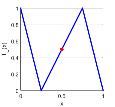
A specific random driving could be given by for some and for and , but only the ergodicity of will be important for us. Setting it is immediate that (E1), (E2), (E3), and ((E4)) hold.
We select a measurable family of observation functions . For a.e. , is , has a unique maximum at , and is a locally even function about . For small we will then have that is a small neighbourhood of , satisfying ((E5)) and ((A)). In light of Remark 2.5.3 and Proposition 2.5.5 we see that ((X)) holds. The corresponding cocycle of open operators satisfy ((MC)). Given an essentially bounded function , the are chosen to satisfy ((S)). Because the are with unique maxima and is Lebesgue for all we can make such a choice of with55 5 In the situation where is constant a.e. for each , in general we cannot satisfy ((S)) for a given fixed scaling function . In the case where is also constant a.e. if is random but sufficiently close to a non-random observation for each , we can satisfy ((S)) by incorporating the error term . This situation corresponds to a decreasing family of holes whose length fluctuates slightly in with the fluctuation decreasing to zero sufficiently fast. A similar situation can occur if the scaling function is a general measurable function. These situations motivate the use of the error term in condition ((S)). . Furthermore, as is Lebesgue we have that ((S)) implies that assumption (E6) is automatically satisfied. With the above choices, (E7) is clearly satisfied for . To show condition (E8) with we note that , while . Therefore we require , which by elementary rearrangement is always true for . Because there is a full branch outside the branch with the hole, ((E9)) is satisfied with and .
At this point we have checked all of the hypotheses of Theorem 2.5.12 and we obtain that for sufficiently small holes as defined above, the corresponding random open dynamical system has a quenched thermodynamic formalism and quenched decay of correlations. We note that this result does not require ((S)); the holes do not need to scale in any particular way with , they simply need to be sufficiently small. In order to next apply Theorem 2.4.5 we do require ((S)) and additionally ((C8)).
To finish the example, we verify ((C8)). We claim that for each fixed , one has for sufficiently sufficiently large (sufficiently small ). If this were not the case, there must be a positive -measure set of points that (i) lie in , (ii) land outside the sequence of holes for the next iterations, and then (iii) land in on the iteration. In this example, because all are neighbourhoods of of diameter smaller than , and the maps are locally expanding about , for fixed one can find a large enough so that it is impossible to leave a small neighbourhood of and return after iterations. For , by definition
| (2.7.2) |
There are two cases to consider:
Case 1: is larger than the local preimage of ; that is, . Because of the linearity of the branch containing , one has .
Case 2: is smaller than the local preimage of ; that is, . By (2.7.2) and ((S)) we then have
and thus for such an , . Thus, combining the two cases,
exists for a.e. , verifying ((C8)).
Recalling that , we may now apply Theorem 2.4.5 to obtain the quenched extreme value law:
| (2.7.3) | |||||
This formula is a generalization of the formula in Remark 8 [55], where we may create nontrivial laws from either the random dynamics , or the random scalings , or both. The following two special cases consider these mechanisms separately.
- (1)
Random maps, non-random scaling ( takes a constant value ): Since , in this case (2.7.3) becomes
(2.7.4) and we see that we can interpret as an extremal index.
- (2)
Fixed map, random scaling: Suppose ; then we may replace with in (2.7.3), and we see we the extremal index depends on the choice of random scalings alone; of course the thresholds depend on the chosen .
Similar results could be obtained with the possessing nonlinear branches. The arguments above can also be extended to the case where is a periodic point of prime period for all maps; the formula (2.7.3) now includes and . If the scaling is non-random, one would simply replace in (2.7.4) with .
We recall that for deterministic (including non-uniformly hyperbolic maps), the extremal index enjoys a dichotomy, in the sense that it is equal to when a single hole shrinks to an aperiodic point, and it is strictly smaller than when the hole shrinks to a periodic point. In the latter case the extremal index can be expressed in terms of the period; see [62] for a general account of the above facts. Example 2.7.1 shows that in a simple random setting there are many more ways to obtain nontrivial exponential limit laws, e.g. by random scaling, or by the existence of periodic orbits for only a positive measure set of .
Example 2.7.2.
Random -maps, random holes containing a non-random fixed point (random observations with non-random maximum), general geometric potential
We show how a nontrivial extremal index can arise from random -maps where statistics are generated by an equilibrium state of a general geometric potential. Consider the “no short branches” random -map example of Section 13.2 [3], where for a.e. , and some and . The measurability of yields ((M1)). We use the weight , . To obtain ((MC)) the base dynamics is driven by an ergodic homeomorphism on a Borel subset of a separable, complete metric space, assuming that has countable range, as in Example 2.7.1. Our random observation function is measurable and for a.e. , is with a unique maximum at . We select a measurable scaling function ; either or both of and could be -independent. By assigning thresholds (which could also be -independent) we obtain a decreasing family of holes , which are decreasing intervals with left endpoint at .
Clearly (E2) and (E3) hold and Lemma 13.5 [3] provides ((E4)). Conditions ((E5)) and (E6), and ((A)) are immediate, as is (E7) with . Condition ((EX)) holds because there is at least one full branch outside the branch with the hole. Regarding (E8), and arguing as in the previous example, since , we see (E8) holds with because . Because there is at least one full branch outside the branch with the hole, ((E9)) holds with and . We have now checked all of the hypotheses of Theorem 2.5.12. By this theorem, for sufficiently small holes , the corresponding random open dynamical system has a quenched thermodynamic formalism and quenched decay of correlations. As in the previous example, we emphasise that this result does not require ((S)).
Because is uniformly bounded above and below, as long as is random, we may adjust to obtain ((S)). We now verify ((C8)) for our holes, which are of the form , in preparation to apply Theorem 2.4.5. The same arguments from Case 1 and Case 2 of the previous example apply. Case 2 is unchanged. In Case 1 we have
Because is a finite union of left-closed intervals, using the fact that , and therefore has left- and right-hand limits everywhere, we may redefine at the finite collection of points so that
recalling that in Case 1, . Taking the minimum of Cases 1 and 2 as in Example 2.7.1, we see that exists, which verifies ((C8)). Finally,
| (2.7.5) |
Example 2.7.3.
A fixed map with random holes containing a fixed point (random observations with a non-random maximum)
Let us now consider more closely the case of a fixed map and holes moving randomly around a fixed point , a situation previously considered in [11] in the annealed framework.
We take a piecewise uniformly expanding map of the unit interval of class , and such that is surjective on the domains of local injectivity. Moreover preserves a mixing measure equivalent to the Lebesgue measure with strictly positive density . We moreover assume that and are continuous at a fixed point . The observation functions have a common maximum at , leading to holes that are closed intervals containing the point for any . In Example 2.7.1 the holes were centered on but could vary dramatically in diameter between -fibers. In this example the holes need not be centered on but must become more identical as they shrink. Specifically, we assume
| (2.7.6) |
where the use of Lebesgue is for simplicity.
Since the sample measures coincide with we may easily verify condition ((S)) by choosing conveniently the size of the hole . Moreover, by choosing the holes to be contained entirely within exactly one interval of monotonicity, we see that ((EX)) holds, and thus ((X)) holds via Remark 2.5.3 and Proposition 2.5.5. Since the weights are nonrandom and equal to conditions (E1) to (E7) clearly hold. Since is continuous in , the holes will belong to one branch of Therefore if will denote the number of branches of and it will be enough to have in order to satisfy ((E9)) with Moreover, still keeping and since we have finitely many branches, condition ((E9a)) in Remark 2.C.2 is satisfied with . We may now apply Theorem 2.5.12 to obtain a quenched thermodynamic formalism for our fixed map with sufficiently small random holes.
Whenever the point is not periodic, one obtains that all the are zero by repeating the argument given in Example 2.7.1 for and using the continuity of at . We now take as a periodic point of minimal period and we assume that and are continuous at . We now begin to evaluate
| (2.7.7) |
Since is continuous and expanding in the neighborhood of , by taking large enough, the set has only one connected component. Denote the local branch of through by . Therefore by a local change of variable we have for the upper bound of the numerator
| (2.7.8) | |||||
For the lower bound of the numerator, since is locally expanding, , and by (2.7.8)
We can bound the second negative term as
We are now in a position to verify the existence of the limit . Using the above bounds we have
Example 2.7.4.
Random maps with random holes
We saw in Examples 2.7.1 and 2.7.3 that an extremal index less than one could be obtained for observables reaching their maximum around a point which was periodic for all the random maps, or, for a fixed map, when the holes shrink around the periodic point. We now produce an example where periodicity is not responsible for getting an extremal index less than one. This example is the quenched version of the annealed cases investigated in sections 4.1.2 and 4.2.1 of the paper [21].
Let with the bilateral shift map, and an invariant ergodic measure. To each letter we associate a point in the unit circle and we consider the well-known observable in the extreme value theory literature:
where denotes the -th coordinate of
In this case the hole will be the ball of center and radius . For each we associate a map where are maps of the circle which we will take as -maps of the form66 6 The reason for this choice is that, in order to compute the quantities , we have to follow the itinerary of the points under the composition of the maps and compare with their predecessors. As it will be clear in the computation below for and the task will be relatively easy and generalizable to any , if all the maps are at least which in particular means that the image of the point is not a discontinuous point of the . It will also be true that all the maps are differentiable with bounded derivative in small neighbourhoods of any . If these conditions are relaxed, it could be that the limit defining the for some is not immediately computable, we defer to section 3.3 and Proposition 3.4 in [8] for a detailed discussion of the computation of the extremal index in presence of discontinuities. Another advantage of our choice is that, as in Example 2.7.1, all the sample measure are equivalent to Lebesgue, , with , , and . Since the range of is finite and the shift is a homeomorphism on with respect to the usual metrics for , assumption ((MC)) is verified. Since the potential is equal to conditions (E1) to (E7) clearly hold. Condition (E8) holds as in Example 2.7.1, which uses similar piecewise linear expanding maps. Condition ((E9)) is a consequence of the fact that we have finitely many maps each of which is full branches; it will be therefore enough to invoke ((E9a)) with As we have chosen we have that ((EX)) holds and thus ((X)) follows via Proposition 2.5.5.
At this point we may apply Theorem 2.5.12 to obtain a quenched thermodynamic formalism for sufficiently small holes.
As a more concrete example, we will consider an alphabet of four letters and we set the associations
where the points , are chosen on the unit interval according to the following prescriptions:
| (2.7.9) |
Since the sample measures coincide with the Lebesgue measure, condition ((S)) reduces to and we can solve for by setting . The prescription (2.7.9) clearly avoids any sort of periodicity when we take the first iteration of the random maps needed to compute nevertheless we will show that and this is sufficient to conclude that is smaller than . Of course we need to prove that the limits defining all the other for any exist. We will show it for and the same arguments could be generalized to any
Using -invariance of Lebesgue, we have (for simplicity we write instead of ):
provided the limit exists, which we are going to establish. Consider first a point in the cylinder ; the quantity we have to compute is therefore
| (2.7.10) |
If is large enough, by the prescription (2.7.9), we see that the local preimage of under will be strictly included into and its length will be contracted by a factor Therefore the ratio (2.7.10) will be simply The same happens with the cylinders and producing respectively the quantities and For all the other cylinders the ratio will be zero since the sets entering the numerator of (2.7.10) will be disjoint for large enough. In conclusion we have
If we now take , -independent, and we choose as the Bernoulli measure with equal weights , the preceding expression assumes the simpler form
To compute we have to split the integral over cylinders of length three. As a concrete example let us consider the cylinder where By using the preceding notations, we have to control the set
Let us first consider the intersection Call one of the preimages of and the inverse branch giving . If then the intersection is empty. Otherwise, by taking large enough, the set will be completely included in and moreover we have, by the linearity of the maps, We are therefore left with the computation of If we proceed as in the computation of by using the prescriptions (2.7.9); otherwise such an intersection will be empty for large enough. For instance, if, in the example we are considering, we take and we suppose that among the preimages of there is, besides too, namely and no other element of 77 7 This condition does not intervene to compute and shows that it is strictly less than one. then we get the contribution for
From the above it follows that exists for a.e. , and that we may apply Theorem 2.4.5.
It is not difficult to give an example where all the can be explicitly computed. Let us take our beta maps - in the particular case where all the are equal to the irrational number Then take a sequence of random balls with the centers which are rational numbers. From what we discussed above, it follows that a necessary condition to get a is that the center will be sent to the center Let one of this rational centers; the iterate has the form -mod where is an integer number. Therefore such an iterate will be never a rational number which shows that all the for any and and therefore
Chapter 2 Appendices
Appendix 2.A A version of [39] with general weights
In this appendix we outline how to extend relevant results from [39] from the Perron–Frobenius weight to the general class of weights in Section 2.5. To begin, we note that there is a unique measurable equivariant family of functions guaranteed by Theorem 2.19 [3] (called there). We wish to obtain uniform control on the essential infimum and essential supremum of for a suitable class of maps.
In [39] we work with the space and use the norm . Here we have a measurable family of random conformal probability measures (guaranteed by Theorem 2.19 [3]) and we work with the random spaces and the random norms . We also work with the normalised transfer operator . All of the variation axioms (V1)–(V8) in [39] hold with the obvious replacements.
Proof of Lemma 2.5.9.
C7’ (): We show ; this will give us ((C7’)). The statement is a generalized version of Lemmas 1 and 5 [39] and we follow the strategy in [39]. The result follows from Lemma 2.A.2 below, which in turn depends on (2.A.3) and Lemma 2.A.1.
C4’ (): It will be sufficient to show that there is a and such that for all with and a.e. , one has
| (2.A.1) |
This is a generalized version of Lemma 2 [39], which has an identical proof, making the replacements outlined in the proof of Lemma 2.A.1 below, and using Lemmas 2.A.1–2.A.5 and (2.A.3). We also use the non-random equivalence (2.5.13) of the norm to the usual norm.
C2 (), C3 (), C5’ (): We wish to show that there is a unique measurable, nonnegative family with the property that , , for a.e. , , and
| (2.A.2) |
We note that again the norm equivalence (2.5.13). This is a generalized version of Proposition 1 [39]. To obtain this generalization, in the proof of Proposition 1 [39], one modifies the space to become
All of the arguments go through as per [39] with the appropriate substitutions. Our modified proof of Proposition 1 [39] will also use the modified Lemmas 2.A.1–2.A.5, and inequality (2.A.3) below.
CCM: Finally, we note that ((CCM)) follows from ((C2)) () together with non-atomicity of . But non-atomicity of follows from the random covering assumption as in the proof of Proposition 3.1 [3]
Full Support: Following the proof of Claim 3.1.1 of [3], we are able to show that is fully supported on , i.e. for any non-degenerate interval . ∎
We note that by (2.5.19) with , we have our uniform Lasota–Yorke equality.
| (2.A.3) |
for all and a.e. . This immediately provides a suitable general version of ((H2)) [39], which is that there is a such that
| (2.A.4) |
Define random cones .
Lemma 2.A.1 (General weight version of Lemma A.1 [39]).
For sufficiently large we have that for sufficiently large and a.e. .
Proof.
Identical to [39], substituting for , for , and for Lebesgue. ∎
Lemma 2.A.2 (General weight version of Lemma 1 [39]).
If one has uniform covering in the sense of (11) [39], then there is an such that for each and sufficiently large , there exists such that
| (2.A.5) |
Proof.
Making all of the obvious substitutions, as per Lemma 2.A.1 and its proof, we subdivide the unit interval into an equipartition according to mass. This is possible because is non-atomic (Proposition 3.1 [3]). We conclude, as in the proof of Lemma 1 [39], that there is an interval of -measure such that for each one has . Then using uniform covering and the facts that , , and , we obtain , where is the uniform covering time for the interval . The rest of the proof follows as in [39]. ∎
Lemma 2.A.3 (General weight version of Lemma A.2 [39]).
Assume that and . Then .
Proof.
Identical to [39], substituting for Lebesgue. The randomness of the Hilbert metric only appears because the functions lie in . ∎
Lemma 2.A.4 (General weight version of Lemma A.3 [39]).
For any , we have that is a contraction on for any sufficiently large and a.e. .
Proof.
Let .
Lemma 2.A.5 (General weight version of Lemma A.4 [39]).
Proof.
Lemma 2.A.6 (General weight version of Lemma 5 [39]).
for a.e. .
Proof.
Identical to [39] with the appropriate substitutions. ∎
Appendix 2.B A summary of checks that relevant results from [27] can be applied to
The stability result Theorem 4.4 [27] assumes that the underlying Banach space is separable, however this separability assumption is only used to obtain measurability of various objects (and in fact Theorem 3.4 [27] may be applied to sequential dynamics). We use these results for the non-separable space in the proof of Lemma 2.5.10, and we therefore need to check that all relevant results in [27] hold for , under the -continuity assumption on ; the latter will provide the required measurability. All section, theorem, proposition, and lemma numbers below refer to numbering in [27].
There are no issues of measurability in Section 3, including Theorem 3.4, until Section 4, so we begin our justifications from Section 4.
We now fix some notation from [27] which will be used only in this section. For each , let be a Banach space and a normal Saks space88 8 A Saks space is a Banach space equipped with a second locally convex topology that is coarser than the norm topology such that the closed unit ball in the norm topology is closed and bounded in the -topology. In our setting we take the -topology to be the one generated by the second norm .. For a thorough treatment of Saks spaces see the seminal work of Cooper [25], and for an introduction into Saks spaces for dynamical systems see [27]. Let , and let denote the projection onto . Let denote the collection of bounded linear operators from to and let denote the set of bounded linear endomorphisms of covering , i.e.
where is given by . We now introduce the notion of a hyperbolic splitting from [27]. We denote the norm on by , the norm on by , and the norm on by .
Definition 2.B.1 (Definition 3.1 of [27]).
Suppose that , , , and . We say that and form a -hyperbolic splitting for , and that has a hyperbolic splitting index , if there exists constants such that:
- (H1)
For every we have and
- (H2)
For each we have . Moreover, for every and we have
- (H3)
For each we have and for every we have
We call and the equivariant fast and slow spaces for , respectively.
Let denote the collection of operators which satisfy the following uniform Lasota-Yorke inequality: for each , , and we have
We let denote the set of all Saks space equicontinuous endomorphisms meaning that and for each there exists such that for every and
Finally, if , then for each set
For the convenience of the reader, we restate Theorem 4.4 of [27] here.
Theorem 2.B.2.
Suppose that is a Saks space, with a Banach space, that is a separable strongly measurable random linear system with ergodic invertible base and a uniform hyperbolic Oseledets splitting of dimension , and that for some and . There exists such that if is a separable strongly measurable random linear system with , then also has an Oseledets splitting of dimension . In addition, letting () be the Lyapunov exponents of , there exists such that each () separates the Lyapunov spectrum of , and the corresponding projections satisfy
and
Moreover, for every there exists so that if , then
and
We now describe the necessary changes in order to apply Theorem 4.4 to our setting. Theorem, Proposition, Lemma, and equation numbers below refer to numbers in [27].
Theorem 4.4 (Theorem 2.B.2): This is the main stability theorem. We would substitute “separable strongly measurable random dynamical system” with “-continuous random dynamical system”. This theorem relies on Propositions 4.6 and 4.7, Lemma 4.11, Proposition 4.12, and Lemma 4.13.
Proposition 4.6: There is no measurability involved.
Proposition 4.7: Uses Lemmas 4.8 and 4.10. We note that the bounds (93)–(95) in the proof are simpler in our application of this result as our top space is one-dimensional.
Lemma 4.8: This may be replaced by Theorem 17 [45], which treats the -continuous setting. This removes any use of Proposition B.1 and Lemma B.7.
Lemma 4.9: This uses Lemma 4.8 and the fact that compositions of -continuous maps are -continuous. The latter replaces the use of Lemma A.5 [48], which is used in several results. This replacement will not be mentioned further.
Lemma 4.10: We will assume that is -continuous in the statement of the lemma. At the start of the proof we would now instead have is -continuous by the definition of -continuity (see e.g. (4) in [45]); this removes the use of Lemma B.2 in the proof. Lian’s thesis is quoted regarding measurable maps/bases connected with a measurable space . In our application, has rank 1 and therefore stating that there is a (in our case -continuous) map is trivial. One proceeds similarly for the dual basis.
Lemma 4.11: This concerns measurability and integrability of and where is an Oseledets space. -continuity of is provided by Theorem 17 [45], removing the need for Lemma B.2. The -continuity of follows from Lemma 7 [45]. Because in our application setting we only require one-dimensional , the determinants are given by norms and there is nothing more to do concerning determinants. This removes the need for Proposition B.8. Lemma B.16 [48] may be replaced with Lemma 7 [45] to cover the -continuous setting. Proposition B.6 is not required in the -continuity setting.
Proposition 4.12: There is no measurability involved.
Lemma 4.13: There is no measurability involved.
Appendix 2.C A var– Lasota–Yorke inequality
Recall from Section 2.5 that denotes the partition of monotonicity of and that is the collection of all finite partitions of such that
| (2.C.1) |
for each . Given , we set where is the coarsest partition amongst all those finer than and such that all elements of are either disjoint from or contained in . Then (2.C.1) implies that
| (2.C.2) |
for each . We now prove a Lasota–Yorke inequality inspired by Lemma 1.5.1.
Lemma 2.C.1.
For any we have
Proof.
Since , if , then , and thus, we have for each . Thus, considering only the intervals in , we are able to write
| (2.C.3) |
where
is the inverse branch which takes to for each . Now, since
we can rewrite (2.C.3) as
| (2.C.4) |
So,
| (2.C.5) |
Now for each , using the fact that and (2.C.2) we have
| (2.C.6) |
Using (2.C.6), we may further estimate (2.C.5) as
| (2.C.7) | |||||
and thus we are done. ∎
Remark 2.C.2.
Note that we could have used Leb or any probability measure in (2.C.6) rather than . Furthermore, Lemma 2.C.1 could be applied to Section 2.5 with a measure other than if the appropriate changes are made to the assumption ((E9)) so that a uniform-in- lower bound similar to (2.5.18) may be calculated.
In particular if we replace ((E9)) with the following:
- (E9a)
There exists and such that for -a.e. , all sufficiently small, we have for all ,
- (E9b)
There exists such that ,
then the claims of Section 2.5 hold with in (2.C.6) replaced with Leb.
Indeed, to obtain a replacement for (2.5.18) one could use ((E9a)) and ((E9b)) to get
for all , where we have also used (E3) for the final inequality. As ((E9)) is only used to prove (2.5.18), the remainder of Section 2.5 can be carried out with the appropriate notational changes. In fact, the proof of Lemma 2.5.10 can be simplified by replacing with Leb as Lemma 5.2 of [14] would no longer be needed.
Appendix 2.D Proof of Claim (6) of Theorem 2.5.12
Proof of Claim (6) of Theorem 2.5.12:
Set . Define the fully normalized operator given by
Then we have that and . Following the proof of Theorem 1.11.2, we can prove the following similar statement to Claim (5) of Theorem 2.5.12: For each , -a.e. and all we have
| (2.D.1) |
where and , are as in Claim (5) of Theorem 2.5.12. Using standard arguments (see Theorem 11.1 [3]) we have that
Note that at this stage we are unable to apply (2.D.1) as the norm and the measure are incompatible. Now from the third statement of Claim (5) of Theorem 2.5.12 we have that
and thus we must have that
| (2.D.2) |
Using (2.D.1) and (2.5.14), we have that
| (2.D.3) |
Combining (2.D.2) and (2.D.3) and using (2.D.1) again we see that
for all sufficiently large, and thus the proof of Claim (6) of Theorem 2.5.12 is complete.
∎
Chapter 3 Open Questions and Future Directions
In this final chapter we present several open questions and directions that have yet to be explored.
3.1. Questions from Chapter 1
Question 3.1.1.
Can the hypotheses ((Q1)) on the maximum number of contiguous “bad” intervals be weakened or removed for “large” holes?
Chapter 2 answered this question in the affirmative for “small” holes, meaning holes that are taken to be sufficiently small such that a perturbation theory applies. However, it is not clear at all whether this assumption can be removed or weakened in the case of “large” holes. Furthermore, the assumptions on the contiguous “bad” intervals does not translate well to higher dimensional systems, so it seems necessary to develop a better assumption in order to develop the theory of “large hole” open dynamical systems for higher dimensions.
Question 3.1.2.
Can the hypotheses of large images and large images with respect to be removed from Theorem 1.14.4?
This question is answered in the affirmative for a large class of expanding random interval maps with holes in an upcoming work of the first author and Nathan Dalaklis.
Question 3.1.3.
Are finer statistical limit laws applicable to open dynamical systems?
In [22] (see also [23, Theorem 8.34]) the authors prove a “conditioned” Central Limit Theorem for ACCIMs (referred to there as quasi-stationary distributions) in the context of finite state Markov chains, where the relevant measure is conditioned on the surviving sets . Within the language Chapter 1, Collet and Martínez prove that for sufficiently “nice” observables and ACCIMs
It begs the question whether a similar result holds for our random open systems and whether stronger statistical limit laws can be proven in either the deterministic or random settings.
Question 3.1.4.
Can our approach to thermodynamic formalism for random open systems be extended to random higher dimensional piecewise expanding or hyperbolic systems?
The approach of Chapter 1 heavily relies on the geometry of the interval. In particular, there appears to be no straightforward generalization of our assumption ((Q1)) to higher dimensions. If one is willing to consider small holes, the perturbative approach of Chapter 2, in particular Section 2.5, offers a promising approach. Even still, one must then find a suitable Banach space in which to work, as BV is not necessarily the most useful space for higher dimensions. The quasi-Hölder, or Keller spaces [54], could be a suitable option as it has been used in both higher dimensions [69] as well as open systems [40, 67].
3.2. Questions from Chapter 2
Question 3.2.1.
Can the perturbative approach to thermodynamic formalism for random open systems taken in Section 2.5 be used on other (closed) random dynamical systems?
The perturbative approach to open dynamical systems has been investigated previously in the deterministic setting in [60, 40, 43, 67, 18]. Can the perturbative approach be used to prove thermodynamic formalism results, like Theorem A, in other random settings, e.g. [65]?
Question 3.2.2.
In [5], we have adapted this approach to prove that the sequence of random variables that count the number of returns to a sequence of random shrinking targets converges to a compound Poisson distribution. In particular, it is shown that under the assumption of the scaling ((S)), the distributions
converge almost surely to a compound Poisson random variable. One can then ask what further results can be obtained with this spectral approach. Can the techniques Chapter 2 and [5] be adapted to prove stable laws?
Question 3.2.3.
Can asymptotic formulas for the change in the Hausdorff dimension of the perturbed random surviving sets be found in the style of Theorem 2.3.7?
In [67] Pollicott and Urbański find asymptotic results [67, Theorem 1.0.9], with a similar flavor to Theorem 2.3.7, for the Hausdorff dimension of the (deterministic) perturbed surviving set as in the setting of conformal graph directed Markov systems. Can such a result be proven in the random setting for the interval maps of Section 2.5 in either the presence or absence of the large images property? In particular, what can be said of the existence and/or value of the limiting quantity
Acknowledgments
The authors thank Harry Crimmins and Yushi Nakano for helpful discussions. JA, GF, and CG-T thank the Centro de Giorgi in Pisa and CIRM in Luminy for their support and hospitality. JA is supported by the ARC Discovery projects DP180101223 and DP210100357, and thanks the School of Mathematics and Physics at the University of Queensland for their hospitality. GF, CG-T, and SV are partially supported by the ARC Discovery Project DP180101223. The research of SV was supported by the project Dynamics and Information Research Institute within the agreement between UniCredit Bank R&D group for financial support through the “Dynamics and Information Theory Institute” at the Scuola Normale Superiore di Pisa and by the Laboratoire International Associé LIA LYSM, of the French CNRS and INdAM (Italy). The authors thank an anonymous referee for their helpful comments and bibliographic suggestions.
Bibliography
- [1] Ludwig Arnold. Random Dynamical Systems. Springer Monographs in Mathematics. Springer Berlin Heidelberg, Berlin, Heidelberg, 1998.
- [2] Jason Atnip. An Almost Sure Invariance Principle for Several Classes of Random Dynamical Systems. 2017. Preprint: arXiv: 1702.07691.
- [3] Jason Atnip, Gary Froyland, Cecilia González-Tokman, and Sandro Vaienti. Thermodynamic Formalism for Random Weighted Covering Systems. Communications in Mathematical Physics, July 2021.
- [4] Jason Atnip, Gary Froyland, Cecilia González-Tokman, and Sandro Vaienti. Equilibrium states for non-transitive random open and closed dynamical systems. Ergodic Theory and Dynamical Systems, pages 1–23, October 2022.
- [5] Jason Atnip, Gary Froyland, Cecilia González-Tokman, and Sandro Vaienti. Compound Poisson statistics for dynamical systems via spectral perturbation. Preprint: arXiv:2308.10798, February 2024.
- [6] Jason Atnip, Hiroki Sumi, and Mariusz Urbański. The Dynamics and Geometry of Semi-Hyperbolic Rational Semigroups. To appear in Memoirs of the AMS. arXiv:2004.13990, 2020.
- [7] Jason Atnip and Mariusz Urbański. Critically finite random maps of an interval. Discrete & Continuous Dynamical Systems - A, 40(8):4839, 2020.
- [8] H. Aytac, J.M. Freitas, and S. Vaienti. Laws of rare events for deterministic and random dynamical systems. Trans. Amer Math. Soc., 367:8229–8278, 2015.
- [9] Kazuopki Azuma. Weighted sums of certain dependent random variables. Tôhoku Math. Journ., 19(3):357–367, 1967.
- [10] Wael Bahsoun, Jörg Schmeling, and Sandro Vaienti. On transfer operators and maps with random holes. Nonlinearity, 28(3):713–727, March 2015.
- [11] Wael Bahsoun and Sandro Vaienti. Escape rates formulae and metastablilty for randomly perturbed maps. Nonlinearity, 26(5):1415–1438, May 2013.
- [12] Garrett Birkhoff. Lattice Theory. American Mathematical Society, New York, 1940.
- [13] Thomas Bogenschütz and Volker Matthias Gundlach. Ruelle’s Transfer Operator for Random Subshifts of Finite Type. Ergod. Th. & Dynam. Sys, 15:413–447, 1995.
- [14] Christopher Bose, Gary Froyland, Cecilia González-Tokman, and Rua Murray. Ulam’s method for Lasota–Yorke maps with holes. SIAM Journal on Applied Dynamical Systems, 13(2):1010–1032, 2014.
- [15] Rufus Bowen. Hausdorff dimension of quasi-circles. Publications Mathématiques de l’IHÉS, 50:11–25, 1979.
- [16] A. Boyarsky and P. Gòra. Laws of Chaos. Birkhäuser, 1997.
- [17] Rainer Brück and Matthias Büger. Generalized iteration. Computational Methods and Function Theory, 3(1-2, [On table of contents: 2004]):201–252, 2003.
- [18] Henk Bruin, Mark F. Demers, and Mike Todd. Hitting and escaping statistics: mixing, targets and holes. Advances in Mathematics, 328:1263–1298, April 2018.
- [19] Henk Bruin and Mike Todd. Equilibrium States for Interval Maps: Potentials with . Communications in Mathematical Physics, 283(3):579–611, November 2008.
- [20] Jérôme Buzzi. Exponential Decay of Correlations for Random Lasota-Yorke Maps. Communications in Mathematical Physics, 208(1):25–54, 1999.
- [21] Théophile Caby, Davide Faranda, Sandro Vaienti, and Pascal Yiou. On the computation of the extremal index for time series. Journal of Statistical Physics, 179:1666–1697, 2020.
- [22] P. Collet and S. Martínez. Diffusion coefficient in transient chaos. Nonlinearity, 12(3):445, May 1999.
- [23] Pierre Collet, Servet Martínez, and Jaime San Martín. Quasi-stationary distributions. Probability and its Applications (New York). Springer, Heidelberg, 2013. Markov chains, diffusions and dynamical systems.
- [24] Pierre Collet, Servet Martínez, and Véronique Maume-Deschamps. On the existence of conditionally invariant probability measures in dynamical systems. Nonlinearity, 13(4):1263–1274, June 2000.
- [25] J. B. Cooper. Saks spaces and applications to functional analysis, volume 139 of North-Holland Mathematics Studies. North-Holland Publishing Co., Amsterdam, second edition, 1987.
- [26] Hans Crauel. Random probability measures on Polish spaces, volume 11 of Stochastics Monographs. Taylor & Francis, London, 2002.
- [27] Harry Crimmins. Stability of hyperbolic Oseledets splittings for quasi-compact operator cocycles. DCDS, 42(6):2795–2857, June 2022. Publisher: Discrete and Continuous Dynamical Systems.
- [28] Mark Demers, Paul Wright, and Lai-Sang Young. Escape Rates and Physically Relevant Measures for Billiards with Small Holes. Communications in Mathematical Physics, 294(2):353–388, March 2010.
- [29] Mark F. Demers. Escape rates and physical measures for the infinite horizon Lorentz gas with holes. Dynamical Systems, 28(3):393–422, September 2013.
- [30] Mark F. Demers and Bastien Fernandez. Escape rates and singular limiting distributions for intermittent maps with holes. Transactions of the American Mathematical Society, 368(7):4907–4932, December 2015.
- [31] Mark F. Demers and Mike Todd. Equilibrium states, pressure and escape for multimodal maps with holes. Israel Journal of Mathematics, 221(1):367–424, September 2017.
- [32] Mark F. Demers and Mike Todd. Slow and Fast Escape for Open Intermittent Maps. Communications in Mathematical Physics, 351(2):775–835, April 2017.
- [33] Mark F. Demers and Mike Todd. Asymptotic escape rates and limiting distributions for multimodal maps. Ergodic Theory and Dynamical Systems, pages 1–50, March 2020.
- [34] Mark F. Demers, Paul Wright, and Lai-Sang Young. Entropy, Lyapunov exponents and escape rates in open systems. Ergodic Theory and Dynamical Systems, 32(4):1270–1301, August 2012.
- [35] Manfred Denker, Gerhard Keller, and Mariusz Urbański. On the uniqueness of equilibrium states for piecewise monotone mappings. Studia Mathematica, 97(1):27–36, 1990.
- [36] Manfred Denker and Mariusz Urbański. On the existence of conformal measures. Transactions of the American Mathematical Society, 328(2):563–587, 1991.
- [37] Davor Dragičević and Yeor Hafouta. Almost sure invariance principle for random distance expanding maps with a nonuniform decay of correlations. In Thermodynamic formalism, volume 2290 of Lecture Notes in Math., pages 177–204. Springer, Cham, [2021] ©2021.
- [38] D. Dragičević, G. Froyland, C. González-Tokman, and S. Vaienti. A Spectral Approach for Quenched Limit Theorems for Random Expanding Dynamical Systems. Communications in Mathematical Physics, 360(3):1121–1187, June 2018.
- [39] Davor Dragičević, Gary Froyland, Cecilia González-Tokman, and Sandro Vaienti. Almost sure invariance principle for random piecewise expanding maps. Nonlinearity, 31(5):2252–2280, May 2018.
- [40] Andrew Ferguson and Mark Pollicott. Escape rates for Gibbs measures. Ergodic Theory and Dynamical Systems, 32(03):961–988, June 2012.
- [41] A.C.M. Freitas, J.M. Freitas, and M. Todd. Hitting time statistics and extreme value theory. Probab. Theory Related Fields, 147(3):675–710, 2010.
- [42] Ana Cristina Moreira Freitas, Jorge Milhazes Freitas, Mario Magalhaes, and Sandro Vaienti. Point processes of non stationary sequences generated by sequential and random dynamical systems. Journal of Statistical Physics, 181:1365–1409, 2020.
- [43] Ana Cristina Moreira Freitas, Jorge Milhazes Freitas, and Mike Todd. Speed of convergence for laws of rare events and escape rates. Stochastic Process. Appl., 125(4):1653–1687, 2015.
- [44] Ana Cristina Moreira Freitas, Jorge Milhazes Freitas, and Sandro Vaienti. Extreme value laws for non stationary processes generated by sequential and random dynamical systems. Annales de l’Institut Henri Poincaré, 53(3):1341–1370, 2017.
- [45] Gary Froyland, Simon Lloyd, and Anthony Quas. A semi-invertible Oseledets Theorem with applications to transfer operator cocycles. Discrete and Continuous Dynamical Systems, 33(9):3835–3860, March 2013.
- [46] Gary Froyland and Ognjen Stancevic. Metastability, lyapunov exponents, escape rates, and topological entropy in random dynamical systems. Stochastics and Dynamics, 13(04):1350004, December 2013. Publisher: World Scientific Publishing Co.
- [47] Brett Geiger and William Ott. Nonstationary open dynamical systems. arXiv:1808.05315 [math], May 2020. arXiv: 1808.05315.
- [48] Cecilia González-Tokman and Anthony Quas. A semi-invertible operator Oseledets theorem. Ergodic Theory and Dynamical Systems, 34(4):1230–1272, 2014.
- [49] Franz Hofbauer and Gerhard Keller. Equilibrium states for piecewise monotonic transformations. Ergodic Theory and Dynamical Systems, 2(1):23–43, March 1982.
- [50] Franz Hofbauer and Gerhard Keller. Ergodic properties of invariant measures for piecewise monotonic transformations. Math. Z., 180:119–140, 1982.
- [51] J. Hüsler. Asymptotic approximation of crossing probabilities of random sequences. Z. Wahrsch. Verw. Gebiete, 63(2):257–270, 1983.
- [52] J. Hüsler. Extreme values of nonstationary random sequences. J. Appl. Probab., 23(4):937–950, 1986.
- [53] Irene Inoquio-Renteria and Juan Rivera-Letelier. A characterization of hyperbolic potentials of rational maps. Bull. Braz. Math. Soc. (N.S.), 43(1):99–127, 2012.
- [54] Gerhard Keller. Generalized bounded variation and applications to piecewise monotonic transformations. Zeitschrift für Wahrscheinlichkeitstheorie und Verwandte Gebiete, 69(3):461–478, 1985.
- [55] Gerhard Keller. Rare events, exponential hitting times and extremal indices via spectral perturbation†. Dynamical Systems, 27(1):11–27, 2012.
- [56] Gerhard Keller and Carlangelo Liverani. Stability of the spectrum for transfer operators. Annali della Scuola Normale Superiore di Pisa - Classe di Scienze, 28(1):141–152, 1999. Publisher: Scuola normale superiore.
- [57] Gerhard Keller and Carlangelo Liverani. Rare Events, Escape Rates and Quasistationarity: Some Exact Formulae. Journal of Statistical Physics, 135(3):519–534, 2009.
- [58] M.R. Leadbetter, G. Lindgren, and H. Rootzen. Extremes and related properties of random sequences and series. 1983.
- [59] Carlangelo Liverani. Decay of correlations for piecewise expanding maps. Journal of Statistical Physics, 78(3):1111–1129, February 1995.
- [60] Carlangelo Liverani and Véronique Maume-Deschamps. Lasota–Yorke maps with holes: conditionally invariant probability measures and invariant probability measures on the survivor set. Annales de l’Institut Henri Poincare (B) Probability and Statistics, 39(3):385–412, May 2003.
- [61] Carlangelo Liverani, Benoit Saussol, and Sandro Vaienti. Conformal measure and decay of correlation for covering weighted systems. Ergodic Theory and Dynamical Systems, 18(6):1399–1420, December 1998.
- [62] Valerio Lucarini, Davide Faranda, Ana Cristina Moreira Freitas, Jorge Milhazes Freitas, Mark Holland, Tobias Kuna, Matthew Nicol, Mike Todd, and Sandro Vaienti. Extremes and recurrence in dynamical systems. 2016.
- [63] Philip T. Maker. The ergodic theorem for a sequence of functions. Duke Mathematical Journal, 6(1):27–30, January 1940. Publisher: Duke University Press.
- [64] Volker Mayer and Mariusz Urbański. Countable alphabet random subhifts of finite type with weakly positive transfer operator. Journal of Statistical Physics, 160(5):1405–1431, 2015.
- [65] Volker Mayer, Mariusz Urbański, and Bartlomiej Skorulski. Distance Expanding Random Mappings, Thermodynamical Formalism, Gibbs Measures and Fractal Geometry, volume 2036 of Lecture Notes in Mathematics. Springer Berlin Heidelberg, Berlin, Heidelberg, 2011.
- [66] Volker Mayer and Mariusz Urbański. Random dynamics of transcendental functions. Journal d’Analyse Mathématique, 134(1):201–235, February 2018.
- [67] Mark Pollicott and Mariusz Urbanski. Open conformal systems and perturbations of transfer operators. Springer Berlin Heidelberg, New York, NY, 1st edition edition, 2017.
- [68] Marek Rychlik. Bounded variation and invariant measures. Studia Mathematica, 76:69–80, 1983.
- [69] Benoît Saussol. Absolutely continuous invariant measures for multidimensional expanding maps. Israel Journal of Mathematics, 116(1):223–248, 2000.
- [70] V.G. Sprindzuk. Metric theory of Diophantine approximations. V. H. Winston and Sons, Washington D.C., 1979. Translated from the Russian and edited by Richard A. Silverman, With a foreword by Donald J. Newman, Scripta Series in Mathematics.
- [71] Manuel Stadlbauer, Paulo Varandas, and Xuan Zhang. Quenched and annealed equilibrium states for random Ruelle expanding maps and applications. Ergodic Theory Dynam. Systems, 43(9):3150–3192, 2023.
- [72] Mariusz Urbański. On Hausdorff dimension of invariant sets for expanding maps of a circle. Ergodic Theory and Dynamical Systems, 6(2):295–309, June 1986.
- [73] Mariusz Urbański. Invariant subsets of expanding mappings of the circle. Ergod. Th. Dynam. Sys., 7(4):627–645, December 1987.
- [74] H. Van Den Bedem and N. Chernov. Expanding maps of an interval with holes. Ergodic Theory and Dynamical Systems, 22(03), June 2002.
- [75] Marcelo Viana and Krerley Oliveira. Foundations of ergodic theory. Number 151. Cambridge University Press, 2016.
- [76] Lai-Sang Young. Dimension, entropy and Lyapunov exponents. Ergodic Theory and Dynamical Systems, 2(1):109–124, March 1982.