A BP Method for Track-Before-Detect
Abstract
Tracking an unknown number of low-observable objects is notoriously challenging. This letter proposes a sequential Bayesian estimation method based on the tbd (tbd) approach. In tbd, raw sensor measurements are directly used by the tracking algorithm without any preprocessing. Our proposed method is based on a new statistical model that introduces a new object hypothesis for each data cell of the raw sensor measurements. It allows objects to interact and contribute to more than one data cell. Based on the factor graph representing our statistical model, we derive the message passing equations of the proposed bp (bp) method for tbd. Approximations are applied to certain bp messages to reduce computational complexity and improve scalability. In a simulation experiment, our proposed bp-based tbd method outperforms two other state-of-the-art tbd methods.
Index Terms:
Multi-object tracking, track-before-detect, factor graph, belief propagation.I Introduction
Multi-object tracking ( mot (mot)) [1, 2, 3, 4, 5, 6] aims at estimating the number and states of a time-varying number of objects from noisy sensor measurements. Possible applications of mot include applied ocean science [7], indoor localization [8], and autonomous driving [9]. In the conventional detect-then-track approach, a detection stage preprocesses the raw sensor data in order to reduce data flow and computational complexity. The resulting “point measurements” are then the input to the tracking stage. However, this preprocessing leads to a loss of relevant information and thus to a reduced tracking performance, especially in low snr (snr) scenarios.
In Track-before-detect (tbd) methods, raw sensor data is passed directly to the tracking stage without any preprocessing. State-of-the-art tbd methods may be distinguished between batch processing approaches and sequential Bayesian estimation methods. Batch processing approaches include methods based on maximum likelihood estimation [10], the Hough transform [11], and dynamic programming [12]. On the other hand, sequential Bayesian estimation methods perform estimation of object states represented either by random vectors [13, 14, 15, 16, 17] or rfs (rfs) [18, 19, 20, 21, 22, 23, 24]. While vector-based approaches often rely on particle filtering methods [13, 14, 15, 16], set-based methods are mostly based on the Bernoulli filter for single object tracking [18, 19] or its generalizations for multi-object tracking [20, 21, 22, 23, 24]. Recently introduced tbd methods that are suitable for tracking an unknown number of objects (i) assume non-interacting objects, i.e., regions of measurements influenced by different objects do not overlap [20]; (ii) rely on heuristics to introduce newborn objects[22, 23, 24]; or (iii) assume that every object can contribute to at most one measurement [21].
Belief propagation (bp) [25, 26, 27, 28], also known as the sum-product algorithm, is a versatile and efficient method for performing inference in Bayesian estimation problems. More precisely, bp has already been used very successfully in detect-then-track mot problems [4, 5]. Here, the statistical model underlying the mot problem is represented by a so-called factor graph. By computing local messages and sending them along the edges through the graph, the structure of the mot model can be exploited in order to reduce computational complexity and increase scalability [4, 5].
In this letter, we propose a bp method for tbd. More precisely, we propose a new statistical model for the tbd problem, develop the corresponding factor graph, and perform inference by applying BP on that graph. Our statistical model includes a new measurement model in which interacting objects can contribute to more than one data cell. In fact, this new measurement model can be considered a generalization of other models used in existing TBD methods. Furthermore, a new object hypothesis, referred to as po (po), is introduced for every cell measurement. To reduce computational complexity, certain BP messages are approximated by Gaussian pdf using moment matching. This approximation is similar to the one performed within the rfs-based tbd method with heuristic track initialization in [23]. The main contributions of this letter can be summarized as follows
:
- •
We propose a new statistical model for tbd mot consisting of a new measurement model for interacting objects and a new model for object birth.
- •
We derive a scalable bp inference method and demonstrate its improved performance compared to two other state-of-the-art tbd algorithms.
To the best of the author’s knowledge, the presented approach is the first tbd method based on bp.
II System Model
We model the multi-object state at discrete time by po [4, 5], where the existence of each po is described by the binary random variable . Here, indicates that po exists. The kinematic state of po is modeled by the random vector whose entries describe the object’s position, the object’s intensity, and possibly further kinematic properties of the object. We define the state of po by and the joint state of all po by . For later use, we furthermore define .
II-A Superpositional Measurement Model
Our measurement model consists of data cells, where each cell can be associated with a time-varying intensity measurement . We stack all measurements into the joint measurement vector . Note that the positional information of is encoded by its index . We now model , according to
| (1) |
Here, is the contribution of po to measurement if po exists, i.e., if . We model by the Gaussian pdf whose mean and covariance matrix define a point spread function [20, 19, 22, 21]. We assume that is statistically independent for all , , and , and also independent of . Note that for , po does not exist and hence does not contribute to any measurement. Furthermore, the additive noise component is modeled as Gaussian with zero mean and covariance . It is further assumed statistically independent across all and .
From measurement equation (1), we can directly infer the conditional pdf by using the fact that the sum of statistically independent Gaussian variables, i.e., in our case all the and , is again a Gaussian variable. Furthermore, since and are also conditionally independent for all given , all the measurements are in turn conditionally independent given . This leads to the joint likelihood function given by . Note that for some types of objects, e.g., objects with plane surfaces, the assumption of independent measurements does not hold because the intensity values of neighboring data cells are usually correlated. However, most tbd algorithms rely on this model assumption, which is required for efficient estimation [19, 22, 21, 20, 23].
Note that our superpositional model in (1) generalizes many tbd measurement models in the literature. In particular, by setting , our model reduces to the model used in [20, 23], by setting , , and , it is equivalent to the Rayleigh model in [21], and by additionally assuming that is Gamma distributed, it is equal to the model in [19, 22].
II-B State-Transition and Birth Model
It is assumed that the legacy po states , evolve independently in time [1]. Thus, the joint state transition function can be factored according to [5, Sec. VIII-C] , where we have introduced
To account for newly appearing objects, we introduce, at each time , new po with states , , one new po for each data cell . Thus, . We define and assume that new po states are independent, i.e., . We furthermore assume that the statistics of is based on a Poisson point process with mean and spatial pdf [6]. More precisely, we define being the birth pdf of new PO in data cell as equal to, up to a normalization constant, if is in cell and zero otherwise. In order to define the birth probability, we first note that the expected number of new objects in cell is with being the volume of cell . By assuming that there is at most one new object in cell , we obtain . Finally, our model for reads
II-C Object Declaration and State Estimation
For each time step , our ultimate goal is (i) to declare whether po exists and (ii) to estimate the state of existing po. In our Bayesian setting, this necessitates the computation of the posterior distributions and , i.e., . In fact, po is declared to exist if its existence probabilities is larger than a chosen threshold [29, Ch. 2]. For existing po, we perform mmse (mmse) state estimation according to . Both and can be obtained from the marginal posterior state pdf . Thus, the remaining problem is to find an efficient method for calculating .
III Belief Propagation for tbd
Based on the system model introduced in Section II, common assumptions [5], and Bayes’ rule, the joint posterior pdf can be factorized as
| (2) |
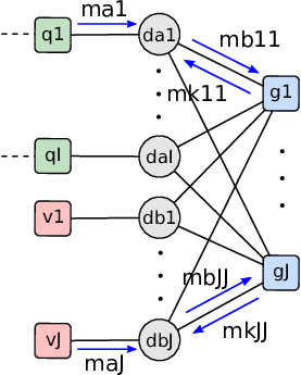
Given factorization (2), a factor graph [25, 28] representing the joint posterior pdf can be constructed. Fig. 1 shows a single time step of this graph.
bp [25, 26, 27, 28] performs local operations on factor graphs to compute representations of marginal posterior pdf, called “beliefs”. Since the factor graph in Fig. 1 has loops, the beliefs provided by bp are approximations of the true marginal posteriors , and there are many possible message passing orders [25]. We only send bp messages forward in time and perform iterative message passing at each time step individually [5]. Next, we will present the specific bp messages passed on the graph in Fig
. 1.
III-A Prediction and Birth Messages
First, for each legacy PO , a prediction step is performed to compute the messages that are passed from the factor nodes “” to the variable nodes “”, i.e.,
and . Here, is the predicted probability of object non-existence [5]. For new po , the messages from factor nodes “” to variable nodes “” are simply [25] . In order to ease the notation, we omit the time index in the following and, e.g., simply write instead of .
III-B Iterative Message Passing and Belief Calculation
We now perform iterative message passing between the variable nodes “”, , and the factor nodes “”, . More precisely, at message passing iteration , the messages are passed from the variable nodes “” to the factor nodes “”. For , these messages can be computed according to
| (4) |
and for , we set them to .
Note that, is a normalization factor that ensures .
The messages passed from the factor nodes “” to the variable nodes “” are obtained for as
| (5) |
Here, denotes
marginalization for all except . This marginalization involves integration for continuous random vectors and summation for binary random variables , . Note that our notation indicates that at this point the measurement is already observed and thus fixed.
After the last iteration , the beliefs for all po can be calculated as the normalized product of all incoming messages
according to
| (6) |
Here, again ensures
. The obtained beliefs can then be used for object declaration and state estimation as discussed in
Section II-C.
III-C Approximate Computation of and Complexity
The computation of in (5), relies on a high-dimensional marginalization whose complexity scales exponentially with the number of po . To improve this complexity scaling, we approximate as follows. We interpret as the pdf of and approximate it by a Gaussian pdf via moment matching [23], i.e., . Here, , where is the matched mean and is the matched covariance matrix, i.e., they are equal to the mean and covariance matrix of . As derived in [30], and
are given by
| (7) | ||||
| (8) |
Here, we have
introduced and which use the notation .
In summary, our bp-based tbd algorithm consists of executing the following steps for each time step : First, we perform state prediction according to () for . We then run the iterative message passing scheme by iteratively computing (4) and (7)–(8) for . Finally, after computing the po beliefs according to (6), object declaration and state estimation are performed as described in Section II-C. An inspection of all these computations shows that the operations with the highest complexity are the summations in (7) and (8), whose complexity scales according to . We can therefore conclude that the computational complexity of the proposed algorithm also exhibits this scaling behavior
.
IV Numerical Results
We consider a two-dimensional (2D) simulation scenario with a roi (roi) of . We simulated five objects and 50 time steps. The object states are modeled by random vectors consisting of 2D position , 2D velocity , and the object’s intensity . The objects appear at time steps at positions randomly chosen in the region . The object’s initial velocity is drawn from and the object’s initial intensity is . The object’s position and velocity evolve according to a constant velocity model [31, Ch. 4] with iid (iid) zero-mean Gaussian noise with variance [31, Ch. 4]. The object’s intensity evolves according to a random walk model with iid zero-mean Gaussian noise with variance . The objects disappear at or when they leave the roi.
The measurement is an image of pixels or bins, i.e., . Each bin has a square size with m length, covering the total roi. Pixel , is represented by the 2D vector with center position . We use the measurement model defined by (1) and set the mean and the covariance of the Gaussian random vector to and
| (9) |
respectively. Note that the variance defines the shape of and thus the number of pixels illuminated by object . Furthermore, the covariance of the noise vector in (1) is set to with . These settings lead to a measurement process in which the contribution of object on pixel is large if the intensity of object is large and the position of object is close to pixel .
We employ a particle implementation of our proposed bp-based tbd algorithm denoted by TBD-BP [32, 4]. The spatial pdf of each po state’s belief is represented by 3000 particles. The generation of new pos is based on the measurement , in particular on . To keep the computational complexity low, we initialize a new po only for those pixels whose intensity is larger than the predefined threshold . The spatial pdf of new po is modeled by . Here, is uniform over the area of pixel , is , and is uniform from to . The birth probability of each new po is set to . An object is declared to exist if its existence probability is larger than . We prune po whose existence probability is below and set the survival probability to .
To evaluate the performance of our proposed algorithm, we compute the Euclidean distance based gospa (gospa) metric [33] averaged over 400 simulation runs, with cutoff parameter , order , and . In our first experiment, we compare the proposed TBD-BP with a particle implementation of the mb (mb) filter in [20], referred to as TBD-MB, and the iemb (iemb) filter in [23]. The TBD-IEMB models spatial distributions by Gaussian pdf. The gospa results are displayed in Fig. 2. As the figure shows, TBD-BP with message passing iterations performs slightly better than TBD-BP with , followed by TBD-IEMB, and significantly better than TBD-MB. The lower performance of TBD-MB is due to the fact that it does not model the interaction of objects and tracks them independently. Furthermore, the track initialization scheme of TBD-MB leads to a high number of false tracks resulting in an almost linear increase in gospa for .
In the second experiment, we investigated the GOSPA performance of TBD-BP for different intensity values and variances . As Fig. 3a shows, the gospa error increases for larger . This is due to the fact that for larger , an object illuminates a larger number of neighboring pixels, which in turn leads to more false tracks caused by the now larger number of pixels of higher intensity. Fig. 3b additionally shows that the gospa error decreases as increases
.
V Conclusion
In this letter, we propose a bp method for tracking an unknown number of low-observable objects based on the tbd approach. We introduced a new object birth model and a new measurement model that allows interacting objects to contribute to more than one data cell. To reduce computational complexity and improve scalability, certain bp messages are approximated by Gaussian distributions. Experiments conducted on image data show that the proposed TBD-BP method outperforms two state-of-the-art tbd mb filtering methods [20, 23]. However, the proposed method is limited to measurements that are independent conditioned on the object states. An interesting possibility for future research is the design of a more general measurement model and an application to real data. Other promising directions for future research are the development of tbd approaches for extended object tracking [9] or based on particle flow [34, 35, 36, 37] and an extension to hybrid model-based and data-driven tbd [38].
References
- [1] Y. Bar-Shalom, P. K. Willett, and X. Tian, Tracking and Data Fusion: A Handbook of Algorithms. Storrs, CT: Yaakov Bar-Shalom, 2011.
- [2] R. Mahler, Statistical Multisource-Multitarget Information Fusion. Norwood, MA: Artech House, 2007.
- [3] S. Challa, M. R. Morelande, D. Mušicki, and R. J. Evans, Fundamentals of Object Tracking. Cambridge, UK: Cambridge University Press, 2011.
- [4] F. Meyer, P. Braca, P. Willett, and F. Hlawatsch, “A scalable algorithm for tracking an unknown number of targets using multiple sensors,” IEEE Trans. Signal Process., vol. 65, no. 13, pp. 3478–3493, Jul. 2017.
- [5] F. Meyer, T. Kropfreiter, J. L. Williams, R. Lau, F. Hlawatsch, P. Braca, and M. Z. Win, “Message passing algorithms for scalable multitarget tracking,” Proc. IEEE, vol. 106, no. 2, pp. 221–259, Feb. 2018.
- [6] J. L. Williams, “Marginal multi-Bernoulli filters: RFS derivation of MHT, JIPDA and association-based MeMBer,” IEEE Trans. Aerosp. Electron. Syst., vol. 51, no. 3, pp. 1664–1687, Jul. 2015.
- [7] G. Ferri, A. Munafò, A. Tesei, P. Braca, F. Meyer, K. Pelekanakis, R. Petroccia, J. Alves, C. Strode, and K. LePage, “Cooperative robotic networks for underwater surveillance: an overview,” IET Radar Sonar Navig., vol. 11, no. 12, pp. 1740–1761, Dec. 2017.
- [8] K. Witrisal, P. Meissner, E. Leitinger, Y. Shen, C. Gustafson, F. Tufvesson, K. Haneda, D. Dardari, A. F. Molisch, A. Conti, and M. Z. Win, “High-accuracy localization for assisted living: 5G systems will turn multipath channels from foe to friend,” IEEE Signal Process. Mag., vol. 33, no. 2, pp. 59–70, Mar. 2016.
- [9] F. Meyer and J. L. Williams, “Scalable detection and tracking of geometric extended objects,” IEEE Trans. Signal Process., vol. 69, pp. 6283–6298, Oct. 2021.
- [10] S. Tonissen and Y. Bar-Shalom, “Maximum likelihood track-before-detect with fluctuating target amplitude,” IEEE Trans. Aerosp. Electron. Syst., vol. 34, no. 3, pp. 796–809, Jul. 1998.
- [11] L. R. Moyer, J. Spak, and P. Lamanna, “A multi-dimensional Hough transform-based track-before-detect technique for detecting weak targets in strong clutter backgrounds,” IEEE Trans. Aerosp. Electron. Syst., vol. 47, no. 4, pp. 3062–3068, Oct. 2011.
- [12] Y. Barniv, “Dynamic programming solution for detecting dim moving targets,” IEEE Trans. Aerosp. Electron. Syst., vol. 21, no. 1, pp. 144–156, Jan. 1995.
- [13] D. Salmond and H. Birch, “A particle filter for track-before-detect,” in Proc. ACC-01, Jun. 2001, pp. 3755–3760.
- [14] M. Orton and W. Fitzgerald, “A Bayesian approach to tracking multiple targets using sensor arrays and particle filters,” vol. 50, no. 2, pp. 216–223, Feb. 2002.
- [15] Y. Boers, J. N. Driessen, F. Verschure, W. P. M. H. Heemels, and A. Juloski, “A multi target track before detect application,” in Proc. CVPRW-03, Jun. 2003, pp. 104–104.
- [16] N. Ito and S. Godsill, “A multi-target track-before-detect particle filter using superpositional data in non-Gaussian noise,” vol. 27, pp. 1075–1079, Jun. 2020.
- [17] S. J. Davey and H. X. Gaetjens, Track-Before-Detect Using Expectation Maximisation. Singapore: Springer, 2018.
- [18] B. Ristic, B.-T. Vo, B.-N. Vo, and A. Farina, “A tutorial on Bernoulli filters: Theory, implementation and applications,” IEEE Trans. Signal Process., vol. 61, no. 13, pp. 3406–3430, Apr. 2013.
- [19] B. Ristic, L. Rosenberg, D. Y. Kim, X. Wang, and J. Williams, “Bernoulli track-before-detect filter for maritime radar,” IET Radar, Sonar Navig., vol. 14, no. 3, pp. 356–363, Mar. 2020.
- [20] B.-N. Vo, B.-T. Vo, N.-T. Pham, and D. Suter, “Joint detection and estimation of multiple objects from image observations,” IEEE Trans. Signal Process., vol. 58, no. 10, pp. 5129–5141, Oct. 2010.
- [21] T. Kropfreiter, J. L. Williams, and F. Meyer, “A scalable track-before-detect method with Poisson/multi-Bernoulli model,” in Proc. FUSION-21, Nov. 2021, pp. 1–8.
- [22] D. Y. Kim, B. Ristic, R. Guan, and L. Rosenberg, “A Bernoulli track-before-detect filter for interacting targets in maritime radar,” IEEE Trans. Aerosp. Electron. Syst., vol. 57, no. 3, pp. 1981–1991, Jun. 2021.
- [23] E. S. Davies and Á. F. García-Fernández, “A multi-Bernoulli Gaussian filter for track-before-detect with superpositional sensors,” in Proc. FUSION-22, Jul. 2022, pp. 1–8.
- [24] C. Cao and Y. Zhao, “A generalized labeled multi-Bernoulli filter based on track-before-detect measurement model for multiple-weak-target state estimate using belief propagation,” Remote Sensing, vol. 14, no. 17, pp. 1–18, Aug. 2022.
- [25] F. R. Kschischang, B. J. Frey, and H.-A. Loeliger, “Factor graphs and the sum-product algorithm,” IEEE Trans. Inf. Theory, vol. 47, no. 2, pp. 498–519, Feb. 2001.
- [26] J. Yedidia, W. Freemand, and Y. Weiss, “Constructing free-energy approximations and generalized belief propagation algorithms,” IEEE Trans. Inf. Theory, vol. 51, no. 7, pp. 2282–2312, July 2005.
- [27] D. Koller and N. Friedman, Probabilistic Graphical Models: Principles and Techniques. Cambridge, MA: MIT Press, 2009.
- [28] H.-A. Loeliger, “An introduction to factor graphs,” IEEE Signal Process. Mag., vol. 21, no. 1, pp. 28–41, Jan. 2004.
- [29] H. V. Poor, An Introduction to Signal Detection and Estimation, 2nd ed. New York: Springer-Verlag, 1994.
- [30] M. Liang, T. Kropfreiter, and F. Meyer, “A BP method for track-before-detect: Supporting derivations,” 2023, https://fmeyer.ucsd.edu/SPL-2023-SD.pdf.
- [31] Y. Bar-Shalom, T. Kirubarajan, and X.-R. Li, Estimation with Applications to Tracking and Navigation. New York, NY: Wiley, 2002.
- [32] A. Ihler and D. McAllester, “Particle belief propagation,” in Proc. AISTATS-09, vol. 5, Apr. 2009, pp. 256–263.
- [33] A. S. Rahmathullah, Á. F. García-Fernández, and L. Svensson, “Generalized optimal sub-pattern assignment metric,” in Proc. FUSION-17, Jul. 2017, pp. 1–8.
- [34] F. Daum and J. Huang, “Nonlinear filters with log-homotopy,” in Proc. SPIE-07, Aug. 2007, pp. 423–437.
- [35] J. Jang, F. Meyer, E. R. Snyder, S. M. Wiggins, S. Baumann-Pickering, and J. A. Hildebrand, “Bayesian detection and tracking of odontocetes in 3-D from their echolocation clicks,” J. Acoust. Soc. Am., vol. 153, no. 5, pp. 2690–2705, May 2023.
- [36] L. Dai and F. Daum, “On the design of stochastic particle flow filters,” IEEE Trans. Aerosp. Electron. Syst., vol. 59, no. 3, pp. 2439–2450, 2023.
- [37] W. Zhang and F. Meyer, “Multisensor multiobject tracking with high-dimensional object states,” 2023, https://arxiv.org/abs/2212.14556.
- [38] M. Liang and F. Meyer, “Neural enhanced belief propagation for multiobject tracking,” IEEE Trans. Signal Process., 2023, to appear.