跳到论文正文
W Papers独立论文阅读器 arXiv:2307.00575 论文正文 计算阅读时间 · 0%
引用这篇论文根据当前论文元数据生成,正式投稿前建议核对。


License: CC BY-NC-SA 4.0
arXiv:2307.00575v2 [stat.ME] 04 Aug 2024

Mode-wise Principal Subspace Pursuit and Matrix Spiked Covariance Model

Runshi Tang Note: Department of Statistics, University of Wisconsin-Madison    Ming Yuan Note: Department of Statistics, Columbia University       Anru R. Zhang Note: Departments of Biostatistics & Bioinformatics and Computer Science, Duke University
(August 11, 2026)
Abstract

We collect the simulation studies, additional real data analysis on functional MRI of cocaine users, and all technical proofs in these supplementary materials.

1 Introduction

In modern scientific applications, data are often observed in the form of multiple matrices or tensors that pertain to different subjects from a certain population. For instance, longitudinal gene expression data consist of a matrix of gene expression levels across time for each subject (Liu et al., 2017); MRI imaging data contain one order-3 tensor image for each patient (Zhou et al., 2013); multilayer network can be represented by an order-3 tensor, where each layer (i.e., a matrix) represents one network (Jing et al., 2021); mm-uniform hypergraph is typically viewed as an order-mm tensor, whose entries denote all hyper-edges (Zhen and Wang, 2022); atomic-resolution 4D scanning transmission electron microscopy data can be expressed as an order-3 tensor with two models denoting scan location and the other denoting the convergent beam electron diffraction pattern (Zhang et al., 2020). Combining information from all subjects results in a high-order tensor with subject independence along one mode and some covariance structure along the other modes that represent the relationship among the measured covariates.

Principal Component Analysis (PCA) is a widely accepted method for analyzing data consisting of vectors associated with individual subjects. Its primary objective is to identify a lower-dimensional subspace within the feature domain that captures the majority of data variance (Pearson, 1901). PCA is a reliable technique for reducing the dimensionality of data. Singular Value Decomposition (SVD) is an efficient approach commonly used to compute PCA. However, when the dataset is in the form of a series of matrices, PCA encounters challenges.

In the literature, the tensor SVD framework (also known as tensor PCA in the machine learning and information theory community) is discussed (Richard and Montanari, 2014; Zhang and Xia, 2018; Wang and Li, 2020; Zhou et al., 2022; Han et al., 2022b). This framework revolves around a signal-plus-noise model: 𝐘=𝐗+𝐙{\mathbf{Y}}={\mathbf{X}}+{\mathbf{Z}}, where 𝐗{\mathbf{X}} represents a mean tensor with certain low-complexity structures (e.g., CP, Tucker, tubal, tensor-train low-rank, etc.), and 𝐙{\mathbf{Z}} denotes mean-zero random observational noise. The goal of tensor SVD (or tensor PCA) is to efficiently extract 𝐗{\mathbf{X}} from 𝐘{\mathbf{Y}}. However, this approach is not suitable for analyzing high-order covariance structures of tensor data due to several reasons. First, most mean-based SVD methodologies assume that the dataset has some tensor low rankness, but this assumption may not always hold true. Second, tensor SVD or low-rank tensor factorization primarily focuses on the mean structure of the data tensor, simplifying the problem to a significantly lower number of parameters compared to the covariance structure. To fix ideas, consider for instance repeated observations of matrix data. While nn i.i.d. copies of pp-by-pp matrix result in a data tensor with n​p2np^{2} entries, the associated covariance tensor includes p4p^{4} entries. Most importantly, tensor SVD or low-rank tensor factorization (Kolda and Bader, 2009; Zhang and Xia, 2018) may not fit for treating the data tensor as information obtained from independent replicates of a certain population. Consequently, achieving good performance in covariance tensor statistical inference using mean-based models cannot be expected.

Since the direct analysis of the covariance tensor of pp-by-pp observational data matrices involves p4p^{4} parameters and is typically difficult in high-dimensional settings, a number of simplified covariance tensor structures were introduced, including the (approximate) Kronecker product distribution (see, e.g., Dawid, 1981; Dutilleul, 1999; Yin and Li, 2012; Tsiligkaridis and Hero, 2013; Zhou, 2014; Chen and Liu, 2015; Hoff, 2015; Ding and Dennis Cook, 2018; Hoff et al., 2022):

𝚺=Σ1⊗KΣ2,i.e.,𝚺i​j​k​l=(Σ1)i​k⋅(Σ2)j​l,\boldsymbol{\Sigma}=\Sigma_{1}\otimes_{K}\Sigma_{2},\quad\text{i.e.,}\quad\boldsymbol{\Sigma}_{ijkl}=(\Sigma_{1})_{ik}\cdot(\Sigma_{2})_{jl},

and Kronecker sum distribution (Greenewald et al., 2013; Greenewald et al., 2017):

Σ=Σ1⊕KΣ2:=Ip1⊗KΣ2+Σ1⊗KIp2,i.e.,𝚺i​j​k​l=(Σ1)i​k1{j=l}+(Σ2)j​l1{i=k},i,j,k,l=1,…,p,\Sigma=\Sigma_{1}\oplus_{K}\Sigma_{2}:=I_{p_{1}}\otimes_{K}\Sigma_{2}+\Sigma_{1}\otimes_{K}I_{p_{2}},\quad\text{i.e.,}\quad\boldsymbol{\Sigma}_{ijkl}=(\Sigma_{1})_{ik}1_{\{j=l\}}+(\Sigma_{2})_{jl}1_{\{i=k\}},i,j,k,l=1,\ldots,p,

where ⊗K\otimes_{K} denotes the Kronecker product: (A⊗KB)p3​(r−1)+v,p4​(s−1)+w=Ar​s​Bv​w(A\otimes_{K}B)_{p_{3}(r-1)+v,p_{4}(s-1)+w}=A_{rs}B_{vw} for matrices A∈ℝp1,p2A\in\mathbb{R}^{p_{1},p_{2}} and B∈ℝp3,p4B\in\mathbb{R}^{p_{3},p_{4}}. These models simplify the entire covariance tensor into two matrices Σ1\Sigma_{1} and Σ2\Sigma_{2}, which greatly streamline subsequent analysis. Nevertheless, these tensor-to-matrix simplifications can impose certain limitations. Additionally, the simplified covariance tensor fails to discern the direction of covariates with higher variances, unlike the vector-based principal component analysis (PCA) technique. As a consequence, the existing literature does not provide a direct equivalent of PCA specifically designed for tensor data. Therefore, there is a disparity in the current research.

To address this disparity, this paper aims to introduce a novel framework for dimension reduction in a series of matrix data, referred to as Mode-wise Principal Subspace Pursuit (MOP-UP). The primary objective of MOP-UP is to extract concealed variations in both the row and column dimensions of data matrices. Specifically, for a collection of matrix data with a shared dimension, denoted as X1,…,Xn∈ℝp1×p2X_{1},\ldots,X_{n}\in\mathbb{R}^{p_{1}\times p_{2}}, we aim to identify the common column and row subspaces represented by semi-orthogonal matrices11 1 A semi-orthogonal matrix is defined as a matrix with orthonormal columns., U∈ℝp1×r1U\in\mathbb{R}^{p_{1}\times r_{1}} and V∈ℝp2×r2V\in\mathbb{R}^{p_{2}\times r_{2}}, respectively. The objective is to approximate the following decomposition for each matrix XiX_{i}:

Xi≈M+U​Ai+Bi​V⊤,X_{i}\approx M+UA_{i}+B_{i}V^{\top}, (1)

where ii ranges from 1 to nn and AiA_{i} and BiB_{i} are score matrices that vary across the indices. Intuitively, the decomposition (1) captures the row-wise and column-wise dimension-reduced subspaces, denoted by UU and VV respectively, which encompass the majority of the informative features present in XiX_{i}.

1.1 Matrix Spiked Covariance Models and Higher-order Generalizations

To establish a statistical foundation for the MOP-UP framework and to serve as a source of inspiration for algorithmic and theoretical development, it is beneficial to review the conventional probabilistic PCA model (Tipping and Bishop, 1999) before delving deeper. Suppose x1,…,xnx_{1},\ldots,x_{n} are a series of pp-dimensional i.i.d. observations with mean vector μ\mu and covariance matrix Σ\Sigma. The goal of PCA is to seek a few loading vectors that explain most of the variance in data through the following decomposition,

xi=μ+U​ai⊤+zi=μ+∑j=1ruj​ai​j+zi.x_{i}=\mu+Ua_{i}^{\top}+z_{i}=\mu+\sum_{j=1}^{r}u_{j}a_{ij}+z_{i}. (2)

Here U=[u1,…,ur]∈ℝp×rU=[u_{1},\ldots,u_{r}]\in\mathbb{R}^{p\times r} is a set of fixed and uniform orthogonal vectors for all observations, ai​1,…,ai​ra_{i1},\ldots,a_{ir} are random values, ziz_{i} represents the noise. Particularly, UU and aa are often referred to as “loading” and “principal component (PC) scores” in the literature. To theoretically analyze the performance of PCA, the following spiked covariance model was introduced and widely studied (Johnstone, 2001; Paul, 2007; Cai et al., 2013; Donoho et al., 2018; Cai et al., 2016),

Σ=σ2​I+U​Λ​U⊤=σ2​I+∑i=1rλi​ui​ui⊤,U∈𝕆p,r.\Sigma=\sigma^{2}I+U\Lambda U^{\top}=\sigma^{2}I+\sum_{i=1}^{r}\lambda_{i}u_{i}u_{i}^{\top},\quad U\in\mathbb{O}_{p,r}.

An equivalent form of this model can be obtained by algebraic calculation as

(Σ−σ2​I)​U⟂=0,U⟂ is the orthogonal complement of U.(\Sigma-\sigma^{2}I)U_{\perp}=0,\quad\text{$U_{\perp}$ is the orthogonal complement of $U$.} (3)

In the noiseless setting (i.e., σ2=0\sigma^{2}=0), the low-rank property of the data is equivalent to the low-rank property of its covariance matrix, as illustrated by the correspondence between (2) and (3). We aim to extend this connection to the matrix-variate scenario. Suppose 𝐗=[X1,…,Xn]{\mathbf{X}}=[X_{1},\ldots,X_{n}] is an order-3 dataset, where X1,…,XnX_{1},\ldots,X_{n} are i.i.d. matrix observations with mean matrix MM. Now we still seek a low-dimensional row subspace UU and a low-dimensional column subspace VV that can together explain most of the variance in 𝐗{\mathbf{X}}. In analogy to the matrix PCA of (2) and (3), we consider the following two models

Xi=M+UAi⊤+BiV⊤+Zi,i=1,…,n,X_{i}=M+UA_{i}^{\top}+B_{i}V^{\top}+Z_{i},\quad i=1,\ldots,n, (4)
(V⟂⊗KU⟂)⊤​(Cov⁡(vec⁡(X))−σ2​Ip1​p2)=0,for some fixed semi-orthogonal matrices U⟂ and V⟂,(V_{\perp}\otimes_{K}U_{\perp})^{\top}({\rm Cov}({\operatorname{vec}}(X))-\sigma^{2}I_{p_{1}p_{2}})=0,\quad\text{for some fixed semi-orthogonal matrices $U_{\perp}$ and $V_{\perp}$}, (5)

where vec⁡(X){\operatorname{vec}}(X) denotes the vectorization of the matrix XX, formed by stacking the columns of XX into a single column vector. (5) can be equivalently written as

(Cov(X)−σ2𝐈(p1×p2)2)×1U⟂×2V⟂=0,for some fixed semi-orthogonal matrices U⟂ and V⟂.({\rm Cov}(X)-\sigma^{2}{{\mathbf{I}}_{(p_{1}\times p_{2})_{2}}})\times_{1}U_{\perp}\times_{2}V_{\perp}=0,\quad\text{for some fixed semi-orthogonal matrices $U_{\perp}$ and $V_{\perp}$}. (6)

Here, Cov⁡(X)=𝔼⁡((X−𝔼​X)⊗(X−𝔼​X)){\rm Cov}(X)=\mathbb{E}((X-\mathbb{E}X)\otimes(X-\mathbb{E}X)) denote the covariance tensor, ⊗\otimes denotes the tensor product, and ×1\times_{1} and ×2\times_{2} represent the tensor-matrix product, which will be introduced in Section 2.1. The matrices UU and VV are analogous to UU in the regular PCA (2) and can be referred to as the column and row loading matrices, respectively. The matrices AiA_{i} and BiB_{i} are random matrices that correspond to the scores aka_{k} in PCA (2), and can be referred to as score matrices. Additionally, ZiZ_{i} represents the noise involved in the process.

Model (4) provides a rigorous statistical interpretation for the MOP-UP framework. Additionally, Models (4) and (5) (or (6)) correspond to (2) and (3) respectively, which are part of the classical spiked covariance model. Formulations (4) and (5) (or (6)) are proven to be equivalent in the upcoming Theorem 1. Based on this equivalence, this paper introduces and studies the class of matrix spiked covariance models that satisfies either decomposition (4) or condition (5) (or (6)). See Figure 1 for an illustration of matrix spiked covariance model.

Refer to caption
Figure 1: Illustration of a matrix spiked covariance model in a decomposition form

Furthermore, we say 𝐗∈ℝ𝐩{\mathbf{X}}\in\mathbb{R}^{{\mathbf{p}}} has a rank-𝐫{\mathbf{r}} high-order spiked covariance if

𝐗=𝐌+∑k=1d𝐀k×kUk+𝐙,{\mathbf{X}}={\mathbf{M}}+\sum_{k=1}^{d}{\mathbf{A}}_{k}\times_{k}U_{k}+{\mathbf{Z}}, (7)

or equivalently

Cov⁡(𝐗)=𝚺0+σ2​𝐈𝐩,𝚺0∈ℝ𝐩×𝐩,𝚺0×k=1dUk⟂=0.{\rm Cov}({\mathbf{X}})=\boldsymbol{\Sigma}_{0}+\sigma^{2}{{\mathbf{I}}_{{\mathbf{p}}}},\ \boldsymbol{\Sigma}_{0}\in\mathbb{R}^{{\mathbf{p}}\times{\mathbf{p}}},\ \boldsymbol{\Sigma}_{0}\times_{k=1}^{d}U_{k\perp}=0. (8)

Here, 𝐩=p1×⋯×pd{\mathbf{p}}=p_{1}\times\cdots\times p_{d}, 𝐌∈ℝ𝐩{\mathbf{M}}\in\mathbb{R}^{{\mathbf{p}}} is a fixed mean tensor, Uk∈𝕆pk,rkU_{k}\in\mathbb{O}_{p_{k},r_{k}} are fixed semi-orthogonal matrices, 𝐀k∈ℝp1×⋯×pk−1×rk×pk+1×⋯×pd{\mathbf{A}}_{k}\in\mathbb{R}^{p_{1}\times\cdots\times p_{k-1}\times r_{k}\times p_{k+1}\times\cdots\times p_{d}} are random tensors with mean zero, and 𝐙∈ℝ𝐩{\mathbf{Z}}\in\mathbb{R}^{{\mathbf{p}}} is a noise tensor, where all entries of 𝐙{\mathbf{Z}} has mean zero, covariance σ2​𝐈𝐩\sigma^{2}{\mathbf{I}}_{{\mathbf{p}}}, and is uncorrelated with random tensors 𝐀1,…,𝐀d{\mathbf{A}}_{1},\ldots,{\mathbf{A}}_{d}. 𝐈𝐩{\mathbf{I}}_{\mathbf{p}} is the order-(2​d)(2d) tensor in ℝ𝐩×𝐩\mathbb{R}^{\mathbf{p}\times\mathbf{p}} with entries (𝐈𝐩)𝐪,𝐪=1({\mathbf{I}}_{\mathbf{p}})_{\mathbf{q},\mathbf{q}}=1 and 𝐪=(q1,q2,⋯,qd)\mathbf{q}=(q_{1},q_{2},\cdots,q_{d}), qk∈{1,⋯,pk}q_{k}\in\{1,\cdots,p_{k}\}, and 0 elsewhere. (7) and (8) can be viewed as generalization of (4) and (5) (or (6)), respectively, and their equivalence will be discussed in Theorem 8.

In summary, the proposed matrix and higher-order spiked covariance models relax the restrictive assumptions (such as the Kronecker product and sum) while still allowing a large number of free variables in the covariance tensor 𝚺\boldsymbol{\Sigma}.

1.2 Our Contributions

We present the Mode-wise Principal Subspace Pursuit (MOP-UP) framework, designed to uncover concealed variations in both the row and column dimensions of data matrices. MOP-UP is supported by a novel class of matrix-variate spiked covariance models, representing a significant generalization beyond the traditional vector-case spiked covariance model. The decomposition formula (4) we introduce offers enhanced flexibility compared to existing dimension reduction formulations in the literature, enabling effective decomposition of a series of matrices. Our framework also extends the spiked covariance model to accommodate matrix and higher-order tensor samples, broadening its applicability from a statistical perspective.

To address dimension reduction for data matrices adhering to the POP-UP framework and the matrix spiked covariance model, we propose two novel methods: Average Subspace Capture (ASC) and Alternating Projection (AP). The ASC method introduces a new average projector estimator, distinct from the commonly used spectral initialization method found in existing literature. We highlight the geometric interpretations of ASC and provide theoretical guarantees that it achieves precise recovery of singular spaces almost sure in the noiseless scenarios. In contrast, our AP iteration procedure significantly deviates from the prevailing class of power iteration algorithms seen in the literature. We establish that AP essentially performs alternating minimization for an objective function that can be readily interpreted. Furthermore, we derive a statistical upper bound on the estimation error for ASC, AP, as well as their combined usage, providing valuable insights into their performance.

We also study the methods and theory for higher-order spiked covariance models. Our investigation reveals notable differences in the algorithmic procedures for the spiked covariance model across various cases, including vector-variate, matrix-variate, and higher-order-variate scenarios. To provide a comprehensive overview, we summarize a comparison of the decomposition procedures for these different variate cases in Table 1.

Table 1: Comparison of procedures for spiked models in different variate cases
Vector case Matrix case Higher-order tensor case
Initialization SVD Average Subspace Capture (ASC) HOSVD
Followup iteration? No
No (noiseless case)
Yes (noisy case)
Yes

To validate the efficacy of our model, we conduct data experiments on both synthetic and real-world datasets. First, we do simulation studies to show the tightness of our error bounds. Second, we apply the MOP-UP method to preprocess the MNIST dataset, reducing the dimensionality of the digit images before training a classifier. This approach yields interpretable dimension-reduced image features and demonstrated accurate prediction accuracy in the testing set when compared to traditional tensor methods. Third, we utilize the MOP-UP method on a human brain fMRI dataset obtained from a clinical study on cocaine use. Our results clearly demonstrate the effectiveness of our framework in preprocessing the data for the classification of cocaine and non-cocaine users, as well as for clustering region of interest (ROI) tasks. In both cases, our method showcases notable advantages in terms of the best prediction measurement and robustness across different input hyperparameters.

Furthermore, we introduce a new technical tool of a matrix perturbation bound, which greatly aids in the technical analysis of the proposed MOP-UP. Our innovative methodology focuses on deriving a blockwise eigenspace perturbation bound, enabling us to establish our primary result with precision. This approach holds substantial value not only in situations where classical perturbation bounds, such as Davis-Kahan’s theorem, may fall short in accurately assessing errors but also in other scenarios. Its applicability extends beyond the immediate context of our proposed MOP-UP, making it of independent interest.

1.3 Literature Review

In this section, we provide a brief overview of the related literature in the field. Principal Component Analysis (PCA) is one of the most well-established dimensionality reduction techniques, and numerous variations and related methods have been extensively studied. Textbooks such as Jolliffe, 2005; Abdi and Williams, 2010 offer comprehensive coverage of PCA and its variants, including factor analysis, independent component analysis, and projection pursuit. Several studies have investigated the distribution of eigenvalues in PCA under various assumptions. For example, Johnstone, 2001 examined the distribution of the largest eigenvalue in PCA when the covariance matrix is an identity matrix under Gaussianity. Paul, 2007 analyzed the eigenvalue distribution assuming Gaussianity and a specific covariance matrix structure. Shrinkage methods for eigenvalue regularization were studied by Donoho et al., 2018 under more general settings. Asymptotic properties of eigenvalues and eigenvectors were explored by Bao et al., 2022. Extensions of PCA to matrices and images have also been investigated. Matrix PCA or 2-D PCA methods were developed to analyze matrix objects and images (Ye et al., 2004; Ye, 2004a). Yang et al., 2004 considered applying linear transformations to the right side of observed matrices, while Ye et al., 2004 proposed an algorithm that incorporated spatial correlation of image pixels and applied linear transformations to both the left and right sides of observed matrices. He et al., 2005 introduced the tensor subspace analysis algorithm, which treats input images as matrices residing in a tensor space and detects local geometric structures within that space. Furthermore, studies by Koltchinskii and Lounici, 2016; Koltchinskii and Lounici, 2017; Koltchinskii et al., 2020 have focused on the spectral distribution of sample covariance matrices. Zhang et al., 2022 proposed HeteroPCA, a variation of PCA that accounts for heteroskedasticity in the data. Efron, 2009 considered a matrix XX whose rows are possibly correlated and aimed to test the hypothesis that the columns are independent of each other. He found that the row and column correlations of XX interact with each other in a way that complicates test procedures, essentially by reducing the accuracy of the relevant estimators. In contrast, our paper explores distinct problems, focusing on reducing multiple data matrices to dimension-reduced row and column subspaces.

PCA relies on the mathematical tool of Singular Value Decomposition (SVD), which is a widely used matrix decomposition method. In recent years, SVD has been extended to tensor objects, leading to various generalizations such as Canonical Polyadic (CP) decomposition (Anandkumar et al., 2014; Ouyang and Yuan, 2023), tensor train (Zhou et al., 2022), and Tucker decomposition (Hitchcock, 1927). To find the best low Tucker rank approximation of a given tensor, De Lathauwer et al., 2000a introduced Higher Order Singular Value Decomposition (HOSVD), and De Lathauwer et al., 2000b introduced an alternating least squares algorithm known as High Order Orthogonal Iteration (HOOI). HOOI iteratively projects the tensor into a lower-dimensional space along each mode. The statistical modeling and performance analysis of HOOI were explored in Zhang and Xia, 2018. However, these previous works focused on decomposing a single tensor without considering multiple samples from different subjects. The most relevant paper to our work is Lu et al., 2008, which addressed this limitation by generalizing HOOI to handle multiple tensor observations. Their method, called Multilinear Principal Component Analysis (MPCA), extended the framework to incorporate multiple tensors. Several variations of MPCA have been proposed, including a TTP-based MSL algorithm (Tao et al., 2008), robust MPCA (Inoue et al., 2009), nonnegative MPCA (Panagakis et al., 2009), and others. A survey by Lu et al., 2011 provides a comprehensive summary of methods in this field, including these variations and techniques.

These developments in PCA, SVD, and tensor decomposition methods have partly inspired the framework and algorithms proposed in our work.

1.4 Organization

The remainder of this paper is organized as follows. In Section 2, we provide notation, preliminaries, and a detailed discussion of the matrix spiked covariance model. We then introduce our algorithm in Section 3 and discuss its interpretation in Section 3.2. We compare our model and algorithm to other methods in Section 3.3. The theoretical properties of the algorithms are developed in Section 4. Specifically in Section 4.4, we introduce a technical lemma, a blockwise eigenspace perturbation bound, which plays a key role in our analysis. Furthermore, we present real data experiments in Section 5. Finally, we discuss the generalization to higher-order tensor cases and summarise our results in Section 6. Simulation studies, additional real data analyses, and all technical proofs are collected in the Supplementary Materials.

2 Models

2.1 Notation and Preliminaries

In this work, lowercase letters (u,v,μu,v,\mu, etc.) represent scalars or vectors; uppercase letters (A,B,UA,B,U, etc.) represent matrices; and bold uppercase letters (𝐗,𝐙{\mathbf{X}},{\mathbf{Z}}, etc.) represent tensors. For variables xx and yy, x≲yx\lesssim y represents that there exists some constant cc that does not depend on xx or yy such that x≤c​yx\leq cy. For a vector aa, ‖a‖\|a\| denotes its l2l_{2} norm. Let II be the identity matrix with an appropriate dimension based on the context. For a matrix A∈ℝp×qA\in\mathbb{R}^{p\times q}, vec⁡(A)∈ℝp​q{\operatorname{vec}}(A)\in\mathbb{R}^{pq} denotes the vectorization of the matrix AA, formed by stacking the columns of AA into a single vector. σi​(A)\sigma_{i}(A) represents the iith singular value of AA, and all the singular values are ordered by its magnitude: σ1​(A)≥σ2​(A)≥⋯≥σmin⁡{p,q}≥0\sigma_{1}(A)\geq\sigma_{2}(A)\geq\cdots\geq\sigma_{\min\{p,q\}}\geq 0; SVDr​(A)=[u1,⋯,ur]{\rm SVD}_{r}(A)=[u_{1},\cdots,u_{r}] represents the matrix consisting of the top rr left singular vectors of AA, where uiu_{i} is the singular vector of matrix AA corresponding to the singular value σi​(A)\sigma_{i}(A); PA=A​(A⊤​A)†​AP_{A}=A(A^{\top}A)^{\dagger}A denotes an orthogonal projection matrix onto its column space, where (⋅)†(\cdot)^{\dagger} is the matrix pseudo-inverse; ‖A‖\|A\| is the spectral norm of AA, which is equal to its largest singular value, σ1​(A)\sigma_{1}(A); ‖A‖F=tr⁡(A​A⊤)\|A\|_{F}=\sqrt{{\rm tr}(AA^{\top})} is the Frobenius norm of AA.

The kernel (null space) of AA is denoted as ker​(A)={v:A​v=0}\text{ker}(A)=\{v:Av=0\}. The linear space spanned by all columns of AA is denoted as Span​(A)={v=A​w:w∈ℝp}\text{Span}(A)=\{v=Aw:w\in\mathbb{R}^{p}\}. The sum of two linear spaces 𝒱\mathcal{V} and 𝒲\mathcal{W} is represented as 𝒱+𝒲={u=v+w:v∈𝒱,w∈𝒲}\mathcal{V}+\mathcal{W}=\{u=v+w:v\in\mathcal{V},w\in\mathcal{W}\}. We define A​𝒱={A​v:v∈𝒱}A\mathcal{V}=\{Av:v\in\mathcal{V}\} as the range of AA constrained to 𝒱\mathcal{V}. When AA is symmetric with dimensions p=qp=q, λr​(A)\lambda_{r}(A) represents its rrth eigenvalue, ordered such that λ1≥⋯≥λp\lambda_{1}\geq\cdots\geq\lambda_{p}, and Eigenr​(A)=[u1,⋯,u2]{\rm Eigen}_{r}(A)=[u_{1},\cdots,u_{2}] represents the matrix consisting of the top rr eigenvectors of AA. Notice when AA is positive semi-definite, we have Eigenr​(A)=SVDr​(A){\rm Eigen}_{r}(A)={\rm SVD}_{r}(A). For matrices A∈ℝp1,p2A\in\mathbb{R}^{p_{1},p_{2}} and B∈ℝp3,p4B\in\mathbb{R}^{p_{3},p_{4}}, A⊗KB∈ℝp1​p3×p2​p4A\otimes_{K}B\in\mathbb{R}^{p_{1}p_{3}\times p_{2}p_{4}} denotes their Kronecker product, which is defined element-wise as (A⊗KB)p3​(r−1)+v,p4​(s−1)+w=Ar​s​Bv​w(A\otimes_{K}B)_{p_{3}(r-1)+v,p_{4}(s-1)+w}=A_{rs}B_{vw} for r∈{1,⋯,p1},s∈{1,⋯,p2},v∈{1,⋯,p3}r\in\{1,\cdots,p_{1}\},s\in\{1,\cdots,p_{2}\},v\in\{1,\cdots,p_{3}\} and w∈{1,⋯,p4}w\in\{1,\cdots,p_{4}\}. We denote 𝕆p,r:={U∈ℝp×r:U⊤​U=I}\mathbb{O}_{p,r}:=\left\{{U}\in\mathbb{R}^{p\times r}:{U}^{\top}{U}={I}\right\} as the set of all pp-by-rr semi-orthonormal matrices, i.e., matrices with orthonormal columns. For U∈𝕆p,rU\in\mathbb{O}_{p,r}, U⟂U_{\perp} represents a matrix in 𝕆p,p−r\mathbb{O}_{p,p-r} whose columns are orthogonal to the columns of UU. In this work, we employ the sin⁡Θ\sin\Theta distance to characterize the distance between subspaces. For any U,V∈𝕆p,rU,V\in\mathbb{O}_{p,r}, we define ‖sin⁡Θ⁡(U,V)‖=‖U⟂⊤​V‖=‖U​U⊤−V​V⊤‖\|\sin\Theta(U,V)\|=\|U_{\perp}^{\top}V\|=\|UU^{\top}-VV^{\top}\|.

An order-dd tensor 𝐀∈ℝp1×⋯×pd{\mathbf{A}}\in\mathbb{R}^{p_{1}\times\cdots\times p_{d}} can be viewed as a multidimensional array, where (i1,⋯,id)(i_{1},\cdots,i_{d}) maps to 𝐀i1,⋯,id∈ℝ{\mathbf{A}}_{i_{1},\cdots,i_{d}}\in\mathbb{R}. For convenience, we define 𝐩=p1×⋯×pd{\mathbf{p}}=p_{1}\times\cdots\times p_{d}. For a matrix B∈ℝpk×rkB\in\mathbb{R}^{p_{k}\times r_{k}}, the mode-kk product of tensor 𝐀{\mathbf{A}} by matrix BB is denoted as 𝐀×kB∈ℝp1×⋯×pk−1×rk×pk+1×⋯×pd{\mathbf{A}}\times_{k}B\in\mathbb{R}^{p_{1}\times\cdots\times p_{k-1}\times r_{k}\times p_{k+1}\times\cdots\times p_{d}} and defined as (𝐀×kB)i1,⋯,id=∑j=1pk𝐀i1⋯ik−1jik+1⋯idBik​j({\mathbf{A}}\times_{k}B)_{i_{1},\cdots,i_{d}}=\sum_{j=1}^{p_{k}}{\mathbf{A}}_{i_{1}\cdots i_{k-1}ji_{k+1}\cdots i_{d}}B_{i_{k}j}. The mode-kk unfolding of tensor 𝐀{\mathbf{A}} is denoted as ℳk​(𝐀)∈ℝpk×p−k\mathcal{M}_{k}({\mathbf{A}})\in\mathbb{R}^{p_{k}\times p_{-k}} and defined as (ℳk(𝐀))ik,h=𝐀i1⋯id(\mathcal{M}_{k}({\mathbf{A}}))_{i_{k},h}={\mathbf{A}}_{i_{1}\cdots i_{d}}, where h=i1+p1​(i2−1)+⋯+∏j=1k−1pj​(ik+1−1)+pk+1​∏j=1k−1pj​(ik+2−1)+⋯+∏j≠k,j≤d−1pj​(id−1)h=i_{1}+p_{1}(i_{2}-1)+\cdots+\prod_{j=1}^{k-1}p_{j}(i_{k+1}-1)+p_{k+1}\prod_{j=1}^{k-1}p_{j}(i_{k+2}-1)+\cdots+\prod_{j\neq k,j\leq d-1}p_{j}(i_{d}-1). When referring to a random tensor 𝐗{\mathbf{X}}, 𝐗i{{\mathbf{X}}_{i}} denotes its i.i.d. samples. If the random tensor already has a sub-index (e.g., 𝐀k{\mathbf{A}}_{k}), a comma is used to separate the sample index and its original sub-index (e.g., 𝐀i,k{\mathbf{A}}_{i,k}). For two tensors 𝐀∈ℝp1×⋯×pd{\mathbf{A}}\in\mathbb{R}^{p_{1}\times\cdots\times p_{d}} and 𝐁∈ℝq1×⋯×qk{\mathbf{B}}\in\mathbb{R}^{q_{1}\times\cdots\times q_{k}}, the operation 𝐀⊗𝐁∈ℝ𝐩×𝕢{\mathbf{A}}\otimes{\mathbf{B}}\in\mathbb{R}^{{\mathbf{p}}\times\mathbb{q}} denotes the tensor product and (𝐀⊗𝐁)(i1,⋯,id,j1,⋯,jk)=𝐀(i1,⋯,id)​𝐁(j1,⋯,jk)({\mathbf{A}}\otimes{\mathbf{B}})_{(i_{1},\cdots,i_{d},j_{1},\cdots,j_{k})}={\mathbf{A}}_{(i_{1},\cdots,i_{d})}{\mathbf{B}}_{(j_{1},\cdots,j_{k})}. The tensor product “⊗\otimes” should not be confused with the Kronecker product “⊗K\otimes_{K}”, which was defined earlier. The covariance tensor Cov⁡(𝐗){\rm Cov}({\mathbf{X}}) of random tensor 𝐗∈ℝp1×⋯×pd{\mathbf{X}}\in\mathbb{R}^{p_{1}\times\cdots\times p_{d}} is defined as Cov⁡(𝐗)=𝔼⁡((𝐗−𝔼​𝐗)⊗(𝐗−𝔼​𝐗)){\rm Cov}({\mathbf{X}})=\mathbb{E}(({\mathbf{X}}-\mathbb{E}{\mathbf{X}})\otimes({\mathbf{X}}-\mathbb{E}{\mathbf{X}})), i.e., Cov​(𝐗)(i1,⋯,id,j1,⋯,jd)=𝔼⁡[(𝐗−𝔼​𝐗)(i1,⋯,id)​(𝐗−𝔼​𝐗)(j1,⋯,jd)]{\rm Cov}({\mathbf{X}})_{(i_{1},\cdots,i_{d},j_{1},\cdots,j_{d})}=\mathbb{E}[({\mathbf{X}}-\mathbb{E}{\mathbf{X}})_{(i_{1},\cdots,i_{d})}({\mathbf{X}}-\mathbb{E}{\mathbf{X}})_{(j_{1},\cdots,j_{d})}]. When xx is a random vector, Cov⁡(x){\rm Cov}(x) is the covariance matrix. The symbol 𝐈𝐩d{\mathbf{I}}_{\mathbf{p}^{d}} represents an order-(2​d)(2d) tensor in ℝ𝐩×𝐩\mathbb{R}^{\mathbf{p}\times\mathbf{p}} with entries (𝐈𝐩d)𝐪,𝐪=1({\mathbf{I}}_{\mathbf{p}_{d}})_{\mathbf{q},\mathbf{q}}=1, where 𝐪=(q1,q2,⋯,qd)\mathbf{q}=(q_{1},q_{2},\cdots,q_{d}), qk∈{1,⋯,pk}q_{k}\in\{1,\cdots,p_{k}\}, and 0 elsewhere. The symbol 𝐈(p1×p2)2{\mathbf{I}}_{(p_{1}\times p_{2})_{2}} represents an order-44 tensor in ℝp1×p2×p1×p2\mathbb{R}^{p_{1}\times p_{2}\times p_{1}\times p_{2}} with entries (𝐈(p1×p2)2)𝐪,𝐪=1({\mathbf{I}}_{(p_{1}\times p_{2})_{2}})_{\mathbf{q},\mathbf{q}}=1, where 𝐪=(q1,q2)\mathbf{q}=(q_{1},q_{2}), q1∈{1,⋯,p1},q2∈{1,⋯,p2}q_{1}\in\{1,\cdots,p_{1}\},q_{2}\in\{1,\cdots,p_{2}\}, and 0 elsewhere.

We summarise notations in Table 2, and any additional notation will be introduced and defined when they are first used.

Notation
vec⁡(A){\operatorname{vec}}(A) Vectorization of matrix AA by stacking the columns
‖A‖\|A\| Operator norm of matrix AA
‖A‖F\|A\|_{F} Frobenius norm of matrix AA
σi​(A)\sigma_{i}(A) iith singular value of matrix AA
λi​(A)\lambda_{i}(A) iith eigenvalue of symmetric matrix AA
SVDi​(A){\rm SVD}_{i}(A) Matrix of top ii left singular vectors of matrix AA
Eigeni​(A){\rm Eigen}_{i}(A) Matrix of top ii eigenvectors of symmetric matrix AA
span⁡(A)\operatorname{span}(A) Linear span (range) of matrix AA
ker⁡(A)\ker(A) Kernel (null space) of matrix AA
PAP_{A} Orthogonal projection matrix onto column space of matrix AA
U⟂U_{\perp} Orthonormal complement to semi-orthonormal matrix UU
‖sin⁡Θ⁡(U,V)‖\|\sin\Theta(U,V)\| Sine theta distance between semi-orthonormal matrices UU and VV
A⊗KBA\otimes_{K}B Kronecker product of matrix AA and matrix BB
A⊕KBA\oplus_{K}B Kronecker sum of matrix AA and matrix BB
A​𝒱A\mathcal{V} Range of matrix A constrained to linear space 𝒱\mathcal{V}
𝒱+𝒲\mathcal{V}+\mathcal{W} Sum of linear space 𝒱\mathcal{V} and linear space 𝒲\mathcal{W}
𝕆p,r\mathbb{O}_{p,r} Space of pp-by-rr semi-orthonormal matrices
𝐗⊗𝐘{\mathbf{X}}\otimes{\mathbf{Y}} Tensor product of tensor 𝐗{\mathbf{X}} and tensor 𝐘{\mathbf{Y}}
𝐀×kB{\mathbf{A}}\times_{k}B mode-k product of tensor 𝐀{\mathbf{A}} by matrix BB
ℳk​(𝐀)\mathcal{M}_{k}({\mathbf{A}}) mode-kk unfolding of tensor 𝐀{\mathbf{A}}
Cov⁡(𝐗){\rm Cov}({\mathbf{X}}) Covariance tensor of random tensor 𝐗{\mathbf{X}}
𝐈𝐩d{\mathbf{I}}_{\mathbf{p}_{d}} A tensor with entries (𝐈𝐩d)𝐪,𝐪=1({\mathbf{I}}_{\mathbf{p}_{d}})_{\mathbf{q},\mathbf{q}}=1, where 𝐪=(q1,q2,⋯,qd)\mathbf{q}=(q_{1},q_{2},\cdots,q_{d}), and 0 elsewhere
Table 2: Notations. See detailed explanation in Section 2.1.

2.2 Matrix Spiked Covariance Model

We formally introduce the following matrix spiked covariance model as follows.

Definition 1 (High-order Spiked Covariance Model Matrix Variate Case).

Suppose X∈ℝp1×p2X\in\mathbb{R}^{p_{1}\times p_{2}} is a random matrix. We say XX has a rank-(r1,r2)(r_{1},r_{2}) high-order spiked covariance, if there exists σ2>0\sigma^{2}>0, U∈𝕆p1,r1U\in\mathbb{O}_{p_{1},r_{1}}, and V∈𝕆p2,r2V\in\mathbb{O}_{p_{2},r_{2}}, such that

Cov⁡(vec⁡(X))=𝔼​(vec⁡(X)−𝔼​vec⁡(X))⊤​(vec⁡(X)−𝔼​vec⁡(X))=Σ0+σ2​Ip1​p2,Σ0∈ℝp1​p2×p1​p2,{\rm Cov}({\operatorname{vec}}(X))=\mathbb{E}({\operatorname{vec}}(X)-\mathbb{E}{\operatorname{vec}}(X))^{\top}({\operatorname{vec}}(X)-\mathbb{E}{\operatorname{vec}}(X))=\Sigma_{0}+\sigma^{2}I_{p_{1}p_{2}},\ \Sigma_{0}\in\mathbb{R}^{p_{1}p_{2}\times p_{1}p_{2}},
(V⟂⊗KU⟂)⊤​Σ0=0;(V_{\perp}\otimes_{K}U_{\perp})^{\top}\Sigma_{0}=0;

or equivalently, with tensor notations,

Cov(X)=𝔼((X−𝔼X)⊗(X−𝔼X))=𝚺0+σ2𝐈(p1×p2)2,𝚺0∈ℝp1×p2×p1×p2,𝚺0×1U⟂×2V⟂=0.{\rm Cov}(X)=\mathbb{E}\left((X-\mathbb{E}X)\otimes(X-\mathbb{E}X)\right)=\boldsymbol{\Sigma}_{0}+\sigma^{2}{{\mathbf{I}}_{(p_{1}\times p_{2})_{2}}},\ \boldsymbol{\Sigma}_{0}\in\mathbb{R}^{p_{1}\times p_{2}\times p_{1}\times p_{2}},\quad\boldsymbol{\Sigma}_{0}\times_{1}U_{\perp}\times_{2}V_{\perp}=0.

To ensure the existence of U⟂U_{\perp} and V⟂V_{\perp}, we always assume pi>rip_{i}>r_{i} for all ii in this work. The following theorem shows that the high-order spiked covariance model can be equivalently written as a decomposition form (9) as depicted in Figure 1.

Theorem 1 (Equivalent Definitions for High-order Spiked Covariance).

X∈ℝp1×p2X\in\mathbb{R}^{p_{1}\times p_{2}} satisfies the high-order spiked covariance model if and only if there exist a deterministic matrix MM, random matrices B∈ℝp1×r2B\in\mathbb{R}^{p_{1}\times r_{2}} and A∈ℝr1×p2A\in\mathbb{R}^{r_{1}\times p_{2}} with mean 0 such that

X=M+U​A+B​V⊤+Z.X=M+UA+BV^{\top}+Z. (9)

Here, U∈𝕆p1,r1,V∈𝕆p2,r2U\in\mathbb{O}_{p_{1},r_{1}},V\in\mathbb{O}_{p_{2},r_{2}} are fixed semi-orthogonal matrices, Z∈ℝp1×p2Z\in\mathbb{R}^{p_{1}\times p_{2}} is a random matrix, where all entries of ZZ are independent with mean zero and covariance σ2\sigma^{2}, and are uncorrelated with A,BA,B.

The question of identifiability is particularly important: if a population covariance tensor Cov​(X)\text{Cov}(X) satisfies a high-order spiked covariance model (i.e., (9) holds), when can the subspaces span⁡(U)\operatorname{span}(U) and span⁡(V)\operatorname{span}(V) be uniquely identified based on XX? The following theorem provides a mild sufficient condition for identifiability.

Theorem 2 (Identifiability Condition for Matrix Spiked Covariance Model).

Suppose Y=U​A+B​V⊤Y=UA+BV^{\top}, where U∈𝕆p1,r1,V∈𝕆p2,r2U\in\mathbb{O}_{p_{1},r_{1}},V\in\mathbb{O}_{p_{2},r_{2}} are deterministic matrices and A∈ℝr1×p2,B∈ℝp1×r2A\in\mathbb{R}^{r_{1}\times p_{2}},B\in\mathbb{R}^{p_{1}\times r_{2}} are random matrices. Suppose for any nonzero v∈ℝp2v\in\mathbb{R}^{p_{2}} and any affine subspace (In this work, affine subspace refers to {v+e1u1+⋯+erur:e1,…,er∈ℝ}\{v+e_{1}u_{1}+\cdots+e_{r}u_{r}:e_{1},\ldots,e_{r}\in\mathbb{R}\}, where v,u1,…,urv,u_{1},\ldots,u_{r} are all vectors of the same dimension.) 𝒲⊆ℝp1\mathcal{W}\subseteq\mathbb{R}^{p_{1}}, either ℙ⁡(U​A​v∈𝒲|B)<1\mathbb{P}\left(UAv\in\mathcal{W}|B\right)<1 or span⁡(U)⊆𝒲\operatorname{span}(U)\subseteq\mathcal{W}. Then, UU is identifiable in the sense that for any fixed U′∈𝕆p1,r1U^{\prime}\in\mathbb{O}_{p_{1},r_{1}}, if ‖sin⁡Θ⁡(U,U′)‖≠0\|\sin\Theta(U,U^{\prime})\|\neq 0, then 𝚺×1PU⟂′×2PV⟂′≠0\boldsymbol{\Sigma}\times_{1}P_{U_{\perp}^{\prime}}\times_{2}P_{V_{\perp}^{\prime}}\neq 0 for any fixed V′∈𝕆p2,r2V^{\prime}\in\mathbb{O}_{p_{2},r_{2}}, where 𝚺\boldsymbol{\Sigma} is the covariance tensor of YY.

Remark 1.

The condition on AA is guaranteed if, for any fixed vector v1∈ℝr1∖{0}v_{1}\in\mathbb{R}^{r_{1}}\setminus\{0\}, the random vector A​v1Av_{1} has a conditional density given BB. When d=1d=1, this condition reduces to for a random variable AA, P⁡(A=r|B)=0P(A=r|B)=0 for all r∈ℝr\in\mathbb{R}.

Example 1 (An Identifiable Example of Matrix Spiked Covariance Model).

Let all entries of AA be i.i.d. Gaussian and independent of BB. Note that for any given nonzero vector v∈ℝp2v\in\mathbb{R}^{p_{2}}, entries of A​vAv are also i.i.d. Gaussian. So, we have rank⁡(Cov⁡(U​A​v))=rank⁡(𝔼⁡(U​A​v​v⊤​A⊤​U⊤))=rank⁡(U​U⊤)=r1{\rm rank}({\rm Cov}(UAv))={\rm rank}(\mathbb{E}(UAvv^{\top}A^{\top}U^{\top}))={\rm rank}(UU^{\top})=r_{1}. Thus, ℙ⁡(U​A​v∈𝒲|B)=ℙ⁡(U​A​v∈𝒲)=0\mathbb{P}(UAv\in\mathcal{W}|B)=\mathbb{P}(UAv\in\mathcal{W})=0 for any 𝒲\mathcal{W} affine subspace such that span⁡(U)⊊𝒲\operatorname{span}(U)\subsetneq\mathcal{W}, which implies UU is identifiable by Theorem 2.

Example 2 (An Unidentifiable Example of Matrix Spiked Covariance Model).

Assume that AA is independent of BB, and that the column vectors aja_{j}, for j=1,…,p2j=1,\ldots,p_{2}, of AA are i.i.d. with some distribution. Suppose there exists a fixed subspace 𝒲⊊ℝr1\mathcal{W}\subsetneq\mathbb{R}^{r_{1}} with dimension 1≤dim(𝒲)≤r1−11\leq\dim(\mathcal{W})\leq r_{1}-1 such that ℙ⁡(aj∈𝒲)=1\mathbb{P}(a_{j}\in\mathcal{W})=1.

In this construction, UU is not identifiable. This is because ℙ⁡(span⁡(U​A)⊆U​𝒲)=1\mathbb{P}(\operatorname{span}(UA)\subseteq U\mathcal{W})=1, where U​𝒲={U​w:w∈𝒲}U\mathcal{W}=\{Uw:w\in\mathcal{W}\} is the image of map UU with the input 𝒲\mathcal{W}. Note that dim​(U​𝒲)<r1\text{dim}(U\mathcal{W})<r_{1}. So, for any subspace 𝒱∈ℝp1\mathcal{V}\in\mathbb{R}^{p_{1}} with dimension r1−dim(𝒲)r_{1}-\dim(\mathcal{W}), let U′U^{\prime} be the projector to 𝒱+U​𝒲\mathcal{V}+U\mathcal{W}, then we have ℙ⁡(PU⟂′​X​PV⟂=0)≥ℙ⁡(PU⟂′​(U​A+B​V⊤)​PV⟂=0|span⁡(U​A)⊆U​𝒲)​ℙ​(span⁡(U​A)⊆U​𝒲)=1\mathbb{P}(P_{U^{\prime}_{\perp}}XP_{V_{\perp}}=0)\geq\mathbb{P}(P_{U^{\prime}_{\perp}}(UA+BV^{\top})P_{V_{\perp}}=0|\operatorname{span}(UA)\subseteq U\mathcal{W})\mathbb{P}(\operatorname{span}(UA)\subseteq U\mathcal{W})=1. In this case, CovX×1U⟂′×2V⟂=(𝔼X⊗X)×1U⟂′×2V⟂=𝔼[(X×1U⟂′×2V⟂)⊗X]=0{\rm Cov}X\times_{1}U^{\prime}_{\perp}\times_{2}V_{\perp}=(\mathbb{E}X\otimes X)\times_{1}U^{\prime}_{\perp}\times_{2}V_{\perp}=\mathbb{E}[(X\times_{1}U^{\prime}_{\perp}\times_{2}V_{\perp})\otimes X]=0. Thus, XX also satisfies the spiked covariance model with (U′,V)(U^{\prime},V) by definition. Meanwhile, the condition “Suppose for any nonzero v∈ℝp2v\in\mathbb{R}^{p_{2}} and any affine subspace 𝒲⊆ℝp1\mathcal{W}\subseteq\mathbb{R}^{p_{1}}, either ℙ⁡(U​A​v∈𝒲|B)<1\mathbb{P}\left(UAv\in\mathcal{W}|B\right)<1 or span⁡(U)⊆𝒲\operatorname{span}(U)\subseteq\mathcal{W}” also fails, because 𝒲⊊span⁡(U)\mathcal{W}\subsetneq\operatorname{span}(U) and 1=ℙ⁡(U​A​v∈𝒲|B)=ℙ⁡(U​A​v∈𝒲)1=\mathbb{P}\left(UAv\in\mathcal{W}|B\right)=\mathbb{P}\left(UAv\in\mathcal{W}\right) for ∀v\forall v.

3 Algorithm: MOP-UP

In this section, we focus on the following key question of MOU-UP: given observations {Xi}i=1n∈ℝp1×p2\{X_{i}\}_{i=1}^{n}\in\mathbb{R}^{p_{1}\times p_{2}} with the high-order spiked covariance, how we can achieve a sufficient dimension reduction by recovering the loading matrices UU and VV.

3.1 Algorithm

The overall algorithm includes two steps: initialization and iterative update, which are described below. The algorithms will be interpreted in Section 3.2.

Initialization via Average Subspace Capture (ASC).

We first centralize {Xi}\{X_{i}\} by subtracting their mean matrix X¯=1n​∑i=1nXi\bar{X}=\frac{1}{n}\sum_{i=1}^{n}X_{i}. Then we introduce an initialization method as summarized in Algorithm 1. Assume p1≥p2p_{1}\geq p_{2}, then if r1+r2<p2r_{1}+r_{2}<p_{2}, the time complexity of ASC is O⁡(n⁡(p1​p22+p12​(r1+r2)))O(n(p_{1}p_{2}^{2}+p_{1}^{2}(r_{1}+r_{2}))). The initialization method builds upon the geometric analysis to be presented in Section 3.2.

Algorithm 1 Initialization: Average Subspace Capture (ASC)
Data matrices {Xi}i=1n∈ℝp1×p2\{X_{i}\}_{i=1}^{n}\in\mathbb{R}^{p_{1}\times p_{2}}, target rank (r1,r2)(r_{1},r_{2})
Estimation U^,V^\hat{U},\hat{V}
Centralization: Xi←Xi−X¯X_{i}\leftarrow X_{i}-\bar{X}
if r1+r2<p1r_{1}+r_{2}<p_{1} then
  U^←Eigenr1​(1n​∑i=1nSVDr1+r2​(Xi)⋅SVDr1+r2​(Xi)⊤)\hat{U}\leftarrow{\rm Eigen}_{r_{1}}\left(\frac{1}{n}\sum_{i=1}^{n}{\rm SVD}_{r_{1}+r_{2}}\left(X_{i}\right)\cdot{{\rm SVD}_{r_{1}+r_{2}}\left(X_{i}\right)}^{\top}\right)
else
  U^←Ip1\hat{U}\leftarrow I_{p_{1}}
end if
if r1+r2<p2r_{1}+r_{2}<p_{2} then
  V^←Eigenr2​(1n​∑i=1nSVDr1+r2​(Xi⊤)⋅SVDr1+r2​(Xi⊤)⊤)\hat{V}\leftarrow{\rm Eigen}_{r_{2}}\left(\frac{1}{n}\sum_{i=1}^{n}{\rm SVD}_{r_{1}+r_{2}}\left(X_{i}^{\top}\right)\cdot{{\rm SVD}_{r_{1}+r_{2}}\left(X_{i}^{\top}\right)}^{\top}\right)
else
  V^←Ip2\hat{V}\leftarrow I_{p_{2}}
end if
return U^,V^\hat{U},\hat{V}

Update via Alternating Projection (AP).

Next, starting from the initialization {U^j(0)}j=1d\{\hat{U}_{j}^{(0)}\}_{j=1}^{d} obtained above, we perform the following iterative steps, summarized in Algorithm 2:

Algorithm 2 Alternating Projection (AP)
Data matrices {Xi}i=1n∈ℝp1×p2\{X_{i}\}_{i=1}^{n}\in\mathbb{R}^{p_{1}\times p_{2}}, target rank (r1,r2)(r_{1},r_{2}), initialization U^(0),V^(0)\hat{U}^{(0)},\hat{V}^{(0)}, maximal number of iteration t0t_{0}.
Estimation U^(t),V^(t)\hat{U}^{(t)},\hat{V}^{(t)}
Centralization: Xi←Xi−X¯X_{i}\leftarrow X_{i}-\bar{X}
for tt in 1:t01:t_{0} do
  V^(t)←Eigenr2​(∑i=1nXi⊤​U^⟂(t−1)​U^⟂(t−1)⊤​Xi)\hat{V}^{(t)}\leftarrow{\rm Eigen}_{r_{2}}\left(\sum_{i=1}^{n}X_{i}^{\top}\hat{U}_{\perp}^{(t-1)}\hat{U}_{\perp}^{(t-1)\top}X_{i}\right)
  U^(t)←Eigenr1​(∑i=1nXi​V^⟂(t−1)​V^⟂(t−1)⊤​Xi⊤)\hat{U}^{(t)}\leftarrow{\rm Eigen}_{r_{1}}\left(\sum_{i=1}^{n}X_{i}\hat{V}_{\perp}^{(t-1)}\hat{V}_{\perp}^{(t-1)\top}X_{i}^{\top}\right)
  Break the for loop if converged or maximum number of iteration t0t_{0} reached
end for
return U^(t),V^(t)\hat{U}^{(t)},\hat{V}^{(t)}
  1. 1.

    Multiply each centralized sample (Xi−X¯)(X_{i}-\bar{X}) by U^⟂(t−1)\hat{U}_{\perp}^{(t-1)} on its left or V^⟂(t−1)\hat{V}_{\perp}^{(t-1)} on its right, and then multiply the transpose of the resulting matrix: Xi⊤​U^⟂(t−1)​U^⟂(t−1)⊤​XiX_{i}^{\top}\hat{U}_{\perp}^{(t-1)}\hat{U}_{\perp}^{(t-1)\top}X_{i} and Xi​V^⟂(t−1)​V^⟂(t−1)⊤​Xi⊤X_{i}\hat{V}_{\perp}^{(t-1)}\hat{V}_{\perp}^{(t-1)\top}X_{i}^{\top}.

  2. 2.

    Define U^(t)\hat{U}^{(t)} and V^(t)\hat{V}^{(t)} as the matrix consisting of the first r1r_{1} and r2r_{2} eigenvectors of the sum of the matrices obtained from the previous step:

    V^(t)=Eigenr2​(∑i=1nXi⊤​U^⟂(t−1)​U^⟂(t−1)⊤​Xi),\displaystyle\hat{V}^{(t)}={\rm Eigen}_{r_{2}}\left(\sum_{i=1}^{n}X_{i}^{\top}\hat{U}_{\perp}^{(t-1)}\hat{U}_{\perp}^{(t-1)\top}X_{i}\right),
    U^(t)=Eigenr1​(∑i=1nXi​V^⟂(t−1)​V^⟂(t−1)⊤​Xi⊤).\displaystyle\hat{U}^{(t)}={\rm Eigen}_{r_{1}}\left(\sum_{i=1}^{n}X_{i}\hat{V}_{\perp}^{(t-1)}\hat{V}_{\perp}^{(t-1)\top}X_{i}^{\top}\right).

We repeat these steps until convergence or a maximum number of iterations is reached. By iterating this procedure, we obtain estimates U^(t)\hat{U}^{(t)} and V^(t)\hat{V}^{(t)} that capture the loading matrices UU and VV in the high-order spiked covariance model. Assume p1≥p2p_{1}\geq p_{2}, then the time complexity of each iteration in AP is O⁡(n⁡(p12​(p2−r2)+p22​(p1−r1))+p13)O(n(p_{1}^{2}(p_{2}-r_{2})+p_{2}^{2}(p_{1}-r_{1}))+p_{1}^{3}). Our algorithm is inspired by alternating minimization, where a detailed explanation is given in Section 3.2.

We further consider how to denoise each matrix observation, i.e., to estimate Xi−Zi=U​Ai+Bi​V⊤X_{i}-Z_{i}=UA_{i}+B_{i}V^{\top}. First, matrices Ai,BiA_{i},B_{i} are not identifiable from XiX_{i} even if UU and VV are known exactly because there are multiple equivalent decompositions of U​Ai+Bi​V⊤UA_{i}+B_{i}V^{\top}:

U​Ai+Bi​V⊤=U⁡(Ai+U⊤​Bi​V⊤)+U⟂​U⟂⊤​Bi​V⊤=U​Ai​V⟂​V⟂⊤+(U​Ai​V+Bi)​V⊤.UA_{i}+B_{i}V^{\top}=U(A_{i}+U^{\top}B_{i}V^{\top})+U_{\perp}U_{\perp}^{\top}B_{i}V^{\top}=UA_{i}V_{\perp}V_{\perp}^{\top}+(UA_{i}V+B_{i})V^{\top}.

So, it is infeasible to apply the plugin estimates of Ai,BiA_{i},B_{i} to estimate U​Ai+Bi​V⊤UA_{i}+B_{i}V^{\top}. On the other hand, U​Ai+Bi​V⊤UA_{i}+B_{i}V^{\top} is in the subspace 𝒫⁡(U,V)={H∈ℝp1×p2:PU​H​PV=0}\mathcal{P}(U,V)=\{H\in\mathbb{R}^{p_{1}\times p_{2}}:P_{U}HP_{V}=0\}. Thus, it is natural to apply the projection operator to estimate the signal part U​Ai+Bi​V⊤UA_{i}+B_{i}V^{\top} of the observation matrix XiX_{i}:

X^i=P𝒫⁡(U^,V^)​(Xi)=Xi−U^⟂​U^⟂⊤​(Xi−X¯)​V^⟂​V^⟂⊤.\hat{X}_{i}=P_{\mathcal{P}(\hat{U},\hat{V})}(X_{i})=X_{i}-\hat{U}_{\perp}\hat{U}_{\perp}^{\top}(X_{i}-\bar{X})\hat{V}_{\perp}\hat{V}_{\perp}^{\top}. (10)

Rank Selection.

The target rank can be determined through two approaches. Suppose U^(r1,r2),V^(r1,r2)\hat{U}^{(r_{1},r_{2})},\hat{V}^{(r_{1},r_{2})} are the output of MOP-UP with the input rank (r1,r2)(r_{1},r_{2}). Firstly, a scree plot of the loss ∑i=1n‖PU^⟂(r1,r2)​(Xi−X¯)​PV^⟂(r1,r2)‖F2\sum_{i=1}^{n}\|P_{\hat{U}_{\perp}^{(r_{1},r_{2})}}(X_{i}-\bar{X})P_{\hat{V}_{\perp}^{(r_{1},r_{2})}}\|_{F}^{2} can be utilized. Alternatively, a BIC-type criterion can be employed. Note that for a pp-by-rr matrix with orthogonal columns, the number of free parameters is given by (p−1)+(p−2)+⋯+(p−r)=(2​p−r−1)×r/2(p-1)+(p-2)+\cdots+(p-r)=(2p-r-1)\times r/2. Hence, in our model, the total number of parameters is (r1​(2​p1−r1−1)+r2​(2​p2−r2−1))/2(r_{1}(2p_{1}-r_{1}-1)+r_{2}(2p_{2}-r_{2}-1))/2. Consequently, the penalization term in BIC is defined as log⁡(n​p1​p2)​(r1​(2​p1−r1−1)+r2​(2​p2−r2−1))/2\log\left(np_{1}p_{2}\right)(r_{1}(2p_{1}-r_{1}-1)+r_{2}(2p_{2}-r_{2}-1))/2, and the rank r1,r2r_{1},r_{2} can be determined by

(BIC)(r^1,r^2)=arg​minr1,r2log⁡(∑i=1n‖PU^⟂(r1,r2)​(Xi−X¯)​PV^⟂(r1,r2)‖F2)+log⁡(n​p1​p2)2​n​p1​p2​(r1​(2​p1−r1−1)+r2​(2​p2−r2−1)).\begin{split}(\texttt{BIC})\quad(\hat{r}_{1},\hat{r}_{2})=\mathop{\rm arg\min}_{r_{1},r_{2}}&\log\left(\sum_{i=1}^{n}\|P_{\hat{U}_{\perp}^{(r_{1},r_{2})}}(X_{i}-\bar{X})P_{\hat{V}_{\perp}^{(r_{1},r_{2})}}\|_{F}^{2}\right)\\ &+\frac{\log\left(np_{1}p_{2}\right)}{2np_{1}p_{2}}(r_{1}(2p_{1}-r_{1}-1)+r_{2}(2p_{2}-r_{2}-1)).\end{split}

3.2 Interpretations

In this section, we provide interpretations for both the proposed ASC and AP algorithms.

Interpretation of ASC.

We introduce the following key observation.

Theorem 3.

Suppose U∈𝕆p1,r1,V∈𝕆p2,r2U\in\mathbb{O}_{p_{1},r_{1}},V\in\mathbb{O}_{p_{2},r_{2}} are semi-orthogonal matrices, AA and BB are some random matrices with densities in ℝp2​r1\mathbb{R}^{p_{2}r_{1}} and ℝp1​r2\mathbb{R}^{p_{1}r_{2}} respectively, the population matrix satisfies X=U​A+B​V⊤X=UA+BV^{\top}, and {Xi}i=1n\{X_{i}\}_{i=1}^{n} are i.i.d. copies of XX. If p2≥r1+r2p_{2}\geq r_{1}+r_{2} and n​r2≤(n−1)​(p1−r1)nr_{2}\leq(n-1)(p_{1}-r_{1}), then span⁡(U)\operatorname{span}(U) equals the common subspace of column spaces of all XiX_{i}, span⁡(U)=⋂i=1nspan⁡(Xi)\operatorname{span}(U){=}\bigcap_{i=1}^{n}\operatorname{span}(X_{i}), almost surely.

Theorem 3 reveals that finding UU can be reduced to finding the intersection space of all span⁡(Xi)\operatorname{span}(X_{i}) in the noiseless matrix spiked covariance model. Note that P^i:=SVDr1+r2​(Xi)⋅SVDr1+r2​(Xi)⊤\hat{P}_{i}:={\rm SVD}_{r_{1}+r_{2}}\left(X_{i}\right)\cdot{{\rm SVD}_{r_{1}+r_{2}}\left(X_{i}\right)}^{\top} is a projection matrix and we have ‖∑i=1nP^i/n‖≤∑i=1n‖P^i/n‖=1\|\sum_{i=1}^{n}\hat{P}_{i}/n\|\leq\sum_{i=1}^{n}\|\hat{P}_{i}/n\|=1. Suppose λj\lambda_{j} and eje_{j} are the jj-th eigenvalue and eigenvector of ∑i=1nP^i/n\sum_{i=1}^{n}\hat{P}_{i}/n, respectively. Then λj=1\lambda_{j}=1 if and only if ej∈⋂i=1nspan⁡(P^i)=⋂i=1nspan⁡(Xi)e_{j}\in\bigcap_{i=1}^{n}\operatorname{span}(\hat{P}_{i})=\bigcap_{i=1}^{n}\operatorname{span}(X_{i}). By Theorem 3, we have span⁡(U)=⋂i=1nspan⁡(Xi)\operatorname{span}(U)=\bigcap_{i=1}^{n}\operatorname{span}(X_{i}) and hence for ∀u∈ℝp1\forall u\in\mathbb{R}^{p_{1}}, u∈span⁡(U)u\in\operatorname{span}(U) is equivalent to that uu is an eigenvector of ∑i=1nP^i/n\sum_{i=1}^{n}\hat{P}_{i}/n corresponding to the eigenvalue 1. This leads to the following Corollary 1, which shows that ASC exactly recovers UU almost surely in the noiseless case under mild conditions.

Corollary 1.

Under the same condition as in Theorem 3, Algorithm 1 (ASC) exactly recovers span⁡(U)\operatorname{span}(U) almost surely in the sense that U^=U​O\hat{U}=UO for some orthogonal matrix O∈𝕆r1O\in\mathbb{O}_{r_{1}} almost surely.

On the contrary, the classical high-order singular value decomposition (HOSVD) (De Lathauwer et al., 2000a), denoted as U^=SVDr1([X1X2⋯Xn]),\hat{U}={\rm SVD}_{r_{1}}([X_{1}~X_{2}~\cdots~X_{n}]), has often been employed for initialization in various tensor problems (Zhang and Xia, 2018; Han et al., 2022a). However, it fails to exactly recover UU. This limitation arises from the fact that span⁡(U)\operatorname{span}(U) does not necessarily correspond to the singular subspace of [X1X2⋯Xn][X_{1}~X_{2}~\cdots~X_{n}]. This discrepancy can even be observed in a simple scenario when r1=r2=1r_{1}=r_{2}=1, i.e., Xi=u​ai⊤+bi​v⊤X_{i}=ua_{i}^{\top}+b_{i}v^{\top}. If bi≠ub_{i}\neq u and bi⊤​u≠0b_{i}^{\top}u\neq 0, uu is not the left singular vector of XiX_{i}.

Interpretation of AP.

Given the nature of the high-order spiked covariance model from Definition 1, it is logical to explore the minimization of the following objective function:

min⁡∑i=1nU∈𝕆p1,r1V∈𝕆p2,r2⁡‖U⟂⊤​(Xi−X¯)​V⟂‖F2.\begin{split}\min_{\begin{subarray}{c}U\in\mathbb{O}_{p_{1},r_{1}}\\ V\in\mathbb{O}_{p_{2},r_{2}}\end{subarray}}\sum_{i=1}^{n}\left\|U_{\perp}^{\top}(X_{i}-\bar{X})V_{\perp}\right\|_{F}^{2}.\end{split} (11)

However, the objective function (11) poses a significant challenge as it is highly non-convex and, in general, evaluating it can be NP-hard. To address this computational difficulty, the proposed AP (Algorithm 2) offers a solution that leverages the insights presented in the following proposition: Algorithm 2 (AP) can be viewed as an alternative minimization scheme involving U(t)U^{(t)} and V(t)V^{(t)}.

Proposition 1.

For any given matrices Xi,i=1,⋯nX_{i},i=1,\cdots n and V′∈𝕆p2,r2V^{\prime}\in\mathbb{O}_{p_{2},r_{2}}, we have

arg​minU∈𝕆p1,r1⁡∑i=1n‖U⟂⊤​(Xi−X¯)​V⟂′‖F2=\displaystyle\mathop{\rm arg\min}_{U\in\mathbb{O}_{p_{1},r_{1}}}\sum_{i=1}^{n}\left\|U_{\perp}^{\top}(X_{i}-\bar{X})V^{\prime}_{\perp}\right\|_{F}^{2}= {Eigenr1​(∑i=1n(Xi−X¯)​V⟂′​V⟂′⁣⊤​(Xi−X¯)⊤)​O:∀O∈𝕆rk}.\displaystyle\left\{{\rm Eigen}_{r_{1}}\left(\sum_{i=1}^{n}(X_{i}-\bar{X})V^{\prime}_{\perp}V^{\prime\top}_{\perp}(X_{i}-\bar{X})^{\top}\right)O:\forall O\in\mathbb{O}_{r_{k}}\right\}.

A similar result holds symmetrically for minimization over VV.

3.3 Matrix Spiked Covariance Model versus Existing Models

Next, we briefly compare the proposed procedure with the conventional methods in the existing literature.

Classic Spiked Covariance Model and PCA

As mentioned in the introduction, the matrix and higher-order spiked covariance model can be viewed as a generalization of the classic spiked covariance model discussed in previous studies (Johnstone, 2001; Donoho et al., 2018; Paul, 2007) and our MOP-UP framework can be viewed as a generalization of the regular PCA. In the classic spiked covariance model, we consider a scenario where x1,…,xnx_{1},\ldots,x_{n} are independent and identically distributed (i.i.d.) instances of a pp-dimensional random vector xx, satisfying the condition:

𝔼​x=μ,Var⁡(x)=Σ0+σ2​I,Σ0=∑i=1rλi​ui​ui⊤,\mathbb{E}x=\mu,\quad{\rm Var}(x)=\Sigma_{0}+\sigma^{2}I,\quad\Sigma_{0}=\sum_{i=1}^{r}\lambda_{i}u_{i}u_{i}^{\top},

where λ1≥⋯≥λr≥0\lambda_{1}\geq\cdots\geq\lambda_{r}\geq 0 are the eigenvalues, {u1,…,ur}\{u_{1},\ldots,u_{r}\} are orthonormal eigenvectors. Denote U=[u1,…,ur]U=[u_{1},\ldots,u_{r}], and U⟂∈𝕆p,p−rU_{\perp}\in\mathbb{O}_{p,p-r} as the orthogonal complement of UU. Then we have Σ0​U⟂=0.\Sigma_{0}U_{\perp}=0.

Meanwhile, the proposed AP (Algorithm 2) in vector-variate case reduces to the regular PCA estimator:

U^=Eigenr​(1n​∑i=1n(xi−x¯)​(xi−x¯)⊤).\hat{U}={\rm Eigen}_{r}\left(\frac{1}{n}\sum_{i=1}^{n}(x_{i}-\bar{x})(x_{i}-\bar{x})^{\top}\right).

There is no need to include any initialization step in this vector-variate case.

Mean-Based Methods in Matrix Denoising

The decomposition X=U​A+B​V⊤+ZX=UA+BV^{\top}+Z within our MOP-UP framework can be perceived as a “signal-plus-noise” model, specifically falling under the category of the matrix perturbation problems. This problem has been extensively explored in the literature, with significant contributions documented in works such as Cai et al., 2016; Cai and Zhang, 2018; Gavish and Donoho, 2014; Koltchinskii and Lounici, 2016, among others. In the context of these studies, the typical data format is X=M+ZX=M+Z, where MM represents a deterministic low-rank matrix, and ZZ accounts for random noise. In such scenarios, a single observation often yields theoretically guaranteed estimations of both MM and singular subspaces. When dealing with multiple observations, MPCA Lu et al., 2008 offers a solution, which will be discussed later. However, in our specific case, even in the absence of noise (X=U​A+B​V⊤X=UA+BV^{\top}), it is impossible to recover both UU and VV simultaneously from a single observation. As highlighted in the matrix perturbation literature, when recovering UU, B​V⊤BV^{\top} essentially acts as noise, necessitating that B​V⊤BV^{\top} be bounded to satisfy certain signal-to-noise ratio conditions Cai and Zhang, 2018, and vice versa. Therefore, our models require multiple observations, which distinguishes them significantly from the existing literature on matrix signal-plus-noise models.

MPCA (2D-PCA) and HOOI

The proposed matrix-variate high-order spiked covariance model is also related to the matrix case of MPCA (Lu et al., 2008) (also known as 2D-PCA Ye, 2004b), and both fit into the signal-plus-noise dimension reduction framework. MPCA aims to decompose the observation matrices to

Xi=USiV⊤+Zi,i=1,…,n,X_{i}=US_{i}V^{\top}+Z_{i},\quad i=1,\ldots,n, (12)

where Si∈ℝr1×r2S_{i}\in\mathbb{R}^{r_{1}\times r_{2}} is the core matrix representing individual unique signal and ZiZ_{i} is the noise. By decomposing XiX_{i} into four blocks, we have:

Xi=PU​Xi​PV+PU​Xi​PV⟂+PU⟂​Xi​PV+PU⟂​Xi​PV⟂.X_{i}=P_{U}X_{i}P_{V}+P_{U}X_{i}P_{V_{\perp}}+P_{U_{\perp}}X_{i}P_{V}+P_{U_{\perp}}X_{i}P_{V_{\perp}}.

While MPCA focuses on extracting PU​Xi​PVP_{U}X_{i}P_{V} and treating the other three parts as residuals, our high-order spiked covariance model captures PU​Xi​PVP_{U}X_{i}P_{V}, PU​Xi​PV⟂P_{U}X_{i}P_{V_{\perp}}, and PU⟂​Xi​PVP_{U_{\perp}}X_{i}P_{V}, while reducing the contribution of the fourth block PU⟂​Xi​PV⟂P_{U_{\perp}}X_{i}P_{V_{\perp}}. As a result, the proposed MOP-UP outperforms MPCA when the columns and rows of the data contain important information that is not solely derived from their common space PU​Xi​PVP_{U}X_{i}P_{V}.

MPCA can be solved using a variant of high-order orthogonal iteration (De Lathauwer et al., 2000b, HOOI;), a broader class of algorithms widely employed in Tucker low-rank tensor decomposition. See Lu et al., 2008. In the case of MPCA, U^(t)\hat{U}^{(t)} is computed at each iteration by projecting Xi⊤X_{i}^{\top} onto span⁡(V^(t−1))\operatorname{span}(\hat{V}^{(t-1)}). In contrast, Algorithm 2 in our approach projects Xi⊤X_{i}^{\top} onto the orthogonal complement of span⁡(V^(t−1))\operatorname{span}(\hat{V}^{(t-1)}), denoted as span⁡(V^(t−1))⟂\operatorname{span}(\hat{V}^{(t-1)})^{\perp}:

HOOI:U^(t)=Eigenr1​(∑i=1n(Xi​V^(t−1)​V^(t−1)⊤​Xi⊤)),AP (Algorithm 2):U^(t)=Eigenr1​(∑i=1n(Xi​V^⟂(t−1)​V^⟂(t−1)⊤​Xi⊤)).\begin{split}\text{{HOOI}:}\quad&\hat{U}^{(t)}={\rm Eigen}_{r_{1}}\left(\sum_{i=1}^{n}\left(X_{i}\hat{V}^{(t-1)}\hat{V}^{(t-1)\top}X_{i}^{\top}\right)\right),\\ \text{{AP} (Algorithm \ref{algorithm_iterative_projection}):}\quad&\hat{U}^{(t)}={\rm Eigen}_{r_{1}}\left(\sum_{i=1}^{n}\left(X_{i}\hat{V}_{\perp}^{(t-1)}\hat{V}_{\perp}^{(t-1)\top}X_{i}^{\top}\right)\right).\end{split}

This distinction arises from the fact that the matrix spiked covariance model considers only U⟂⊤​Xi​V⟂U_{\perp}^{\top}X_{i}V_{\perp} as the decomposition residual, whereas MPCA treats U⊤​Xi​V⟂U^{\top}X_{i}V_{\perp}, U⟂⊤​Xi​VU_{\perp}^{\top}X_{i}V, and U⟂⊤​Xi​V⟂U_{\perp}^{\top}X_{i}V_{\perp} as the decomposition residuals.

Kronecker Product and Kronecker Sum Models

The low-rankness of the covariance tensor serves as a model for reducing the covariance’s number of free parameters. In the literature, the Kronecker product (Tsiligkaridis et al., 2013; Zhou, 2014) and Kronecker sum (Banerjee et al., 2008; Greenewald et al., 2019) structures are other well-studied models of the covariance, which were discussed in Section 1. The covariance matrices of the Kronecker product and Kronecker sum models are full rank, and the number of free parameters is p1​(p1+1)/2+p2​(p2+1)/2−1p_{1}(p_{1}+1)/2+p_{2}(p_{2}+1)/2-1. The Kronecker product model admits the parameterization of the data matrix X=M+Σ11/2​Z​Σ21/2X=M+\Sigma_{1}^{1/2}Z\Sigma_{2}^{1/2}, where MM is a fixed matrix and all entries of ZZ are i.i.d. standard normal. Furthermore, error bounds and convergence rates for the algorithms have been established to estimate the covariance matrix under Gaussianity or sub-Gaussianity assumptions. Examples include the Kronecker Graphical Lasso (Tsiligkaridis et al., 2013), Gemini (Zhou, 2014), and TeraLasso (Greenewald et al., 2019).

In comparison, the covariance structure considered in our framework is given by (V⟂⊗KU⟂)⊤​(Cov⁡(vec⁡(X))−σ2​Ip1​p2)=0(V_{\perp}\otimes_{K}U_{\perp})^{\top}({\rm Cov}({\operatorname{vec}}(X))-\sigma^{2}I_{p_{1}p_{2}})=0, as described by Theorem 1. The number of free parameters is (p2​r1+p1​r2−r1​r2)​(p2​r1+p1​r2−r1​r2+1)/2+p1​(p1−r1)+p2​(p2−r2)(p_{2}r_{1}+p_{1}r_{2}-r_{1}r_{2})(p_{2}r_{1}+p_{1}r_{2}-r_{1}r_{2}+1)/2+p_{1}(p_{1}-r_{1})+p_{2}(p_{2}-r_{2}), which is significantly greater than the Kronecker product and Kronecker sum structures. Our algorithm focuses on estimating the loading UU and VV, i.e., the subspaces of the covariance. Notably, the error bound for ASC, which will be established in Section 4, does not assume any exact distribution, while the error bound for AP requires the sub-Gaussianity assumption.

4 Theoretical Analysis

In this section, we provide the theoretical guarantees for the proposed algorithm. Specifically, we establish the estimation error bounds for ASC and AP in Sections 4.1 and 4.2 respectively. The combination of these bounds allows us to derive the desired estimation error bound for the proposed MOP-UP estimator in Section 4.3.

4.1 Error Bound for Initialization via ASC

Recall that Corollary 1 demonstrates that ASC achieves exact recovery of UU in the absence of noise. The subsequent theorem addresses the scenario where noise is present.

Theorem 4 (Error bound of ASC in the noisy case).

Suppose U∈𝕆p1,r1,V∈𝕆p2,r2U\in\mathbb{O}_{p_{1},r_{1}},V\in\mathbb{O}_{p_{2},r_{2}} are fixed semi-orthogonal matrices, AA and BB are random matrices with densities in ℝr1×p2\mathbb{R}^{r_{1}\times p_{2}} and ℝp1×r2\mathbb{R}^{p_{1}\times r_{2}} respectively, ZZ is a random noise matrix with i.i.d. entries in ℝp1×p2\mathbb{R}^{p_{1}\times p_{2}} independent of AA and BB, the population matrix satisfies X=U​A+B​V⊤+ZX=UA+BV^{\top}+Z, {Xi}i=1n\{X_{i}\}_{i=1}^{n} are i.i.d. copies of XX, p2≥r1+r2p_{2}\geq r_{1}+r_{2}, and n​r2≤(n−1)​(p1−r1)nr_{2}\leq(n-1)(p_{1}-r_{1}). For any 0≤c≤1/20\leq c\leq 1/2, define C∗:=c28+ℙ⁡(4​‖Z‖>c​σr​(U​A+B​V⊤))C^{*}:=\frac{c^{2}}{8}+\mathbb{P}(4\|Z\|>c\sigma_{r}(UA+BV^{\top})). If we further have

n≥c1​log⁡p1​max​{C∗−2,(1−λ1​(𝔼​PU⟂​U⟂⊤​B))−2}n\geq c_{1}\log p_{1}\max\left\{C^{*-2},{\left(1-\lambda_{1}\left(\mathbb{E}P_{U_{\perp}U_{\perp}^{\top}B}\right)\right)^{-2}}\right\}

for some constant c1c_{1}, then with probability greater than 1−exp⁡{−n​(c1​log⁡p1​max​{C∗−2,(1−λ1​(𝔼​PU⟂​U⟂⊤​B))−2})−1}1-\exp\left\{-n\left(c_{1}\log p_{1}\max\left\{C^{*-2},{\left(1-\lambda_{1}\left(\mathbb{E}P_{U_{\perp}U_{\perp}^{\top}B}\right)\right)^{-2}}\right\}\right)^{-1}\right\}, it follows that

‖sin⁡Θ⁡(U^,U)‖≤c2​C∗1−λ1​(𝔼​PU⟂​U⟂⊤​B), for some constant c2>0.\|\sin\Theta(\hat{U},U)\|\leq c_{2}\frac{C^{*}}{1-\lambda_{1}\left(\mathbb{E}P_{U_{\perp}U_{\perp}^{\top}B}\right)},\text{ for some constant $c_{2}>0$.}

The determination of the value λ1​(𝔼​PU⟂​U⟂⊤​B)\lambda_{1}\left(\mathbb{E}P_{U_{\perp}U_{\perp}^{\top}B}\right) is of utmost importance in establishing Theorem 4. To illustrate the calculation of this value, consider the following example involving i.i.d. standard Gaussian variables.

Example 3.

Suppose the entries of BB are i.i.d. standard Gaussian distributed. Then, we have 𝔼​PPU⟂​B=min⁡{1,r2/(p1−r1)}⋅PU⟂\mathbb{E}P_{P_{U_{\perp}}B}=\min\{1,r_{2}/(p_{1}-r_{1})\}\cdot P_{U_{\perp}} and hence λ1​(𝔼​PU⟂​U⟂⊤​B)=min⁡{1,r2/(p1−r1)}\lambda_{1}\left(\mathbb{E}P_{U_{\perp}U_{\perp}^{\top}B}\right)=\min\{1,r_{2}/(p_{1}-r_{1})\}.

4.2 Local Convergence of Iterations of AP

Next, we focus on the theoretical analysis for AP. To this end, we introduce the following assumptions.

Assumption 1 (Conditions on Scores AA and BB).

Denote

λ=min⁡{λmin​(𝔼​A​PV⟂​A⊤),λmin​(𝔼​B⊤​PU⟂​B)}.\lambda=\min\left\{\lambda_{\min}\left(\mathbb{E}AP_{V_{\perp}}A^{\top}\right),\lambda_{\min}\left(\mathbb{E}B^{\top}P_{U_{\perp}}B\right)\right\}.

Assume in decomposition (9), AA and BB are independent and there is a constant CC such that

ℙ{max{‖A‖2,‖B‖2}/λ≥C}≤ν,for some small ν<1. \mathbb{P}\left\{\max\{\left\|A\right\|^{2},\left\|B\right\|^{2}\}/\lambda\geq C\right\}\leq\nu,\quad\text{for some small $\nu<1$. }

In this context, λmin​(𝔼​A​PV⟂​A⊤)\lambda_{\min}(\mathbb{E}AP_{V_{\perp}}A^{\top}) represents the strength of the signal in AA, excluding the interference from BB in the subspace VV; a similar interpretation applies to λmin​(𝔼​B⊤​PU⟂​B)\lambda_{\min}(\mathbb{E}B^{\top}P_{U_{\perp}}B). Together, λ\lambda essentially characterizes the overall signal strength, and the ratio μ2/λ\mu^{2}/\lambda can be seen as a condition number that reflects the balance among the singular values of AA and BB. Therefore, Assumption 1 essentially ensures that the condition number of the score matrices AA and BB is bounded.

Define the sub-Gaussian norm of a random variable XX as ‖X‖ψ2=inf{c>0:𝔼⁡[exp⁡(X2/c2)]≤2}\|X\|_{\psi_{2}}=\inf\left\{c>0:\mathbb{E}\left[\exp\left(X^{2}/c^{2}\right)\right]\leq 2\right\} (Vershynin, 2018).

Assumption 2 (Conditions on noise ZZ).

ZZ has i.i.d. sub-Gaussian entries with mean 0 and sub-Gaussian norm τ\tau.

Then we have the following result.

Theorem 5.

Let {Xi}i=1n\{X_{i}\}_{i=1}^{n} be a collection of matrices that satisfy the decomposition (9). Suppose the output of Algorithm 2 is U^(t),V^(t)\hat{U}^{(t)},\hat{V}^{(t)} and define the errors as

Error(t)=max⁡{‖sin⁡Θ⁡(U,U^(t))‖,‖sin⁡Θ⁡(V,V^(t))‖}.\operatorname{Error}^{(t)}=\max\left\{\|\sin\Theta(U,\hat{U}^{(t)})\|,\|\sin\Theta(V,\hat{V}^{(t)})\|\right\}.

Assume that Assumptions 1 and 2 hold. For any given c1>0c_{1}>0, there exist constants c2c_{2}, c3c_{3}, c4<1c_{4}<1, c5c_{5} (all independent of any variable in the following inequalities) such that if initialization error Error(0)≤c3\operatorname{Error}^{(0)}\leq c_{3} and nn satisfies:

n≥c2​rmax​pmax​max⁡{pmax2​τ4pmin2​μ4,pmax3​τ2pmin3​μ2,pmax3/2​τpmin3/2​μ,1},n\geq c_{2}r_{\max}p_{\max}\max\left\{\frac{p_{\max}^{2}\tau^{4}}{p_{\min}^{2}\mu^{4}},\frac{p_{\max}^{3}\tau^{2}}{p_{\min}^{3}\mu^{2}},\frac{p_{\max}^{3/2}\tau}{p_{\min}^{3/2}\mu},1\right\},

then with a probability greater than 1−e−c1​rmin​pmax−ν1-e^{-c_{1}r_{\min}p_{\max}}-\nu, Error(t)\operatorname{Error}^{(t)} converges linearly with rate c4c_{4}:

Error(t)−Error≤c4​(Error(t−1)−Error),\operatorname{Error}^{(t)}-\operatorname{Error}\leq c_{4}\left(\operatorname{Error}^{(t-1)}-\operatorname{Error}\right),

and the final error is bounded by

Error≤c5​log⁡pmaxn​max⁡{pmax​τpmin​μ,pmax​τ2pmin​μ2},\operatorname{Error}\leq c_{5}\sqrt{\frac{\log p_{\max}}{n}}\max\left\{\frac{p_{\max}\tau}{p_{\min}\mu},\frac{p_{\max}\tau^{2}}{p_{\min}\mu^{2}}\right\},

where rmax=max⁡{r1,r2},rmin=min⁡{r1,r2},pmin=min⁡{p1,p2}r_{\max}=\max\{r_{1},r_{2}\},r_{\min}=\min\{r_{1},r_{2}\},p_{\min}=\min\{p_{1},p_{2}\} and pmax=max⁡{p1,p2}p_{\max}=\max\{p_{1},p_{2}\}.

Remark 2.

When p1≍p2≍pp_{1}\asymp p_{2}\asymp p, the dimension pp has no effect on the final bound if we ignore the log term. To understand this, note that the number of parameters of UU is O⁡(p1​r1)O(p_{1}r_{1}), and that the number of effective samples to estimate UU is the total number of columns of all XiX_{i}’s, i.e., n​p2np_{2}. So when r1,r2r_{1},r_{2} are fixed, p1,p2p_{1},p_{2} both grow such that p≍p1≍p2p\asymp p_{1}\asymp p_{2}, both the effective dimension and sample size grow at the same rate and do not affect the final bound if we ignore the log term.

Remark 3.

In the proof of Theorem 5, we adopt a two-step strategy to address the challenges involved. First, we establish a deterministic version of Theorem 1, assuming specific deterministic conditions for Ai,BiA_{i},B_{i}, and ZiZ_{i}. Subsequently, we demonstrate that these conditions are satisfied with high probability. The detailed proof is provided in the Supplementary Materials.

The proof of a deterministic version of Theorem 5 relies on induction. In each induction step, we aim to give an estimation error upper bound for U(t+1)U^{(t+1)} using the estimation error bound of V^(t)\hat{V}^{(t)} established from the previous induction step. A natural idea to achieve this is applying a matrix perturbation inequality. However, a direct application of the existing inequality, such as the Davis-Kahan Theorem (Davis and Kahan, 1970), does not yield the desired results. We first focus on the noiseless case that Z=0Z=0 and X=U​A+B​V⊤X=UA+BV^{\top}. In applying Davis-Kahan’s Theorem, we consider X​X⊤XX^{\top} as the perturbed matrix derived from U​A​A⊤​U⊤UAA^{\top}U^{\top}, which yields

‖sin⁡Θ⁡(U,U^(t+1))‖≤‖X​V^⟂(t)​V^⟂(t)⊤​X⊤−X​V⟂​V⟂⊤​X⊤‖min⁡|λr2​(U​A​PV⟂​A⊤​U)−λr2+1​(X​X⊤)|,|λr2​(U​A​PV⟂​A⊤​U)−λr2−1​(X​X⊤)|.\|\sin\Theta(U,\hat{U}^{(t+1)})\|\leq\frac{\|X\hat{V}_{\perp}^{(t)}\hat{V}_{\perp}^{(t)\top}X^{\top}-XV_{\perp}V_{\perp}^{\top}X^{\top}\|}{\min|\lambda_{r_{2}}(UAP_{V_{\perp}}A^{\top}U)-\lambda_{r_{2}+1}(XX^{\top})|,|\lambda_{r_{2}}(UAP_{V_{\perp}}A^{\top}U)-\lambda_{r_{2}-1}(XX^{\top})|}. (13)

Unfortunately, the right-hand side of (13) may be significantly greater than ‖sin⁡Θ⁡(V,V^(t))‖\|\sin\Theta(V,\hat{V}^{(t)})\|. To see this, note that the numerator in (13) can be roughly decomposed into: ‖U​A​(PV^⟂(t)−PV⟂)​A⊤​U‖\|UA(P_{\hat{V}_{\perp}^{(t)}}-P_{V_{\perp}})A^{\top}U\|, ‖U​A​PV^⟂(t)​V​B⊤‖\|UAP_{\hat{V}_{\perp}^{(t)}}VB^{\top}\|, ‖B​V⊤​PV^⟂(t)​A⊤​U‖\|BV^{\top}P_{\hat{V}_{\perp}^{(t)}}A^{\top}U\|, and ‖B​V⊤​PV^⟂(t)​V​B⊤‖\|BV^{\top}P_{\hat{V}_{\perp}^{(t)}}VB^{\top}\|; the denominator involves the term λr2​(U​A​PV⟂(t)​A⊤​U)\lambda_{r_{2}}(UAP_{V_{\perp}^{(t)}}A^{\top}U). Here, the first term from the numerator, ‖U​A​(PV^⟂(t)−PV⟂)​A⊤​U‖\|UA(P_{\hat{V}_{\perp}^{(t)}}-P_{V_{\perp}})A^{\top}U\|, can be at the same order of ‖U​A​PV⟂​A⊤​U‖​‖sin⁡Θ⁡(V,V^(t))‖\|UAP_{V_{\perp}}A^{\top}U\|\|\sin\Theta(V,\hat{V}^{(t)})\| and the term ‖U​A​PV⟂​A⊤​U‖\|UAP_{V_{\perp}}A^{\top}U\| is already greater than the denominator. Thus, it becomes difficult to prove that the right-hand side of (13) is lower than ‖sin⁡Θ⁡(V,V^(t))‖\|\sin\Theta(V,\hat{V}^{(t)})\|. To overcome this issue, we develop a blockwise perturbation bound in the forthcoming Corollary 2. After that, we apply matrix concentration inequalities to bound the terms in the numerator and denominator of the perturbation bound (15), including variants of matrix Bernstein (Lemma 11) and matrix Chernoff (Lemma 4).

When the noise ZZ is non-zero, we instead prove that ‖sin⁡Θ⁡(U,U^(t+1))‖≤c4​‖sin⁡Θ⁡(V,V^(t))‖+K1\|\sin\Theta(U,\hat{U}^{(t+1)})\|\leq c_{4}\|\sin\Theta(V,\hat{V}^{(t)})\|+K_{1} for some K1=O⁡(‖Z‖)K_{1}=O(\|Z\|). K1K_{1} can be further bounded by applying matrix concentration inequalities. As a result, we prove Error(t)<c4​Error(t+1)+K1\operatorname{Error}^{(t)}<c_{4}\operatorname{Error}^{(t+1)}+K_{1} for some constant c4<1c_{4}<1, which can be equivalently written as Error(t)−Error<c4​(Error(t+1)−Error)\operatorname{Error}^{(t)}-\operatorname{Error}<c_{4}(\operatorname{Error}^{(t+1)}-\operatorname{Error}) where Error=K1/(1−c4).\operatorname{Error}=K_{1}/(1-c_{4}). Applying the reduction argument, we finish the proof of this theorem.

4.3 Overall Theory for MOP-UP

The global convergence of Algorithms 1 and 2 can be summarised as follows.

Theorem 6.

Suppose U∈𝕆p1,r1,V∈𝕆p2,r2U\in\mathbb{O}_{p_{1},r_{1}},V\in\mathbb{O}_{p_{2},r_{2}} are some semi-orthogonal matrices, AA and BB are some random matrices with densities in ℝr1×p2\mathbb{R}^{r_{1}\times p_{2}} and ℝp1×r2\mathbb{R}^{p_{1}\times r_{2}} respectively, ZZ is a random noise matrix with i.i.d. entries in ℝp1×p2\mathbb{R}^{p_{1}\times p_{2}} independent of AA and BB, the population matrix satisfies X=U​A+B​V⊤+ZX=UA+BV^{\top}+Z, {Xi}i=1n\{X_{i}\}_{i=1}^{n} are i.i.d. copies of XX, and n​r2≤(n−1)​(p1−r1)nr_{2}\leq(n-1)(p_{1}-r_{1}). Assume the following hold in addition to Assumptions 1 and 2:

  1. 1.

    λ1​(𝔼​PU⟂​U⟂⊤​B)<1\lambda_{1}\left(\mathbb{E}P_{U_{\perp}U_{\perp}^{\top}B}\right)<1;

  2. 2.

    ∃c∈[0,1/2]\exists c\in[0,1/2] such that C∗:=c28+ℙ⁡(4​‖Z‖>c​σr​(U​A+B​V⊤))C^{*}:=\frac{c^{2}}{8}+\mathbb{P}(4\|Z\|>c\sigma_{r}(UA+BV^{\top})) small enough;

Then, for given constant c1c_{1}, there exist constants c2c_{2} and c3c_{3} (do not depend on any variable that appears in the following equations) such that if

n≥c3​rmax​pmax​max⁡{pmax2​τ4pmin2​μ4,pmax3​τ2pmin3​μ2,pmax3/2​τpmin3/2​μ,C∗−2,1},n\geq c_{3}r_{\max}p_{\max}\max\left\{\frac{p_{\max}^{2}\tau^{4}}{p_{\min}^{2}\mu^{4}},\frac{p_{\max}^{3}\tau^{2}}{p_{\min}^{3}\mu^{2}},\frac{p_{\max}^{3/2}\tau}{p_{\min}^{3/2}\mu},C^{*-2},1\right\},

then with probability at least 1−e−c1​rmin​pmax−e−c3−ν1-e^{-c_{1}r_{\min}p_{\max}}-e^{-c_{3}}-\nu, the estimation error at ttth iteration of Algorithm 2 initiated by Algorithm 1 converges linearly to the final error which is bounded by

Error≤c2​log⁡pmaxn​max⁡{pmax​τpmin​μ,pmax​τ2pmin​μ2}.\operatorname{Error}\leq c_{2}\sqrt{\frac{\log p_{\max}}{n}}\max\left\{\frac{p_{\max}\tau}{p_{\min}\mu},\frac{p_{\max}\tau^{2}}{p_{\min}\mu^{2}}\right\}. (14)

And hence, for some some AiA_{i}, BiB_{i}, and ZiZ_{i}, the MOP-UP estimation error of the signal can be bounded by

‖PU^​Xi​PV^+PU^⟂​Xi​PV^+PU^​Xi​PV^⟂−(U​Ai+Bi​V⊤)‖\displaystyle\left\|P_{\hat{U}}X_{i}P_{\hat{V}}+P_{\hat{U}_{\perp}}X_{i}P_{\hat{V}}+P_{\hat{U}}X_{i}P_{\hat{V}_{\perp}}-(UA_{i}+B_{i}V^{\top})\right\|
≤\displaystyle\leq ‖Zi−PU⟂​Zi​PV⟂‖+(‖Xi​PV⟂‖+‖PU⟂​Xi‖)​Error+‖X‖​Error2.\displaystyle\left\|Z_{i}-P_{U_{\perp}}Z_{i}P_{V_{\perp}}\right\|+\left(\left\|X_{i}P_{V_{\perp}}\right\|+\left\|P_{U_{\perp}}X_{i}\right\|\right)\operatorname{Error}+\|X\|\operatorname{Error}^{2}.

4.4 A Key Technical Tool: Blockwise Eigenspace Perturbation Bound

The subsequent technical tool is crucial in establishing the validity of Theorem 5 and possesses independent interests.

Theorem 7 (Blockwise Eigenspace Perturbation Bound).

Suppose A∈ℝp×pA\in\mathbb{R}^{p\times p} is a symmetric matrix, V~=[V,V⟂]∈𝕆p\widetilde{V}=\left[V,V_{\perp}\right]\in\mathbb{O}_{p} are eigenvectors of AA, where V∈𝕆p,r,V⟂∈𝕆p,p−rV\in\mathbb{O}_{p,r},V_{\perp}\in\mathbb{O}_{p,p-r} correspond to the first rr and last (p−r)\left(p-r\right) eigenvectors of AA, respectively. W~=[W,W⟂]∈𝕆p\widetilde{W}=\left[W,W_{\perp}\right]\in\mathbb{O}_{p} is any orthogonal matrix with W∈𝕆p,r,W⟂∈𝕆p,p−rW\in\mathbb{O}_{p,r},W_{\perp}\in\mathbb{O}_{p,p-r}. Given that λr​(W⊤​A​W)>λr+1​(A)\lambda_{r}(W^{\top}AW)>\lambda_{r+1}(A), we have

‖sin⁡Θ⁡(V,W)‖F≤‖W⊤​A​W⟂‖Fλr​(W⊤​A​W)−λr+1​(A)∧r\|\sin\Theta(V,W)\|_{F}\leq\frac{\left\|W^{\top}AW_{\perp}\right\|_{F}}{\lambda_{r}(W^{\top}AW)-\lambda_{r+1}(A)}\wedge\sqrt{r}

and

‖sin⁡Θ⁡(V,W)‖≤‖W⊤​A​W⟂‖λr​(W⊤​A​W)−λr+1​(A)∧1.\|\sin\Theta(V,W)\|\leq\frac{\left\|W^{\top}AW_{\perp}\right\|}{\lambda_{r}(W^{\top}AW)-\lambda_{r+1}(A)}\wedge 1.
Corollary 2 (Perturbation Bound).

Denote the eigenvalue decompositions of XX and X+ZX+Z as:

X=[UU⟂]⋅[Σ100Σ2]⋅[U⊤U⟂⊤],X=\left[\begin{array}[]{ll}U&U_{\perp}\end{array}\right]\cdot\left[\begin{array}[]{cc}\Sigma_{1}&0\\ 0&\Sigma_{2}\end{array}\right]\cdot\left[\begin{array}[]{c}U^{\top}\\ U_{\perp}^{\top}\end{array}\right],
X^=X+Z=[U^U^⟂]⋅[Σ^100Σ^2]⋅[U^⊤U^⟂⊤].\hat{X}=X+Z=\left[\begin{array}[]{ll}\hat{U}&\hat{U}_{\perp}\end{array}\right]\cdot\left[\begin{array}[]{cc}\hat{\Sigma}_{1}&0\\ 0&\hat{\Sigma}_{2}\end{array}\right]\cdot\left[\begin{array}[]{c}\hat{U}^{\top}\\ \hat{U}_{\perp}^{\top}\end{array}\right].

Then if λr​(PU​X^​PU)>λr+1​(X^)\lambda_{r}(P_{U}\hat{X}P_{U})>\lambda_{r+1}(\hat{X}), then

‖sin⁡Θ⁡(U,U^)‖≤‖PU​Z​PU⟂‖λr​(PU​X^​PU)−λr+1​(X^)∧1.\|\sin\Theta(U,\hat{U})\|\leq\frac{\left\|{P}_{U}Z{P}_{U_{\perp}}\right\|}{\lambda_{r}(P_{U}\hat{X}P_{U})-\lambda_{r+1}(\hat{X})}\wedge 1.

If further λr​(PU​X^​PU)>‖PU⟂​X^​PU⟂‖+‖PU​Z​PU⟂‖\lambda_{r}(P_{U}\hat{X}P_{U})>\|{P}_{U_{\perp}}\hat{X}{P}_{U_{\perp}}\|+\|{P}_{U}Z{P}_{U_{\perp}}\|,

‖sin⁡Θ⁡(U,U^)‖≤‖PU​Z​PU⟂‖λr​(PU​X^​PU)−‖PU⟂​X^​PU⟂‖−‖PU​Z​PU⟂‖∧1.\|\sin\Theta(U,\hat{U})\|\leq\frac{\left\|{P}_{U}Z{P}_{U_{\perp}}\right\|}{\lambda_{r}(P_{U}\hat{X}P_{U})-\|{P}_{U_{\perp}}\hat{X}{P}_{U_{\perp}}\|-\|{P}_{U}Z{P}_{U_{\perp}}\|}\wedge 1. (15)

Compared to the classic Davis-Kahan Theorem (Davis and Kahan, 1970)

‖sin⁡Θ⁡(U,U^)‖≤‖Z‖min⁡{|λr−1​(X^)−λr​(X)|,|λr+1​(X^)−λr​(X)|},\left\|\sin\Theta\left(U,\hat{U}\right)\right\|\leq\frac{\|Z\|}{\min\{|\lambda_{r-1}(\hat{X})-\lambda_{r}(X)|,|\lambda_{r+1}(\hat{X})-\lambda_{r}(X)|\}},

our bound offers greater precision, particularly in the numerator of (15), which is ‖PU​Z​PU⟂‖\|P_{U}ZP_{U_{\perp}}\|. In our proof of Theorem 5, neither Davis-Kahan’s nor Wedin’s Theorem is sufficiently precise to establish the desired result. The reason is that, for example, in equation (9), a portion of B​V⊤BV^{\top} is noise when we attempt to recover UU. Therefore, it becomes necessary to decompose B​V⊤BV^{\top} into blocks, namely PU​B​V⊤P_{U}BV^{\top} and PU⟂​B​V⊤P_{U_{\perp}}BV^{\top}, in order to separate the signal from the noise. As a result, a blockwise perturbation bound as described in (2) can provide more appropriate bounds.

5 Real Data Analysis: MNIST

In this section, we apply the MOP-UP method to the MNIST (Modified National Institute of Standards and Technology) database. We select the first 6,000 images out of a total of 60,000 handwritten digit images as our training set. Additionally, we select all 10,000 testing images as our testing set. Each image is represented as a 28 by 28 bounded matrix X∈[0,1]28×28X\in[0,1]^{28\times 28}, where each entry corresponds to the grayscale of a pixel in the image (ranging from 0 for white to 1 for black).

We apply MOP-UP to the images in the training set {Xi∈[0,1]28×28}i=16000\{X_{i}\in[0,1]^{28\times 28}\}_{i=1}^{6000} for dimensional reduction. By utilizing Algorithms 1 and 2, we obtain the loading estimates U^∈ℝ28×r1\hat{U}\in\mathbb{R}^{28\times r_{1}} and V^∈ℝ28×r2\hat{V}\in\mathbb{R}^{28\times r_{2}} in the decomposition Xi=X¯+Bi​V⊤+U​Ai+ZiX_{i}=\bar{X}+B_{i}V^{\top}+UA_{i}+Z_{i} with certain rank values (r1,r2)(r_{1},r_{2}), where X¯=∑i=16000Xi/6000\bar{X}=\sum_{i=1}^{6000}X_{i}/6000 is the mean matrix of the training set. After that, we map each XiX_{i} to {U^⊤​(Xi−X¯)​V^,U^⊤​(Xi−X¯)​V^⟂,U^⟂⊤​(Xi−X¯)​V^}\{\hat{U}^{\top}(X_{i}-\bar{X})\hat{V},\hat{U}^{\top}(X_{i}-\bar{X})\hat{V}_{\perp},\hat{U}_{\perp}^{\top}(X_{i}-\bar{X})\hat{V}\}, where the dimension of the right-hand side is 28​(r1+r2)−r1​r228(r_{1}+r_{2})-r_{1}r_{2}. Similarly, we map the test images {X~i∈[0,1]28×28}i=110000\{\tilde{X}_{i}\in[0,1]^{28\times 28}\}_{i=1}^{10000} to X~i↦{U^⊤​(X~i−X~¯)​V^,U^⊤​(X~i−X~¯)​V^⟂,U^⟂⊤​(X~i−X~¯)​V^}\tilde{X}_{i}\mapsto\{\hat{U}^{\top}(\tilde{X}_{i}-\bar{\tilde{X}})\hat{V},\hat{U}^{\top}(\tilde{X}_{i}-\bar{\tilde{X}})\hat{V}_{\perp},\hat{U}_{\perp}^{\top}(\tilde{X}_{i}-\bar{\tilde{X}})\hat{V}\}.

To illustrate the effectiveness of our model, we utilize the training set after dimension reduction, denoted as {U^⊤(Xi−X¯)V^,U^⊤(Xi−X¯)V^⟂,U^⟂⊤(Xi−X¯)V^}i=16000\{\hat{U}^{\top}(X_{i}-\bar{X})\hat{V},\hat{U}^{\top}(X_{i}-\bar{X})\hat{V}\perp,\hat{U}\perp^{\top}(X_{i}-\bar{X})\hat{V}\}_{i=1}^{6000}, along with their corresponding labels {Yi∈0,⋯,9}i=16000\{Y_{i}\in{0,\cdots,9}\}_{i=1}^{6000} to train different classifiers, including SVM (Support Vector Machine), KNN (K-Nearest Neighbor), and XGB (extreme gradient boosting (Chen et al., 2015)). Subsequently, we randomly divide the test set after dimension reduction into 10 folds. For each fold, we evaluate the test accuracy of the classifier, defined as the number of correctly classified samples divided by the total number of samples. We repeat this process for all 10 folds and calculate the mean and variance of the accuracy across the folds. It is important to note that we did not tune the hyperparameters of all the classifiers, except for selecting the best kernel among linear, polynomial, radial, and sigmoid for SVM. Based on our evaluation, the polynomial kernel yielded the best performance for the dimension-reduced data processed by MOP-UP.

Figure 2: Comparison of accuracy: Mean accuracy across 10 folds versus rank r=r1=r2r=r_{1}=r_{2} used as a hyperparameter in MPCA, 2D-LDA, and our proposed MOP-UP. The length of the error bar represents the standard deviation.

We have also followed the same procedure, but this time we replaced MOP-UP with MPCA. For MPCA, the best kernel across all folds was found to be radial. We set r:=r1=r2r:=r_{1}=r_{2} in both our model and MPCA, and varied the value of rr from 2 to 14. Furthermore, we considered 2D-LDA (2-Dimensional Linear Discriminant Analysis (Li and Yuan, 2005)), which is a supervised-learning variation of MPCA and two-dimensional generalization of Linear Discriminant Analysis. The results of our comparison are presented in Figure 2. Note that both MPCA and MOP-UP usually converge within 5 iterations.

Refer to caption
Figure 3: Visualization of dimension reduced digit “9” images by MOP-UP with r=3r=3

In Figure 3, we visualize the dimension-reduced digit “9” images by MOP-UP with r=3r=3. We observe that PU^​XP_{\hat{U}}X captures the column information of the digit “9” image, while X​PV^XP_{\hat{V}} captures the row information. It is also worth noting that the top-left image in Figure 3 corresponds to a rank 66 matrix that captures the main features of the digit “9”. To provide a comparison, we also plot the same digit “9” image after applying MPCA with r=6,3r=6,3 in Figure 4. Notably, the dimension-reduced digit “9” images by MPCA with r=3r=3 or 66 (r=6r=6 matches the top-left image of Figure 3) is unidentifiable.

Refer to caption
Figure 4: Visualization of dimension reduced digit “9” images by MPCA. The dimension-reduced digit “9” images by MPCA with r=3r=3 or 66 (r=6r=6 matches the top-left image of Figure 3) is unidentifiable.

6 MOP-UP for Higher-order Tensors

In this section, we briefly discuss how the framework of MOP-UP can be extended to higher-order tensor data. Suppose we observe a collection of order-dd tensors 𝐗1,…,𝐗n∈ℝp1×⋯×pd{\mathbf{X}}_{1},\ldots,{\mathbf{X}}_{n}\in\mathbb{R}^{p_{1}\times\cdots\times p_{d}}. Matrix data corresponds to d=2d=2 and we shall now consider the case when d≥3d\geq 3. We aim to identify mode-wise subspaces Uk∈𝕆pk,rkU_{k}\in\mathbb{O}_{p_{k},r_{k}} such that each tensor observation can be decomposed approximately as:

𝐗i=𝐌+∑k=1d𝐀k​i×kUk+𝐙i,i=1,…,n.{\mathbf{X}}_{i}={\mathbf{M}}+\sum_{k=1}^{d}{\mathbf{A}}_{ki}\times_{k}U_{k}+{\mathbf{Z}}_{i},\quad i=1,\ldots,n.

To provide a rigorous statistical interpretation for the MOP-UP framework, we discussed briefly the higher-order spiked covariance model in Section 1.1. Denote 𝐈𝐩d{\mathbf{I}}_{\mathbf{p}_{d}} as the order-(2​d)(2d) tensor in ℝ𝐩×𝐩\mathbb{R}^{\mathbf{p}\times\mathbf{p}} with entries (𝐈𝐩d)𝐪,𝐪=1({\mathbf{I}}_{\mathbf{p}_{d}})_{\mathbf{q},\mathbf{q}}=1, where 𝐪=(q1,q2,⋯,qd)\mathbf{q}=(q_{1},q_{2},\cdots,q_{d}), qk∈{1,⋯,pk}q_{k}\in\{1,\cdots,p_{k}\}, and 0 elsewhere. Then, the order-dd spiked covariance model can be defined as

Definition 2 (Order-dd Spiked Covariance Model).

Suppose 𝐗∈ℝ𝐩{\mathbf{X}}\in\mathbb{R}^{{\mathbf{p}}} is an order-dd random tensor with 𝔼​𝐗=0\mathbb{E}{\mathbf{X}}=0. We say 𝐗{\mathbf{X}} has a rank-𝐫{\mathbf{r}} high-order spiked covariance, if there exists σ2>0\sigma^{2}>0, Uk∈𝕆pk,rkU_{k}\in\mathbb{O}_{p_{k},r_{k}}, such that

Cov⁡(𝐗)=𝚺0+σ2​𝐈𝐩d,𝚺0∈ℝ𝐩×𝐩,{\rm Cov}({\mathbf{X}})=\boldsymbol{\Sigma}_{0}+\sigma^{2}{{\mathbf{I}}_{{\mathbf{p}}_{d}}},\ \boldsymbol{\Sigma}_{0}\in\mathbb{R}^{{\mathbf{p}}\times{\mathbf{p}}},
𝚺0×k=1dUk⟂=0.\boldsymbol{\Sigma}_{0}\times_{k=1}^{d}U_{k\perp}=0.

Many of the methods and theories presented in this paper for the matrix spiked covariance model can be extended to the higher-order case. One way to approach this is by considering the order-dd spiked covariance model as equivalent to a decomposition form.

Theorem 8 (Equivalent forms for order-dd spiked covariance model).

𝐗∈ℝ𝐩{\mathbf{X}}\in\mathbb{R}^{{\mathbf{p}}} has a rank-𝐫{\mathbf{r}} high-order spiked covariance (Definition 2) if and only if 𝐗{\mathbf{X}} can be decomposed as

𝐗=∑k=1d𝐀k×kUk+𝐙,{\mathbf{X}}=\sum_{k=1}^{d}{\mathbf{A}}_{k}\times_{k}U_{k}+{\mathbf{Z}}, (16)

where Uk∈𝕆pk,rkU_{k}\in\mathbb{O}_{p_{k},r_{k}} are fixed semi-orthogonal matrices, 𝐀k∈ℝp1×⋯×pk−1×rk×pk+1×⋯×pd{\mathbf{A}}_{k}\in\mathbb{R}^{p_{1}\times\cdots\times p_{k-1}\times r_{k}\times p_{k+1}\times\cdots\times p_{d}} are random tensors with mean 0, and 𝐙∈ℝ𝐩{\mathbf{Z}}\in\mathbb{R}^{{\mathbf{p}}} is a noise tensor, where all entries of 𝐙{\mathbf{Z}} has mean 0, covariance σ2​𝐈𝐩d\sigma^{2}{\mathbf{I}}_{{\mathbf{p}}_{d}}, and is uncorrelated with random tensors 𝐀1,…,𝐀d{\mathbf{A}}_{1},\ldots,{\mathbf{A}}_{d}.

Furthermore, the concept of identifiability can be extended to the tensor case, allowing for the generalization of Theorem 2. This generalization guarantees the identifiability of the mode-wise principal subspaces span⁡(Uk)\operatorname{span}(U_{k}), where k=1,⋯,dk=1,\cdots,d. The specific details and proof of this result can be found in Supplementary Materials, stated as Theorem 10.

However, in the case of order-dd tensors (d≥3d\geq 3), the ASC algorithm (Algorithm 1) does not work as effectively as it does in the matrix case. In the matrix case, when recovering UU, ASC requires two steps of singular value decomposition (SVD). The first SVD involves taking the first r1+r2r_{1}+r_{2} singular vectors of XiX_{i}, where r1+r2r_{1}+r_{2} is chosen to match the rank of XiX_{i}. The second SVD is performed on the average of some projectors. To ensure that the projectors are nontrivial (i.e., not identity operators), we require r1+r2<p1r_{1}+r_{2}<p_{1} (which is implicitly enforced by the condition n​r2≤(n−1)​(p1−r1)nr_{2}\leq(n-1)(p_{1}-r_{1}) in Corollary 1). In the case of order-dd tensors (d≥3d\geq 3), ensuring the almost sure exact recovery of U1U_{1} would require r1+∑k=2d(rk​∏h∉1,kph)<p1r_{1}+\sum_{k=2}^{d}(r_{k}\prod_{h\notin{1,k}}p_{h})<p_{1}, which is impractical to satisfy. A possible method for initialization is the classic high-order singular value decomposition (HOSVD), represented as

U^k(0)=SVDrk​([ℳk(𝐗1)⋯ℳk(𝐗n)]).\begin{split}\hat{U}_{k}^{(0)}={\rm SVD}_{r_{k}}\left(\begin{bmatrix}\mathcal{M}_{k}({\mathbf{X}}_{1})~\cdots~\mathcal{M}_{k}({\mathbf{X}}_{n})\end{bmatrix}\right)\end{split}.

In this context, a possible approach is to matricize or unfold all tensor data along their kk-th mode, combining them into a single matrix, and then applying singular value decomposition (SVD). However, the effectiveness of such a method HOSVD is not yet clearly understood. To overcome this limitation and tackle the challenges posed by higher-order spiked covariance models, it would be beneficial for future research to explore initialization methods. Such investigations could potentially lead to the development of more suitable approaches for addressing these challenges.

Algorithm 3 Alternating Projection AP for Order-dd Data
Data tensors {𝐗i}i=1n∈ℝp1×⋯×pd\{{\mathbf{X}}_{i}\}_{i=1}^{n}\in\mathbb{R}^{p_{1}\times\cdots\times p_{d}}, target rank (r1,r2,⋯rd)(r_{1},r_{2},\cdots r_{d}), initialization {U^j(0)}j=1d\{\hat{U}_{j}^{(0)}\}_{j=1}^{d}, maximal number of iteration t0t_{0}.
Estimation {U^j(t)}j=1d\{\hat{U}_{j}^{(t)}\}_{j=1}^{d}
Centralization: 𝐗i←𝐗i−𝐗¯{\mathbf{X}}_{i}\leftarrow{\mathbf{X}}_{i}-\bar{{\mathbf{X}}}
for tt in 1:t01:t_{0} do
  for jj in 1:d1:d do
   U^j(t)←Eigenrj​(∑i=1nℳj​(𝐗i×k≠j(U^k⟂(t−1))⊤)​ℳj​(𝐗i×k≠j(U^k⟂(t−1))⊤)⊤)\hat{U}_{j}^{(t)}\leftarrow{\rm Eigen}_{r_{j}}\left(\sum_{i=1}^{n}\mathcal{M}_{j}\left({\mathbf{X}}_{i}\times_{k\neq j}\left(\hat{U}_{k\perp}^{(t-1)}\right)^{\top}\right)\mathcal{M}_{j}\left({\mathbf{X}}_{i}\times_{k\neq j}\left(\hat{U}_{k\perp}^{(t-1)}\right)^{\top}\right)^{\top}\right)
  end for
  Break the for loop if converged or maximum number of iteration t0t_{0} reached
end for
return {U^j(t)}j=1d\{\hat{U}_{j}^{(t)}\}_{j=1}^{d}

Lastly, it is worth mentioning that Algorithm 2, referred to as AP, remains applicable and can be further generalized to the tensor case as Algorithm 3. The resulting algorithm, when applied to tensors, provides an iterative projection-based approach for estimating the principal subspaces UkU_{k}. The corresponding final error bound in this tensor setting would be

Error≲log⁡pmaxn​max⁡{θ​uμ,u2μ2},\operatorname{Error}\lesssim\sqrt{\frac{\log p_{\max}}{n}}\max\left\{\theta{\frac{u}{\mu}},{\frac{u^{2}}{\mu^{2}}}\right\},

where θ=max⁡{1,ph∏k≠hpk;h=1,⋯,d}\theta=\max\left\{1,\sqrt{\frac{p_{h}}{\prod_{k\neq h}p_{k}}};h=1,\cdots,d\right\}, u=‖ℳh​(𝐙)∏k≠hpk‖ψ2u=\left\|\frac{\mathcal{M}_{h}({\mathbf{Z}})}{\sqrt{\prod_{k\neq h}p_{k}}}\right\|_{\psi_{2}} and μ\mu is a high-probability upper bound of maxk⁡‖ℳh​(𝐀k)‖∏k≠hpk\frac{\max_{k}\left\|\mathcal{M}_{h}\left({\mathbf{A}}_{k}\right)\right\|}{\sqrt{\prod_{k\neq h}p_{k}}}. This result is formally stated as Theorem 11 in Supplementary Materials. In summary, the local convergence of Algorithm 3 is guaranteed with high probability given a proper initialization to be studied in the future.

Conflict of Interests

None declared.

Data Availability

The authors thank Christina Meade and Ryan Bell for providing the functional MRI data from cocaine users and for helpful discussions. More details on data processing can be found at Zhang et al., 2023b. This dataset is available upon request to Anru R. Zhang and Christina Meade.

The MNIST dataset is publicly available at https://yann.lecun.com/exdb/mnist/.

Funding

M. Yuan was supported in part by NSF Grants DMS-2015285 and DMS-2052955. A. R. Zhang was supported in part by NSF Grant CAREER-2203741 and NIH Grants R01HL169347 and R01HL168940.

References

  • Abdi and Williams, (2010) Abdi, H. and Williams, L. J. (2010). Principal component analysis. Wiley interdisciplinary reviews: computational statistics, 2(4):433–459.
  • Anandkumar et al., (2014) Anandkumar, A., Ge, R., and Janzamin, M. (2014). Guaranteed non-orthogonal tensor decomposition via alternating rank-11 updates. arXiv preprint arXiv:1402.5180.
  • Banerjee et al., (2008) Banerjee, O., El Ghaoui, L., and d’Aspremont, A. (2008). Model selection through sparse maximum likelihood estimation for multivariate gaussian or binary data. The Journal of Machine Learning Research, 9:485–516.
  • Bao et al., (2022) Bao, Z., Ding, X., Wang, J., and Wang, K. (2022). Statistical inference for principal components of spiked covariance matrices. The Annals of Statistics, 50(2):1144–1169.
  • Bhatia, (1997) Bhatia, R. (1997). Matrix analysis, volume 169 of. Graduate texts in mathematics.
  • Cai et al., (2016) Cai, T. T., Li, X., and Ma, Z. (2016). Optimal rates of convergence for noisy sparse phase retrieval via thresholded wirtinger flow. The Annals of Statistics, to appear.
  • Cai et al., (2013) Cai, T. T., Ma, Z., and Wu, Y. (2013). Sparse pca: Optimal rates and adaptive estimation. The Annals of Statistics, 41(6):3074–3110.
  • Cai and Zhang, (2018) Cai, T. T. and Zhang, A. (2018). Rate-optimal perturbation bounds for singular subspaces with applications to high-dimensional statistics. The Annals of Statistics, 46(1):60–89.
  • Chen et al., (2015) Chen, T., He, T., Benesty, M., Khotilovich, V., Tang, Y., Cho, H., Chen, K., Mitchell, R., Cano, I., Zhou, T., et al. (2015). Xgboost: extreme gradient boosting. R package version 0.4-2, 1(4):1–4.
  • Chen and Liu, (2015) Chen, X. and Liu, W. (2015). Statistical inference for matrix-variate gaussian graphical models and false discovery rate control. arXiv preprint arXiv:1509.05453.
  • Chen et al., (2021) Chen, Y., Chi, Y., Fan, J., Ma, C., et al. (2021). Spectral methods for data science: A statistical perspective. Foundations and Trends® in Machine Learning, 14(5):566–806.
  • Davis and Kahan, (1970) Davis, C. and Kahan, W. M. (1970). The rotation of eigenvectors by a perturbation. iii. SIAM Journal on Numerical Analysis, 7(1):1–46.
  • Dawid, (1981) Dawid, A. P. (1981). Some matrix-variate distribution theory: notational considerations and a bayesian application. Biometrika, 68(1):265–274.
  • (14) De Lathauwer, L., De Moor, B., and Vandewalle, J. (2000a). A multilinear singular value decomposition. SIAM journal on Matrix Analysis and Applications, 21(4):1253–1278.
  • (15) De Lathauwer, L., De Moor, B., and Vandewalle, J. (2000b). On the best rank-1 and rank-(r 1, r 2,…, rn) approximation of higher-order tensors. SIAM Journal on Matrix Analysis and Applications, 21(4):1324–1342.
  • Ding and Dennis Cook, (2018) Ding, S. and Dennis Cook, R. (2018). Matrix variate regressions and envelope models. Journal of the Royal Statistical Society Series B: Statistical Methodology, 80(2):387–408.
  • Donoho et al., (2018) Donoho, D. L., Gavish, M., and Johnstone, I. M. (2018). Optimal shrinkage of eigenvalues in the spiked covariance model. Annals of statistics, 46(4):1742.
  • Dutilleul, (1999) Dutilleul, P. (1999). The mle algorithm for the matrix normal distribution. Journal of statistical computation and simulation, 64(2):105–123.
  • Efron, (2009) Efron, B. (2009). Are a set of microarrays independent of each other? The annals of applied statistics, 3(3):922.
  • Fan, (1951) Fan, K. (1951). Maximum properties and inequalities for the eigenvalues of completely continuous operators. Proceedings of the National Academy of Sciences of the United States of America, 37(11):760.
  • Gavish and Donoho, (2014) Gavish, M. and Donoho, D. L. (2014). The optimal hard threshold for singular values is 4/34/\sqrt{3}. IEEE Transactions on Information Theory, 60(8):5040–5053.
  • Gowin et al., (2019) Gowin, J. L., Ernst, M., Ball, T., May, A. C., Sloan, M. E., Tapert, S. F., and Paulus, M. P. (2019). Using neuroimaging to predict relapse in stimulant dependence: A comparison of linear and machine learning models. NeuroImage: Clinical, 21:101676.
  • Greenewald et al., (2013) Greenewald, K., Tsiligkaridis, T., and Hero, A. O. (2013). Kronecker sum decompositions of space-time data. In Computational Advances in Multi-Sensor Adaptive Processing (CAMSAP), 2013 IEEE 5th International Workshop on, pages 65–68. IEEE.
  • Greenewald et al., (2017) Greenewald, K., Zhou, S., and Hero III, A. (2017). Tensor graphical lasso (teralasso). arXiv preprint arXiv:1705.03983.
  • Greenewald et al., (2019) Greenewald, K., Zhou, S., and Hero III, A. (2019). Tensor graphical lasso (teralasso). Journal of the Royal Statistical Society Series B: Statistical Methodology, 81(5):901–931.
  • Hall et al., (2021) Hall, S. A., Bell, R. P., Davis, S. W., Towe, S. L., Ikner, T. P., and Meade, C. S. (2021). Human immunodeficiency virus-related decreases in corpus callosal integrity and corresponding increases in functional connectivity. Human Brain Mapping, 42(15):4958–4972.
  • (27) Han, R., Luo, Y., Wang, M., and Zhang, A. R. (2022a). Exact clustering in tensor block model: Statistical optimality and computational limit. Journal of the Royal Statistical Society Series B: Statistical Methodology, 84(5):1666–1698.
  • (28) Han, R., Willett, R., and Zhang, A. R. (2022b). An optimal statistical and computational framework for generalized tensor estimation. The Annals of Statistics, 50(1):1–29.
  • He et al., (2005) He, X., Cai, D., and Niyogi, P. (2005). Tensor subspace analysis. Advances in neural information processing systems, 18.
  • Hitchcock, (1927) Hitchcock, F. L. (1927). The expression of a tensor or a polyadic as a sum of products. Journal of Mathematics and Physics, 6(1-4):164–189.
  • Hoff et al., (2022) Hoff, P., McCormack, A., and Zhang, A. R. (2022). Core shrinkage covariance estimation for matrix-variate data. arXiv preprint arXiv:2207.12484.
  • Hoff, (2015) Hoff, P. D. (2015). Multilinear tensor regression for longitudinal relational data. The annals of applied statistics, 9(3):1169.
  • Inoue et al., (2009) Inoue, K., Hara, K., and Urahama, K. (2009). Robust multilinear principal component analysis. In 2009 IEEE 12th International Conference on Computer Vision, pages 591–597. IEEE.
  • Jing et al., (2021) Jing, B.-Y., Li, T., Lyu, Z., and Xia, D. (2021). Community detection on mixture multilayer networks via regularized tensor decomposition. The Annals of Statistics, 49(6):3181–3205.
  • Johnstone, (2001) Johnstone, I. M. (2001). On the distribution of the largest eigenvalue in principal components analysis. Annals of statistics, pages 295–327.
  • Jolliffe, (2005) Jolliffe, I. (2005). Principal component analysis. Encyclopedia of statistics in behavioral science.
  • Kolda and Bader, (2009) Kolda, T. G. and Bader, B. W. (2009). Tensor decompositions and applications. SIAM review, 51(3):455–500.
  • Koltchinskii, (2011) Koltchinskii, V. (2011). Von neumann entropy penalization and low-rank matrix estimation. The Annals of Statistics, 39(6):2936–2973.
  • Koltchinskii et al., (2020) Koltchinskii, V., Löffler, M., and Nickl, R. (2020). Efficient estimation of linear functionals of principal components. The Annals of Statistics, 48(1):464 – 490.
  • Koltchinskii and Lounici, (2016) Koltchinskii, V. and Lounici, K. (2016). Asymptotics and concentration bounds for bilinear forms of spectral projectors of sample covariance. In Annales de l’Institut Henri Poincaré, Probabilités et Statistiques, volume 52.
  • Koltchinskii and Lounici, (2017) Koltchinskii, V. and Lounici, K. (2017). Concentration inequalities and moment bounds for sample covariance operators. Bernoulli, 23(1):110–133.
  • Koltchinskii et al., (2011) Koltchinskii, V., Lounici, K., and Tsybakov, A. B. (2011). Nuclear-norm penalization and optimal rates for noisy low-rank matrix completion. The Annals of Statistics, 39(5):2302–2329.
  • Li and Yuan, (2005) Li, M. and Yuan, B. (2005). 2d-lda: A statistical linear discriminant analysis for image matrix. Pattern Recognition Letters, 26(5):527–532.
  • Liu et al., (2017) Liu, T., Yuan, M., and Zhao, H. (2017). Characterizing spatiotemporal transcriptome of human brain via low rank tensor decomposition. arXiv preprint arXiv:1702.07449.
  • Lu et al., (2008) Lu, H., Plataniotis, K. N., and Venetsanopoulos, A. N. (2008). Mpca: Multilinear principal component analysis of tensor objects. IEEE Transactions on Neural Networks, 19(1):18–39.
  • Lu et al., (2011) Lu, H., Plataniotis, K. N., and Venetsanopoulos, A. N. (2011). A survey of multilinear subspace learning for tensor data. Pattern Recognition, 44(7):1540–1551.
  • Ouyang and Yuan, (2023) Ouyang, J. and Yuan, M. (2023). On the multiway principal component analysis. arXiv preprint arXiv:2302.07216.
  • Panagakis et al., (2009) Panagakis, Y., Kotropoulos, C., and Arce, G. R. (2009). Non-negative multilinear principal component analysis of auditory temporal modulations for music genre classification. IEEE Transactions on Audio, Speech, and Language Processing, 18(3):576–588.
  • Paul, (2007) Paul, D. (2007). Asymptotics of sample eigenstructure for a large dimensional spiked covariance model. Statistica Sinica, pages 1617–1642.
  • Pearson, (1901) Pearson, K. (1901). Liii. on lines and planes of closest fit to systems of points in space. The London, Edinburgh, and Dublin philosophical magazine and journal of science, 2(11):559–572.
  • Richard and Montanari, (2014) Richard, E. and Montanari, A. (2014). A statistical model for tensor pca. In Advances in Neural Information Processing Systems, pages 2897–2905.
  • Riedl et al., (2016) Riedl, V., Utz, L., Castrillón, G., Grimmer, T., Rauschecker, J. P., Ploner, M., Friston, K. J., Drzezga, A., and Sorg, C. (2016). Metabolic connectivity mapping reveals effective connectivity in the resting human brain. Proceedings of the National Academy of Sciences, 113(2):428–433.
  • Tao et al., (2008) Tao, D., Song, M., Li, X., Shen, J., Sun, J., Wu, X., Faloutsos, C., and Maybank, S. J. (2008). Bayesian tensor approach for 3-d face modeling. IEEE Transactions on Circuits and Systems for Video Technology, 18(10):1397–1410.
  • Tao, (2012) Tao, T. (2012). Topics in random matrix theory, volume 132. American Mathematical Soc.
  • Tipping and Bishop, (1999) Tipping, M. E. and Bishop, C. M. (1999). Probabilistic principal component analysis. Journal of the Royal Statistical Society: Series B (Statistical Methodology), 61(3):611–622.
  • Tropp, (2012) Tropp, J. A. (2012). User-friendly tail bounds for sums of random matrices. Foundations of computational mathematics, 12(4):389–434.
  • Tsiligkaridis and Hero, (2013) Tsiligkaridis, T. and Hero, A. O. (2013). Covariance estimation in high dimensions via kronecker product expansions. IEEE Transactions on Signal Processing, 61(21):5347–5360.
  • Tsiligkaridis et al., (2013) Tsiligkaridis, T., Hero III, A. O., and Zhou, S. (2013). On convergence of kronecker graphical lasso algorithms. IEEE transactions on signal processing, 61(7):1743–1755.
  • Vershynin, (2018) Vershynin, R. (2018). High-dimensional probability: An introduction with applications in data science, volume 47. Cambridge university press.
  • Wang and Li, (2020) Wang, M. and Li, L. (2020). Learning from binary multiway data: Probabilistic tensor decomposition and its statistical optimality. The Journal of Machine Learning Research, 21(1):6146–6183.
  • Xia, (2021) Xia, D. (2021). Normal approximation and confidence region of singular subspaces. Electronic Journal of Statistics, 15(2):3798–3851.
  • Yang et al., (2004) Yang, J., Zhang, D., Frangi, A., and yu Yang, J. (2004). Two-dimensional pca: a new approach to appearance-based face representation and recognition. IEEE Transactions on Pattern Analysis and Machine Intelligence, 26(1):131–137.
  • (63) Ye, J. (2004a). Generalized low rank approximations of matrices. In Proceedings of the Twenty-First International Conference on Machine Learning, ICML ’04, page 112, New York, NY, USA. Association for Computing Machinery.
  • (64) Ye, J. (2004b). Generalized low rank approximations of matrices. In Proceedings of the twenty-first international conference on Machine learning, page 112.
  • Ye et al., (2004) Ye, J., Janardan, R., and Li, Q. (2004). Gpca: An efficient dimension reduction scheme for image compression and retrieval. In Proceedings of the tenth ACM SIGKDD international conference on Knowledge discovery and data mining, pages 354–363.
  • Yin and Li, (2012) Yin, J. and Li, H. (2012). Model selection and estimation in the matrix normal graphical model. Journal of multivariate analysis, 107:119–140.
  • Zhang and Xia, (2018) Zhang, A. and Xia, D. (2018). Tensor svd: Statistical and computational limits. IEEE Transactions on Information Theory, 64(11):7311–7338.
  • (68) Zhang, A. R., Bell, R., An, C., Tang, R., Hall, S., Chan, C., Al-Khalil, K., and Meade, C. (2023a). Cocaine use prediction with tensor-based machine learning on multimodal mri connectome data. Preprint.
  • (69) Zhang, A. R., Bell, R. P., An, C., Tang, R., Hall, S. A., Chan, C., Al-Khalil, K., and Meade, C. S. (2023b). Cocaine use prediction with tensor-based machine learning on multimodal mri connectome data. Neural computation, 36(1):107–127.
  • Zhang et al., (2022) Zhang, A. R., Cai, T. T., and Wu, Y. (2022). Heteroskedastic pca: Algorithm, optimality, and applications. The Annals of Statistics, 50(1):53–80.
  • Zhang et al., (2020) Zhang, C., Han, R., Zhang, A. R., and Voyles, P. M. (2020). Denoising atomic resolution 4d scanning transmission electron microscopy data with tensor singular value decomposition. Ultramicroscopy, 219:113123.
  • Zhen and Wang, (2022) Zhen, Y. and Wang, J. (2022). Community detection in general hypergraph via graph embedding. Journal of the American Statistical Association, pages 1–10.
  • Zhou et al., (2013) Zhou, H., Li, L., and Zhu, H. (2013). Tensor regression with applications in neuroimaging data analysis. Journal of the American Statistical Association, 108(502):540–552.
  • Zhou, (2014) Zhou, S. (2014). Gemini: Graph estimation with matrix variate normal instances. The Annals of Statistics, 42(2):532–562.
  • Zhou et al., (2022) Zhou, Y., Zhang, A. R., Zheng, L., and Wang, Y. (2022). Optimal high-order tensor svd via tensor-train orthogonal iteration. IEEE Transactions on Information Theory, 68(6):3991–4019.

Supplementary materials for “Mode-wise Principal Subspace Pursuit and Matrix Spiked Covariance Model”

Runshi Tang,  Ming Yuan,  and   Anru R. Zhang

Appendix A Simulation Study

In this section, we assess the performance of the proposed MOP-UP through simulated data in different settings.

In the following experimental setup, we investigate the estimation error under varying values of nn, p1p_{1}, and τ\tau. For each combination of nn, p1p_{1}, RR, and the distribution of ZZ, we conduct 10 simulations. In each simulation, we fix p2=30p_{2}=30, r1=5r_{1}=5, r2=7r_{2}=7, and generate independent samples for all entries of AiA_{i} and BiB_{i} from a uniform distribution over the interval (−1,1)(-1,1) for i=1,…,ni=1,\ldots,n. We also independently generate a pair of orthogonal matrices UU and VV. The noise matrices ZiZ_{i} are sampled independently in three different settings: bounded, normal, and heavy-tail distributions. Specifically, ZiZ_{i} follows a uniform distribution over the interval (-RR, RR), a Gaussian distribution with mean 0 and variance R2R^{2}, or RR times a random sample from a central tt-distribution with 3 degrees of freedom. Next, we apply Algorithm 1 and 2 with 10 iterations and compute the mean and standard deviation of the estimation error over the 10 simulations. It was found that the algorithm usually converges within 5 iterations. Notably, in Equation (14), τ∝R\tau\propto R and μ∝1\mu\propto 1. Since we only take R≤1R\leq 1 and p1≥p2p_{1}\geq p_{2}, we can simplify our theoretical upper bound (14) as follows:

Error=max⁡{‖sin⁡Θ⁡(U,U^)‖,‖sin⁡Θ⁡(V,V^)‖}≲R​p1​log⁡p1n.\operatorname{Error}=\max\left\{\|\sin\Theta(U,\hat{U})\|,\|\sin\Theta(V,\hat{V})\|\right\}\lesssim Rp_{1}\sqrt{\frac{\log p_{1}}{n}}. (17)

We plot the error mean versus parameters of interest and the length of the interval at each point is twice the standard deviation of Errors in Figures 5, 6 and 7. We also scale the axis according to the corresponding order on the right-hand side of the bound (17). In Figure 5, the x-axis is scaled by p1​log⁡p1p_{1}\sqrt{\log p_{1}}, RR is set to be 0.1, and p1p_{1} varies across the values of 30, 40, 50, 60, 80, and 100. In Figure 6, both axes are scaled by logarithm, p1p_{1} is set to be 40, and RR varies across the values of 0.001, 0.005, 0.01, 0.05, 0.1, 0.5, 1, 2 and 5. In Figure 7, x-axis is scaled by |−n−1/2||-{n}^{-1/2}|, RR is also set to be 0.1, and nn varies across the values of {2i}i=212\{2^{i}\}_{i=2}^{12}. We can see the trending in plots are mostly linear, especially for large nn and small p1p_{1}. Since we have scaled the axis according to the right-hand side of (17), it indicates the simulation results are consistent with our error bound.

Figure 5: Estimation error of MOP-UP with the varying value of p1p_{1}
Figure 6: Estimation error of MOP-UP with the varying value of RR
Figure 7: Estimation error of MOP-UP with the varying value of nn

We evaluated the performance of the BIC criterion for rank selection, denoted as (r^1,r^2)(\hat{r}_{1},\hat{r}_{2}), as discussed in Section 3.1. We generated ZiZ_{i} with i.i.d. N⁡(0,R2)N(0,R^{2}) entries, setting n=5,r1=3,n=5,r_{1}=3, and r2=4r_{2}=4 with different noise levels RR and sizes p1=p2=pp_{1}=p_{2}=p. We conducted 100 simulations for each noise level and distribution. In each simulation, we computed the BIC for all pairs (r~1,r~2)(\tilde{r}_{1},\tilde{r}_{2}) with r~i=2,⋯,9\tilde{r}_{i}=2,\cdots,9, denoted (r^1,r^2)(\hat{r}_{1},\hat{r}_{2}) as the pair that achieved the minimum value, and calculated the absolute loss |ri−r^i||r_{i}-\hat{r}_{i}|. We then computed the mean of the absolute losses over 100 simulations and presented the results in Table 3. It is noteworthy that the BIC can accurately identify the true (r1,r2)(r_{1},r_{2}) when the noise level is moderate.

RR 0.05 0.1 0.15 0.2
pp 30 50 70 90 110 30 50 70 90 110 30 50 70 90 110 30 50 70 90 110
|r1−r^1||r_{1}-\hat{r}_{1}| 0 0 0 0 0 0 0 0 0 0 0.01 0 0 0 0 0.19 0.23 0.44 0.61 0.67
|r2−r^2||r_{2}-\hat{r}_{2}| 0 0 0 0 0 0 0 0 0 0 0.02 0 0 0 0 0.23 0.57 0.74 1.13 1.31
Table 3: Mean of |ri−r^i||r_{i}-\hat{r}_{i}| over all simulations for different noise levels and pp.

Appendix B Real Data Analysis: Functional MRI of Cocaine Users

In this section, we present the performance of MOP-UP on a Magnetic Resonance Imaging (MRI) dataset, which was derived from a clinical study conducted by Duke University (Hall et al., 2021; Zhang et al., 2023a). The study enrolled adults aged 18-60 with or without a history of cocaine use. Cocaine use was defined as regular cocaine use for more than 1 year, with a minimum of 2 days of use in the past 30 days. Non-cocaine use was defined as follows: no lifetime cocaine use (abuse or dependence), no history of regular cocaine use, no cocaine use in the past year, and a cocaine-negative urine drug screen. The study comprised a total of n=293n=293 subjects, with 94 of them identified as cocaine users. For each subject, an MRI scan was performed, and after preprocessing, a functional MRI (fMRI) matrix was obtained for each subject. Each fMRI matrix XiX_{i}, where i=1,…,293i=1,\ldots,293, is a symmetric matrix of size 246-by-246. Each row (or column) represents a Region of Interest (ROI), which corresponds to a group of neural nodes in a specific area of the human brain. The entry (Xi)j,k(X_{i})_{j,k} of the matrix represents the connection strength between two ROIs, namely ROIj and ROIk. For further details regarding data acquisition, MRI processing, and background information, please refer to Hall et al., 2021; Zhang et al., 2023a.

Classification.  The objective of this subsection is to predict cocaine use based on dimension-reduced data obtained using our matrix spiked covariance model and the MOP-UP method. Given that this is a binary classification problem, we evaluate the performance using the Area Under the Receiver Operating Characteristic curve (AUROC) and the Area Under the Precision-Recall Curve (AUPRC). These metrics are selected because they consider not only accuracy but also factors such as true positive rate and false positive rate, providing a comprehensive evaluation of the model’s performance.

We employ a 10-fold cross-validation procedure to evaluate the performance of our MOP-UP and MPCA methods. The process is as follows: First, we divide all samples into 10 folds, selecting one fold as the test set while pooling the remaining folds into a training set. We then specify the target rank, denoted as rr, where in both MOP-UP and MPCA, we set r1=r2=rr_{1}=r_{2}=r. The training set is fed into either MOP-UP or MPCA, resulting in the output matrices U^⊤​(Xi−X¯)​U^,U^⊤​(Xi−X¯)​U^⟂{\hat{U}^{\top}(X_{i}-\bar{X})\hat{U},\hat{U}^{\top}(X_{i}-\bar{X})\hat{U}_{\perp}} (due to symmetry) for MOP-UP or Si{S_{i}} for MPCA, where XiX_{i} represents the fMRI matrix of subject ii, and X¯\bar{X} denotes the sample mean.

Subsequently, we train a support vector machine (SVM) classifier using the output from either MOP-UP or MPCA, and evaluate the classifier’s performance on the test set, recording the AUROC and AUPRC metrics. This procedure is repeated 10 times, with each fold serving as the test set, and we report the mean values of the predictive measures across the 10 tests. We utilize the SVM classifier with four different kernels: linear, polynomial, radial, and sigmoid. The hyperparameters are set to their default values in the R package e1071 without further tuning. For both MPCA and MOP-UP, we find that the radial and sigmoid kernels perform better, and thus we present the results for these two kernels in Tables 4 and 5.

The combination of MPCA and SVM achieves the best AUROC and AUPRC values of 0.756 and 0.692, respectively, with r=23r=23 and the radial kernel. On the other hand, the combination of MOP-UP and SVM yields the best AUROC and AUPRC values of 0.762 and 0.710, respectively, with r=3r=3 and the sigmoid kernel.

In a related study by Gowin et al., 2019, fMRI data along with demographic and clinic variables were used to train various linear models and a random forest classifier without employing dimension reduction techniques. The AUROC values reported in their study ranged from 0.53 to 0.65 for linear models and 0.62 for the random forest classifier. Both MOP-UP and MPCA outperform the results reported in Gowin et al., 2019, with MOP-UP demonstrating slightly superior performance compared to MPCA. It is important to note that our approach does not utilize demographic or clinic information, and we did not perform parameter tuning for the SVM classifier.

r Kernel AUROC AUPRC
2 radial 0.758 0.669
2 sigmoid 0.757 0.704
3 radial 0.761 0.696
3 sigmoid 0.762 0.710
4 radial 0.746 0.689
4 sigmoid 0.739 0.670
5 radial 0.739 0.667
5 sigmoid 0.733 0.652
Table 4: Classification result by MOP-UP
r Kernel AUROC AUPRC r Kernel AUROC AUPRC
4 radial 0.631 0.515 22 radial 0.750 0.687
4 sigmoid 0.629 0.542 22 sigmoid 0.742 0.644
12 radial 0.675 0.610 23 radial 0.756 0.692
12 sigmoid 0.627 0.542 23 sigmoid 0.739 0.637
14 radial 0.694 0.603 24 radial 0.742 0.663
14 sigmoid 0.650 0.537 24 sigmoid 0.750 0.644
16 radial 0.710 0.604 25 radial 0.734 0.661
16 sigmoid 0.680 0.573 25 sigmoid 0.746 0.646
17 radial 0.726 0.623 27 radial 0.738 0.664
17 sigmoid 0.697 0.580 27 sigmoid 0.736 0.650
18 radial 0.712 0.613 31 radial 0.731 0.665
18 sigmoid 0.684 0.566 31 sigmoid 0.714 0.638
20 radial 0.736 0.657 35 radial 0.720 0.642
20 sigmoid 0.729 0.626 35 sigmoid 0.701 0.615
Table 5: Classification result by MPCA

Clustering.  We further perform unsupervised learning by clustering ROIs (Regions of Interest) based on the output of MOP-UP. As mentioned earlier, each row or column of the fMRI matrix corresponds to an ROI, and the matrix’s entries represent the connections between these ROIs. Therefore, our goal is to cluster the rows (or columns) of the fMRI matrix.

Given that the MOP-UP model achieved high performance in classification with r=3r=3, we expect it to preserve a significant amount of information from the original data. Consequently, we utilize the output U^∈ℝ246×3\hat{U}\in\mathbb{R}^{246\times 3}, which consists of 246 three-dimensional vectors. Each vector represents an ROI, and its entries represent the loadings of the ROI. We feed this output into the K-means clustering algorithm, which assigns a label vector ll to the ROIs. To visualize the clustering result, we map the ROIs to their physical locations in the human brain, assign different colors to each cluster, and plot the result for K=6K=6 in Figure 8. It is important to note that no prior information about the physical locations of the ROIs was used in the clustering process. However, Figure 8 demonstrates that the ROIs belonging to the same clusters according to our method tend to be physically closer to each other and the ROIs clustered by our MOP-UP are closely related to the brain networks in the literature (Riedl et al., 2016).
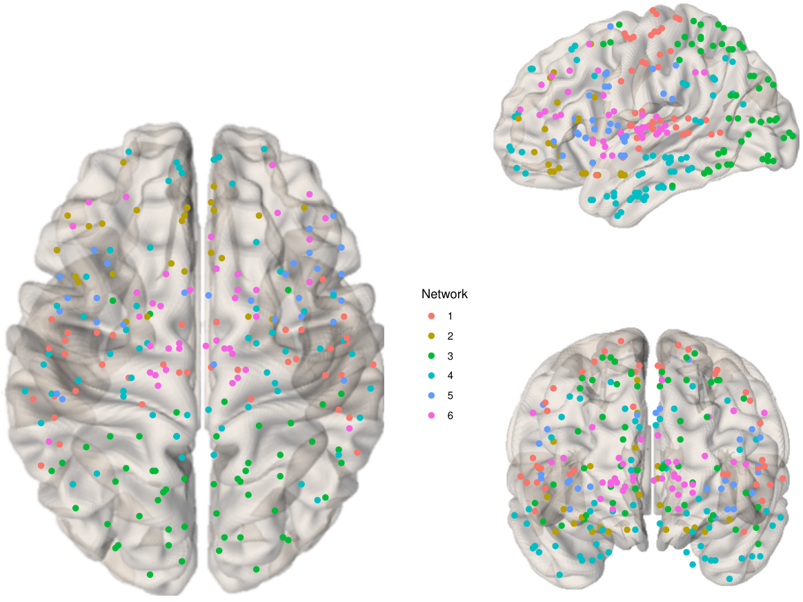
Refer to caption
Figure 8: Clustering result of brain regions by MOP-UP and k-means (k=6k=6)

Appendix C Proof of Theorem 1

We first provide the following lemma:

Lemma 1.

Given a positive definite (semi-positive definite and non-singular) matrix

Σ=[ΣxΣx​zΣx​z⊤Σz]\Sigma=\left[\begin{array}[]{cc}\Sigma_{x}&\Sigma_{xz}\\ \Sigma_{xz}^{\top}&\Sigma_{z}\\ \end{array}\right]

and a random vector xx with 𝔼​x=0\mathbb{E}x=0 and var⁡(x)=Σx{\rm var}(x)=\Sigma_{x}, there exists a random vector zz s.t. 𝔼​z=0\mathbb{E}z=0 and the variance matrix of the joint distribution of (x,z)(x,z) is Σ\Sigma.

Proof.

Notice

[I−Σx−1​Σx​z0I]⊤​[ΣxΣx​zΣx​z⊤Σz]​[I−Σx−1​Σx​z0I]=[Σx00Σz−Σx​z⊤​Σx−1​Σx​z].\left[\begin{array}[]{cc}I&-\Sigma_{x}^{-1}\Sigma_{xz}\\ 0&I\\ \end{array}\right]^{\top}\left[\begin{array}[]{cc}\Sigma_{x}&\Sigma_{xz}\\ \Sigma_{xz}^{\top}&\Sigma_{z}\\ \end{array}\right]\left[\begin{array}[]{cc}I&-\Sigma_{x}^{-1}\Sigma_{xz}\\ 0&I\\ \end{array}\right]=\left[\begin{array}[]{cc}\Sigma_{x}&0\\ 0&\Sigma_{z}-\Sigma_{xz}^{\top}\Sigma_{x}^{-1}\Sigma_{xz}\\ \end{array}\right].

So, Σx\Sigma_{x} and Σz−Σx​z⊤​Σx−1​Σx​z\Sigma_{z}-\Sigma_{xz}^{\top}\Sigma_{x}^{-1}\Sigma_{xz} are positive definite.

There exist z0∼N⁡(0,I)z_{0}\sim N(0,I) such that z0⟂xz_{0}\perp x. Let z=A​z0+B​xz=Az_{0}+Bx. Then 𝔼​z=0\mathbb{E}z=0 and cov⁡(x,z)=Σx​B⊤=Σx​z\operatorname{cov}(x,z)=\Sigma_{x}B^{\top}=\Sigma_{xz} if B=(Σx−1​Σx​y)⊤B=(\Sigma_{x}^{-1}\Sigma_{xy})^{\top}.

Moreover, we have 𝔼​z​z⊤=A​A⊤+B​Σx​B⊤=Σz⇒A​A⊤=Σz−B​Σx​B⊤=Σz−Σx​z⊤​Σx−1​Σx​z\mathbb{E}zz^{\top}=AA^{\top}+B\Sigma_{x}B^{\top}=\Sigma_{z}\Rightarrow AA^{\top}=\Sigma_{z}-B\Sigma_{x}B^{\top}=\Sigma_{z}-\Sigma_{xz}^{\top}\Sigma_{x}^{-1}\Sigma_{xz}. The existence of such AA is guaranteed, since Σz−Σx​z⊤​Σx−1​Σx​z\Sigma_{z}-\Sigma_{xz}^{\top}\Sigma_{x}^{-1}\Sigma_{xz} is positive definite. ∎

Now let’s go back to the proof of Theorem 1.

Proof.

Without loss of generality, assume 𝔼​X=0\mathbb{E}X=0 and σ=1\sigma=1. For tensors 𝐀{\mathbf{A}} and 𝐁{\mathbf{B}}, 𝐀⊗𝐁{\mathbf{A}}\otimes{\mathbf{B}} refers to their tensor product in this section.

Assume the decomposition equation

X=U​A+B​V⊤+ZX=UA+BV^{\top}+Z

holds. Hence, the covariance tensor

𝚺=\displaystyle\boldsymbol{\Sigma}= 𝔼⁡(X⊗X)\displaystyle\mathbb{E}(X\otimes X)
=\displaystyle= 𝔼⁡(U​A+B​V⊤+Z)⊗(U​A+B​V⊤+Z)\displaystyle\mathbb{E}\left(UA+BV^{\top}+Z\right)\otimes\left(UA+BV^{\top}+Z\right)
=\displaystyle= 𝔼⁡(U​A+B​V⊤)⊗(U​A+B​V⊤)+𝐈(p1×p2)2.\displaystyle\mathbb{E}\left(UA+BV^{\top}\right)\otimes\left(UA+BV^{\top}\right)+{\mathbf{I}}_{(p_{1}\times p_{2})_{2}}.

Denote 𝚺0=𝔼⁡(U​A+B​V⊤)⊗(U​A+B​V⊤)\boldsymbol{\Sigma}_{0}=\mathbb{E}\left(UA+BV^{\top}\right)\otimes\left(UA+BV^{\top}\right). Thus,

𝚺0×1U⟂⊤×2V⟂⊤\displaystyle\boldsymbol{\Sigma}_{0}\times_{1}U_{\perp}^{\top}\times_{2}V_{\perp}^{\top}
=\displaystyle= 𝔼((UA)⊗(BV⊤)+(UA)⊗(UA)+(BV⊤)⊗(UA)+(BV⊤)⊗(BV⊤))×1U⟂⊤×2V⟂⊤\displaystyle\mathbb{E}\left((UA)\otimes(BV^{\top})+(UA)\otimes(UA)+(BV^{\top})\otimes(UA)+(BV^{\top})\otimes(BV^{\top})\right)\times_{1}U_{\perp}^{\top}\times_{2}V_{\perp}^{\top}
=\displaystyle= 0,\displaystyle 0,

which proves the sufficiency.

To prove the necessity, assume XX has spiked covariance. Define

A=U⊤​(X−Z),B=PU⟂​(X−Z)​V,A=U^{\top}(X-Z),\qquad B=P_{U_{\perp}}(X-Z)V,

where ZZ is some random matrix with 𝔼​Z=0,𝔼⁡(Z⊗Z)=𝔼⁡(X⊗Z)=𝐈(p1×p2)2\mathbb{E}Z=0,\mathbb{E}(Z\otimes Z)=\mathbb{E}(X\otimes Z)={\mathbf{I}}_{(p_{1}\times p_{2})_{2}}. So 𝔼⁡(A⊗Z)=0\mathbb{E}(A\otimes Z)=0 and 𝔼⁡(B⊗Z)=0\mathbb{E}(B\otimes Z)=0. Here, to see the existence of such ZZ, we can vectorize XX as a random vector. Then, the existence of zz is guaranteed by lemma 1.

Now denote Y=X−Z{Y}={X}-{Z}. Notice ℝp1=span⁡(U)+span⁡(U⟂)\mathbb{R}^{p_{1}}=\operatorname{span}(U)+\operatorname{span}(U_{\perp}) implies that for any u∈ℝp1u\in\mathbb{R}^{p_{1}} we have decomposition u=u1+u2u=u_{1}+u_{2} with u1∈span⁡(U),u2∈span⁡(U⟂)u_{1}\in\operatorname{span}(U),u_{2}\in\operatorname{span}(U_{\perp}) and similar results hold for the case replacing UU by VV. Thus,

u⊤​(Y−U​A−B​V⊤)​v\displaystyle u^{\top}\left(Y-UA-BV^{\top}\right)v
=\displaystyle= u1⊤​(Y−U​A−B​V⊤)​v+u2⊤​(Y−U​A−B​V⊤)​v\displaystyle u_{1}^{\top}\left(Y-UA-BV^{\top}\right)v+u_{2}^{\top}\left(Y-UA-BV^{\top}\right)v
=\displaystyle= u1⊤​(Y−PU​Y−PU⟂​Y​PV)​v+u2⊤​(Y−PU​Y−PU⟂​Y​PV)​v\displaystyle u_{1}^{\top}\left(Y-P_{U}Y-P_{U_{\perp}}YP_{V}\right)v+u_{2}^{\top}\left(Y-P_{U}Y-P_{U_{\perp}}YP_{V}\right)v
=\displaystyle= u2⊤​(Y−PU​Y−PU⟂​Y​PV)​(v1+v2)\displaystyle u_{2}^{\top}\left(Y-P_{U}Y-P_{U_{\perp}}YP_{V}\right)(v_{1}+v_{2})
=\displaystyle= u2⊤​(Y−PU​Y−PU⟂​Y​PV)​v2\displaystyle u_{2}^{\top}\left(Y-P_{U}Y-P_{U_{\perp}}YP_{V}\right)v_{2}
=\displaystyle= u2⊤​Y​v2\displaystyle u_{2}^{\top}Yv_{2}

Notice 𝚺0×1U⟂×2V⟂=0\boldsymbol{\Sigma}_{0}\times_{1}U_{\perp}\times_{2}V_{\perp}=0 implies that for any u2∈span⁡(U⟂),v2∈span⁡(V⟂),u3∈ℝp1u_{2}\in\operatorname{span}(U_{\perp}),v_{2}\in\operatorname{span}(V_{\perp}),u_{3}\in\mathbb{R}^{p_{1}} and v3∈ℝp2,v_{3}\in\mathbb{R}^{p_{2}}, we have 𝚺0​(u2,v2,u3,v3)=0\boldsymbol{\Sigma}_{0}(u_{2},v_{2},u_{3},v_{3})=0. Thus, for any vectors u,v,u′,v′u,v,u^{\prime},v^{\prime} with suitable dimensions,

(𝔼⁡(Y−U​A−B​V⊤)⊗(Y−U​A−B​V⊤))​(u,v,u′,v′)\displaystyle\left(\mathbb{E}\left(Y-UA-BV^{\top}\right)\otimes\left(Y-UA-BV^{\top}\right)\right)(u,v,u^{\prime},v^{\prime})
=\displaystyle= 𝔼​u⊤​(Y−U​A−B​V⊤)​v​u′⊤​(Y−U​A−B​V⊤)​v′\displaystyle\mathbb{E}u^{\top}\left(Y-UA-BV^{\top}\right)v{u^{\prime}}^{\top}\left(Y-UA-BV^{\top}\right)v^{\prime}
=\displaystyle= 𝔼​u2⊤​Y​v2​u2′⊤​Y​v2′\displaystyle\mathbb{E}u_{2}^{\top}Yv_{2}{u_{2}^{\prime}}^{\top}Yv^{\prime}_{2}
=\displaystyle= 𝚺0​(u2,v2,u2′,v2′)\displaystyle\boldsymbol{\Sigma}_{0}(u_{2},v_{2},u_{2}^{\prime},v_{2}^{\prime})
=\displaystyle= 0,\displaystyle 0,

i.e., the covariance tensor is 0, and hence, the decomposition equation holds a.s. Thus, the theorem is proved. ∎

Appendix D Proof of Theorem 2

Proof.

Assume that for some U′,V′U^{\prime},V^{\prime} we have PU⟂′​Y​PV⟂′=0.P_{U^{\prime}_{\perp}}YP_{V^{\prime}_{\perp}}=0. Notice that ‖sin⁡Θ⁡(U,U′)‖=0\|\sin\Theta(U,U^{\prime})\|=0 is equivalent to PU⟂′​U=0P_{U^{\prime}_{\perp}}U=0. Now assume PU⟂′​U≠0P_{U^{\prime}_{\perp}}U\neq 0. We have

0=\displaystyle 0= PU⟂′​Y​PV⟂′\displaystyle P_{U^{\prime}_{\perp}}YP_{V^{\prime}_{\perp}}
=\displaystyle= PU⟂′​(U​A+B​V⊤)​PV⟂′\displaystyle P_{U^{\prime}_{\perp}}(UA+BV^{\top})P_{V^{\prime}_{\perp}}
=\displaystyle= PU⟂′​U​A​PV⟂′+PU⟂′​B​V⊤​PV⟂′.\displaystyle P_{U^{\prime}_{\perp}}UAP_{V^{\prime}_{\perp}}+P_{U^{\prime}_{\perp}}BV^{\top}P_{V^{\prime}_{\perp}}.

Intuitively, to make the last line 0, we need its two terms to cancel out with each other. However, by the condition in the theorem, the probability for PU⟂′​U​A​PV⟂′P_{U^{\prime}_{\perp}}UAP_{V^{\prime}_{\perp}} to cancel out with PU⟂′​B​V⊤​PV⟂′P_{U^{\prime}_{\perp}}BV^{\top}P_{V^{\prime}_{\perp}} for any given BB is strictly less than 1.

To make the statement rigorous, notice that it follows span⁡(U​A​PV⟂′+B​V⊤​PV⟂′)⊆ker⁡(PU⟂′)\operatorname{span}\left(UAP_{V^{\prime}_{\perp}}+BV^{\top}P_{V^{\prime}_{\perp}}\right)\subseteq\ker(P_{U^{\prime}_{\perp}}), which implies for any vv such that PV⟂′​v≠0P_{V^{\prime}_{\perp}}v\neq 0, we have

U​A​PV⟂′​v+B​V⊤​PV⟂′​v∈ker⁡(PU⟂′),UAP_{V^{\prime}_{\perp}}v+BV^{\top}P_{V^{\prime}_{\perp}}v\in\ker(P_{U^{\prime}_{\perp}}),

and hence

U​A​PV⟂′​v∈𝒜,UAP_{V^{\prime}_{\perp}}v\in\mathcal{A},

where 𝒜\mathcal{A} represents the affine space {u−B​V⊤​PV⟂′​v:∀u∈ker⁡(PU⟂′)}\{u-BV^{\top}P_{V^{\prime}_{\perp}}v:\forall u\in\ker(P_{U^{\prime}_{\perp}})\}.

For given BB, if B​V⊤​PV⟂′​v=0BV^{\top}P_{V^{\prime}_{\perp}}v=0, we have 𝒜=ker⁡(PU⟂′)=span⁡(U′)≠span⁡(U)\mathcal{A}=\ker(P_{U^{\prime}_{\perp}})=\operatorname{span}(U^{\prime})\neq\operatorname{span}(U), and thus span⁡(U)⊈𝒜\operatorname{span}(U)\not\subseteq\mathcal{A}.

If B​V⊤​PV⟂′​v≠0BV^{\top}P_{V^{\prime}_{\perp}}v\neq 0, then 𝒜\mathcal{A} is a shifted r1r_{1} dimensional space. If the shift direction is in the subspace, i.e., B​V⊤​PV⟂′​v∈ker⁡(PU⟂′)BV^{\top}P_{V^{\prime}_{\perp}}v\in\ker(P_{U^{\prime}_{\perp}}), then 𝒜=ker⁡(PU⟂′)\mathcal{A}=\ker(P_{U^{\prime}_{\perp}}), and hence span⁡(U)⊈𝒜\operatorname{span}(U)\not\subseteq\mathcal{A}. If the shift direction is not in the subspace, i.e., B​V⊤​PV⟂′​v∉ker⁡(PU⟂′)BV^{\top}P_{V^{\prime}_{\perp}}v\notin\ker(P_{U^{\prime}_{\perp}}), then for any u∈span⁡(U)u\in\operatorname{span}(U) with small enough ‖u‖\|u\|, we have u∉𝒜u\notin\mathcal{A}. Thus, span⁡(U)⊈𝒜\operatorname{span}(U)\not\subseteq\mathcal{A}.

By the discussion above, we always have span⁡(U)⊈𝒜\operatorname{span}(U)\not\subseteq\mathcal{A}. Hence by the condition in the theorem, we have ℙ⁡(U​A​PV⟂′​v∈𝒜|B)<1\mathbb{P}(UAP_{V^{\prime}_{\perp}}v\in\mathcal{A}|B)<1, which concludes that

ℙ⁡(PU⟂′​Y​PV⟂′=0)≤𝔼⁡(ℙ⁡(U​A​PV⟂′​v∈𝒜|B))<1.\mathbb{P}\left(P_{U^{\prime}_{\perp}}YP_{V^{\prime}_{\perp}}=0\right)\leq\mathbb{E}\left(\mathbb{P}(UAP_{V^{\prime}_{\perp}}v\in\mathcal{A}|B)\right)<1.

Thus, by Theorem 1, if the covariance tensor 𝚺\boldsymbol{\Sigma} of YY satisfies 𝚺×1U′⟂×2V′⟂=0\boldsymbol{\Sigma}\times_{1}U^{\prime}_{\perp}\times_{2}V^{\prime}_{\perp}=0, then there exist some A′,B′A^{\prime},B^{\prime} such that Y=U′​A′+B′​V′⊤Y=U^{\prime}A^{\prime}+B^{\prime}{V^{\prime}}^{\top}, and hence there must be ℙ⁡(PU⟂′​Y​PV⟂′=0)=1\mathbb{P}\left(P_{U^{\prime}_{\perp}}YP_{V^{\prime}_{\perp}}=0\right)=1. Contradict. Thus, 𝚺×1U′⟂×2V′⟂≠0\boldsymbol{\Sigma}\times_{1}U^{\prime}_{\perp}\times_{2}V^{\prime}_{\perp}\neq 0. ∎

Appendix E Proof of Theorem 3

We first introduce the following technical lemmas.

Lemma 2.

Let AA and BB be two mm-by-nn matrices. If ker⁡(B)+ker⁡(A)=ℝn\ker(B)+\ker(A)=\mathbb{R}^{n}, then we have span⁡(A)⊆span⁡(A+B)\operatorname{span}(A)\subseteq\operatorname{span}(A+B). If AA and BB further satisfy span⁡(A)∩span⁡(B)={0}\operatorname{span}(A)\cap\operatorname{span}(B)=\{0\}, then span⁡(A)⊆span⁡(A+B)\operatorname{span}(A)\subseteq\operatorname{span}(A+B) if and only if ker⁡(B)+ker⁡(A)=ℝn\ker(B)+\ker(A)=\mathbb{R}^{n}.

Proof.

For any u∈ℝnu\in\mathbb{R}^{n}, we have

u∈ker⁡(B)+ker⁡(A)\displaystyle u\in\ker(B)+\ker(A)
⇔\displaystyle\Leftrightarrow ∃a0∈ker⁡(A),b0∈ker⁡(B):u=a0+b0\displaystyle\exists a_{0}\in\ker(A),b_{0}\in\ker(B):u=a_{0}+b_{0}
⇔\displaystyle\Leftrightarrow −a0∈ker⁡(A)​ and ​u−a0∈ker⁡(B)\displaystyle-a_{0}\in\ker(A)\text{ and }u-a_{0}\in\ker(B)
⇒\displaystyle\Rightarrow A​u=(A+B)​(u−a0)\displaystyle Au=(A+B)(u-a_{0})
⇒\displaystyle\Rightarrow A​u∈span⁡(A+B).\displaystyle Au\in\operatorname{span}(A+B).

Thus, as uu can be arbitrary, it follows that span⁡(A)⊆span⁡(A+B)\operatorname{span}(A)\subseteq\operatorname{span}(A+B).

If we further have span⁡A∩span⁡B={0}\operatorname{span}A\cap\operatorname{span}B=\{0\}, then for any u∈ℝnu\in\mathbb{R}^{n}, it follows that

span⁡(A)⊆span⁡(A+B)\displaystyle\operatorname{span}(A)\subseteq\operatorname{span}(A+B)
⇒\displaystyle\Rightarrow ∃v:(A+B)​v=A​u\displaystyle\exists v:(A+B)v=Au
⇔\displaystyle\Leftrightarrow A⁡(u−v)=B​v\displaystyle A(u-v)=Bv
⇒\displaystyle\Rightarrow u−v∈ker⁡(A),v∈ker⁡(B)\displaystyle u-v\in\ker(A),v\in\ker(B)
⇔\displaystyle\Leftrightarrow u∈ker⁡(B)+ker⁡(A).\displaystyle u\in\ker(B)+\ker(A).

∎

Lemma 3.

If AA is a pp-by-rAr_{A} random matrix with density in ℝp​rA\mathbb{R}^{pr_{A}} and BB is a pp-by-rBr_{B} deterministic matrix, rA,rB≤pr_{A},r_{B}\leq p, then we have

ℙ⁡(dim(span⁡(A)∩span⁡(B))=max⁡{0,rA+rB−p})=1.\mathbb{P}\left(\dim(\operatorname{span}(A)\cap\operatorname{span}(B))=\max\{0,r_{A}+r_{B}-p\}\right)=1.
Proof.

Denote A=[a1,⋯,arA]A=[a_{1},\cdots,a_{r_{A}}] and B=[b1,⋯,brB]B=[b_{1},\cdots,b_{r_{B}}]. Let’s prove this by induction. Consider the case that rA=1r_{A}=1. The case when p=1p=1 is trivial. If p≥2p\geq 2, we have

ℙ⁡(dim(span⁡(A)∩span⁡(B))=1)=ℙ⁡(a1∈span⁡(B)⊊ℝp)=0.\mathbb{P}(\dim(\operatorname{span}(A)\cap\operatorname{span}(B))=1)=\mathbb{P}(a_{1}\in\operatorname{span}(B)\subsetneq\mathbb{R}^{p})=0.

Thus,

ℙ⁡(dim(span⁡(A)∩span⁡(B))=0=max⁡{0,rA+rB−p})=1.\mathbb{P}(\dim(\operatorname{span}(A)\cap\operatorname{span}(B))=0=\max\{0,r_{A}+r_{B}-p\})=1.

Before going to the induction step, notice the following fact: as the joint density of a1,⋯,arAa_{1},\cdots,a_{r_{A}} exists, we have the conditional density of arA|A−rA:=arA|a1,⋯,arA−1a_{r_{A}}|A_{-r_{A}}:=a_{r_{A}}|a_{1},\cdots,a_{r_{A}-1}, i.e., the conditional distribution arA|A−rAa_{r_{A}}|A_{-r_{A}} is almost surely absolutely continuous with respect to Lebesgue measure.

Now we assume the lemma holds for rA=mA−1r_{A}=m_{A}-1 and rB=mBr_{B}=m_{B}. Consider the case rA=mA≥2r_{A}=m_{A}\geq 2 and rB=mBr_{B}=m_{B}.

If p≥rA+rBp\geq r_{A}+r_{B}, then denote A−rA=[a1,⋯,arA−1]A_{-r_{A}}=[a_{1},\cdots,a_{r_{A}-1}] and by induction, we have

ℙ⁡(dim(span⁡(A−rA)∩span⁡(B))=0)=1.\mathbb{P}(\dim(\operatorname{span}(A_{-r_{A}})\cap\operatorname{span}(B))=0)=1.

And by p>rB+rA−1,p>r_{B}+r_{A}-1, we have

span⁡(B)+span⁡(A−rA)⊊ℝp.\operatorname{span}(B)+\operatorname{span}(A_{-r_{A}})\subsetneq\mathbb{R}^{p}.

Thus, as the Lebesgue measure of any nontrivial subspace is 0 and arA|A−rAa_{r_{A}}|A_{-r_{A}} is absolutely continuous with respect to the Lebesgue measure almost surely, we know

ℙ⁡(arA∈span⁡(B)+span⁡(A−rA)|A−rA)=0,\mathbb{P}(a_{r_{A}}\in\operatorname{span}(B)+\operatorname{span}(A_{-r_{A}})|A_{-r_{A}})=0,

and

ℙ⁡(arA∈span⁡(A−rA)|A−rA)=0.\mathbb{P}(a_{r_{A}}\in\operatorname{span}(A_{-r_{A}})|A_{-r_{A}})=0.

Further notice if for some uu such that 0≠u∈span⁡(A)+span⁡(B)0\neq u\in\operatorname{span}(A)+\operatorname{span}(B) but u∉span⁡(A−rA)+span⁡(B)u\notin\operatorname{span}(A_{-r_{A}})+\operatorname{span}(B), then u=a+bu=a+b for some nonzero a∈span⁡(A)a\in\operatorname{span}(A), a∉span⁡(A−rA)a\notin\operatorname{span}(A_{-r_{A}}) and b∈span⁡(B)b\in\operatorname{span}(B). Then, we have a=a0+c⋅arAa=a_{0}+c\cdot a_{r_{A}} with a0∈span⁡(A−rA)a_{0}\in\operatorname{span}(A_{-r_{A}}) and some nonzero c ∈ℝ\in\mathbb{R}. Thus, c⋅arA=u−a0−b∈span⁡(B)+span⁡(A−rA)c\cdot a_{r_{A}}=u-a_{0}-b\in\operatorname{span}(B)+\operatorname{span}(A_{-r_{A}}), which yields that

ℙ⁡(dim(span⁡(A)∩span⁡(B))≥1+dim(span⁡(A−rA)∩span⁡(B)))\displaystyle\mathbb{P}(\dim(\operatorname{span}(A)\cap\operatorname{span}(B))\geq 1+\dim(\operatorname{span}(A_{-r_{A}})\cap\operatorname{span}(B)))
=\displaystyle= ℙ⁡(span⁡(A)∩span⁡(B)⊋span⁡(A−rA)∩span⁡(B))\displaystyle\mathbb{P}(\operatorname{span}(A)\cap\operatorname{span}(B)\supsetneq\operatorname{span}(A_{-r_{A}})\cap\operatorname{span}(B))
≤\displaystyle\leq 𝔼⁡(ℙ⁡(arA∈span⁡(B)+span⁡(A−rA)|A−rA))\displaystyle\mathbb{E}(\mathbb{P}(a_{r_{A}}\in\operatorname{span}(B)+\operatorname{span}(A_{-r_{A}})|A_{-r_{A}}))
=\displaystyle= 0.\displaystyle 0.

Hence, ℙ⁡(dim(span⁡(A)∩span⁡(B))=0)=1\mathbb{P}(\dim(\operatorname{span}(A)\cap\operatorname{span}(B))=0)=1.

If p≤rA+rB−1p\leq r_{A}+r_{B}-1, then we have ℙ⁡(dim(span⁡(A−rA)∩span⁡(B))=0)=1\mathbb{P}(\dim(\operatorname{span}(A_{-r_{A}})\cap\operatorname{span}(B))=0)=1. But this time we have ℙ⁡(dim(span⁡(A−rA)+span⁡(B))=ℝp)=1\mathbb{P}(\dim(\operatorname{span}(A_{-r_{A}})+\operatorname{span}(B))=\mathbb{R}^{p})=1 and thus ℙ⁡(arA∈span⁡(A−rA)+span⁡(B)|A−rA)=1\mathbb{P}(a_{r_{A}}\in\operatorname{span}(A_{-r_{A}})+\operatorname{span}(B)|A_{-r_{A}})=1. We can similarly prove that

ℙ⁡(span⁡(A)∩span⁡(B)=span⁡(A−rA)∩span⁡(B))\displaystyle\mathbb{P}(\operatorname{span}(A)\cap\operatorname{span}(B)=\operatorname{span}(A_{-r_{A}})\cap\operatorname{span}(B))
≤\displaystyle\leq 𝔼⁡(ℙ⁡(arA∉span⁡(B)+span⁡(A−rA)|A−rA))\displaystyle\mathbb{E}(\mathbb{P}(a_{r_{A}}\notin\operatorname{span}(B)+\operatorname{span}(A_{-r_{A}})|A_{-r_{A}}))
=\displaystyle= 0,\displaystyle 0,

which indicates that ℙ⁡(dim(span⁡(A)∩span⁡(B))=dim(span⁡(A−rA)∩span⁡(B))+1=rA+rB−p)=1\mathbb{P}(\dim(\operatorname{span}(A)\cap\operatorname{span}(B))=\dim(\operatorname{span}(A_{-r_{A}})\cap\operatorname{span}(B))+1=r_{A}+r_{B}-p)=1. These complete the induction step and the lemma holds. ∎

Now we are ready to prove Theorem 3.

Proof.

Let’s first prove span⁡(U)⊆⋂i=1nspan⁡(Xi)\operatorname{span}(U)\subseteq\bigcap_{i=1}^{n}\operatorname{span}(X_{i}).

By comparing the dimension of both sides, we have the following facts: 1. ker⁡(V⊤)=ker⁡(B​V⊤)\ker(V^{\top})=\ker(BV^{\top}); 2. span⁡(U)=span⁡(U​A)\operatorname{span}(U)=\operatorname{span}(UA); and 3. ker⁡(A)=ker⁡(U​A)\ker(A)=\ker(UA).

Notice Lemma 3 applies to A⊤A^{\top} and VV, which yields span⁡(A⊤)∩span⁡(V)={0}\operatorname{span}(A^{\top})\cap\operatorname{span}(V)=\{0\} almost surely. Thus,

span⁡(A⊤)∩span⁡(B⊤)={0}\displaystyle\operatorname{span}(A^{\top})\cap\operatorname{span}(B^{\top})=\{0\}
⇒\displaystyle\Rightarrow ℝp2={0}⟂=(span⁡(A⊤)∩span⁡(V))⟂=span⁡(A⊤)⟂+span⁡(V)⟂\displaystyle\mathbb{R}^{p_{2}}=\{0\}^{\perp}=(\operatorname{span}(A^{\top})\cap\operatorname{span}(V))^{\perp}=\operatorname{span}(A^{\top})^{\perp}+\operatorname{span}(V)^{\perp}
=ker⁡(A)+ker⁡(V⊤)=ker⁡(U​A)+ker⁡(B​V⊤)\displaystyle\quad=\ker(A)+\ker(V^{\top})=\ker(UA)+\ker(BV^{\top})
⇒(Lemma 2)\displaystyle\overset{\text{(Lemma \ref{lemma_span_sum})}}{\Rightarrow} span⁡(U)=span⁡(U​A)⊆span⁡(U​A+B​V⊤).\displaystyle\operatorname{span}(U)=\operatorname{span}(UA)\subseteq\operatorname{span}(UA+BV^{\top}).

It proves span⁡(U)⊆⋂i=1nspan⁡(Xi)\operatorname{span}(U)\subseteq\bigcap_{i=1}^{n}\operatorname{span}(X_{i}) almost surely.

Before prove the other direction, let’s firstly prove ⋂i=1nspan⁡(U⟂⊤​Bi)={0}\bigcap_{i=1}^{n}\operatorname{span}(U_{\perp}^{\top}B_{i})=\{0\}. Notice the density of U⟂⊤​BU_{\perp}^{\top}B exists, and {Bi}\{B_{i}\} are i.i.d. copies of BB. So, by Lemma 3, we have dim(span⁡(U⟂⊤​B1)∩span⁡(U⟂⊤​B2))=max⁡{0,2​r2−(p1−r1)}\dim(\operatorname{span}(U_{\perp}^{\top}B_{1})\cap\operatorname{span}(U_{\perp}^{\top}B_{2}))=\max\{0,2r_{2}-(p_{1}-r_{1})\} almost surely. If 2​r2−(p1−r1)≤02r_{2}-(p_{1}-r_{1})\leq 0, then it is done. If 2​r2−(p1−r1)>02r_{2}-(p_{1}-r_{1})>0, then we consider dim((span⁡(U⟂⊤​B1)∩span⁡(U⟂⊤​B2))∩span⁡(U⟂⊤​B3))\dim((\operatorname{span}(U_{\perp}^{\top}B_{1})\cap\operatorname{span}(U_{\perp}^{\top}B_{2}))\cap\operatorname{span}(U_{\perp}^{\top}B_{3})). Notice given B1B_{1} and B2B_{2}, (span⁡(U⟂⊤​B1)∩span⁡(U⟂⊤​B2))=span⁡(D)(\operatorname{span}(U_{\perp}^{\top}B_{1})\cap\operatorname{span}(U_{\perp}^{\top}B_{2}))=\operatorname{span}(D) for some (p1−r1)(p_{1}-r_{1})-by-(2​r2−(p1−r1))(2r_{2}-(p_{1}-r_{1})) matrix DD. Then apply Lemma 3 to U⟂⊤​B3U_{\perp}^{\top}B_{3} and DD, which yields dim(span⁡(U⟂⊤​B1)∩span⁡(U⟂⊤​B2)∩span⁡(U⟂⊤​B3))=max⁡{0,3​r2−2​(p1−r1)}\dim(\operatorname{span}(U_{\perp}^{\top}B_{1})\cap\operatorname{span}(U_{\perp}^{\top}B_{2})\cap\operatorname{span}(U_{\perp}^{\top}B_{3}))=\max\{0,3r_{2}-2(p_{1}-r_{1})\}. We repeat this procedure until k​r2−(k−1)​(p1−r1)≤0kr_{2}-(k-1)(p_{1}-r_{1})\leq 0 for some kk. n​r2−(n−1)​(p1−r1)≤0nr_{2}-(n-1)(p_{1}-r_{1})\leq 0 guarantees that it will stop before (or at) k=nk=n, which will yield ⋂i=1nspan⁡(U⟂⊤​Bi)=0\bigcap_{i=1}^{n}\operatorname{span}(U_{\perp}^{\top}B_{i})={0} almost surely.

Now let’s go back to prove span⁡(U)⊇⋂i=1nspan⁡(Xi)\operatorname{span}(U)\supseteq\bigcap_{i=1}^{n}\operatorname{span}(X_{i}). Notice for some vectors vi∈ℝp2v_{i}\in\mathbb{R}^{p_{2}}, if Xi​vi=Xj​vjX_{i}v_{i}=X_{j}v_{j} for all i,j∈{1,⋯n},i,j\in\{1,\cdots n\}, then it follows

U⟂⊤​X1​v1=⋯=U⟂⊤​Xn​vn\displaystyle U_{\perp}^{\top}X_{1}v_{1}=\cdots=U_{\perp}^{\top}X_{n}v_{n}
⇒\displaystyle\Rightarrow U⟂⊤​B1​V⊤​v1=⋯=U⟂⊤​Bn​V⊤​vn.\displaystyle U_{\perp}^{\top}B_{1}V^{\top}v_{1}=\cdots=U_{\perp}^{\top}B_{n}V^{\top}v_{n}.

Recall that we have proved ⋂i=1nspan⁡(U⟂⊤​Bi)={0}\bigcap_{i=1}^{n}\operatorname{span}(U_{\perp}^{\top}B_{i})=\{0\} almost surely, which implies U⟂⊤​Bi​V⊤​vi=0U_{\perp}^{\top}B_{i}V^{\top}v_{i}=0 and hence Xi​vi=(PU+PU⟂)​Xi​vi=PU​Xi​vi∈span⁡(U)X_{i}v_{i}=(P_{U}+P_{U_{\perp}})X_{i}v_{i}=P_{U}X_{i}v_{i}\in\operatorname{span}(U). Thus, span⁡(U)⊇⋂i=1nspan⁡(Xi)\operatorname{span}(U)\supseteq\bigcap_{i=1}^{n}\operatorname{span}(X_{i}) almost surely, which finishes the proof. ∎

Appendix F Proof of Theorem 4

Proof.

Denote r=r1+r2r=r_{1}+r_{2}, Qi=SVDr​(Xi)Q_{i}={\rm SVD}_{r}\left(X_{i}\right), Yi=U​Ai+Bi​V⊤Y_{i}=UA_{i}+B_{i}V^{\top}, Q~i=SVDr​(Yi)\tilde{Q}_{i}={\rm SVD}_{r}\left(Y_{i}\right), U~=Eigenr1​(1n​∑i=1nQ~i​Q~i⊤)\tilde{U}={\rm Eigen}_{r_{1}}\left(\frac{1}{n}\sum_{i=1}^{n}\tilde{Q}_{i}{\tilde{Q}_{i}}^{\top}\right) and P~i=Q~i​Q~i⊤\tilde{P}_{i}=\tilde{Q}_{i}{\tilde{Q}_{i}}^{\top}. Then by Theorem 3, we have P~i=PU+P^i\tilde{P}_{i}=P_{U}+\hat{P}_{i}, where P^i\hat{P}_{i} is some projection matrix such that span⁡(P^i)⊆span⁡(U⟂)\operatorname{span}(\hat{P}_{i})\subseteq\operatorname{span}(U_{\perp}) almost surely. Thus, λr1​(1n​∑i=1nP~i)=1\lambda_{r_{1}}(\frac{1}{n}\sum_{i=1}^{n}\tilde{P}_{i})=1 almost surely.

Then we have

‖sin⁡Θ⁡(U^,U)‖≤‖sin⁡Θ⁡(U^,U~)‖+|sin⁡Θ⁡(U~,U)|=‖sin⁡Θ⁡(U^,U~)‖,\|\sin\Theta(\hat{U},U)\|\leq\|\sin\Theta(\hat{U},\tilde{U})\|+\|\sin\Theta(\tilde{U},U)\|=\|\sin\Theta(\hat{U},\tilde{U})\|,

where ‖sin⁡Θ⁡(U~,U)‖=0\|\sin\Theta(\tilde{U},U)\|=0 is yielded by Corollary 1. To bound ‖sin⁡Θ⁡(U^,U~)‖\|\sin\Theta(\hat{U},\tilde{U})\|, we can use the matrix perturbation theory. In the setup of X^=X+Z\hat{X}=X+Z, we can let X=1n​∑i=1nP~iX=\frac{1}{n}\sum_{i=1}^{n}\tilde{P}_{i} and X^=1n​∑i=1nQi​Qi⊤\hat{X}=\frac{1}{n}\sum_{i=1}^{n}Q_{i}{Q_{i}}^{\top}. Davis-Khan Theorem (e.g. Corollary 2.8 in Chen et al., 2021) yields

‖sin⁡Θ⁡(U^,U~)‖≤2​‖1n​∑i=1n(P~i−Qi​Qi⊤)‖λr1​(1n​∑i=1nP~i)−λr1+1​(1n​∑i=1nP~i).\|\sin\Theta(\hat{U},\tilde{U})\|\leq\frac{\sqrt{2}\left\|\frac{1}{n}\sum_{i=1}^{n}(\tilde{P}_{i}-Q_{i}{Q_{i}}^{\top})\right\|}{\lambda_{r_{1}}(\frac{1}{n}\sum_{i=1}^{n}\tilde{P}_{i})-\lambda_{r_{1}+1}(\frac{1}{n}\sum_{i=1}^{n}\tilde{P}_{i})}. (18)

We are going to upper bound the numerator and lower bound the denominator of (18).

F.0.1 Numerator

we can use Matrix Chernoff bound (e.g., Tropp, 2012):

Lemma 4 (Matrix Chernoff).

Consider a finite sequence {𝐗k}\left\{\boldsymbol{X}_{k}\right\} of independent, random, self-adjoint matrices that satisfy

𝑿k≽𝟎 and λmax​(𝑿k)≤R almost surely. \boldsymbol{X}_{k}\succcurlyeq\mathbf{0}\quad\text{ and }\quad\lambda_{\max}\left(\boldsymbol{X}_{k}\right)\leq R\quad\text{ almost surely. }

Compute the minimum and maximum eigenvalues of the sum of expectations,

μmax:=λmax​(∑k𝔼​𝑿k)​. \mu_{\max}:=\lambda_{\max}\left(\sum_{k}\mathbb{E}\boldsymbol{X}_{k}\right)\text{. }

Then

ℙ{λmax(∑k𝑿k)≥(1+δ)μmax}≤d⋅[eδ(1+δ)1+δ]μmax/R for δ≥0.\displaystyle\mathbb{P}\left\{\lambda_{\max}\left(\sum_{k}\boldsymbol{X}_{k}\right)\geq(1+\delta)\mu_{\max}\right\}\leq d\cdot\left[\frac{\mathrm{e}^{\delta}}{(1+\delta)^{1+\delta}}\right]^{\mu_{\max}/R}\quad\text{ for }\delta\geq 0.

Notice here our matrices P~i−Qi​Qi⊤\tilde{P}_{i}-Q_{i}{Q_{i}}^{\top} are not necessarily p.s.d. but they are bounded by ‖Q~i​Q~i⊤−Qi​Qi⊤‖≤1\|\tilde{Q}_{i}\tilde{Q}_{i}^{\top}-Q_{i}{Q_{i}}^{\top}\|\leq 1 (the operator norm of the difference of projectors are bounded by 1). So, we can let Wi=Q~i​Q~i⊤−Qi​Qi⊤+IW_{i}=\tilde{Q}_{i}\tilde{Q}_{i}^{\top}-Q_{i}{Q_{i}}^{\top}+I, then WiW_{i} are p.s.d. and we can apply Matrix Chernoff bound to WiW_{i}, which yields

ℙ{λ1(1n∑kWk)≥(1+δ)​μmaxn}≤p1⋅[eδ(1+δ)1+δ]μmax/2 for ∀δ≥0.\displaystyle\mathbb{P}\left\{\lambda_{1}\left(\frac{1}{n}\sum_{k}W_{k}\right)\geq\frac{(1+\delta)\mu_{\max}}{n}\right\}\leq p_{1}\cdot\left[\frac{\mathrm{e}^{\delta}}{(1+\delta)^{1+\delta}}\right]^{\mu_{\max}/2}\quad\text{ for }\forall\delta\geq 0. (19)

To bound μmax=n​λ1​(𝔼​W1)=n​λ1​(𝔼​P~1−𝔼​Q1​Q1⊤)+n\mu_{\max}=n\lambda_{1}(\mathbb{E}W_{1})=n\lambda_{1}(\mathbb{E}\tilde{P}_{1}-\mathbb{E}Q_{1}{Q_{1}}^{\top})+n, we use self adjoint dilation and Theorem 1 in Xia, 2021, where we let

A^=(0X1X1⊤0),A=(0Y1Y1⊤0),\hat{A}=\left(\begin{array}[]{cc}0&X_{1}\\ X_{1}^{\top}&0\end{array}\right),\quad A=\left(\begin{array}[]{cc}0&Y_{1}\\ Y_{1}^{\top}&0\end{array}\right),

and

X=(0Z1Z1⊤0).X=\left(\begin{array}[]{cc}0&Z_{1}\\ Z_{1}^{\top}&0\end{array}\right).

Denote Θ^​Θ^⊤:=diag⁡(Qi​Qi⊤,Hi​Hi⊤)\hat{\Theta}\hat{\Theta}^{\top}:={\rm diag}(Q_{i}{Q_{i}}^{\top},H_{i}{H_{i}}^{\top}), Θ​Θ⊤:=diag⁡(P~i,H~i​H~i⊤)\Theta\Theta^{\top}:={\rm diag}(\tilde{P}_{i},\tilde{H}_{i}{\tilde{H}_{i}}^{\top}), Hi,H~iH_{i},\tilde{H}_{i} are the first r1+r2r_{1}+r_{2} right singular vectors of U​A+B​V⊤+ZUA+BV^{\top}+Z and U​A+B​V⊤UA+BV^{\top} respectively, the event 𝒜:={4∥Z∥≤cσr(Y)}\mathcal{A}:=\{4\|Z\|\leq c\sigma_{r}(Y)\} for some c<1c<1 and I{𝒜}I_{\{\mathcal{A}\}} is the indicator function of event 𝒜\mathcal{A}. Then it yields that

μmax−n=\displaystyle\mu_{\max}-n= n⁡‖𝔼​Qi​Qi⊤−𝔼​P~i‖\displaystyle n\left\|\mathbb{E}Q_{i}{Q_{i}}^{\top}-\mathbb{E}\tilde{P}_{i}\right\|
≤\displaystyle\leq n⁡‖𝔼⁡(Θ^​Θ^⊤−Θ​Θ⊤)‖\displaystyle n\left\|\mathbb{E}\left(\hat{\Theta}\hat{\Theta}^{\top}-\Theta\Theta^{\top}\right)\right\|
=\displaystyle= n⁡‖𝔼⁡(Θ^​Θ^⊤−Θ​Θ⊤)​diag​(I{𝒜})+𝔼⁡(Θ^​Θ^⊤−Θ​Θ⊤)​diag​(I{𝒜c})‖\displaystyle n\left\|\mathbb{E}\left(\hat{\Theta}\hat{\Theta}^{\top}-\Theta\Theta^{\top}\right){\rm diag}(I_{\{\mathcal{A}\}})+\mathbb{E}\left(\hat{\Theta}\hat{\Theta}^{\top}-\Theta\Theta^{\top}\right){\rm diag}(I_{\{\mathcal{A}^{c}\}})\right\|
≤\displaystyle\leq n⁡‖𝔼⁡(Θ^​Θ^⊤−Θ​Θ⊤)​diag​(I{𝒜})‖+n​𝔼​‖(Θ^​Θ^⊤−Θ​Θ⊤)​diag​(I{𝒜c})‖\displaystyle n\left\|\mathbb{E}\left(\hat{\Theta}\hat{\Theta}^{\top}-\Theta\Theta^{\top}\right){\rm diag}(I_{\{\mathcal{A}\}})\right\|+n\mathbb{E}\left\|\left(\hat{\Theta}\hat{\Theta}^{\top}-\Theta\Theta^{\top}\right){\rm diag}(I_{\{\mathcal{A}^{c}\}})\right\|
≤\displaystyle\leq n⁡‖𝔼⁡(Θ^​Θ^⊤−Θ​Θ⊤)​diag​(I{𝒜})‖+n​ℙ​(𝒜c)\displaystyle n\left\|\mathbb{E}\left(\hat{\Theta}\hat{\Theta}^{\top}-\Theta\Theta^{\top}\right){\rm diag}(I_{\{\mathcal{A}\}})\right\|+n\mathbb{P}(\mathcal{A}^{c})
=\displaystyle= n⁡‖𝔼⁡(Θ^​Θ^⊤−Θ​Θ⊤−𝒮A,1)​diag​(I{𝒜})‖+n​ℙ​(𝒜c)\displaystyle n\left\|\mathbb{E}\left(\hat{\Theta}\hat{\Theta}^{\top}-\Theta\Theta^{\top}-\mathcal{S}_{A,1}\right){\rm diag}(I_{\{\mathcal{A}\}})\right\|+n\mathbb{P}(\mathcal{A}^{c})
≤\displaystyle\leq n​𝔼​‖diag⁡(I{𝒜})​(Θ^​Θ^⊤−Θ​Θ⊤−𝒮A,1)‖+n​ℙ​(𝒜c)\displaystyle n\mathbb{E}\left\|{\rm diag}(I_{\{\mathcal{A}\}})\left(\hat{\Theta}\hat{\Theta}^{\top}-\Theta\Theta^{\top}-\mathcal{S}_{A,1}\right)\right\|+n\mathbb{P}(\mathcal{A}^{c})
=\displaystyle= n​𝔼​‖diag⁡(I{𝒜})​∑k=2∞𝒮A,k‖+n​ℙ​(𝒜c)\displaystyle n\mathbb{E}\left\|{\rm diag}(I_{\{\mathcal{A}\}})\sum_{k=2}^{\infty}\mathcal{S}_{A,k}\right\|+n\mathbb{P}(\mathcal{A}^{c})
≤\displaystyle\leq n​𝔼​I{𝒜}​∑k=2∞‖𝒮A,k‖+n​ℙ​(𝒜c)\displaystyle n\mathbb{E}I_{\{\mathcal{A}\}}\sum_{k=2}^{\infty}\left\|\mathcal{S}_{A,k}\right\|+n\mathbb{P}(\mathcal{A}^{c})
≤\displaystyle\leq n​𝔼​I{𝒜}​∑k=2∞(4​‖Z‖λr​(Y))k+n​ℙ​(𝒜c)\displaystyle n\mathbb{E}I_{\{\mathcal{A}\}}\sum_{k=2}^{\infty}\left(\frac{4\|Z\|}{\lambda_{r}(Y)}\right)^{k}+n\mathbb{P}(\mathcal{A}^{c})
≤\displaystyle\leq n​𝔼​I{𝒜}1−4​‖Z‖2λr​(Y)2​‖Z‖2λr​(Y)2+n​ℙ​(𝒜c),\displaystyle n\mathbb{E}\frac{I_{\{\mathcal{A}\}}}{1-\frac{4\|Z\|^{2}}{\lambda_{r}(Y)^{2}}}\frac{\|Z\|^{2}}{\lambda_{r}(Y)^{2}}+n\mathbb{P}(\mathcal{A}^{c}), (20)

where 𝒮A,k​(X)\mathcal{S}_{A,k}(X) are defined as in Xia, 2021, the inequality in the fifth line holds because ‖Θ^​Θ^⊤−Θ​Θ⊤‖≤1\left\|\hat{\Theta}\hat{\Theta}^{\top}-\Theta\Theta^{\top}\right\|\leq 1, the equality in the sixth line holds because 𝔼​𝒮A,1​diag​(I{𝒜})=𝔼⁡(𝔼⁡(𝒮A,1​diag​(I{𝒜})|A,B))=0\mathbb{E}\mathcal{S}_{A,1}{\rm diag}(I_{\{\mathcal{A}\}})=\mathbb{E}(\mathbb{E}(\mathcal{S}_{A,1}{\rm diag}(I_{\{\mathcal{A}\}})|A,B))=0, the equality in the eighth line holds by Theorem 1 in Xia, 2021, and the inequality in the tenth line holds by the fact ‖𝒮A,k‖≤(4​‖Z‖λr​(Y))k\left\|\mathcal{S}_{A,k}\right\|\leq\left(\frac{4\|Z\|}{\lambda_{r}(Y)}\right)^{k} given in the discussion after Theorem 1 in Xia, 2021 when the event 𝒜\mathcal{A} happens.

Additionally, we have tr⁡(𝔼​P~1−𝔼​Q1​Q1⊤)=𝔼​tr​(P~1−𝔼​Q1​Q1⊤)=0{\rm tr}(\mathbb{E}\tilde{P}_{1}-\mathbb{E}Q_{1}{Q_{1}}^{\top})=\mathbb{E}{\rm tr}(\tilde{P}_{1}-\mathbb{E}Q_{1}{Q_{1}}^{\top})=0. Thus, there must be λ1​(𝔼​P~1−𝔼​Q1​Q1⊤)≥0,\lambda_{1}(\mathbb{E}\tilde{P}_{1}-\mathbb{E}Q_{1}{Q_{1}}^{\top})\geq 0, which yields that μmax≥n\mu_{\max}\geq n.

Finally, combine (19) and (20), we have

ℙ{λ1(1n∑i(P~i−QiQi⊤))≥(1+δ)C∗+δ}\displaystyle\mathbb{P}\left\{\lambda_{1}\left(\frac{1}{n}\sum_{i}(\tilde{P}_{i}-Q_{i}{Q_{i}}^{\top})\right)\geq{(1+\delta)C^{*}+\delta}\right\}
=\displaystyle= ℙ{λ1(1n∑i(P~i−QiQi⊤+I))≥(1+δ)C∗+δ+1}\displaystyle\mathbb{P}\left\{\lambda_{1}\left(\frac{1}{n}\sum_{i}(\tilde{P}_{i}-Q_{i}{Q_{i}}^{\top}+I)\right)\geq{(1+\delta)C^{*}+\delta+1}\right\}
≤\displaystyle\leq ℙ{λ1(1n∑iWi)≥(1+δ)​μmaxn}\displaystyle\mathbb{P}\left\{\lambda_{1}\left(\frac{1}{n}\sum_{i}W_{i}\right)\geq\frac{(1+\delta)\mu_{\max}}{n}\right\}
≤\displaystyle\leq p1⋅[eδ(1+δ)1+δ]μmax/2\displaystyle p_{1}\cdot\left[\frac{\mathrm{e}^{\delta}}{(1+\delta)^{1+\delta}}\right]^{\mu_{\max}/2}
≤\displaystyle\leq p1⋅[eδ(1+δ)1+δ]n/2,\displaystyle p_{1}\cdot\left[\frac{\mathrm{e}^{\delta}}{(1+\delta)^{1+\delta}}\right]^{n/2},

where C∗:=𝔼​I𝒜1−4​‖Z‖σr​(Y)​‖Z‖2σr​(Y)2+ℙ⁡{𝒜c}C^{*}:=\mathbb{E}\frac{I_{\mathcal{A}}}{1-\frac{4\|Z\|}{\sigma_{r}(Y)}}\frac{\|Z\|^{2}}{\sigma_{r}(Y)^{2}}+\mathbb{P}\{\mathcal{A}^{c}\}. Similarly,

ℙ{λ1(1n∑k(QiQi⊤−P~i))≥(1+δ)C∗+δ}≤p1⋅[eδ(1+δ)1+δ]n/2,\mathbb{P}\left\{\lambda_{1}\left(\frac{1}{n}\sum_{k}(Q_{i}{Q_{i}}^{\top}-\tilde{P}_{i})\right)\geq{(1+\delta)C^{*}+\delta}\right\}\leq p_{1}\cdot\left[\frac{\mathrm{e}^{\delta}}{(1+\delta)^{1+\delta}}\right]^{n/2},

and hence,

ℙ{‖1n∑k(P~i−QiQi⊤)‖≥(1+δ)C∗+δ}≤2p1⋅[eδ(1+δ)1+δ]n/2.\mathbb{P}\left\{\left\|\frac{1}{n}\sum_{k}(\tilde{P}_{i}-Q_{i}{Q_{i}}^{\top})\right\|\geq{(1+\delta)C^{*}+\delta}\right\}\leq 2p_{1}\cdot\left[\frac{\mathrm{e}^{\delta}}{(1+\delta)^{1+\delta}}\right]^{n/2}. (21)

Further notice that eδ(1+δ)1+δ=exp{δ−(1+δ)log(1+δ)}=exp{−δ2/2+o(δ2)}\frac{\mathrm{e}^{\delta}}{(1+\delta)^{1+\delta}}=\exp\left\{\delta-(1+\delta)\log(1+\delta)\right\}=\exp\{-\delta^{2}/2+o(\delta^{2})\}. Thus, it can be summarized as follows:

For any δ\delta satisfying min⁡{1,C∗}≥δ>0\min\{1,C^{*}\}\geq\delta>0, there is constant c1c_{1} such that if n>c1​C∗−2​log⁡p1n>c_{1}C^{*-2}\log p_{1}, with high probability, the following holds:

‖1n​∑i=1n(P~i−Qi​Qi⊤)‖≲C∗\left\|\frac{1}{n}\sum_{i=1}^{n}(\tilde{P}_{i}-Q_{i}{Q_{i}}^{\top})\right\|\lesssim C^{*} (22)

F.0.2 Denominator

By Lemma 5, it follows

λr1+1​(1n​∑i=1nP~i)≤λr1+1​(PU)+λ1​(1n​∑i=1nP^i)=λ1​(1n​∑i=1nP^i).\lambda_{r_{1}+1}\left(\frac{1}{n}\sum_{i=1}^{n}\tilde{P}_{i}\right)\leq\lambda_{r_{1}+1}\left(P_{U}\right)+\lambda_{1}\left(\frac{1}{n}\sum_{i=1}^{n}\hat{P}_{i}\right)=\lambda_{1}\left(\frac{1}{n}\sum_{i=1}^{n}\hat{P}_{i}\right).

We need to prove λ1​(1n​∑i=1nP^i)≤1−c\lambda_{1}\left(\frac{1}{n}\sum_{i=1}^{n}\hat{P}_{i}\right)\leq 1-c with high probability.

Notice 𝔼⁡(1n​P^i−𝔼​1n​P^i)=0\mathbb{E}\left(\frac{1}{n}\hat{P}_{i}-\mathbb{E}\frac{1}{n}\hat{P}_{i}\right)=0, ‖1n​P^i−𝔼​1n​P^i‖≤2n\left\|\frac{1}{n}\hat{P}_{i}-\mathbb{E}\frac{1}{n}\hat{P}_{i}\right\|\leq\frac{2}{n} and ‖∑i=1n𝔼⁡(1n​P^i−𝔼​1n​P^i)​(1n​P^i−𝔼​1n​P^i)⊤‖≤4n\left\|\sum_{i=1}^{n}\mathbb{E}\left(\frac{1}{n}\hat{P}_{i}-\mathbb{E}\frac{1}{n}\hat{P}_{i}\right)\left(\frac{1}{n}\hat{P}_{i}-\mathbb{E}\frac{1}{n}\hat{P}_{i}\right)^{\top}\right\|\leq\frac{4}{n}. Thus, by Matrix Bernstein, we have

ℙ⁡(λ1​(∑i=1n(1n​P^i−𝔼​1n​P^i))≥t)≤p1​exp⁡(−3​n​t232).\mathbb{P}\left(\lambda_{1}\left(\sum_{i=1}^{n}\left(\frac{1}{n}\hat{P}_{i}-\mathbb{E}\frac{1}{n}\hat{P}_{i}\right)\right)\geq t\right)\leq p_{1}\exp\left(\frac{-3nt^{2}}{32}\right).

We have proved the concentration. Hence, for constant c′=(1−‖𝔼​P^1‖)/2c^{\prime}=(1-\|\mathbb{E}\hat{P}_{1}\|)/2, we have

ℙ{λr1(1n∑i=1nP~i)−λr1+1(1n∑i=1nP~i)≤(1−∥𝔼P^1∥)/2}\displaystyle\mathbb{P}\left\{\lambda_{r_{1}}\left(\frac{1}{n}\sum_{i=1}^{n}\tilde{P}_{i}\right)-\lambda_{r_{1}+1}\left(\frac{1}{n}\sum_{i=1}^{n}\tilde{P}_{i}\right)\leq(1-\|\mathbb{E}\hat{P}_{1}\|)/2\right\}
=\displaystyle= ℙ{1−λr1+1(1n∑i=1nP~i)≤c′}\displaystyle\mathbb{P}\left\{1-\lambda_{r_{1}+1}\left(\frac{1}{n}\sum_{i=1}^{n}\tilde{P}_{i}\right)\leq c^{\prime}\right\}
=\displaystyle= ℙ{λ1(1n∑i=1nP^i)≥1−c′}\displaystyle\mathbb{P}\left\{\lambda_{1}\left(\frac{1}{n}\sum_{i=1}^{n}\hat{P}_{i}\right)\geq 1-c^{\prime}\right\}
≤\displaystyle\leq ℙ{λ1(1n∑i=1nP^i−𝔼P^1)≥1−c′−λ1(𝔼P^1)}\displaystyle\mathbb{P}\left\{\lambda_{1}\left(\frac{1}{n}\sum_{i=1}^{n}\hat{P}_{i}-\mathbb{E}\hat{P}_{1}\right)\geq 1-c^{\prime}-\lambda_{1}\left(\mathbb{E}\hat{P}_{1}\right)\right\}
≤\displaystyle\leq p1​exp⁡(−3​n​(1−λ1​(𝔼​P^1))2128).\displaystyle p_{1}\exp\left(\frac{-3n\left(1-\lambda_{1}\left(\mathbb{E}\hat{P}_{1}\right)\right)^{2}}{128}\right). (23)

Finally, combining (18), (22) and (23), we obtained that if

n≳log⁡p1​max​{C∗−2,1(1−λ1​(𝔼​P^1))2},n\gtrsim\log p_{1}\max\left\{C^{*-2},\frac{1}{\left(1-\lambda_{1}\left(\mathbb{E}\hat{P}_{1}\right)\right)^{2}}\right\},

then with high probability, it follows

‖sin⁡Θ⁡(U^j(0),Uj)‖≲C∗1−λ1​(𝔼​P^1).\|\sin\Theta(\hat{U}_{j}^{(0)},U_{j})\|\lesssim\frac{C^{*}}{1-\lambda_{1}\left(\mathbb{E}\hat{P}_{1}\right)}.

For 0≤x<1/40\leq x<1/4, the function x21−4​x\frac{x^{2}}{1-4x} is convex (its second order derivative is 2(1−4​x)3\frac{2}{(1-4x)^{3}}.) Hence, we have

𝔼​I{𝒜}1−4​‖Z‖σr​(U​A+B​V⊤)​‖Z‖2σr​(U​A+B​V⊤)2=𝔼​I{𝒜}21−4​I{𝒜}​‖Z‖σr​(U​A+B​V⊤)​‖Z‖2σr​(U​A+B​V⊤)2≤ρ21−4​ρ,\mathbb{E}\frac{I_{\{\mathcal{A}\}}}{1-\frac{4\|Z\|}{\sigma_{r}(UA+BV^{\top})}}\frac{\|Z\|^{2}}{\sigma_{r}(UA+BV^{\top})^{2}}=\mathbb{E}\frac{I_{\{\mathcal{A}\}}^{2}}{1-\frac{4I_{\{\mathcal{A}\}}\|Z\|}{\sigma_{r}(UA+BV^{\top})}}\frac{\|Z\|^{2}}{\sigma_{r}(UA+BV^{\top})^{2}}\leq\frac{{\rho}^{2}}{1-4\rho},

where ρ=𝔼​I{𝒜}​‖Z‖OPENσr​(U​A+B​V⊤))≤c/4<1/4\rho=\mathbb{E}\frac{I_{\{\mathcal{A}\}}\|Z\|}{\sigma_{r}(UA+BV^{\top}))}\leq c/4<1/4. Thus, C∗≤c216​(1−c)+ℙ⁡(4​‖Z‖>c​σr​(U​A+B​V⊤))C^{*}\leq\frac{c^{2}}{16(1-c)}+\mathbb{P}(4\|Z\|>c\sigma_{r}(UA+BV^{\top})). If further c≤1/2c\leq 1/2, then C∗≤c28+ℙ⁡(4​‖Z‖>c​σr​(U​A+B​V⊤))C^{*}\leq\frac{c^{2}}{8}+\mathbb{P}(4\|Z\|>c\sigma_{r}(UA+BV^{\top})).

Recall that we have span⁡(P^1)⊆span⁡(U⟂)\operatorname{span}(\hat{P}_{1})\subseteq\operatorname{span}(U_{\perp}) almost surely. Thus ‖𝔼​P^1‖=‖𝔼​PU⟂​P^1‖=‖𝔼​PU⟂​P~1‖\|\mathbb{E}\hat{P}_{1}\|=\|\mathbb{E}P_{U_{\perp}}\hat{P}_{1}\|=\|\mathbb{E}P_{U_{\perp}}\tilde{P}_{1}\|. Also recall that P~1\tilde{P}_{1} is the projector to span⁡(U​A1+B1​V⊤)=span⁡(U)+span⁡(B1)=span⁡(U)+span⁡(PU⟂​B1)\operatorname{span}(UA_{1}+B_{1}V^{\top})=\operatorname{span}(U)+\operatorname{span}(B_{1})=\operatorname{span}(U)+\operatorname{span}(P_{U_{\perp}}B_{1}). So, for any vector v∈ℝp1,v\in\mathbb{R}^{p_{1}}, we have v=b+u+z∈ℝp1,v=b+u+z\in\mathbb{R}^{p_{1}}, where b∈span⁡(PU⟂​B1)b\in\operatorname{span}(P_{U_{\perp}}B_{1}), u∈span⁡(U)u\in\operatorname{span}(U) and z∈(span⁡(U​A1+B1​V⊤))⟂z\in(\operatorname{span}(UA_{1}+B_{1}V^{\top}))^{\perp}, and hence we have PU⟂​P~1​v=bP_{U_{\perp}}\tilde{P}_{1}v=b. Thus, we have PU⟂​P~1=PU⟂​U⟂⊤​B1P_{U_{\perp}}\tilde{P}_{1}=P_{U_{\perp}U_{\perp}^{\top}B_{1}} and ‖𝔼​PU⟂​U⟂⊤​B1‖=‖𝔼​P^1‖\|\mathbb{E}P_{U_{\perp}U_{\perp}^{\top}B_{1}}\|=\|\mathbb{E}\hat{P}_{1}\|. Hence, the therorem holds. ∎

Appendix G Proof of Example 3

Proof.

Notice PU⟂​U⟂⊤​B=PU⟂​B​(B⊤​PU⟂​PU⟂​B)†​B⊤​PU⟂=U⟂​U⟂⊤​B​(B⊤​U⟂​U⟂⊤​B)†​B⊤​U⟂​U⟂⊤=U⟂​PU⟂⊤​B​U⟂⊤P_{U_{\perp}U_{\perp}^{\top}B}=P_{U_{\perp}}B(B^{\top}P_{U_{\perp}}P_{U_{\perp}}B)^{\dagger}B^{\top}P_{U_{\perp}}=U_{\perp}U_{\perp}^{\top}B(B^{\top}U_{\perp}U_{\perp}^{\top}B)^{\dagger}B^{\top}U_{\perp}U_{\perp}^{\top}=U_{\perp}P_{U_{\perp}^{\top}B}U_{\perp}^{\top}, where A†A^{\dagger} is the generalized inverse of matrix AA. Further, notice the entries of U⟂⊤​BU_{\perp}^{\top}B are i.i.d. standard Gaussian. Denote W=U⟂⊤​BW=U_{\perp}^{\top}B. Then, for any orthogonal matrix O∈𝒪p1−r1O\in\mathcal{O}_{p_{1}-r_{1}}, we have O​W​=𝑑​WOW\overset{d}{=}W. Thus, PW​=𝑑​PO​WP_{W}\overset{d}{=}P_{OW}. Hence, we have 𝔼​PW=𝔼​PO​W=O​𝔼​PW​O⊤\mathbb{E}P_{W}=\mathbb{E}P_{OW}=O\mathbb{E}P_{W}O^{\top}. As OO can be chosen arbitrarily in 𝒪p1−r1\mathcal{O}_{p_{1}-r_{1}}, we have 𝔼​PW=a​I\mathbb{E}P_{W}=aI for some aa. By calculating trace a⁡(p1−r1)=tr⁡(𝔼​PW)=𝔼​tr​(PW)=min⁡{r2,p1−r1}a(p_{1}-r_{1})={\rm tr}(\mathbb{E}P_{W})=\mathbb{E}{\rm tr}(P_{W})=\min\{r_{2},p_{1}-r_{1}\}, we have a=min⁡{1,r2/(p1−r1)}a=\min\{1,r_{2}/(p_{1}-r_{1})\}. Thus, 𝔼​PU⟂​U⟂⊤​B=U⟂​𝔼​PU⟂⊤​B​U⟂⊤=min⁡{1,r2/(p1−r1)}⋅PU⟂\mathbb{E}P_{U_{\perp}U_{\perp}^{\top}B}=U_{\perp}\mathbb{E}P_{U_{\perp}^{\top}B}U_{\perp}^{\top}=\min\{1,r_{2}/(p_{1}-r_{1})\}\cdot P_{U_{\perp}}. ∎

Appendix H Proof of Theorem 5

Let’s first introduce notations of sets 𝒜U\mathcal{A}^{U} and 𝒜V\mathcal{A}^{V} of conditions on Ai,BiA_{i},B_{i}, ZiZ_{i}, and initialization.

Notation 1.

Denote

TU=\displaystyle T_{U}= {W∈ℝp2×p2:∥W∥≤1,tr(W)=0,W=W⊤,rank(W)≤2r2},\displaystyle\left\{W\in\mathbb{R}^{p_{2}\times p_{2}}:\|W\|\leq 1,{\rm tr}(W)=0,W=W^{\top},{\rm rank}(W)\leq 2r_{2}\right\},
LU=\displaystyle L_{U}= 1n​p2​σr1​(∑i=1nAi​PV⟂​Ai⊤),\displaystyle\frac{1}{np_{2}}\sigma_{r_{1}}\left(\sum_{i=1}^{n}A_{i}P_{V_{\perp}}A_{i}^{\top}\right),
M1,U=\displaystyle M_{1,U}= 1n​p2​supE∈Th‖∑i=1nAi​E​(Bi​V⊤)⊤‖,\displaystyle\frac{1}{np_{2}}\sup_{E\in T_{h}}\left\|\sum_{i=1}^{n}A_{i}E\left(B_{i}V^{\top}\right)^{\top}\right\|,
M3,U=\displaystyle M_{3,U}= 1n​p2​supE∈Th‖∑i=1nZi​E​(U​Ai+Bi​V⊤)⊤‖,\displaystyle\frac{1}{np_{2}}\sup_{E\in T_{h}}\left\|\sum_{i=1}^{n}Z_{i}E\left(UA_{i}+B_{i}V^{\top}\right)^{\top}\right\|,
M4,U=\displaystyle M_{4,U}= 1n​p2​supE∈Th‖∑i=1nZi​E​Zi⊤‖,\displaystyle\frac{1}{np_{2}}\sup_{E\in T_{h}}\left\|\sum_{i=1}^{n}Z_{i}EZ_{i}^{\top}\right\|,
ΔU=\displaystyle\Delta_{U}= LU−(M1,U+M3,U+M4,U),\displaystyle L_{U}-(M_{1,U}+M_{3,U}+M_{4,U}),
ξU=\displaystyle\xi_{U}= 10+M1,U+3​M3,U+3​M4,U,\displaystyle 10+M_{1,U}+3M_{3,U}+3M_{4,U},
ΓU=\displaystyle\Gamma_{U}= ΔU−ε0​ξU,\displaystyle\Delta_{U}-\varepsilon_{0}\xi_{U},
κU=\displaystyle\kappa_{U}= 2n​p2​‖∑i=1nZi​PV⟂​(U​Ai)⊤‖+1n​p2​‖∑i=1nZi​PV⟂​Zi⊤−n​σ2​(p2−r2)​I‖,\displaystyle\frac{2}{np_{2}}\left\|\sum_{i=1}^{n}Z_{i}P_{V_{\perp}}\left(UA_{i}\right)^{\top}\right\|+\frac{1}{np_{2}}\left\|\sum_{i=1}^{n}Z_{i}P_{V_{\perp}}Z_{i}^{\top}-n\sigma^{2}(p_{2}-r_{2})I\right\|,
ξV,\displaystyle\xi_{V}, ΓV,κV,LV​ are defined similarly by replacing U,p2,r2 by V,p1,r1 respectively,\displaystyle\Gamma_{V},\kappa_{V},L_{V}\text{ are defined similarly by replacing $U,p_{2},r_{2}$ by $V,p_{1},r_{1}$ respectively, }
𝒜1=\displaystyle\mathcal{A}_{1}= {ΓU>0,ΓV>0},\displaystyle\{\Gamma_{U}>0,\Gamma_{V}>0\},
𝒜2=\displaystyle\mathcal{A}_{2}= {4​κULU−ε0​ξU−3​κU≤ΓULU​ε0,4​κVLV−ε0​ξV−3​κV≤ΓVLV​ε0},\displaystyle\left\{\frac{4\kappa_{U}}{L_{U}-\varepsilon_{0}\xi_{U}-3\kappa_{U}}\leq\frac{\Gamma_{U}}{L_{U}}\varepsilon_{0},\frac{4\kappa_{V}}{L_{V}-\varepsilon_{0}\xi_{V}-3\kappa_{V}}\leq\frac{\Gamma_{V}}{L_{V}}\varepsilon_{0}\right\},
𝒜3U=\displaystyle\mathcal{A}_{3}^{U}= {maxi{‖Ai‖,‖Bi‖}≤p2},\displaystyle\left\{\max_{i}\{\left\|A_{i}\right\|,\left\|B_{i}\right\|\}\ \leq\sqrt{p_{2}}\right\},
𝒜3V=\displaystyle\mathcal{A}_{3}^{V}= {maxi{‖Ai‖,‖Bi‖}≤p1},\displaystyle\left\{\max_{i}\{\left\|A_{i}\right\|,\left\|B_{i}\right\|\}\ \leq\sqrt{p_{1}}\right\},
𝒜U=\displaystyle\mathcal{A}^{U}= 𝒜1∩𝒜2∩𝒜3U,\displaystyle\mathcal{A}_{1}\cap\mathcal{A}_{2}\cap\mathcal{A}_{3}^{U},
𝒜V=\displaystyle\mathcal{A}^{V}= 𝒜1∩𝒜2∩𝒜3V\displaystyle\mathcal{A}_{1}\cap\mathcal{A}_{2}\cap\mathcal{A}_{3}^{V}

The strategy of this proof is to first establish a deterministic upper bound for estimation error given that Ai,BiA_{i},B_{i}, ZiZ_{i} are nonrandom satisfying conditions {Ai,Bi,Zi;i=1,⋯n}⊆𝒜\{A_{i},B_{i},Z_{i};i=1,\cdots n\}\subseteq\mathcal{A} (in Section H.1), and then prove these conditions hold with high probability (in Section H.2).

H.1 Deterministic Bound

We first introduce the following technical lemmas that will be used in this section:

Lemma 5 (Weyl’s eigenvalue inequality).

For Hermitian matrices AA and BB, we have

λi+j−1​(A+B)≤λi​(A)+λj​(B).\lambda_{i+j-1}(A+B)\leq\lambda_{i}(A)+\lambda_{j}(B). (24)

As a result,

λr​(A)−‖B‖≤λr​(A+B)≤λr​(A)+‖B‖.\lambda_{r}(A)-\|B\|\leq\lambda_{r}(A+B)\leq\lambda_{r}(A)+\|B\|. (25)
Proof.

See page 40 of Tao, 2012 and its references for (24). Then, letting i=ri=r and j=1j=1, we have:

λr​(A+B)≤λr​(A)+λ1​(B)≤λr​(A)+‖B‖.\lambda_{r}(A+B)\leq\lambda_{r}(A)+\lambda_{1}(B)\leq\lambda_{r}(A)+\|B\|.

Similarly, we have:

λr​(A)−‖B‖≤λr​(A)+λr​(B)=λr​(A)−λ1​(−B)≤λr​(A+B),\lambda_{r}(A)-\|B\|\leq\lambda_{r}(A)+\lambda_{r}(B)=\lambda_{r}(A)-\lambda_{1}(-B)\leq\lambda_{r}(A+B),

which finishes the proof of (25). ∎

Lemma 6 (Ky Fan singular value inequality, Fan, 1951).

For any n×nn\times n matrices A,BA,B,

σr+t+1​(A+B)≤σr+1​(A)+σt+1​(B),\sigma_{r+t+1}(A+B)\leq\sigma_{r+1}(A)+\sigma_{t+1}(B),

where t≥0,r≥0,r+t+1≤nt\geq 0,r\geq 0,r+t+1\leq n. Specially, let r=r1−1r=r_{1}-1 and t=0t=0:

σr1​(A+B)≤σr1​(A)+σ1​(B).\sigma_{r_{1}}(A+B)\leq\sigma_{r_{1}}(A)+\sigma_{1}(B).
Lemma 7 (Exercise VII.I.11 in Bhatia, 1997).
‖sin⁡Θ⁡(V,V^(t))‖=‖V⊤​V^⟂(t)‖=‖V^(t)⊤​V⟂‖=‖PV⟂−PV^⟂(t)‖.\|\sin\Theta(V,\hat{V}^{(t)})\|=\|V^{\top}\hat{V}^{(t)}_{\perp}\|=\|\hat{V}^{(t)\top}V_{\perp}\|=\|P_{V_{\perp}}-P_{\hat{V}^{(t)}_{\perp}}\|.

Define

Si=U​Ai+Bi​V⊤=Xi−Zi,S_{i}=UA_{i}+B_{i}V^{\top}=X_{i}-Z_{i},
H=1n​p2​∑i=1nSi​V⟂​V⟂⊤​Si=1n​p2​∑i=1nU​Ai​PV⟂​Ai⊤​U⊤,H=\frac{1}{np_{2}}\sum_{i=1}^{n}S_{i}V_{\perp}V_{\perp}^{\top}S_{i}=\frac{1}{np_{2}}\sum_{i=1}^{n}UA_{i}P_{V_{\perp}}A_{i}^{\top}U^{\top},
H^(t)=1n​p2​∑i=1nXi​V^⟂(t)​V^⟂(t)⊤​Xi.\widehat{H}^{(t)}=\frac{1}{np_{2}}\sum_{i=1}^{n}X_{i}\hat{V}_{\perp}^{(t)}\hat{V}_{\perp}^{(t)\top}X_{i}.

Then we have the following lemma:

Lemma 8.

In the context of Corollary 2, let X^=H^(t+1)−p2−r2p2​σ2​I,X=H,\widehat{X}=\widehat{H}^{(t+1)}-\frac{p_{2}-r_{2}}{p_{2}}\sigma^{2}I,{X}={H}, and denote

εt=max⁡{‖sin⁡Θ⁡(U,U^(t))‖,‖sin⁡Θ⁡(V,V^(t))‖},α=λr1​(PU​X^​PU),β=‖PU⟂​X^​PU⟂‖,z21=‖PU​(X−X^)​PU⟂‖.\varepsilon_{t}=\max\left\{\|\sin\Theta(U,\widehat{U}^{(t)})\|,\|\sin\Theta(V,\widehat{V}^{(t)})\|\right\},\alpha=\lambda_{r_{1}}(P_{U}\widehat{X}P_{U}),\beta=\|{P}_{U_{\perp}}\widehat{X}{P}_{U_{\perp}}\|,z_{21}=\|{P}_{U}(X-\widehat{X}){P}_{U_{\perp}}\|.

When Ai,BiA_{i},B_{i} are nonrandom satisfying condition {Ai,Bi;i=1,⋯n}⊆𝒜3U\{A_{i},B_{i};i=1,\cdots n\}\subseteq\mathcal{A}_{3}^{U}, we have:

α≥\displaystyle\alpha\geq LU−εt​(4+2​M3,U+M4,U)−κU,\displaystyle L_{U}-\varepsilon_{t}(4+2M_{3,U}+M_{4,U})-\kappa_{U},
α≤\displaystyle\alpha\leq LU+εt​(4+2​M3,U+M4,U)+κU,\displaystyle L_{U}+\varepsilon_{t}(4+2M_{3,U}+M_{4,U})+\kappa_{U},
β≤\displaystyle\beta\leq κU+εt​(5+M4,U),\displaystyle\kappa_{U}+\varepsilon_{t}(5+M_{4,U}),
z21≤\displaystyle z_{21}\leq κU+εt​(M1,U+M3,U+M4,U+εt).\displaystyle\kappa_{U}+\varepsilon_{t}(M_{1,U}+M_{3,U}+M_{4,U}+\varepsilon_{t}).
Proof.

First notice that rank⁡(PV^⟂(t)−PV⟂)=rank⁡(PV^(t)−PV)≤2​r2.{\rm rank}(P_{\hat{V}_{\perp}^{(t)}}-P_{V_{\perp}})={\rm rank}(P_{\hat{V}^{(t)}}-P_{V})\leq 2r_{2}. Then by Lemma 5,

n​p2​α\displaystyle np_{2}\alpha
=\displaystyle= n​p2​λr1​(U⊤​H^(t+1)​U−σ2​p2−r2p2​σ2⋅U1⊤​I​U1)\displaystyle np_{2}\lambda_{r_{1}}\left(U^{\top}\widehat{H}^{(t+1)}U-\sigma^{2}\frac{p_{2}-r_{2}}{p_{2}}\sigma^{2}\cdot U_{1}^{\top}IU_{1}\right)
≤(25)\displaystyle\overset{(\ref{inequality_eigenvalue_sum})}{\leq} λr1​(∑i=1n(U​Ai​V^⟂(t))​(U​Ai​V^⟂(t))⊤)+2​‖∑i=1n(U​Ai​V^⟂(t))​(Bi​V⊤​V^⟂(t))⊤​U‖\displaystyle\lambda_{r_{1}}\left(\sum_{i=1}^{n}\left(UA_{i}\hat{V}_{\perp}^{(t)}\right)\left(UA_{i}\hat{V}_{\perp}^{(t)}\right)^{\top}\right)+2\left\|\sum_{i=1}^{n}\left(UA_{i}\hat{V}_{\perp}^{(t)}\right)\left(B_{i}V^{\top}\hat{V}_{\perp}^{(t)}\right)^{\top}U\right\|
+‖U⊤​∑i=1n(Bi​V⊤​V^⟂(t))​(Bi​V⊤​V^⟂(t))⊤​U‖+2​‖U⊤​∑i=1n(U​Ai+Bi​V⊤)​V^⟂(t)​(Zi​V^⟂(t))⊤​U‖\displaystyle+\left\|U^{\top}\sum_{i=1}^{n}\left(B_{i}V^{\top}\hat{V}_{\perp}^{(t)}\right)\left(B_{i}V^{\top}\hat{V}_{\perp}^{(t)}\right)^{\top}U\right\|+2\left\|U^{\top}\sum_{i=1}^{n}\left(UA_{i}+B_{i}V^{\top}\right)\hat{V}_{\perp}^{(t)}\left(Z_{i}\hat{V}_{\perp}^{(t)}\right)^{\top}U\right\|
+‖U⊤​∑i=1n(Zi​V^⟂(t))​(Zi​V^⟂(t))⊤​U−n​σ2​(p2−r2)​U⊤​I​U‖\displaystyle+\left\|U^{\top}\sum_{i=1}^{n}\left(Z_{i}\hat{V}_{\perp}^{(t)}\right)\left(Z_{i}\hat{V}_{\perp}^{(t)}\right)^{\top}U-n\sigma^{2}(p_{2}-r_{2})U^{\top}IU\right\|
≤\displaystyle\leq σr1​(∑i=1nAi​PV⟂​Ai⊤)+εt​‖∑i=1nAi​PV^⟂(t)−PV⟂εt​Ai⊤‖+2​‖∑i=1nAi​PV⟂​(Bi​V⊤)⊤‖\displaystyle\sigma_{r_{1}}\left(\sum_{i=1}^{n}A_{i}P_{V_{\perp}}A_{i}^{\top}\right)+\varepsilon_{t}\left\|\sum_{i=1}^{n}A_{i}\frac{P_{\hat{V}_{\perp}^{(t)}}-P_{V_{\perp}}}{\varepsilon_{t}}A_{i}^{\top}\right\|+2\left\|\sum_{i=1}^{n}A_{i}P_{V_{\perp}}\left(B_{i}V^{\top}\right)^{\top}\right\|
+2​εt​‖∑i=1nAi​PV^⟂(t)−PV⟂εt​(Bi​V⊤)⊤‖+n​p2​εt2+2​‖∑i=1nZi​PV⟂​(U​Ai+Bi​V⊤)⊤‖\displaystyle+2\varepsilon_{t}\left\|\sum_{i=1}^{n}A_{i}\frac{P_{\hat{V}_{\perp}^{(t)}}-P_{V_{\perp}}}{\varepsilon_{t}}\left(B_{i}V^{\top}\right)^{\top}\right\|+np_{2}\varepsilon_{t}^{2}+2\left\|\sum_{i=1}^{n}Z_{i}P_{V_{\perp}}\left(UA_{i}+B_{i}V^{\top}\right)^{\top}\right\|
+2​εt​‖∑i=1nZi​PV^⟂(t)−PV⟂εt​(U​Ai+Bi​V⊤)⊤‖+‖∑i=1nZi​PV⟂​Zi⊤−n​σ2​(p2−r2)​I‖\displaystyle+2\varepsilon_{t}\left\|\sum_{i=1}^{n}Z_{i}\frac{P_{\hat{V}_{\perp}^{(t)}}-P_{V_{\perp}}}{\varepsilon_{t}}\left(UA_{i}+B_{i}V^{\top}\right)^{\top}\right\|+\left\|\sum_{i=1}^{n}Z_{i}P_{V_{\perp}}Z_{i}^{\top}-n\sigma^{2}(p_{2}-r_{2})I\right\|
+εt​‖∑i=1nZi​PV^⟂(t)−PV⟂εt​Zi⊤‖\displaystyle+\varepsilon_{t}\left\|\sum_{i=1}^{n}Z_{i}\frac{P_{\hat{V}_{\perp}^{(t)}}-P_{V_{\perp}}}{\varepsilon_{t}}Z_{i}^{\top}\right\|
≤\displaystyle\leq n​p2​(LU+εt​(4+2​M3,U+M4,U)+κU),\displaystyle np_{2}\left(L_{U}+\varepsilon_{t}(4+2M_{3,U}+M_{4,U})+\kappa_{U}\right),

where the last inequality holds by {Ai,Bi,Zi;i=1,⋯n}⊆𝒜∩ℬ\{A_{i},B_{i},Z_{i};i=1,\cdots n\}\subseteq\mathcal{A}\cap\mathcal{B}.

By the same procedure, we can similarly derive a lower bound of α\alpha: (details are presented in the proof of Lemma 16 in more general setting)

α≥LU−εt​(4+2​M3,U+M4,U)−κU;\alpha\geq L_{U}-\varepsilon_{t}(4+2M_{3,U}+M_{4,U})-\kappa_{U};

a upper bound of β\beta:

β≤κU+εt​(5+M4,U);\beta\leq\kappa_{U}+\varepsilon_{t}(5+M_{4,U});

and a upper bound of z21z_{21}:

z21≤κU+εt​(M1,U+M3,U+M4,U+εt).z_{21}\leq\kappa_{U}+\varepsilon_{t}(M_{1,U}+M_{3,U}+M_{4,U}+\varepsilon_{t}).

∎

We are ready to prove the following:

Theorem 9.

In Algorithm 2, let Xi=UAi+BiV⊤+Zi∈ℝp1×p2,i=1,⋯nX_{i}=UA_{i}+B_{i}V^{\top}+Z_{i}\in\mathbb{R}^{p_{1}\times p_{2}},i=1,\cdots n. Denote the estimation error εt=max⁡{‖sin⁡Θ⁡(U,U^(t))‖,‖sin⁡Θ⁡(V,V^(t))‖}\varepsilon_{t}=\max\left\{\|\sin\Theta(U,\widehat{U}^{(t)})\|,\|\sin\Theta(V,\widehat{V}^{(t)})\|\right\}. When {Ai,Bi,Zi;i=1,⋯n}\{A_{i},B_{i},Z_{i};i=1,\cdots n\} are nonrandom satisfying condition {Ai,Bi,Zi;i=1,⋯n}⊆𝒜U\{A_{i},B_{i},Z_{i};i=1,\cdots n\}\subseteq\mathcal{A}^{U}, there is a constant χU=LU−ΓULU<1\chi_{U}=\frac{L_{U}-\Gamma_{U}}{L_{U}}<1, such that for t=0,1,…,mt=0,1,\ldots,m,

‖sin⁡Θ⁡(U,U^(t+1))‖≤χU​‖sin⁡Θ⁡(V,V^(t))‖+K1U≤ε0,\|\sin\Theta(U,\widehat{U}^{(t+1)})\|\leq\chi_{U}\|\sin\Theta(V,\widehat{V}^{(t)})\|+K_{1}^{U}\leq\varepsilon_{0},

where

K1U=4​κULU−ξU−3​κU.K_{1}^{U}=\frac{4\kappa_{U}}{L_{U}-\xi_{U}-3\kappa_{U}}.

Similar results hold by switching UU and VV. Overall, if {Ai,Bi,Zi;i=1,⋯n}⊆𝒜U∩𝒜V\{A_{i},B_{i},Z_{i};i=1,\cdots n\}\subseteq\mathcal{A}^{U}\cap\mathcal{A}^{V}, then there is a constant χ=max⁡{LU−ΓULU,LV−ΓVLV}<1\chi=\max\{\frac{L_{U}-\Gamma_{U}}{L_{U}},\frac{L_{V}-\Gamma_{V}}{L_{V}}\}<1, which does not depend on tt, such that for t=0,1,…,mt=0,1,\ldots,m,

εt+1≤χ​εt+K1≤ε0,\varepsilon_{t+1}\leq\chi\varepsilon_{t}+K_{1}\leq\varepsilon_{0},

where

K1=max⁡{4​κULU−ξU−3​κU,4​κVLV−ξV−3​κV}.K_{1}=\max\left\{\frac{4\kappa_{U}}{L_{U}-\xi_{U}-3\kappa_{U}},\frac{4\kappa_{V}}{L_{V}-\xi_{V}-3\kappa_{V}}\right\}.

Consequently,

εt≤χt​ε0+K2,\displaystyle\varepsilon_{t}\leq\chi^{t}\varepsilon_{0}+K_{2},

where K2=K1​1−χt1−χK_{2}=K_{1}\frac{1-\chi^{t}}{1-\chi}.

Proof.

We are going to prove this by induction. Assume the statement holds for m<tm<t. Consider m=tm=t and we are calculating U^(t+1)\widehat{U}^{(t+1)}.

By Corollary 2:

‖sin⁡Θ⁡(U,U^(t+1))‖≤z21α−β−z21.\|\sin\Theta(U,\widehat{U}^{(t+1)})\|\leq\frac{z_{21}}{\alpha-\beta-z_{21}}.

Denote

α1=\displaystyle\alpha_{1}= LU−εt​(4+2​M3,U+M4,U),\displaystyle L_{U}-\varepsilon_{t}(4+2M_{3,U}+M_{4,U}),
β1=\displaystyle\beta_{1}= εt​(5+M4,U),\displaystyle\varepsilon_{t}(5+M_{4,U}),
z1=\displaystyle z_{1}= εt​(M1,U+εt+M3,U+M4,U).\displaystyle\varepsilon_{t}(M_{1,U}+\varepsilon_{t}+M_{3,U}+M_{4,U}).

By Lemma 8,

z21α−β−z21\displaystyle\frac{z_{21}}{\alpha-\beta-z_{21}} ≤z1+κ1α1−β1−z1−3​κ1\displaystyle\leq\frac{z_{1}+\kappa_{1}}{\alpha_{1}-\beta_{1}-z_{1}-3\kappa_{1}}
=z1α1−β1−z1+κ1α1−β1−z1−3​κ1+z1α1−β1−z1​3​κ1α1−β1−z1−3​κ1.\displaystyle=\frac{z_{1}}{\alpha_{1}-\beta_{1}-z_{1}}+\frac{\kappa_{1}}{\alpha_{1}-\beta_{1}-z_{1}-3\kappa_{1}}+\frac{z_{1}}{\alpha_{1}-\beta_{1}-z_{1}}\frac{3\kappa_{1}}{\alpha_{1}-\beta_{1}-z_{1}-3\kappa_{1}}. (26)

To bound the first term on right hand side of (26), notice that the function f⁡(y)=(x−y)/xf(y)=(x-y)/x is monotone decreasing for y<xy<x with any given xx and that by {Ai,Bi,Zi;i=1,⋯n}⊆𝒜\{A_{i},B_{i},Z_{i};i=1,\cdots n\}\subseteq\mathcal{A}, we have

α1−β1−z1−z1εt=\displaystyle\alpha_{1}-\beta_{1}-z_{1}-\frac{z_{1}}{\varepsilon_{t}}= LU−(M1,U+M3,U+M4,U)\displaystyle L_{U}-(M_{1,U}+M_{3,U}+M_{4,U})
−εt​(10+M1,U+3​M3,U+3​M4,U)\displaystyle-\varepsilon_{t}(10+M_{1,U}+3M_{3,U}+3M_{4,U})
≥\displaystyle\geq ΓU>0.\displaystyle\Gamma_{U}>0.

So,

z1/εtα1−β1−z1≤α1−β1−z1−ΓUα1−β1−z1.\frac{z_{1}/\varepsilon_{t}}{\alpha_{1}-\beta_{1}-z_{1}}\leq\frac{\alpha_{1}-\beta_{1}-z_{1}-\Gamma_{U}}{\alpha_{1}-\beta_{1}-z_{1}}. (27)

Further notice that the function g⁡(x)=(x−y)/xg(x)=(x-y)/x is monotone increasing on x>yx>y for fixed yy and that we have α1−β1−z1≤LU\alpha_{1}-\beta_{1}-z_{1}\leq L_{U}. So,

α1−β1−z1−ΓUα1−β1−z1≤LU−ΓULU.\frac{\alpha_{1}-\beta_{1}-z_{1}-\Gamma_{U}}{\alpha_{1}-\beta_{1}-z_{1}}\leq\frac{L_{U}-\Gamma_{U}}{L_{U}}. (28)

Thus, combining (27) and (28), we have

z1α1−β1−z1≤LU−ΓULU​εt.\frac{z_{1}}{\alpha_{1}-\beta_{1}-z_{1}}\leq\frac{L_{U}-\Gamma_{U}}{L_{U}}\varepsilon_{t}. (29)

To bound the remaining two terms of (26), we have

κUα1−β1−z1−3​κU+z1α1−β1−z1​3​κUα1−β1−z1−3​κU≤4​κUα1−β1−z1−3​κU,\frac{\kappa_{U}}{\alpha_{1}-\beta_{1}-z_{1}-3\kappa_{U}}+\frac{z_{1}}{\alpha_{1}-\beta_{1}-z_{1}}\frac{3\kappa_{U}}{\alpha_{1}-\beta_{1}-z_{1}-3\kappa_{U}}\leq\frac{4\kappa_{U}}{\alpha_{1}-\beta_{1}-z_{1}-3\kappa_{U}},

and

α1−β1−z1≥LU−ε0​ξU,\displaystyle\alpha_{1}-\beta_{1}-z_{1}\geq L_{U}-\varepsilon_{0}\xi_{U},

which yield

κUα1−β1−z1−3​κU+z1α1−β1−z1​3​κUα1−β1−z1−3​κU≤4​κULU−ε0​ξU−3​κU.\frac{\kappa_{U}}{\alpha_{1}-\beta_{1}-z_{1}-3\kappa_{U}}+\frac{z_{1}}{\alpha_{1}-\beta_{1}-z_{1}}\frac{3\kappa_{U}}{\alpha_{1}-\beta_{1}-z_{1}-3\kappa_{U}}\leq\frac{4\kappa_{U}}{L_{U}-\varepsilon_{0}\xi_{U}-3\kappa_{U}}. (30)

Combining (26), (29) and (30), we finally have

‖sin⁡Θ⁡(U,U^(t+1))‖≤z21α−β−z21≤LU−ΓULU​εt+4​κULU−ε0​ξU−3​κU≤χ​εt+K1.\|\sin\Theta(U,\widehat{U}^{(t+1)})\|\leq\frac{z_{21}}{\alpha-\beta-z_{21}}\leq\frac{L_{U}-\Gamma_{U}}{L_{U}}\varepsilon_{t}+\frac{4\kappa_{U}}{L_{U}-\varepsilon_{0}\xi_{U}-3\kappa_{U}}\leq\chi\varepsilon_{t}+K_{1}.

By {Ai,Bi,Zi;i=1,⋯n}⊆𝒜\{A_{i},B_{i},Z_{i};i=1,\cdots n\}\subseteq\mathcal{A}, we further have

LU−ΓULU​εt+4​κULU−ε0​ξU−3​κU\displaystyle\frac{L_{U}-\Gamma_{U}}{L_{U}}\varepsilon_{t}+\frac{4\kappa_{U}}{L_{U}-\varepsilon_{0}\xi_{U}-3\kappa_{U}} ≤LU−ΓULU​ε0+ΓULU​ε0=ε0.\displaystyle\leq\frac{L_{U}-\Gamma_{U}}{L_{U}}\varepsilon_{0}+\frac{\Gamma_{U}}{L_{U}}\varepsilon_{0}=\varepsilon_{0}.

Thus, we have proved

‖sin⁡Θ⁡(U,U^(t+1))‖≤χ​εt+K1≤ε0.\|\sin\Theta(U,\widehat{U}^{(t+1)})\|\leq\chi\varepsilon_{t}+K_{1}\leq\varepsilon_{0}.

Similarly, we can prove ‖sin⁡Θ⁡(V,V^(t+1))‖≤χ​εt+K1≤ε0\|\sin\Theta(V,\widehat{V}^{(t+1)})\|\leq\chi\varepsilon_{t}+K_{1}\leq\varepsilon_{0}. So the statement holds by induction. ∎

H.2 Statistical Bound

In this section, we are going to argue that when {Ai,Bi,Zi;i=1,⋯n}\{A_{i},B_{i},Z_{i};i=1,\cdots n\} are random matrices satisfying Assumption 1 and 2 with proper initialization, the probability of 𝒜\mathcal{A} is high and the estimation error converges to 0 in probability.

For convenience, let’s rewrite Assumption 1 as following:

Assumption 3.

Assume in decomposition (9), AA and BB are independent and there are constants μU\mu_{U} and μV\mu_{V} such that

ℙ({μU≤max⁡{‖A‖,‖B‖}p2}∪{μV≤max⁡{‖A‖,‖B‖}p1})≤ν,for some small ν<1. \mathbb{P}\left(\left\{\mu_{U}\leq\frac{\max\{\left\|A\right\|,\left\|B\right\|\}}{\sqrt{p_{2}}}\right\}\cup\left\{\mu_{V}\leq\frac{\max\{\left\|A\right\|,\left\|B\right\|\}}{\sqrt{p_{1}}}\right\}\right)\leq\nu,\quad\text{for some small $\nu<1$. }

Denote λ1\lambda_{1} and λ2\lambda_{2} as

λU=λmin​(1p2​𝔼​A​PV⟂​A⊤),λV=λmin​(1p1​𝔼​B⊤​PU⟂​B).\lambda_{U}=\lambda_{\min}\left(\frac{1}{p_{2}}\mathbb{E}AP_{V_{\perp}}A^{\top}\right),\quad\lambda_{V}=\lambda_{\min}\left(\frac{1}{p_{1}}\mathbb{E}B^{\top}P_{U_{\perp}}B\right).

We have max⁡{μU2/λU,μV2/λV}≤C\max\{\mu_{U}^{2}/\lambda_{U},\mu_{V}^{2}/\lambda_{V}\}\leq C for some constant C>0C>0.

We additionally assume μ1=1\mu_{1}=1 and ν=0\nu=0 for now, i.e., ℙ⁡(𝒜3U)=1\mathbb{P}(\mathcal{A}_{3}^{U})=1. Denote σ2\sigma^{2} and ζ4\zeta^{4} as the variance and fourth moments of each entry ZiZ_{i}. Define u=max⁡{‖Z/p1‖ψ2,‖Z/p2‖ψ2}u=\max\left\{\left\|Z/\sqrt{p_{1}}\right\|_{\psi_{2}},\left\|Z/\sqrt{p_{2}}\right\|_{\psi_{2}}\right\}. The following lemma bounds the sub-Gaussian norm of ‖Zi‖\|Z_{i}\|.

Lemma 9.

Assume ZZ is a mm by nn random matrix with i.i.d. sub-Gaussian entries with sub-Gaussian norm KK. Then ‖Z‖\|Z\| is sub-Gaussian and ‖‖Z‖‖ψ2≲K⁡(m+n)\|\|Z\|\|_{\psi_{2}}\lesssim K(\sqrt{m}+\sqrt{n}).

Proof.

Notice the following two facts:

  1. 1.

    There is an absolute constant C1C_{1} such that for any t>0t>0,

    ℙ⁡(‖Z‖>C1​K​(m+n+t))≤2​e−t2\mathbb{P}\left(\|Z\|>C_{1}K(\sqrt{m}+\sqrt{n}+t)\right)\leq 2e^{-t^{2}} (31)
  2. 2.

    That a random variable XX is sub-Gaussian is equivalent to the following:

    ℙ{|X|≥t}≤2exp(−t2/K12) for all t≥0\mathbb{P}\{|X|\geq t\}\leq 2\exp\left(-t^{2}/K_{1}^{2}\right)\quad\text{ for all }t\geq 0

    Furthermore, there are absolute constants C2C_{2}, C3C_{3} such that C2​K1≤K≤C3​K1C_{2}K_{1}\leq K\leq C_{3}K_{1}.

In (31), let y=C1​K​(m+n+t)y=C_{1}K(\sqrt{m}+\sqrt{n}+t). Then we have

ℙ⁡(‖Z‖>y)≤2​e−y2C12​K2+2​(m+n)​yC1​K≤2​e−y22​C12​K2\mathbb{P}\left(\|Z\|>y\right)\leq 2e^{-\frac{y^{2}}{C_{1}^{2}K^{2}}+2(\sqrt{m}+\sqrt{n})\frac{y}{C_{1}K}}\leq 2e^{-\frac{y^{2}}{2C_{1}^{2}K^{2}}}

for y≥4​C1​K​(m+n)y\geq 4C_{1}K(\sqrt{m}+\sqrt{n}). When y≤4​C1​K​(m+n)y\leq 4C_{1}K(\sqrt{m}+\sqrt{n}), we have

ℙ⁡(‖Z‖>y)≤1≤2​e−y2(4​C1​K​(m+n))2.\mathbb{P}\left(\|Z\|>y\right)\leq 1\leq 2e^{-\frac{y^{2}}{(4C_{1}K(\sqrt{m}+\sqrt{n}))^{2}}}.

Hence, by the second fact, ‖‖Z‖‖ψ2≲K⁡(m+n)\|\|Z\|\|_{\psi_{2}}\lesssim K(\sqrt{m}+\sqrt{n}). ∎

let’s firstly bound the term LUL_{U} in Notation 1 by the well-known Matrix Chernoff inequality (Lemma 4). In our setting, it yields:

ℙ{LU≤(1−δ)λU}≤\displaystyle\mathbb{P}\{L_{U}\leq(1-\delta)\lambda_{U}\}\leq r1⋅[e−δ(1−δ)1−δ]n​λU.\displaystyle r_{1}\cdot\left[\frac{\mathrm{e}^{-\delta}}{(1-\delta)^{1-\delta}}\right]^{n\lambda_{U}}.

Taking δ=1/2\delta=1/2, since e−0.5/0.50.5≤0.86e^{-0.5}/0.5^{0.5}\leq 0.86, we have

Corollary 3.
ℙ{LU≤λU/2}≤r1⋅exp{log(0.86)nλU}.\mathbb{P}\{L_{U}\leq\lambda_{U}/2\}\leq r_{1}\cdot\exp\left\{\log(0.86)n\lambda_{U}\right\}.

To bound the terms MM’s in Notation 1, we are going to use the strategy called “union bound”. To that end, let’s first estimate the covering number.

Lemma 10 (Lemma 7 in Zhang and Xia, 2018).

Let 𝒳p1,p2,r={X∈ℝp1×p2:rank(X)≤r,∥X∥≤1}\mathcal{X}_{p_{1},p_{2},r}=\left\{X\in\mathbb{R}^{p_{1}\times p_{2}}:\operatorname{rank}(X)\leq r,\|X\|\leq 1\right\} be the class of low-rank matrices under spectral norm. Then there exists an ε\varepsilon-net 𝒳¯r\overline{\mathcal{X}}_{r} for 𝒳p1,p2,r\mathcal{X}_{p_{1},p_{2},r} with cardinality at most ((4+ε)/ε)(p1+p2)​r((4+\varepsilon)/\varepsilon)^{\left(p_{1}+p_{2}\right)r}. Specifically, there exists X(1),…,X(N)X^{(1)},\ldots,X^{(N)} with N≤((4+ε)/ε)(p1+p2)​rN\leq((4+\varepsilon)/\varepsilon)^{\left(p_{1}+p_{2}\right)r}, such that for all X∈𝒳p1,p2,rX\in\mathcal{X}_{p_{1},p_{2},r}, there exists i∈{1,…,N}i\in\{1,\ldots,N\} satisfying ‖X(i)−X‖≤ε\left\|X^{(i)}-X\right\|\leq\varepsilon.

In our setting, recall

TU={W∈ℝp2×p2:∥W∥≤1,tr(W)=0,W=W⊤,rank(W)≤2r2}.T_{U}=\left\{W\in\mathbb{R}^{p_{2}\times p_{2}}:\|W\|\leq 1,{\rm tr}(W)=0,W=W^{\top},{\rm rank}(W)\leq 2r_{2}\right\}.

We have

Corollary 4.

There exists subset T¯U\bar{T}_{U} of TU{T}_{U} such that for some absolute constant C0C_{0},

|T¯U|≤exp⁡(4​r2​p2​log⁡(C0/ε)),|\bar{T}_{U}|\leq\exp(4r_{2}p_{2}\log(C_{0}/\varepsilon)),
M1,U≤1n​p2​supE∈T¯1‖∑i=1nAi​E​(Bi​V⊤)⊤‖+ε,M_{1,U}\leq\frac{1}{np_{2}}\sup_{E\in\bar{T}_{1}}\left\|\sum_{i=1}^{n}A_{i}E\left(B_{i}V^{\top}\right)^{\top}\right\|+\varepsilon,

and similar bounds hold for other Mi,UM_{i,U} for i=3,4i=3,4 in Notation 1.

Then, we need the following concentration inequality:

Lemma 11.

[Matrix Bernstein, subexponential non-symmetric version] Let Z,Z1,…,ZnZ,Z_{1},\ldots,Z_{n} be i.i.d. random matrices with dimensions m1×m2m_{1}\times m_{2} that satisfy 𝔼⁡(Z)=0\mathbb{E}(Z)=0. Suppose that UZ(α)<∞U_{Z}^{(\alpha)}<\infty for some α≥1\alpha\geq 1. Then there exists a constant C>0C>0 such that, for all t>0t>0, with probability at least 1−e−t1-e^{-t}

‖Z1+⋯+Znn‖≤C​max⁡{σZ​t+log⁡(m)n,UZ(α)​(log⁡UZ(α)σZ)1/α​t+log⁡(m)n},\left\|\frac{Z_{1}+\cdots+Z_{n}}{n}\right\|\leq C\max\left\{\sigma_{Z}\sqrt{\frac{t+\log(m)}{n}},U_{Z}^{(\alpha)}\left(\log\frac{U_{Z}^{(\alpha)}}{\sigma_{Z}}\right)^{1/\alpha}\frac{t+\log(m)}{n}\right\},

where m=m1+m2m=m_{1}+m_{2},

UZ(α)∈inf{u>0:𝔼​exp⁡(‖Z‖α/uα)≤2},α≥1,U_{Z}^{(\alpha)}\in\inf\left\{u>0:\mathbb{E}\exp\left(\|Z\|^{\alpha}/u^{\alpha}\right)\leq 2\right\},\quad\alpha\geq 1,
σZ≥max⁡{‖1n​∑i=1n𝔼⁡(Zi​Zi⊤)‖1/2,‖1n​∑i=1n𝔼⁡(Zi⊤​Zi)‖1/2}\sigma_{Z}\geq\max\left\{\left\|\frac{1}{n}\sum_{i=1}^{n}\mathbb{E}\left(Z_{i}Z_{i}^{\top}\right)\right\|^{1/2},\left\|\frac{1}{n}\sum_{i=1}^{n}\mathbb{E}\left(Z_{i}^{\top}Z_{i}\right)\right\|^{1/2}\right\}

and

σZ≤UZ(α)\sigma_{Z}\leq U_{Z}^{(\alpha)}
Proof.

This is a slight generalization of Proposition 2 in Koltchinskii et al., 2011 and its reference Koltchinskii, 2011. First, we can directly generalize the choice of UZ(α)U_{Z}^{(\alpha)}. Then it can be shown that we really only need an upper bound for σZ\sigma_{Z} such that equation (3.7) in Koltchinskii, 2011 to be well defined. ∎

In our case, using union bound, Corollary 4 and Lemma 11 yields the following corollaries for different MM’s in Notation 1.

Corollary 5.

For given dd, c1c_{1} and c2c_{2}, there exists constant c3c_{3} such that if

n≥c3​(1λU)2​(r2)​(p1+p2),n\geq c_{3}\left(\frac{1}{\lambda_{U}}\right)^{2}(r_{2})(p_{1}+p_{2}),

then with probability at least 1−e−(c2)​r2​(p1+p2)1-e^{-(c_{2})r_{2}(p_{1}+p_{2})}, we have

M1,U≤c1​λU.M_{1,U}\leq c_{1}\lambda_{U}.
Proof.

Let Wi=1p2​Ai​E​(Bi​V⊤)⊤W_{i}=\frac{1}{p_{2}}A_{i}E\left(B_{i}V^{\top}\right)^{\top}, then ‖Wi‖≤1\|W_{i}\|\leq 1 and hence exp⁡((log⁡2)​‖Wi‖)≤2\exp((\log 2)\|W_{i}\|)\leq 2. Also, ‖Wi​Wi⊤‖=‖Wi⊤​Wi‖≤1\|W_{i}W_{i}^{\top}\|=\|W_{i}^{\top}W_{i}\|\leq 1. So in Lemma 11, for any given ε>0\varepsilon>0, constant CC and E∈T1E\in T_{1} , let t=C⁡(r2)​(p1+p2)t=C(r_{2})(p_{1}+p_{2}), σZ=1\sigma_{Z}=1, α=1\alpha=1 and UZ(α)=1/log⁡2U_{Z}^{(\alpha)}=1/\log 2, which yields that there exists constant C2C_{2} such that with probability at least 1−e−C​r2​(p1+p2)1-e^{-Cr_{2}(p_{1}+p_{2})}, the following holds:

1n​p2​‖∑i=1nAi​E​(Bi​V⊤)⊤‖≤C2​max⁡{r2​(p1+p2)n,r2​(p1+p2)n}.\displaystyle\frac{1}{np_{2}}\left\|\sum_{i=1}^{n}A_{i}E\left(B_{i}V^{\top}\right)^{\top}\right\|\leq C_{2}\max\left\{\sqrt{\frac{r_{2}(p_{1}+p_{2})}{n}},\frac{r_{2}(p_{1}+p_{2})}{n}\right\}.

Then by union bound from Corollary 4, it yields that with probability at least

1−e−(C−log⁡(C0/ε))​r2​(p1+p2),1-e^{-(C-\log(C_{0}/\varepsilon))r_{2}(p_{1}+p_{2})},

we have

M1,U≤C2​max⁡{r2​(p1+p2)n,r2​(p1+p2)n}+ε.M_{1,U}\leq C_{2}\max\left\{\sqrt{\frac{r_{2}(p_{1}+p_{2})}{n}},\frac{r_{2}(p_{1}+p_{2})}{n}\right\}+\varepsilon.

So for given constants C4C_{4} and C5C_{5}, let ε\varepsilon be a constant multiplier of λU\lambda_{U} and hence, if

n≥C3​(1λU)2​(r2)​(p1+p2),n\geq C_{3}\left(\frac{1}{\lambda_{U}}\right)^{2}(r_{2})(p_{1}+p_{2}),

for some large enough C3C_{3}, then with probability at least 1−e−(C4)​(r2)​(p1+p2)1-e^{-(C_{4})(r_{2})(p_{1}+p_{2})}, we have

M1,U≤C5​λU.M_{1,U}\leq C_{5}\lambda_{U}.

∎

To deal with M3,UM_{3,U} M4,UM_{4,U} and κU\kappa_{U}, first notice the following fact:

Lemma 12.

Assume ZZ is a pp by qq random matrix whose entries Zi​jZ_{ij} are i.i.d. with mean 0, variance σ2\sigma^{2} and forth moment ζ4\zeta^{4}. DD is a fixed qq by qq symmetric matrix. Then we have

𝔼​Z​D​Z⊤=σ2​t​r​(D)​I,\mathbb{E}ZDZ^{\top}=\sigma^{2}tr(D)I,
𝔼​Z​D​Z⊤​Z⊤​D​Z≼p2​ζ4​t​r​(D2)​I.\mathbb{E}ZDZ^{\top}Z^{\top}DZ\preccurlyeq p_{2}\zeta^{4}tr(D^{2})I.
Proof.

Denote

Z⊤=[z1⋯zp],Z^{\top}=\begin{bmatrix}z_{1}\cdots z_{p}\end{bmatrix},

where zjz_{j} is jjth column vector of Z⊤Z^{\top}. Hence,

D​Z⊤=[Dz1⋯Dzp].DZ^{\top}=\begin{bmatrix}Dz_{1}\cdots Dz_{p}\end{bmatrix}.

Furthermore,

𝔼​Z​D​Z⊤=\displaystyle\mathbb{E}ZDZ^{\top}= [(𝔼​zh⊤​D​zk)h,k]p×p\displaystyle\begin{bmatrix}\left(\mathbb{E}z_{h}^{\top}Dz_{k}\right)_{h,k}\end{bmatrix}_{p\times p}
=\displaystyle= diag(𝔼(D⊤zh)⊤(zh))h=1,⋯p,\displaystyle{\rm diag}\left(\mathbb{E}(D^{\top}z_{h})^{\top}(z_{h})\right)_{h=1,\cdots p},

and

𝔼​(D⊤​zh)⊤​(zh)=tr⁡(D)​σ2.\mathbb{E}(D^{\top}z_{h})^{\top}(z_{h})={\rm tr}(D)\sigma^{2}.

Thus,

𝔼​Z​D​Z⊤=σ2​t​r​(D)​I.\mathbb{E}ZDZ^{\top}=\sigma^{2}tr(D)I.

Further notice (Z​D​Z⊤​Z⊤​D​Z)i,h=∑j=1pzi⊤​D​zj​zj⊤​D​zh(ZDZ^{\top}Z^{\top}DZ)_{i,h}=\sum_{j=1}^{p}z_{i}^{\top}Dz_{j}z_{j}^{\top}Dz_{h}, 𝔼​∑j=1pzi⊤​D​zj​zj⊤​D​zh=0\mathbb{E}\sum_{j=1}^{p}z_{i}^{\top}Dz_{j}z_{j}^{\top}Dz_{h}=0 if i≠hi\neq h,

𝔼⁡((D⊤​zh)⊤​(zh))​((D⊤​zh)⊤​(zh))⊤=𝔼​(∑i,jzh​i​zh​j​Di​j)2=∑iDi​i2​𝔼​zh​i4+∑i≠jDi​j2​𝔼​zh​i2​𝔼​zh​j2≤tr⁡(D⊤​D)​ζ4,\mathbb{E}((D^{\top}z_{h})^{\top}(z_{h}))((D^{\top}z_{h})^{\top}(z_{h}))^{\top}=\mathbb{E}(\sum_{i,j}z_{hi}z_{hj}D_{ij})^{2}=\sum_{i}D_{ii}^{2}\mathbb{E}z_{hi}^{4}+\sum_{i\neq j}D_{ij}^{2}\mathbb{E}z_{hi}^{2}\mathbb{E}z_{hj}^{2}\leq{\rm tr}(D^{\top}D)\zeta^{4},

and

𝔼⁡((D⊤​zh)⊤​(zj))​((D⊤​zj)⊤​(zh))⊤=σ2​𝔼​(zh⊤​D2​zh)≤tr⁡(D⊤​D)​ζ4.\mathbb{E}((D^{\top}z_{h})^{\top}(z_{j}))((D^{\top}z_{j})^{\top}(z_{h}))^{\top}=\sigma^{2}\mathbb{E}(z_{h}^{\top}D^{2}z_{h})\leq{\rm tr}(D^{\top}D)\zeta^{4}.

Thus, the second statement in the lemma holds. ∎

Corollary 6.

For given c1c_{1} and c2c_{2}, there exists constant c3c_{3} such that if

n≥c3​(r2)​(p1+p2)​max⁡{θ2​u2λU2,θ​uλU},n\geq c_{3}(r_{2})(p_{1}+p_{2})\max\left\{\frac{\theta^{2}u^{2}}{\lambda_{U}^{2}},\frac{\theta u}{\lambda_{U}}\right\},

where θ=max⁡{p1p2,1}\theta=\max\left\{\sqrt{\frac{p_{1}}{p_{2}}},1\right\}, then with probability at least 1−e−c2​r2​(p1+p2)1-e^{-c_{2}r_{2}(p_{1}+p_{2})}, we have

M3,U≤c1​λU.M_{3,U}\leq c_{1}\lambda_{U}.
Proof.

Let Wi=1p2​Zi​E​(U​Ai+Bi​V⊤)⊤W_{i}=\frac{1}{p_{2}}Z_{i}E\left(UA_{i}+B_{i}V^{\top}\right)^{\top}, then ‖Wi‖≤‖Zi‖p2\|W_{i}\|\leq\frac{\|Z_{i}\|}{\sqrt{p_{2}}} and

log⁡2⋅‖‖Zi‖p2‖ψ1≤‖‖Zi‖p2‖ψ2.\sqrt{\log 2}\cdot\left\|\frac{\|Z_{i}\|}{\sqrt{p_{2}}}\right\|_{\psi_{1}}\leq\left\|\frac{\|Z_{i}\|}{\sqrt{p_{2}}}\right\|_{\psi_{2}}.

Hence, 𝔼​exp⁡(log⁡2​‖Wi‖u)≤𝔼​exp⁡(log⁡2​‖Zi‖u​p2)≤2\mathbb{E}\exp\left(\frac{\sqrt{\log 2}\|W_{i}\|}{u}\right)\leq\mathbb{E}\exp\left(\frac{\sqrt{\log 2}\|Z_{i}\|}{u\sqrt{p_{2}}}\right)\leq 2. Also, for some absolute constant C6>1C_{6}>1, we have

‖𝔼​Wi​Wi⊤‖=\displaystyle\left\|\mathbb{E}W_{i}W_{i}^{\top}\right\|= 1p2‖𝔼(𝔼(ZiE(UAi+BiV⊤)⊤(UAi+BiV⊤)EZi⊤|Ai,Bi))‖\displaystyle\frac{1}{p_{2}}\left\|\mathbb{E}\left(\mathbb{E}\left(\left.Z_{i}E\left(UA_{i}+B_{i}V^{\top}\right)^{\top}\left(UA_{i}+B_{i}V^{\top}\right)EZ_{i}^{\top}\right|A_{i},B_{i}\right)\right)\right\|
=\displaystyle= 1p2​‖𝔼⁡(σ2​tr​(E​(U​Ai+Bi​V⊤)⊤​(U​Ai+Bi​V⊤)​E)​I)‖\displaystyle\frac{1}{p_{2}}\left\|\mathbb{E}\left(\sigma^{2}{\rm tr}\left(E\left(UA_{i}+B_{i}V^{\top}\right)^{\top}\left(UA_{i}+B_{i}V^{\top}\right)E\right)I\right)\right\|
≤\displaystyle\leq 1p2​𝔼​(σ2​‖U​Ai+Bi​V⊤‖2)\displaystyle\frac{1}{p_{2}}\mathbb{E}\left(\sigma^{2}\left\|UA_{i}+B_{i}V^{\top}\right\|^{2}\right)
≤\displaystyle\leq 4​σ2\displaystyle 4\sigma^{2}
≤\displaystyle\leq 4​C62​u2,\displaystyle 4C_{6}^{2}u^{2},

and

‖𝔼​Wi⊤​Wi‖=\displaystyle\left\|\mathbb{E}W_{i}^{\top}W_{i}\right\|= 1p2‖𝔼(𝔼((UAi+BiV⊤)EZi⊤ZiE(UAi+BiV⊤)⊤|𝐀i,k))‖\displaystyle\frac{1}{p_{2}}\left\|\mathbb{E}\left(\mathbb{E}\left(\left.\left(UA_{i}+B_{i}V^{\top}\right)EZ_{i}^{\top}Z_{i}E\left(UA_{i}+B_{i}V^{\top}\right)^{\top}\right|{\mathbf{A}}_{i,k}\right)\right)\right\|
=\displaystyle= 1p2​‖𝔼⁡(σ2​p1​(U​Ai+Bi​V⊤)​E2​(U​Ai+Bi​V⊤)⊤)‖\displaystyle\frac{1}{p_{2}}\left\|\mathbb{E}\left(\sigma^{2}p_{1}\left(UA_{i}+B_{i}V^{\top}\right)E^{2}\left(UA_{i}+B_{i}V^{\top}\right)^{\top}\right)\right\|
≤\displaystyle\leq 1p2​𝔼​(σ2​p1​‖U​Ai+Bi​V⊤‖2)\displaystyle\frac{1}{p_{2}}\mathbb{E}\left(\sigma^{2}p_{1}\left\|UA_{i}+B_{i}V^{\top}\right\|^{2}\right)
≤\displaystyle\leq 4​p1p2​σ2\displaystyle\frac{4p_{1}}{p_{2}}\sigma^{2}
≤\displaystyle\leq C62​4​p1p2​u2.\displaystyle C_{6}^{2}\frac{4p_{1}}{p_{2}}u^{2}.

So in Lemma 11, for any given ε>0\varepsilon>0, constant CC and E∈TUE\in T_{U} , let t=C⁡(r2)​(p1+p2)t=C(r_{2})(p_{1}+p_{2}), σZ=2​C6​u​θ\sigma_{Z}=2C_{6}u\theta, α=1\alpha=1 and UZ(α)=2​C6​u​θ/log⁡2U_{Z}^{(\alpha)}=2C_{6}u\theta/\sqrt{\log 2}, where θ=max⁡{p1p2,1}\theta=\max\left\{\sqrt{\frac{p_{1}}{p_{2}}},1\right\}. It yields that, there exists constant C2C_{2} such that, with probability at least 1−e−C​r2​(p1+p2)1-e^{-Cr_{2}(p_{1}+p_{2})}, the following holds:

1n​p2​‖∑i=1nZi​E​(U​Ai+Bi​V⊤)⊤‖\displaystyle\frac{1}{np_{2}}\left\|\sum_{i=1}^{n}Z_{i}E\left(UA_{i}+B_{i}V^{\top}\right)^{\top}\right\|
≤\displaystyle\leq C2​2​u​θ​max⁡{r2​(p1+p2)n,r2​(p1+p2)n},\displaystyle C_{2}2u\theta\max\left\{\sqrt{\frac{r_{2}(p_{1}+p_{2})}{n}},\frac{r_{2}(p_{1}+p_{2})}{n}\right\},

where θ=max⁡{p1p2,1}\theta=\max\left\{\sqrt{\frac{p_{1}}{p_{2}}},1\right\}. Then by union bound from Corollary 4, it yields that with probability at least 1−e−(C−log⁡(C0/ε))​r2​(p1+p2)1-e^{-(C-\log(C_{0}/\varepsilon))r_{2}(p_{1}+p_{2})}:

M3,U≤C2​2​u​θ​max⁡{r2​(p1+p2)n,r2​(p1+p2)n}+ε.M_{3,U}\leq C_{2}2u\theta\max\left\{\sqrt{\frac{r_{2}(p_{1}+p_{2})}{n}},\frac{r_{2}(p_{1}+p_{2})}{n}\right\}+\varepsilon.

So, for given constants C4C_{4} and C5C_{5}, let ε\varepsilon be a constant multiplier of λU\lambda_{U} and hence, if

n≥C3​r2​(p1+p2)​max⁡{θ2​u2λU2,θ​uλU}n\geq C_{3}r_{2}(p_{1}+p_{2})\max\left\{\frac{\theta^{2}u^{2}}{\lambda_{U}^{2}},\frac{\theta u}{\lambda_{U}}\right\}

for some large enough C3C_{3}, then with probability at least 1−e−C4​r2​(p1+p2)1-e^{-C_{4}r_{2}(p_{1}+p_{2})}, we have

M3,U≤C5​λU.M_{3,U}\leq C_{5}\lambda_{U}.

∎

Corollary 7.

For given c1c_{1} and c2c_{2}, there exists constant c3c_{3} such that if

n≥c3​r2​(p1+p2)​max⁡{u4λU2,u2λU},n\geq c_{3}r_{2}(p_{1}+p_{2})\max\left\{\frac{u^{4}}{\lambda_{U}^{2}},\frac{u^{2}}{\lambda_{U}}\right\},

then with probability at least 1−e−c2​r2​(p1+p2)1-e^{-c_{2}r_{2}(p_{1}+p_{2})}, we have

M4,U≤c1​λU.M_{4,U}\leq c_{1}\lambda_{U}.
Proof.

Let Wi=1p2​Zi​E​Zi⊤W_{i}=\frac{1}{p_{2}}Z_{i}EZ_{i}^{\top}, then ‖Wi‖≤‖Zi‖2p2\|W_{i}\|\leq\frac{\|Z_{i}\|^{2}}{p_{2}} and hence 𝔼​exp⁡(‖Wi‖/u2)≤𝔼​exp⁡(‖Zi‖2u2​p2)≤2\mathbb{E}\exp\left(\|W_{i}\|/u^{2}\right)\leq\mathbb{E}\exp\left(\frac{\|Z_{i}\|^{2}}{u^{2}p_{2}}\right)\leq 2. Also, for some absolute constant C6>1C_{6}>1, we have

‖𝔼​Wi​Wi⊤‖=\displaystyle\left\|\mathbb{E}W_{i}W_{i}^{\top}\right\|= 1p22​‖𝔼⁡(Zi​E​Zi⊤​Zi​E​Zi⊤)‖\displaystyle\frac{1}{p_{2}^{2}}\left\|\mathbb{E}\left(Z_{i}EZ_{i}^{\top}Z_{i}EZ_{i}^{\top}\right)\right\|
≤Lemma 12\displaystyle\overset{\text{Lemma \ref{lemma_Z}}}{\leq} 1p2​ζ4​t​r​(E2)≤ζ4​‖E‖2\displaystyle\frac{1}{p_{2}}\zeta^{4}tr(E^{2})\leq\zeta^{4}\|E\|^{2}
≤\displaystyle\leq ζ4≤C62​u4.\displaystyle\zeta^{4}\leq C_{6}^{2}u^{4}.

So in Lemma 11, for any given ε>0\varepsilon>0, constant CC and E∈TUE\in T_{U} , let t=C​r2​(p1+p2)t=Cr_{2}(p_{1}+p_{2}), σZ=C6​u2\sigma_{Z}=C_{6}u^{2}, α=1\alpha=1 and UZ(α)=2​C6​u2U_{Z}^{(\alpha)}=2C_{6}u^{2}, which yields that there exists constant C2C_{2} such that with probability at least 1−e−C​r2​(p1+p2)1-e^{-Cr_{2}(p_{1}+p_{2})}, the following holds:

1n​p2​‖∑i=1nZi​E​Zi⊤‖≤\displaystyle\frac{1}{np_{2}}\left\|\sum_{i=1}^{n}Z_{i}EZ_{i}^{\top}\right\|\leq C2​u2​max⁡{r2​(p1+p2)n,r2​(p1+p2)n}.\displaystyle C_{2}u^{2}\max\left\{\sqrt{\frac{r_{2}(p_{1}+p_{2})}{n}},\frac{r_{2}(p_{1}+p_{2})}{n}\right\}.

Then by union bound from Corollary 4, it yields that with probability at least

1−e−(C−log⁡(C0/ε))​r2​(p1+p2),1-e^{-(C-\log(C_{0}/\varepsilon))r_{2}(p_{1}+p_{2})},

we have

M4,U≤C2​u2​max⁡{r2​(p1+p2)n,r2​(p1+p2)n}+ε.M_{4,U}\leq C_{2}u^{2}\max\left\{\sqrt{\frac{r_{2}(p_{1}+p_{2})}{n}},\frac{r_{2}(p_{1}+p_{2})}{n}\right\}+\varepsilon.

So for given dd and constants C4C_{4} and C5C_{5}, let ε\varepsilon be a constant multiplier of λU\lambda_{U} and hence, if

n≥C3​r2​(p1+p2)​max⁡{u4λU2,u2λU}n\geq C_{3}r_{2}(p_{1}+p_{2})\max\left\{\frac{u^{4}}{\lambda_{U}^{2}},\frac{u^{2}}{\lambda_{U}}\right\}

for some large enough C3C_{3}, then with probability at least 1−e−(C4)​r2​(p1+p2)1-e^{-(C_{4})r_{2}(p_{1}+p_{2})}, we have

M4,1≤C5​λU.M_{4,1}\leq C_{5}\lambda_{U}.

∎

Corollary 8.

For given c1c_{1} and c2c_{2}, there exists constant c3c_{3} such that if

n≥c3​log⁡p1​max​{θ2​u2λU6,θ​uλU3},n\geq c_{3}\log p_{1}\max\left\{\frac{\theta^{2}u^{2}}{\lambda_{U}^{6}},\frac{\theta u}{\lambda_{U}^{3}}\right\},

where θ=max⁡{p1p2,1}\theta=\max\left\{\sqrt{\frac{p_{1}}{p_{2}}},1\right\}, then with probability at least 1−e−c2​log⁡p11-e^{-c_{2}\log p_{1}}, we have

1n​p2​‖∑i=1nZi​PV⟂​(U​Ai)⊤‖≤c1​λU3.\frac{1}{np_{2}}\left\|\sum_{i=1}^{n}Z_{i}P_{{V}_{\perp}}\left(UA_{i}\right)^{\top}\right\|\leq c_{1}\lambda_{U}^{3}.
Proof.

Let Wi=1∏k≠1pk​Zi​PV⟂​(U​Ai)⊤W_{i}=\frac{1}{\prod_{k\neq 1}p_{k}}Z_{i}P_{{V}_{\perp}}\left(UA_{i}\right)^{\top}, then ‖Wi‖≤‖Zi‖p2\|W_{i}\|\leq\frac{\|Z_{i}\|}{\sqrt{p_{2}}} and

log⁡2⋅‖‖Zi‖p2‖ψ1≤‖‖Zi‖p2‖ψ2.\sqrt{\log 2}\cdot\left\|\frac{\|Z_{i}\|}{\sqrt{p_{2}}}\right\|_{\psi_{1}}\leq\left\|\frac{\|Z_{i}\|}{\sqrt{p_{2}}}\right\|_{\psi_{2}}.

Hence, 𝔼​exp⁡(‖Wi‖​log⁡2u)≤𝔼​exp⁡(‖Zi‖​log⁡2u​p2)≤2\mathbb{E}\exp\left(\frac{\|W_{i}\|\sqrt{\log 2}}{u}\right)\leq\mathbb{E}\exp\left(\frac{\|Z_{i}\|\sqrt{\log 2}}{u\sqrt{p_{2}}}\right)\leq 2. Also, there exists an absolute constant C6>1C_{6}>1 such that

‖𝔼​Wi​Wi⊤‖\displaystyle\left\|\mathbb{E}W_{i}W_{i}^{\top}\right\|
=\displaystyle= 1p22‖𝔼(𝔼(ZiPV⟂(UAi)⊤(UAi)PV⟂Zi⊤|Ai,Bi))‖\displaystyle\frac{1}{p_{2}^{2}}\left\|\mathbb{E}\left(\mathbb{E}\left(\left.Z_{i}P_{V_{\perp}}\left(UA_{i}\right)^{\top}\left(UA_{i}\right)P_{V_{\perp}}Z_{i}^{\top}\right|A_{i},B_{i}\right)\right)\right\|
=\displaystyle= 1p22​‖𝔼⁡(σ2​tr​(PV⟂​(U​Ai)⊤​(U​Ai)​PV⟂)​I)‖\displaystyle\frac{1}{p_{2}^{2}}\left\|\mathbb{E}\left(\sigma^{2}{\rm tr}\left(P_{V_{\perp}}\left(UA_{i}\right)^{\top}\left(UA_{i}\right)P_{V_{\perp}}\right)I\right)\right\|
≤\displaystyle\leq 1p2​𝔼​(σ2​‖(U​Ai)‖2)≤σ2≤C62​u2,\displaystyle\frac{1}{p_{2}}\mathbb{E}\left(\sigma^{2}\left\|\left(UA_{i}\right)\right\|^{2}\right)\leq\sigma^{2}\leq C_{6}^{2}u^{2},

and

‖𝔼​Wi⊤​Wi‖\displaystyle\left\|\mathbb{E}W_{i}^{\top}W_{i}\right\|
=\displaystyle= 1p22‖𝔼(𝔼((UAi)PV⟂⊤Zi⊤ZiPV⟂(UAi)⊤|Ai,Bi))‖\displaystyle\frac{1}{p_{2}^{2}}\left\|\mathbb{E}\left(\mathbb{E}\left(\left.\left(UA_{i}\right)P_{V_{\perp}}^{\top}Z_{i}^{\top}Z_{i}P_{V_{\perp}}\left(UA_{i}\right)^{\top}\right|A_{i},B_{i}\right)\right)\right\|
=\displaystyle= 1p22​‖𝔼⁡(σ2​p1​(U​Ai)​PV⟂2​(U​Ai)⊤)‖\displaystyle\frac{1}{p_{2}^{2}}\left\|\mathbb{E}\left(\sigma^{2}p_{1}\left(UA_{i}\right)P_{V_{\perp}}^{2}\left(UA_{i}\right)^{\top}\right)\right\|
≤\displaystyle\leq 1p2​𝔼​(σ2​p1​‖(U​Ai)‖2)\displaystyle\frac{1}{p_{2}}\mathbb{E}\left(\sigma^{2}p_{1}\left\|\left(UA_{i}\right)\right\|^{2}\right)
≤\displaystyle\leq p1p2​σ2\displaystyle\frac{p_{1}}{p_{2}}\sigma^{2}
≤\displaystyle\leq C62​p1p2​u2.\displaystyle C_{6}^{2}\frac{p_{1}}{p_{2}}u^{2}.

So in Lemma 11, for any given ε>0\varepsilon>0, constant CC and E∈TUE\in T_{U}, let t=C​log⁡p1t=C\log p_{1}, σZ=C6​θ​u\sigma_{Z}=C_{6}\theta u, α=1\alpha=1 and UZ(α)=C6​θ​u/log⁡2U_{Z}^{(\alpha)}=C_{6}\theta u/\sqrt{\log 2}, where θ=max⁡{p1p2,1}\theta=\max\left\{\sqrt{\frac{p_{1}}{p_{2}}},1\right\}. It yields that there exists constant C2C_{2} such that with probability at least 1−e−C​log⁡p11-e^{-C\log p_{1}}, the following holds:

1n​p2​‖∑i=1nZi​PV⟂​(U​Ai)⊤‖\displaystyle\frac{1}{np_{2}}\left\|\sum_{i=1}^{n}Z_{i}P_{V_{\perp}}\left(UA_{i}\right)^{\top}\right\|
≤\displaystyle\leq C2​u​θ​max⁡{log⁡p1n,log⁡p1n},\displaystyle C_{2}u\theta\max\left\{\sqrt{\frac{\log p_{1}}{n}},\frac{\log p_{1}}{n}\right\}, (32)

where θ=max⁡{p1p2,1}\theta=\max\left\{\sqrt{\frac{p_{1}}{p_{2}}},1\right\}. So, for given constants C4C_{4} and C5C_{5} if

n≥C3​log⁡p1​max​{θ2​u2λU6,θ​uλU3}n\geq C_{3}\log p_{1}\max\left\{\frac{\theta^{2}u^{2}}{\lambda_{U}^{6}},\frac{\theta u}{\lambda_{U}^{3}}\right\}

for some large enough C3C_{3}, then with probability at least 1−e−C4​log⁡p11-e^{-C_{4}\log p_{1}}, we have

1n​p2​‖∑i=1nZi​PV⟂​(U​Ai)⊤‖≤C5​λU3.\frac{1}{np_{2}}\left\|\sum_{i=1}^{n}Z_{i}P_{V_{\perp}}\left(UA_{i}\right)^{\top}\right\|\leq C_{5}\lambda_{U}^{3}.

∎

Corollary 9.

For given c1c_{1} and c2c_{2}, there exists constant c3c_{3} such that if

n≥c3​log⁡p1​max​{u4λU6,u2λU3},n\geq c_{3}\log p_{1}\max\left\{\frac{u^{4}}{\lambda_{U}^{6}},\frac{u^{2}}{\lambda_{U}^{3}}\right\},

then with probability at least 1−e−c2​log⁡p11-e^{-c_{2}\log p_{1}}, we have

1n​p2​‖∑i=1nZi​PV⟂​Zi⊤−n​σ2​(p2−r2)​I‖≤c1​λU3.\frac{1}{np_{2}}\left\|\sum_{i=1}^{n}Z_{i}P_{V_{\perp}}Z_{i}^{\top}-n\sigma^{2}\left({p_{2}-r_{2}}\right)I\right\|\leq c_{1}\lambda_{U}^{3}.
Proof.

Let Wi=1p2​(Zi​PV⟂​Zi⊤−σ2​(p2−r2)​I)W_{i}=\frac{1}{p_{2}}\left(Z_{i}P_{V_{\perp}}Z_{i}^{\top}-\sigma^{2}\left({p_{2}-r_{2}}\right)I\right), then ‖Wi‖≤max⁡{‖Zi‖2p2,σ2​r}\|W_{i}\|\leq\max\left\{\frac{\|Z_{i}\|^{2}}{p_{2}},\sigma^{2}r\right\}, where r=p2−r2p2r=\frac{p_{2}-r_{2}}{p_{2}}. Hence, 𝔼​exp⁡(‖Wi‖τ)≤𝔼​exp⁡(max⁡{‖Zi‖2τ​p2,σ2​rτ})≤2\mathbb{E}\exp\left(\frac{\|W_{i}\|}{\tau}\right)\leq\mathbb{E}\exp\left(\max\left\{\frac{\|Z_{i}\|^{2}}{\tau p_{2}},\frac{\sigma^{2}r}{\tau}\right\}\right)\leq 2, where τ=max⁡{u2,σ2​rlog⁡2}≤u2/log⁡2\tau=\max\left\{u^{2},\frac{\sigma^{2}r}{\log 2}\right\}\leq u^{2}/\log 2. Also,

𝔼​Wi​Wi⊤=\displaystyle\mathbb{E}W_{i}W_{i}^{\top}= 1p22​(𝔼​Zi​PV⟂​Zi⊤​Zi​PV⟂​Zi⊤)\displaystyle\frac{1}{p_{2}^{2}}\left(\mathbb{E}Z_{i}P_{V_{\perp}}Z_{i}^{\top}Z_{i}P_{V_{\perp}}Z_{i}^{\top}\right)
−2​σ2​(p2−r2)p22​(𝔼​Zi​PV⟂​Zi⊤)+σ4​(p2−r2)2p22​I\displaystyle-\frac{2\sigma^{2}\left(p_{2}-r_{2}\right)}{p_{2}^{2}}\left(\mathbb{E}Z_{i}P_{V_{\perp}}Z_{i}^{\top}\right)+\frac{\sigma^{4}\left(p_{2}-r_{2}\right)^{2}}{p_{2}^{2}}I
≼Lemma 12\displaystyle\overset{\text{Lemma \ref{lemma_Z}}}{\preccurlyeq} ζ4p2​tr​(PV⟂2)​I−2​σ4​(p2−r2)p22​tr​(PV⟂)​I+σ4​(p2−r2)2p22​I\displaystyle\frac{\zeta^{4}}{p_{2}}{\rm tr}\left(P_{V_{\perp}}^{2}\right)I-\frac{2\sigma^{4}\left(p_{2}-r_{2}\right)}{p_{2}^{2}}{\rm tr}\left(P_{V_{\perp}}\right)I+\frac{\sigma^{4}\left(p_{2}-r_{2}\right)^{2}}{p_{2}^{2}}I
≼\displaystyle\preccurlyeq p2−r2p2​ζ4​I.\displaystyle\frac{p_{2}-r_{2}}{p_{2}}\zeta^{4}I.

Thus, for some absolute constant C6>1C_{6}>1,

‖𝔼​Wi​Wi⊤‖≤p2−r2p2​ζ4≤ζ4≤C62​u4.\left\|\mathbb{E}W_{i}W_{i}^{\top}\right\|\leq\frac{p_{2}-r_{2}}{p_{2}}\zeta^{4}\leq\zeta^{4}\leq C_{6}^{2}u^{4}.

So in Lemma 11, for any given ε>0\varepsilon>0, constant CC and E∈TUE\in T_{U} , let t=C​log⁡p1t=C\log p_{1}, σZ=C6​u2\sigma_{Z}=C_{6}u^{2}, α=1\alpha=1 and UZ(α)=C6​u2/log⁡2U_{Z}^{(\alpha)}=C_{6}u^{2}/\log 2, which yields that there exists constant C2C_{2} such that with probability at least 1−e−C​log⁡p11-e^{-C\log p_{1}}, the following holds:

1n​p2​‖∑i=1nZi​PV⟂​Zi⊤−n​σ2​(p2−r2)​I‖≤C2​max⁡{u2​log⁡p1n,u2​log⁡p1n}.\displaystyle\frac{1}{np_{2}}\left\|\sum_{i=1}^{n}Z_{i}P_{V_{\perp}}Z_{i}^{\top}-n\sigma^{2}\left({p_{2}-r_{2}}\right)I\right\|\leq C_{2}\max\left\{u^{2}\sqrt{\frac{\log p_{1}}{n}},u^{2}\frac{\log p_{1}}{n}\right\}. (33)

So, for given dd and constants C4C_{4} and C5C_{5} if

n≥C3​log⁡p1​max​{u4λU6,u2λU3}n\geq C_{3}\log p_{1}\max\left\{\frac{u^{4}}{\lambda_{U}^{6}},\frac{u^{2}}{\lambda_{U}^{3}}\right\}

for some large enough C3C_{3}, then with probability at least 1−e−C4​log⁡p11-e^{-C_{4}\log p_{1}}, we have

1n​p2​‖∑i=1nZi​PV⟂​Zi⊤−n​σ2​(p2−r2)​I‖≤C5​λU3.\frac{1}{np_{2}}\left\|\sum_{i=1}^{n}Z_{i}P_{V_{\perp}}Z_{i}^{\top}-n\sigma^{2}\left({p_{2}-r_{2}}\right)I\right\|\leq C_{5}\lambda_{U}^{3}.

∎

Corollaries 3, 5, 6 and 7 imply that with proper choice of c1c_{1}, we have

ΔU=LU−(M1,U+M3,U+M4,U)≳λU,\Delta_{U}=L_{U}-(M_{1,U}+M_{3,U}+M_{4,U})\gtrsim\lambda_{U},

and

ξU≤10+3​(M1,U+M3,U+M4,U)≲1\xi_{U}\leq 10+3(M_{1,U}+M_{3,U}+M_{4,U})\lesssim 1

with high probability. If dd is fixed and we set ε0\varepsilon_{0} as a small constant multiplier of λU\lambda_{U}, we have

ΓU=ΔU−ϵ0​ξU≳λU.\Gamma_{U}=\Delta_{U}-\epsilon_{0}\xi_{U}\gtrsim\lambda_{U}.

So, by Corollaries 8 and 9, we have

4​κULU−ε0​ξU−3​κU≲λU2≲ΓU​ε0LU\frac{4\kappa_{U}}{L_{U}-\varepsilon_{0}\xi_{U}-3\kappa_{U}}\lesssim\lambda_{U}^{2}\lesssim\frac{\Gamma_{U}\varepsilon_{0}}{L_{U}}

with high probability. Additionally, we can bound the error K2K_{2} in Theorem 9 by (32) and (33).

The argument above can be summarized as the following lemma.

Lemma 13.

Given constants c>0c>0 and assuming Assumption 2 and 3 hold with μU=1\mu_{U}=1 in Assumption 3, then there exists constants c1c_{1}, c4c_{4}, c5<1c_{5}<1, c6c_{6} (does not depend on any variable appeared in the following equations) such that if ε0≤c4​λU\varepsilon_{0}\leq c_{4}\lambda_{U},

n≥c1​log⁡pmax​max​{u4λU6,u2λU3,θ​u2λU6,θ​uλU3},n\geq c_{1}\log p_{\max}\max\left\{\frac{u^{4}}{\lambda_{U}^{6}},\frac{u^{2}}{\lambda_{U}^{3}},\frac{\theta u^{2}}{\lambda_{U}^{6}},\frac{\theta u}{\lambda_{U}^{3}}\right\},

and

n≥c1​rmax​(p1+p2)​max⁡{1λU2,u4λU2,u2λU,θ2​u2λU2,θ​uλU},n\geq c_{1}r_{\max}(p_{1}+p_{2})\max\left\{\frac{1}{\lambda_{U}^{2}},\frac{u^{4}}{\lambda_{U}^{2}},\frac{u^{2}}{\lambda_{U}},\frac{\theta^{2}u^{2}}{\lambda_{U}^{2}},\frac{\theta u}{\lambda_{U}}\right\},

where θ=max⁡{p2p1,p1p2}\theta=\max\left\{\sqrt{\frac{p_{2}}{p_{1}}},\sqrt{\frac{p_{1}}{p_{2}}}\right\}, then with probability at least 1−e−c2​rmin​(p1+p2)1-e^{-c_{2}r_{\min}(p_{1}+p_{2})}, {Ai,Bi,Zi;i=1,⋯n}⊆𝒜U\{A_{i},B_{i},Z_{i};i=1,\cdots n\}\subseteq\mathcal{A}_{U}.

Now let’s consider general μU\mu_{U} (the previous discussion is based on μU=1\mu_{U}=1). We can let Yi=Xi/μU​({Xi})Y_{i}=X_{i}/\mu_{U}(\{X_{i}\}) and then μU​({Yi})=1\mu_{U}(\{Y_{i}\})=1 and λU​({Yi})=λU​({Xi})/μU​({Xi})2≥1/C\lambda_{U}(\{Y_{i}\})=\lambda_{U}(\{X_{i}\})/\mu_{U}(\{X_{i}\})^{2}\geq 1/C, where μU​({Xi})\mu_{U}(\{X_{i}\}) refers the μU\mu_{U} of XiX_{i} in Assumption 3, μU​({Yi})\mu_{U}(\{Y_{i}\}) refers the μU\mu_{U} of YiY_{i} and λU​({Yi})\lambda_{U}(\{Y_{i}\}) are defined similarly. Then we can apply the above lemma and Theorem 9 to YiY_{i}. And for general ν\nu, we take out the probability that μU≤max⁡{‖A‖,‖B‖}p2\mu_{U}\leq\frac{\max\{\left\|A\right\|,\left\|B\right\|\}}{\sqrt{p_{2}}}. Finally, we switch UU by VV and combine them:

Lemma 14.

Given constant c1>0c_{1}>0, matrices {Xi}\{X_{i}\} satisfying decomposition (9) and Assumption 1 and 2, then when applying Algorithm 2, there exists constants c2c_{2}, c3c_{3}, c4<1c_{4}<1, c5c_{5} (do not depend on any variable appeared in the following equations) such that if ε0≤c3\varepsilon_{0}\leq c_{3} and nn satisfies the following:

n≥c2​rmax​(p1+p2)​max⁡{u4/μ4,θ2​u2/μ2,θ​u/μ,1},n\geq c_{2}r_{\max}(p_{1}+p_{2})\max\left\{u^{4}/\mu^{4},\theta^{2}u^{2}/\mu^{2},\theta u/\mu,1\right\},

then with probability at least 1−e−c1​rmin​pmax−ν1-e^{-c_{1}r_{\min}p_{\max}}-\nu, the estimation error defined as

Error(t)=max⁡{‖sin⁡Θ⁡(U,U^(t))‖,‖sin⁡Θ⁡(V,V^(t))‖},\operatorname{Error}^{(t)}=\max\left\{\|\sin\Theta(U,\hat{U}^{(t)})\|,\|\sin\Theta(V,\hat{V}^{(t)})\|\right\},

in Algorithm 2 converges linearly with rate χ≤c4\chi\leq c_{4}:

Error(t)−Error≤χ⁡(Error(t−1)−Error),\operatorname{Error}^{(t)}-\operatorname{Error}\leq\chi\left(\operatorname{Error}^{(t-1)}-\operatorname{Error}\right),

and the final error is bounded by

Error≤c5​log⁡pmaxn​max⁡{θ​u/μ,u2/μ2},\operatorname{Error}\leq c_{5}\sqrt{\frac{\log p_{\max}}{n}}\max\left\{\theta u/\mu,u^{2}/\mu^{2}\right\},

where θ=max⁡{1,p1/p2,p2/p1},rmax=max⁡{r1,r2},rmin=min⁡{r1,r2}\theta=\sqrt{\max\left\{1,p_{1}/p_{2},p_{2}/p_{1}\right\}},r_{\max}=\max\{r_{1},r_{2}\},r_{\min}=\min\{r_{1},r_{2}\} and pmax=max⁡{p1,p2}p_{\max}=\max\{p_{1},p_{2}\}.

As all the entries of ZZ are i.i.d. sub-Gaussian distributed as zz with sub-Gaussian norm τ\tau, by Lemma 9, we have u=max⁡{‖Z/p1‖ψ2,‖Z/p2‖ψ2}≲τ​pmax/pminu=\max\left\{\left\|Z/\sqrt{p_{1}}\right\|_{\psi_{2}},\left\|Z/\sqrt{p_{2}}\right\|_{\psi_{2}}\right\}\lesssim\tau\sqrt{p_{\max}/p_{\min}}. The condition for sample size nn can be expressed as

n≥c2​rmax​pmax​max⁡{pmax2​τ4pmin2​μ4,pmax3​τ2pmin3​μ2,pmax3/2​τpmin3/2​μ,1},n\geq c_{2}r_{\max}p_{\max}\max\left\{\frac{p_{\max}^{2}\tau^{4}}{p_{\min}^{2}\mu^{4}},\frac{p_{\max}^{3}\tau^{2}}{p_{\min}^{3}\mu^{2}},\frac{p_{\max}^{3/2}\tau}{p_{\min}^{3/2}\mu},1\right\},

and the final error bound becomes

Error≤c5​log⁡pmaxn​max⁡{pmax​τpmin​μ,pmax​τ2pmin​μ2}.\operatorname{Error}\leq c_{5}\sqrt{\frac{\log p_{\max}}{n}}\max\left\{\frac{p_{\max}\tau}{p_{\min}\mu},\frac{p_{\max}\tau^{2}}{p_{\min}\mu^{2}}\right\}.

Appendix I Proof of Theorem 7

Without loss of generality, assume AA is positive semi-definite, as we can add a​IaI to AA without changing its eigen-structure. let’s first consider the scenario that AA has the block form

A=[A11A12A21A22],A11=[λ1​(A11)⋱λr​(A11)]A=\left[\begin{array}[]{cc}A_{11}&A_{12}\\ A_{21}&A_{22}\end{array}\right],\quad A_{11}=\left[\begin{array}[]{ccc}\lambda_{1}(A_{11})&&\\ &\ddots&\\ &&\lambda_{r}(A_{11})\\ \end{array}\right] (34)

and WW, W⟂W_{\perp} satisfy

W=[Ir×r0],W⟂=[0I(p−r)×(p−r)].W=\begin{bmatrix}I_{r\times r}\\ 0\end{bmatrix},\quad W_{\perp}=\begin{bmatrix}0\\ I_{(p-r)\times(p-r)}\end{bmatrix}. (35)

Hence, We also have A11=W⊤​A​W,A_{11}=W^{\top}AW, A12=W⊤​A​W⟂=A21⊤A_{12}=W^{\top}AW_{\perp}=A_{21}^{\top} and A22=W⟂⊤​A​W⟂A_{22}=W_{\perp}^{\top}AW_{\perp}. Denote the kkth eigenvector of AA(corresponding to λk​(A)\lambda_{k}(A)) as

v(k)=[α(k)β(k)]v^{(k)}=\begin{bmatrix}\alpha^{(k)}\\ \beta^{(k)}\end{bmatrix}

where α(k),β(k)\alpha^{(k)},\beta^{(k)} are the first rr elements and the rest p−rp-r elements of v(k)v^{(k)}. Noticing λk​(A)​v(k)=A​v(k)\lambda_{k}(A)v^{(k)}=Av^{(k)}, by comparing coefficients of this identity, we have for 1≤i≤r,r+1≤k≤p1\leq i\leq r,r+1\leq k\leq p,

λi​(A11)​αi(k)+(A12​β(k))i=λk​(A)​αi(k),i.e., αi(k)=−(A12​β(k))iλi​(A11)−λk​(A).\lambda_{i}(A_{11})\alpha^{(k)}_{i}+\left(A_{12}\beta^{(k)}\right)_{i}=\lambda_{k}(A)\alpha^{(k)}_{i},\quad\text{i.e., }\quad\alpha^{(k)}_{i}=\frac{-\left(A_{12}\beta^{(k)}\right)_{i}}{\lambda_{i}(A_{11})-\lambda_{k}(A)}. (36)

By the assumption that λr​(A11)=λr​(W⊤​A​W)>λr+1​(A)\lambda_{r}(A_{11})=\lambda_{r}(W^{\top}AW)>\lambda_{r+1}(A), we have

(αi(k))2≤(A12​β(k))i2(λr​(A11)−λk+1​(A))2.\left(\alpha^{(k)}_{i}\right)^{2}\leq\frac{\left(A_{12}\beta^{(k)}\right)_{i}^{2}}{\left(\lambda_{r}(A_{11})-\lambda_{k+1}(A)\right)^{2}}.

Then, we can bound the Frobenius norm of sin⁡Θ⁡(V,W)\sin\Theta(V,W) via

‖[α(r+1),⋯α(p)]‖F2≤\displaystyle\left\|\begin{bmatrix}\alpha^{(r+1)},\cdots\alpha^{(p)}\end{bmatrix}\right\|_{F}^{2}\leq ∑1≤i≤r,r+1≤k≤p(A12​β(k))i2(λr​(A11)−λk+1​(A))2\displaystyle\frac{\sum_{1\leq i\leq r,r+1\leq k\leq p}\left(A_{12}\beta^{(k)}\right)_{i}^{2}}{\left(\lambda_{r}(A_{11})-\lambda_{k+1}(A)\right)^{2}}
=\displaystyle= ‖A12​[β(r+1),⋯β(p)]‖F2(λr​(A11)−λk+1​(A))2\displaystyle\frac{\left\|A_{12}\begin{bmatrix}\beta^{(r+1)},\cdots\beta^{(p)}\end{bmatrix}\right\|_{F}^{2}}{\left(\lambda_{r}(A_{11})-\lambda_{k+1}(A)\right)^{2}}
=\displaystyle= ∑1≤i≤r‖A12,i​[β(r+1),⋯β(p)]‖l22(λr​(A11)−λk+1​(A))2\displaystyle\frac{\sum_{1\leq i\leq r}\left\|A_{12,i}\begin{bmatrix}\beta^{(r+1)},\cdots\beta^{(p)}\end{bmatrix}\right\|_{l_{2}}^{2}}{\left(\lambda_{r}(A_{11})-\lambda_{k+1}(A)\right)^{2}}
≤\displaystyle\leq ∑1≤i≤r‖[β(r+1),⋯β(p)]‖2​‖A12,i⊤‖l22(λr​(A11)−λk+1​(A))2\displaystyle\frac{\sum_{1\leq i\leq r}\left\|\begin{bmatrix}\beta^{(r+1)},\cdots\beta^{(p)}\end{bmatrix}\right\|^{2}\left\|A_{12,i}^{\top}\right\|_{l_{2}}^{2}}{\left(\lambda_{r}(A_{11})-\lambda_{k+1}(A)\right)^{2}}
≤\displaystyle\leq ‖A12‖F2(λr​(A11)−λk+1​(A))2,\displaystyle\frac{\|A_{12}\|^{2}_{F}}{\left(\lambda_{r}(A_{11})-\lambda_{k+1}(A)\right)^{2}},

where A12,iA_{12,i} is iith row of A12A_{12}. Thus,

‖sin⁡Θ⁡(V,W)‖F=\displaystyle\|\sin\Theta(V,W)\|_{F}= ‖W⊤​V⟂‖F\displaystyle\|W^{\top}V_{\perp}\|_{F}
=\displaystyle= ‖[α(r+1),⋯α(p)]‖F\displaystyle\left\|\begin{bmatrix}\alpha^{(r+1)},\cdots\alpha^{(p)}\end{bmatrix}\right\|_{F}
≤\displaystyle\leq ‖A12‖F(λr​(A11)−λk+1​(A))\displaystyle\frac{\|A_{12}\|_{F}}{\left(\lambda_{r}(A_{11})-\lambda_{k+1}(A)\right)}
=\displaystyle= ‖W⊤​A​W⟂‖Fλr​(W⊤​A​W)−λr+1​(A),\displaystyle\frac{\left\|W^{\top}AW_{\perp}\right\|_{F}}{\lambda_{r}(W^{\top}AW)-\lambda_{r+1}(A)},

where the first equality holds as a result of Exercise VII.I.11 in Bhatia, 1997.

To prove the upper bound of the spectral norm of sin⁡Θ⁡(V,W)\sin\Theta(V,W), let s=[sr+1,⋯,sp]⊤∈ℝp−rs=\left[s_{r+1},\cdots,s_{p}\right]^{\top}\in\mathbb{R}^{p-r} be any vector with ‖s‖l2=1\|s\|_{l_{2}}=1. We have

∑k=r+1psk​αi(k)\displaystyle\sum_{k=r+1}^{p}s_{k}\alpha_{i}^{(k)}
=(36)\displaystyle\overset{(\ref{equation_alpha})}{=} ∑k=r+1p−sk​(A12​β(k))iλi​(A11)−λk​(A)\displaystyle\sum_{k=r+1}^{p}\frac{-s_{k}\left(A_{12}\beta^{(k)}\right)_{i}}{\lambda_{i}(A_{11})-\lambda_{k}(A)}
=\displaystyle= ∑k=r+1p−skλi​(A11)​11−λk​(A)/λi​(A11)​(A12​β(k))i\displaystyle\sum_{k=r+1}^{p}\frac{-s_{k}}{\lambda_{i}(A_{11})}\frac{1}{1-\lambda_{k}(A)/\lambda_{i}(A_{11})}\left(A_{12}\beta^{(k)}\right)_{i}
=\displaystyle= ∑k=r+1p∑l=0∞−sk​λkl​(A)λil+1​(A11)​(A12​β(k))i\displaystyle\sum_{k=r+1}^{p}\sum_{l=0}^{\infty}\frac{-s_{k}\lambda_{k}^{l}(A)}{\lambda_{i}^{l+1}(A_{11})}\left(A_{12}\beta^{(k)}\right)_{i}
=\displaystyle= ∑l=0∞−A12,iλil+1​(A11)​(∑k=r+1psk​λkl​(A)​β(k)),\displaystyle\sum_{l=0}^{\infty}\frac{-A_{12,i}}{\lambda_{i}^{l+1}(A_{11})}\left(\sum_{k=r+1}^{p}s_{k}\lambda_{k}^{l}(A)\beta^{(k)}\right),

where A12,iA_{12,i} is the iith row of A12A_{12}.

Hence, by the assumption that λr​(W⊤​A​W)>λr+1​(A)≥λp​(A)>0\lambda_{r}(W^{\top}AW)>\lambda_{r+1}(A)\geq\lambda_{p}(A)>0, we have

‖[α(r+1),⋯α(p)]​s‖l2\displaystyle\left\|\begin{bmatrix}\alpha^{(r+1)},\cdots\alpha^{(p)}\end{bmatrix}s\right\|_{l_{2}}
=\displaystyle= ‖∑k=r+1pα(k)​sk‖l2\displaystyle\left\|\sum_{k=r+1}^{p}\alpha^{(k)}s_{k}\right\|_{l_{2}}
=\displaystyle= ‖∑k=r+1p[α1(k)​sk⋮αr(k)​sk]‖l2\displaystyle\left\|\sum_{k=r+1}^{p}\left[\begin{array}[]{c}\alpha^{(k)}_{1}s_{k}\\ \vdots\\ \alpha^{(k)}_{r}s_{k}\end{array}\right]\right\|_{l_{2}}
≤\displaystyle\leq ∑l=0∞‖[−A12,1/λ1l+1(A11)⋮−A12,r/λrl+1(A11)]⋅(∑k=r+1psk​λkl​(A)​β(k))‖l2\displaystyle\sum_{l=0}^{\infty}\left\|\left[\begin{array}[]{c}{-A_{12,1}}/{\lambda_{1}^{l+1}(A_{11})}\\ \vdots\\ {-A_{12,r}}/{\lambda_{r}^{l+1}(A_{11})}\end{array}\right]\cdot\left(\sum_{k=r+1}^{p}s_{k}\lambda_{k}^{l}(A)\beta^{(k)}\right)\right\|_{l_{2}}
≤\displaystyle\leq ∑l=0∞‖[−A12,1/λ1l+1(A11)⋮−A12,r/λrl+1(A11)]‖⋅‖(∑k=r+1psk​λkl​(A)​β(k))‖l2\displaystyle\sum_{l=0}^{\infty}\left\|\left[\begin{array}[]{c}{-A_{12,1}}/{\lambda_{1}^{l+1}(A_{11})}\\ \vdots\\ {-A_{12,r}}/{\lambda_{r}^{l+1}(A_{11})}\end{array}\right]\right\|\cdot\left\|\left(\sum_{k=r+1}^{p}s_{k}\lambda_{k}^{l}(A)\beta^{(k)}\right)\right\|_{l_{2}}
≤\displaystyle\leq ∑l=0∞∥−A12∥⋅‖[1λ1l+1​(A11)⋱1λrl+1​(A11)]‖⋅‖[β(r+1)⋯β(p)][sr+1​λr+1l​(A)⋮sp​λpl​(A)]‖l2\displaystyle\sum_{l=0}^{\infty}\|-A_{12}\|\cdot\left\|\left[\begin{array}[]{ccc}\frac{1}{\lambda_{1}^{l+1}(A_{11})}&&\\ &\ddots&\\ &&\frac{1}{\lambda_{r}^{l+1}(A_{11})}\end{array}\right]\right\|\cdot\left\|\left[\beta^{(r+1)}\cdots\beta^{\left(p\right)}\right]\left[\begin{array}[]{c}s_{r+1}\lambda^{l}_{r+1}(A)\\ \vdots\\ s_{p}\lambda^{l}_{p}(A)\end{array}\right]\right\|_{l_{2}}
≤\displaystyle\leq ∑l=0∞‖A12‖λrl+1​(A11)⋅‖[β(r+1)⋯β(p)]‖⋅‖(sr+1λr+1l(A),⋯spλpl(A))⊤‖l2\displaystyle\sum_{l=0}^{\infty}\frac{\left\|A_{12}\right\|}{\lambda_{r}^{l+1}(A_{11})}\cdot\left\|\left[\beta^{(r+1)}\cdots\beta^{\left(p\right)}\right]\right\|\cdot\left\|\left(s_{r+1}\lambda^{l}_{r+1}(A),\cdots s_{p}\lambda^{l}_{p}(A)\right)^{\top}\right\|_{l_{2}}
≤\displaystyle\leq ∑l=0∞λr+1l​(A)​‖A12‖λrl+1​(A11)⋅‖s‖l2\displaystyle\sum_{l=0}^{\infty}\frac{\lambda^{l}_{r+1}(A)\left\|A_{12}\right\|}{\lambda_{r}^{l+1}(A_{11})}\cdot\ \left\|s\right\|_{l_{2}}
=\displaystyle= ‖A12‖λr​(A11)−λr+1​(A),\displaystyle\frac{\left\|A_{12}\right\|}{\lambda_{r}(A_{11})-\lambda_{r+1}(A)},

Then,

‖sin⁡Θ⁡(V,W)‖=\displaystyle\|\sin\Theta(V,W)\|= ‖W⊤​V⟂‖\displaystyle\|W^{\top}V_{\perp}\|
=\displaystyle= ‖[α(r+1),⋯α(p)]‖\displaystyle\left\|\begin{bmatrix}\alpha^{(r+1)},\cdots\alpha^{(p)}\end{bmatrix}\right\|
≤\displaystyle\leq ‖A12‖λr​(A11)−λk+1​(A)\displaystyle\frac{\|A_{12}\|}{\lambda_{r}(A_{11})-\lambda_{k+1}(A)}
=\displaystyle= ‖W⊤​A​W⟂‖λr​(W⊤​A​W)−λr+1​(A)\displaystyle\frac{\left\|W^{\top}AW_{\perp}\right\|}{\lambda_{r}(W^{\top}AW)-\lambda_{r+1}(A)}
=\displaystyle= ‖PW⊤​A​W​W⊤​A​W⟂‖λr​(W⊤​A​W)−λr+1​(A).\displaystyle\frac{\left\|P_{W^{\top}AW}W^{\top}AW_{\perp}\right\|}{\lambda_{r}(W^{\top}AW)-\lambda_{r+1}(A)}.

Now we have proved Theorem 7 for AA and WW satisfying (34) and (35). Then, for any general symmetric AA and WW satisfying (35), let

B=[U¯00I]​[W⊤W⟂⊤]​A​[W,W⟂]​[U¯⊤00I]=[Σ¯U¯⊤​W⊤​A​W⟂W⟂⊤​A​W​U¯W⟂⊤​A​W⟂],B=\begin{bmatrix}\bar{U}&0\\ 0&I\end{bmatrix}\begin{bmatrix}W^{\top}\\ W_{\perp}^{\top}\end{bmatrix}A\begin{bmatrix}W,W_{\perp}\end{bmatrix}\begin{bmatrix}\bar{U}^{\top}&0\\ 0&I\end{bmatrix}=\begin{bmatrix}\bar{\Sigma}&\bar{U}^{\top}W^{\top}AW_{\perp}\\ W_{\perp}^{\top}AW\bar{U}&W_{\perp}^{\top}AW_{\perp}\end{bmatrix},

where U¯​Σ¯​U¯⊤\bar{U}\bar{\Sigma}\bar{U}^{\top} is the spectral decomposition of W⊤​A​WW^{\top}AW.

Then, since λr​(W⊤​B​W)=λr​(W⊤​A​W)>λr+1​(A)=λr+1​(B)\lambda_{r}(W^{\top}BW)=\lambda_{r}(W^{\top}AW)>\lambda_{r+1}(A)=\lambda_{r+1}(B), we have

‖sin⁡Θ⁡(VB,W)‖F≤\displaystyle\|\sin\Theta(V_{B},W)\|_{F}\leq ‖W⊤​B​W⟂‖Fλr​(W⊤​B​W)−λr+1​(B)\displaystyle\frac{\left\|W^{\top}BW_{\perp}\right\|_{F}}{\lambda_{r}(W^{\top}BW)-\lambda_{r+1}(B)}
=\displaystyle= ‖U¯⊤​W⊤​A​W⟂‖Fλr​(Σ¯)−λr+1​(A)\displaystyle\frac{\left\|\bar{U}^{\top}W^{\top}AW_{\perp}\right\|_{F}}{\lambda_{r}(\bar{\Sigma})-\lambda_{r+1}(A)}
=\displaystyle= ‖PW⊤​A​W​W⊤​A​W⟂‖Fλr​(W⊤​A​W)−λr+1​(A).\displaystyle\frac{\left\|P_{W^{\top}AW}W^{\top}AW_{\perp}\right\|_{F}}{\lambda_{r}(W^{\top}AW)-\lambda_{r+1}(A)}.

Also notice by comparing spectral decomposition of BB and AA:

[VB,VB⟂]​Σ​[VB⊤VB⟂⊤]=[U1U2]​[VA,VA⟂]​Σ​[VA⊤VA⟂⊤]​[U1⊤,U2⊤],\begin{bmatrix}V_{B},V_{B\perp}\end{bmatrix}\Sigma\begin{bmatrix}V_{B}^{\top}\\ V_{B\perp}^{\top}\end{bmatrix}=\begin{bmatrix}U_{1}\\ U_{2}\end{bmatrix}\begin{bmatrix}V_{A},V_{A\perp}\end{bmatrix}\Sigma\begin{bmatrix}V_{A}^{\top}\\ V_{A\perp}^{\top}\end{bmatrix}\begin{bmatrix}U_{1}^{\top},U_{2}^{\top}\end{bmatrix},

where U1=[U¯,0]U_{1}=[\bar{U},0] and U2=[0,I]U_{2}=[0,I].

Hence

VB=[U1​VAU2​VA]V_{B}=\begin{bmatrix}U_{1}V_{A}\\ U_{2}V_{A}\end{bmatrix}

and

VB⊤​W⟂=[VA⊤​U1⊤,VA⊤​U2⊤]​[0I]=VA⊤​U2⊤=VA⊤​W⟂.V_{B}^{\top}W_{\perp}=\begin{bmatrix}V_{A}^{\top}U_{1}^{\top},V_{A}^{\top}U_{2}^{\top}\end{bmatrix}\begin{bmatrix}0\\ I\end{bmatrix}=V_{A}^{\top}U_{2}^{\top}=V_{A}^{\top}W_{\perp}.

Thus,

‖sin⁡Θ⁡(VB,W)‖F=‖VB⊤​W⟂‖F=‖sin⁡Θ⁡(VA,W)‖F,\|\sin\Theta(V_{B},W)\|_{F}=\|V_{B}^{\top}W_{\perp}\|_{F}=\|\sin\Theta(V_{A},W)\|_{F},

i.e., we have proved Theorem 7 for general AA. Finally, for general W∈𝕆p,rW\in\mathbb{O}_{p,r}, let W~=[W,W⟂]\widetilde{W}=[W,W_{\perp}] and notice that

‖sin⁡Θ⁡(VA,W)‖F=‖sin⁡Θ⁡(W~⊤​VA,W~⊤​W)‖F=‖sin⁡Θ⁡(W~⊤​VA,[I0])‖F.\|\sin\Theta(V_{A},W)\|_{F}=\|\sin\Theta(\widetilde{W}^{\top}V_{A},\widetilde{W}^{\top}W)\|_{F}=\left\|\sin\Theta\left(\widetilde{W}^{\top}V_{A},\begin{bmatrix}I\\ 0\end{bmatrix}\right)\right\|_{F}.

Let

B=W~⊤​A​W~=[W⊤​A​WW⊤​A​W⟂W⟂​A​W⊤W⟂⊤​A​W⟂]=W~⊤​[VA,VA⟂]​Σ​[VA⊤VA⟂⊤]​W~,B=\widetilde{W}^{\top}A\widetilde{W}=\begin{bmatrix}W^{\top}AW&W^{\top}AW_{\perp}\\ W_{\perp}AW^{\top}&W_{\perp}^{\top}AW_{\perp}\end{bmatrix}=\widetilde{W}^{\top}\begin{bmatrix}V_{A},V_{A\perp}\end{bmatrix}\Sigma\begin{bmatrix}V_{A}^{\top}\\ V_{A\perp}^{\top}\end{bmatrix}\widetilde{W},

then VB=W~⊤​VAV_{B}=\widetilde{W}^{\top}V_{A} and λr​(B11)=λr​(W⊤​A​W)>λr+1​(A)=λr+1​(B)\lambda_{r}(B_{11})=\lambda_{r}(W^{\top}AW)>\lambda_{r+1}(A)=\lambda_{r+1}(B). By previous result,

‖sin⁡Θ⁡(VA,W)‖F=‖sin⁡Θ⁡(VB,[I0])‖F≤‖PW⊤​A​W​W⊤​A​W⟂‖Fλr​(W⊤​A​W)−λr+1​(A).\|\sin\Theta(V_{A},W)\|_{F}=\left\|\sin\Theta\left(V_{B},\begin{bmatrix}I\\ 0\end{bmatrix}\right)\right\|_{F}\leq\frac{\left\|P_{W^{\top}AW}W^{\top}AW_{\perp}\right\|_{F}}{\lambda_{r}(W^{\top}AW)-\lambda_{r+1}(A)}.

Similarly, we can also generalize the upper bound of spectral norm for symmetric AA and W∈𝕆p,rW\in\mathbb{O}_{p,r}.

I.1 Proof of Corollary 2

First, to prove

‖sin⁡Θ⁡(U,U^)‖≤‖PU​Z​PU⟂‖λr​(PU​X^​PU)−λr+1​(X^),\|\sin\Theta(U,\hat{U})\|\leq\frac{\left\|{P}_{U}Z{P}_{U_{\perp}}\right\|}{\lambda_{r}(P_{U}\hat{X}P_{U})-\lambda_{r+1}(\hat{X})},

let Y=X+a​IY=X+aI for sufficient large aa, such that both Y^=X+a​I+Z\hat{Y}=X+aI+Z is positive semi-definite. Notice the structure of eigenspace and eigen-gap do not change, i.e.,

Y=[UU⟂]⋅([Σ100Σ2]+a​I)⋅[U⊤U⟂⊤]{Y}=\left[\begin{array}[]{ll}{U}&{U}_{\perp}\end{array}\right]\cdot\left(\left[\begin{array}[]{cc}{\Sigma}_{1}&0\\ 0&{\Sigma}_{2}\end{array}\right]+aI\right)\cdot\left[\begin{array}[]{c}{U}^{\top}\\ {U}_{\perp}^{\top}\end{array}\right]

is the eigen-decomposition of Y{Y},

Y^=[U^U^⟂]⋅([Σ^100Σ^2]+a​I)⋅[U^⊤U^⟂⊤]\hat{Y}=\left[\begin{array}[]{ll}\hat{U}&\hat{U}_{\perp}\end{array}\right]\cdot\left(\left[\begin{array}[]{cc}\hat{\Sigma}_{1}&0\\ 0&\hat{\Sigma}_{2}\end{array}\right]+aI\right)\cdot\left[\begin{array}[]{c}\hat{U}^{\top}\\ \hat{U}_{\perp}^{\top}\end{array}\right]

is the eigen-decomposition of Y^\hat{Y} and λr​(PU​Y^​PU)−λr+1​(Y^)=λr​(PU​X^​PU)−λr+1​(X^)\lambda_{r}(P_{U}\hat{Y}P_{U})-\lambda_{r+1}(\hat{Y})=\lambda_{r}(P_{U}\hat{X}P_{U})-\lambda_{r+1}(\hat{X}). So, we can apply Theorem 7 on Y^\hat{Y}, which yields

‖sin⁡Θ⁡(U,U^)‖≤‖PU​Z​PU⟂‖λr​(PU​Y^​PU)−λr+1​(Y^)=‖PU​Z​PU⟂‖λr​(PU​X^​PU)−λr+1​(X^).\|\sin\Theta(U,\hat{U})\|\leq\frac{\left\|{P}_{U}Z{P}_{U_{\perp}}\right\|}{\lambda_{r}(P_{U}\hat{Y}P_{U})-\lambda_{r+1}(\hat{Y})}=\frac{\left\|{P}_{U}Z{P}_{U_{\perp}}\right\|}{\lambda_{r}(P_{U}\hat{X}P_{U})-\lambda_{r+1}(\hat{X})}.

Since X^=X^​PU+X^​PU⟂\hat{X}=\hat{X}P_{U}+\hat{X}P_{U_{\perp}} and Lemma 2 in Cai and Zhang, 2018, we have λr+1​(X^)≤σr+1​(X^)≤σ1​(PU⟂​X^)≤σ1​(PU⟂​X^​PU)+σ1​(PU⟂​X^​PU⟂)=‖PU⟂​X^​PU⟂‖+‖PU​Z​PU⟂‖\lambda_{r+1}(\hat{X})\leq\sigma_{r+1}(\hat{X})\leq\sigma_{1}(P_{U_{\perp}}\hat{X})\leq\sigma_{1}(P_{U_{\perp}}\hat{X}P_{U})+\sigma_{1}(P_{U_{\perp}}\hat{X}P_{U_{\perp}})=\|{P}_{U_{\perp}}\hat{X}{P}_{U_{\perp}}\|+\|{P}_{U}Z{P}_{U_{\perp}}\|. Thus, the inequality

‖sin⁡Θ⁡(U,U^)‖≤‖PU​Z​PU⟂‖λr​(PU​X^​PU)−‖PU⟂​X^​PU⟂‖−‖PU​Z​PU⟂‖\|\sin\Theta(U,\hat{U})\|\leq\frac{\left\|{P}_{U}Z{P}_{U_{\perp}}\right\|}{\lambda_{r}(P_{U}\hat{X}P_{U})-\|{P}_{U_{\perp}}\hat{X}{P}_{U_{\perp}}\|-\|{P}_{U}Z{P}_{U_{\perp}}\|}

follows.

Appendix J Additional Theory for Order-dd MOP-UP

The following theorem presents a mild identifiability condition for the order-dd spiked covariance model, expanding upon the findings of Theorem 2.

Theorem 10 (Identifiability of order-dd spiked covariance model).

Suppose 𝐘=∑k=1d𝐀k×kUk{\mathbf{Y}}=\sum_{k=1}^{d}{\mathbf{A}}_{k}\times_{k}U_{k}, where Uk∈𝕆pr,rkU_{k}\in\mathbb{O}_{p_{r},r_{k}} is a deterministic matrix and 𝐀k∈ℝp1×⋯×pk−1×rk×pk+1×⋯×pd{\mathbf{A}}_{k}\in\mathbb{R}^{p_{1}\times\cdots\times p_{k-1}\times r_{k}\times p_{k+1}\times\cdots\times p_{d}} is a random tensor, k=1,⋯,dk=1,\cdots,d. If for any k=1,⋯,dk=1,\cdots,d, any v∈ℝp1⋯pk−1rkpk+1⋯pdv\in\mathbb{R}^{p_{1}\cdots p_{k-1}r_{k}p_{k+1}\cdots p_{d}} and any affine subspace 𝒲⊆ℝpk\mathcal{W}\subseteq\mathbb{R}^{p_{k}}, either ℙ⁡(Uk​ℳk​(𝐀k)​v∈𝒲|𝐀h,h≠k)=0\mathbb{P}\left(U_{k}\mathcal{M}_{k}({\mathbf{A}}_{k})v\in\mathcal{W}|{\mathbf{A}}_{h},h\neq k\right)=0 or span⁡(Uk)∈𝒲\operatorname{span}(U_{k})\in\mathcal{W}. Then, UkU_{k} are identifiable in the sense that for any fixed Vk∈𝕆pk,rk,k=1,⋯dV_{k}\in\mathbb{O}_{p_{k},r_{k}},k=1,\cdots d, if ‖sin⁡Θ⁡(Uk,Vk)‖≠0\|\sin\Theta(U_{k},V_{k})\|\neq 0 for some kk, then 𝚺×k=1dPVk⟂≠0\boldsymbol{\Sigma}\times_{k=1}^{d}P_{V_{k\perp}}\neq 0, where 𝚺\boldsymbol{\Sigma} is the covariance tensor of 𝐘{\mathbf{Y}}.

The following proposition shows the AP algorithm (Algorithm 3) is essentially performing alternating minimization.

Proposition 2 (Generalization of Proposition 1).

For any given k∈{1,⋯d}k\in\{1,\cdots d\}, tensors 𝐗i,i=1,⋯n{\mathbf{X}}_{i},i=1,\cdots n and Vh∈𝕆ph,rh,h≠kV_{h}\in\mathbb{O}_{p_{h},r_{h}},h\neq k, we have

arg​minVk∈𝕆pk,rk⁡∑i=1n‖(𝐗i−𝐗¯)×k=1dVk⟂⊤‖F2\displaystyle\mathop{\rm arg\min}_{V_{k}\in\mathbb{O}_{p_{k},r_{k}}}\sum_{i=1}^{n}\left\|({\mathbf{X}}_{i}-\bar{{\mathbf{X}}})\times_{k=1}^{d}V_{k\perp}^{\top}\right\|_{F}^{2}
=\displaystyle= {Eigenrk​(∑i=1nℳk​((𝐗i−𝐗¯)×h≠kVh⟂⊤)​ℳk​((𝐗i−𝐗¯)×h≠kVh⟂⊤)⊤)​O:∀O∈𝕆rk}.\displaystyle\left\{{\rm Eigen}_{r_{k}}\left(\sum_{i=1}^{n}\mathcal{M}_{k}\left(({\mathbf{X}}_{i}-\bar{{\mathbf{X}}})\times_{h\neq k}{V}_{h\perp}^{\top}\right)\mathcal{M}_{k}\left(({\mathbf{X}}_{i}-\bar{{\mathbf{X}}})\times_{h\neq k}{V}_{h\perp}^{\top}\right)^{\top}\right)O:\forall O\in\mathbb{O}_{r_{k}}\right\}.

Similarly, we can establish the linear convergence and statistical error properties for the AP algorithm (Algorithm 3).

Assumption 4.

Assume in decomposition (16), 𝐀k{\mathbf{A}}_{k}’s are independent and there is a constant μ\mu such that

ℙ{μ≤maxk⁡‖ℳh​(𝐀k)‖∏k≠hpk}≤ν,for some small ν<1. \mathbb{P}\left\{\mu\leq\frac{\max_{k}\left\|\mathcal{M}_{h}\left({\mathbf{A}}_{k}\right)\right\|}{\sqrt{\prod_{k\neq h}p_{k}}}\right\}\leq\nu,\quad\text{for some small $\nu<1$. }

Denote λ\lambda as

λ=minh⁡(λmin​(1∏k≠hpk​𝔼​ℳh​(𝐀h)​(⨂j≠hPUj⟂)​ℳh​(𝐀h)⊤)).\lambda=\min_{h}\left(\lambda_{\min}\left(\frac{1}{\prod_{k\neq h}p_{k}}\mathbb{E}\mathcal{M}_{h}\left({\mathbf{A}}_{h}\right)\left(\bigotimes_{j\neq h}P_{{U}_{j\perp}}\right)\mathcal{M}_{h}\left({\mathbf{A}}_{h}\right)^{\top}\right)\right).

We have μ2λ≤C\frac{\mu^{2}}{{\lambda}}\leq C for some constant C>0C>0.

Here, μ2/λ\mu^{2}/{\lambda} can be interpreted as a conditional number reflecting balance among singular values of 𝐀k{\mathbf{A}}_{k}. So Assumption 4 essentially means the condition number of the score matrices 𝐀k{\mathbf{A}}_{k} is bounded.

Assumption 5.

𝐙{\mathbf{Z}} has i.i.d. sub-Gaussian entries with sub-Gaussian norm τ\tau and mean 0.

Define u=maxh⁡‖ℳh​(𝐙)∏k≠hpk‖ψ2u=\max_{h}\left\|\frac{\mathcal{M}_{h}({\mathbf{Z}})}{\sqrt{\prod_{k\neq h}p_{k}}}\right\|_{\psi_{2}}. We can now present the following theoretical guarantee for AP, which can be viewed as a generalization of Theorem 5.

Theorem 11 (Local Convergence and Statistical Error Bound).

Let tensors {𝐗i}\{{\mathbf{X}}_{i}\} satisfy the decomposition (16). Suppose the output of Algorithm 3 is {U^k(t)}k=1d\{\hat{U}_{k}^{(t)}\}_{k=1}^{d} and define the error at ttth iteration as

Error(t)=maxk∈{1,⋯d}{∥sinΘ(Uk,U^k(t))∥}.\operatorname{Error}^{(t)}=\max_{k\in\{1,\cdots d\}}\left\{\|\sin\Theta(U_{k},\hat{U}_{k}^{(t)})\|\right\}.

Assume Assumptions 4 and 5 hold and d≥2d\geq 2. For any given c1>0c_{1}>0, there exist constants c2c_{2}, c3c_{3}, c4<1c_{4}<1, c5c_{5} (all independent of any variable in the following inequalities) such that if initialization error Error(0)≤c3\operatorname{Error}^{(0)}\leq c_{3} and nn satisfies:

n≥c2​rm​(pm+p−m)​max⁡{u4μ4,θ2​u2μ2,θ​uμ,1},n\geq c_{2}r_{m}(p_{m}+p_{-m})\max\left\{\frac{u^{4}}{\mu^{4}},\frac{\theta^{2}u^{2}}{\mu^{2}},\frac{\theta u}{\mu},1\right\},

then we have that with probability at least 1−e−c1​r−m​(pm+p−m)−ν1-e^{-c_{1}r_{-m}(p_{m}+p_{-m})}-\nu, the estimation error in Algorithm 3 converges linearly with rate c4c_{4}:

Error(t)−Error≤c4​(Error(t−1)−Error),\operatorname{Error}^{(t)}-\operatorname{Error}\leq c_{4}\left(\operatorname{Error}^{(t-1)}-\operatorname{Error}\right),

where Error\operatorname{Error} is bounded by

Error≤c5​log⁡pmaxn​max⁡{θ​uμ,u2μ2}.\operatorname{Error}\leq c_{5}\sqrt{\frac{\log p_{\max}}{n}}\max\left\{\theta{\frac{u}{\mu}},{\frac{u^{2}}{\mu^{2}}}\right\}. (37)

Here, r−h=∏k≠hrkr_{-h}=\prod_{k\neq h}r_{k}, p−h=∏k≠hpkp_{-h}=\prod_{k\neq h}p_{k}, θ=max⁡{1,ph∏k≠hpk;h=1,⋯,d}\theta=\max\left\{1,\sqrt{\frac{p_{h}}{\prod_{k\neq h}p_{k}}};h=1,\cdots,d\right\}, m=arg​maxk⁡{r−k​(pk+p−k)}m=\mathop{\rm arg\max}_{k}\{r_{-k}(p_{k}+p_{-k})\} and pmax=maxk⁡{pk}p_{\max}=\max_{k}\{p_{k}\}.

Remark 4.

In the context of Theorem 11, θ\theta represents the balance of orders of 𝐗{\mathbf{X}} – as long as there is no one dimension greater than the product of the others, then θ=1\theta=1.

Now, assume the orders of 𝐗{\mathbf{X}} are balanced such that θ≤C\theta\leq C for some constant CC. If all the entries of 𝐙{\mathbf{Z}} are i.i.d. sub-Gaussian distributed as zz is with sub-Gaussian norm τ\tau, then by Lemma 9, we can conclude that u=‖ℳh​(𝐙)∏k≠hpk‖ψ2≲τ⁡(1+ph∏k≠hpk)≲τu=\left\|\frac{\mathcal{M}_{h}({\mathbf{Z}})}{\sqrt{\prod_{k\neq h}p_{k}}}\right\|_{\psi_{2}}\lesssim\tau\left(1+\sqrt{\frac{p_{h}}{\prod_{k\neq h}p_{k}}}\right)\lesssim\tau. The condition for sample size nn can be simplified to

n≥c2​r−m​(p−m+pm)​max⁡{τ4μ4,1},n\geq c_{2}r_{-m}(p_{-m}+p_{m})\max\left\{\frac{\tau^{4}}{\mu^{4}},1\right\},

and the error bound (37) is simplified to

Error≤c5​log⁡pmaxn​max⁡{τμ,τ2μ2}.\operatorname{Error}\leq c_{5}\sqrt{\frac{\log p_{\max}}{n}}\max\left\{{\frac{\tau}{\mu}},{\frac{\tau^{2}}{\mu^{2}}}\right\}. (38)

J.1 Proof of Theorem 8

Proof.

Without loss of generality, assume 𝔼​𝐗=0\mathbb{E}\mathbf{X}=0 and σ=1\sigma=1. And for tensors 𝐀{\mathbf{A}} and 𝐁{\mathbf{B}}, 𝐀⊗𝐁{\mathbf{A}}\otimes{\mathbf{B}} refers to their tensor product in this section.

Assume the decomposition equation

𝐗=𝔼​𝐗+∑k=1d𝐀k×kUk+𝐙{\mathbf{X}}=\mathbb{E}{\mathbf{X}}+\sum_{k=1}^{d}{\mathbf{A}}_{k}\times_{k}U_{k}+{\mathbf{Z}}

holds. Notice the facts:

  1. 1.

    Consider a random tensor 𝐗\mathbf{X} as a multilinear transformation. Then for fixed vv,

    (𝔼​𝐗)​(v)=𝔼​(𝐗​v).(\mathbb{E}\mathbf{X})(v)=\mathbb{E}(\mathbf{X}v).
  2. 2.

    Consider a random tensor 𝐀\mathbf{A} as a multilinear transformation:

    𝔸:ℝ𝐩⟶ℝ.\mathbb{A}:\mathbb{R}^{\mathbf{p}}\longrightarrow\mathbb{R}.

    Then 𝐀×kUk\mathbf{A}\times_{k}U_{k} is the multilinear transformation after changing the base of ℝpk\mathbb{R}^{p_{k}} by linear transformation UkU_{k} and hence, the order of tensor product and n-mode product with a matrix is changeable. And,

    𝔼⁡(𝐀×kUk)=(𝔼​𝐀)×kUk.\mathbb{E}(\mathbf{A}\times_{k}U_{k})=(\mathbb{E}\mathbf{A})\times_{k}U_{k}.

Hence, the covariance tensor

𝚺=\displaystyle\boldsymbol{\Sigma}= 𝔼⁡(𝐗⊗𝐗)\displaystyle\mathbb{E}(\mathbf{X}\otimes\mathbf{X})
=\displaystyle= 𝔼⁡(∑k=1d𝐀k×kUk+𝐙)⊗(∑k=1d𝐀k×kUk+𝐙)\displaystyle\mathbb{E}\left(\sum_{k=1}^{d}\mathbf{A}_{k}\times_{k}U_{k}+\mathbf{Z}\right)\otimes\left(\sum_{k=1}^{d}\mathbf{A}_{k}\times_{k}U_{k}+\mathbf{Z}\right)
=\displaystyle= 𝔼⁡(∑k=1d𝐀k×kUk)⊗(∑k=1d𝐀k×kUk)+𝐈𝐩.\displaystyle\mathbb{E}\left(\sum_{k=1}^{d}\mathbf{A}_{k}\times_{k}U_{k}\right)\otimes\left(\sum_{k=1}^{d}\mathbf{A}_{k}\times_{k}U_{k}\right)+\mathbf{I_{{\mathbf{p}}}}.

Denote 𝚺0=𝔼⁡(∑k=1d𝐀k×kUk)⊗(∑k=1d𝐀k×kUk)\boldsymbol{\Sigma}_{0}=\mathbb{E}\left(\sum_{k=1}^{d}\mathbf{A}_{k}\times_{k}U_{k}\right)\otimes\left(\sum_{k=1}^{d}\mathbf{A}_{k}\times_{k}U_{k}\right). Thus,

𝚺0×1U1⟂⊤×2⋯×dUd⟂⊤\displaystyle\boldsymbol{\Sigma}_{0}\times_{1}U_{1\perp}^{\top}\times_{2}\cdots\times_{d}U_{d\perp}^{\top}
=\displaystyle= 𝔼(∑i,j=1d(𝐀i×iUi)⊗(𝐀j×jUj)×1U1⟂⊤⋯×dUd⟂⊤)\displaystyle\mathbb{E}\left(\sum_{i,j=1}^{d}(\mathbf{A}_{i}\times_{i}U_{i})\otimes(\mathbf{A}_{j}\times_{j}U_{j})\times_{1}U_{1\perp}^{\top}\cdots\times_{d}U_{d\perp}^{\top}\right)
=\displaystyle= 𝔼(∑i,j=1d((𝐀i×iUi×iUi⟂⊤)⊗(𝐀j×jUj)×1U1⟂⊤⋯×i−1Ui−1⟂⊤×i+1Ui+1⟂⊤⋯×dUd⟂⊤))\displaystyle\mathbb{E}\left(\sum_{i,j=1}^{d}\left((\mathbf{A}_{i}\times_{i}U_{i}\times_{i}U_{i\perp}^{\top})\otimes(\mathbf{A}_{j}\times_{j}U_{j})\times_{1}U_{1\perp}^{\top}\cdots\times_{i-1}U_{i-1\perp}^{\top}\times_{i+1}U_{i+1\perp}^{\top}\cdots\times_{d}U_{d\perp}^{\top}\right)\right)
=\displaystyle= 0,\displaystyle 0,

which proved the sufficiency.

To prove the necessity, assume 𝐗\mathbf{X} has spiked covariance. Define

𝐀k=(𝐗−𝐙)×1(U1⟂U1⟂⊤)⋯×k−1(Uk−1⟂Uk−1⟂⊤)×kUk⊤,\mathbf{A}_{k}=(\mathbf{X}-\mathbf{Z})\times_{1}(U_{1\perp}U_{1\perp}^{\top})\cdots\times_{k-1}(U_{k-1\perp}U_{k-1\perp}^{\top})\times_{k}U_{k}^{\top},

where 𝐙\mathbf{Z} is some random tensor with 𝔼​𝐙=0,𝔼⁡(𝐙⊗𝐙)=𝔼⁡(𝐗⊗𝐙)=𝐈\mathbb{E}\mathbf{Z}=0,\mathbb{E}(\mathbf{Z}\otimes\mathbf{Z})=\mathbb{E}(\mathbf{X}\otimes\mathbf{Z})=\mathbf{I}. So 𝔼⁡(𝐀k⊗𝐙)=0\mathbb{E}(\mathbf{A}_{k}\otimes\mathbf{Z})=0. Here, to see the existence of such 𝐙{\mathbf{Z}}, without loss of generality, assume 𝐗=x\mathbf{X}=x is a random vector. Then, the existence of zz is guaranteed by lemma 1.

Now denote 𝐘=𝐗−𝐙\mathbf{Y}=\mathbf{X}-\mathbf{Z}. Notice ℝpi=span⁡(Ui)+span⁡(Ui⟂)\mathbb{R}^{p_{i}}=\operatorname{span}(U_{i})+\operatorname{span}(U_{i\perp}) implies that for any vi∈ℝpiv_{i}\in\mathbb{R}^{p_{i}} we have decomposition vi=ui+ui⟂v_{i}=u_{i}+u_{i}^{\perp} with ui∈span⁡(Ui),ui⟂∈span⁡(Ui⟂)u_{i}\in\operatorname{span}(U_{i}),u_{i}^{\perp}\in\operatorname{span}(U_{i\perp}). Thus,

(𝐘−∑k=1d𝐀k×kUk)(v1,⋯vd)\displaystyle\left(\mathbf{Y}-\sum_{k=1}^{d}\mathbf{A}_{k}\times_{k}U_{k}\right)(v_{1},\cdots v_{d})
=\displaystyle= (𝐘−∑k=1d𝐀k×kUk)(u1,v2,⋯vd)+(𝐘−∑k=1d𝐀k×kUk)(u1⟂,v2,⋯vd)\displaystyle\left(\mathbf{Y}-\sum_{k=1}^{d}\mathbf{A}_{k}\times_{k}U_{k}\right)(u_{1},v_{2},\cdots v_{d})+\left(\mathbf{Y}-\sum_{k=1}^{d}\mathbf{A}_{k}\times_{k}U_{k}\right)(u_{1}^{\perp},v_{2},\cdots v_{d})
=\displaystyle= (𝐘−𝐘×1PU1−∑k=2d𝐀k×kUk)(u1,v2,⋯vd)+(𝐘−∑k=2d𝐀k×kUk)(u1⟂,v2,⋯vd)\displaystyle\left(\mathbf{Y}-{\mathbf{Y}}\times_{1}P_{U_{1}}-\sum_{k=2}^{d}\mathbf{A}_{k}\times_{k}U_{k}\right)(u_{1},v_{2},\cdots v_{d})+\left(\mathbf{Y}-\sum_{k=2}^{d}\mathbf{A}_{k}\times_{k}U_{k}\right)(u_{1}^{\perp},v_{2},\cdots v_{d})
=\displaystyle= (𝐘−∑k=2d𝐀k×kUk)(u1⟂,v2,⋯vd)\displaystyle\left(\mathbf{Y}-\sum_{k=2}^{d}\mathbf{A}_{k}\times_{k}U_{k}\right)(u_{1}^{\perp},v_{2},\cdots v_{d})
=\displaystyle= ⋯\displaystyle\cdots
=\displaystyle= 𝐘(u1⟂,⋯ud⟂).\displaystyle\mathbf{Y}(u_{1}^{\perp},\cdots u_{d}^{\perp}).

Notice 𝚺0×1U1⟂×2⋯×dUd⟂=0\boldsymbol{\Sigma}_{0}\times_{1}U_{1\perp}\times_{2}\cdots\times_{d}U_{d\perp}=0 implies that for any ui⟂∈span⁡(Ui⟂),vj∈ℝpi,u_{i}^{\perp}\in\operatorname{span}(U_{i\perp}),v_{j}\in\mathbb{R}^{p_{i}}, we have 𝚺0(u1⟂,⋯ud⟂,vd+1,⋯v2​d)=0\boldsymbol{\Sigma}_{0}(u_{1}^{\perp},\cdots u_{d}^{\perp},v_{d+1},\cdots v_{2d})=0. Thus,

(𝔼(𝐘−∑k=1d𝐀k×kUk)⊗(𝐘−∑k=1d𝐀k×kUk))(v1,⋯v2​d)\displaystyle\left(\mathbb{E}\left(\mathbf{Y}-\sum_{k=1}^{d}\mathbf{A}_{k}\times_{k}U_{k}\right)\otimes\left(\mathbf{Y}-\sum_{k=1}^{d}\mathbf{A}_{k}\times_{k}U_{k}\right)\right)(v_{1},\cdots v_{2d})
=\displaystyle= 𝔼((𝐘−∑k=1d𝐀k×kUk)(v1,⋯vd))((𝐘−∑k=1d𝐀k×kUk)(vd+1,⋯v2​d))\displaystyle\mathbb{E}\left(\left(\mathbf{Y}-\sum_{k=1}^{d}\mathbf{A}_{k}\times_{k}U_{k}\right)(v_{1},\cdots v_{d})\right)\left(\left(\mathbf{Y}-\sum_{k=1}^{d}\mathbf{A}_{k}\times_{k}U_{k}\right)(v_{d+1},\cdots v_{2d})\right)
=\displaystyle= 𝔼(𝐘(u1⟂,⋯ud⟂))(𝐘(ud+1⟂,⋯u2​d⟂))\displaystyle\mathbb{E}\left(\mathbf{Y}(u_{1}^{\perp},\cdots u_{d}^{\perp})\right)\left(\mathbf{Y}(u_{d+1}^{\perp},\cdots u_{2d}^{\perp})\right)
=\displaystyle= 𝚺0(u1⟂,⋯u2​d⟂)\displaystyle\boldsymbol{\Sigma}_{0}(u_{1}^{\perp},\cdots u_{2d}^{\perp})
=\displaystyle= 0,\displaystyle 0,

i.e., the covariance tensor is 0, and hence, the decomposition equation holds a.s. and the Theorem is proved. ∎

J.2 Proof of Theorem 10

Proof.

Assume that for some VkV_{k} we have 𝐘×k=1dPVk⟂=0.{\mathbf{Y}}\times_{k=1}^{d}P_{V_{k\perp}}=0. Notice that ‖sin⁡Θ⁡(Uk,Vk)‖=0\|\sin\Theta(U_{k},V_{k})\|=0 is equivalent to PVk⟂​Uk=0P_{V_{k\perp}}U_{k}=0. Without loss of generality, assume PV1⟂​U1≠0P_{V_{1\perp}}U_{1}\neq 0. We have

0=\displaystyle 0= ℳ1​(𝐘×h=1dPVh⟂)\displaystyle\mathcal{M}_{1}\left({\mathbf{Y}}\times_{h=1}^{d}P_{V_{h\perp}}\right)
=\displaystyle= ∑k=1dℳ1(𝐀k×kUk×h=1dPVh⟂)\displaystyle\sum_{k=1}^{d}\mathcal{M}_{1}\left({\mathbf{A}}_{k}\times_{k}U_{k}\times_{h=1}^{d}P_{V_{h\perp}}\right)
=\displaystyle= PV1⟂​U1​ℳ1​(𝐀1)​Q+PV1⟂​∑k=2dℳ1​(𝐀k)​Qk\displaystyle P_{V_{1\perp}}U_{1}\mathcal{M}_{1}\left({\mathbf{A}}_{1}\right)Q+P_{V_{1\perp}}\sum_{k=2}^{d}\mathcal{M}_{1}\left({\mathbf{A}}_{k}\right)Q_{k}

where Q=⨂j=d2PVj⟂Q=\bigotimes_{j=d}^{2}P_{V_{j\perp}} and Qk=Q⨂j=dk+1Ipj⊗Uk⊤⨂j=k−12IpjQ_{k}=Q\bigotimes_{j=d}^{k+1}I_{p_{j}}\otimes U_{k}^{\top}\bigotimes_{j=k-1}^{2}I_{p_{j}}. Intuitively, to make the last line 0, we need its two terms to cancel out with each other. However, by the condition in the theorem, the probability for PV1⟂​U1​ℳ1​(𝐀1)​QP_{V_{1\perp}}U_{1}\mathcal{M}_{1}\left({\mathbf{A}}_{1}\right)Q to cancel out with PV1⟂​∑k=2dℳ1​(𝐀k)​QkP_{V_{1\perp}}\sum_{k=2}^{d}\mathcal{M}_{1}\left({\mathbf{A}}_{k}\right)Q_{k} for any given 𝐀k,k≥2{\mathbf{A}}_{k},k\geq 2 is 0.

To make the statement rigorous, notice that it followsspan⁡(U1​ℳ1​(𝐀1)​Q+∑k=2dℳ1​(𝐀k)​Qk)⊆ker⁡(PV1⟂)\operatorname{span}\left(U_{1}\mathcal{M}_{1}\left({\mathbf{A}}_{1}\right)Q+\sum_{k=2}^{d}\mathcal{M}_{1}\left({\mathbf{A}}_{k}\right)Q_{k}\right)\subseteq\ker(P_{V_{1\perp}}), which implies for any vv such that Q​v≠0Qv\neq 0, we have

U1​ℳ1​(𝐀1)​Q​v+∑k=2dℳ1​(𝐀k)​Qk​v∈ker⁡(PV1⟂),U_{1}\mathcal{M}_{1}\left({\mathbf{A}}_{1}\right)Qv+\sum_{k=2}^{d}\mathcal{M}_{1}\left({\mathbf{A}}_{k}\right)Q_{k}v\in\ker(P_{V_{1\perp}}),

and hence

U1​ℳ1​(𝐀1)​Q​v∈𝒜,U_{1}\mathcal{M}_{1}\left({\mathbf{A}}_{1}\right)Qv\in\mathcal{A},

where 𝒜\mathcal{A} represents the affine space {w=u−∑k=2dℳ1​(𝐀k)​Qk​v:∀u∈ker⁡(PV1⟂)}\{w=u-\sum_{k=2}^{d}\mathcal{M}_{1}\left({\mathbf{A}}_{k}\right)Q_{k}v:\forall u\in\ker(P_{V_{1\perp}})\}.

For given 𝐀k,k≥2,{\mathbf{A}}_{k},k\geq 2, if ∑k=2dℳ1​(𝐀k)​Qk​v=0\sum_{k=2}^{d}\mathcal{M}_{1}\left({\mathbf{A}}_{k}\right)Q_{k}v=0, we have 𝒜=ker⁡(PV1⟂)=span⁡(V1)≠span⁡(U1)\mathcal{A}=\ker(P_{V_{1\perp}})=\operatorname{span}(V_{1})\neq\operatorname{span}(U_{1}), and thus span⁡(U1)⊈𝒜\operatorname{span}(U_{1})\not\subseteq\mathcal{A}.

If ∑k=2dℳ1​(𝐀k)​Qk​v≠0\sum_{k=2}^{d}\mathcal{M}_{1}\left({\mathbf{A}}_{k}\right)Q_{k}v\neq 0, then 𝒜\mathcal{A} is a shifted r1r_{1} dimensional space. If the shift direction is in the subspace, i.e., ∑k=2dℳ1​(𝐀k)​Qk​v∈ker⁡(PV1⟂)\sum_{k=2}^{d}\mathcal{M}_{1}\left({\mathbf{A}}_{k}\right)Q_{k}v\in\ker(P_{V_{1\perp}}), then 𝒜=ker⁡(PV1⟂)\mathcal{A}=\ker(P_{V_{1\perp}}), and hence span⁡(U1)⊈𝒜\operatorname{span}(U_{1})\not\subseteq\mathcal{A}. If the shift direction is not in the subspace, i.e., ∑k=2dℳ1​(𝐀k)​Qk​v∉ker⁡(PV1⟂)\sum_{k=2}^{d}\mathcal{M}_{1}\left({\mathbf{A}}_{k}\right)Q_{k}v\notin\ker(P_{V_{1\perp}}), then ∀u\forall u with small enough ‖u‖\|u\|, we have u∉𝒜u\notin\mathcal{A}. Thus, span⁡(U1)⊈𝒜\operatorname{span}(U_{1})\not\subseteq\mathcal{A}.

By above discuss, we always have span⁡(U1)⊈𝒜\operatorname{span}(U_{1})\not\subseteq\mathcal{A}. Hence by the condition in the theorem, we have ℙ⁡(U1​ℳ1​(𝐀1)​Q​v∈𝒜|𝐀k,k≥2)=0\mathbb{P}(U_{1}\mathcal{M}_{1}({\mathbf{A}}_{1})Qv\in\mathcal{A}|{\mathbf{A}}_{k},k\geq 2)=0, which concludes that

ℙ(𝐘×k=1dPVk⟂=0)≤𝔼(ℙ(U1ℳ1(𝐀1)Qv∈𝒜|𝐀k,k≥2))=0.\mathbb{P}\left({\mathbf{Y}}\times_{k=1}^{d}P_{V_{k\perp}}=0\right)\leq\mathbb{E}\left(\mathbb{P}\left(\left.U_{1}\mathcal{M}_{1}({\mathbf{A}}_{1})Qv\in\mathcal{A}\right|{\mathbf{A}}_{k},k\geq 2\right)\right)=0.

Thus, by Theorem 8, if the covariance tensor 𝚺\boldsymbol{\Sigma} of 𝐘{\mathbf{Y}} satisfies 𝚺×k=1dVk⟂=0\boldsymbol{\Sigma}\times_{k=1}^{d}V_{k\perp}=0, then there exists {𝐁i}\{{\mathbf{B}}_{i}\} such that 𝐘=∑i=1d𝐁i×iPVk⟂{\mathbf{Y}}=\sum_{i=1}^{d}{\mathbf{B}}_{i}\times_{i}P_{V_{k\perp}}, and hence, ℙ⁡(𝐘×k=1dPVk⟂=0)=1\mathbb{P}\left({\mathbf{Y}}\times_{k=1}^{d}P_{V_{k\perp}}=0\right)=1. Thus, 𝚺×k=1dVk⟂≠0\boldsymbol{\Sigma}\times_{k=1}^{d}V_{k\perp}\neq 0. ∎

J.3 Proof of Proposition 2

Proof.

Without loss of generality, assume 𝐗¯=0\bar{\mathbf{X}}=0. Notice

∑i=1n‖𝐗i×k=1dUk⟂⊤‖F2=\displaystyle\sum_{i=1}^{n}\left\|{\mathbf{X}}_{i}\times_{k=1}^{d}U_{k\perp}^{\top}\right\|_{F}^{2}= ∑i=1n‖ℳk​(𝐗i×k=1dUk⟂⊤)‖F2\displaystyle\sum_{i=1}^{n}\left\|\mathcal{M}_{k}\left({\mathbf{X}}_{i}\times_{k=1}^{d}U_{k\perp}^{\top}\right)\right\|_{F}^{2}
=\displaystyle= ∑i=1ntr⁡(PUk⟂​ℳk​(𝐗i×h≠kUh⟂⊤)​ℳk​(𝐗i×h≠kUh⟂⊤)⊤​PUk⟂)\displaystyle\sum_{i=1}^{n}{\rm tr}\left(P_{U_{k\perp}}\mathcal{M}_{k}\left({\mathbf{X}}_{i}\times_{h\neq k}{U}_{h\perp}^{\top}\right)\mathcal{M}_{k}\left({\mathbf{X}}_{i}\times_{h\neq k}{U}_{h\perp}^{\top}\right)^{\top}P_{U_{k\perp}}\right)
=\displaystyle= tr⁡(PUk⟂​∑i=1nℳk​(𝐗i×h≠kUh⟂⊤)​ℳk​(𝐗i×h≠kUh⟂⊤)⊤​PUk⟂)\displaystyle\rm{\displaystyle tr}\left(P_{U_{k\perp}}\sum_{i=1}^{n}\mathcal{M}_{k}\left({\mathbf{X}}_{i}\times_{h\neq k}{U}_{h\perp}^{\top}\right)\mathcal{M}_{k}\left({\mathbf{X}}_{i}\times_{h\neq k}{U}_{h\perp}^{\top}\right)^{\top}P_{U_{k\perp}}\right)
=\displaystyle= tr⁡(PUk⟂​∑i=1pkλi​ei​ei⊤)=∑i=1pkλi​tr​(PUk⟂​ei​ei⊤)\displaystyle\rm{\displaystyle tr}\left(P_{U_{k\perp}}\sum_{i=1}^{p_{k}}\lambda_{i}e_{i}e_{i}^{\top}\right)=\sum_{i=1}^{p_{k}}\lambda_{i}{\rm tr}(P_{U_{k\perp}}e_{i}e_{i}^{\top})
=\displaystyle= ∑i=1pkλi​ei⊤​PUk⟂​ei≥∑i>rkλi,\displaystyle\sum_{i=1}^{p_{k}}\lambda_{i}e_{i}^{\top}P_{U_{k\perp}}e_{i}\geq\sum_{i>r_{k}}\lambda_{i},

where eie_{i} is the eigenvector of ∑i=1nℳk​(𝐗i×h≠kUh⟂⊤)​ℳk​(𝐗i×h≠kUh⟂⊤)⊤\sum_{i=1}^{n}\mathcal{M}_{k}\left({\mathbf{X}}_{i}\times_{h\neq k}{U}_{h\perp}^{\top}\right)\mathcal{M}_{k}\left({\mathbf{X}}_{i}\times_{h\neq k}{U}_{h\perp}^{\top}\right)^{\top} and λi\lambda_{i} is the corresponding eigenvalue satisfying λi≥λi+1≥0\lambda_{i}\geq\lambda_{i+1}\geq 0. The last inequality is due to the fact that 0≤ei⊤​PUk⟂​ei≤10\leq e_{i}^{\top}P_{U_{k\perp}}e_{i}\leq 1 and ∑i=1pkei⊤​PUk⟂​ei=tr⁡(PUk⟂​∑i=1pkei​ei⊤)=tr⁡(PUk⟂)=pk−rk\sum_{i=1}^{p_{k}}e_{i}^{\top}P_{U_{k\perp}}e_{i}={\rm tr}(P_{U_{k\perp}}\sum_{i=1}^{p_{k}}e_{i}e_{i}^{\top})={\rm tr}(P_{U_{k\perp}})=p_{k}-r_{k}. The equality holds when PUk⟂​ei=0P_{U_{k\perp}}e_{i}=0 for i=1,⋯rki=1,\cdots r_{k}, i.e. the minimizer should be UkU_{k} such that span⁡(Uk)=span⁡(Eigenrk​(1n​∑(Xi⊤​PU⟂​Xi)))\operatorname{span}(U_{k})=\operatorname{span}\left({\rm Eigen}_{r_{k}}\left(\frac{1}{n}\sum(X_{i}^{\top}P_{U_{\perp}}X_{i})\right)\right). ∎

J.4 Proof of Theorem 11

Let’s first introduce notations of set 𝒜\mathcal{A} of conditions on 𝐀i,k{\mathbf{A}}_{i,k}, 𝐙i{\mathbf{Z}}_{i} and set 𝒞\mathcal{C} of condition on initialization.

Notation 2.

Denote

Th=\displaystyle T_{h}= {W∈ℝ∏k≠hpk×∏k≠hpk:∥W∥=1,tr(W)=0,W=W⊤,rank(W)≤2d−1∏k≠hrk},\displaystyle\left\{W\in\mathbb{R}^{\prod_{k\neq h}p_{k}\times\prod_{k\neq h}p_{k}}:\|W\|=1,{\rm tr}(W)=0,W=W^{\top},{\rm rank}(W)\leq 2^{d-1}\prod_{k\neq h}r_{k}\right\},
Lh=\displaystyle L_{h}= 1n​∏k≠hpk​σr1​(∑i=1nℳh​(𝐀i,h)​(⨂j≠hPUj⟂)​ℳh​(𝐀i,h)⊤),\displaystyle\frac{1}{n\prod_{k\neq h}p_{k}}\sigma_{r_{1}}\left(\sum_{i=1}^{n}\mathcal{M}_{h}\left({\mathbf{A}}_{i,h}\right)\left(\bigotimes_{j\neq h}P_{{U}_{j\perp}}\right)\mathcal{M}_{h}\left({\mathbf{A}}_{i,h}\right)^{\top}\right),
M1,h=\displaystyle M_{1,h}= 1n​∏k≠hpk​supE∈Th‖∑i=1nℳh​(𝐀i,h)​E​ℳh​(∑k≠h(𝐀i,k×kUk))⊤‖,\displaystyle\frac{1}{n\prod_{k\neq h}p_{k}}\sup_{E\in T_{h}}\left\|\sum_{i=1}^{n}\mathcal{M}_{h}\left({\mathbf{A}}_{i,h}\right)E\mathcal{M}_{h}\left(\sum_{k\neq h}\left({\mathbf{A}}_{i,k}\times_{k}U_{k}\right)\right)^{\top}\right\|,
M2,h=\displaystyle M_{2,h}= 1n​∏k≠hpk​max⁡supE∈Thk1,k2k1,k2≠h;k1≠k2⁡‖∑i=1nℳh​(𝐀i,k1×k1Uk1)​E​ℳh​(𝐀i,k2×k2Uk2)⊤‖\displaystyle\frac{1}{n\prod_{k\neq h}p_{k}}\max_{\begin{subarray}{c}k_{1},k_{2}\\ k_{1},k_{2}\neq h;k_{1}\neq k_{2}\end{subarray}}\sup_{E\in T_{h}}\left\|\sum_{i=1}^{n}\mathcal{M}_{h}\left({\mathbf{A}}_{i,k_{1}}\times_{k_{1}}U_{k_{1}}\right)E\mathcal{M}_{h}\left({\mathbf{A}}_{i,k_{2}}\times_{k_{2}}U_{k_{2}}\right)^{\top}\right\|
M3,h=\displaystyle M_{3,h}= 1n​∏k≠hpk​supE∈Th‖∑i=1nℳh​(𝐙i)​E​ℳh​(∑k=1d(𝐀i,k×kUk))⊤‖,\displaystyle\frac{1}{n\prod_{k\neq h}p_{k}}\sup_{E\in T_{h}}\left\|\sum_{i=1}^{n}\mathcal{M}_{h}\left({\mathbf{Z}}_{i}\right)E\mathcal{M}_{h}\left(\sum_{k=1}^{d}\left({\mathbf{A}}_{i,k}\times_{k}U_{k}\right)\right)^{\top}\right\|,
M4,h=\displaystyle M_{4,h}= 1n​∏k≠hpk​supE∈Th‖∑i=1nℳh​(𝐙i)​E​ℳh​(𝐙i)⊤‖,\displaystyle\frac{1}{n\prod_{k\neq h}p_{k}}\sup_{E\in T_{h}}\left\|\sum_{i=1}^{n}\mathcal{M}_{h}\left({\mathbf{Z}}_{i}\right)E\mathcal{M}_{h}\left({\mathbf{Z}}_{i}\right)^{\top}\right\|,
Δh=\displaystyle\Delta_{h}= Lh−(d−1)​(M1,h+(d−1)2​M2,h+M3,h+M4,h),\displaystyle L_{h}-(d-1)(M_{1,h}+(d-1)^{2}M_{2,h}+M_{3,h}+M_{4,h}),
ξh=\displaystyle\xi_{h}= (d−1)​(2+2​d2+M1,1+(d−1)2​M2,1+3​M3,1+3​M4,1),\displaystyle(d-1)(2+2d^{2}+M_{1,1}+(d-1)^{2}M_{2,1}+3M_{3,1}+3M_{4,1}),
Γh=\displaystyle\Gamma_{h}= Δh−ε0​ξh,\displaystyle\Delta_{h}-\varepsilon_{0}\xi_{h},
κh=\displaystyle\kappa_{h}= 2n​∏k≠hpk​‖∑i=1nℳh​(𝐙i)​(⨂j≠hPUj⟂)​ℳh​(𝐀i,h×hUh)⊤‖\displaystyle\frac{2}{n\prod_{k\neq h}p_{k}}\left\|\sum_{i=1}^{n}\mathcal{M}_{h}\left({\mathbf{Z}}_{i}\right)\left(\bigotimes_{j\neq h}P_{{U}_{j\perp}}\right)\mathcal{M}_{h}\left({\mathbf{A}}_{i,h}\times_{h}U_{h}\right)^{\top}\right\|
+1n​∏k≠hpk​‖∑i=1nℳh​(𝐙i)​(⨂j≠hPUj⟂)​ℳh​(𝐙i)⊤−n​σ2​∏k≠h(pk−rk)​I‖,\displaystyle+\frac{1}{n\prod_{k\neq h}p_{k}}\left\|\sum_{i=1}^{n}\mathcal{M}_{h}\left({\mathbf{Z}}_{i}\right)\left(\bigotimes_{j\neq h}P_{{U}_{j\perp}}\right)\mathcal{M}_{h}\left({\mathbf{Z}}_{i}\right)^{\top}-n\sigma^{2}\prod_{k\neq h}\left({p_{k}-r_{k}}\right)I\right\|,
𝒜1=\displaystyle\mathcal{A}_{1}= {Δh>0;h=1,⋯d},\displaystyle\{\Delta_{h}>0;h=1,\cdots d\},
𝒜2=\displaystyle\mathcal{A}_{2}= {4​κhLh−ε0​ξh−3​κh≤ΓhLhε0;h=1,⋯d},\displaystyle\left\{\frac{4\kappa_{h}}{L_{h}-\varepsilon_{0}\xi_{h}-3\kappa_{h}}\leq\frac{\Gamma_{h}}{L_{h}}\varepsilon_{0};h=1,\cdots d\right\},
𝒜3=\displaystyle\mathcal{A}_{3}= {maxi,k‖ℳh(Ai,k)‖≤∏t≠hpt.},\displaystyle\left\{\max_{i,k}\left\|\mathcal{M}_{h}\left(A_{i,k}\right)\right\|\leq\sqrt{\prod_{t\neq h}p_{t}}.\right\},
𝒜=\displaystyle\mathcal{A}= 𝒜1∩𝒜2∩𝒜3\displaystyle\mathcal{A}_{1}\cap\mathcal{A}_{2}\cap\mathcal{A}_{3}
Notation 3.

Denote

ℬ={Γh>0;h=1,⋯d}.\mathcal{B}=\{\Gamma_{h}>0;h=1,\cdots d\}.

The strategy of this proof is to first establish a deterministic upper bound for estimation error given that 𝐀i,k{\mathbf{A}}_{i,k}, 𝐙i{\mathbf{Z}}_{i} are nonrandom satisfying conditions {𝐀i,k,𝐙i;i=1,⋯n,k=1,⋯d}⊆𝒜∩ℬ\{{\mathbf{A}}_{i,k},{\mathbf{Z}}_{i};i=1,\cdots n,k=1,\cdots d\}\subseteq\mathcal{A}\cap\mathcal{B} (in Section J.4.1), and then prove these conditions hold with high probability (in Section J.4.2).

J.4.1 Deterministic Bound

We first introduce the following technical lemma that will be used in this section:

Lemma 15.

Let AiA_{i}, BiB_{i} be matrices with the same dimension, ‖Ai‖,‖Bi‖≤1\|A_{i}\|,\|B_{i}\|\leq 1, and ‖Ai−Bi‖≤ε\|A_{i}-B_{i}\|\leq\varepsilon. Then

‖⨂i=1dAi−⨂i=1dBi‖≤d​ε\left\|\bigotimes_{i=1}^{d}A_{i}-\bigotimes_{i=1}^{d}B_{i}\right\|\leq d\varepsilon
Proof.

Notice the following:

‖⨂i=1kAi​⨂i=k+1dBi−⨂i=1k−1Ai​⨂i=kdBi‖=\displaystyle\left\|\bigotimes_{i=1}^{k}A_{i}\bigotimes_{i=k+1}^{d}B_{i}-\bigotimes_{i=1}^{k-1}A_{i}\bigotimes_{i=k}^{d}B_{i}\right\|= ‖⨂i=1k−1Ai⊗(Ak−Bk)⨂i=k+1dBi‖\displaystyle\left\|\bigotimes_{i=1}^{k-1}A_{i}\otimes(A_{k}-B_{k})\bigotimes_{i=k+1}^{d}B_{i}\right\|
=\displaystyle= ∏i=1k−1‖Ai‖​‖Ak−Bk‖​∏i=k+1d‖Bi‖\displaystyle\prod_{i=1}^{k-1}\|A_{i}\|\|A_{k}-B_{k}\|\prod_{i=k+1}^{d}\|B_{i}\|
≤\displaystyle\leq ε\displaystyle\varepsilon

So

‖⨂i=1dAi−⨂i=1dBi‖=‖∑k=1d(⨂i=1kAi​⨂i=k+1dBi−⨂i=1k−1Ai​⨂i=kdBi)‖≤∑k=1d‖⨂i=1kAi​⨂i=k+1dBi−⨂i=1k−1Ai​⨂i=kdBi‖≤d​ε.\begin{split}&\left\|\bigotimes_{i=1}^{d}A_{i}-\bigotimes_{i=1}^{d}B_{i}\right\|=\left\|\sum_{k=1}^{d}\left(\bigotimes_{i=1}^{k}A_{i}\bigotimes_{i=k+1}^{d}B_{i}-\bigotimes_{i=1}^{k-1}A_{i}\bigotimes_{i=k}^{d}B_{i}\right)\right\|\\ \leq&\sum_{k=1}^{d}\left\|\bigotimes_{i=1}^{k}A_{i}\bigotimes_{i=k+1}^{d}B_{i}-\bigotimes_{i=1}^{k-1}A_{i}\bigotimes_{i=k}^{d}B_{i}\right\|\leq d\varepsilon.\end{split}

∎

Define

𝐒i=∑k=1d𝐀i,k×kUk=𝐗i−𝐙i,{\mathbf{S}}_{i}=\sum_{k=1}^{d}{\mathbf{A}}_{i,k}\times_{k}U_{k}={\mathbf{X}}_{i}-{\mathbf{Z}}_{i},
Hk=1n​∏j≠kpj​∑i=1nℳk​(𝐒i×j≠k(Uj⟂)⊤)​ℳk​(𝐒i×j≠k(Uj⟂)⊤)⊤,H_{k}=\frac{1}{n\prod_{j\neq k}p_{j}}\sum_{i=1}^{n}\mathcal{M}_{k}\left({\mathbf{S}}_{i}\times_{j\neq k}\left({U}_{j\perp}\right)^{\top}\right)\mathcal{M}_{k}\left({\mathbf{S}}_{i}\times_{j\neq k}\left({U}_{j\perp}\right)^{\top}\right)^{\top},
H^k(t)=1n​∏j≠kpj​∑i=1nℳk​(𝐗i×j≠k(U^j⟂(t))⊤)​ℳk​(𝐗i×j≠k(U^j⟂(t))⊤)⊤.\widehat{H}_{k}^{(t)}=\frac{1}{n\prod_{j\neq k}p_{j}}\sum_{i=1}^{n}\mathcal{M}_{k}\left({\mathbf{X}}_{i}\times_{j\neq k}\left(\widehat{U}_{j\perp}^{(t)}\right)^{\top}\right)\mathcal{M}_{k}\left({\mathbf{X}}_{i}\times_{j\neq k}\left(\widehat{U}_{j\perp}^{(t)}\right)^{\top}\right)^{\top}.
Lemma 16.

In the context of Corollary 2, let X^=H^1(t+1)−(∏k≠1pk−rkpk​σ2)​I,X=H1,\widehat{X}=\widehat{H}_{1}^{(t+1)}-\left(\prod_{k\neq 1}\frac{p_{k}-r_{k}}{p_{k}}\sigma^{2}\right)I,{X}={H}_{1}, and denote

εt=max{∥sinΘ(Uk,U^k(t))∥,k=1,⋯n},α=λr1(PU1X^PU1),β=∥PU1⟂X^PU1⟂∥,z21=∥PU1ZPU1⟂∥.\varepsilon_{t}=\max\left\{\|\sin\Theta(U_{k},\widehat{U}_{k}^{(t)})\|,k=1,\cdots n\right\},\alpha=\lambda_{r_{1}}(P_{U_{1}}\widehat{X}P_{U_{1}}),\beta=\|{P}_{U_{1\perp}}\widehat{X}{P}_{U_{1\perp}}\|,z_{21}=\|{P}_{U_{1}}Z{P}_{U_{1\perp}}\|.

When 𝐀i,k{\mathbf{A}}_{i,k}, 𝐙i{\mathbf{Z}}_{i} are nonrandom satisfying condition {𝐀i,k,𝐙i;i=1,⋯n,k=1,⋯d}⊆𝒜∩ℬ\{{\mathbf{A}}_{i,k},{\mathbf{Z}}_{i};i=1,\cdots n,k=1,\cdots d\}\subseteq\mathcal{A}\cap\mathcal{B}, we have:

α≥\displaystyle\alpha\geq L1−εt​(d−1)​(d2+2​M3,1+M4,1)−κ1,\displaystyle L_{1}-\varepsilon_{t}(d-1)(d^{2}+2M_{3,1}+M_{4,1})-\kappa_{1},
α≤\displaystyle\alpha\leq L1+εt​(d−1)​(d2+2​M3,1+M4,1)+κ1,\displaystyle L_{1}+\varepsilon_{t}(d-1)(d^{2}+2M_{3,1}+M_{4,1})+\kappa_{1},
β≤\displaystyle\beta\leq εt​(d−1)​(d2+1+M4,1)+κ1,\displaystyle\varepsilon_{t}(d-1)(d^{2}+1+M_{4,1})+\kappa_{1},
z21≤\displaystyle z_{21}\leq εt​(d−1)​(M1,1+(d−1)2​M2,1+εt+M3,1+M4,1)+κ1.\displaystyle\varepsilon_{t}(d-1)(M_{1,1}+(d-1)^{2}M_{2,1}+\varepsilon_{t}+M_{3,1}+M_{4,1})+\kappa_{1}.

where Mi,1,κ1,L1M_{i,1},\kappa_{1},L_{1} are defined in Notation 1.

Proof.

Firstly notice, by Lemma 15, we have

‖⨂j≠1PUj⟂−⨂j≠1PU^j⟂(t)(d−1)​εt‖≤1.\left\|\frac{\bigotimes_{j\neq 1}P_{{U}_{j\perp}}-\bigotimes_{j\neq 1}P_{\widehat{U}_{j\perp}^{(t)}}}{(d-1)\varepsilon_{t}}\right\|\leq 1. (39)

Also, rank⁡(⨂j≠1PUj⟂−⨂j≠1PU^j⟂(t))=rank⁡(⨂j≠1(PUj⟂−PU^j⟂(t)))=rank⁡(⨂j≠1(PUj−PU^j(t)))≤2d−1​∏k≠1rk{\rm rank}(\bigotimes_{j\neq 1}P_{{U}_{j\perp}}-\bigotimes_{j\neq 1}P_{\widehat{U}_{j\perp}^{(t)}})={\rm rank}(\bigotimes_{j\neq 1}(P_{{U}_{j\perp}}-P_{\widehat{U}_{j\perp}^{(t)}}))={\rm rank}(\bigotimes_{j\neq 1}(P_{{U}_{j}}-P_{\widehat{U}_{j}^{(t)}}))\leq 2^{d-1}\prod_{k\neq 1}r_{k} Hence, by Lemma 5,

n​∏k≠1pk​α\displaystyle n\prod_{k\neq 1}p_{k}\alpha
=\displaystyle= n​∏k≠1pk​λr1​(U1⊤​H^1(t+1)​U1−σ2​∏k≠1pk−rkpk​σ2⋅U1⊤​I​U1)\displaystyle n\prod_{k\neq 1}p_{k}\lambda_{r_{1}}\left(U_{1}^{\top}\widehat{H}_{1}^{(t+1)}U_{1}-\sigma^{2}\prod_{k\neq 1}\frac{p_{k}-r_{k}}{p_{k}}\sigma^{2}\cdot U_{1}^{\top}IU_{1}\right)
≤(25)\displaystyle\overset{(\ref{inequality_eigenvalue_sum})}{\leq} λr1​(∑i=1nℳ1​(𝐀i,1×j≠1(U^j⟂(t))⊤)​ℳ1​(𝐀i,1×j≠1(U^j⟂(t))⊤)⊤)\displaystyle\lambda_{r_{1}}\left(\sum_{i=1}^{n}\mathcal{M}_{1}\left({\mathbf{A}}_{i,1}\times_{j\neq 1}\left(\widehat{U}_{j\perp}^{(t)}\right)^{\top}\right)\mathcal{M}_{1}\left({\mathbf{A}}_{i,1}\times_{j\neq 1}\left(\widehat{U}_{j\perp}^{(t)}\right)^{\top}\right)^{\top}\right)
+2​‖∑i=1nℳ1​(𝐀i,1×j≠1(U^j⟂(t))⊤)​ℳ1​(∑k≠1(𝐀i,k×kUk)×j≠1(U^j⟂(t))⊤)⊤​U1‖\displaystyle+2\left\|\sum_{i=1}^{n}\mathcal{M}_{1}\left({\mathbf{A}}_{i,1}\times_{j\neq 1}\left(\widehat{U}_{j\perp}^{(t)}\right)^{\top}\right)\mathcal{M}_{1}\left(\sum_{k\neq 1}\left({\mathbf{A}}_{i,k}\times_{k}U_{k}\right)\times_{j\neq 1}\left(\widehat{U}_{j\perp}^{(t)}\right)^{\top}\right)^{\top}U_{1}\right\|
+‖U1⊤​∑i=1nℳ1​(∑k≠1(𝐀i,k×kUk)×j≠1(U^j⟂(t))⊤)​ℳ1​(∑k≠1(𝐀i,k×kUk)×j≠1(U^j⟂(t))⊤)⊤​U1‖\displaystyle+\left\|U_{1}^{\top}\sum_{i=1}^{n}\mathcal{M}_{1}\left(\sum_{k\neq 1}\left({\mathbf{A}}_{i,k}\times_{k}U_{k}\right)\times_{j\neq 1}\left(\widehat{U}_{j\perp}^{(t)}\right)^{\top}\right)\mathcal{M}_{1}\left(\sum_{k\neq 1}\left({\mathbf{A}}_{i,k}\times_{k}U_{k}\right)\times_{j\neq 1}\left(\widehat{U}_{j\perp}^{(t)}\right)^{\top}\right)^{\top}U_{1}\right\|
+2​‖U1⊤​∑i=1nℳ1​(𝐙i×j≠1(U^j⟂(t))⊤)​ℳ1​(∑k=1d(𝐀i,k×kUk)×j≠1(U^j⟂(t))⊤)⊤​U1‖\displaystyle+2\left\|U_{1}^{\top}\sum_{i=1}^{n}\mathcal{M}_{1}\left({\mathbf{Z}}_{i}\times_{j\neq 1}\left(\widehat{U}_{j\perp}^{(t)}\right)^{\top}\right)\mathcal{M}_{1}\left(\sum_{k=1}^{d}\left({\mathbf{A}}_{i,k}\times_{k}U_{k}\right)\times_{j\neq 1}\left(\widehat{U}_{j\perp}^{(t)}\right)^{\top}\right)^{\top}U_{1}\right\|
+‖U1⊤​∑i=1nℳ1​(𝐙i×j≠1(U^j⟂(t))⊤)​ℳ1​(𝐙i×j≠1(U^j⟂(t))⊤)⊤​U1−n​σ2​∏k≠1(pk−rk)​I​U1‖\displaystyle+\left\|U_{1}^{\top}\sum_{i=1}^{n}\mathcal{M}_{1}\left({\mathbf{Z}}_{i}\times_{j\neq 1}\left(\widehat{U}_{j\perp}^{(t)}\right)^{\top}\right)\mathcal{M}_{1}\left({\mathbf{Z}}_{i}\times_{j\neq 1}\left(\widehat{U}_{j\perp}^{(t)}\right)^{\top}\right)^{\top}U_{1}-n\sigma^{2}\prod_{k\neq 1}\left({p_{k}-r_{k}}\right)IU_{1}\right\|
=\displaystyle= σr1​(∑i=1nℳ1​(𝐀i,1)​(⨂j≠1PU^j⟂(t))​ℳ1​(𝐀i,1)⊤)+2​‖∑i=1nℳ1​(𝐀i,1)​(⨂j≠1PU^j⟂(t))​ℳ1​(∑k≠1(𝐀i,k×kUk))⊤‖\displaystyle\sigma_{r_{1}}\left(\sum_{i=1}^{n}\mathcal{M}_{1}\left({\mathbf{A}}_{i,1}\right)\left(\bigotimes_{j\neq 1}P_{\widehat{U}_{j\perp}^{(t)}}\right)\mathcal{M}_{1}\left({\mathbf{A}}_{i,1}\right)^{\top}\right)+2\left\|\sum_{i=1}^{n}\mathcal{M}_{1}\left({\mathbf{A}}_{i,1}\right)\left(\bigotimes_{j\neq 1}P_{\widehat{U}_{j\perp}^{(t)}}\right)\mathcal{M}_{1}\left(\sum_{k\neq 1}\left({\mathbf{A}}_{i,k}\times_{k}U_{k}\right)\right)^{\top}\right\|
+‖∑i=1nℳ1​(∑k≠1(𝐀i,k×kUk))​(⨂j≠1PU^j⟂(t))​ℳ1​(∑k≠1(𝐀i,k×kUk))⊤‖\displaystyle+\left\|\sum_{i=1}^{n}\mathcal{M}_{1}\left(\sum_{k\neq 1}\left({\mathbf{A}}_{i,k}\times_{k}U_{k}\right)\right)\left(\bigotimes_{j\neq 1}P_{\widehat{U}_{j\perp}^{(t)}}\right)\mathcal{M}_{1}\left(\sum_{k\neq 1}\left({\mathbf{A}}_{i,k}\times_{k}U_{k}\right)\right)^{\top}\right\|
+2​‖∑i=1nℳ1​(𝐙i)​(⨂j≠1PU^j⟂(t))​ℳ1​(∑k=1d(𝐀i,k×kUk))⊤‖+‖∑i=1nℳ1​(𝐙i)​(⨂j≠1PU^j⟂(t))​ℳ1​(𝐙i)⊤−n​σ2​∏k≠1(pk−rk)​I‖\displaystyle+2\left\|\sum_{i=1}^{n}\mathcal{M}_{1}\left({\mathbf{Z}}_{i}\right)\left(\bigotimes_{j\neq 1}P_{\widehat{U}_{j\perp}^{(t)}}\right)\mathcal{M}_{1}\left(\sum_{k=1}^{d}\left({\mathbf{A}}_{i,k}\times_{k}U_{k}\right)\right)^{\top}\right\|+\left\|\sum_{i=1}^{n}\mathcal{M}_{1}\left({\mathbf{Z}}_{i}\right)\left(\bigotimes_{j\neq 1}P_{\widehat{U}_{j\perp}^{(t)}}\right)\mathcal{M}_{1}\left({\mathbf{Z}}_{i}\right)^{\top}-n\sigma^{2}\prod_{k\neq 1}\left({p_{k}-r_{k}}\right)I\right\|
≤\displaystyle\leq σr1​(∑i=1nℳ1​(𝐀i,1)​(⨂j≠1PUj⟂)​ℳ1​(𝐀i,1)⊤)+(d−1)​εt​‖∑i=1nℳ1​(𝐀i,1)​⨂j≠1PUj⟂−⨂j≠1PU^j⟂(t)(d−1)​εt​ℳ1​(𝐀i,1)⊤‖\displaystyle\sigma_{r_{1}}\left(\sum_{i=1}^{n}\mathcal{M}_{1}\left({\mathbf{A}}_{i,1}\right)\left(\bigotimes_{j\neq 1}P_{{U}_{j\perp}}\right)\mathcal{M}_{1}\left({\mathbf{A}}_{i,1}\right)^{\top}\right)+(d-1)\varepsilon_{t}\left\|\sum_{i=1}^{n}\mathcal{M}_{1}\left({\mathbf{A}}_{i,1}\right)\frac{\bigotimes_{j\neq 1}P_{{U}_{j\perp}}-\bigotimes_{j\neq 1}P_{\widehat{U}_{j\perp}^{(t)}}}{(d-1)\varepsilon_{t}}\mathcal{M}_{1}\left({\mathbf{A}}_{i,1}\right)^{\top}\right\|
+2​‖∑i=1nℳ1​(𝐀i,1)​(⨂j≠1PUj⟂)​ℳ1​(∑k≠1(𝐀i,k×kUk))⊤‖\displaystyle+2\left\|\sum_{i=1}^{n}\mathcal{M}_{1}\left({\mathbf{A}}_{i,1}\right)\left(\bigotimes_{j\neq 1}P_{{U}_{j\perp}}\right)\mathcal{M}_{1}\left(\sum_{k\neq 1}\left({\mathbf{A}}_{i,k}\times_{k}U_{k}\right)\right)^{\top}\right\|
+2​(d−1)​εt​‖∑i=1nℳ1​(𝐀i,1)​⨂j≠1PUj⟂−⨂j≠1PU^j⟂(t)(d−1)​εt​ℳ1​(∑k≠1(𝐀i,k×kUk))⊤‖\displaystyle+2(d-1)\varepsilon_{t}\left\|\sum_{i=1}^{n}\mathcal{M}_{1}\left({\mathbf{A}}_{i,1}\right)\frac{\bigotimes_{j\neq 1}P_{{U}_{j\perp}}-\bigotimes_{j\neq 1}P_{\widehat{U}_{j\perp}^{(t)}}}{(d-1)\varepsilon_{t}}\mathcal{M}_{1}\left(\sum_{k\neq 1}\left({\mathbf{A}}_{i,k}\times_{k}U_{k}\right)\right)^{\top}\right\|
+‖∑i=1nℳ1​(∑k≠1(𝐀i,k×kUk))​(⨂j≠1PUj⟂)​ℳ1​(∑k≠1(𝐀i,k×kUk))⊤‖\displaystyle+\left\|\sum_{i=1}^{n}\mathcal{M}_{1}\left(\sum_{k\neq 1}\left({\mathbf{A}}_{i,k}\times_{k}U_{k}\right)\right)\left(\bigotimes_{j\neq 1}P_{{U}_{j\perp}}\right)\mathcal{M}_{1}\left(\sum_{k\neq 1}\left({\mathbf{A}}_{i,k}\times_{k}U_{k}\right)\right)^{\top}\right\|
+(d−1)​εt​‖∑i=1nℳ1​(∑k≠1(𝐀i,k×kUk))​⨂j≠1PUj⟂−⨂j≠1PU^j⟂(t)(d−1)​εt​ℳ1​(∑k≠1(𝐀i,k×kUk))⊤‖\displaystyle+(d-1)\varepsilon_{t}\left\|\sum_{i=1}^{n}\mathcal{M}_{1}\left(\sum_{k\neq 1}\left({\mathbf{A}}_{i,k}\times_{k}U_{k}\right)\right)\frac{\bigotimes_{j\neq 1}P_{{U}_{j\perp}}-\bigotimes_{j\neq 1}P_{\widehat{U}_{j\perp}^{(t)}}}{(d-1)\varepsilon_{t}}\mathcal{M}_{1}\left(\sum_{k\neq 1}\left({\mathbf{A}}_{i,k}\times_{k}U_{k}\right)\right)^{\top}\right\|
+2​‖∑i=1nℳ1​(𝐙i)​(⨂j≠1PUj⟂)​ℳ1​(∑k=1d(𝐀i,k×kUk))⊤‖\displaystyle+2\left\|\sum_{i=1}^{n}\mathcal{M}_{1}\left({\mathbf{Z}}_{i}\right)\left(\bigotimes_{j\neq 1}P_{{U}_{j\perp}}\right)\mathcal{M}_{1}\left(\sum_{k=1}^{d}\left({\mathbf{A}}_{i,k}\times_{k}U_{k}\right)\right)^{\top}\right\|
+2​(d−1)​εt​‖∑i=1nℳ1​(𝐙i)​⨂j≠1PUj⟂−⨂j≠1PU^j⟂(t)(d−1)​εt​ℳ1​(∑k=1d(𝐀i,k×kUk))⊤‖\displaystyle+2(d-1)\varepsilon_{t}\left\|\sum_{i=1}^{n}\mathcal{M}_{1}\left({\mathbf{Z}}_{i}\right)\frac{\bigotimes_{j\neq 1}P_{{U}_{j\perp}}-\bigotimes_{j\neq 1}P_{\widehat{U}_{j\perp}^{(t)}}}{(d-1)\varepsilon_{t}}\mathcal{M}_{1}\left(\sum_{k=1}^{d}\left({\mathbf{A}}_{i,k}\times_{k}U_{k}\right)\right)^{\top}\right\|
+‖∑i=1nℳ1​(𝐙i)​(⨂j≠1PUj⟂)​ℳ1​(𝐙i)⊤−n​σ2​∏k≠1(pk−rk)​I‖+(d−1)​εt​‖∑i=1nℳ1​(𝐙i)​⨂j≠1PUj⟂−⨂j≠1PU^j⟂(t)(d−1)​εt​ℳ1​(𝐙i)⊤‖\displaystyle+\left\|\sum_{i=1}^{n}\mathcal{M}_{1}\left({\mathbf{Z}}_{i}\right)\left(\bigotimes_{j\neq 1}P_{{U}_{j\perp}}\right)\mathcal{M}_{1}\left({\mathbf{Z}}_{i}\right)^{\top}-n\sigma^{2}\prod_{k\neq 1}\left({p_{k}-r_{k}}\right)I\right\|+(d-1)\varepsilon_{t}\left\|\sum_{i=1}^{n}\mathcal{M}_{1}\left({\mathbf{Z}}_{i}\right)\frac{\bigotimes_{j\neq 1}P_{{U}_{j\perp}}-\bigotimes_{j\neq 1}P_{\widehat{U}_{j\perp}^{(t)}}}{(d-1)\varepsilon_{t}}\mathcal{M}_{1}\left({\mathbf{Z}}_{i}\right)^{\top}\right\|
=\displaystyle= σr1​(∑i=1nℳ1​(𝐀i,1)​(⨂j≠1PUj⟂)​ℳ1​(𝐀i,1)⊤)+(d−1)​εt​‖∑i=1nℳ1​(𝐀i,1)​⨂j≠1PUj⟂−⨂j≠1PU^j⟂(t)(d−1)​εt​ℳ1​(𝐀i,1)⊤‖\displaystyle\sigma_{r_{1}}\left(\sum_{i=1}^{n}\mathcal{M}_{1}\left({\mathbf{A}}_{i,1}\right)\left(\bigotimes_{j\neq 1}P_{{U}_{j\perp}}\right)\mathcal{M}_{1}\left({\mathbf{A}}_{i,1}\right)^{\top}\right)+(d-1)\varepsilon_{t}\left\|\sum_{i=1}^{n}\mathcal{M}_{1}\left({\mathbf{A}}_{i,1}\right)\frac{\bigotimes_{j\neq 1}P_{{U}_{j\perp}}-\bigotimes_{j\neq 1}P_{\widehat{U}_{j\perp}^{(t)}}}{(d-1)\varepsilon_{t}}\mathcal{M}_{1}\left({\mathbf{A}}_{i,1}\right)^{\top}\right\|
+2​(d−1)​εt​‖∑i=1nℳ1​(𝐀i,1)​⨂j≠1PUj⟂−⨂j≠1PU^j⟂(t)(d−1)​εt​ℳ1​(∑k≠1(𝐀i,k×kUk))⊤‖\displaystyle+2(d-1)\varepsilon_{t}\left\|\sum_{i=1}^{n}\mathcal{M}_{1}\left({\mathbf{A}}_{i,1}\right)\frac{\bigotimes_{j\neq 1}P_{{U}_{j\perp}}-\bigotimes_{j\neq 1}P_{\widehat{U}_{j\perp}^{(t)}}}{(d-1)\varepsilon_{t}}\mathcal{M}_{1}\left(\sum_{k\neq 1}\left({\mathbf{A}}_{i,k}\times_{k}U_{k}\right)\right)^{\top}\right\|
+(d−1)​εt​‖∑i=1nℳ1​(∑k≠1(𝐀i,k×kUk))​⨂j≠1PUj⟂−⨂j≠1PU^j⟂(t)(d−1)​εt​ℳ1​(∑k≠1(𝐀i,k×kUk))⊤‖\displaystyle+(d-1)\varepsilon_{t}\left\|\sum_{i=1}^{n}\mathcal{M}_{1}\left(\sum_{k\neq 1}\left({\mathbf{A}}_{i,k}\times_{k}U_{k}\right)\right)\frac{\bigotimes_{j\neq 1}P_{{U}_{j\perp}}-\bigotimes_{j\neq 1}P_{\widehat{U}_{j\perp}^{(t)}}}{(d-1)\varepsilon_{t}}\mathcal{M}_{1}\left(\sum_{k\neq 1}\left({\mathbf{A}}_{i,k}\times_{k}U_{k}\right)\right)^{\top}\right\|
+2​‖∑i=1nℳ1​(𝐙i)​(⨂j≠1PUj⟂)​ℳ1​(𝐀i,1×1U1)⊤‖\displaystyle+2\left\|\sum_{i=1}^{n}\mathcal{M}_{1}\left({\mathbf{Z}}_{i}\right)\left(\bigotimes_{j\neq 1}P_{{U}_{j\perp}}\right)\mathcal{M}_{1}\left({\mathbf{A}}_{i,1}\times_{1}U_{1}\right)^{\top}\right\|
+2​(d−1)​εt​‖∑i=1nℳ1​(𝐙i)​⨂j≠1PUj⟂−⨂j≠1PU^j⟂(t)(d−1)​εt​ℳ1​(∑k=1d(𝐀i,k×kUk))⊤‖\displaystyle+2(d-1)\varepsilon_{t}\left\|\sum_{i=1}^{n}\mathcal{M}_{1}\left({\mathbf{Z}}_{i}\right)\frac{\bigotimes_{j\neq 1}P_{{U}_{j\perp}}-\bigotimes_{j\neq 1}P_{\widehat{U}_{j\perp}^{(t)}}}{(d-1)\varepsilon_{t}}\mathcal{M}_{1}\left(\sum_{k=1}^{d}\left({\mathbf{A}}_{i,k}\times_{k}U_{k}\right)\right)^{\top}\right\|
+‖∑i=1nℳ1​(𝐙i)​(⨂j≠1PUj⟂)​ℳ1​(𝐙i)⊤−n​σ2​∏k≠1(pk−rk)​I‖\displaystyle+\left\|\sum_{i=1}^{n}\mathcal{M}_{1}\left({\mathbf{Z}}_{i}\right)\left(\bigotimes_{j\neq 1}P_{{U}_{j\perp}}\right)\mathcal{M}_{1}\left({\mathbf{Z}}_{i}\right)^{\top}-n\sigma^{2}\prod_{k\neq 1}\left({p_{k}-r_{k}}\right)I\right\|
+(d−1)​εt​‖∑i=1nℳ1​(𝐙i)​⨂j≠1PUj⟂−⨂j≠1PU^j⟂(t)(d−1)​εt​ℳ1​(𝐙i)⊤‖\displaystyle+(d-1)\varepsilon_{t}\left\|\sum_{i=1}^{n}\mathcal{M}_{1}\left({\mathbf{Z}}_{i}\right)\frac{\bigotimes_{j\neq 1}P_{{U}_{j\perp}}-\bigotimes_{j\neq 1}P_{\widehat{U}_{j\perp}^{(t)}}}{(d-1)\varepsilon_{t}}\mathcal{M}_{1}\left({\mathbf{Z}}_{i}\right)^{\top}\right\|
≤\displaystyle{\leq} n​∏k≠1pk​(L1+εt​(d−1)​((d−1)2+2​(d−1)+1+2​M3,1+M4,1)+κ1)\displaystyle n\prod_{k\neq 1}p_{k}\left(L_{1}+\varepsilon_{t}(d-1)((d-1)^{2}+2(d-1)+1+2M_{3,1}+M_{4,1})+\kappa_{1}\right)
=\displaystyle= n​∏k≠1pk​(L1+εt​(d−1)​(d2+2​M3,1+M4,1)+κ1),\displaystyle n\prod_{k\neq 1}p_{k}\left(L_{1}+\varepsilon_{t}(d-1)(d^{2}+2M_{3,1}+M_{4,1})+\kappa_{1}\right),

where the last inequality holds by (39) and {𝐀i,k,𝐙i;i=1,⋯n,k=1,⋯d}⊆𝒜∩ℬ\{{\mathbf{A}}_{i,k},{\mathbf{Z}}_{i};i=1,\cdots n,k=1,\cdots d\}\subseteq\mathcal{A}\cap\mathcal{B}. On the other hand, we can similarly derive a lower bound:

n​∏k≠1pk​α\displaystyle n\prod_{k\neq 1}p_{k}\alpha
≥(25)\displaystyle\overset{(\ref{inequality_eigenvalue_sum})}{\geq} σr1​(∑i=1nℳ1​(𝐀i,1×j≠1(U^j⟂(t))⊤)​ℳ1​(𝐀i,1×j≠1(U^j⟂(t))⊤)⊤)\displaystyle\sigma_{r_{1}}\left(\sum_{i=1}^{n}\mathcal{M}_{1}\left({\mathbf{A}}_{i,1}\times_{j\neq 1}\left(\widehat{U}_{j\perp}^{(t)}\right)^{\top}\right)\mathcal{M}_{1}\left({\mathbf{A}}_{i,1}\times_{j\neq 1}\left(\widehat{U}_{j\perp}^{(t)}\right)^{\top}\right)^{\top}\right)
−2​‖∑i=1nℳ1​(𝐀i,1×j≠1(U^j⟂(t))⊤)​ℳ1​(∑k≠1(𝐀i,k×kUk)×j≠1(U^j⟂(t))⊤)⊤​U1‖\displaystyle-2\left\|\sum_{i=1}^{n}\mathcal{M}_{1}\left({\mathbf{A}}_{i,1}\times_{j\neq 1}\left(\widehat{U}_{j\perp}^{(t)}\right)^{\top}\right)\mathcal{M}_{1}\left(\sum_{k\neq 1}\left({\mathbf{A}}_{i,k}\times_{k}U_{k}\right)\times_{j\neq 1}\left(\widehat{U}_{j\perp}^{(t)}\right)^{\top}\right)^{\top}U_{1}\right\|
−‖U1⊤​∑i=1nℳ1​(∑k≠1(𝐀i,k×kUk)×j≠1(U^j⟂(t))⊤)​ℳ1​(∑k≠1(𝐀i,k×kUk)×j≠1(U^j⟂(t))⊤)⊤​U1‖\displaystyle-\left\|U_{1}^{\top}\sum_{i=1}^{n}\mathcal{M}_{1}\left(\sum_{k\neq 1}\left({\mathbf{A}}_{i,k}\times_{k}U_{k}\right)\times_{j\neq 1}\left(\widehat{U}_{j\perp}^{(t)}\right)^{\top}\right)\mathcal{M}_{1}\left(\sum_{k\neq 1}\left({\mathbf{A}}_{i,k}\times_{k}U_{k}\right)\times_{j\neq 1}\left(\widehat{U}_{j\perp}^{(t)}\right)^{\top}\right)^{\top}U_{1}\right\|
−2​‖U1⊤​∑i=1nℳ1​(𝐙i×j≠1(U^j⟂(t))⊤)​ℳ1​(∑k=1d(𝐀i,k×kUk)×j≠1(U^j⟂(t))⊤)⊤​U1‖\displaystyle-2\left\|U_{1}^{\top}\sum_{i=1}^{n}\mathcal{M}_{1}\left({\mathbf{Z}}_{i}\times_{j\neq 1}\left(\widehat{U}_{j\perp}^{(t)}\right)^{\top}\right)\mathcal{M}_{1}\left(\sum_{k=1}^{d}\left({\mathbf{A}}_{i,k}\times_{k}U_{k}\right)\times_{j\neq 1}\left(\widehat{U}_{j\perp}^{(t)}\right)^{\top}\right)^{\top}U_{1}\right\|
−‖U1⊤​∑i=1nℳ1​(𝐙i×j≠1(U^j⟂(t))⊤)​ℳ1​(𝐙i×j≠1(U^j⟂(t))⊤)⊤​U1−n​σ2​∏k≠1(pk−rk)​I​U1‖\displaystyle-\left\|U_{1}^{\top}\sum_{i=1}^{n}\mathcal{M}_{1}\left({\mathbf{Z}}_{i}\times_{j\neq 1}\left(\widehat{U}_{j\perp}^{(t)}\right)^{\top}\right)\mathcal{M}_{1}\left({\mathbf{Z}}_{i}\times_{j\neq 1}\left(\widehat{U}_{j\perp}^{(t)}\right)^{\top}\right)^{\top}U_{1}-n\sigma^{2}\prod_{k\neq 1}\left({p_{k}-r_{k}}\right)IU_{1}\right\|
≥\displaystyle\geq σr1​(∑i=1nℳ1​(𝐀i,1)​(⨂j≠1PUj⟂)​ℳ1​(𝐀i,1)⊤)\displaystyle\sigma_{r_{1}}\left(\sum_{i=1}^{n}\mathcal{M}_{1}\left({\mathbf{A}}_{i,1}\right)\left(\bigotimes_{j\neq 1}P_{{U}_{j\perp}}\right)\mathcal{M}_{1}\left({\mathbf{A}}_{i,1}\right)^{\top}\right)
−(d−1)​εt​‖∑i=1nℳ1​(𝐀i,1)​⨂j≠1PUj⟂−⨂j≠1PU^j⟂(t)(d−1)​εt​ℳ1​(𝐀i,1)⊤‖\displaystyle-(d-1)\varepsilon_{t}\left\|\sum_{i=1}^{n}\mathcal{M}_{1}\left({\mathbf{A}}_{i,1}\right)\frac{\bigotimes_{j\neq 1}P_{{U}_{j\perp}}-\bigotimes_{j\neq 1}P_{\widehat{U}_{j\perp}^{(t)}}}{(d-1)\varepsilon_{t}}\mathcal{M}_{1}\left({\mathbf{A}}_{i,1}\right)^{\top}\right\|
−2​(d−1)​εt​‖∑i=1nℳ1​(𝐀i,1)​⨂j≠1PUj⟂−⨂j≠1PU^j⟂(t)(d−1)​εt​ℳ1​(∑k≠1(𝐀i,k×kUk))⊤‖\displaystyle-2(d-1)\varepsilon_{t}\left\|\sum_{i=1}^{n}\mathcal{M}_{1}\left({\mathbf{A}}_{i,1}\right)\frac{\bigotimes_{j\neq 1}P_{{U}_{j\perp}}-\bigotimes_{j\neq 1}P_{\widehat{U}_{j\perp}^{(t)}}}{(d-1)\varepsilon_{t}}\mathcal{M}_{1}\left(\sum_{k\neq 1}\left({\mathbf{A}}_{i,k}\times_{k}U_{k}\right)\right)^{\top}\right\|
−(d−1)​εt​‖∑i=1nℳ1​(∑k≠1(𝐀i,k×kUk))​⨂j≠1PUj⟂−⨂j≠1PU^j⟂(t)(d−1)​εt​ℳ1​(∑k≠1(𝐀i,k×kUk))⊤‖\displaystyle-(d-1)\varepsilon_{t}\left\|\sum_{i=1}^{n}\mathcal{M}_{1}\left(\sum_{k\neq 1}\left({\mathbf{A}}_{i,k}\times_{k}U_{k}\right)\right)\frac{\bigotimes_{j\neq 1}P_{{U}_{j\perp}}-\bigotimes_{j\neq 1}P_{\widehat{U}_{j\perp}^{(t)}}}{(d-1)\varepsilon_{t}}\mathcal{M}_{1}\left(\sum_{k\neq 1}\left({\mathbf{A}}_{i,k}\times_{k}U_{k}\right)\right)^{\top}\right\|
−2​‖∑i=1nℳ1​(𝐙i)​(⨂j≠1PUj⟂)​ℳ1​(𝐀i,1×1U1)⊤‖\displaystyle-2\left\|\sum_{i=1}^{n}\mathcal{M}_{1}\left({\mathbf{Z}}_{i}\right)\left(\bigotimes_{j\neq 1}P_{{U}_{j\perp}}\right)\mathcal{M}_{1}\left({\mathbf{A}}_{i,1}\times_{1}U_{1}\right)^{\top}\right\|
−2​(d−1)​εt​‖∑i=1nℳ1​(𝐙i)​⨂j≠1PUj⟂−⨂j≠1PU^j⟂(t)(d−1)​εt​ℳ1​(∑k=1d(𝐀i,k×kUk))⊤‖\displaystyle-2(d-1)\varepsilon_{t}\left\|\sum_{i=1}^{n}\mathcal{M}_{1}\left({\mathbf{Z}}_{i}\right)\frac{\bigotimes_{j\neq 1}P_{{U}_{j\perp}}-\bigotimes_{j\neq 1}P_{\widehat{U}_{j\perp}^{(t)}}}{(d-1)\varepsilon_{t}}\mathcal{M}_{1}\left(\sum_{k=1}^{d}\left({\mathbf{A}}_{i,k}\times_{k}U_{k}\right)\right)^{\top}\right\|
−‖∑i=1nℳ1​(𝐙i)​(⨂j≠1PUj⟂)​ℳ1​(𝐙i)⊤−n​σ2​∏k≠1(pk−rk)​I‖\displaystyle-\left\|\sum_{i=1}^{n}\mathcal{M}_{1}\left({\mathbf{Z}}_{i}\right)\left(\bigotimes_{j\neq 1}P_{{U}_{j\perp}}\right)\mathcal{M}_{1}\left({\mathbf{Z}}_{i}\right)^{\top}-n\sigma^{2}\prod_{k\neq 1}\left({p_{k}-r_{k}}\right)I\right\|
−(d−1)​εt​‖∑i=1nℳ1​(𝐙i)​⨂j≠1PUj⟂−⨂j≠1PU^j⟂(t)(d−1)​εt​ℳ1​(𝐙i)⊤‖\displaystyle-(d-1)\varepsilon_{t}\left\|\sum_{i=1}^{n}\mathcal{M}_{1}\left({\mathbf{Z}}_{i}\right)\frac{\bigotimes_{j\neq 1}P_{{U}_{j\perp}}-\bigotimes_{j\neq 1}P_{\widehat{U}_{j\perp}^{(t)}}}{(d-1)\varepsilon_{t}}\mathcal{M}_{1}\left({\mathbf{Z}}_{i}\right)^{\top}\right\|
≥n​∏k≠1pk​(L1−εt​(d−1)​(d2+2​M3,1+M4,1)−κ1).\displaystyle\geq{n\prod_{k\neq 1}p_{k}}\left(L_{1}-\varepsilon_{t}(d-1)(d^{2}+2M_{3,1}+M_{4,1})-\kappa_{1}\right).

Similarly, we can give a upper bound of β\beta:

n​∏k≠1pk​β\displaystyle n\prod_{k\neq 1}p_{k}\beta
=\displaystyle= n​∏k≠1pk​‖U1⟂⊤​H^1(t+1)​U1⟂−∏k≠1pk−rkpk​σ2⋅I‖\displaystyle n\prod_{k\neq 1}p_{k}\left\|U_{1\perp}^{\top}\widehat{H}_{1}^{(t+1)}U_{1\perp}-\prod_{k\neq 1}\frac{p_{k}-r_{k}}{p_{k}}\sigma^{2}\cdot I\right\|
≤\displaystyle\leq ‖U1⟂⊤​∑i=1nℳ1​(∑k≠1(𝐀i,k×kUk)×j≠1(U^j⟂(t))⊤)​ℳ1​(∑k≠1(𝐀i,k×kUk)×j≠1(U^j⟂(t))⊤)⊤​U1⟂‖\displaystyle\left\|U_{1\perp}^{\top}\sum_{i=1}^{n}\mathcal{M}_{1}\left(\sum_{k\neq 1}\left({\mathbf{A}}_{i,k}\times_{k}U_{k}\right)\times_{j\neq 1}\left(\widehat{U}_{j\perp}^{(t)}\right)^{\top}\right)\mathcal{M}_{1}\left(\sum_{k\neq 1}\left({\mathbf{A}}_{i,k}\times_{k}U_{k}\right)\times_{j\neq 1}\left(\widehat{U}_{j\perp}^{(t)}\right)^{\top}\right)^{\top}U_{1\perp}\right\|
+2​‖U1⟂⊤​∑i=1nℳ1​(𝐙i×j≠1(U^j⟂(t))⊤)​ℳ1​(∑k=1d(𝐀i,k×kUk)×j≠1(U^j⟂(t))⊤)⊤​U1⟂‖\displaystyle+2\left\|U_{1\perp}^{\top}\sum_{i=1}^{n}\mathcal{M}_{1}\left({\mathbf{Z}}_{i}\times_{j\neq 1}\left(\widehat{U}_{j\perp}^{(t)}\right)^{\top}\right)\mathcal{M}_{1}\left(\sum_{k=1}^{d}\left({\mathbf{A}}_{i,k}\times_{k}U_{k}\right)\times_{j\neq 1}\left(\widehat{U}_{j\perp}^{(t)}\right)^{\top}\right)^{\top}U_{1\perp}\right\|
+‖U1⟂⊤​∑i=1nℳ1​(𝐙i×j≠1(U^j⟂(t))⊤)​ℳ1​(𝐙i×j≠1(U^j⟂(t))⊤)⊤​U1⟂−n​σ2​∏k≠1(pk−rk)​I‖\displaystyle+\left\|U_{1\perp}^{\top}\sum_{i=1}^{n}\mathcal{M}_{1}\left({\mathbf{Z}}_{i}\times_{j\neq 1}\left(\widehat{U}_{j\perp}^{(t)}\right)^{\top}\right)\mathcal{M}_{1}\left({\mathbf{Z}}_{i}\times_{j\neq 1}\left(\widehat{U}_{j\perp}^{(t)}\right)^{\top}\right)^{\top}U_{1\perp}-n\sigma^{2}\prod_{k\neq 1}\left({p_{k}-r_{k}}\right)I\right\|
≤\displaystyle\leq (d−1)​εt​‖∑i=1nℳ1​(∑k≠1(𝐀i,k×kUk))​⨂j≠1PUj⟂−⨂j≠1PU^j⟂(t)(d−1)​εt​ℳ1​(∑k≠1(𝐀i,k×kUk))⊤‖\displaystyle(d-1)\varepsilon_{t}\left\|\sum_{i=1}^{n}\mathcal{M}_{1}\left(\sum_{k\neq 1}\left({\mathbf{A}}_{i,k}\times_{k}U_{k}\right)\right)\frac{\bigotimes_{j\neq 1}P_{{U}_{j\perp}}-\bigotimes_{j\neq 1}P_{\widehat{U}_{j\perp}^{(t)}}}{(d-1)\varepsilon_{t}}\mathcal{M}_{1}\left(\sum_{k\neq 1}\left({\mathbf{A}}_{i,k}\times_{k}U_{k}\right)\right)^{\top}\right\|
+2​(d−1)​εt​‖∑i=1nℳ1​(∑k=1d(𝐀i,k×kUk))​⨂j≠1PUj⟂−⨂j≠1PU^j⟂(t)(d−1)​εt​ℳ1​(𝐙i)⊤‖\displaystyle+2(d-1)\varepsilon_{t}\left\|\sum_{i=1}^{n}\mathcal{M}_{1}\left(\sum_{k=1}^{d}\left({\mathbf{A}}_{i,k}\times_{k}U_{k}\right)\right)\frac{\bigotimes_{j\neq 1}P_{{U}_{j\perp}}-\bigotimes_{j\neq 1}P_{\widehat{U}_{j\perp}^{(t)}}}{(d-1)\varepsilon_{t}}\mathcal{M}_{1}\left({\mathbf{Z}}_{i}\right)^{\top}\right\|
+‖∑i=1nℳ1​(𝐙i)​(⨂j≠1PUj⟂)​ℳ1​(𝐙i)⊤−n​σ2​∏k≠1(pk−rk)​I‖\displaystyle+\left\|\sum_{i=1}^{n}\mathcal{M}_{1}\left({\mathbf{Z}}_{i}\right)\left(\bigotimes_{j\neq 1}P_{{U}_{j\perp}}\right)\mathcal{M}_{1}\left({\mathbf{Z}}_{i}\right)^{\top}-n\sigma^{2}\prod_{k\neq 1}\left({p_{k}-r_{k}}\right)I\right\|
+(d−1)​εt​‖∑i=1nℳ1​(𝐙i)​⨂j≠1PUj⟂−⨂j≠1PU^j⟂(t)(d−1)​εt​ℳ1​(𝐙i)⊤‖\displaystyle+(d-1)\varepsilon_{t}\left\|\sum_{i=1}^{n}\mathcal{M}_{1}\left({\mathbf{Z}}_{i}\right)\frac{\bigotimes_{j\neq 1}P_{{U}_{j\perp}}-\bigotimes_{j\neq 1}P_{\widehat{U}_{j\perp}^{(t)}}}{(d-1)\varepsilon_{t}}\mathcal{M}_{1}\left({\mathbf{Z}}_{i}\right)^{\top}\right\|
≤n​∏k≠1pk​(εt​(d−1)​((d−1)2+2​d+M4,1)+κ1)\displaystyle\leq{n\prod_{k\neq 1}p_{k}}\left(\varepsilon_{t}(d-1)((d-1)^{2}+2d+M_{4,1})+\kappa_{1}\right)
=n​∏k≠1pk​(εt​(d−1)​(d2+1+M4,1)+κ1)\displaystyle={n\prod_{k\neq 1}p_{k}}\left(\varepsilon_{t}(d-1)(d^{2}+1+M_{4,1})+\kappa_{1}\right)

To upper bound z21z_{21}, firstly notice

‖∑i=1nℳ1(∑k≠1𝐀i,k×k(U^k⟂(t)⊤Uk)×j≠1,kU^j⟂(t)⊤)ℳ1(∑k≠1𝐀i,k×k(U^k⟂(t)⊤Uk)×j≠1,kU^j⟂(t)⊤)⊤‖\displaystyle\left\|\sum_{i=1}^{n}\mathcal{M}_{1}\left(\sum_{k\neq 1}{\mathbf{A}}_{i,k}\times_{k}\left(\widehat{U}_{k\perp}^{(t)\top}U_{k}\right)\times_{j\neq 1,k}\widehat{U}_{j\perp}^{(t)\top}\right)\mathcal{M}_{1}\left(\sum_{k\neq 1}{\mathbf{A}}_{i,k}\times_{k}\left(\widehat{U}_{k\perp}^{(t)\top}U_{k}\right)\times_{j\neq 1,k}\widehat{U}_{j\perp}^{(t)\top}\right)^{\top}\right\|
≤\displaystyle\leq ‖∑i=1n∑k≠1ℳ1(𝐀i,k×k(U^k⟂(t)⊤Uk)×j≠1,kU^j⟂(t)⊤)ℳ1(𝐀i,k×k(U^k⟂(t)⊤Uk)×j≠1,kU^j⟂(t)⊤)⊤‖\displaystyle\left\|\sum_{i=1}^{n}\sum_{k\neq 1}\mathcal{M}_{1}\left({\mathbf{A}}_{i,k}\times_{k}\left(\widehat{U}_{k\perp}^{(t)\top}U_{k}\right)\times_{j\neq 1,k}\widehat{U}_{j\perp}^{(t)\top}\right)\mathcal{M}_{1}\left({\mathbf{A}}_{i,k}\times_{k}\left(\widehat{U}_{k\perp}^{(t)\top}U_{k}\right)\times_{j\neq 1,k}\widehat{U}_{j\perp}^{(t)\top}\right)^{\top}\right\|
+‖∑i=1n∑k1,k2≠1k1≠k2ℳ1(𝐀i,k1×k1Uk1×j≠1U^j⟂(t)⊤)ℳ1(𝐀i,k2×k2Uk2×j≠1U^j⟂(t)⊤)⊤‖\displaystyle+\left\|\sum_{i=1}^{n}\sum_{\begin{subarray}{c}k_{1},k_{2}\neq 1\\ k_{1}\neq k_{2}\end{subarray}}\mathcal{M}_{1}\left({\mathbf{A}}_{i,k_{1}}\times_{k_{1}}U_{k_{1}}\times_{j\neq 1}\widehat{U}_{{j}\perp}^{(t)\top}\right)\mathcal{M}_{1}\left({\mathbf{A}}_{i,k_{2}}\times_{k_{2}}U_{k_{2}}\times_{j\neq 1}\widehat{U}_{{j}\perp}^{(t)\top}\right)^{\top}\right\|
=\displaystyle= ‖∑i=1n∑k≠1ℳ1​(𝐀i,k)​((⨂j≠1,j≤k−1PU^j⟂(t))⊗(Uk⊤​U^k⟂(t))2⊗(⨂j≠1,j≥k+1PU^j⟂(t)))​ℳ1​(𝐀i,k)⊤‖\displaystyle\left\|\sum_{i=1}^{n}\sum_{k\neq 1}\mathcal{M}_{1}\left({\mathbf{A}}_{i,k}\right)\left(\left(\bigotimes_{j\neq 1,j\leq k-1}P_{\widehat{U}_{j\perp}^{(t)}}\right)\otimes\left(U_{k}^{\top}\widehat{U}_{k\perp}^{(t)}\right)^{2}\otimes\left(\bigotimes_{j\neq 1,j\geq k+1}P_{\widehat{U}_{j\perp}^{(t)}}\right)\right)\mathcal{M}_{1}\left({\mathbf{A}}_{i,k}\right)^{\top}\right\|
+‖∑i=1n∑k1,k2≠1k1≠k2ℳ1(𝐀i,k1×k1Uk1×j≠1U^j⟂(t)⊤)(⨂j≠1PU^j⟂(t))ℳ1(𝐀i,k2×k2Uk2×j≠1U^j⟂(t)⊤)⊤‖\displaystyle+\left\|\sum_{i=1}^{n}\sum_{\begin{subarray}{c}k_{1},k_{2}\neq 1\\ k_{1}\neq k_{2}\end{subarray}}\mathcal{M}_{1}\left({\mathbf{A}}_{i,k_{1}}\times_{k_{1}}U_{k_{1}}\times_{j\neq 1}\widehat{U}_{{j}\perp}^{(t)\top}\right)\left(\bigotimes_{j\neq 1}P_{\widehat{U}_{j\perp}^{(t)}}\right)\mathcal{M}_{1}\left({\mathbf{A}}_{i,k_{2}}\times_{k_{2}}U_{k_{2}}\times_{j\neq 1}\widehat{U}_{{j}\perp}^{(t)\top}\right)^{\top}\right\|
≤\displaystyle\leq ∑k≠1‖∑i=1nℳ1​(𝐀i,k)​((⨂j≠1,j≤k−1PU^j⟂(t))⊗(Uk⊤​U^k⟂(t))2⊗(⨂j≠1,j≥k+1PU^j⟂(t)))​ℳ1​(𝐀i,k)⊤‖\displaystyle\sum_{k\neq 1}\left\|\sum_{i=1}^{n}\mathcal{M}_{1}\left({\mathbf{A}}_{i,k}\right)\left(\left(\bigotimes_{j\neq 1,j\leq k-1}P_{\widehat{U}_{j\perp}^{(t)}}\right)\otimes\left(U_{k}^{\top}\widehat{U}_{k\perp}^{(t)}\right)^{2}\otimes\left(\bigotimes_{j\neq 1,j\geq k+1}P_{\widehat{U}_{j\perp}^{(t)}}\right)\right)\mathcal{M}_{1}\left({\mathbf{A}}_{i,k}\right)^{\top}\right\|
+‖∑i=1n∑k1,k2≠1k1≠k2ℳ1​(𝐀i,k1×k1Uk1)​(⨂j≠1PU^j⟂(t))​ℳ1​(𝐀i,k2×k2Uk2)⊤‖.\displaystyle+\left\|\sum_{i=1}^{n}\sum_{\begin{subarray}{c}k_{1},k_{2}\neq 1\\ k_{1}\neq k_{2}\end{subarray}}\mathcal{M}_{1}\left({\mathbf{A}}_{i,k_{1}}\times_{k_{1}}U_{k_{1}}\right)\left(\bigotimes_{j\neq 1}P_{\widehat{U}_{j\perp}^{(t)}}\right)\mathcal{M}_{1}\left({\mathbf{A}}_{i,k_{2}}\times_{k_{2}}U_{k_{2}}\right)^{\top}\right\|.

So,

n​∏k≠1pk​z21=n​∏k≠1pk​‖PU1⟂​H^1(t+1)​PU1‖\displaystyle n\prod_{k\neq 1}p_{k}z_{21}=n\prod_{k\neq 1}p_{k}\left\|P_{U_{1\perp}}\widehat{H}_{1}^{(t+1)}P_{U_{1}}\right\|
≤\displaystyle\leq ‖∑i=1nℳ1(∑k≠1(𝐀i,k×kUk)×j≠1(U^j⟂(t))⊤)ℳ1(𝐀i,1×1U1×j≠1(U^j⟂(t))⊤)⊤‖\displaystyle\left\|\sum_{i=1}^{n}\mathcal{M}_{1}\left(\sum_{k\neq 1}\left({\mathbf{A}}_{i,k}\times_{k}U_{k}\right)\times_{j\neq 1}\left(\widehat{U}_{j\perp}^{(t)}\right)^{\top}\right)\mathcal{M}_{1}\left({\mathbf{A}}_{i,1}\times_{1}U_{1}\times_{j\neq 1}\left(\widehat{U}_{j\perp}^{(t)}\right)^{\top}\right)^{\top}\right\|
+‖∑i=1nℳ1(∑k≠1𝐀i,k×k(U^k⟂(t)⊤Uk)×j≠1,kU^j⟂(t)⊤)ℳ1(∑k≠1𝐀i,k×k(U^k⟂(t)⊤Uk)×j≠1,kU^j⟂(t)⊤)⊤‖\displaystyle+\left\|\sum_{i=1}^{n}\mathcal{M}_{1}\left(\sum_{k\neq 1}{\mathbf{A}}_{i,k}\times_{k}\left(\widehat{U}_{k\perp}^{(t)\top}U_{k}\right)\times_{j\neq 1,k}\widehat{U}_{j\perp}^{(t)\top}\right)\mathcal{M}_{1}\left(\sum_{k\neq 1}{\mathbf{A}}_{i,k}\times_{k}\left(\widehat{U}_{k\perp}^{(t)\top}U_{k}\right)\times_{j\neq 1,k}\widehat{U}_{j\perp}^{(t)\top}\right)^{\top}\right\|
+‖∑i=1nPU1⟂​ℳ1​(∑k=1d(𝐀i,k×kUk)×j≠1(U^j⟂(t))⊤)​ℳ1​(𝐙i×j≠1(U^j⟂(t))⊤)⊤‖\displaystyle+\left\|\sum_{i=1}^{n}P_{U_{1\perp}}\mathcal{M}_{1}\left(\sum_{k=1}^{d}\left({\mathbf{A}}_{i,k}\times_{k}U_{k}\right)\times_{j\neq 1}\left(\widehat{U}_{j\perp}^{(t)}\right)^{\top}\right)\mathcal{M}_{1}\left({\mathbf{Z}}_{i}\times_{j\neq 1}\left(\widehat{U}_{j\perp}^{(t)}\right)^{\top}\right)^{\top}\right\|
+‖∑i=1nℳ1​(𝐙i×j≠1(U^j⟂(t))⊤)​ℳ1​(∑k=1d(𝐀i,k×kUk)×j≠1(U^j⟂(t))⊤)⊤‖\displaystyle+\left\|\sum_{i=1}^{n}\mathcal{M}_{1}\left({\mathbf{Z}}_{i}\times_{j\neq 1}\left(\widehat{U}_{j\perp}^{(t)}\right)^{\top}\right)\mathcal{M}_{1}\left(\sum_{k=1}^{d}\left({\mathbf{A}}_{i,k}\times_{k}U_{k}\right)\times_{j\neq 1}\left(\widehat{U}_{j\perp}^{(t)}\right)^{\top}\right)^{\top}\right\|
+‖∑i=1nℳ1​(𝐙i×j≠1(U^j⟂(t))⊤)​ℳ1​(𝐙i×j≠1(U^j⟂(t))⊤)⊤‖\displaystyle+\left\|\sum_{i=1}^{n}\mathcal{M}_{1}\left({\mathbf{Z}}_{i}\times_{j\neq 1}\left(\widehat{U}_{j\perp}^{(t)}\right)^{\top}\right)\mathcal{M}_{1}\left({\mathbf{Z}}_{i}\times_{j\neq 1}\left(\widehat{U}_{j\perp}^{(t)}\right)^{\top}\right)^{\top}\right\|
≤\displaystyle\leq (d−1)​εt​‖∑i=1nℳ1​(𝐀i,1)​⨂j≠1PUj⟂−⨂j≠1PU^j⟂(t)(d−1)​εt​ℳ1​(∑k≠1(𝐀i,k×kUk))⊤‖\displaystyle(d-1)\varepsilon_{t}\left\|\sum_{i=1}^{n}\mathcal{M}_{1}\left({\mathbf{A}}_{i,1}\right)\frac{\bigotimes_{j\neq 1}P_{{U}_{j\perp}}-\bigotimes_{j\neq 1}P_{\widehat{U}_{j\perp}^{(t)}}}{(d-1)\varepsilon_{t}}\mathcal{M}_{1}\left(\sum_{k\neq 1}\left({\mathbf{A}}_{i,k}\times_{k}U_{k}\right)\right)^{\top}\right\|
+εt2∑k≠1‖∑i=1nℳ1(𝐀i,k)((⨂j≠1,j≤k−1PU^j⟂(t))⊗(Uk⊤​U^k⟂(t))2⊗(⨂j≠1,j≥k+1PU^j⟂(t)))εt2ℳ1(𝐀i,k)⊤‖\displaystyle+\varepsilon_{t}^{2}\sum_{k\neq 1}\left\|\sum_{i=1}^{n}\mathcal{M}_{1}\left({\mathbf{A}}_{i,k}\right)\frac{\left(\left(\bigotimes_{j\neq 1,j\leq k-1}P_{\widehat{U}_{j\perp}^{(t)}}\right)\otimes\left(U_{k}^{\top}\widehat{U}_{k\perp}^{(t)}\right)^{2}\otimes\left(\bigotimes_{j\neq 1,j\geq k+1}P_{\widehat{U}_{j\perp}^{(t)}}\right)\right)}{\varepsilon_{t}^{2}}\mathcal{M}_{1}\left({\mathbf{A}}_{i,k}\right)^{\top}\right\|
+(d−1)​εt​‖∑i=1n∑k1,k2≠1k1≠k2ℳ1​(𝐀i,k1×k1Uk1)​⨂j≠1PUj⟂−⨂j≠1PU^j⟂(t)(d−1)​εt​ℳ1​(𝐀i,k2×k2Uk2)⊤‖\displaystyle+(d-1)\varepsilon_{t}\left\|\sum_{i=1}^{n}\sum_{\begin{subarray}{c}k_{1},k_{2}\neq 1\\ k_{1}\neq k_{2}\end{subarray}}\mathcal{M}_{1}\left({\mathbf{A}}_{i,k_{1}}\times_{k_{1}}U_{k_{1}}\right)\frac{\bigotimes_{j\neq 1}P_{{U}_{j\perp}}-\bigotimes_{j\neq 1}P_{\widehat{U}_{j\perp}^{(t)}}}{(d-1)\varepsilon_{t}}\mathcal{M}_{1}\left({\mathbf{A}}_{i,k_{2}}\times_{k_{2}}U_{k_{2}}\right)^{\top}\right\|
+‖∑i=1nℳ1​(𝐙i)​(⨂j≠1PUj⟂)​ℳ1​(𝐀i,1×1U1)⊤‖\displaystyle+\left\|\sum_{i=1}^{n}\mathcal{M}_{1}\left({\mathbf{Z}}_{i}\right)\left(\bigotimes_{j\neq 1}P_{{U}_{j\perp}}\right)\mathcal{M}_{1}\left({\mathbf{A}}_{i,1}\times_{1}U_{1}\right)^{\top}\right\|
+2​(d−1)​εt​‖∑i=1nℳ1​(𝐙i)​⨂j≠1PUj⟂−⨂j≠1PU^j⟂(t)(d−1)​εt​ℳ1​(∑k=1d(𝐀i,k×kUk))⊤‖\displaystyle+2(d-1)\varepsilon_{t}\left\|\sum_{i=1}^{n}\mathcal{M}_{1}\left({\mathbf{Z}}_{i}\right)\frac{\bigotimes_{j\neq 1}P_{{U}_{j\perp}}-\bigotimes_{j\neq 1}P_{\widehat{U}_{j\perp}^{(t)}}}{(d-1)\varepsilon_{t}}\mathcal{M}_{1}\left(\sum_{k=1}^{d}\left({\mathbf{A}}_{i,k}\times_{k}U_{k}\right)\right)^{\top}\right\|
+‖∑i=1nℳ1​(𝐙i)​(⨂j≠1PUj⟂)​ℳ1​(𝐙i)⊤−n​σ2​∏k≠1(pk−rk)​I‖\displaystyle+\left\|\sum_{i=1}^{n}\mathcal{M}_{1}\left({\mathbf{Z}}_{i}\right)\left(\bigotimes_{j\neq 1}P_{{U}_{j\perp}}\right)\mathcal{M}_{1}\left({\mathbf{Z}}_{i}\right)^{\top}-n\sigma^{2}\prod_{k\neq 1}\left({p_{k}-r_{k}}\right)I\right\|
+(d−1)​εt​‖∑i=1nℳ1​(𝐙i)​⨂j≠1PUj⟂−⨂j≠1PU^j⟂(t)(d−1)​εt​ℳ1​(𝐙i)⊤‖\displaystyle+(d-1)\varepsilon_{t}\left\|\sum_{i=1}^{n}\mathcal{M}_{1}\left({\mathbf{Z}}_{i}\right)\frac{\bigotimes_{j\neq 1}P_{{U}_{j\perp}}-\bigotimes_{j\neq 1}P_{\widehat{U}_{j\perp}^{(t)}}}{(d-1)\varepsilon_{t}}\mathcal{M}_{1}\left({\mathbf{Z}}_{i}\right)^{\top}\right\|
≤n​∏k≠1pk​(εt​(d−1)​(M1,1+(d−1)2​M2,1+εt+M3,1+M4,1)+κ1).\displaystyle\leq{n\prod_{k\neq 1}p_{k}}\left(\varepsilon_{t}(d-1)(M_{1,1}+(d-1)^{2}M_{2,1}+\varepsilon_{t}+M_{3,1}+M_{4,1})+\kappa_{1}\right).

∎

We are ready to prove the following:

Theorem 12.

In Algorithm 2, let 𝐗i=∑k=1d𝐀i,k×kUk+𝐙i∈ℝp1×⋯×pd,i=1,⋯n{\mathbf{X}}_{i}=\sum_{k=1}^{d}{\mathbf{A}}_{i,k}\times_{k}U_{k}+{\mathbf{Z}}_{i}\in\mathbb{R}^{p_{1}\times\cdots\times p_{d}},i=1,\cdots n. Denote the estimation error εt=max{∥sinΘ(Uk,U^k(t))∥,k=1,⋯n}\varepsilon_{t}=\max\left\{\|\sin\Theta(U_{k},\widehat{U}_{k}^{(t)})\|,k=1,\cdots n\right\}. When 𝐀i,k{\mathbf{A}}_{i,k}, 𝐙i{\mathbf{Z}}_{i} are nonrandom satisfying condition {𝐀i,k,𝐙i;i=1,⋯n,k=1,⋯d}⊆𝒜∩ℬ\{{\mathbf{A}}_{i,k},{\mathbf{Z}}_{i};i=1,\cdots n,k=1,\cdots d\}\subseteq\mathcal{A}\cap\mathcal{B}, there is a constant χ=maxh⁡Lh−ΓhLh<1\chi=\max_{h}\frac{L_{h}-\Gamma_{h}}{L_{h}}<1, which does not depend on tt, such that for t=0,1,…,mt=0,1,\ldots,m,

εt+1≤χ​εt+K1≤ε0,\varepsilon_{t+1}\leq\chi\varepsilon_{t}+K_{1}\leq\varepsilon_{0},

where

K1=maxh⁡4​κhLh−ξh−3​κh.K_{1}=\max_{h}\frac{4\kappa_{h}}{L_{h}-\xi_{h}-3\kappa_{h}}.

Consequently,

εt≤χt​ε0+K2,\displaystyle\varepsilon_{t}\leq\chi^{t}\varepsilon_{0}+K_{2},

where K2=K1​1−χt1−χK_{2}=K_{1}\frac{1-\chi^{t}}{1-\chi}.

Proof.

We will prove this by induction. Assume the statement holds for m<tm<t. Consider m=tm=t, where we are calculating U^h(t+1)\widehat{U}^{(t+1)}_{h} for h=1h=1.

By Corollary 2:

‖sin⁡Θ⁡(U1,U^1(t+1))‖≤z21α−β−z21.\|\sin\Theta(U_{1},\widehat{U}_{1}^{(t+1)})\|\leq\frac{z_{21}}{\alpha-\beta-z_{21}}.

Denote

α1=\displaystyle\alpha_{1}= L1−εt​(d−1)​(d2+2​M3,1+M4,1),\displaystyle L_{1}-\varepsilon_{t}(d-1)(d^{2}+2M_{3,1}+M_{4,1}),
β1=\displaystyle\beta_{1}= εt​(d−1)​(d2+1+M4,1),\displaystyle\varepsilon_{t}(d-1)(d^{2}+1+M_{4,1}),
z1=\displaystyle z_{1}= εt​(d−1)​(M1,1+(d−1)2​M2,1+εt+M3,1+M4,1).\displaystyle\varepsilon_{t}(d-1)(M_{1,1}+(d-1)^{2}M_{2,1}+\varepsilon_{t}+M_{3,1}+M_{4,1}).

By Lemma 16,

z21α−β−z21\displaystyle\frac{z_{21}}{\alpha-\beta-z_{21}} ≤z1+κ1α1−β1−z1−3​κ1\displaystyle\leq\frac{z_{1}+\kappa_{1}}{\alpha_{1}-\beta_{1}-z_{1}-3\kappa_{1}}
=z1α1−β1−z1+κ1α1−β1−z1−3​κ1+z1α1−β1−z1​3​κ1α1−β1−z1−3​κ1.\displaystyle=\frac{z_{1}}{\alpha_{1}-\beta_{1}-z_{1}}+\frac{\kappa_{1}}{\alpha_{1}-\beta_{1}-z_{1}-3\kappa_{1}}+\frac{z_{1}}{\alpha_{1}-\beta_{1}-z_{1}}\frac{3\kappa_{1}}{\alpha_{1}-\beta_{1}-z_{1}-3\kappa_{1}}. (40)

To bound the first term on right-hand side of (40), notice that the function f⁡(y)=(x−y)/xf(y)=(x-y)/x is monotone decreasing for y<xy<x with any given xx and that by {𝐀i,k,𝐙i;i=1,⋯n,k=1,⋯d}⊆𝒜∩ℬ\{{\mathbf{A}}_{i,k},{\mathbf{Z}}_{i};i=1,\cdots n,k=1,\cdots d\}\subseteq\mathcal{A}\cap\mathcal{B}, we have

α1−β1−z1−z1εt=\displaystyle\alpha_{1}-\beta_{1}-z_{1}-\frac{z_{1}}{\varepsilon_{t}}= L1−(d−1)​(M1,1+(d−1)2​M2,1+M3,1+M4,1)\displaystyle L_{1}-(d-1)(M_{1,1}+(d-1)^{2}M_{2,1}+M_{3,1}+M_{4,1})
−εt​(d−1)​(2+2​d2+M1,1+(d−1)2​M2,1+3​M3,1+3​M4,1+)\displaystyle-\varepsilon_{t}(d-1)(2+2d^{2}+M_{1,1}+(d-1)^{2}M_{2,1}+3M_{3,1}+3M_{4,1}+)
≥\displaystyle\geq Γ1>0.\displaystyle\Gamma_{1}>0.

So,

z1/εtα1−β1−z1≤α1−β1−z1−Γ1α1−β1−z1.\frac{z_{1}/\varepsilon_{t}}{\alpha_{1}-\beta_{1}-z_{1}}\leq\frac{\alpha_{1}-\beta_{1}-z_{1}-\Gamma_{1}}{\alpha_{1}-\beta_{1}-z_{1}}. (41)

Further notice that the function g⁡(x)=(x−y)/xg(x)=(x-y)/x is monotone increasing on x>yx>y for fixed yy and α1−β1−z1≤L1\alpha_{1}-\beta_{1}-z_{1}\leq L_{1}. So,

α1−β1−z1−Γ1α1−β1−z1≤L1−Γ1L1.\frac{\alpha_{1}-\beta_{1}-z_{1}-\Gamma_{1}}{\alpha_{1}-\beta_{1}-z_{1}}\leq\frac{L_{1}-\Gamma_{1}}{L_{1}}. (42)

Thus, combining (41) and (42), we have

z1α1−β1−z1≤L1−Γ1L1​εt.\frac{z_{1}}{\alpha_{1}-\beta_{1}-z_{1}}\leq\frac{L_{1}-\Gamma_{1}}{L_{1}}\varepsilon_{t}. (43)

To bound the remaining two terms of (40), by (29) and {𝐀i,k,𝐙i;i=1,⋯n,k=1,⋯d}⊆𝒜∩ℬ\{{\mathbf{A}}_{i,k},{\mathbf{Z}}_{i};i=1,\cdots n,k=1,\cdots d\}\subseteq\mathcal{A}\cap\mathcal{B}, we have

κ1α1−β1−z1−3​κ1+z1α1−β1−z1​3​κ1α1−β1−z1−3​κ1≤4​κ1α1−β1−z1−3​κ1,\frac{\kappa_{1}}{\alpha_{1}-\beta_{1}-z_{1}-3\kappa_{1}}+\frac{z_{1}}{\alpha_{1}-\beta_{1}-z_{1}}\frac{3\kappa_{1}}{\alpha_{1}-\beta_{1}-z_{1}-3\kappa_{1}}\leq\frac{4\kappa_{1}}{\alpha_{1}-\beta_{1}-z_{1}-3\kappa_{1}},

and

α1−β1−z1≥L1−ε0​ξ1,\displaystyle\alpha_{1}-\beta_{1}-z_{1}\geq L_{1}-\varepsilon_{0}\xi_{1},

which yield

κ1α1−β1−z1−3​κ1+z1α1−β1−z1​3​κ1α1−β1−z1−3​κ1≤4​κ1L1−ε0​ξ1−3​κ1.\frac{\kappa_{1}}{\alpha_{1}-\beta_{1}-z_{1}-3\kappa_{1}}+\frac{z_{1}}{\alpha_{1}-\beta_{1}-z_{1}}\frac{3\kappa_{1}}{\alpha_{1}-\beta_{1}-z_{1}-3\kappa_{1}}\leq\frac{4\kappa_{1}}{L_{1}-\varepsilon_{0}\xi_{1}-3\kappa_{1}}. (44)

Combining (40), (29) and (44), we finally have

‖sin⁡Θ⁡(U1,U^1(t+1))‖≤z21α−β−z21≤L1−Γ1L1​εt+4​κ1L1−ε0​ξ1−3​κ1≤χ​εt+K1.\|\sin\Theta(U_{1},\widehat{U}_{1}^{(t+1)})\|\leq\frac{z_{21}}{\alpha-\beta-z_{21}}\leq\frac{L_{1}-\Gamma_{1}}{L_{1}}\varepsilon_{t}+\frac{4\kappa_{1}}{L_{1}-\varepsilon_{0}\xi_{1}-3\kappa_{1}}\leq\chi\varepsilon_{t}+K_{1}.

By {𝐀i,k,𝐙i;i=1,⋯n,k=1,⋯d}⊆𝒜∩ℬ\{{\mathbf{A}}_{i,k},{\mathbf{Z}}_{i};i=1,\cdots n,k=1,\cdots d\}\subseteq\mathcal{A}\cap\mathcal{B}, we further have

L1−Γ1L1​εt+4​κ1L1−ε0​ξ1−3​κ1\displaystyle\frac{L_{1}-\Gamma_{1}}{L_{1}}\varepsilon_{t}+\frac{4\kappa_{1}}{L_{1}-\varepsilon_{0}\xi_{1}-3\kappa_{1}} ≤L1−Γ1L1​ε0+Γ1L1​ε0=ε0.\displaystyle\leq\frac{L_{1}-\Gamma_{1}}{L_{1}}\varepsilon_{0}+\frac{\Gamma_{1}}{L_{1}}\varepsilon_{0}=\varepsilon_{0}.

Thus, we have proved

‖sin⁡Θ⁡(U1,U^1(t+1))‖≤χ​εt+K1≤ε0.\|\sin\Theta(U_{1},\widehat{U}_{1}^{(t+1)})\|\leq\chi\varepsilon_{t}+K_{1}\leq\varepsilon_{0}.

Similarly, we can prove ‖sin⁡Θ⁡(Uh,U^h(t+1))‖≤χ​εt+K1≤ε0\|\sin\Theta(U_{h},\widehat{U}_{h}^{(t+1)})\|\leq\chi\varepsilon_{t}+K_{1}\leq\varepsilon_{0} for other hh. So the statement holds by induction. ∎

J.4.2 Statistical Bound

In this section, we are going to argue that when 𝐀i,k{\mathbf{A}}_{i,k} and 𝐙i{\mathbf{Z}}_{i} are random tensors satisfying Assumption 4 and 5 and with proper initialization, the probability of 𝒜1∩𝒜2∩ℬ\mathcal{A}_{1}\cap\mathcal{A}_{2}\cap\mathcal{B} is high and the estimation error converges to 0 in probability.

Recall Assumption 4:

Assumption 4.

Assume in decomposition (16), 𝐀k{\mathbf{A}}_{k}’s are independent and there is a constant μ\mu such that

ℙ{μ≤maxk⁡‖ℳh​(𝐀k)‖∏k≠hpk}≤ν,for some small ν<1. \mathbb{P}\left\{\mu\leq\frac{\max_{k}\left\|\mathcal{M}_{h}\left({\mathbf{A}}_{k}\right)\right\|}{\sqrt{\prod_{k\neq h}p_{k}}}\right\}\leq\nu,\quad\text{for some small $\nu<1$. }

Denote λ\lambda as

λ=minh⁡(λmin​(1∏k≠hpk​𝔼​ℳh​(𝐀h)​(⨂j≠hPUj⟂)​ℳh​(𝐀h)⊤)).\lambda=\min_{h}\left(\lambda_{\min}\left(\frac{1}{\prod_{k\neq h}p_{k}}\mathbb{E}\mathcal{M}_{h}\left({\mathbf{A}}_{h}\right)\left(\bigotimes_{j\neq h}P_{{U}_{j\perp}}\right)\mathcal{M}_{h}\left({\mathbf{A}}_{h}\right)^{\top}\right)\right).

We have μ2λ≤C\frac{\mu^{2}}{{\lambda}}\leq C for some constant C>0C>0.

We additionally assume μ=1\mu=1 and ν=0\nu=0 for now, i.e., ℙ⁡(𝒜3)=1\mathbb{P}(\mathcal{A}_{3})=1. The following lemma bounds the sub-Gaussian norm of ‖Zi‖\|Z_{i}\|. Denote the variance and fourth moment of each entry of ZZ as σ2\sigma^{2} and ζ4\zeta^{4}.

Let’s first bound the term LL in Notation 2 by the well-known Matrix Chernoff inequality (Lemma 4). In our setting, since λ≤λmin​(1∏k≠hpk​𝔼​ℳh​(𝐀1,h)​(⨂j≠hPUj⟂)​ℳh​(𝐀1,h)⊤)\lambda\leq\lambda_{\min}\left(\frac{1}{\prod_{k\neq h}p_{k}}\mathbb{E}\mathcal{M}_{h}\left({\mathbf{A}}_{1,h}\right)\left(\bigotimes_{j\neq h}P_{{U}_{j\perp}}\right)\mathcal{M}_{h}\left({\mathbf{A}}_{1,h}\right)^{\top}\right), apply this on LhL_{h}:

ℙ{Lh≤(1−δ)λ}≤\displaystyle\mathbb{P}\{L_{h}\leq(1-\delta)\lambda\}\leq rh⋅[e−δ(1−δ)1−δ]n​λ.\displaystyle r_{h}\cdot\left[\frac{\mathrm{e}^{-\delta}}{(1-\delta)^{1-\delta}}\right]^{n\lambda}.

Taking δ=1/2\delta=1/2, since e−0.5/0.50.5≤0.86e^{-0.5}/0.5^{0.5}\leq 0.86, we have

Corollary 10.
ℙ{Lh≤λ/2}≤rh⋅exp{log(0.86)nλ}.\mathbb{P}\{L_{h}\leq\lambda/2\}\leq r_{h}\cdot\exp\left\{\log(0.86)n\lambda\right\}.

To bound the terms MM in Notation 2, we are going to use the strategy called ‘union bound’. To that end, let’s first estimate the covering number. Recall

T1={W∈ℝ∏k≠1pk×∏k≠1pk:∥W∥=1,tr(W)=0,W=W⊤,rank(W)≤∏k≠1rk}.T_{1}=\left\{W\in\mathbb{R}^{\prod_{k\neq 1}p_{k}\times\prod_{k\neq 1}p_{k}}:\|W\|=1,{\rm tr}(W)=0,W=W^{\top},{\rm rank}(W)\leq\prod_{k\neq 1}r_{k}\right\}.

By Lemma 10, we have

Corollary 11.

There exists subset T¯1\bar{T}_{1} of T1{T}_{1} such that for some absolute constant C0C_{0},

|T¯1|≤exp⁡(2d−1​∏k≠1rk​(p1+∏k≠1pk)​log⁡(C0/ε)),|\bar{T}_{1}|\leq\exp(2^{d-1}\prod_{k\neq 1}r_{k}(p_{1}+\prod_{k\neq 1}p_{k})\log(C_{0}/\varepsilon)),
M1,1≤1n​∏k≠1pk​supE∈T¯1‖∑i=1nℳ1​(𝐀i,1)​E​ℳ1​(∑k≠1(𝐀i,k×kUk))⊤‖+ε,M_{1,1}\leq\frac{1}{n\prod_{k\neq 1}p_{k}}\sup_{E\in\bar{T}_{1}}\left\|\sum_{i=1}^{n}\mathcal{M}_{1}\left({\mathbf{A}}_{i,1}\right)E\mathcal{M}_{1}\left(\sum_{k\neq 1}\left({\mathbf{A}}_{i,k}\times_{k}U_{k}\right)\right)^{\top}\right\|+\varepsilon,

and similar bounds hold for other Mi,1M_{i,1} for i=2,3,4i=2,3,4 in Notation 1.

Then, we use the Bernstein bound (Lemma 11) and union bound (Corollary 11), which yield the following corollaries for different MM in Notation 2.

Corollary 12.

For given dd, c1c_{1} and c2c_{2}, there exists constant c3c_{3} such that if

n≥c3​(1λ)2​(∏k≠1rk)​(p1+∏k≠1pk),n\geq c_{3}\left(\frac{1}{\lambda}\right)^{2}(\prod_{k\neq 1}r_{k})(p_{1}+\prod_{k\neq 1}p_{k}),

then with probability at least 1−e−(c2)∏k≠1rk(p1+∏k≠1pk)1-e^{-(c_{2})\prod_{k\neq 1}r_{k}(p_{1}+\prod_{k\neq 1}p_{k})}, we have

M1,1≤c1​λ.M_{1,1}\leq c_{1}\lambda.
Proof.

Let Zi=1∏k≠1pk​ℳ1​(𝐀i,1)​E​ℳ1​(∑k≠1(𝐀i,k×kUk))⊤Z_{i}=\frac{1}{\prod_{k\neq 1}p_{k}}\mathcal{M}_{1}\left({\mathbf{A}}_{i,1}\right)E\mathcal{M}_{1}\left(\sum_{k\neq 1}\left({\mathbf{A}}_{i,k}\times_{k}U_{k}\right)\right)^{\top}, then ‖Zi‖≤(d−1)\|Z_{i}\|\leq(d-1) and hence exp⁡((log⁡2)​‖Zi‖/(d−1))≤2\exp((\log 2)\|Z_{i}\|/(d-1))\leq 2. Also, ‖Zi​Zi⊤‖=‖Zi⊤​Zi‖≤(d−1)2\|Z_{i}Z_{i}^{\top}\|=\|Z_{i}^{\top}Z_{i}\|\leq(d-1)^{2}. So in Lemma 11, for any given ε>0\varepsilon>0, constant CC and E∈T1E\in T_{1} , let t=C⁡(∏k≠1rk)​(p1+∏k≠1pk)t=C(\prod_{k\neq 1}r_{k})(p_{1}+\prod_{k\neq 1}p_{k}), σZ=(d−1)\sigma_{Z}=(d-1), α=1\alpha=1 and UZ(α)=(d−1)/log⁡2U_{Z}^{(\alpha)}=(d-1)/\log 2, which yields that there exists constant C2C_{2} such that with probability at least 1−e−C∏k≠1rk(p1+∏k≠1pk)1-e^{-C\prod_{k\neq 1}r_{k}(p_{1}+\prod_{k\neq 1}p_{k})}, the following holds:

1n​∏k≠1pk​‖∑i=1nℳ1​(𝐀i,1)​E​ℳ1​(∑k≠1(𝐀i,k×kUk))⊤‖\displaystyle\frac{1}{n\prod_{k\neq 1}p_{k}}\left\|\sum_{i=1}^{n}\mathcal{M}_{1}\left({\mathbf{A}}_{i,1}\right)E\mathcal{M}_{1}\left(\sum_{k\neq 1}\left({\mathbf{A}}_{i,k}\times_{k}U_{k}\right)\right)^{\top}\right\|
≤\displaystyle\leq C2​max⁡{(d−1)​(∏k≠1rk)​(p1+∏k≠1pk)n,(d−1)​(∏k≠1rk)​(p1+∏k≠1pk)n}.\displaystyle C_{2}\max\left\{(d-1)\sqrt{\frac{(\prod_{k\neq 1}r_{k})(p_{1}+\prod_{k\neq 1}p_{k})}{n}},(d-1)\frac{(\prod_{k\neq 1}r_{k})(p_{1}+\prod_{k\neq 1}p_{k})}{n}\right\}.

Then by union bound from Corollary 11, it yields that with probability at least

1−e−(C−log(C0/ε))∏k≠1rk(p1+∏k≠1pk),1-e^{-(C-\log(C_{0}/\varepsilon))\prod_{k\neq 1}r_{k}(p_{1}+\prod_{k\neq 1}p_{k})},

we have

M1,1≤C2​max⁡{(d−1)​(∏k≠1rk)​(p1+∏k≠1pk)n,(d−1)​(∏k≠1rk)​(p1+∏k≠1pk)n}+ε.M_{1,1}\leq C_{2}\max\left\{(d-1)\sqrt{\frac{(\prod_{k\neq 1}r_{k})(p_{1}+\prod_{k\neq 1}p_{k})}{n}},(d-1)\frac{(\prod_{k\neq 1}r_{k})(p_{1}+\prod_{k\neq 1}p_{k})}{n}\right\}+\varepsilon.

So for given dd and constants C4C_{4} and C5C_{5}, let ε\varepsilon be a constant multiplier of λ\lambda and hence, if

n≥C3​(1λ)2​(∏k≠1rk)​(p1+∏k≠1pk)n\geq C_{3}\left(\frac{1}{\lambda}\right)^{2}(\prod_{k\neq 1}r_{k})(p_{1}+\prod_{k\neq 1}p_{k})

for some large enough C3C_{3}, then with probability at least 1−e−(C4)∏k≠1rk(p1+∏k≠1pk)1-e^{-(C_{4})\prod_{k\neq 1}r_{k}(p_{1}+\prod_{k\neq 1}p_{k})}, we have

M1,1≤C5​λ.M_{1,1}\leq C_{5}\lambda.

∎

We can similarly prove the following:

Corollary 13.

For given dd, c1c_{1} and c2c_{2}, there exists constant c3c_{3} such that if

n≥c3​(1λ)2​(∏k≠1rk)​(p1+∏k≠1pk),n\geq c_{3}\left(\frac{1}{\lambda}\right)^{2}(\prod_{k\neq 1}r_{k})(p_{1}+\prod_{k\neq 1}p_{k}),

then with probability at least 1−e−(c2)∏k≠1rk(p1+∏k≠1pk)1-e^{-(c_{2})\prod_{k\neq 1}r_{k}(p_{1}+\prod_{k\neq 1}p_{k})}, we have

M2,1≤c1​λ.M_{2,1}\leq c_{1}\lambda.

And we also have:

Corollary 14.

For given dd, c1c_{1} and c2c_{2}, there exists constant c3c_{3} such that if

n≥c3​(∏k≠1rk)​(p1+∏k≠1pk)​max⁡{θ2​u2λ2,θ​uλ},n\geq c_{3}(\prod_{k\neq 1}r_{k})(p_{1}+\prod_{k\neq 1}p_{k})\max\left\{\frac{\theta^{2}u^{2}}{\lambda^{2}},\frac{\theta u}{\lambda}\right\},

where θ=max⁡{p1∏k≠1pk,1}\theta=\max\left\{\sqrt{\frac{p_{1}}{\prod_{k\neq 1}p_{k}}},1\right\}, then with probability at least 1−e−(c2)∏k≠1rk(p1+∏k≠1pk)1-e^{-(c_{2})\prod_{k\neq 1}r_{k}(p_{1}+\prod_{k\neq 1}p_{k})}, we have

M3,1≤c1​λ.M_{3,1}\leq c_{1}\lambda.
Proof.

Let Zi=1∏k≠1pk​ℳ1​(𝐙i)​E​ℳ1​(∑k=1d(𝐀i,k×kUk))⊤Z_{i}=\frac{1}{\prod_{k\neq 1}p_{k}}\mathcal{M}_{1}\left({\mathbf{Z}}_{i}\right)E\mathcal{M}_{1}\left(\sum_{k=1}^{d}\left({\mathbf{A}}_{i,k}\times_{k}U_{k}\right)\right)^{\top}, then ‖Zi‖≤(d−1)​‖ℳ1​(𝐙i)‖∏k≠1pk\|Z_{i}\|\leq(d-1)\frac{\|\mathcal{M}_{1}\left({\mathbf{Z}}_{i}\right)\|}{\sqrt{\prod_{k\neq 1}p_{k}}} and

log⁡2⋅‖‖ℳ1​(𝐙i)‖∏k≠1pk‖ψ1≤‖‖ℳ1​(𝐙i)‖∏k≠1pk‖ψ2.\sqrt{\log 2}\cdot\left\|\frac{\|\mathcal{M}_{1}\left({\mathbf{Z}}_{i}\right)\|}{\sqrt{\prod_{k\neq 1}p_{k}}}\right\|_{\psi_{1}}\leq\left\|\frac{\|\mathcal{M}_{1}\left({\mathbf{Z}}_{i}\right)\|}{\sqrt{\prod_{k\neq 1}p_{k}}}\right\|_{\psi_{2}}.

Hence, 𝔼​exp⁡(log⁡2​‖Zi‖u⁡(d−1))≤𝔼​exp⁡(log⁡2​‖ℳ1​(𝐙i)‖u​∏k≠1pk)≤2\mathbb{E}\exp\left(\frac{\sqrt{\log 2}\|Z_{i}\|}{u(d-1)}\right)\leq\mathbb{E}\exp\left(\frac{\sqrt{\log 2}\|\mathcal{M}_{1}\left({\mathbf{Z}}_{i}\right)\|}{u\sqrt{\prod_{k\neq 1}p_{k}}}\right)\leq 2. Also, for some absolute constant C6>1C_{6}>1, we have

‖𝔼​Zi​Zi⊤‖\displaystyle\left\|\mathbb{E}Z_{i}Z_{i}^{\top}\right\|
=\displaystyle= 1∏k≠1pk2‖𝔼(𝔼(ℳ1(𝐙i)Eℳ1(∑k=1d(𝐀i,k×kUk))⊤ℳ1(∑k=1d(𝐀i,k×kUk))Eℳ1(𝐙i)⊤|𝐀i,k))‖\displaystyle\frac{1}{\prod_{k\neq 1}p_{k}^{2}}\left\|\mathbb{E}\left(\mathbb{E}\left(\left.\mathcal{M}_{1}\left({\mathbf{Z}}_{i}\right)E\mathcal{M}_{1}\left(\sum_{k=1}^{d}\left({\mathbf{A}}_{i,k}\times_{k}U_{k}\right)\right)^{\top}\mathcal{M}_{1}\left(\sum_{k=1}^{d}\left({\mathbf{A}}_{i,k}\times_{k}U_{k}\right)\right)E\mathcal{M}_{1}\left({\mathbf{Z}}_{i}\right)^{\top}\right|{\mathbf{A}}_{i,k}\right)\right)\right\|
=\displaystyle= 1∏k≠1pk2​‖𝔼⁡(σ2​tr​(E​ℳ1​(∑k=1d(𝐀i,k×kUk))⊤​ℳ1​(∑k=1d(𝐀i,k×kUk))​E)​I)‖\displaystyle\frac{1}{\prod_{k\neq 1}p_{k}^{2}}\left\|\mathbb{E}\left(\sigma^{2}{\rm tr}\left(E\mathcal{M}_{1}\left(\sum_{k=1}^{d}\left({\mathbf{A}}_{i,k}\times_{k}U_{k}\right)\right)^{\top}\mathcal{M}_{1}\left(\sum_{k=1}^{d}\left({\mathbf{A}}_{i,k}\times_{k}U_{k}\right)\right)E\right)I\right)\right\|
≤\displaystyle\leq 1∏k≠1pk​𝔼​(σ2​‖ℳ1​(∑k=1d(𝐀i,k×kUk))‖2)\displaystyle\frac{1}{\prod_{k\neq 1}p_{k}}\mathbb{E}\left(\sigma^{2}\left\|\mathcal{M}_{1}\left(\sum_{k=1}^{d}\left({\mathbf{A}}_{i,k}\times_{k}U_{k}\right)\right)\right\|^{2}\right)
≤\displaystyle\leq d2​σ2\displaystyle d^{2}\sigma^{2}
≤\displaystyle\leq C62​d2​u2,\displaystyle C_{6}^{2}d^{2}u^{2},

and

‖𝔼​Zi⊤​Zi‖\displaystyle\left\|\mathbb{E}Z_{i}^{\top}Z_{i}\right\|
=\displaystyle= 1∏k≠1pk2‖𝔼(𝔼(ℳ1(∑k=1d(𝐀i,k×kUk))Eℳ1(𝐙i)⊤ℳ1(𝐙i)Eℳ1(∑k=1d(𝐀i,k×kUk))⊤|𝐀i,k))‖\displaystyle\frac{1}{\prod_{k\neq 1}p_{k}^{2}}\left\|\mathbb{E}\left(\mathbb{E}\left(\left.\mathcal{M}_{1}\left(\sum_{k=1}^{d}\left({\mathbf{A}}_{i,k}\times_{k}U_{k}\right)\right)E\mathcal{M}_{1}\left({\mathbf{Z}}_{i}\right)^{\top}\mathcal{M}_{1}\left({\mathbf{Z}}_{i}\right)E\mathcal{M}_{1}\left(\sum_{k=1}^{d}\left({\mathbf{A}}_{i,k}\times_{k}U_{k}\right)\right)^{\top}\right|{\mathbf{A}}_{i,k}\right)\right)\right\|
=\displaystyle= 1∏k≠1pk2​‖𝔼⁡(σ2​p1​ℳ1​(∑k=1d(𝐀i,k×kUk))​E2​ℳ1​(∑k=1d(𝐀i,k×kUk))⊤)‖\displaystyle\frac{1}{\prod_{k\neq 1}p_{k}^{2}}\left\|\mathbb{E}\left(\sigma^{2}p_{1}\mathcal{M}_{1}\left(\sum_{k=1}^{d}\left({\mathbf{A}}_{i,k}\times_{k}U_{k}\right)\right)E^{2}\mathcal{M}_{1}\left(\sum_{k=1}^{d}\left({\mathbf{A}}_{i,k}\times_{k}U_{k}\right)\right)^{\top}\right)\right\|
≤\displaystyle\leq 1∏k≠1pk​𝔼​(σ2​p1​‖ℳ1​(∑k=1d(𝐀i,k×kUk))‖2)\displaystyle\frac{1}{\prod_{k\neq 1}p_{k}}\mathbb{E}\left(\sigma^{2}p_{1}\left\|\mathcal{M}_{1}\left(\sum_{k=1}^{d}\left({\mathbf{A}}_{i,k}\times_{k}U_{k}\right)\right)\right\|^{2}\right)
≤\displaystyle\leq d2​p1∏k≠1pk​σ2\displaystyle\frac{d^{2}p_{1}}{\prod_{k\neq 1}p_{k}}\sigma^{2}
≤\displaystyle\leq C62​d2​p1∏k≠1pk​u2.\displaystyle C_{6}^{2}\frac{d^{2}p_{1}}{\prod_{k\neq 1}p_{k}}u^{2}.

So in Lemma 11, for any given ε>0\varepsilon>0, constant CC and E∈T1E\in T_{1} , let t=C⁡(∏k≠1rk)​(p1+∏k≠1pk)t=C(\prod_{k\neq 1}r_{k})(p_{1}+\prod_{k\neq 1}p_{k}), σZ=C6​d​u​θ\sigma_{Z}=C_{6}du\theta, α=1\alpha=1 and UZ(α)=C6​u​d​θ/log⁡2U_{Z}^{(\alpha)}=C_{6}ud\theta/\sqrt{\log 2}, where θ=max⁡{p1∏k≠1pk,1}\theta=\max\left\{\sqrt{\frac{p_{1}}{\prod_{k\neq 1}p_{k}}},1\right\}. It yields that, there exists constant C2C_{2} such that, with probability at least 1−e−C∏k≠1rk(p1+∏k≠1pk)1-e^{-C\prod_{k\neq 1}r_{k}(p_{1}+\prod_{k\neq 1}p_{k})}, the following holds:

1n​∏k≠1pk​‖∑i=1nℳ1​(𝐙i)​E​ℳ1​(∑k=1d(𝐀i,k×kUk))⊤‖\displaystyle\frac{1}{n\prod_{k\neq 1}p_{k}}\left\|\sum_{i=1}^{n}\mathcal{M}_{1}\left({\mathbf{Z}}_{i}\right)E\mathcal{M}_{1}\left(\sum_{k=1}^{d}\left({\mathbf{A}}_{i,k}\times_{k}U_{k}\right)\right)^{\top}\right\|
≤\displaystyle\leq C2​max⁡{d​u​θ​(∏k≠1rk)​(p1+∏k≠1pk)n,d​u​θ​(∏k≠1rk)​(p1+∏k≠1pk)n},\displaystyle C_{2}\max\left\{du\theta\sqrt{\frac{(\prod_{k\neq 1}r_{k})(p_{1}+\prod_{k\neq 1}p_{k})}{n}},du\theta\frac{(\prod_{k\neq 1}r_{k})(p_{1}+\prod_{k\neq 1}p_{k})}{n}\right\},

where θ=max⁡{p1∏k≠1pk,1}\theta=\max\left\{\sqrt{\frac{p_{1}}{\prod_{k\neq 1}p_{k}}},1\right\}. Then by union bound from Corollary 11, it yields that with probability at least 1−e−(C−log(C0/ε))∏k≠1rk(p1+∏k≠1pk)1-e^{-(C-\log(C_{0}/\varepsilon))\prod_{k\neq 1}r_{k}(p_{1}+\prod_{k\neq 1}p_{k})}:

M3,1≤C2​max⁡{d​u​θ​(∏k≠1rk)​(p1+∏k≠1pk)n,d​u​θ​(∏k≠1rk)​(p1+∏k≠1pk)n}+ε.M_{3,1}\leq C_{2}\max\left\{du\theta\sqrt{\frac{(\prod_{k\neq 1}r_{k})(p_{1}+\prod_{k\neq 1}p_{k})}{n}},du\theta\frac{(\prod_{k\neq 1}r_{k})(p_{1}+\prod_{k\neq 1}p_{k})}{n}\right\}+\varepsilon.

So for given dd and constants C4C_{4} and C5C_{5}, let ε\varepsilon be a constant multiplier of λ\lambda and hence, if

n≥C3​(∏k≠1rk)​(p1+∏k≠1pk)​max⁡{θ2​u2λ2,θ​uλ}n\geq C_{3}(\prod_{k\neq 1}r_{k})(p_{1}+\prod_{k\neq 1}p_{k})\max\left\{\frac{\theta^{2}u^{2}}{\lambda^{2}},\frac{\theta u}{\lambda}\right\}

for some large enough C3C_{3}, then with probability at least 1−e−(C4)∏k≠1rk(p1+∏k≠1pk)1-e^{-(C_{4})\prod_{k\neq 1}r_{k}(p_{1}+\prod_{k\neq 1}p_{k})}, we have

M3,1≤C5​λ.M_{3,1}\leq C_{5}\lambda.

∎

Corollary 15.

For given dd, c1c_{1} and c2c_{2}, there exists constant c3c_{3} such that if

n≥c3​(∏k≠1rk)​(p1+∏k≠1pk)​max⁡{u4λ2,u2λ},n\geq c_{3}(\prod_{k\neq 1}r_{k})(p_{1}+\prod_{k\neq 1}p_{k})\max\left\{\frac{u^{4}}{\lambda^{2}},\frac{u^{2}}{\lambda}\right\},

then with probability at least 1−e−c2∏k≠1rk(p1+∏k≠1pk)1-e^{-c_{2}\prod_{k\neq 1}r_{k}(p_{1}+\prod_{k\neq 1}p_{k})}, we have

M4,1≤c1​λ.M_{4,1}\leq c_{1}\lambda.
Proof.

Let Zi=1∏k≠1pk​ℳ1​(𝐙i)​E​ℳ1​(𝐙i)⊤Z_{i}=\frac{1}{\prod_{k\neq 1}p_{k}}\mathcal{M}_{1}\left({\mathbf{Z}}_{i}\right)E\mathcal{M}_{1}\left({\mathbf{Z}}_{i}\right)^{\top}, then ‖Zi‖≤‖ℳ1​(𝐙i)‖2∏k≠1pk\|Z_{i}\|\leq\frac{\|\mathcal{M}_{1}\left({\mathbf{Z}}_{i}\right)\|^{2}}{{\prod_{k\neq 1}p_{k}}} and hence 𝔼​exp⁡(‖Zi‖/u2)≤𝔼​exp⁡(‖ℳ1​(𝐙i)‖2u2​∏k≠1pk)≤2\mathbb{E}\exp\left(\|Z_{i}\|/u^{2}\right)\leq\mathbb{E}\exp\left(\frac{\|\mathcal{M}_{1}\left({\mathbf{Z}}_{i}\right)\|^{2}}{u^{2}{\prod_{k\neq 1}p_{k}}}\right)\leq 2. Also, for some absolute constant C6>1C_{6}>1,

‖𝔼​Zi​Zi⊤‖\displaystyle\left\|\mathbb{E}Z_{i}Z_{i}^{\top}\right\|
=\displaystyle= 1∏k≠1pk2‖𝔼ℳ1(𝐙i)Eℳ1(𝐙i)⊤ℳ1(𝐙i)Eℳ1(𝐙i)⊤𝐀i,k)‖\displaystyle\frac{1}{\prod_{k\neq 1}p_{k}^{2}}\left\|\mathbb{E}\left.\mathcal{M}_{1}\left({\mathbf{Z}}_{i}\right)E\mathcal{M}_{1}\left({\mathbf{Z}}_{i}\right)^{\top}\mathcal{M}_{1}\left({\mathbf{Z}}_{i}\right)E\mathcal{M}_{1}\left({\mathbf{Z}}_{i}\right)^{\top}{\mathbf{A}}_{i,k}\right)\right\|
≤Lemma 12\displaystyle\overset{\text{Lemma \ref{lemma_Z}}}{\leq} 1∏k≠1pk​ζ4​t​r​(E2)\displaystyle\frac{1}{\prod_{k\neq 1}p_{k}}\zeta^{4}tr(E^{2})
≤\displaystyle\leq ζ4​‖E‖2\displaystyle\zeta^{4}\|E\|^{2}
≤\displaystyle\leq ζ4\displaystyle\zeta^{4}
≤\displaystyle\leq C62​u4.\displaystyle C_{6}^{2}u^{4}.

So in Lemma 11, for any given ε>0\varepsilon>0, constant CC and E∈T1E\in T_{1} , let t=C⁡(∏k≠1rk)​(p1+∏k≠1pk)t=C(\prod_{k\neq 1}r_{k})(p_{1}+\prod_{k\neq 1}p_{k}), σZ=C6​u2\sigma_{Z}=C_{6}u^{2}, α=1\alpha=1 and UZ(α)=2​C6​u2U_{Z}^{(\alpha)}=2C_{6}u^{2}, which yields that there exists constant C2C_{2} such that with probability at least 1−e−C∏k≠1rk(p1+∏k≠1pk)1-e^{-C\prod_{k\neq 1}r_{k}(p_{1}+\prod_{k\neq 1}p_{k})}, the following holds:

1n​∏k≠1pk​‖∑i=1nℳ1​(𝐙i)​E​ℳ1​(𝐙i)⊤‖\displaystyle\frac{1}{n\prod_{k\neq 1}p_{k}}\left\|\sum_{i=1}^{n}\mathcal{M}_{1}\left({\mathbf{Z}}_{i}\right)E\mathcal{M}_{1}\left({\mathbf{Z}}_{i}\right)^{\top}\right\|
≤\displaystyle\leq C2​max⁡{u2​(∏k≠1rk)​(p1+∏k≠1pk)n,u2​(∏k≠1rk)​(p1+∏k≠1pk)n}.\displaystyle C_{2}\max\left\{u^{2}\sqrt{\frac{(\prod_{k\neq 1}r_{k})(p_{1}+\prod_{k\neq 1}p_{k})}{n}},u^{2}\frac{(\prod_{k\neq 1}r_{k})(p_{1}+\prod_{k\neq 1}p_{k})}{n}\right\}.

Then by union bound from Corollary 11, it yields that with probability at least

1−e−(C−log(C0/ε))∏k≠1rk(p1+∏k≠1pk),1-e^{-(C-\log(C_{0}/\varepsilon))\prod_{k\neq 1}r_{k}(p_{1}+\prod_{k\neq 1}p_{k})},

we have

M4,1≤C2​max⁡{u2​(∏k≠1rk)​(p1+∏k≠1pk)n,u2​(∏k≠1rk)​(p1+∏k≠1pk)n}+ε.M_{4,1}\leq C_{2}\max\left\{u^{2}\sqrt{\frac{(\prod_{k\neq 1}r_{k})(p_{1}+\prod_{k\neq 1}p_{k})}{n}},u^{2}\frac{(\prod_{k\neq 1}r_{k})(p_{1}+\prod_{k\neq 1}p_{k})}{n}\right\}+\varepsilon.

So for given dd and constants C4C_{4} and C5C_{5}, let ε\varepsilon be a constant multiplier of λ\lambda and hence, if

n≥C3​(∏k≠1rk)​(p1+∏k≠1pk)​max⁡{u4λ2,u2λ}n\geq C_{3}(\prod_{k\neq 1}r_{k})(p_{1}+\prod_{k\neq 1}p_{k})\max\left\{\frac{u^{4}}{\lambda^{2}},\frac{u^{2}}{\lambda}\right\}

for some large enough C3C_{3}, then with probability at least 1−e−(C4)∏k≠1rk(p1+∏k≠1pk)1-e^{-(C_{4})\prod_{k\neq 1}r_{k}(p_{1}+\prod_{k\neq 1}p_{k})}, we have

M4,1≤C5​λ.M_{4,1}\leq C_{5}\lambda.

∎

Corollary 16.

For given dd, c1c_{1} and c2c_{2}, there exists constant c3c_{3} such that if

n≥c3​log⁡p1​max​{θ2​u2λ6,θ​uλ3},n\geq c_{3}\log p_{1}\max\left\{\frac{\theta^{2}u^{2}}{\lambda^{6}},\frac{\theta u}{\lambda^{3}}\right\},

where θ=max⁡{p1∏k≠1pk,1}\theta=\max\left\{\sqrt{\frac{p_{1}}{\prod_{k\neq 1}p_{k}}},1\right\}, then with probability at least 1−e−c2​log⁡p11-e^{-c_{2}\log p_{1}}, we have

1n​∏k≠1pk​‖∑i=1nℳ1​(𝐙i)​(⨂j≠1PUj⟂)​ℳ1​(𝐀i,1×1U1)⊤‖≤c1​λ3.\frac{1}{n\prod_{k\neq 1}p_{k}}\left\|\sum_{i=1}^{n}\mathcal{M}_{1}\left({\mathbf{Z}}_{i}\right)\left(\bigotimes_{j\neq 1}P_{{U}_{j\perp}}\right)\mathcal{M}_{1}\left({\mathbf{A}}_{i,1}\times_{1}U_{1}\right)^{\top}\right\|\leq c_{1}\lambda^{3}.
Proof.

Let Zi=1∏k≠1pk​ℳ1​(𝐙i)​(⨂j≠1PUj⟂)​ℳ1​(𝐀i,1×1U1)⊤Z_{i}=\frac{1}{\prod_{k\neq 1}p_{k}}\mathcal{M}_{1}\left({\mathbf{Z}}_{i}\right)\left(\bigotimes_{j\neq 1}P_{{U}_{j\perp}}\right)\mathcal{M}_{1}\left({\mathbf{A}}_{i,1}\times_{1}U_{1}\right)^{\top}, then ‖Zi‖≤‖ℳ1​(𝐙i)‖∏k≠1pk\|Z_{i}\|\leq\frac{\|\mathcal{M}_{1}\left({\mathbf{Z}}_{i}\right)\|}{\sqrt{\prod_{k\neq 1}p_{k}}} and

log⁡2⋅‖‖ℳ1​(𝐙i)‖∏k≠1pk‖ψ1≤‖‖ℳ1​(𝐙i)‖∏k≠1pk‖ψ2.\sqrt{\log 2}\cdot\left\|\frac{\|\mathcal{M}_{1}\left({\mathbf{Z}}_{i}\right)\|}{\sqrt{\prod_{k\neq 1}p_{k}}}\right\|_{\psi_{1}}\leq\left\|\frac{\|\mathcal{M}_{1}\left({\mathbf{Z}}_{i}\right)\|}{\sqrt{\prod_{k\neq 1}p_{k}}}\right\|_{\psi_{2}}.

Hence, 𝔼​exp⁡(‖Zi‖​log⁡2u)≤𝔼​exp⁡(‖ℳ1​(𝐙i)‖​log⁡2u​∏k≠1pk)≤2\mathbb{E}\exp\left(\frac{\|Z_{i}\|\sqrt{\log 2}}{u}\right)\leq\mathbb{E}\exp\left(\frac{\|\mathcal{M}_{1}\left({\mathbf{Z}}_{i}\right)\|\sqrt{\log 2}}{u\sqrt{\prod_{k\neq 1}p_{k}}}\right)\leq 2. Also, there exists an absolute constant C6>1C_{6}>1 such that

‖𝔼​Zi​Zi⊤‖\displaystyle\left\|\mathbb{E}Z_{i}Z_{i}^{\top}\right\|
=\displaystyle= 1∏k≠1pk2‖𝔼(𝔼(ℳ1(𝐙i)(⨂j≠1PUj⟂)ℳ1(𝐀i,1×1U1)⊤\displaystyle\frac{1}{\prod_{k\neq 1}p_{k}^{2}}\left\|\mathbb{E}\left(\mathbb{E}\left(\left.\mathcal{M}_{1}\left({\mathbf{Z}}_{i}\right)\left(\bigotimes_{j\neq 1}P_{{U}_{j\perp}}\right)\mathcal{M}_{1}\left({\mathbf{A}}_{i,1}\times_{1}U_{1}\right)^{\top}\right.\right.\right.\right.
ℳ1(𝐀i,1×1U1)(⨂j≠1PUj⟂)ℳ1(𝐙i)⊤|𝐀i,k))‖\displaystyle\left.\left.\left.\left.\mathcal{M}_{1}\left({\mathbf{A}}_{i,1}\times_{1}U_{1}\right)\left(\bigotimes_{j\neq 1}P_{{U}_{j\perp}}\right)\mathcal{M}_{1}\left({\mathbf{Z}}_{i}\right)^{\top}\right|{\mathbf{A}}_{i,k}\right)\right)\right\|
=\displaystyle= 1∏k≠1pk2​‖𝔼⁡(σ2​tr​((⨂j≠1PUj⟂)​ℳ1​(𝐀i,1×1U1)⊤​ℳ1​(𝐀i,1×1U1)​(⨂j≠1PUj⟂))​I)‖\displaystyle\frac{1}{\prod_{k\neq 1}p_{k}^{2}}\left\|\mathbb{E}\left(\sigma^{2}{\rm tr}\left(\left(\bigotimes_{j\neq 1}P_{{U}_{j\perp}}\right)\mathcal{M}_{1}\left({\mathbf{A}}_{i,1}\times_{1}U_{1}\right)^{\top}\mathcal{M}_{1}\left({\mathbf{A}}_{i,1}\times_{1}U_{1}\right)\left(\bigotimes_{j\neq 1}P_{{U}_{j\perp}}\right)\right)I\right)\right\|
≤\displaystyle\leq 1∏k≠1pk​𝔼​(σ2​‖ℳ1​(𝐀i,1×1U1)‖2)≤σ2≤C62​u2,\displaystyle\frac{1}{\prod_{k\neq 1}p_{k}}\mathbb{E}\left(\sigma^{2}\left\|\mathcal{M}_{1}\left({\mathbf{A}}_{i,1}\times_{1}U_{1}\right)\right\|^{2}\right)\leq\sigma^{2}\leq C_{6}^{2}u^{2},

and

‖𝔼​Zi⊤​Zi‖\displaystyle\left\|\mathbb{E}Z_{i}^{\top}Z_{i}\right\|
=\displaystyle= 1∏k≠1pk2‖𝔼(𝔼(ℳ1(𝐀i,1×1U1)(⨂j≠1PUj⟂)⊤ℳ1(𝐙i)⊤\displaystyle\frac{1}{\prod_{k\neq 1}p_{k}^{2}}\left\|\mathbb{E}\left(\mathbb{E}\left(\left.\mathcal{M}_{1}\left({\mathbf{A}}_{i,1}\times_{1}U_{1}\right)\left(\bigotimes_{j\neq 1}P_{{U}_{j\perp}}\right)^{\top}\mathcal{M}_{1}\left({\mathbf{Z}}_{i}\right)^{\top}\right.\right.\right.\right.
ℳ1(𝐙i)(⨂j≠1PUj⟂)ℳ1(𝐀i,1×1U1)⊤|𝐀i,k))‖\displaystyle\left.\left.\left.\left.\mathcal{M}_{1}\left({\mathbf{Z}}_{i}\right)\left(\bigotimes_{j\neq 1}P_{{U}_{j\perp}}\right)\mathcal{M}_{1}\left({\mathbf{A}}_{i,1}\times_{1}U_{1}\right)^{\top}\right|{\mathbf{A}}_{i,k}\right)\right)\right\|
=\displaystyle= 1∏k≠1pk2​‖𝔼⁡(σ2​p1​ℳ1​(𝐀i,1×1U1)​(⨂j≠1PUj⟂)2​ℳ1​(𝐀i,1×1U1)⊤)‖\displaystyle\frac{1}{\prod_{k\neq 1}p_{k}^{2}}\left\|\mathbb{E}\left(\sigma^{2}p_{1}\mathcal{M}_{1}\left({\mathbf{A}}_{i,1}\times_{1}U_{1}\right)\left(\bigotimes_{j\neq 1}P_{{U}_{j\perp}}\right)^{2}\mathcal{M}_{1}\left({\mathbf{A}}_{i,1}\times_{1}U_{1}\right)^{\top}\right)\right\|
≤\displaystyle\leq 1∏k≠1pk​𝔼​(σ2​p1​‖ℳ1​(𝐀i,1×1U1)‖2)\displaystyle\frac{1}{\prod_{k\neq 1}p_{k}}\mathbb{E}\left(\sigma^{2}p_{1}\left\|\mathcal{M}_{1}\left({\mathbf{A}}_{i,1}\times_{1}U_{1}\right)\right\|^{2}\right)
≤\displaystyle\leq p1∏k≠1pk​σ2\displaystyle\frac{p_{1}}{\prod_{k\neq 1}p_{k}}\sigma^{2}
≤\displaystyle\leq C62​p1∏k≠1pk​u2.\displaystyle C_{6}^{2}\frac{p_{1}}{\prod_{k\neq 1}p_{k}}u^{2}.

So in Lemma 11, for any given ε>0\varepsilon>0, constant CC and E∈T1E\in T_{1} , let t=C​log⁡p1t=C\log p_{1}, σZ=C6​θ​u\sigma_{Z}=C_{6}\theta u, α=1\alpha=1 and UZ(α)=C6​θ​u/log⁡2U_{Z}^{(\alpha)}=C_{6}\theta u/\sqrt{\log 2}, where θ=max⁡{p1∏k≠1pk,1}\theta=\max\left\{\sqrt{\frac{p_{1}}{\prod_{k\neq 1}p_{k}}},1\right\}. It yields that there exists constant C2C_{2} such that with probability at least 1−e−C​log⁡p11-e^{-C\log p_{1}}, the following holds:

1n​∏k≠1pk​‖∑i=1nℳ1​(𝐙i)​(⨂j≠1PUj⟂)​ℳ1​(𝐀i,1×1U1)⊤‖\displaystyle\frac{1}{n\prod_{k\neq 1}p_{k}}\left\|\sum_{i=1}^{n}\mathcal{M}_{1}\left({\mathbf{Z}}_{i}\right)\left(\bigotimes_{j\neq 1}P_{{U}_{j\perp}}\right)\mathcal{M}_{1}\left({\mathbf{A}}_{i,1}\times_{1}U_{1}\right)^{\top}\right\|
≤\displaystyle\leq C2​max⁡{u​θ​log⁡p1n,u​θ​log⁡p1n},\displaystyle C_{2}\max\left\{u\theta\sqrt{\frac{\log p_{1}}{n}},u\theta\frac{\log p_{1}}{n}\right\}, (45)

where θ=max⁡{p1∏k≠1pk,1}\theta=\max\left\{\sqrt{\frac{p_{1}}{\prod_{k\neq 1}p_{k}}},1\right\}. So, for given dd and constants C4C_{4} and C5C_{5} if

n≥C3​log⁡p1​max​{θ2​u2λ6,θ​uλ3}n\geq C_{3}\log p_{1}\max\left\{\frac{\theta^{2}u^{2}}{\lambda^{6}},\frac{\theta u}{\lambda^{3}}\right\}

for some large enough C3C_{3}, then with probability at least 1−e−C4​log⁡p11-e^{-C_{4}\log p_{1}}, we have

1n​∏k≠1pk​‖∑i=1nℳ1​(𝐙i)​(⨂j≠1PUj⟂)​ℳ1​(𝐀i,1×1U1)⊤‖≤C5​λ3.\frac{1}{n\prod_{k\neq 1}p_{k}}\left\|\sum_{i=1}^{n}\mathcal{M}_{1}\left({\mathbf{Z}}_{i}\right)\left(\bigotimes_{j\neq 1}P_{{U}_{j\perp}}\right)\mathcal{M}_{1}\left({\mathbf{A}}_{i,1}\times_{1}U_{1}\right)^{\top}\right\|\leq C_{5}\lambda^{3}.

∎

Corollary 17.

For given dd, c1c_{1} and c2c_{2}, there exists constant c3c_{3} such that if

n≥c3​log⁡p1​max​{u4λ6,u2λ3},n\geq c_{3}\log p_{1}\max\left\{\frac{u^{4}}{\lambda^{6}},\frac{u^{2}}{\lambda^{3}}\right\},

then with probability at least 1−e−c2​log⁡p11-e^{-c_{2}\log p_{1}}, we have

1n​∏k≠hpk​‖∑i=1nℳ1​(𝐙i)​(⨂j≠1PUj⟂)​ℳ1​(𝐙i)⊤−n​σ2​∏k≠1(pk−rk)​I‖≤c1​λ3.\frac{1}{n\prod_{k\neq h}p_{k}}\left\|\sum_{i=1}^{n}\mathcal{M}_{1}\left({\mathbf{Z}}_{i}\right)\left(\bigotimes_{j\neq 1}P_{{U}_{j\perp}}\right)\mathcal{M}_{1}\left({\mathbf{Z}}_{i}\right)^{\top}-n\sigma^{2}\prod_{k\neq 1}\left({p_{k}-r_{k}}\right)I\right\|\leq c_{1}\lambda^{3}.
Proof.

Let Zi=1∏k≠1pk​(ℳ1​(𝐙i)​(⨂j≠1PUj⟂)​ℳ1​(𝐙i)⊤−σ2​∏k≠1(pk−rk)​I)Z_{i}=\frac{1}{\prod_{k\neq 1}p_{k}}\left(\mathcal{M}_{1}\left({\mathbf{Z}}_{i}\right)\left(\bigotimes_{j\neq 1}P_{{U}_{j\perp}}\right)\mathcal{M}_{1}\left({\mathbf{Z}}_{i}\right)^{\top}-\sigma^{2}\prod_{k\neq 1}\left({p_{k}-r_{k}}\right)I\right), then ‖Zi‖≤max⁡{‖ℳ1​(𝐙i)‖2∏k≠1pk,σ2​r}\|Z_{i}\|\leq\max\left\{\frac{\|\mathcal{M}_{1}\left({\mathbf{Z}}_{i}\right)\|^{2}}{\prod_{k\neq 1}p_{k}},\sigma^{2}r\right\}, where r=∏k≠1(pk−rk)∏k≠1pkr=\frac{\prod_{k\neq 1}\left({p_{k}-r_{k}}\right)}{\prod_{k\neq 1}{p_{k}}}.

Hence, 𝔼​exp⁡(‖Zi‖τ)≤𝔼​exp⁡(max⁡{‖ℳ1​(𝐙i)‖2τ​∏k≠1pk,σ2​rτ})≤2\mathbb{E}\exp\left(\frac{\|Z_{i}\|}{\tau}\right)\leq\mathbb{E}\exp\left(\max\left\{\frac{\|\mathcal{M}_{1}\left({\mathbf{Z}}_{i}\right)\|^{2}}{\tau\prod_{k\neq 1}p_{k}},\frac{\sigma^{2}r}{\tau}\right\}\right)\leq 2, where τ=max⁡{u2,σ2​rlog⁡2}≤u2/log⁡2\tau=\max\left\{u^{2},\frac{\sigma^{2}r}{\log 2}\right\}\leq u^{2}/\log 2. Also,

𝔼​Zi​Zi⊤\displaystyle\mathbb{E}Z_{i}Z_{i}^{\top}
=\displaystyle= 1∏k≠1pk2​(𝔼​ℳ1​(𝐙i)​(⨂j≠1PUj⟂)​ℳ1​(𝐙i)⊤​ℳ1​(𝐙i)​(⨂j≠1PUj⟂)​ℳ1​(𝐙i)⊤)\displaystyle\frac{1}{\prod_{k\neq 1}p_{k}^{2}}\left(\mathbb{E}\mathcal{M}_{1}\left({\mathbf{Z}}_{i}\right)\left(\bigotimes_{j\neq 1}P_{{U}_{j\perp}}\right)\mathcal{M}_{1}\left({\mathbf{Z}}_{i}\right)^{\top}\mathcal{M}_{1}\left({\mathbf{Z}}_{i}\right)\left(\bigotimes_{j\neq 1}P_{{U}_{j\perp}}\right)\mathcal{M}_{1}\left({\mathbf{Z}}_{i}\right)^{\top}\right)
−2​σ2​∏k≠1(pk−rk)∏k≠1pk2​(𝔼​ℳ1​(𝐙i)​(⨂j≠1PUj⟂)​ℳ1​(𝐙i)⊤)+σ4​∏k≠1(pk−rk)2∏k≠1pk2​I\displaystyle-\frac{2\sigma^{2}\prod_{k\neq 1}\left({p_{k}-r_{k}}\right)}{\prod_{k\neq 1}p_{k}^{2}}\left(\mathbb{E}\mathcal{M}_{1}\left({\mathbf{Z}}_{i}\right)\left(\bigotimes_{j\neq 1}P_{{U}_{j\perp}}\right)\mathcal{M}_{1}\left({\mathbf{Z}}_{i}\right)^{\top}\right)+\frac{\sigma^{4}\prod_{k\neq 1}\left({p_{k}-r_{k}}\right)^{2}}{\prod_{k\neq 1}p_{k}^{2}}I
≼Lemma 12\displaystyle\overset{\text{Lemma \ref{lemma_Z}}}{\preccurlyeq} ζ4∏k≠1pk​tr​(⨂j≠1PUj⟂2)​I−2​σ4​∏k≠1(pk−rk)∏k≠1pk2​tr​(⨂j≠1PUj⟂)​I+σ4​∏k≠1(pk−rk)2∏k≠1pk2​I\displaystyle\frac{\zeta^{4}}{\prod_{k\neq 1}p_{k}}{\rm tr}\left(\bigotimes_{j\neq 1}P_{{U}_{j\perp}}^{2}\right)I-\frac{2\sigma^{4}\prod_{k\neq 1}\left({p_{k}-r_{k}}\right)}{\prod_{k\neq 1}p_{k}^{2}}{\rm tr}\left(\bigotimes_{j\neq 1}P_{{U}_{j\perp}}\right)I+\frac{\sigma^{4}\prod_{k\neq 1}\left({p_{k}-r_{k}}\right)^{2}}{\prod_{k\neq 1}p_{k}^{2}}I
≼\displaystyle\preccurlyeq ∏k≠1pk−rk∏k≠1pk​ζ4​I.\displaystyle\frac{\prod_{k\neq 1}{p_{k}-r_{k}}}{\prod_{k\neq 1}p_{k}}\zeta^{4}I.

Thus, for some absolute constant C6>1C_{6}>1,

‖𝔼​Zi​Zi⊤‖≤ζ4≤C62​u4.\left\|\mathbb{E}Z_{i}Z_{i}^{\top}\right\|\leq\zeta^{4}\leq C_{6}^{2}u^{4}.

So in Lemma 11, for any given ε>0\varepsilon>0, constant CC and E∈T1E\in T_{1} , let t=C​log⁡p1t=C\log p_{1}, σZ=C6​u2\sigma_{Z}=C_{6}u^{2}, α=1\alpha=1 and UZ(α)=C6​u2/log⁡2U_{Z}^{(\alpha)}=C_{6}u^{2}/\log 2, which yields that there exists constant C2C_{2} such that with probability at least 1−e−C​log⁡p11-e^{-C\log p_{1}}, the following holds:

1n​∏k≠hpk​‖∑i=1nℳ1​(𝐙i)​(⨂j≠1PUj⟂)​ℳ1​(𝐙i)⊤−n​σ2​∏k≠1(pk−rk)​I‖\displaystyle\frac{1}{n\prod_{k\neq h}p_{k}}\left\|\sum_{i=1}^{n}\mathcal{M}_{1}\left({\mathbf{Z}}_{i}\right)\left(\bigotimes_{j\neq 1}P_{{U}_{j\perp}}\right)\mathcal{M}_{1}\left({\mathbf{Z}}_{i}\right)^{\top}-n\sigma^{2}\prod_{k\neq 1}\left({p_{k}-r_{k}}\right)I\right\|
≤\displaystyle\leq C2​max⁡{u2​log⁡p1n,u2​log⁡p1n}.\displaystyle C_{2}\max\left\{u^{2}\sqrt{\frac{\log p_{1}}{n}},u^{2}\frac{\log p_{1}}{n}\right\}. (46)

So, for given dd and constants C4C_{4} and C5C_{5} if

n≥C3​log⁡p1​max​{u4λ6,u2λ3}n\geq C_{3}\log p_{1}\max\left\{\frac{u^{4}}{\lambda^{6}},\frac{u^{2}}{\lambda^{3}}\right\}

for some large enough C3C_{3}, then with probability at least 1−e−C4​log⁡p11-e^{-C_{4}\log p_{1}}, we have

1n​∏k≠hpk​‖∑i=1nℳ1​(𝐙i)​(⨂j≠1PUj⟂)​ℳ1​(𝐙i)⊤−n​σ2​∏k≠1(pk−rk)​I‖≤C5​λ3.\frac{1}{n\prod_{k\neq h}p_{k}}\left\|\sum_{i=1}^{n}\mathcal{M}_{1}\left({\mathbf{Z}}_{i}\right)\left(\bigotimes_{j\neq 1}P_{{U}_{j\perp}}\right)\mathcal{M}_{1}\left({\mathbf{Z}}_{i}\right)^{\top}-n\sigma^{2}\prod_{k\neq 1}\left({p_{k}-r_{k}}\right)I\right\|\leq C_{5}\lambda^{3}.

∎

Corollaries 10, 12, 13, 14 and 15 imply that with proper choice of c1c_{1}, we have

Δ1≥L1−Cd​(M1,h+M2,h+M3,h+M4,h)≳λ,\Delta_{1}\geq L_{1}-C_{d}(M_{1,h}+M_{2,h}+M_{3,h}+M_{4,h})\gtrsim\lambda,

and

ξ1≤Cd′+Cd​(M1,h+M2,h+M3,h+M4,h)≲1\xi_{1}\leq C_{d}^{\prime}+C_{d}(M_{1,h}+M_{2,h}+M_{3,h}+M_{4,h})\lesssim 1

with high probability, where CdC_{d} and Cd′C_{d}^{\prime} are constants only related to dd. If dd is fixed and we set ε0\varepsilon_{0} as a small constant multiplier of λ\lambda, we have

Γ1=Δ1−ϵ0​ξ1≳λ.\Gamma_{1}=\Delta_{1}-\epsilon_{0}\xi_{1}\gtrsim\lambda.

So, if further pick κ1≲λ3≤λ\kappa_{1}\lesssim\lambda^{3}\leq\lambda small enough, by Corollaries 16 and 17, we have

4​κ1L1−ε0​ξ1−3​κ1≲λ2≲Γ1​ε0L1\frac{4\kappa_{1}}{L_{1}-\varepsilon_{0}\xi_{1}-3\kappa_{1}}\lesssim\lambda^{2}\lesssim\frac{\Gamma_{1}\varepsilon_{0}}{L_{1}}

with high probability. Additionally, we can bound the error K2K_{2} in Theorem 12 by (45) and (46).

The argument above can be summarized as the following lemma.

Lemma 17.

Given tensor order d≥2d\geq 2, constants c2>0c_{2}>0 and assuming Assumption 1, 2 hold with μ=1\mu=1 in Assumption 1, then there exist constants c1c_{1}, c4c_{4}, c5<1c_{5}<1, c6c_{6} (does not depend on any variable appeared in the following equations) such that if ε0≤c4​λ\varepsilon_{0}\leq c_{4}\lambda,

n≥c1​log⁡p1​max​{u4λ6,u2λ3,θ​u2λ6,θ​uλ3},n\geq c_{1}\log p_{1}\max\left\{\frac{u^{4}}{\lambda^{6}},\frac{u^{2}}{\lambda^{3}},\frac{\theta u^{2}}{\lambda^{6}},\frac{\theta u}{\lambda^{3}}\right\},

and

n≥c1​(∏k≠1rk)​(p1+∏k≠1pk)​max⁡{1λ2,u4λ2,u2λ,θ2​u2λ2,θ​uλ},n\geq c_{1}(\prod_{k\neq 1}r_{k})(p_{1}+\prod_{k\neq 1}p_{k})\max\left\{\frac{1}{\lambda^{2}},\frac{u^{4}}{\lambda^{2}},\frac{u^{2}}{\lambda},\frac{\theta^{2}u^{2}}{\lambda^{2}},\frac{\theta u}{\lambda}\right\},

where θ=max⁡{1,ph∏k≠hpk;h=1,⋯,d}\theta=\max\left\{1,\sqrt{\frac{p_{h}}{\prod_{k\neq h}p_{k}}};h=1,\cdots,d\right\}, then with probability at least 1−e−c2∏k≠1rk(p1+∏k≠1pk)1-e^{-c_{2}\prod_{k\neq 1}r_{k}(p_{1}+\prod_{k\neq 1}p_{k})}, {𝐀i,k,𝐙i;i=1,⋯n,k=1,⋯d}⊆𝒜∩ℬ\{{\mathbf{A}}_{i,k},{\mathbf{Z}}_{i};i=1,\cdots n,k=1,\cdots d\}\subseteq\mathcal{A}\cap\mathcal{B}. Additionally, in Theorem 12, we have χ≤c5\chi\leq c_{5} and

K2≤c6​λ​max⁡{u​θ​log⁡p1n,u​θ​log⁡p1n,u2​log⁡p1n,u2​log⁡p1n}.K_{2}\leq c_{6}\lambda\max\left\{u\theta\sqrt{\frac{\log p_{1}}{n}},u\theta\frac{\log p_{1}}{n},u^{2}\sqrt{\frac{\log p_{1}}{n}},u^{2}\frac{\log p_{1}}{n}\right\}.

.

Now let’s consider general μ\mu. We can let 𝐘i=𝐗i/μ⁡({𝐗i}){\mathbf{Y}}_{i}={\mathbf{X}}_{i}/\mu(\{{\mathbf{X}}_{i}\}) and then μ⁡({𝐘i})=1\mu(\{{\mathbf{Y}}_{i}\})=1 and λ⁡({𝐘i})=λ⁡({𝐗i})/μ​({𝐗i})2≥1/C\lambda(\{{\mathbf{Y}}_{i}\})=\lambda(\{{\mathbf{X}}_{i}\})/\mu(\{{\mathbf{X}}_{i}\})^{2}\geq 1/C, where μ⁡({𝐗i})\mu(\{{\mathbf{X}}_{i}\}) refers the μ\mu of 𝐗i{\mathbf{X}}_{i} in Assumption 1, μ⁡({𝐘i})\mu(\{{\mathbf{Y}}_{i}\}) refers the μ\mu of 𝐘i{\mathbf{Y}}_{i} and λ⁡({𝐘i})\lambda(\{{\mathbf{Y}}_{i}\}) are defined similarly. Then we can apply the above lemma and Theorem 12 to 𝐘i{\mathbf{Y}}_{i}. So finally for general ν\nu, by taking out the probability of μ≤maxk⁡‖ℳh​(𝐀k)‖∏k≠hpk\mu\leq\frac{\max_{k}\left\|\mathcal{M}_{h}\left({\mathbf{A}}_{k}\right)\right\|}{\sqrt{\prod_{k\neq h}p_{k}}} we get:

Theorem 11.

Given constant c1>0c_{1}>0, tensors {𝐗i}\{{\mathbf{X}}_{i}\} satisfying decomposition (16) and Assumption 4 and 5 with order d≥2d\geq 2, then when applying Algorithm 3, there exists constant c2c_{2}, c3c_{3}, c4<1c_{4}<1, c5c_{5} (does not depend on any variable appeared in the following equations) such that if ε0≤c3\varepsilon_{0}\leq c_{3} and nn satisfies the following for all hh:

n≥c2​r−h​(ph+p−h)​max⁡{u4μ4,θ2​u2μ2,θ​uμ,1},n\geq c_{2}r_{-h}(p_{h}+p_{-h})\max\left\{\frac{u^{4}}{\mu^{4}},\frac{\theta^{2}u^{2}}{\mu^{2}},\frac{\theta u}{\mu},1\right\},

then with probability at least 1−e−c1​r−m​(pm+p−m)−ν1-e^{-c_{1}r_{-m}(p_{m}+p_{-m})}-\nu, the estimation error maxk∈{1,⋯d}{∥sinΘ(Uk,U^k(t))∥}\max_{k\in\{1,\cdots d\}}\left\{\|\sin\Theta(U_{k},\hat{U}_{k}^{(t)})\|\right\} in Algorithm 3 converges linearly with χ≤c4\chi\leq c_{4}:

maxk∈{1,⋯d}{∥sinΘ(Uk,U^k(t))∥}−Error≤χ(maxk∈{1,⋯d}{∥sinΘ(Uk,U^k(t−1))∥}−Error),\max_{k\in\{1,\cdots d\}}\left\{\|\sin\Theta(U_{k},\hat{U}_{k}^{(t)})\|\right\}-\operatorname{Error}\leq\chi\left(\max_{k\in\{1,\cdots d\}}\left\{\|\sin\Theta(U_{k},\hat{U}_{k}^{(t-1)})\|\right\}-\operatorname{Error}\right),

and the final error is bounded by

Error≤c5​log⁡pmaxn​max⁡{θ​uμ,u2μ2},\operatorname{Error}\leq c_{5}\sqrt{\frac{\log p_{\max}}{n}}\max\left\{\theta{\frac{u}{\mu}},{\frac{u^{2}}{\mu^{2}}}\right\},

where r−h=∏k≠hrkr_{-h}=\prod_{k\neq h}r_{k}, p−h=∏k≠hpkp_{-h}=\prod_{k\neq h}p_{k}, θ=max⁡{1,ph∏k≠hpk;h=1,⋯,d}\theta=\max\left\{1,\sqrt{\frac{p_{h}}{\prod_{k\neq h}p_{k}}};h=1,\cdots,d\right\}, m=arg​max⁡{r−k​(pk+p−k)}m=\mathop{\rm arg\max}\{r_{-k}(p_{k}+p_{-k})\} and pmax=maxk⁡{pk}p_{\max}=\max_{k}\{p_{k}\}.