Electromagnetic Transition Form Factors of Baryon Resonances
Abstract
Recent experimental and theoretical advancements have led to significant progress in our understanding of the electromagnetic structure of nucleons (), nucleon excitations (), and other baryons. These breakthroughs have been made possible by the capabilities of modern facilities, enabling the induction of photo- and electro-excitation of nucleon resonances. These experiments have specifically probed the evolution of their electromagnetic structure across a range of squared momentum transfer scales, from GeV2 up to or GeV2. These experimental advances have sparked notable developments in theoretical approaches. New theoretical methods have been tested and proven to be robust, marking the beginning of a new era in our understanding on baryons. This includes the study of newly discovered exotic hadrons with various multiquark components. We present a comprehensive review of progress in experimental data on reactions. Additionally, we discuss various analyses and theoretical results, such as quark models in combination (or not) with meson cloud excitations of the baryon quark cores, lattice QCD, Dyson-Schwinger equations, chiral effective field theory, the large limit, and AdS/CFT correspondence, among others. Some of these methods have matured in their predictive power, offering new perspectives on exotic hadrons with multiquark components. We place special emphasis on both the low- and large- regions to reinforce crucial physical constraints on observables that hold in these limits. Furthermore, we illustrate that the combination of lattice QCD with chiral effective field theory and quark models, respectively, proves beneficial in interpreting data and applying constraints within those different regimes. As a practical contribution and for future reference, we review the formulas for helicity amplitudes, multipole form factors and the relations between these two sets of functions for transitions to resonances with general spin . These formulas are ubiquitous and play a pivotal role in experimental and theoretical studies on baryon structure. Notably, the multipole transition form factors for resonances momentum serve as valuable tools to test perturbative QCD results in the large- region, thanks to the correlations between electric and magnetic transition form factors.
1 Introduction
Hadrons, consisting of two families, baryons and mesons, constitute most part of the visible universe, and they are manifest in a wide range of energy scales. At low energies, baryons can become bound into stable or unstable nuclei of atoms in normal matter, where mesons are also created and annihilated. In addition, together with mesons, they can also be free with short or long lifetimes, either in high energy cosmic rays showers from violent cosmic events, or in debris from high energy accelerator driven collisions.
The composite nature of hadrons is revealed by the pole positions of scattering amplitudes, as well as by decay channel couplings and their branching ratios. Along the years these properties have been extracted from a variety of scattering experiments. Hadrons and their decays were at the root of the development of the early quark models in 1964.
These models opened the way to the fundamental theory of the interaction between the elemental constituents of hadrons, quarks and gluons – Quantum ChromoDynamics (QCD) [1, 2, 3]. However, 60 years after the quark model was postulated, hadrons are still quizzical objects and have recently generated intriguing questions, because only in the last decade or so a broad range of experiments could be technically materialized in forefront energy and detection conditions. They covered electro- and photo-production experiments, as well as annihilation and heavy-ion collisions. The recent achievements include the discovery of some long predicted but missing baryon states [4, 5, 6, 7], the high-precision determination of the evolution of their electromagnetic couplings with squared 4-momentum transfer () supported by independent sophisticated analyses of single and double pion production channels [7, 8, 9, 10, 11], and the revelation of exotic tetra- [12] and penta-quark [13, 14, 15] hadrons.
This wealth of recent experimental findings is changing the way we understand hadrons and their structure. In parallel to experimental methods, theoretical methods motivated by the new data have also achieved remarkable success, not only in consistency and uncertainty control, but also in scope. For instance, only recently, many years after the origin of the quark model and QCD, lattice QCD calculations and also QCD functional methods in the continuum, known as Dyson-Schwinger methods, provided a unified picture and the observed relative energy level ordering of the four lightest baryon isospin-doublets () with angular momentum and positive and negative parity. In particular, the many years theoretical puzzle of the low mass of the positive parity nucleon excitation relatively to the negative parity resonance state was deciphered, and novel QCD based results demonstrated the importance of the combination of different diquark correlations in baryon structure [16, 17]. The combination of theory and experiment in Hadron Physics is thus entering an era of unified knowledge of hadron structure. However, the interpretation of some observed baryon properties is still under discussion.
Our main focus here is on the lowest lying nucleon excitations (made of and quarks). The reason for this choice is that in recent times they constitute the group of the baryon family that has been studied in more detail and with increasing precision, due to unique instrumentation opportunities in luminosity, energy and detector acceptance frontiers in worldwide laboratories. Several experimental programs (as Jefferson Lab, ELSA, MAMI, GRAAL, SPring-8) accumulated a vast body of detailed experimental information on nucleon resonances, by combining phenomenology and data analyses. In particular, the very precise electron-scattering data from CLAS at Jefferson Lab (JLab) on light nucleon resonances had a leading role in the current progress. Therefore the lowest lying nucleon excitations are ideal to scrutinize theoretical ideas and methods. Nevertheless, we also present briefly the more sparse but recent results for baryons with strange and heavy quarks. And although the bulk of the contents of this review paper is mostly concerned with electromagnetic excitation reactions of low-lying mass baryons, it nevertheless already unveils that baryons are very diverse in their inner structure.
An additional interest on light baryons and their couplings comes from the role they may have in astrophysical phenomena, such as the formation of galaxies and the evolution of stars. In the present era of gravitational wave data, the understanding of the properties of light baryons may help shaping our knowledge on compact and dense stars, for instance. Since the light (isospin , spin ) baryons are about 30% heavier than the nucleon, but lighter than the heaviest baryons of the () spin baryon octet, they can mix together with hyperons (baryons with strange quarks) in nuclear medium densities about 2–3 times the nuclear saturation density. Therefore, baryons may contribute to increase the maximum value of neutron star mass, compensating for the effects of hyperon degrees of freedom that decrease it [18].
Electromagnetic transition form factors have a central role in this review, since they are a fundamental quantity encapsulating composition and dynamical properties of hadrons. For instance, in the spacelike kinematic regime (where one has for 4-momentum transfer ), the elastic form factors give the charge and magnetic distributions of the hadron interior. For example, dipole shaped form factors mean that those distributions decrease as exponential functions from the center, and form factors with zeros and oscillations indicate that the distributions vanish more abruptly. Although relativistic effects make this interpretation slightly more complex, they enable us to build an even richer picture, e.g. tomographic images of transverse densities in the impact parameter transverse plane. In the timelike regime () form factors carry the signatures of particle creation and are tied to spectroscopy, with a revealing structure of bumps for negative closer to the photon point . In the other extreme limit, because of general physical and mathematical principles as unitarity, in the timelike regime form factors become exactly identical to the spacelike form factors in the symmetric limit , which provides useful constraints for theory [19].
For experimentalists transition form factors or helicity amplitudes are extracted from cross sections: in spacelike kinematics, from the cross sections of electron induced excitation on the proton followed by hadron decay; in timelike kinematics from the cross sections of electron-positron collisions inducing hadron production [20]. For theorists they enter into the definition and then construction of the electromagnetic current that describes the photon interaction with the hadron.
Through the -evolution of electromagnetic form factors one can chart the running of QCD strong coupling, quark clusterization effects, and find signatures of quark mass dynamical generation [11]. We will see here that for large photon virtualities multipole form factors for nucleon resonances with are good probes of the outbreak of the perturbative QCD regime, due to simple correlations that can be extracted between electric and magnetic transition form factors in the large- region. In contrast, for low momenta they exhibit signs of the baryon enlargement via the so-called meson cloud screening of the baryons dressed-quark core, or other possible multiquark configurations: collected data on several nucleon excitations indeed show that form factor calculations based exclusively on valence quark degrees of freedom fail in that region.
Another main lesson learnt from this exercise is that hadron physics structure and spectroscopy quests have combined, and still need to combine, phenomenology and data analyses. We are living impressive technical advances of QCD simulations in a discrete spacetime lattice (lattice QCD) [21] and of applications of functional methods in QCD for quantitative predictions of spectroscopic and structure properties of hadrons.
However, it is expected that the interpretation of experiments will keep combining phenomenology and sophisticated data analysis, for instance based on machine learning algorithms, and will guide the demand on uncertainty control in the results from theoretical methods based in first principles. Progress is then a result of both bottom-up approaches that start only with scale setting and current quark masses as input, and more top-down approaches with different weights of phenomenological assumptions, on degrees of freedom and modeling by adjusting the calculation through fits to the observables.
The subject of this review, electromagnetic induced nucleon excitations is very vast. Therefore this review is anchored, updates or complements past and valuable reviews, as the ones on Refs. [4, 8, 9, 10, 22, 23, 24, 25]. Along this work we use the Particle Data Group (PDG) edition of 2022 [1] as information reference source of experimental results, unless mentioned otherwise. Given the central role of the quark model in the studies of hadron structure, and because it has established a general picture of hadrons, we present a short summary of its main pillars in Section 2.
As we will expand on detailed results on the several nucleon excitations, we found pertinent to provide short summaries (labeled Short notes in the text) with intermediate conclusions on the most relevant points specific to each resonance, to allow for quick access to concise information. One of our objectives is that this review is used as a first reading guide to students and younger scientists in the field, providing them with basic information and references, upon which depth can be build following their interests and motivation.
This work is organized as follows: In Section 2 we briefly revisit the origin and essential foundations of the quark model and give the recent spectroscopic data on the lower-lying nucleon resonances; in Section 3 we obtain and compile the formulas for the helicity amplitudes and multipole form factors of the electromagnetic reactions, for nucleon excitations of general spin . The formulas are written in a general and compact form, and update notation and results from several sources; in Section 4 we describe the experimental facilities with specially dedicated contributions to this subject and different prevailing methods of data analyses; Section 5 highlights some representative theoretical approaches; in Section 6 we organize some of the results of those approaches in comparison to diverse experimental data for the nucleon resonances with masses up to 2 GeV. Results for baryons with heavy quarks are discussed in Section 7. Section 8 summarizes main conclusions. Notation and calculations details can be found in Appendices A to D. Appendix B complements the results of Section 3, while Appendix D assists the analyses in Section 6 on the large- behavior of the form factors – which is of high general interest as evidence of the outset of the perturbative QCD regime.
2 Baryons and the Quark Model
The quarks that make up baryons and mesons are of six distinct species referred to as flavors: and (up and down), that define the light quark sector, (strange) with intermediate mass, and , , and (respectively charm, bottom and top), in the heavy quark sector. Besides the mass, the quarks are characterized by flavor quantum numbers such as, charge, isospin, strangeness and others [1].
Most of the composite quark states are unstable resonances, experimentally manifest in decays to final states with two or more particles. Light nucleon resonances , the main subject of this review, are made of light quarks and , with fleeting contributions of quarks through quark-antiquark excitations, resulting for example in meson production channels. The states with isospin ( states) are mixed symmetric flavor states, and the ones with ( states) are symmetric flavor states [1, 2, 3].
Since the quark model was the influential phenomenological precursor of QCD, we sum up in this section its key features and limitations. In general, the expression quark model refers to the description of hadrons assuming the confinement property (since no free quarks and gluons are directly observed) with a minimum content of constituent quarks [26]. It defines a framework that classifies hadrons into two classes: mesons, valence quark-antiquark () systems, and baryons, three valence quarks () systems.
2.1 The early quark model
In the very early history of the quark model, Fermi and Yang [27] introduced the (wrong) hypothesis that the pion was formed by a nucleon and an anti-nucleon, under a force different from ordinary nuclear forces, and of such short range character that it could not be seen in scattering. This idea was around for some time leading to the so-called Sakata model (picturing meson and baryon resonances as made up of elementary protons, neutrons and s and their antiparticles) but it led to an unsatisfactory asymmetric treatment of the strange baryons , and . The compositeness of hadrons ceased being an issue in 1962 [28] with Gell-Mann’s field theoretic based paper where equal-time relations were abstracted, and a mathematical classification scheme of baryons emerged from the condition of unitary symmetry (meaning the conservation of strangeness-changing vector currents). In such classification scheme, stable and unstable baryons (, , and ) form a degenerate baryon octet in the limit of unitary symmetry, suggesting that this symmetry could be broken. Gell-Mann pointed out that of all the groups generated by the vector weak currents, is the smallest giving rise in a natural way to the rules , and (, and represent isospin, strangeness quark number and charge). And similarly to local gauge invariance which necessary generates the existence of a massless photon, local gauge invariance for color generates eight massless gluons, the carriers of the (strong) color force. Thus QCD was launched (a very recent comprehensive review on QCD, from its beginnings up to its future explored in many facilities, can be found in Ref. [29]).
By then one still hoped that the discovered meson resonances were composite states of one another related by unitarity (mechanism called bootstrap). In a parallel route to Gell-Mann’s theory, George Zweig came up with the concept of constituent quarks (aces, in his original language) to explain the puzzling meson decay into the channel and the suppression of the decay channel ( is the relative orbital angular momentum). There was no symmetry to impose this suppression. While Gell-Mann focused on symmetries and elementary quarks, Zweig tinkered with dynamics and effective, dressed or constituent quarks: he assumed that when a meson decays into two other mesons, as the separation between the elements of the pair increases, two new aces and pop out separately of the vacuum and each one recombines with a quark from the previous two aces, completing the decay into the mesons and .
QCD establishes that a quark carries one of the 3 charges (colors) that form the basis of an group. Baryons do not have this crucial property. This means that all baryons are color singlets. At quark level the color symmetry is the only internal symmetry that is exact (different from the flavor symmetry which is an approximate symmetry). How does QCD lead to colorless baryons was not yet directly established from the QCD Lagrangian. But meson radii are about million times smaller than atom radii and the excitation energies of quarkonia levels of the order of hundreds of MeV, with hyperfine and spin-orbit splittings of order of tens to hundreds of MeV. Therefore the strong color forces acting between quarks are much stronger than electromagnetism. Following the conceptual picture of Zweig, in an initial droplet of quark matter the attractions by the strong or color force make the droplet evolve to grains of separate clusters of 3 quarks. Each cluster is colorless, hiding color in its interior. In other words, the baryon wave function is an antisymmetric state of the 3 colors, and therefore a symmetric state in the other configurations altogether (spin, flavor and orbital parts).
This symmetry constraint alone has decisive consequences. The strong interaction, through the Pauli principle, imposes constraints on quark clusters that are opposite of those on nucleon clusters, affecting deeply the electromagnetic structure of baryons. This was already well illustrated by F. Close [30] by a simple example, the comparison of magnetic moments of the proton ( quark content) and neutron ( quark content) with the magnetic moments of the 3He () and 3H () nuclei: because of the antisymmetry in color in the proton and neutron wave functions, the flavor symmetric pairs ( or ) inside the proton or the neutron have spin and do contribute to the nucleon’s magnetic moments, while their nuclear analogue pairs ( or ), being colored symmetric have spin and therefore have no contribution to the net nuclear magnetic moments.
Since its early days in the 60’s of last century, the quark model evolved into a diversity of quark models with different levels of formulations, from the almost dynamics-free picture to a microscopic dynamics with direct input from QCD. The so-called traditional quark potential models described the baryon spectrum by calculating the quantum-mechanical three quark system with a confining potential [22, 31, 32, 33], as presented in Sections 2.1.1 and 2.1.2.
2.1.1 General features of constituent quark potential models
The Isgur-Karl model [32, 34, 35] was the first successful quark potential model. It was developed in the late 70’s and different potential versions followed [31, 33, 36, 37, 38, 39]. Good reviews on the quark model are in Refs. [22, 38, 40, 41]. The Isgur-Karl model [32, 34] assumes an harmonic oscillator confining potential to effectively represent the gluon fields where the quarks move. The picture is valid only for processes that probe the structure with soft or low energy and momentum transfers compared to the confinement scale, such that the light and constituent quarks are seen not as the partons in deep inelastic scattering, but rather as extended objects with masses of about 200 to 350 MeV, and strange quarks 150-200 MeV heavier. Moreover, the model is limited to low-mass baryons where gluonic excitations are very unlikely and with small mass shifts due to their couplings to decay channels. The Hamiltonian used as input into the three quark Schrödinger equation includes also an hyperfine interaction with spin-spin and tensors terms, with a strength fixed by the nucleon mass splitting. The model is defined by 5 parameters: 2 related to the quark masses, 1 to the harmonic oscillator level spacing, 1 to the strength of the hyperfine interaction, and 1 defining the unperturbed level of the non strange states. The wave functions and their corresponding energies are found by diagonalizing the Hamiltonian in a large basis of harmonic oscillator states. It describes the main features of the low-lying baryon resonances and the hyperfine tensor interaction explains the observed strong decays. Its successor, the Isgur-Godfrey model [34] used a relativized Hamiltonian with a relativistic kinetic energy operator, and added a spin-orbit term to the interaction since there was evidence of spin-orbit splitting, for instance between the and the baryons. To incorporate the finite extension of the constituent quarks the Isgur-Godfrey model also smeared the inter-quark coordinates over mass-dependent distances, by convoluting the interactions terms with a function proportional to where smears the coordinated over distances depending on the quark masses. The quark mass are also replaced by the energies in the kinematic factors entering the non relativistic reduction of the potentials.
The relativized model led to the calculations of Ref. [42] that shows some improvements relatively to the original non relativistic one, but two problems persisted: there are more states predicted from the model than the ones observed and the resonance (, positive parity) is predicted with a mass that is too high with respect the first negative parity state (, negative parity), the problem being even worse for the case. To fix the last problem Glozman, Plessas, Varga and Wagenbrunn [43, 44, 45] introduced in their quark model a hyperfine interaction originated not from gluon exchange but from pion exchange as well as vector and a scalar meson exchanges. The rational of such boson-exchange models is that a flavor dependent hyperfine interaction term produces in each flavor sector different negative and positive splitting effects which are large enough for the inversion of masses of the positive and negative first excited parity states of the nucleon and of the relatively to the unperturbed harmonic or linear confinement levels. Meanwhile, recent works [16, 17] solved this spectrum ordering problem from more first-principled QCD based calculations as Dyson-Schwinger equations (see Section 5.5).
The variety of families of non relativistic and relativistic quark models is too vast to be addressed here in full completeness. The harmonic oscillator potential was often used as confining interaction. But anharmonic linear terms were also considered leading to different spectrum results. Reference [46] clarified that this issue does not mean that one of the two shapes is in reality favored by Nature: the shape of the confinement potential depends on the form of dynamics chosen. More precisely, the same spectrum is obtained either within instant form dynamics and a linear potential, or front form dynamics and a quadratic potential. In simple terms, what happens is that the eigenvalues of the instant form Hamiltonian are the masses of the hadrons, while the eigenvalues of the Hamiltonian in front form dynamics are the hadron masses squared. In this last case then, the quadratic term of the binding energies contribute then effectively to the front form potential and this one has to be quadratic in the non relativistic limit. Moreover, the authors show that the instant form potentials extracted from lattice calculations are in agreement with potential forms of models using front form, by comparing the coefficient of the return distance, where the kinetic energy vanishes and turns into potential energy [46].
To the potential models above, one should add the algebraic string quark model from Bijker and Iachello [47, 48, 49, 50], the hypercentral quark models [37, 51, 52, 53, 54, 55, 56], the large models [57, 58, 59, 60, 61, 62], the relativistic Bethe-Salpeter based equation models [63, 64] and models that include in addition components [65, 66, 67, 68, 69, 70, 71] in the wave functions. Comprehensive reviews and interesting references are also in [4, 22, 38, 40, 41].
2.1.2 Symmetries, baryon spectroscopy and wave functions in quark model calculations
Although the potential quark model framework does not solve QCD for quark dynamics, it applies the symmetries imposed by the QCD Lagrangian to establish the form of the wave functions and thus guiding the identification of states. The total angular momentum is a good quantum number because of the invariance of the QCD Lagrangian under the Poincaré group, which includes rotations, and invariance under parity transformation makes parity a good quantum number too (). Isospin is another good quantum number because of the invariance of flavor under isospin rotations.
Our notation here for the baryon states is then the commonly used in recent literature: , where represent a state with , for , and , for . The approximated mass in MeV distinguishes different states with common . One writes then and for the first resonances with the quantum number of the nucleon, and , for the first resonances. The notation extends to baryons with strange and heavier quarks by replacing for the corresponding name symbol (,…) [1, 22]. For the notation associated with baryons with strange quarks we direct the reader to the chapter “Quark Model” from PDG 2022 [1].
About 10 years ago the nucleon resonance spectroscopy were based almost exclusively on the decays of the states. Instead of the good quantum numbers , an older notation used , with the angular momentum of the pion on the pion-nucleon decay expressed in terms of the spectroscopic indices (). Since more data independent of the pion production became increasingly available, the old notation became obsolete. In this historically notation of the Particle Data Group before 2012 [72], the states , , , , were labeled as , , , , etc. (see chapter “ and resonances” from Ref. [1] for details).
We consider now the wave functions associated with the spin-flavor group, which combines the quarks , and , and not only the light quarks, as for the nucleon resonances. Within the non relativistic framework the eigenstates of the Hamiltonian in the potential quark model are then represented as sums of components of a basis of states , where is the sum of the spin of the quarks and the total quark orbital momentum (again ). Again, can be , , or label a class of hyperons or baryons with heavy quarks (,…).
The general form of the spin-flavor baryon wave functions (see for example chapter ”Quark Models” from PDG 2022 [1] and Ref. [73]) is obtained by forming all the 6 combinations of states of the three quarks that transform into a given subspace under any of the 6 permutations of the permutation group. For example, the symmetric () combination of the states is a sum of 6 terms
| (2.1) |
and one of the two mixed-antisymmetric () combinations, under permutation of quarks 1 and 2 but not under all possible permutation of quarks, is
| (2.2) |
In total, one has one symmetric () and one antisymmetric () combination of states under any permutation of , two mixed-symmetric combinations () and two mixed-antisymmetric combinations () under exchange of one pair of three quarks but without definite symmetry under all permutations. Specifying then the 27 combinations of quarks , and into the six irreducible states, at the end one obtains 8 mixed-symmetric, 8 mixed-antisymmetric, 10 symmetric and 1 antisymmetric combinations. In other words, one decomposes the group into a baryon decuplet of symmetric states, two baryon octets of mixed symmetry states and one antisymmetric baryon singlet state. This is usually represented as
| (2.3) |
To obtain the baryon states of spin and one has in addition to combine these quark flavor states with their spin states. The resulting total wave functions are then organized into multiplets. The baryons of each multiplet do not have exactly the same masses, since flavor symmetry is broken which lifts mass degeneracy. Finally, using the fact that the color part of the wave function is totally antisymmetric, the orbital parts of the states are constrained to have a matching symmetry with the symmetry of the flavor-spin component, such that the is symmetric under the interchange of equal mass quarks. Taking then all possible flavor multiplets (octet, decuplet and singlet) and the possible spin wave functions one concludes from the combinatorial analysis that
- 1.
the orbital wave functions are necessarily symmetric when the flavor and spin states are both either symmetric or of mixed symmetry; for this happens for the flavor octet case and for for the flavor decuplet case; this originates respectively and states. They form the -plet of where the nucleon and the belong to.
- 2.
The mixed symmetric orbital wave function can combine with the 3 flavor multiplets (octet, decuplet and singlet) for , and only with flavor octet states for ; this originates respectively additional and states. They form the -plet.
- 3.
The antisymmetric orbital wave functions can combine with the flavor octet states for and with the flavor singlet for ; this originates states. They form the -plet.
Cases 2) and 3) necessarily require some non zero orbital excitation in the quark pairs. In total one has then 216 states decomposed as
| (2.4) |
All ground states of the baryon multiplets are experimentally known. The identification of the spectrum is usually based on quark models that combine the symmetry group with some confinement mechanism and, as explained in the previous section by solving the Schrödinger equation. Then, the constituent quark model the baryon wave functions may then be written in terms of the traditional Jacobi variables for the two internal relative momenta of three quark system. In momentum space they are:
| (2.5) |
where is total 3-body momentum, is the relative momentum of quarks 1 and 2 and the momentum of the (spectator) quark 3 relatively to that pair. In the configuration space we use the conjugated coordinates and . The first Jacobi variable is anti-symmetric under the change of quarks (12) and the second is symmetric under the same change. In the baryon rest frame the dependence of can be omitted, and use and [22, 74].
It turns out that the comparison of experimental level state results with potential quark model calculations has established an identification of the 3D-harmonic oscillator excitation band levels for with baryon energy states. Here , , where (, ) specifies the two possible radial excitations and (, ) the two orbital internal excitations, with associated to the quark-quark pair and to the quark-diquark system. Not all and states have been observed. This is possibly due to limitations of the experimental analysis that is dominantly restricted to scattering. It was also proposed, and is still questionable, whether degrees of freedom as diquarks or other multiquark structures involving pairs are causing this failure (see chapter “Quark Model” of PDG 2022 [1]), as well as intrinsically relativistic quantum field theory orbital excitations [7, 75, 76, 77].
| Particle | Status | ||||||||||||
|---|---|---|---|---|---|---|---|---|---|---|---|---|---|
| **** | **** | **** | **** | *** | |||||||||
| **** | **** | **** | **** | ** | **** | ||||||||
| **** | **** | **** | *** | * | **** | ||||||||
| **** | **** | **** | *** | * | **** | * | |||||||
| **** | **** | **** | **** | *** | * | * | * | ||||||
| **** | **** | **** | **** | *** | * | * | * | ||||||
| *** | ** | *** | *** | * | * | * | |||||||
| **** | **** | **** | * | *** | ** | * | * | * | |||||
| **** | **** | **** | *** | * | * | **** | * | * | * | ||||
| *** | ** | ** | * | ** | * | * | * | * | * | ||||
| *** | ** | * | ** | * | * | ** | ** | ** | |||||
| **** | **** | * | * | * | **** | ** | ** | * | * | **** | |||
| **** | **** | ** | ** | * | * | ** | ** | * | ** |
| Particle | Status | ||||||||
|---|---|---|---|---|---|---|---|---|---|
| **** | **** | **** | |||||||
| **** | **** | *** | **** | ||||||
| **** | **** | **** | **** | ||||||
| **** | **** | **** | **** | * | * | ||||
| **** | **** | **** | ** | * | * | ** | |||
| **** | *** | **** | ** | ** | * | ||||
| **** | **** | **** | ** | *** |
In Tables 1 and 2 we present a list of the best experimentally known baryons up to 2 GeV and the information about the decay modes according with the data of the PDG edition of the year 2022 [1]. By convention PDG assigns the rating **** or *** only to those resonances which are confirmed by independent analyses of data sets that include precision differential cross sections and polarization observables. All other signals that do not fulfill these conditions are given ** or * status. The existence of a **** resonance is certain and very likely for *** resonances. The label ** indicates that the evidence of existence is fair, while * indicates that evidence of existence is poor at the moment. Notice that the overall status and the status associated with the decay channels changes with the time (and PDG edition). However, the tendency is for an upgrade of the ratings with time and cumulative experiments.
The last column of Tables 1 and 2 gives the multiplet of to where the state belongs to. The multiplets are labeled by where stands for the number of members and for the quark total orbital angular momentum and parity of the state. is the harmonic oscillator excitation index mentioned above (). The classifications with are partly tentative [1]. This index is important to distinguish the ground states, and , members of the multiplet from the radial excitations and , members of the multiplet .
The quark model based identification of states has two model dependent limitations. First, the spectroscopic identification of the quantum numbers is not sufficient to discriminate the structure of the baryon wave function. States with same can mix different , combinations, and the extent of this mixing is model dependent. Although this may affect more decay patterns than mass positions in the spectrum in general, it makes the spectroscopic assignment of states less clear, specially for excited states. Example: the states , and share the quantum number but they do not all correspond to pure radial excitations of the nucleon. Second, the ordering in the harmonic oscillator bands is only approximate since it comes from non relativistic calculations. In relativistic calculations one obtains extra components of the baryon’s wave functions with a different parity which are completely suppressed in a non relativistic framework, for e.g. -waves in the relativistic nucleon state. The full implementation of relativity amplifies the number of structures included in the baryon wave function and expands the complexity of the spectrum [22, 23]. For example, in Dyson-Schwinger functional methods, the Schrödinger equation for the wave function is replaced by quark -point Bethe-Salpeter equations that include intrinsically relativistic components. We will come to this later and especially in Section 5.5.
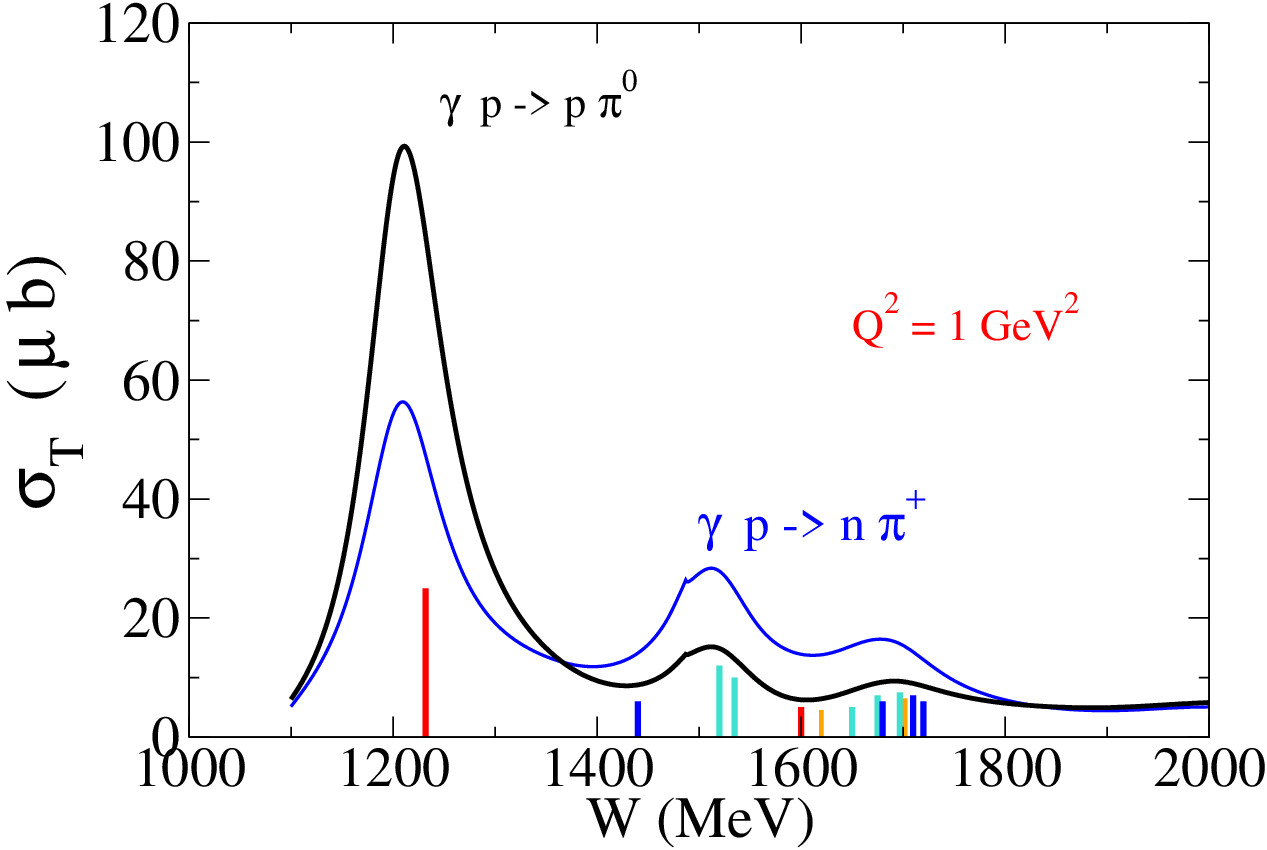
Finally, Fig. 2.1 is the classic figure that shows the consistency between the spectroscopic assignments of the lowest lying resonances and the profile of the pion photo-production transverse cross section, that clearly identifies the states in the three resonance energy regions that dominate that cross section.
2.2 Outlook: beyond the constituent quark model
Although successful, there are three problems with the quark model: the first is the old puzzle, known as the missing resonances problem [7, 9, 22, 32, 56], already mentioned in the previous sections: up to GeV about half of the states predicted by quark models was not observed or firmly established experimentally [1], even though a few new states have meanwhile been identified [6, 7]. This hints for other degrees of freedom not theoretically considered, or non dominant decays not experimentally sought (the searches were mostly restricted to scattering). Second, in the other direction, since 2015 [80] and even more recently [13] experimental evidence from the LHCb collaboration exist for non expected states or exotic states, as charmed pentaquark states which have a composition and masses 4.60 - 4.74 times the proton mass. The energies of these states are very close to the energy production thresholds of meson-baryon pairs. Finally, the third problem is that non relativistic constituent quark models do not address how the constituent quark mass emerges from the bare quark mass, i.e. the QCD feature of dynamical mass generation – which accounts for about of the light baryon masses.
All these three problems lead to the revision of the traditional quark model. Quantum Field Theory approaches become inevitable by adding particle creation and annihilation mechanisms and subsequent meson dressing extensions of the bag baryon picture. Quantum Field Theory-based functional methods of QCD as Dyson-Schwinger methods, that solve -point Bethe-Salpeter equations, have the advantage over quark models of also treating consistently both the mechanisms for quark clusterization components of the baryon wave functions, and for mass acquisition through dynamical chiral symmetry breaking.
The second problem above, on newly found multiquark compositeness (with about 30 new baryons detected by the LHC collaboration [81]) adds to the vast experimentally known complexity of meson-baryon decay channels and of electromagnetic excitations of light nucleon resonances on which we focus here. Understanding these recently found exotic tetraquark and pentaquark with significant molecular-like and/or compact structure components tests computational techniques that explain a variety of quark clusterization, and may decide on which structure (compact or a molecular-like state of five quark state?) is predominating. QCD based Dyson-Schwinger equations determine the weight in the baryon wave function of molecular-like versus compact state configurations, and the relative importance of different diquark structures [77], absent in constituent quarks traditional models. This disclosure of diquarks may shed light also on the role of collective degrees of freedom other than constituent quarks, for the solution of the first open problem above. Dyson-Schwinger equations can in principle also compare baryon components with three-quark and five-quark components.
In lattice QCD calculations it is also possible to evaluate the weight of these components, through overlaps between local three-quark interpolating fields and non local five-quark meson-baryon states. But this is less direct, and has to recur to methods as the Lüscher method for finite volume effects and comparison of effective field theory with coupled-channels results [82] (more in Section 5.4).
As a final remark: even with these advances in QCD based dynamics, a comprehensive and quantitative understanding of all observed baryon properties is not yet closed: how elementary degrees of freedom, quarks and gluons, are not observed due to color confinement remains a theoretical challenge.
3 Transition amplitudes and transition form factors
The data associated with the electroexcitation of the nucleon () can be translated into structure functions with an evolution with the invariant squared momentum transfer . The properties of these structure functions depend on the nucleon resonance , particularly on the spin-parity state . In this section we discuss the structure of the current associated with a transition, where the final state can be , , , and the initial state () is a state.
We start introducing some notation necessary for clarity of the discussion. The helicity amplitudes which parametrize the transitions in terms of the photon and nucleon polarizations are defined in Section 3.2. The transition form factors are discussed in the Sections 3.3 (for ) and 3.4 (for ). In the last case, we also define the magnetic dipole (), the electric () and the Coulomb () quadrupole transition form factors, also known as multipole form factors. The properties of the transition amplitudes at large are discussed in Section 3.5. In Section 3.6, we discuss the constraints that one needs to take into account at low , when we use either helicity amplitudes or multipole form factors.
3.1 Notation
A covariant representation is necessary throughout this review. Here we define our notation. A 4-vector is written as , where is the time component and is the space component. In general, we omit the covariant index (), unless we refer to the contravariant component . More information about the covariant notation can be found in Appendix A.
Throughout this paper, we use natural units, , with masses, 3-momenta and energies given in GeV. To convert energies in distances, we use the relation GeV fm , meaning that 1 fm GeV-1.

To describe the kinematics associated with a general electromagnetic transition, we use for the initial nucleon momentum and for the resonance momentum, as described in Fig. 3.1. We label by the reaction 4-momentum transfer and by the average of the nucleon and resonance 4-momenta
| (3.1) |
In this notation and . We denote the mass of the nucleon () by and the nucleon resonance () by .
The invariant squared momentum transfer is non positive and therefore defined in the spacelike kinematic region ()11 1 The sign of can be determined by the change of momenta in the electrons on the transition . A simple analysis of the kinematics at the Breit frame shows that , where is the 3-momentum of the final electron. Thus .. As it is usual in the literature, we define , and use the variable to parametrize the structure functions associated with the electroexcitations of the nucleon resonances. (Photoexcitations or radiative decays correspond to .)
Along this work it is useful to define two variables that will often enter into the formulas describing the helicity amplitudes, discussed next:
| (3.2) |
3.2 Helicity transition amplitudes
A general nucleon electromagnetic excitation is determined by the transition current . By definition this current encapsulates the full complexity of the vertex.
The helicity amplitudes are transition matrix elements of the projections of this current on the three possible photon polarization states. The helicity amplitudes of the transition are defined at the resonance rest frame as22 2 The amplitude is equivalent to an amplitude defined by the transition and photon polarization .
| (3.3) | |||||
| (3.4) | |||||
| (3.5) |
where is the fine structure constant, , is the photon polarization vector (), and is the magnitude of the photon 3-momentum. The current is in units of the elementary charge (). The nucleon and resonance asymptotic states have no dimensions and the helicity amplitudes have units of GeV-1/2.
The above definitions of helicity amplitudes are valid for any final state. However, the amplitude is defined only for states with . Otherwise, there are only the other two amplitudes. The scalar amplitude cannot be determined at the photon point () since there are no real photons with longitudinal polarization, but it can be measured for values arbitrarily close to .
The kinematic variables in the rest frame, with along the direction, read
| (3.6) |
where is the nucleon energy and is the photon energy. These variables can be written in a covariant form as
| (3.7) |
where for the variables defined in Eqs. (3.2) were used. The photon polarization vectors are
| (3.8) |
Differently than the longitudinal amplitudes and corresponding to photons with transverse polarization, the scalar amplitude , corresponding to photons with zero polarization, includes an extra factor to the projection . This factor is not included in some definitions of the helicity amplitudes, as for instance the helicity amplitudes in the Breit frame. Applying the current conservation condition to the product , we conclude that , i.e., the definition (3.5) is equivalent to the matrix element of the charge component of the current.
The helicity amplitudes in the limit are important for the determination of the radiative decay width of the resonances. The decay width of a resonance with spin takes the form [8, 83]
| (3.9) |
where and are the helicity amplitudes from Eqs. (3.3) and (3.4). In the case , we use .
The electron scattering on nucleons ( transitions) probe the region . Near the photon point (), the helicity amplitudes are physically defined only in the region . The minimum of is zero when the photon 3-momentum vanishes (). This point is called pseudothreshold. At the pseudothreshold the photon energy component is and . This means that, although the helicity amplitudes measured in the transitions are defined in the region , they can be extended to the region . The region can be probed by transitions, the source of the Dalitz decay (). As discussed later, the helicity amplitudes near the pseudothreshold are subject to some conditions that constraint the -dependence of those functions.

The basic ingredient of the amplitudes (3.3), (3.4) and (3.5) is the transition current which is a theoretical object. But how are helicity amplitudes extracted from the data? Since the resonances decay into baryon and meson final states, the transition current or is necessarily part of the pion photoproduction and electroproduction off nucleons. The experimentally extracted amplitudes, labeled , and , are obtained from data analyses of pion electroproduction (or meson electroproduction in general) processes represented in Fig. 3.2, where the contribution of diagram (d) has to be separated. Pion electroproduction combines a electromagnetic component (), which define the helicity amplitudes, and the component of the resonance strong decay () proportional to the pion-nucleon-resonance coupling constant [84]. The extraction of the helicity amplitudes from the pion production amplitudes depends on relative signs of the (present in the Born term) and couplings.
In Refs. [85, 86] it is shown that the theoretical calculations of the helicity amplitudes by Eqs. (3.3), (3.4) and (3.5) with the experimentally measured , and are related through a global sign
| (3.10) |
where
| (3.11) |
It is understood that and are determined by the same framework, and as a consequence the r.h.s. is independent of relative signs of the nucleon and resonance states [8, 85]. Detailed discussions on the subject can be found in Refs. [8, 85, 87].
In quark model calculations the phase between the calculated amplitudes and the measured amplitudes, which depend on the relative sign between of the resonance and nucleon states33 3 In the elastic transitions or the normalization is fixed by the charge of the baryon ( and ) and the result is independent of the sign of the normalization constant. In inelastic transition the form factors depend on the relative phase of the two states. can be determined directly by the data in the following way: one adjusts the sign of the resonance wave function by the comparison of the model calculations with the helicity amplitude data for large , where the valence quark degrees of freedom dominate and the meson cloud excitations are negligible [85, 86, 88].
In the previous discussion we gave the decay channel as an example, since it is the dominant source of information about the transition. But the analysis can include other decay modes as the channel in the state or the channel in the state [8, 9, 89, 90, 91, 92]. The implementation of the method becomes more complicated for resonances with a weak coupling to the channel or with dominance of the channels [8, 7, 90, 93].
In the next sections, we present the expressions for the helicity amplitudes based on the relations (3.3)–(3.5), and multipole transition form factors for resonances with , , . The conventions associated to the gamma matrices and the normalizations of the states are presented in Appendix A. We start writing the transition current for a resonance characterized by the spin-parity , using Lorentz structures built from the momentum variables and , compatible with gauge invariance and free of kinematic singularities [84, 94]. The transition current is then expressed in terms of independent kinematic-singularity-free form factors , which are used to write down the expressions for the helicity amplitudes and multipole form factors. We follow the formulation from Devenish et al. [84] and Aznauryan and Burkert [8], and adopt the normalization of Aznauryan-Burkert. Early formulations of transition currents can be found in Refs. [94, 95]. The results for the case and , are presented in Sections 3.3 and 3.4, respectively.
It is worth noticing that the transition form factors used in the parametrization of the transition current are kinematic-singularity-free functions and form an independent basis, meaning that they are uncorrelated and free of constraints. As for the helicity amplitudes and multipole form factors expressed in terms of the kinematic-singularity-free form factors , they are not independent in the kinematic limits , and are therefore subject to some constraints. The constraints associated to the helicity amplitudes and multipole form factors near the pseudothreshold, , below the -range reveled by electron scattering (), are discussed in Section 3.6.
3.3 Form factors
With the notation for the momenta variables of Eq. (3.1), the most general structure for the transition current associated with the vertex can be represented by the following combination of the two possible vector Lorentz structures
The previous equation describes the current associated to the states in the following way: the upper operator stands for the upper parity index () and the lower operator stands for the lower parity index (). This notation will be used along the article. The transition form factors and have dimensions of inverse of square masses ().
Another common representation of the current used in the literature [88, 96, 97, 98] is
where and are dimensionless and given by and . The form factors and are known as Dirac and Pauli form factors, respectively, as in the case of the nucleon elastic form factors. Comparing to Eq. (3.3) we notice that the Lorentz operator of the first term has a singularity at . This singularity is canceled by the factor in , leading to the constraint . The representation (3.3) has the advantage of avoiding singularities on the Lorentz structure operators. The representation (3.3) is advantageous for the comparison with the elastic limit for .
From the definitions above, we obtain the relations between the kinematic-singularity-free form factors and the helicity amplitudes introduced in the previous section for
| (3.22) | |||
| (3.23) |
with
| (3.24) |
In these and in the following formulas, we use a compact notation for the obtained signs: the upper and lower sign specifies respectively the parity index, corresponding respectively to the upper and lower operators in Eq. (3.3). The upper signs holds then for and the lower signs holds for .
The helicity amplitudes in terms of the Dirac and Pauli form factors are
| (3.25) | |||
| (3.26) |
with . In this case, we can calculate the inverse relations
| (3.27) | |||
| (3.28) |
Importantly, the determination of and data is only possible when there are data for and at the same value of . The exception is the point , where cannot be measured and , by construction. From Eq. (3.28), one has .
In the representation by the and form factors, there are no singularities in the amplitude , because in (3.26) the prefactor combines with such that in the limit the ratio converges to a constant, , and .
In the case the amplitudes take the form and , similar to the relations and for the nucleon elastic form factors [99, 100, 101]. Notice, however, that the functions and have different meanings in the case of elastic and inelastic transitions. In the inelastic transitions, one has always . In the elastic transitions this happens only for neutral baryons, as in the case of the neutron.
Some authors define the Coulomb () and magnetic/electric () form factors for the states based on the direct relations with the amplitudes and the magnetic/electric amplitudes [78, 102, 103]. One obtains then for
| (3.29) |
The combination is relabeled as Coulomb form factor [78, 102]. As for , one has
| (3.30) |
with .
3.4 Form factors
In this section, we present the formulas for the helicity amplitudes and the multipole transition form factors of the high spin cases, . These functions are also expressed in terms of independent kinematic-singularity-free form factors. For simplicity, we introduce auxiliary functions labeled as helicity form factors [84]. The explicit forms depend on the quantum number
| (3.31) |
There are similarities between the case and the cases . Notice the alternation of parity, when we increase . Because of the similarities, it is convenient to separate the case from the high order spins. Thus, in Section 3.4.1, we discuss the results for , and in Section 3.4.2, we discuss the results for .
We can anticipate that for a fixed , the transverse helicity amplitudes and the electric and magnetic form factors for negative parity states can be obtained from the formulas for positive parity through simple transformations.
3.4.1 Case
Let us start with the case for clarity. The projection of the transition current on the asymptotic states and can be expressed as
where and are the resonance Rarita-Schwinger and nucleon Dirac spinors, respectively. The operator is in units of the elementary charge (). According to the notation adopted, the upper operator is associated with the upper parity index (state ) and the lower operator is associated with the lower parity index (state ). The spin projectors of the state and of the nucleon are omitted for simplicity.
The operator can be expressed in the gauge-invariant form [8]
| (3.35) |
where are independent kinematic-singularity-free form factors. The dimensions of the form factors are , and .
Using the form factors , we can define the helicity form factors [8, 84]
| (3.36) | |||
| (3.37) | |||
| (3.38) |
For the helicity form factors are dimensionless.
The helicity amplitudes can now be calculated using
| (3.39) |
where
| (3.40) |
Again, the previous equations are valid for the states, where the upper signs hold for the upper parity index () and the lower signs hold for the lower parity index (). We use here the Aznauryan-Burkert representation [8] which is equivalent to the Devenish representation [84] when we redefine .
The multipole form factors can now be expressed in terms of the helicity amplitudes. For , one has [8, 78, 107]
| (3.41) | |||
| (3.42) | |||
| (3.43) |
and for
| (3.44) | |||
| (3.45) | |||
| (3.46) |
where
| (3.47) | |||||
The explicit expressions for , and in terms of are presented in Appendix B. The previous formulas show that we can obtain the electric/magnetic form factors for from the formulas for interchanging and .
For convenience, we also compile here the inverse relations for the helicity amplitudes in terms of the multipole form factors, for :
| (3.48) |
and for :
| (3.49) |
As a consequence, the relations between the and multipole form factors, we can obtain the amplitudes for from the formulas for replacing , and .
For the comparison with the literature we add that the formulation from Devenish [84] and Jones and Scadron [94] includes an isospin factor associated to the transition on the vertex (3.4.1) which leads to different transformations between and multipole form factors. These transformations are discussed on Appendix B. The present formulation and the Devenish/Jones and Scadron formulation are, however, equivalent, and give the same multipole form factors and helicity amplitudes (see Appendix B).
To prepare the discussion of the asymptotic behavior of the helicity amplitudes in the following sections, we present a relation between the functions and . From Eqs. (3.37) and (3.38), one obtains
| (3.50) |
and we conclude that
| (3.51) |
There are alternative representations for currents that can be generalized for [84, 108, 109, 110]. Some of the representations are presented in Devenish et al. [84] and Jones and Scadron [94]. Several authors [111, 112, 113] propose another representation which also defines three kinematic-singularity-free form factors44 4 In the original form [25, 114], the form factors have a kinematic zero at the threshold , but they can be redefined without the kinematic zero [108]. usually labeled as , and . The explicit forms and the conversion into the Jones and Scadron multipole form factors , and can be found in Refs. [25, 108, 114]. A difference to the form factors , and , defined above, is that , and are correlated at large [108]. Pascalutsa and Vanderhaeghen have used extensively this representation within the chiral effective field theory and large limit frameworks in calculations of transition form factors [40, 114, 115, 116], two-photon contributions to transition form factors [117] and in the Compton scattering [25, 112]. The modified parametrization from Ref. [108] has shown to be particularly appropriate for the study the falloff of the transition form factors with and for the calculation of the nucleon resonance contributions to the nucleon Compton scattering. The transition form factors have monotonous falloffs with , except for radial excitations, where we expect some zero crossing [108]. Another representation for transition to states proposed by Vereshkov and collaborators [109, 110], uses simple linear combinations of the kinematic-singularity-free form factors . This representation has some advantages in the study of the asymptotic behavior of the multipole form factors [109, 118, 119].
3.4.2 Cases ,
For the states , (), the transition current reads [8]
where takes the form (3.35) and is in units of the elementary charge (). The states are discussed in Appendix C.
Equation (3.4.2) is valid within the adopted notation: the upper operator holds for the states , and the lower operator holds for the states , . It is important to realize that in Eq. (3.4.2) the effective vertex for includes, in addition to , the momenta , and differ from the case in the dimensions of .
The expressions for the helicity amplitudes associated with the states , , can be written using Eqs. (3.36)–(3.38) as
| (3.55) |
where
| (3.56) |
The upper signs hold for the states , , and the lower signs hold for the states , (). The same sign convention is used in the functions defined by Eqs. (3.36)–(3.38). The expressions presented above are calculated directly from the definitions (3.3)–(3.5) using the spin spinors associated to the resonances. The factor entering in the amplitude is a product of Clebsch-Gordan coefficients for the states55 5 Given , we can write , where is the product of Clebsch-Gordan coefficients : and can be written in the form
| (3.57) |
From the previous relations, we can conclude that the helicity amplitudes can also be written in terms of the helicity form factors , defined previously for , with the conversion factors depending on . This dependence appears on the factor for all the amplitudes and on the factor for .
Differently than for , the helicity form factors have now dimensions , since has dimensions , and the helicity amplitudes have dimension . The kinematic-singularity-free form factors carry the dimensions , and , and the multipole form factors , and discussed next, have also dimensions .
For a compact and simple representation of the multipole form factors, we define
| (3.58) | |||||
For , we obtain
| (3.59) | |||
| (3.60) | |||
| (3.61) |
| (3.62) |
For , one has
| (3.63) | |||
| (3.64) | |||
| (3.65) |
| (3.66) |
Again, negative parity amplitudes can be obtained from positive parity amplitudes by replacing , , and . The explicit expressions for , and in terms of the kinematic-singularity-free form factors are presented in Appendix B.
The relations presented here for the helicity amplitudes, multipole form factors and the conversion relations are also valid for the particular case (). The separation in the cases and is justified by the need to emphasize the differences associated with the use of spinors with indices (see Appendix C). The more relevant differences come from the inclusion of factors depending on in the expressions for the multipole form factors and the phase .
The relations (3.59)–(3.60) and (3.63)–(3.64) for the multipole form factors are in agreement with the radiative decay widths from Devenish et al. [84, 102], for a generic resonance of spin , and with Eq. (3.9). The results for the helicity amplitudes and for the conversion helicity amplitudes/multipole form factors differ from Aznauryan-Burkert [8] for (). The differences are in the phase , absent in Aznauryan-Burkert, and in the factor for . Notice, however, that the radiative decay widths are insensitive to the signs of the helicity amplitudes.
From the theoretical point of view, the multipole form factors for are very convenient for the study of the large- region due to the correlations between electric and magnetic transition form factors. These correlations can be deduced from the helicity amplitudes (3.48), (3.49), (3.62) and (3.66), and is discussed in the next section.
3.5 Large
The behavior of the helicity amplitudes and multipole form factors can be estimated in the perturbative QCD (pQCD) regime when is very large [120, 121, 122, 123, 124, 125]. These estimates use hadron helicity conservation and dimensional counting rules related to the effective number of quarks or antiquarks [102, 122]. The calculations assume that at very large the photon momentum is redistributed by the three quarks (the dominant Fock state) through two gluon exchanges. The explicit calculations require the use of distribution amplitudes derived from pQCD which include the three quark component of the baryon wave functions at short distances [122, 123, 125]. Estimates of the helicity amplitudes for the and systems at large [126, 127, 128] are discussed in Sections 6.2 and 6.3, respectively.
3.5.1 Breit frame amplitudes
The analysis of the asymptotic or pQCD results is simplified when one uses the Breit frame (BF), where , and the subscripts stands for Breit frame.
Choosing the 3-momentum of the resonance along the axis, one can write , , where , , and . The momentum transfer is then , where .
The Breit frame is useful to study the large- limit because it maximizes the 3-momentum transfer: for large the energy component is suppressed (), while . For comparison with the rest frame, the relation between the magnitude of the photon 3-momentum in the two frames is .
In the Breit frame, we can define the three amplitudes [126]
| (3.67) |
where labels the photon polarization (), and represent the final and initial helicities, respectively (recall that the initial state has momentum , consequently the spin projection in the direction is ). In comparison to the formulas by C. Carlson et al. [126], in these definitions we have omitted the factor .
The explicit form for the three possible amplitudes take the form [124, 126, 129]
| (3.68) | |||
| (3.69) | |||
| (3.70) |
Note that the previous relations resemble the amplitudes (3.3), (3.5) and (3.4) when we use the spin projections and . The main difference is that is not modified by the factor , like .
Since the amplitudes at the Breit frame (3.68), (3.69) and (3.70) and the amplitudes at the rest frame (3.3), (3.5) and (3.4) can both be expressed in terms of the kinematic-singularity-free transition form factors (Sections 3.3 and 3.4), one can relate the two sets for the cases , , , by
| (3.71) |
The amplitudes and are not defined when . As before, we use the upper symbols for the states , , and the lower symbols for the states , , . The sign in the amplitudes and follows from the properties of the space reflection of the states in rest frame and in the Breit frame [130].
For completeness, we mention that some authors [125] define also helicity amplitudes at the Breit frame , and using () and , where . In this case, we obtain the correspondence () and , where .
3.5.2 Asymptotic behavior
The calculation of the leading order dependence on of the Breit frame amplitudes by C. Carlson et al. [124, 127, 128] shows that the dominant amplitude at large is the amplitude , which preserves the helicity. For large , one has . The calculations show also that each flip of the helicity of a quark introduces a suppression of the amplitudes by a factor . The expressions for the amplitudes for large in leading order can then by written as [126, 129]
| (3.72) |
Combining the relations (3.71) and (3.72), we conclude that
| (3.73) |
using the relation for large .
In the derivation of the relations (3.72) and (3.73) only the leading order dependence on has explicitly been taken into account. Smother contributions related to logarithmic corrections from different sources are omitted in the previous relations. As a consequence, the relations (3.72) and (3.73) are valid only apart log corrections (modulo logarithms) [126, 129].
The logarithmic contributions to the leading order power laws (3.72) and (3.73) have different sources, and can be expressed in terms of powers of , where is a soft pQCD scale [122, 125, 131]. The scale is a low-energy regulator associated with the size of the baryons, and has typical values of 0.2–0.3 GeV [125, 131, 132]. The logarithmic corrections are due to the strong running coupling constant in the form [122, 123, 124, 125, 131, 133], to soft contributions associated to the light cone distribution amplitudes of the baryons [122, 123, 125, 134], and also due to the regularization of the divergent integrals with the introduction of a low-energy cutoff [131, 132]. The global logarithmic calculations can be determined analytically for the nucleon elastic form factors [122, 123, 131], but are very sensitive to the light-cone distribution amplitudes for the transition form factors [134]. The study of leading order dependence of the form factors (3.72) or helicity amplitudes (3.73), can be improved when we scale the data by for a given scale , or when we consider ratios between form factors or helicity amplitudes. This way, we eliminate the global logarithmic effect of the strong coupling constant [118, 119, 123, 131, 132]. In the following, we assume that apart the global factor , the logarithmic corrections are similar for all Breit frame amplitudes, , and , and correspond to smooth functions that can be regarded as constants in a first approximation.
The expressions for the helicity amplitudes (3.73) can be transposed for the form factors, modulo logarithm. In the case , we can use (3.27) and (3.28) to conclude that
| (3.74) |
In the case the asymptotic behavior of the form factors and , can be derived from the relations between helicity amplitudes and form factors (presented in Appendix B). The results for are
| (3.75) | |||
| (3.76) | |||
| (3.77) |
The details of the calculations are in Appendix D. As for the helicity amplitudes, the above relations are valid apart logarithmic corrections.
The relations (3.73) have been tested at the maximum values of available for the resonances , , , and up to , 6 or 7 GeV2, depending on the case. In Fig. 3.3, we present the experimental data for the amplitudes and for the mentioned resonances, multiplied by the factor . The graphs show a trend compatible to a constant in the range –4 GeV2, as suggested by Eqs. (3.73), although the error bars are large for the amplitude [8]. Future data from JLab-12 GeV or future JLab updates [7] may help to confirm this trend. The large behavior of the resonances , and are discussed in detail in Sections 6.2, 6.3 and 6.4, in that order.
We do not present the test for the amplitude , expected to scale with , since the results for the , for and are less conclusive for different reasons. In the case of the , the uncertainties are large. In the case of the , the present data suggests that the convergence may happen only for very large , as discussed in Section 6.3.


The study of the asymptotic behavior can be very interesting when we use the multipole form factors (3.77). According to Eqs. (3.48) and (3.49) the results and are equivalent to
| (3.78) |
This large- relation is valid in particular for the and states.
The correlations between electric and magnetic form factors can also be observed for higher spin resonances . We use again . The explicit form can be derived from the relations (3.59)–(3.61) and (3.63)–(3.65) and the asymptotic forms and . One has then for ,
| (3.79) |
and for the cases ,
| (3.80) |
It is important to mention, however, that the relations (3.72) and (3.77) are derived under very general assumptions. One important assumption is that the kinematic-singularity-free form factors are non zero. A simple illustration of a deviation from the expected leading order behavior can be obtained for instance for the resonances if . According to the relations (3.51), if vanish, we would have for , and for . As a consequence, from Eqs. (3.48) one obtains the relation , in contradiction with the relations (3.73) for . This illustrates that deviations of the general power laws in some particular cases can be expected.
The study of the falloff tail of transition form factors and of the helicity amplitudes at large is important because it enables us to deduce the contribution from higher order Fock states, namely the ones associated to quark-antiquark excitations. At very large , one expects the leading order form factors for and for to be dominated by terms on , where is the number of effective constituents [126, 128]. The power of the asymptotic falloff is associated with the minimum number of gluons exchanged between the constituents. When the change from (falloff ) to a system of three quarks and a quark-antiquark pair, one has 5 constituents (), and expect than that the asymptotic behavior follows . The price of the change from to is then the extra suppression. The previous estimate can be generalized for next leading order form factors (, and ) accounting for the faster falloffs (, , etc.). The test of the asymptotic behavior of the amplitudes or of the multipole form factors can then be useful to establish the range where the valence quark degrees of freedom start to dominate, since the relations are based on the properties of the valence quarks.
Concerning logarithmic contributions to the leading order from Eqs. (3.73), there are attempts to parametrize these corrections by Vereshkov and collaborators [109, 110]. We notice, however, that although the corrections may be relevant for some amplitudes, to find their explicit experimental signals may require much larger values for and broader distributions of data.
3.6 Empirical parametrizations of the helicity amplitudes
In theoretical and phenomenological calculations, it is convenient to use parametrizations of the data obtained for the helicity amplitudes or for the transition form factors (, and for , and , or for ) based on simple analytic functions of . Examples of successful parametrizations of the data are the MAID parametrizations [78, 137, 138], rational parametrizations [108], parametrizations based on the JLab/CLAS data for the resonances and presented in Refs. [8, 89], and more recently a complete set of parametrizations of 12 states below 1.8 GeV associated with states , and based on JLab/CLAS data [139]. A collection of the JLab/CLAS data and relevant data from other groups can be found in Ref. [140].
In this section, we discuss the constraints on the helicity amplitudes and transition form factors that should be taken into account near the pseudothreshold, where the photon 3-momentum vanishes and . As discussed in Sections 3.3 and 3.4, the helicity amplitudes and the multipole form factors are linear combinations of the unconstrained kinematic-singularity-free form factors . Near the pseudothreshold, however, there are constraints on the helicity amplitudes and the multipole form factors, which cannot be ignored when we consider empirical parametrizations of these structure functions. However, some phenomenological parametrizations of the data ignore those constraints at low , and end up with -dependencies incompatible with the pseudothreshold constraints. The impact of the constraints on phenomenological parametrizations of the data may be especially significant for light nucleon resonances because the pseudothreshold is very close to the photon point . When the parametrizations are implemented on the kinematic-singularity-free form factors or an equivalent kinematic-singularity-free basis, the pseudothreshold constraints are automatically satisfied [108, 141]. An example of such phenomenological parametrization is in Ref. [108].
The constraints on the helicity amplitudes and multipole form factors are a consequence of the structure of the transition current and its behavior near the pseudothreshold [84, 94, 95]. The gauge-invariant structure of the transition current , based on the independent kinematic-singularity-free form factors , and the kinematics in the rest frame imply that the helicity amplitudes near the pseudothreshold must have an explicit dependence on , and also that some amplitudes are correlated [142, 143, 144, 145, 146].
The leading order dependence of the helicity amplitudes in terms of can be derived from Eqs. (3.22), (3.23) and (3.24) for , and Eqs. (3.39), (3.40), (3.55) and (3.56) for , combined with the fact that the form factors are free of singularities (finite and well defined functions in the limit ). Noticing that for small , based on Eq. (3.24), we can write and , we conclude that the leading order dependence of the amplitudes and corresponds to the expressions displayed in the first and second columns of Table 3 for . From Eqs. (3.40) and (3.56), we can also conclude for that and for small . Using these relations for , we conclude that for , , , one has
| (3.81) |
and for , we obtain
| (3.82) |
The leading order dependencies for are also presented in the first and second columns of Table 3.
The most well known effect related to the constraints at the pseudothreshold is known as Siegert’s theorem or long wavelength theorem [142, 143, 144, 145, 146, 147]. The theorem states that the scalar amplitude and the electric amplitude (combination of the transverse amplitudes and ) are related by . A simple consequence of this relation is that the scalar amplitude (), where represents the projection of between equal spin projections states (), vanishes when . The condition , when both states are at rest (), is equivalent to the orthogonality of the and states [148, 149]. The explicit relations between the scalar amplitude and the electric amplitude, expressed in terms of and , are presented in the third column of Table 3. For the state there is no relation associated to Siegert’s theorem, because the electric amplitude is not defined [78, 84, 102]. At this respect, recall the discussion at the end of Section 3.3. In addition to the correlation between electric and scalar amplitudes, in the cases , there is also a correlation between the transverse amplitudes and , equivalent to the condition that the magnetic amplitude vanishes at the pseudothreshold. This condition is included in the last line of the third column of Table 3, for and for
| , | ||||
|---|---|---|---|---|
| , | ||||
| , | ||||
| , | ||||
| , | ||||
| , | ||||
The correlations between amplitudes can be converted into correlations between multipole form factors, using the conversion formulas of the previous sections. The condition associated with Siegert’s theorem leads to relations between the electric and Coulomb quadrupole form factors [84, 94, 95]. The explicit expressions are displayed in the fourth column of Table 3. The condition for is also the consequence of the definitions (3.30) [103]. The relations for are equivalent for the states . Similarly, the relations for are equivalent for . The relation for the magnetic form factor for is also valid for the states . In this case the relation between the transverse amplitudes can be written in the general form . The relations for the multipole form factors can be also derived from expressions for the multipole form factors in terms of the form factors , presented in Appendix B, considering expansions in powers of [150]. In the following, and along the article, we focus on the parametrizations for . In the states with the pseudothreshold is more distant from the photon point, and there is also a lack of data below GeV2 [140].
A note on the possible analytical form of the helicity amplitudes is in order. Parameterizations based on smooth analytical forms, like rational functions, may not be appropriate for the transverse amplitudes of the excitations of and , even when compatible with the pseudothreshold constraints [141]. This happens because of the proportionality to , due to the difficulty of approximating the factor by a rational function, for light resonances (small ). Recall that near the pseudothreshold . This effect is illustrated in Section 6.3.4 for the helicity amplitudes.
As mentioned, the constraints described above are not always considered in parametrizations of the data, that erroneously considered the amplitudes as independent functions in the whole region of . Even the parametrizations developed by the MAID group [78, 137, 138], that take into account some features of the helicity amplitudes [151, 152, 153], with particular emphasis on the relation (Siegert’s theorem), fail in obtaining parametrizations fully consistent with the pseudothreshold constraints, and some of the relations displayed in columns one, two, three and four of Table 3 are violated. The MAID parametrizations are in general compared with the MAID data analysis from different groups, as described in Refs. [78, 137, 138]. We refer to this MAID data analysis, collected in the website [154], as MAID data. Some of these issues are discussed by Tiator in Ref. [153] within the context of the MAID parametrizations.


Reprinted with permission from L. Tiator, Few Body Syst. 57, 1087 (2016). Copyright (2016) by Springer.
The results of the MAID parametrization for the amplitude for the states and are presented in the upper panel of Fig. 3.4 (solid lines). The results are compared with the estimate given by (dot-dashed lines) according with the results from Table 3. At the first glance, the figure suggests that Siegert’s theorem is verified in the case of the , since the two lines converge at the pseudothreshold, and that there is a clear violation of the theorem for , since the parametrization fails to reproduce . In the case of the , a closer look reveals that the two calculations have different derivatives. This means that, although the amplitudes and have the correct shape at pseudothreshold ( and ) the relation between the amplitudes is not consistent with the condition , displayed on Table 3. Notice the importance of including the factors and . The condition for the form factors (fourth column) is equivalent to the condition for the amplitudes, only when the amplitudes scale with the correct power of [149, 150].
In the lower panel of Fig. 3.4, we present calculations of the and amplitudes compatible with Siegert’s theorem. In the case of the (left panel), we include calculations of a quark model which take into account pion cloud contributions for the form factors and valid in the low- region [148, 155, 156]. The results are consistent with the relation per construction [148], and satisfy consequently the equivalent relation for the amplitudes. The results for the at low are discussed in more detail in Section 6.3. The results for the presented on the right panel are obtained using a parametrization based on a MAID form that take into account the expected shape for and the constraint associated with Siegert’s theorem (see Table 3). The free parameters are fixed by the MAID data [149]. The new parametrization reveals a turning point in the function near the pseudothreshold [149], as a consequence of the positive values for the function and Siegert’s theorem condition. The properties of the helicity amplitudes at low are discussed in detail in Section 6.2. The impact of the pseudothreshold constraints on other resonances are discussed in Section 6.
The discussion of this section answers the question about how to test the consistence of the parametrizations with the pseudothreshold constraints. Another possible question is, given a set of parametrizations of the helicity amplitudes for a resonance in a certain range of , but incompatible with the pseudothreshold constraints, if it possible to make it compatible below a given value of . This subject was discussed in Ref. [141], where a method is proposed to extrapolate parametrizations defined for , below a point to the pseudothreshold, using smooth analytic extensions of the original parametrizations, while ensuring them to be consistent with the pseudothreshold conditions. The method was applied to the JLab parametrization [139, 157], but it can be applied in any analytic parametrizations of the nucleon resonance helicity amplitudes. Examples of the method are discussed in Sections 6.2 and 6.3 for the cases of the and . The state turns out to be a special case where low- data are crucial to establish the sign of the amplitudes and near , as discussed on Section 6.2.3.
| Reaction | (GeV2) | Functions | Lab/Experiment | |
|---|---|---|---|---|
| 2.4, 3.6 | JLab/Hall C [158] (1999) | |||
| 1.8–4.0 | JLab/CLAS [159] (2001) | |||
| 0.17–3.1 | JLab/CLAS [91] (2007) | |||
| 5.7, 7.0 | JLab/Hall C [92] (2009) | |||
| 0.38, 0.75 | , | JLab/CLAS [160] (2005) | ||
| 0.40, 0.65 | , | JLab/CLAS [160] (2005) | ||
| 0.40, 0.65 | , , | |||
| 0.40, 0.65 | , | |||
| 0.3–6.0 | , , | JLab/CLAS [89] (2009) | ||
| 0.30–4.16 | , | |||
| 0.30–4.16 | , , | |||
| 0.30–4.16 | , | |||
| 1.8–4.0 | , , | JLab/CLAS [161] (2015) | ||
| 1.8–4.0 | , , | |||
| 1.8–4.0 | , | |||
| 0.1 | MAMI-A1 [162] (2017) | |||
| 0.65 | , | JLab/CLAS [163] (2005) | ||
| 0.65 | , , | |||
| 0.28–0.58 | , | JLab/CLAS [90] (2012) | ||
| 0.28–0.58 | , | |||
| 0.65, 0.95, 1.30 | , | JLab/CLAS [164] (2014) | ||
| 0.65, 0.95, 1.30 | , , | |||
| 0.65, 0.95, 1.30 | , , | |||
| 0.65, 0.95, 1.30 | , | JLab/CLAS [93] (2016) | ||
| 0.65, 0.95, 1.30 | , , | |||
| 0.65, 0.95, 1.30 | , | |||
| 0.65, 0.95, 1.30 | , | JLab/CLAS [165] (2020) |
| Reaction | (GeV2) | Functions | Lab/Experiment |
|---|---|---|---|
| 0.0 | MAMI [166] (2000) | ||
| 0.0 | LEGS [167, 168] (2001) | ||
| 0.127 | ELSA [169] (1997) | ||
| 2.8, 4.0 | , , | JLab/Hall C [136] (1999) | |
| 0.121 | MAMI [170] (2001) | ||
| 0.4–1.45, 1.8 | , | JLab/CLAS [171] (2002) | |
| 0.126, 127 | , | MIT-Bates [172, 173] (2003) | |
| 0.127 | , , | MIT-Bates [174] (2005) | |
| 0.06, 0.200 | , , | MAMI-A1 [175, 176, 177] (2008) | |
| 1.0 | , | JLab/Hall A [178, 179] (2007) | |
| 0.127 | MAMI-A1 [180] (2013) | ||
| 0.09, 0.13 | JLab/Hall A [181] (2016) | ||
| 0.04, 0.09, 0.13 | JLab/Hall A [181] (2016) | ||
| 3.0–6.0 | , , | JLab/CLAS [182] (2006) | |
| 0.16–0.28 | , | JLab/CLAS [89] (2009) | |
| 0.30–1.45, 3.0–6.0 | , , | JLab/CLAS [89] (2009) | |
| 6.4 | , , | JLab/Hall C [135] (2009) | |
| 7.7 | JLab/Hall C [135] (2009) |
4 Experimental facilities and methods of analysis of the data
In this section we discuss the experimental facilities and methods used in the analysis of the data. We start with the list of current experimental facilities dedicated to study of the electromagnetic structure of the nucleon resonances in the spacelike region, and with large contribution to the knowledge of the properties of the resonances and helicity amplitudes. Next, we discuss the methods used in the analysis of the data for the determination of the properties of the baryon resonances. The properties, discussed here include pole positions, resonance masses, decay widths, and branching ratios. To close the section we discuss the class of models for the meson-baryon interaction known as dynamical reaction models, which are used in the analysis of the meson electroproduction data.
4.1 Experimental facilities
The Thomas Jefferson National Accelerator Facility (JLab for short), located in Newport News (USA), and known before 1996 as the Continuous Electron Beam Accelerator Facility (CEBAF), operates a continuous wave electron accelerator in the luminosity frontier, that already for about two and a half decades produces the highest intensity electron beam [7, 8, 9, 10, 183]. Till 2014 the maximum energy attained by the electron beam was 6 GeV. In 2014 the energy was extended to 10.5 GeV. The extension to a beam of 12 GeV started in 2018. The first results from the JLab-12 GeV upgrade were published in 2022 [7, 11]. Under study is the extension of the JLab-12 GeV program to JLab-22 GeV [11, 183].
In parallel to the program, we notice that JLab conducted as well a variety of important experiments, as the precise measurements of the proton form factor at low , of neutron radii in nuclei, and of quark distribution functions from 3He and 3H targets. For a complete review on past achievements and future possibilities enabled by large luminosity and acceptance power consult Ref. [183]. At JLab the beam produced in the main accelerator is distributed by four main experimental Halls where the collision with the targets and the interaction with a multitude of detectors happens. The first Halls are labeled as Hall A, B and C. Hall D was built on 2014. The properties of the different Halls are described below.
Other laboratories that are also mentioned here are ELSA and MAMI (Germany) and MIT-Bates (USA), which produced relevant studies of nucleon resonances at low energy and low .
4.1.1 JLab - CLAS (Hall B)
The Hall B of JLab houses the CEBAF Large Acceptance Spectrometer (CLAS) detector, and was key for the development of the nucleon resonance program focused on the measurement of transition form factors in the first three energy resonance regions [8, 10].
This detector can operate with electron beams or with energy tagged photon beams for meson electro- and photo-production, and was designed specifically for the detection of multiparticle final states [9]. The protons and pions can be separated according to their momentum within certain limits. The identification of particles over a wide range of resonance energies () allows the study of a complete set of reactions important to the program. JLab/CLAS contributed with about 95% of the data associated with different resonances as can be inferred from the analysis of Tables 4 and 5. JLab/CLAS, now JLab/CLAS 12 is the most complete and advanced facility in the field [9]. A small caveat of the CLAS detector is the impossibility or measuring observables below GeV2.
4.1.2 JLab - Hall A
4.1.3 JLab - Hall C
The JLab/Hall C has a high momentum spectrometer. One of the applications of this detector was the measurement of and transitions at large , up to 5 or 8 GeV2 depending on the resonance. At such large values of it is not possible to separate the effects of the different amplitudes but it is possible to extract the leading order amplitude or form factor [92, 135].
4.1.4 ELSA, MAMI and MIT-Bates
Examples of electron accelerators different than CEBAF are MAMI (Mainz, Germany), ELSA (Bonn, Germany) and MIT-Bates (USA) [9].
The MIT-Bates is a linear accelerator which has been used for the study of the decay. The facility is no longer in use [8] but was decisive in the study of the quadrupole form factors at very low [175, 184].
4.1.5 LEGS (Brookhaven National Laboratory)
Of interest are also LEGS experiments at Brookhaven National Laboratory (USA) in the region at the photon point ( transition) which provided one of the first accurate measurement of the ratio .
For a more detailed discussion of these and other experimental facilities check Ref. [9]. The facilities mentioned above were focused on the study of transitions, with emphasis to the reactions , , .
4.2 Methods of analysis of the data
We discuss now methods for the analyses of the different transitions , where and are the final meson and baryon states, respectively. Originally the methods have been developed for the final state, but can be generalized for other combinations, such as , , , etc. [8, 9]. The combined analysis of different channels is important to determine the properties of the states which couple weakly to [185]. When we increase the energy of the system we open the possibility of creation of particles with strange quarks, starting with the channels , , , etc. [7]. The generalization of the method for three-body final states (two mesons and a baryon) is straightforward [9]. The analysis from JLab/CLAS of the transitions is an example of the generalization of the method [90, 93]. At the present the analyses of MAID, ANL-Osaka and Jülich-Bonn groups include states with three-body final states. In ANL-Osaka, ANL stands for Argonne National Laboratory.
The analysis of nucleon resonances was initiated by scattering studies of the transition alone, and most of the methods of analysis were based on resonance decays into the and channels. This is why till very recently the states were labeled by the properties of the decay channel using the old spectroscopic notation described in Section 2.1.2. The complexity of the analysis of the data beyond the channel comes from the resonance not being the only resonance to be taken into account, as Fig. 2.1 illustrates. Although for GeV the resonance is clearly isolated in energy, spin and parity, and the interference of the resonance with the background is then residual, the resonances from the second and third resonance region are very close to each other and effects from states with similar mass have to be disentangled [8, 9, 24]. Going beyond the channel made then necessary the simultaneous analysis of different resonance production reactions, and instead of the old spectroscopic notation, the good quantum numbers are used to classify the resonant states and [1]. Theoretically, these good quantum numbers of the three quark states come from the invariance of the QCD Lagrangian under the Poincaré group which consists of translations, rotations, boosts and parity. Nevertheless, since each and state, can be decomposed into multipole amplitudes for a reliable identification of the properties of the different and states, it is necessary to make an analysis based on a partial wave decomposition, which extracts the partial wave amplitudes (PWA) associated to the possible meson-baryon channels [9, 24, 186].
In addition, a significant information about the nucleon resonances comes also from the analysis of meson production on nucleons induced by photons. Meson photoproduction gives information beyond the scattering, in particular on states that couple weakly to the channel. A high quality data set is already available (for a review check Ref. [187]). Recently a large variety of reactions, has been investigated for increasing values of [24]. The analysis of those experiments includes not only specific masses of the nucleon resonances but also photo and meson decay widths. Although the experiments do not probe the nucleon resonances for non zero photon virtualities, the PWA of those experiments provide constraints on the position of the resonance poles which can then be analyzed in more detail in electroproduction experiments.
The study of the tied to transitions, where and are generic meson and baryon states, can be done in general through the scattering -matrix formalism. The -matrix framework is derived from the scattering matrix (-matrix) under the requirements of Unitary, Analyticity and Crossing Symmetry (symmetry between - and -channel) [9, 24, 78]. For a detailed discussion of the - and -matrix formalism we recommend Ref. [24]. The -matrix elements are projected into the possible , and initial and final states, generating a system of coupled-channel states. The explicit calculation of the and matrix elements can be done directly with the resolution of coupled-channel integral equations. In alternative, there are methods based on the -matrix, discussed below, which avoid the use of integral equations.
The -matrix formalism can be implemented using either Hamiltonian or Lagrangian formulations [8, 9, 25, 188, 189, 190], and data analysis models discussed below apply effective Lagrangians to describe the meson-baryon interactions. The interactions between baryons and mesons, defined by a Lagrangian at tree-level, are used to calculate contributions from the background and explicit contributions from the resonances in terms of the asymptotic states . Details can be found in Section 4.3. The model analysis provides a partial wave decomposition of the data with defined total angular momentum and parity (). The resonant states or are identified by the poles of the -matrix elements in the complex plan of the variable . These poles determine the resonance mass and total decay width in the formula .
Furthermore the PWA of a given or state generates an explicit multipole decomposition, and thus identifies transverse amplitudes and , which can be associated to magnetic and electric amplitudes, and scalar amplitude , which are correlated to the longitudinal amplitude through gauge invariance66 6 The current conservation condition implies that , using the rest frame representation for : .. The labels are related with the spin of the final state, according to . The multipoles , and are complex functions and are traditionally defined at the resonance rest frame where . The resonance rest frame is defined by the center of mass frame of the system. The transition form factors are determined by the imaginary part of the amplitudes , and at the resonant mass [9, 78]. In more simplified models the poles of the multipole amplitudes are introduced apriori through a Breit-Wigner form, but they can also be generated naturally by amplitudes determined by some dynamical reaction model, as discussed in the next sections.
The first analyses of the photo- and electro-production of pions on nucleon were based on dispersion relations [8, 9, 144, 186, 191, 192, 193, 194]. More recently, the analyses of the data have been done preferentially with -matrix methods [151, 195, 196], and dynamical reaction models. The -matrix formalism relation with the -matrix: , where is a hermitian operator (). The matrix elements of are necessarily real in order to preserve the unitary of the -matrix. In the practical applications, however, additional restrictions are imposed to the -matrix in order to simplify the calculations and preserve the necessary properties of the - and -matrices.
In a particular model known as the Unitary Isobar Model (UIM) [8, 9, 151], the background is unitarized for each multipole amplitude using the -matrix representation, with the resonance contributions written in Breit-Wigner energy dependent forms. The SAID, MAID, and JLab/CLAS groups have applied different forms of UIMs .
Representative groups that developed for the analysis of the reactions , and are discussed next.
4.2.1 SAID analysis
SAID (Scattering Analysis Interactive Dial-in) [79, 197, 198, 199, 200, 201, 202] is the name of the analysis performed at George Washington University (GWU) group (USA). It is characterized as a -matrix approach multi-channel analysis and is focused on the pion nucleon scattering and pion photoproduction data [8, 9, 24]. It uses polynomial parametrizations of the -matrix elements with masses, widths and hadronic couplings from pion induced production reactions and [197, 200, 202]. Photocouplings are obtained from photoproduction reactions.
Although the SAID analyses are not applied directly to the transitions, their results for and are used as reference of several groups, including the MAID, ANL-Osaka, Jülich-Bonn and Kent University State analysis [24], discussed in the following sections.
4.2.2 MAID analysis
MAID (MAinz unitary Isobar moDel) is the analysis developed by the Mainz group (Germany) [78, 137, 138, 198, 203]. As the name suggests it is based on an UIM as defined in Ref. [151].
The MAID analysis is applied to the and reactions. Thus, the MAID model is not a coupled-channel analysis in the sense that does not go above the channel. The inclusion of other channels has been considered in specific applications of MAID, including the Eta-MAID, Kaon-MAID and EtaPrime-MAID [203, 204].
The -matrix for the transition takes the form [25, 78, 137, 138]
| (4.1) |
where is the scattering matrix ( transition), is the transition potential, and is the free propagator, as defined in the Lippmann-Schwinger formalism. The integration in the intermediate momenta is implicit in Eq. (4.1). In the present notation stands generically for the channel for both real and virtual photons.
The MAID analysis decomposes the interaction term into background (bg) and resonant (R) contributions
| (4.2) |
The potential is described by the Born terms including a mixture pseudoscalar-pseudovector coupling and -channel vector meson exchanges. The term includes the bare contributions of the resonance.
From Eqs. (4.1) and (4.2), one concludes that [78, 205]
| (4.3) |
where
| (4.4) | |||
| (4.5) |
In this representation and are both unitary. From Eqs. (4.4) and (4.5), we conclude that the background and resonant contributions can be determined once the scattering matrix is known. Notice also that comprises contributions from both the background and the resonances since the amplitude includes all the mechanisms [8, 78].
The previous relations define what is known as the Dubna-Mainz-Taipei (DMT) model [205, 206]. The MAID analysis differs from the DMT model in the amplitude defined by Eq. (4.4). Instead of considering the explicit integration, the determination of the background contributions as in the original UIM [138, 151], replaces the explicit integral in Eq. (4.4) by the term of the elastic cut only, neglecting the contribution from the principal part of the integration [9, 78]. This procedure gives for the MAID contribution of the background [78, 151]
| (4.6) |
where the amplitude is the on-shell pion-nucleon elastic amplitude, as determined by SAID in terms of phase-shifts and inelasticity parameters [24, 78], and specifies the orbital angular momentum (), the total angular momentum (), the isospin (), and the multipole label . The dependence on is included explicitly.
As for the resonant term, MAID considers an energy dependent Breit-Wigner type amplitude parametrization
| (4.7) |
where are resonance R electromagnetic couplings, labels the multipoles (), and are the mass and total decay width of the resonance respectively, and are known parametrizations associated to the radiative decay and decay in terms of the energy , and is a phase necessary for the unitarization of the amplitudes [24, 78, 204]. Its explicit form can be found in Refs. [8, 78, 138]. The contribution of all intermediate resonance is summed over to make the total resonant contribution.
For the determination of the transition form factors it is important to discuss the form of the amplitudes . The MAID parametrization of the amplitudes takes the general form
| (4.8) |
where () and are adjustable parameters. For most resonances, MAID considers determined by the value of at the pole [24]. This combination of polynomials and exponential functions provides a simple and economical way (due to the reduced number of parameters) to describe functions of , which may have complicated shapes. In the case of the resonance, some multiplicative functions are also considered, including the dipole function , where GeV2, and a factor , where is the magnitude of the photon 3-momentum and [78]. The inclusion of these factors is important to ensure consistency with the constraints at the pseudothreshold, particularly for the case of the , as discussed in Section 3.6. The inclusion of similar factors for other resonances is under consideration [141, 149, 150, 153].
The MAID parametrizations (4.8) deserve some discussion. Extrapolations for should be taken with caution due to the possibility of significant exponential enhancement. It is assumed that the parametrizations are limited to a certain range of determined by the available data. The upper range can then be 4.5 or 8 GeV2 depending on the resonance. One notice, however, that the expected asymptotic large- dependence (see Section 3.5) are not considered in the MAID parametrizations. As an example, notice that the form factors and are in general regulated by different values of , thus implying a dominance of one over the another for very large . In any case, the asymptotic behavior of the MAID parametrization can be redefined above a certain limit if necessary. A discussion of the modification of the MAID exponential shape of amplitudes for large can be found in Ref. [150].
4.2.3 JLab/CLAS analysis
The method used by the JLab/CLAS group, sometimes mentioned as the JLab/Yeveran model [9] is a model that combines fixed- dispersion relations with a UIM in the form proposed by Drechsel et al. [151]. The UIM method is extended with the incorporation of Regge poles for the large- region [8, 191]. The approach is described in detail in Refs. [160, 163, 191].
The comparison between the two separate approaches, dispersion relations and extended UIM, allowed to study the sensitivity of the analysis of JLab/CLAS data on the transition amplitudes of the different low-lying energy resonances covering differential cross sections, longitudinally polarized beam asymmetries, and longitudinal target and beam-target asymmetries and established the model uncertainty in the final data [89]. The method has been used in the analysis of most of the JLab/CLAS publications of transition amplitudes, in particular in the Refs. [89, 160, 161]. Other results based on the UIM are published in Refs. [171, 182, 191].
4.2.4 JLab-Moscow analysis
Another tool for the analysis of the high precision JLab/CLAS data is the phenomenological Jefferson Laboratory-Moscow State University (JLab-Moscow) model [207]. It includes contributions from all known resonances with and decay channels, needed for the analysis of reactions, and it applies an unitarized Breit-Wigner ansatz for the resonant amplitudes consistent with a general unitarity constraint [90, 93, 164].
With these ingredients it recently allowed the analysis of electroproduction and photoproduction cross sections measured by CLAS for –1.8 GeV, and photon virtualities GeV2 [165]. The analysis covered the resonances , and . Although the first results based on the data from JLab-6 GeV are restricted to a range –1.5 GeV2, preliminary analysis of JLab-12 GeV data indicates that the method can be extended to the range –5 GeV2 [7].
4.2.5 Jülich-Bonn analysis
The Jülich-Bonn coupled-channel model [185, 208, 209, 210, 211, 212] was developed for the analysis of the scattering and reactions. The analysis includes the channels , , and , and in addition to channels , and to simulate the channel. The Jülich-Bonn is also a dynamical model. Some of the properties of the model are discussed in Section 4.3.2.
4.2.6 Other analyses
Besides the analyses described above, there are other groups that gave important contributions to the spectroscopy of nucleon excitations and light baryon spectroscopy in general. Examples are the groups of Giessen, Kent University State and Bonn-Gatchina. Detailed discussions about these and others groups work can be found in Refs. [8, 9, 24, 25].
The Giessen group [196, 213, 214] developed a coupled-channel model based on the -matrix formalism, where the matrix is determined by an interaction kernel . The interaction kernel is decomposed into background and resonance terms evaluated at the tree level [9, 213]. The model has been used mainly for the analysis of and reactions.
The Kent University State model [215, 216] is based on the -matrix framework, where the resonant part of the -matrix has an energy dependent Breit-Wigner form [9, 24, 216]. The model has been used in the study of the and , , , . More recently the analysis was extended to and reactions [24, 216].
The Bonn-Gatchina model [6, 200, 217, 218, 219, 220, 221] provides a partial wave analysis of many reactions within a coupled-channel formalism. The model uses the -matrix formalism for a set of channels which include the channel, in addition to the , , and channels. Three-body states , are also included. The -matrix is decomposed into background and resonant (or pole) terms with a given analytic form [200].
4.3 Dynamical Models
Dynamical coupled-channel (DCC) reaction models, or dynamical models for short, are a family of models used for the analysis of photo- and electro-production of mesons on nucleons where the resonance propagators and decay vertices are computationally tied to meson-baryon interactions and consistently calculated from them. Compared to more phenomenological analyses, as the ones discussed in the previous section, no special form for the resonance widths is assumed and no simplifications to the full non perturbative meson-baryon rescattering series are done.
Examples of dynamical coupled-channel models applied to the transitions are the Sato-Lee model [222, 223], the DMT (Dubna-Mainz-Taipei) model [78, 205, 206, 224], the EBAC model [188, 225, 226, 227], the ANL-Osaka model [5, 189, 228], the Utrecht-Ohio model [40, 229, 230], the Jülich-Bonn model [185, 208, 212] and the Jülich-Bonn-Washington model [209, 210, 211].
DCC reaction models are not formulated at the level of quark degrees of freedom, but rather at the level of mesons and baryon degrees of freedom. The underlying assumptions of dynamical models are then i) internal quark degrees of freedom are manifest in meson-baryon scattering processes through effective meson-baryon interaction vertices [223, 226, 231], valid in the energy domain of their description of the meson photo- and electro-production data; ii) these interaction vertices dress the three-quark baryon propagators (referred to as bare propagators) and the bare meson-baryon-resonance vertices for meson-baryon and photo-baryon channels. The two effects (re-scattering and dressing) are coupled together through integral equations as explained below.
In the absence of fully consistent microscopic calculations based on QCD for the meson-baryon scattering states, this is the best approach possible.
Meson-baryon scattering is determined explicitly by the solution of integral equations for the transition -matrix of coupled multiple meson-baryon scattering states [9, 8, 25]. Dynamical models use a Bethe-Salpeter formulation to take into account off-shell rescattering effects at the level of meson-baryon systems and obtain non perturbative solutions of the meson-baryon scattering coupled-channel system [8, 232]. The calculations apply some prescription for the intermediate energy of the meson-baryon propagators changing the 4D Bethe-Salpeter formulation to a 3D Lippmann-Schwinger formulation or similar [25, 223] which is defined by time-ordered perturbation theory and automatically generates unitarity constraints.
To illustrate the methodology of dynamical reaction models we may start by looking at the equations of the DMT model (4.3)–(4.5) [205, 206] introduced in 4.2.2. These equations determine the -matrix in terms of the -matrix. In turn this one is determined by the solution of the integral equation
| (4.9) |
which takes into account the scattering interaction kernel in all orders. The DMT model [205, 206] is restricted to the and channels, but the procedure can be generalized for reactions, as discussed below. From the knowledge of the -matrices, and generalizing Eqs. (4.3)–(4.5) and (4.9) we can determine the -matrices for a given set of meson-baryon states [205, 206].
4.3.1 General formalism
Dynamical models can be formulated using an Hamiltonian approach to multichannel reactions [9, 185, 226, 232, 233, 234]. The starting point is the Hamiltonian [9, 222, 223]
| (4.10) |
where is the free meson-baryon Hamiltonian and is the interaction term (kernel). The Hamiltonian formalism requires assumptions about bare baryon masses seen as quasi-particles, and bare meson-baryon-resonance () and photon-baryon-resonance () vertices, where and represent baryon resonances [9, 16]. These properties are not observed and cannot be tested by experiment, since at the end one can only measure the properties of the physical baryon modified by the meson-baryon interactions [9, 16, 226]. Dynamical models consider these bare properties together with effective meson-baryon interactions into the interaction term . Therefore, the interaction kernel contains Born terms for the background meson-baryon potential added to the resonance potential term associated with meson-baryon-resonance vertex ().
The background term corresponds to tree level - and -channel exchange diagrams and contact terms for the meson-baryon interaction; the resonant term comprises bare -channel diagrams. In the case of the transition, the Born terms are the diagrams shown in Fig. 3.2. Namely, processes with intermediate mesons (, , , , etc.) as diagram (c) in Fig. 3.2 are part of the background term. Intermediate resonant states which decay into and states as diagram (d) in Fig. 3.2 are part of resonant term which is written as sums of the product of vertices and of the resonance meson and electromagnetic decays. The complete set of interactions includes also the channel.
It can be shown that the meson-baryon -matrix obtained from the integral equation with the full kernel can be decomposed as [9, 226]
| (4.11) |
where , are usually referred as background (or non resonant) and resonant contributions; and is the energy in the center of mass frame. The 3-momenta of initial and final states are omitted for simplicity.
The non resonant term is a solution of the integral equation [9, 188]
| (4.12) |
where
| (4.13) |
is the dressed propagator of the meson-baryon state which includes the self-energy where the meson emission and absorption vertices originated by enter. The self-energy have real and imaginary components and is written down below; its real part gives a mass difference due to the co-existence of a resonance with a meson in flight, its imaginary part indicates that the state has a finite lifetime. The kernel does not carry any energy dependence because at tree level the kernel is independent of the energy . We use this notation throughout this section. Notice that Eq. (4.12) is not a single equation but it is in fact a set of coupled integral equations for all possible transitions, with , appearing on the l.h.s. and r.h.s. The set correlates dynamically all channels, which justifies its classification as a dynamical coupled-channel reaction model.
The resonant amplitude can be written in the form
| (4.14) |
where is the dressed vertex associated to the decay, and is the dressed propagator
| (4.15) |
where is the bare mass of the resonance and the self-energy is determined by
| (4.16) |
The last equation includes the bare vertex and the dressed vertex The dressed vertex can be calculated from the bare vertex using
| (4.17) |
This calculation can only be performed after the determination of using Eqs. (4.12). There is no dependence of the bare vertices in the energy because the energy of is determined by its mass . In Eqs. (4.12), (4.14), (4.16) and (4.17) the integration on the intermediate momenta of the states is implicit.
Relations (4.11)–(4.17) define the basis of DCC models. The -matrix is decomposed into the background and resonant contributions. The resonant component (4.14) is defined in terms of the dressed vertex , which include meson decays and electromagnetic decays ( and channels). The background term is determined by the interaction associated with the bare systems, and it is the solution of the integral equation (4.12), which is also used to calculate the dressed vertex (4.17). The parametrizations of , and are the starting point of the calculations. The functions define the bare couplings and the mass provides the estimate of the bare resonance mass.
We turn now to the study of the electromagnetic structure of the baryon states. The equations associated to the electroproduction (channel ) can be obtained from Eq. (4.12)
| (4.18) |
and it is not an integral equation because it calculates in terms of , a function already determined by the coupled-channel integral system (4.12). As for the dressing of the , we can reorganize Eqs. (4.17) for , exchanging the initial and final states, obtaining [226]
| (4.19) |
meaning that also the dressed vertex can be evaluated using determined by Eq. (4.17) for the meson-baryon coupled-channel system.
We can now discuss the process of meson cloud dressing in the context of the dynamical models. The contribution associated with the meson cloud dressing can clearly be observed in the Eqs. (4.12) and (4.17) for the background contribution to the -matrix, and the dressed vertex . The integral term at the r.h.s. includes the meson-baryon propagator, , which combined with takes into account the multiple interactions from the baryon cores with the mesons, corresponding to the meson cloud dressing in all orders.
The processes that contribute to the transition form factors are present in Fig. 4.1. These diagrams can be interpreted in light of Eq. (4.19). The first term of the r.h.s. corresponds to the (bare) contribution from . The second term includes one-pion loop corrections as represented diagrammatically. Higher order terms are included in the dots.
How does one then evaluate meson cloud dressing effects in the context of dynamical models? Their assessment can proceed by comparing the result of the full calculation with truncated results obtained with meson-baryon and meson-photon couplings turned off in the input.
Up to now, we have restricted the equations to single meson channels . But the formalism can be extended to include also explicit states [5, 188, 189, 235]. In the simplest model, at low energy, the is the only relevant resonance, and the calculation involves and [25, 222, 223, 226]. This procedure was discussed here in the context of the DMT model (Section 4.2.2).

In summary, in the analysis of the baryon transition electromagnetic reactions, the DCC formalism distinguishes between two separate processes: the meson-baryon reactions and the three-quark or bare resonances associated to the baryons [188, 223, 226, 236]. The meson-baryon reaction components include the non resonant processes through diagrams with vertices of the background meson-baryon interactions, and determine the meson-baryon coupling constants. The resonant part, described by a bare vertex and a bare mass , sub-sums the microscopic quark-quark and quark-gluon interactions of the QCD Lagrangian. Non resonant and resonant parts, are intertwined by a set of coupled integral equations. By turning off in that set the meson-baryon couplings one obtains the results from the bare baryon (also named quark core) [190, 223, 226, 236].
The DCC formalism can be applied in different ways. One possibility is to use some simple ansatz for the bare contributions as in the first applications of the Sato-Lee [188, 222, 223, 226] and DMT models [205, 206, 224, 237]. Another alternative is to use the input of quark models. A third possibility is to adjust the unknown parameters to the data, including the bare baryon mass, which has no physical reality meaning. The last option is very insightful since it allows us to obtain an estimate of the bare contributions to the transition form factors, compare it to quark model predictions or lattice QCD simulations [155, 223, 226, 236], and finally conclude on the role of meson-baryon resonance generation.
4.3.2 Summary and Discussion about dynamical models
The previous discussion closely followed the Sato-Lee model [9, 188, 223, 226]. The connection with other dynamical models can be made with minor modifications. The differences between different dynamical models are mainly due to different treatments of the background contributions as well as differences in the regularizations of the and amplitudes [9]. A detailed discussion of differences between the Sato-Lee and DMT models can be found in Refs. [8, 9].
An important aspect about dynamical models is how the integral in the intermediate momentum states is performed. More specifically, how the energy component of the propagator is determined. The Sato-Lee dynamical model [222, 223] uses the prescription associated to the Lippmann-Schwinger equation. For a more detailed discussion of the subject see Refs. [25, 188].
Dynamical models differ from the model analyses based on the -matrix discussed in Section 4.2 in the treatment of the momentum dependence of the interaction and scattering matrix functions. By taking the on-shell approximation in the kernel and fixing the energy of the propagator using the same condition, one reduces the equation for the -matrix to an -matrix equation, as in Eq. (4.6) [138, 231]. This approximation has been used in the MAID and SAID partial wave analysis.
The Sato-Lee model was developed along the work of the Excited Baryon Analysis Center (EBAC) at JLab [225]. Its extended coupled-channel analysis was renamed as EBAC DCC model [188, 226, 227, 231, 232, 234, 235, 238]. The activity of the EBAC group started in 2006 and ended in 2012. The most recent developments of the EBAC model are known as ANL-Osaka DCC model [5, 189, 228, 239, 240, 241]. A recent extension of the DMT model is the DMT meson-exchange model [138, 224, 237]. The Jülich-Bonn-Washington model [210, 211] is an extension of the Jülich-Bonn model with the incorporation of the single meson electroproduction ( reactions) analysis of the SAID/GWU group [79] in a gauge invariant approach. Calculations of the PWA for the more relevant states are in progress. Results for the transition form factors are expected in a near future [209].
Before getting into the details of the comparison between dynamical models, it is worth noticing that the dynamical models mentioned above have less freedom in adjusting the parameters to the PWA than most of the analyses of Section 4.2, because the meson-baryon interactions are assumed to have underlying meson-exchange mechanisms and are not fixed on phenomenological grounds alone [185, 189].
The Jülich-Bonn model has the property of generating additional resonances (dynamically generated resonances) from the non perturbative interactions induced by the scattering integral equations [24, 185, 208]. The generated resonances are independent from the resonances assumed to describe the data.
The ANL-Osaka and Jülich-Bonn-Washington models are similar in their principles and methods to determine the scattering -matrix pole positions [24]. The calculation of the poles is based on Eq. (4.15) for , where is the bare mass and is the resonance self-energy. The self-energy term includes a real and an imaginary part. The pole is determined by analytic continuation to the complex plan of the pole condition for the resonance labeled by [185, 233]. The DMT meson-exchange model [138, 224, 237] also uses an analytic continuation to calculate the pole properties of the nucleon resonances.
However, there is an important conceptual difference between the ANL-Osaka and DMT models on one side, and the Jülich-Bonn-Washington model on the another hand-side. The first ones make an attempt to connect the properties of the bare cores and bare couplings with the internal content of the baryons, in principle determined by the quark-gluon structure [205, 206, 223, 226, 234]. The interpretation of the bare contributions as a consequence of valence quark effects is motivated by quark model calculations of the states and by the inference from data of the effect of the meson cloud dressing, interpreted as the result of meson-baryon interaction couplings which are suppressed when increases [205, 226, 234]. In this perspective the bare contributions for the transitions form factors are related with quark-gluon substructure, regulated by QCD, and may be compared with calculations based on valence quark degrees of freedom [16, 190, 205, 226].
The Jülich-Bonn-Washington model avoids making any interpretation of the bare parameters of the model, including bare masses and bare couplings, introduced by an effective Lagrangian. These quantities are given no physical meaning, since they are scheme dependent, and only the dressed quantities (renormalized quantities) have physical interpretation [185, 242]. The main argument is related with the separation between the resonant term of the scattering matrix (the pole term in their language) from the non-pole term, which can be regarded as the background term in other models. This separation does not ensure that the pole term contains only the pole contribution, since Eq. (4.12) unitarizes and leads to poles in . In turn, contains terms beyond poles terms, as constant terms and others, as the Lippmann-Schwinger equation contains all the interaction terms (background and pole terms) in its kernel. This implies that the decomposition of Eq. (4.11) into background and resonance parts does not correspond to a separation of the -matrix into singularity free and non-singularity free parts; includes also constant terms at the pole, meaning that there are ambiguities in the separation [185, 208, 242] and no separate physical meaning can be given to the two terms of Eq. (4.11) [185]. However, since the ambiguities do not affect the position of the poles, the Jülich-Bonn model decomposes for convenience the -matrix into pole and non-pole contributions. The decomposition has a practical advantage since its computationally efficient and therefore convenient, allowing the more time consuming calculation of to be done once for the fitting procedure of the resonance parameters. One may then say that independently of interpretations and physical inferences, in all models the parameters of the pole interaction terms are tested by the data on and reactions.
As a last remark, the Hamiltonian formalism has also been used in descriptions of baryon resonances based on valence quark degrees of freedom. The first calculations of this type applied the bag models and the cloudy bag models [243, 244, 245, 246]. Recent works relate the coupled-channel formalism and the cloudy bag model [247, 248, 249, 250, 251, 252]. Other calculations can been found in in Refs. [52, 190, 253]. In all these calculations the baryon wave functions are based on quark properties, and the -matrix and the dressed vertex computed from Eqs. (4.9) and (4.17). They differ from dynamical model calculations in the input for the contributions from the valence quarks, which are calculated instead of fitted to the data as in DCC models.
5 Theoretical models
5.1 Single Quark Transition Model
The single quark transition model (SQTM) [254, 255, 256] is a model assuming both spin-flavor and orbital symmetries, and the structure of the baryons wave functions explained on Section 2.1.2. Moreover, it uses the impulse approximation, by assuming that the interaction with the electromagnetic fields affects only the properties of the interacting quark (i.e. proceeds through single quark interaction). Within SQTM the transverse quark current given by the projection of the photon transverse polarization into the quark current , , can be decomposed into the general terms [254, 255]
| (5.1) |
where is the Pauli spin operator, and is orbital angular momentum operator. The operators act on the quark spatial wave function, changing the component of the orbital angular momentum along the direction of motion [256]. The coefficients , , and are functions of that depend on the initial and final baryon states.
As discussed in Section 2.1.2, we can classify the baryon states in multiplets: where is the number of baryon states including all spin projections, is the angular momentum quantum number, is the parity and is the harmonic oscillator excitation index. Since in the SQTM the transverse current take the form (5.1) the transverse amplitudes between two multiplets can be written in terms of the same set of , , and coefficients [256]. This is possible because all members of the multiplet have the same radial and orbital wave function, for each of the two possible values of total quark spin, and . Predictive power is then generated by this decomposition, once (only) 4 coefficients of the same multiplet are known. The model can be used to determine transition amplitudes for proton and neutron targets. Transition amplitudes between the ground state multiplet and the multiplets and have been calculated within the SQTM [254, 255].
Notice that according to the assumptions of the SQTM, the input for the calculations of the coefficients should be based exclusively on valence quarks, and not on parametrizations of the data, since those are in principle contaminated with meson cloud effects [257]. As a consequence the results from the SQTM are expected to be valid for intermediate and large only (say GeV2).
From all the multiplets, the multiplet , which contains and states with , as the states and , is a special case. For this multiplet only the first three terms of Eq. (5.1) contribute to the transition current matrix element (the contribution of the last term vanishes), meaning that the transition amplitudes between the multiplet (which include the nucleon) and the multiplet are determined only by three coefficients [254, 255, 256]. This is what enables us in Section 6.7 to give predictions for transitions to the states , and from the coefficients obtained from the transitions to the and states.
For the transition between the multiplet and the multiplet , which include the and states, the transverse amplitudes depend on the 4 independent coefficients [254]. Once the four coefficients are known, we can make predictions for the states , , and , all four stars states [1]. At the moment, however, the application of the method is limited by the lack of information about the resonances of the multiplet. The measurements of the amplitudes associated to the multiplet are difficult because most states couple weakly with the channel, and more strongly with the channels [256]. The data for are scarce and limited to GeV2. The data for are more abundant, although distributed in the region GeV2 [161]. Both states and are discussed in Sections 6.6 and 6.8, respectively. New JLab data, based on two pion production and the upcoming data from the JLab-12 GeV upgrade, may help to explore the states of this multiplet.
5.2 Covariant Spectator Quark Model
A particular constituent quark model is the covariant spectator quark model. The covariant spectator quark model is built within the covariant spectator theory [258, 259], a field-theoretic based framework already applied both to nuclei and quark systems [260, 261, 262, 263, 264, 265, 266, 267, 268]. In this framework the baryons are defined as systems of three quarks, where two of the quarks are on-shell [269, 270, 271, 272]. The formalism has advantages in the calculation of electromagnetic transition between baryon states due to the separation between off-shell and on-shell quark states. Under the relativistic impulse approximation, the photon couples with the off-shell quark and one can integrate into the degrees of freedom of the two spectator on-shell quarks obtaining a vertex function associated to the quark-diquark system with an off-shell quark and an effective on-shell diquark with an average mass [261, 269]. In this approach confinement is ensured because in the three quark vertex vanishes in such a way that it cancel the singularities of the propagators of the three on-shell quarks [260, 261, 269]. The baryon wave function where and are the baryon and the diquark momenta, respectively, is then defined from in terms of the vertex function for the quark-diquark system.
Contrarily to other constituent quark models, which are based on wave equations calculated from some confining potential, in the calculations on baryons within the covariant spectator quark model the wave functions are built from the internal symmetries only, and their shape (its radial part) is determined by experimental data, or lattice QCD data for some ground state systems [262, 269, 270, 271]. For that reason the model is not used to predict the baryon spectrum, but uses the experimental masses as an input. The wave functions of the baryons contain all possible quark-diquark individual Lorentz structures states compatible with the internal symmetries of the baryon (color, flavor, spin, momentum etc.). The states are first defined in the baryon rest frame and then boosted to an arbitrary frame by appropriated Lorentz transformations. The wave functions are then fully covariant. In the rest frame and taking their non relativistic limit the wave functions generate the components of the non relativistic quark models [156, 269, 271, 272, 273].
The contribution of the valence quarks for a transition current in relativistic impulse approximation (B standing for bare constituent quark contribution) is expressed in terms of the quark-diquark wave functions and by [269, 274]
| (5.2) |
where is the quark current operator, discussed below, , and the are the final, initial and diquark momenta, respectively, and labels the scalar diquark and vector diquark polarizations. The factor 3 takes into account the contributions from the different diquark pairs, and the integration symbol represents the covariant integration over the diquark on-shell momentum , where is the diquark energy.
The quark current operator has the generic structure for a constituent (extended) quark in terms of the Dirac () and Pauli () quark operators that act on the flavor states. is the nucleon mass, as before. The Dirac and Pauli components () of the quark electromagnetic current are decomposed into a sum of operators acting on the flavor space
| (5.3) |
where , and are the flavor operators based on the Gell-Mann matrices [270] that act on the flavor component of the quark wave function . The functions , () represent the quark isoscalar and isovector form factors, respectively, based on specific combinations of quarks and ; the functions () represent the structure associated with the strange quark. These three quark form factors effectively describe the structure of the constituent quarks due to gluon and quark-antiquark dressing77 7 In the present formalism we can consider the baryons as three-quark systems with vertices which include gluon exchanges. This description differs from formalisms which consider pointlike quarks and require the introduction of higher order Fock states , , etc., where the complexity is on the wave function (not in the vertex). A more detailed discussion of the subject can be found in Ref. [269].. To parametrize this structure, including its evolution in momentum space we use a vector meson dominance (VMD) representation where the functions associated to the isoscalar, isovector and strange quark components are written in terms of vector meson poles such as the , and , and some effective higher mass poles to modulate the short range structure.
The explicit expressions for and can be found in Refs. [270, 275, 276, 277, 278]. The free parameters of the current were calibrated by the nucleon elastic form factor data and the baryon decuplet lattice QCD data [269, 270], and used further is other calculations. The advantage of a VMD parametrization is that it can be generalized to different regimes. For instance, VMD parametrizations enables directly an extension of the model to the lattice QCD regime (more details below), to the timelike region [103, 279, 280, 281, 282, 283], and to the nuclear medium [278, 284].
For the calculation of transition form factors between baryon states, it is necessary also to define the radial wave functions of the baryon states. Since the baryons are on-shell and the intermediate diquark in the covariant spectator quark model is taken also to be on-shell, the radial wave functions can be written in terms of the dimensionless variable , where is the baryon mass [269]. The radial wave functions for the nucleon and octet baryon are then given the analytic Hulthen form , where is a normalization constant and and are momentum-range parameters in units [269, 275, 278].
Other analytic forms can be used with a different number of factors , depending on the angular momentum states and on the baryon flavor structure [156, 275, 276, 285, 286]. The radial wave functions of the -state, for instance use the form [155, 270]. The falloff of the transition form factors is shaped by the parametrizations of these radial wave functions. It turns out that although fixed by data still away from that large- regime, that falloff is in general consistent with the power laws dictated by quark counting rules discussed in Section 3.5.
As just described, the covariant spectator quark model takes into account only valence quark degrees of freedom. However, some processes, such as meson exchanges between the different quarks inside the baryon, cannot be reduced to processes associated to the dressing of a single quark and included in the constituent quark picture. Those processes are regarded as meson exchanges between the different quarks inside the baryon, and therefore classified as meson cloud dressing effects of the hadron as a whole, and are included phenomenologically [279, 287, 288, 289].
This separation of the transition form factors into valence quark and meson cloud contributions is model dependent [290, 291], and the identification of the bare baryon states depends on the calibration of the background [9, 185]. To mitigate this problem, the option was to reduce the impact of the model dependence by matching the valence quark contributions of the model to lattice QCD simulations for large pion masses, since quenched and unquenched lattice QCD simulations include some meson cloud effects, those effects are reduced for large pion masses [25, 292].
Extension of the model to the lattice QCD regime
We give now some details on the calibration the valence quark degrees of freedom component of the covariant spectator quark model with lattice QCD data. The extension to the lattice QCD simulate the properties of the hadrons in a regime where the hadron masses and couplings are modified according with the value of the pion mass of the simulation.
The extension of the covariant spectator quark model to the lattice QCD regime in then performed as follows: the radial wave functions (in terms of the variable ) were kept with their shapes determined by the physical regime but calculated for the baryon mass from lattice simulations; the quark electromagnetic current operator which is defined by a VMD parametrization (and the mass of the nucleon) was calculated using the nucleon masses and the vector meson masses associated to the lattice simulation pion mass [155, 275, 278, 293]. By having running baryon masses in the wave functions together with vector meson masses in the VMD current ansatz with the pion mass, we took into account the properties of the lattice QCD implicitly into the calibration of the valence quark model with the lattice results. The application of the covariant spectator quark model to the transition in the lattice QCD regime is discussed in Section 6.3.3.
The generalization to lattice QCD is justified mainly by two arguments: dominance of valence quark degrees of freedom in the lattice regime; the expressions for the transition form factors are independent of the diquark mass. The dominance of the valence quark degrees of freedom is expected since the effects of the meson cloud are suppressed for large pion masses, in particular for MeV [155, 294, 295]. The independence of the calculations on the diquark mass happens because the diquark mass scales out from the current and consequently from the form factors due to the form chosen to the radial wave function in terms of the variable [269, 275]. The presumption is then that main dependence on the pion mass comes from the hadron masses and the electromagnetic couplings, and therefore it is expected only a weak dependence on the range parameters () close to the physical region. This was supported by nucleon and studies of the lattice QCD data for masses –600 MeV [293].
Semirelativistic approximation
The covariant spectator quark model can also be used in combination with the semirelativistic approximation [103, 262, 288]. The description of the transitions can be considerable simplified in such approximation that does not take into account the energy component of the baryon’s momenta. In that case, the orthogonality condition, defined by the projections of the zero component of the current onto the asymptotic states, i.e. the condition when (and then both particles are at rest) is automatically insured. In a relativistic framework the discussion of orthogonality is more intricate. One of the difficulties is that the two states cannot be at rest in the same frame, unless . Noting that in the limit , we conclude that the condition at , is valid only in the limit [262, 288].
In the semirelativistic approximation [288], we start by considering the approximation , using the average of the two masses for the calculation of the kinematic-singularity-free form factors or . But in the final calculation of the helicity amplitudes and the multipole form factors, which are linear combinations of the kinematic-singularity-free form factors with coefficients which depend on and , we take the different values for these masses. Combined with the kinematic approximation, we relate the radial wave functions of the state with the radial wave function of the nucleon: defined by replacing by and by (we use here and for the nucleon and resonance momenta, respectively).
With these two procedures, kinematic approximation and definition of the radial wave function, we obtain model for the transition form factors that calculate the helicity amplitudes with no adjustable parameters. The direct comparison with the measured data turns out to be successful in the large- region, as will be seen in Section 6.
In conclusion, the semirelativistic approximation enables us to achieve two goals: we keep the nice analytic properties of form factors obtained for some transitions when for and we impose the orthogonality between states in a simple way. The approximation is particularly useful for transitions to negative parity states, where the implementation of the orthogonality is more cumbersome [103, 288]. In the case of the states the orthogonality comes more naturally [88, 156, 271, 296]. Finally, the approximation can be expected to work very well when the mass difference is not too large and for values of not too close to the photon point. Calculations for the and states are performed in Ref. [288] and discussed in Sections 6.2 and 6.4, respectively.
Summary of the Covariant Spectator Quark Model
The predictive power of the covariant spectator quark model for baryons is noteworthy, especially considering that those calculations do not include yet dynamical calculations of the wave functions, and only start by imposing the internal symmetries. The model has been applied to the study of the nucleon, including nucleon electromagnetic form factors, axial form factors and nucleon deep inelastic scattering [269, 272, 293, 297, 298]. It was also extended to the study of the octet baryon and decuplet baryon form factors and other transitions between baryon states [270, 274, 275, 276, 277, 282, 286, 289, 299, 300, 301, 302, 303, 304] and to several resonances discussed in Section 6. A review of the results for several states can be found in Ref. [262]. The formalism was also used to study of resonances in the timelike region [103, 279, 280, 281].
Because the baryon wave functions are built by imposing internal symmetries only, in certain cases extra work is necessary to have orthogonality between different states and gauge invariance of the current. This condition is crucial for the properties of the transition form factors near the photon point. For transitions between resonances with small mass differences and different parity, the semirelativistic approximation allows us to implement the orthogonality condition in a natural way, allowing also for economy in the number of the model parameters.
5.3 Chiral Effective Field Theory/Chiral Perturbation Theory
Of particular importance at low are the excitations due to the production of pions, the lightest meson state. Chiral symmetry assigns a special role to the pion due to its pseudoscalar character and the small mass compared to the scale of the chiral symmetry breaking ( GeV), close to the mass of the nucleon [9, 25, 156, 175, 305]. Since little energy is necessary to create a physical pion, the nucleon resonances can also be regarded as baryon cores surrounded by pion or meson clouds. As a consequence, effects associated with the pion cloud are expected to contribute significantly to the nucleon excitations at low . Methods based on chiral symmetry replace the degrees of freedom from QCD by the effective degrees of freedom at low-, the nucleon and nucleon resonances and light meson fields, but maintain consistency with the relevant symmetries and scales of QCD [115]. The starting point of chiral effective field theories (EFT) is to write down the most general Lagrangian for the observed asymptotic fields in agreement with the fundamental chiral symmetry of QCD [306]. There are different types of chiral EFTs depending on the fundamental degrees of freedom included in the Lagrangian [291, 306, 307, 308, 309, 310].
Because at low energies dynamical breaking of chiral symmetry occurs – an essential property of QCD – an effective field theory equivalent to QCD at low energy can be formulated. This is chiral perturbation theory (ChPT) [306, 309, 310], which below a certain scale uses momentum expansion as well as expansion in the quark mass. The unknown parameters are low energy constants (LECs) determined by selected physical and/or lattice QCD data. The heavy fields, beyond light mesons as the pion, not included in the theory, can be seen through virtual effects included in these LECs. Along this work we use chiral theories to refer to chiral perturbation theory and chiral EFTs.
Calculations based on chiral theories evaluate the transition form factors from loops contributions to pion-baryon diagrams up to a certain order [309, 310, 311, 312]. The -dependence of the form factors are limited to the range of application of the expansion. Chiral EFTs calculations are important to relate results from lattice QCD with physical results at low . Considering on expansions on the pion mass for fixed values of , we can compare lattice QCD results and physical results in terms of the pion mass. This subject is discussed in the next section and in Section 6.3.4, for the transition.
5.4 Lattice QCD
Lattice QCD is a non perturbative approach to solve QCD in an euclidean discrete spacetime lattice. The gluon () and quark () fields are quantized on this discrete lattice, where the intersections represent a point in spacetime [16, 316, 317]. The foundation or starting point of the method is the partition function defined by the path integral where the QCD Lagrangian enters,
| (5.4) |
A physical property defined by a general operator (which may involve fundamental fields, gluons and quarks, or even composite fields) is then obtained from Green functions or correlation functions. These functions give the expectation values of the operators ,
| (5.5) |
and encompass all dynamical information, as momentum dependent quark mass functions and running coupling constants. The partition function enables to treat the fields as a statistical ensemble that is dealt with Monte-Carlo techniques. This generates automatically a statistical error bar of the calculation and control of the results. In addition, other sources of systematic errors come from the dependence of the final results on the lattice spacing (and the finite lattice volume) related to the Compton wavelength of the hadrons, in particular with the mass of the pion.
The main limitation of lattice QCD calculations is that in practice lattice QCD results may not be directly compared to the physical regime where MeV, or that the lattice volumes are insufficient to simulate the continuous limit. In the last years, however, a significant number of lattice QCD calculations have been performed for several physical quantities at or close to the physical pion mass [318, 319, 320, 321, 322, 323, 324, 325, 326, 327, 328, 329]. At the moment, however, there are no calculations of transition form factors between the nucleon and nucleon resonances near the physical pion mass.
The link between the lattice data and the experimental data in the physical world has been made with the assistance of chiral EFTs, which provides analytic expansions on the pion mass for fixed values of , at low . For the correct comparison with lattice QCD it is necessary to take into account the dependence of the different variables on . The expressions of the baryon masses in terms of include non-analytic dependencies like and , where and the value of the quark condensate, and include parameters (LECs) which can be determined by physical data, lattice QCD data or some theoretical assumptions [25]. The inclusion of the non analytic contributions on the baryon masses is fundamental for the comparison between lattice QCD and physical data [25, 330]. In general, the linear extrapolation on is not a good approximation for most observables, since non analytic contributions are not negligible, as discussed in Ref. [114, 115, 331] for the case of the transition. This is further discussed in Section 6.3.4.
As a rule, the form factors calculated in lattice QCD simulations decrease monotonically with , the same way as the physical form factors. One exception is the Dirac form factor for . The elastic form factor of neutral particles and the transition form factors for vanish naturally when . When compared with the physical form factors the magnitude of the lattice QCD form factors are in general reduced, and the falloff of the form factors becomes slower when increases. The results have been confirmed by existing simulations of electromagnetic form factors for the nucleon and the transition [292, 332].
The results from lattice QCD can be interpreted through comparisons with quark models in a regime where the pion/meson cloud effects are small. For this purpose quark models can be extended to the lattice QCD regime. This regime corresponds to lattice QCD simulations associated with large values of (say MeV). The extension of a quark model to lattice QCD should also take into account the change of properties in the lattice QCD regime including the modifications of the masses and the couplings of the hadrons.
Most of the QCD states are unstable resonances that originate reactions to final states of two or more particles. The unstable states manifest as complex pole singularities of the scattering amplitudes, and the very same dynamics that binds quarks and gluons into hadron resonances determines also their decay into lighter hadrons. Therefore, an analysis of these unstable states requires the understanding of complex final state interactions from robust multi-body reaction amplitudes that respect the inviolable principles of quantum mechanics of unitarity and analyticity. As it happens, a technical issue of lattice calculations is the extraction of scattering amplitudes to these asymptotic states from the truncated finite spatial volume and the discrete spectrum of QCD eigenstates obtained in a box. Building upon the pioneer work of the Lüscher method, the review [21] relates non perturbative QCD results for observables obtained with finite and infinite volume numerical calculations (see also Refs. [333, 334]). It also gives methods to obtain information from lattice QCD calculations about a variety of resonance properties, including their masses and widths, as well as their decay couplings and form factors. A more recent work [335], explores three-particle amplitudes for real energies below elastic thresholds and complex energies in the physical and unphysical Riemann sheets, and it extracts positions of three-particle bound-states that are in agreement with previous finite-volume calculations.
5.5 Dyson-Schwinger methods
Together with lattice QCD calculations, Dyson-Schwinger methods belong to the family of functional methods, which are propped up by the partition function path integral. However, instead of obtaining the Green functions through a direct numerical way, Dyson-Schwinger methods start by establishing the equations of motion of a quantum field theory - QCD for the case of hadron systems - by working out the relations between Green functions from the partition function. Those relations form an infinite tower of integral equations that couple the different Green’s functions and -point functions or vertices. By construction, the equations are non perturbative and sum an infinite number of diagrams. The quarks get dressed by gluon exchanges, acquiring mass that runs with 4-momentum, through dynamical chiral symmetry breaking [336]. In the limit of vanishing pion mass the chiral symmetry is enforced by the consistency between the two and one body equations. The quark mass evolution with decreasing covers the transition from the current quark mass region to the constituent quark mass region.
Hadron bound states and resonances are color singlets that correspond to the poles of -point functions. Inserting a complete set of eigenstates of the QCD Hamiltonian produces bound state poles, and gives the spectral decomposition of such -point functions. The baryon wave functions are the residues of the poles of the corresponding -point functions. The connected part of the -point functions, once amputated of their external -legs, define the scattering -matrix. The Bethe-Salpeter equation for this matrix is then derived from the classification and regrouping of graphs entering the scattering matrix into irreducible and reducible classes.
The three-body Bethe-Salpeter equation is deceitfully simple, but its solution is still challenging due to the number and complexity of Lorentz invariant structures of the different amplitudes. Quark-diquark reduction helps here, and leads to Poincaré covariant Faddeev equations. To justify such simplification the interquark interaction is subsumed into effective diquark correlations. Therefore gluons appear then only implicitly into quark and diquark propagators and quark-diquark vertex functions. In the quark-diquark simplification, the interaction between a quark and a diquark is a quark exchange, that is iterated in all orders, where in every iteration step the spectator quark and one quark inside the diquark exchange roles.
The quark plus dynamical-diquark picture seems to work well for the baryon structure [23, 337, 338], and also throughout the whole rich baryon spectrum, with the level ordering in the baryon spectrum affected by diquark dynamics [77]. For instance, in beyond rainbow ladder Dyson-Schwinger calculations, the mass difference between the Roper resonance and the states: and is well reproduced when in addition to the scalar and pseudovector diquark structures a conveniently tuned (with 35 weight) contribution of the pseudoscalar diquark is considered. Figure 5.1 illustrates the importance of different diquark structures in the light baryon spectrum.
The Dyson-Schwinger results for every state comprise far greater structural complexity than quark model descriptions. , , , waves and their interferences are important for the observables, and there is a crucial role of genuine relativistic structural components as waves. In these calculations the Roper and the first excited negative parity states of the nucleon have substantial contributions of relativistic orbital -waves which are absent in non relativistic quark models. They are originated by lower components of the relativistic Dirac spinors of the three quarks.

Results and discussion of baryon electromagnetic transitions are found in Refs. [337, 338, 339, 340, 341, 342, 343, 344, 345, 346, 347, 348]. For detailed reviews see Refs. [16, 23, 349]. More references in [350]. In three-body calculations, since no quark-antiquark exchanges and correlations are considered one expects that the Dyson-Schwinger results for the form factors are similar to the results of constituent quark models at low . At large , however, Dyson-Schwinger equations are expected to describe the data associated to the transition form factors, since both quark masses and vertices run with .
5.6 AdS/QCD–Holographic QCD
In the last decades it was demonstrated that string theory or gravity in anti-de-Sitter (AdS) space can provide a description of lower-dimensional (conformal) gauge theories (CFT) with strong coupling [59, 351, 352, 353]. This AdS/CFT correspondence can in certain conditions be applied to QCD-like theories [354, 355, 356]. Though the method is based on the semiclassical approximation of QCD, it can be used to describe many properties of the hadronic systems due to its simplicity.
The AdS/CFT theories are divided in two main categories: the top-down and bottom-up approaches. The top-down approach is based on first principles and it is related to super symmetric strings based on D-brane physics [355, 357, 358, 359, 360]. The bottom-up approach is more phenomenological and derive the QCD properties in the confining regime using 5D-fields in AdS space [59, 361, 362, 363, 364].
Most of explicit calculations of transition form factors using holography are based on the bottom-up approach. Within the bottom-down approach, one can relate the results from AdS/CFT with the results from light-front dynamics based on a Hamiltonian that include the confining mechanism of QCD [59, 361, 362, 363]. The correspondence between AdS/QCD and light-front dynamics is a consequence of mapping the hadronic modes in AdS space and the Hamiltonian formulation of QCD in physical spacetime quantized on the light-front [59]. The correspondence (duality) in known as light-front holography or holographic QCD. In the limit of the massless quarks, one can relate the AdS holographic variable with the impact separation , which measures the distance between constituent partons inside the hadrons [59, 361, 362, 363].
The light-front holography has been used to study the properties of the hadrons, such as the mass spectrum, parton distribution functions, and structure form factors of mesons and baryons using different types of confinements, including soft-wall and hard-wall potentials. A review can be found in Ref. [59, 365].
In the light-front holography formalism, one can represent the wave functions of the hadrons using an expansion of Fock states with a well defined number of partons (twist number ) [364, 365]. In the case of baryons, the first term corresponds to the three-quark state or the leading twist approximation ().
Calculations of the nucleon elastic form factors where performed using different confining mechanisms in leading twist approximation [360, 365, 366, 367, 368, 369] and also with higher twist corrections [364, 370, 371]. Holographic calculations of different transition form factors can be found in Refs. [365, 371, 372, 373, 374, 375, 376, 377, 378, 379, 380].
A note about higher order Fock states using holographic QCD, in particular on the contributions from pairs: in holographic QCD the substructure of the pair is neglected in first approximation, meaning that the particles in the pair are not correlated as in a meson state, i.e. one considers two pointlike particles instead of an extended meson. The consequence is that contributions of the pairs to the transition form factors give a much slower falloff with than explicit calculations of meson cloud corrections to the three-quark baryon systems [381].
The conclusion is that, on one hand, we must be careful in using holographic QCD models to estimate contributions to transitions form factors, on the other hand, holographic QCD is, for its simplicity, a very promising method to estimate the contributions of the valence quark degrees of freedom at low , for comparison with other estimates of the bare core effects.
5.7 More on Quark Models
In addition to the frameworks discussed in the previous sections two other families of quark models that stand out due to the scope of their results (as shown in the next section).
One is the hypercentral quark model developed by Bijker, Giannini and Santopinto and collaborators [37, 51, 55] use the combination of the Jacobi variables (2.5) in terms of hyperspherical coordinates (6D vector) to derive a wave function for the variable with a confining potential similar to the Isgur-Karl model (see Section 2). Calculations of both the baryon spectrum and the transition amplitudes between baryon states [37, 47, 48, 49, 50, 51, 52, 53, 55, 56] were accomplished.
Another relevant class of models is the light-front quark models discussed in Refs. [86, 382, 383, 384, 385]. Light-front quark models are derived in the infinite momentum frame [10, 86] and include in first approximation only states. The estimates are expected to be valid for GeV2 [86]. The model from Aznauryan and Burkert in particular, motivated by the results from the Dyson-Schwinger formalism, takes into account the momentum dependence of the quark masses phenomenologically. This input contributes to the good description of the data at large [383, 384, 385, 386].
6 Electromagnetic transitions: data and models
In the present section we review the experimental results associated with the transitions. The results are compared with theoretical calculations based on different frameworks, and different approaches are discussed.
More ample data exists for , , and resonances than for others. The identification of the available data, their sources and energy domains are presented on Tables 4 and 5. Since presently available data is restricted to proton targets except for the neutron amplitudes at the photon point, in the following we present results obtained with proton targets only, without an explicit reference.
The was the first nucleon resonance to be discovered. It is the best known nucleon resonance with its isolated peak on the cross section clearly identified. The following three resonances define the second resonance region, where the individual effects are more difficult to disentangle. The second known resonance, the is more deceptive and its traces are better recognized in the two pion production channels (). In turn, the signatures appear more distinctively in the decay on the channel. Finally the state is identified by combining measurements on both and decays.
In the following, we compare model results for helicity amplitudes and form factor data. The calculation of transition form factors from the helicity amplitudes is possible only when one has data for the transverse and scalar amplitudes for the same . For most resonances, the available data is from JLab/CLAS [89, 90, 93, 161, 160, 163, 387]. We recall from Section 4 that the analysis of CLAS data is based on a combination of unitary isobar model and -channel dispersion relations, testing the consistency of the results [8, 89]. Data analysis of MAID of different experiments are also available [78, 137, 138, 154, 203]. However, the MAID analyses differ from the CLAS analyses for different states [89, 93, 138]. At the photon point, we consider the PDG result from 2022 [1], unless mentioned otherwise. PDG presents the band for the helicity amplitudes and lists the most relevant measurements. In the comparison with theoretical models, these results should be taken with caution, since the central values and the errors can change year after year. This variation is illustrated in Section 6.2.3 for the helicity amplitudes of the resonance. For the data on helicity amplitudes or transition form factors we consider also some relevant parametrizations and discuss their features.
There are four parametrizations that we will characterize here in more detail: the MAID parametrizations [78, 137, 138], the Rational function parametrizations [108], the JLab parametrizations [139, 157] and the JLab-ST parametrizations [139, 141]. The MAID parametrizations are expressed by polynomials and exponential functions for most states. Their problems are the fast falloff at large compared with the expected power law falloffs and some incompatibilities to Siegert’s theorem at low (the reader may remember the discussion from Sections 3.6 and 4.2.2). The Rational function parametrizations use ratios between polynomials and are compatible with power law falloffs at large , as well as with the correlations between form factors at low . The JLab parametrizations are empirical parametrizations based mainly on the JLab data for the helicity amplitudes [139, 140, 157]. The so-called JLab-ST parametrizations use the original JLab parametrizations, but are modified at low in order to be made compatible with the pseudothreshold constraints.
The discussion of the following sections considers models based on different degrees of freedom. At low one can compare the data with models that effectively incorporate meson-baryon degrees of freedom, chiral EFT, and the large limit. However, for intermediate and large , relativistic models and the valence quark degrees of freedom are favorable. In that regime we expect that as the quark interaction becomes weaker the baryons behave as systems of almost independent pointlike quarks and their form factors are satisfactorily defined by power law falloffs, as discussed in Section 3.5. By contrast, at low , in the long wavelength limit, one probes more peripheral regions and the picture of the baryons as three valence quark systems only is not appropriate. In this case other effects, such as higher order Fock state contributions, including gluon excitations and pairs should also taken into account.
Models based on meson-baryon degrees of freedom can include chiral theories, discussed in Section 5.3, or other effective meson-baryon interactions. They consider meson interactions and meson-baryon loops, and correspond to coupled-channel reaction models where the interference of the channels is fundamental. They do not include the structure of the baryons explicitly, and the resonances are described as dynamically generated from meson-baryon re-scattering. As explained in Section 4.3, in addition, dynamical coupled-channel reaction models may also decompose the baryon-photon electromagnetic interaction into a contribution from the bare core and a contribution from the meson-baryon states. This decomposition is justified near the resonance pole when the non resonant background contributions (associated to the Born terms) are subtracted [25]. The separation in two terms was discussed in Section 4.3 and helps to decide the domain of validity of the model assumptions. For the form factors the decomposition reads
| (6.1) |
where () or (), B is the contribution associated to the bare core (valence quarks) and MC the contribution associated with the meson cloud (meson-baryon states).
The processes associated with the valence quark contributions (bare contributions) and the meson cloud contributions are represented in Fig. 4.1 for the first orders. The effect of the baryon core at low can be estimated using frameworks based on quarks degrees of freedom or inferred from lattice QCD simulations [10, 8, 88, 226, 236, 346]. Alternatively the magnitude of the meson cloud contribution can be extracted from the data based on theoretical estimates. The comparison of the magnitudes of these two main components gives clues for our understanding the nature of the resonance under study. In addition to calculations based on valence quarks, we present here also the estimates of the meson cloud effects from the ANL-Osaka DCC model [5, 189, 228, 241].
The theoretical description of the transition requires the description of the initial state and the final state . Since we are focused on the properties of the nucleon resonances, description of the nucleon is assumed and we omit the discussion of the results of the nucleon elastic form factors. Good discussions can be found in many reviews, such as [99, 100, 101, 388].
We start, then the discussion of the dominant and states in order. At the end, we discuss less experimentally known states.
6.1 resonance
The resonance, also known as Roper resonance, has the same quantum numbers of the nucleon, , and has been interpreted in the context of the quark model framework as the first radial excitation of the nucleon [16, 22, 35]. Contrarily to the , the Roper was not identified as a clear bump in the reaction cross section, but instead it was found in phase shifts analysis [389, 390]. The Roper lies in the second resonance region where it competes with the and resonances, but the contribution for the channel are overshadow in the presence of those other resonant states.
The properties of the Roper have been a long standing mystery. The mass and the decay width are difficult to understand in the context of the quark model framework [22, 42]. Quark models predict a large mass and the decay ratios have significant contributions from states, where the last is a mixture of and channels [1]. The effects of the and the decay on channel can be observed on reactions [391, 392, 393, 394]. A difficulty for a long time was the reversed order between the and states in quark model calculations of the spectrum. Most quark models predict that the first negative parity resonance is lighter than the first radial excitation of the nucleon, , the Roper. Only recently, lattice QCD simulations had shown that the correct order is obtained when the pion masses became smaller than 300 MeV [395, 396]. Dyson-Schwinger methods, predict the correct ordering of the Roper, and states, and actually give the observed ordering of states and good overall spectrum description of light and strange baryons [17, 397, 398, 399].
Experimentally also, the picture of the structure became clearer in the last two decades with accurate measurements of the transition helicity amplitudes at low, intermediate and large at JLab/CLAS (up to GeV2) [8, 89, 387]. The new measurements were important to determine the shape of the helicity amplitudes, their definitive signs, and to confirm that at large the falloffs of the amplitudes are consistent with what is expected from a radial excitation of the nucleon [8, 16, 85, 86, 89, 90, 93, 387]. The signs of the amplitudes depend on the signs of the pion couplings with the nucleon and the Roper ( and ) [8, 85, 86, 400], as discussed in Section 3.2.
The single pion electroproduction data from CLAS in the range –4.2 GeV2 [89] are in agreement with the MAID analysis [78, 137, 138] within the uncertainties [8]. The more recent CLAS double pion electroproduction data in the range –1.3 GeV2 [90, 93, 207] confirms the magnitude of the CLAS single pion electroproduction in that range.
6.1.1 Physical interpretation of the state
The first interpretations of the Roper are based on non relativistic quark models [22, 33]. Different versions of quark models with different confinement mechanisms have been used to estimate the properties of the Roper resonance, including the mass, transition magnetic moment, decay widths, and transition form factors. These calculations are performed in non relativistic quark models [22, 37, 55, 236, 401], relativistic quarks models [88, 296, 402, 403, 404, 405, 406], light-front quark models [85, 86, 107, 382, 383, 386, 407, 408], and holographic QCD models [365, 371, 373, 374, 375]. Although some of these calculations reduce the mass of the Roper below 1.7 GeV, the values are still larger than the measured value. The discussion about the quark model calculations of the Roper mass can be found in Refs. [4, 16, 22, 37, 42, 43, 51]. In general the estimates of the mass are larger than the physical mass. In the last years, the structure of the state was also studied using the Dyson-Schwinger formalism [16, 17, 97, 346, 347, 409, 410]. In general the estimates of the mass are larger than the physical mass (–1.8 GeV) [16, 346]. Reference [17] gives values closer to the physical value, and the right relative ordering of the Roper and the state .
The difficulties of the quark models in the description of the proprieties of the first excited state lead to a proliferation of proposals to describe the Roper system based on different physical mechanisms. One of the first proposals was the interpretation of the Roper as a hybrid state composed of three quarks and a gluon [ state] [411, 412, 413, 414]. This proposal was discarded due to the magnitude and signs of the helicity amplitudes when accurate CLAS data became available [8, 89]. Another class of proposals interprets the resonance as a breathing mode of the nucleon within the frameworks of the quark-soliton and Skyrme models [415, 416]. These descriptions of the state were also abandoned when the data showed that at large the Roper has the properties of a three valence quark system, and the falloff of the form factors is well approximated by quark counting rules behavior.
Below GeV2 the data cannot be described accurately by models based exclusively on the valence quark degrees of freedom. In that regime, we need to consider corrections to the three valence quark picture, in particular models that take into account , states etc. [417, 418], or meson cloud excitations. There are different proposals that account for this extension. The first quark models which include the excitations use the model where the initial photon is converted into a state to produce the final state [33, 70, 56, 417]. In the same category are models which account for quark-meson interactions [382, 401, 405, 407, 419, 420, 421, 422, 423], as cloudy bag models [243, 246, 250, 251, 252, 424]. In general those models improve the description of the data below GeV2. The and the transition has also been described by chiral effective meson-baryon models [87, 391, 400, 425, 426] and meson-baryon coupled-channel models [185, 212, 250, 427, 428], without explicit reference to quark content. However, a pure molecular-type description of the Roper would lead to much softer transition form factors than observed experimentally [16, 85].
The dynamical coupled models in general, and the ANL-Osaka DCC model in particular, provide a hybrid description of the Roper and of the transition [5, 9, 189, 228, 233, 234]. While the bare core structure follows the structure of a system, the meson production mechanism modifies the baryons with an inclusion of a meson cloud associated with different decay channels, including , , , and [233]. The large mass of the Roper can be explained when we combine the calculations based on quark degrees of freedom with the ANL-Osaka DCC model [233]. The analysis of the ANL-Osaka group concludes that a single bare pole for a mass GeV generates two different poles with masses GeV, when the meson cloud dressing is taken into account, becoming consistent with the observed mass of the Roper [233]. The two poles appear in two different Riemann sheets and are associated with different decay channels, the physical and the unphysical channel. There is still same debate about either the poles represent different states or are the consequence of a single state in different physical or unphysical channels. For more detailed discussions the readers can consult Refs. [185, 199, 217, 429, 430, 431]. Nevertheless, the analysis of the ANL-Osaka group shows how we can conciliate a large mass, when we consider the effects of valence quark degrees of freedom, with a smaller mass when we take into account meson cloud effects at the hadronic level. Notice that by the effect of valence quarks we meant light undressed quarks, constituent quarks or quarks dressed by gluon loops as in the Dyson-Schwinger framework.
The interplay of the effects associated with pure quarks and meson cloud dressing of the three-quark core is also visible when we analyze the lattice QCD data. The properties of a radial excitation associated to a three-quark state are reproduced in lattice QCD simulations – where the zeros on the wave function are observed [432, 433]. The interpretation of the energy levels in lattice and their relation to the physical processes is a more complex task. The connection between the lattice energy levels based on the Lüscher method [434, 435] indicates that the first excitation cannot be interpreted just as a state, but resembles instead a dynamical generated resonance where and other channels are strongly mixed [82, 313, 314, 436, 437].
The hybrid picture is advocated by dynamical coupled models as described above, and this is also the case, of the non relativistic effective field theory calculations that connect to the finite volume energy levels results of lattice QCD, by evaluating the overlap of the lattice QCD states with non local operators and local three-quark interpolating fields. The best reproduction of these overlaps from lattice QCD data by an Hamiltonian effective theory formulation is achieved with a combination of a three-quark radial excited state with a strong rescattering of the , and channels [82, 315]. This explanation is consistent with the dynamical model/quark model analysis [16, 233, 438] mentioned above, and also with the interpretations of the lattice QCD results for the (strong three-quark state) and (dominated by meson-baryon molecular states) [439]. At large , in the regime where the meson-baryon effects are small, it is the three-quark state component that dominates [439].
Nevertheless, the scale dependence and continuum limit of the overlaps with the quark interpolating fields may question decisive conclusions, and on the other hand, the falloff of the form factors at large indicates a quark structure. In addition, different groups accomplished Dyson-Schwinger calculations [17, 397, 398, 399] – which are continuum approaches to the three valence quark bound-state problem in quantum field theory – indicating that the Roper channel has the appearance of a radial excitation of the nucleon ground state. In their turn those groups stress the importance of contributions from a rich structure of diquarks (scalar and pseudovector for the positive parity and admixtures of even- and odd-parity diquarks for the negative parity cases) in the structure of the states. At present, and in summary, it thus seems fair to say that the controversy on the structure of the Roper resonance is not yet fully decided.
To complete the picture, one notices that coupled-channel descriptions based on chiral EFT can also be used to understand the rule of the and decays widths on the Roper decays [87, 425]. Larger contributions of and channels are also found in the analysis from Refs. [217, 231]. The explicit inclusion of contributions in constituent quark models also improves the description of the Roper decay widths [70, 417]. Calculations based on holographic QCD (AdS/QCD) can be found in Refs. [365, 371, 373, 374, 375, 379].
6.1.2 Helicity amplitudes
We discuss now the transition from the experimental and theoretical and point of view. The data for the helicity amplitudes are presented in Figs. 6.2 and 6.2, in comparison with several model calculations. The displayed data includes the analysis of the single pion electroproduction [89] and double pion electroproduction [90, 93] from JLab/CLAS. Included in the graphs are also the PDG data at the photon point [1] and the measurement of at GeV2 from MAMI [162]. The low- data is debated later here, after the discussion of the results in terms of the transition form factors. In the figures, we display also the MAID parametrization, which take into account the world data [78] and the Rational functions parametrization. Not included in the figures are models which assume a configuration [411]. These models predict the wrong sign for and a negligible [8].


From Figs. 6.2 and 6.2, one concludes that the amplitude does not change sign with , while the amplitude is negative at low , and changes sign near GeV2. The observation is valid also for the MAID (Fig. 6.2) and Rational function (Fig. 6.2) parametrizations. The zero for the amplitude is a consequence of the zero of the form factor [recall the relations (3.25) and (3.26), upper index]. As for the positive values of they are originated by the evolution of the form factors and , particularly the small magnitude of for large . The form factors and are discussed in the next section. The tendency of the amplitude at large , a slow or a fast falloff, will be tested by experiments for larger values of .
In Fig. 6.2, we present results from calculations based on valence quark degrees of freedom. We include calculations from the light-front quark model from Aznauryan (LFQM 1) [86], the covariant spectator quark model (CSQM) [88], and the AdS/QCD calculation in leading twist approximation from Ref. [374]. All model calculations assume that the is a three valence quark system. The different models provide a fair description of the large- data, an evidence that the Roper can indeed be interpreted as a system of three valence quarks, since the photon-quark coupling mechanisms are expected to dominate at sufficiently large .
The LFQM from Ref. [86] from 2007, follows an earlier work [440], long time before the CLAS data from 2009 became available, and provides a good prediction of the data for GeV2. The calculations from the covariant spectator quark model are based on the model for the nucleon in Ref. [269] and uses a radial wave function which is fixed by the orthogonality88 8 The approximation is valid when the pseudothreshold is not too far away from the photon point . Under this approximation, the calculations are expected to be accurate for large . with the nucleon without any further adjustable parameters [88, 296]. The estimates from the covariant spectator quark model are then true predictions. The holographic QCD calculation from Ref. [374] is based on the formalism from Ref. [373], but considers only the first Fock state ( term). The three couplings are adjusted by the nucleon data, and the calculations are predictions of the large- region.
In Fig. 6.2, and for comparison to Fig. 6.2, we show calculations that include contributions from the meson cloud effects. The first observation on the two figures is that the meson cloud screening effect of the quark core couplings lowers the curves of the light-front quark models (Refs. [382, 383]) and that the estimate of the meson cloud contribution from the ANL-Osaka DCC model (Meson Cloud) [5, 189, 228, 241] is also negative. We can then conclude that, in general, the inclusion of meson cloud effect improves the description of the data, particularly below GeV2.
The LFQM from Ref. [383] (LFQM 2) includes the meson cloud effects in the normalization of the amplitudes, and reduces the valence quark contribution at large with the meson cloud contribution to the Roper wave function being about 25%. In addition, LFQM 2 takes into account the momentum dependence of the quark masses as in the Dyson-Schwinger formalism [383]. The LFQM from Ref. [382] (LFQM 3) follows previous works [407], and takes into account contributions from states. The holographic QCD model (Holographic NNLO) from Refs. [371, 373] includes higher Fock states [ and ] where the independent couplings are adjusted by the nucleon data and some or nucleon to transition data. The calculation from Ref. [373] is calibrated by the experimental result for . The calculation presented in the figure is from Ref. [371], where the couplings are adjusted by the helicity amplitude data. The models LFQM 2 and Holographic NNLO, include meson cloud effects, and improve the description of the data based only on valence quark degrees of freedom (Fig. 6.2). One notices, however, that light-front quark models due to its nature are more appropriate to the region GeV2 [86, 384].
The second observation on Figs. 6.2 and 6.2, is that the different approaches predict different asymptotic results for large and possible data at larger may discriminate between them. For a more detailed comparison with earlier light-front quark models from Refs. [107, 403, 404] and with the gluonic model [411], we suggest the reader the Refs. [8, 86, 387, 408].
On the magnitude of the meson cloud contributions, estimated by the ANL-Osaka DCC model, displayed on Fig. 6.2, we note that the ANL-Osaka DCC amplitudes are complex due to the opening of the meson production channels, but for simplicity we present only the real parts. The meson cloud contribution to is very small, and the contribution for is large, differing in sign in the vicinity of . However, it is important to mention that the imaginary parts of the meson contributions to and have a magnitude similar to the real parts.
We underline that as shown in Fig. 6.2 the MAID parametrization describes well the CLAS data in the range –4.2 GeV2, its range of validity. Above GeV2 the parametrization falls off very fast with an exponential factor. The Rational parametrization [108] has the advantage of being compatible with the pseudothreshold constraints which are and , and its slope at small follows well the data. The band of variation shown is estimated from the uncertainties obtained from the form factor data. The magnitude of the uncertainties is smaller for the transition form factor data (see next section). The large uncertainties in the amplitudes are mainly a consequence of the conversion from transition form factors with the errors calculated in quadrature. In the present case, the inclusion of the uncertainties is important to understand the limits of the parametrizations, near the pseudothreshold, and also for their large- predictions.
An important matter is the expected shape of the helicity amplitudes or the transition form factors at low . Comparing Figs. 6.2 and 6.2, one notices the differences between the MAID and the Rational parametrizations, particularly for the amplitude . Since cannot be measured at , one has to rely on data near . One can nevertheless analyze the limit of (3.26)
| (6.2) |
where represents the first derivative of at , and can be inferred from the expansion . The sign of is then determined by and by the term on , which is positive.
The Rational parametrization suggests that is large and positive, GeV-1/2, while the data from MAMI and the MAID parametrization point to a smaller value. But, as we will see in the next section on the form factor data, a smaller values for may imply negative values for , and consequently an atypical shape for near , The determination of the magnitude of below GeV2 is then crucial. Notice also that a consequence of the pseudothreshold constraints is that both amplitudes, and , must vanish in the limit . In the Rational parametrization the indications of the inflection of the amplitude is clear already near , but as for the inflection can be seen only below , as documented in Ref. [108].
In this presentation we avoid the discussion of calculations based on chiral EFTs, which are valid below GeV2 [87, 400] due to the lack of data below GeV2. We report, nevertheless that the chiral model from Mainz [87] provides a good description of the data once the low energy constants are fixed.


6.1.3 Transition form factors
The conversion of the helicity amplitudes to the transition form factors is presented in Figs. 6.4 and 6.4, based on the relations from Section 3.3. Notice that, contrary to the helicity amplitudes, the form factors and are independent and uncorrelated functions.
The form factor data indicate that is positive and has a zero near GeV2. Zeros at the form factors are expected for states that are radial excitations of a ground state [16, 23]. The zero of was found in lattice QCD simulations for MeV [98, 441].
The differences between the MAID and the Rational parametrizations become more clear in the form factor representation. The faster falloff of MAID for large is very evident in the graph for from Fig. 6.4, and the difference in the -dependence near of both representations is also visible. In the MAID parametrization behaves as where GeV2. The MAID parametrization for resembles then near . The consequence of the form is that becoming negative for MAID in the close vicinity of the origin (not evident in the figure due to the scale), while a simpler description of the data suggests instead a positive derivative for . There are at the moment, no physical justification for the existence of a zero of near , and it comes as a consequence of the uncorrelated parametrization of the amplitudes and .
The form factors results justify the signs of and shown in the data of the previous section. is negative at low and became positive at large , when both form factors are positive. The function is positive at low- because and are both positive. Notice, however, that we cannot exclude the possibility that becomes negative at large , if the positive term became larger than . This possibility appears in the graph for in Fig. 6.2, where one notices that negative values for GeV2 are within the uncertainty band obtained with the Rational parametrization. In contrast, the last data point ( GeV2) seems to suggest that the amplitude is not falling fast enough to become negative.
The zero for the amplitude in Figs. 6.2 and 6.2 is naturally explained because and have different signs at low . The zero of is below the zero of . The exact position of the zero, however, depends on the meson cloud contributions, since those contributions change the shape of and at small [16, 345, 346, 347].
The Roper transition form factors have also been calculated within the Dyson-Schwinger formalism [97, 346, 347, 409]. Recent calculations have a trend similar to the model LFQM 2 [383] and overestimate the data below GeV2 [346]. In that region the comparison with the data improves when one considers that meson cloud effects may account for 20% of the transition reducing the magnitude of to close to the measured data [16, 409]. Also, the calculated approaches the data but with a different shape. The meson cloud contributions inferred by the Dyson-Schwinger calculations are similar to the ANL-Osaka estimate for . But in its contribution to it differs in sign from the ANL-Osaka estimate, suggesting that the meson cloud contributions may affect and differently. The quark core of the Roper is augmented by a meson cloud, which also reduces its quark core mass by about 20, working out also the Roper mass puzzle in constituent quark models treatments [16, 346]. In Ref. [345] Segovia makes the breaking down of Roper form factors into the several contributions corresponding to the relevant diquark correlations within the baryon. The isoscalar-scalar and isovector-pseudovector diquarks are dominant in the nucleon and in the Roper, as also seen by Eichmann and Fischer [17]. Interestingly, the results of of Ref. [345] show for large the scattering of the photon off a diquark is almost as important as its scattering off an uncorrelated bystander dressed-quark.
Overall, one can conclude that models which take into account meson cloud effects are in general closer to the helicity amplitude and form factors data. Another observation is that light-front quark models may generate large results at low and are more appropriated to region GeV2 [86]. The calculations for may be the exception due to the small magnitude associated with the form .
6.1.4 AdS/QCD calculations
We expand here a bit more on the calculations based on light-front holography (see Section 5.6) and their results.
The transition was one of the first transitions to be estimated using light-front holography (Holographic QCD). The holographic wave function became simpler for the systems where the baryon can be decomposed into a quark-diquark system [373, 378].
The first holographic study of the transition by Teramond and Brodsky [365, 378] derived the following parameter free expression for the Dirac form factor
| (6.3) |
where , and are the masses of the meson and its first excitations. Notice the simplicity of the expression (6.3), where all the parameters are expressed in terms of physical masses.


Calculations of the transition form factors and considering and states () are performed in Refs. [371, 373]. The authors conclude that the component is the dominant contribution to the transition. One notices, however, that similar parametrizations are obtained in leading order and higher orders when the parameters are adjusted by static properties (masses and photocouplings) [373]. One has then to be careful in the interpretation of the leading order estimates, depending on the way the parameters are fixed. In the twist-5 calculation from Ref. [371] (NNLO approach) the couplings are adjusted to the form factor data.
The transition form factors are also estimated at the lowest level in Ref. [374], where the free parameters are fixed by the nucleon elastic form factor data above GeV2, to avoid contamination and effects. A simplified parametrization of the transition form factors in terms of the nucleon, Roper and meson masses valid for GeV2 was proposed in Ref. [375].
In Fig. 6.5, we compare the calculations from Refs. [365, 371, 374, 375] with the form factor data. In general for large the models provide an approximate description of the data for , and slightly overestimate the data for , as most quark models. The estimate from Teramond and Brodsky gives the largest contribution to . The band represents the results from Ref. [374] within the uncertainties provided by the nucleon elastic form factor data. The calculations which include gluon and contributions improve the description of at low (see dashed line, fit to the data) [371]. This may be an indication that meson cloud contributions are in fact important for the Dirac form factor. It is also interesting to notice that the holographic estimates for below GeV2 are in good agreement with the data, suggesting that meson cloud contributions may be small for this function. [We omit here the photon point, which is more sensitive to the parametrizations]. For the function , one notices also the gap between models and data in the range –2 GeV2. Since the data in this window are exclusively from two pion production, additional data are necessary to confirm if the differences are due to models or limitations of the data.
To finish the section, we recall the discussion from Section 5.6, according with holographic QCD can be very useful as an estimate of the contributions from the bare core, but that corrections to the leading order should be taken with care.
Short notes
In summary, the Roper is today clearly identified as the first radial excitation of the nucleon, on basis of state-of-the-art lattice QCD and Dyson-Schwinger calculations. Most calculations based on valence quarks predict similar falloffs of the Roper form factors in the large- region. In addition parametrizations of the form factor data consistent with quark counting rules provide a better description of the helicity amplitudes and transition amplitudes at large . This gives support to the view that constituent quark models continue to be a valuable part of the strong interaction toolkit to guide first principle QCD calculations. Finally, the low- data of the form factors is better explained when we consider meson cloud dressing associated to and channels.
6.2 resonance
The is a resonance of the second resonance region and the lightest negative parity nucleon resonance. It is the chiral partner of the nucleon . If the chiral symmetry is exact the nucleon and would have the same mass [22].
Most of the data about the transition come from decay channel (JLab/Hall C and the CLAS) [91, 92, 158, 159, 160] and decay channel (CLAS) [89] in the period of 1999-2009 (see Table 4). The data extracted from production determines the transverse amplitude in the range 0.2–4.0 GeV2 and and GeV2 [92], under the assumption that the longitudinal amplitude is negligible. The data from CLAS provide the first results for the longitudinal amplitude for 0.3–4.2 GeV2 [89]. The results from CLAS demonstrate the dominance of the amplitude and the slow falloff of the amplitude [8]. The analysis of the data presumes that the branching ratio is negligible (near 1%) [1] and that the and branching ratios are almost equal [8, 89]
| (6.4) |
An interesting aspect about the is its vicinity in mass with another state the resonance. The two resonances differ in their decay modes. Within the constituent quark model picture the and resonances can be represented as a mixture of two different configurations with relative angular momentum with core spin and and negative parity [22, 256]
| (6.5) |
The notation is used to represent combinations of states with and [22]. The mixture of the two states is defined by the mixing angle which is a consequence of the breaking due to the color hyperfine interaction between quarks, and can be generated by different sources: one-gluon exchange, one-pion exchange or Goldstone-boson exchange [22, 32, 442, 443]. The label is derived from the spectroscopic notation associated with the -wave pion on the decay. The angle can be estimated by the decay properties of the two nucleon resonances [74, 444]. The present estimate is [8].
Traditionally, quark models with a confining potential predict that the mass of the resonance is smaller than the mass of the [22, 32, 44, 445]. The same order appears in lattice QCD simulations with MeV. Only when the pion masses became smaller than 300 MeV, we recover the order of the physical masses [395]. These results suggest that the quark-antiquark contributions or meson cloud effects are important for the description of the physical properties of the and the transition [68, 70, 247, 315, 421, 446, 447, 448].
The resonance can also be described by effective chiral meson-baryon models [442, 447, 449, 450, 451, 452, 453, 454] and meson-baryon coupled-channel models [105, 185, 212, 303, 427, 428, 455, 456, 457]. In these formalisms the and resonances can be dynamically generated by one or more baryon-meson states, and the pole positions and decay rates can be estimated. The contributions to the transition currents can be regarded as meson cloud effects since the photon interacts with baryon-meson systems. Calculations based on the chiral unitary model conclude that the resonance is mainly based on baryon-meson components, although genuine quark states can help to improve the agreement with the data [105, 457]. Also coupled-channel dynamical models have been applied to the description of the resonance and the transition [78, 234, 235, 236, 247, 458]. Some dynamical models include processes that can be interpreted as contributions from valence quarks to the transitions or bare core contributions [5, 189, 228, 234].
The transition is a very interesting reaction from the theoretical point of view, because in spite of the variety of frameworks tested, there is at the moment, no model that describes the measured helicity transition amplitudes and , or the transition form factors and , in the full range of .
6.2.1 Helicity amplitudes
The analysis of the transition has traditionally been done in terms of the helicity amplitudes and . Along the years different calculations of the helicity amplitudes were developed. There are calculations based on constituent quark models, starting with the Karl-Isgur model [22, 32, 74], non relativistic quark models [55, 421, 459], relativistic quark models [402, 460], light-front quark models [104, 107, 382, 383, 384, 461], and quark models which also take into account meson cloud effects [65, 68, 247, 446]. In the class of the models based on the valence quark degrees of freedom there are also calculations within the frameworks of QCD sum rules [106, 462, 463] and AdS/QCD [376, 464].


In Fig. 6.7, we compare results from different models based on valence quark degrees of freedom. In particular, we present the calculations of the light-front quark models from Aznauryan and Burkert [384] (LFQM 1) and Obukhovsky et al. [382] (LFQM 2), the hypercentral quark model (HQM) from Santopinto, Giannini et al. [55, 459] (for ), and calculations from light-cone sum rules from Anikin, Braun et al. [462]. The LFQM 1 calculations take into account the normalization associated to meson cloud effects relevant at low . The suppression of the electromagnetic amplitudes from the extended meson cloud for the nucleon and the is about 20%. The LFQM 2 calculations include a mixture of about 10% of meson cloud associated with the channel [382]. A slightly better description of the amplitudes can be obtained when we omit the last contribution. The inclusion of the states provides, however, a better description of the form factors data, as will be seen in the next section. Earlier calculations based on light-front quark models with similar properties can be found in Refs. [104, 107, 461]. The light-cone sum rule calculations correspond to the next-to-leading order in the distribution amplitudes for the strong coupling constant () [10, 462, 465]. These calculations take advantage of the similarity of the distribution amplitudes of the and states in the light-cone sum rules framework [10, 465]. The coefficients of the distribution amplitudes are calibrated using lattice QCD simulations [465] and physical data [462]. The calculations include quark states with no angular momentum and -state quarks. Since they are based on calibrations of the light-cone distribution amplitudes in the intermediate [462, 465], they are valid for the region GeV2. Results from next-to-leading order [462] calculations include significant contributions from -state quarks and improve the description of the data for , compared to the leading order [465].
The models are compared with JLab/CLAS data [89] for both amplitudes, with JLab/Hall C data for GeV2 for the amplitude [92], and with the MAID parametrization [78, 137, 138]. Additional data for the amplitude in Refs. [91, 158, 159] from JLab is based on the production. It assumes and for this reason that data are omitted here. The large- data from JLab/Hall C [92] are included here because the suppression of is more justified for large . In the present case, we include also data from the MAID analysis in the region –2 GeV2, where there are no CLAS data.
From Fig. 6.7, we conclude that quark models provide a fair description of the data only above GeV2. For the amplitude , LFQM 1 produces a too small magnitude in that region while LFQM 2 provides a good description of the data for GeV2. At low , light-front quark models overestimate the magnitude of the data. The fast falloff from the MAID parametrizations is the consequence of the range of the data used in the calibration ( GeV2) and the type of the parametrizations (exponential falloffs). For comparison, the Rational parametrization is shown in Fig. 6.7.
In order to infer the effect of corrections to the results from a three-quark structure only, in Fig. 6.7, we show model calculations which take into account meson cloud dressing effects or explicit states on the baryon wave functions. In the figure, we present calculations from holographic QCD (AdS/QCD) from Ref. [376], the unitary chiral model [105] and the meson cloud contributions determined by the ANL-Osaka DCC model [5, 189, 228, 241]. The AdS/QCD calculation takes into account the and contributions to the masses and transition amplitudes [376]. The mixture coefficients between the different Fock states are calibrated by the data. From the comparison with the data, one can conclude that the additional contributions, including degrees of freedom improve a description based exclusively on valence quarks. The calculations of the unitary chiral model from Ref. [105] describe the state as a dynamically generated resonance, and the contributions can be interpreted as pure meson cloud effects. The amplitudes calculated by the unitary chiral and ANL-Osaka models have imaginary parts, due to the opening of the meson production channels. For simplicity, we present only the results associated to the real part.
The results from Fig. 6.7 suggest that the meson cloud effects may generate important contributions to the helicity amplitudes at low , and also that those contributions are suppressed when increases. The analytic properties and constraints of the helicity amplitudes at low are discussed in more detail in Section 6.2.3. In the figure, we include also the Rational parametrizations from Ref. [108]. These parametrization are obtained considering rational functions for the form factors and which are adjusted to the CLAS data below 4.2 GeV2. Compared to the MAID parametrizations, one observes much softer falloffs with , similar to LFQM 2 and the Holographic QCD model. In general, models which include meson cloud effects provide estimates closer to the data at low . This is true for the cloudy bag model from Ref. [247] and for models that take into account states [65, 68, 315, 447]. The contribution of a state , in particular, can help to understand the large and – decay branching ratios [447].
For the discussion of the nature of the meson cloud contributions it is also important to take into account the helicity amplitudes associated with the experiments with neutron targets, which are known only at the photon point. The combination of the data for proton and neutron targets at : GeV-1/2 and GeV-1/2 [1], points out for a dominance of the isovector component in the transition. Also the meson cloud contributions appear to be dominated by the isovector contributions, according with ANL-Osaka DCC calculations [5, 189, 228] and meson cloud estimates based on the LFQM 1 [384].
Overall, we can conclude the light-front quark models and the light-cone sum rules provide a good description of the data above 2 GeV2. The AdS/QCD model from Ref. [376] describe well all ranges of when the and contributions are included and the coefficients adjusted to the helicity amplitude data (see Fig. 6.7).
6.2.2 Transition form factors
In Figs. 6.9 and 6.9, we present calculations of the transition form factors and . The form factors are calculated using the relations (3.27)–(3.28) that invert the relations for the helicity amplitudes in terms of form factors. The data for the region GeV2 is the result of JLab/Hall C experiments [92], where the amplitude is determined under the assumption that .
In Fig. 6.9, we include models discussed in Fig. 6.7: LFQM 1 [384] and LFQM 2 [382], the light-cone sum rules [462], the Holographic QCD model [376], as well as the unitary chiral model [105] and the meson cloud contributions determined by the ANL-Osaka DCC model [5, 189, 228, 241]. As in the case of the helicity amplitudes the AdS/QCD model provides a good description of the transition form factors. This result is also a consequence of the fit of the model to the data. The light-front quark models overestimate the data for at low . LFQM 2 describes well the data. The meson cloud contributions have large contributions to near , and are suppressed when increases, as expected. The meson cloud contributions are much more significant to larger values for than for .
The transition form factors have also been calculated within the Poincaré-covariant Faddeev equation framework using a contact interaction and the baryons as quark-diquark systems [466]. The quarks are dressed by interaction with the gluon as in the Dyson-Schwinger framework and the diquarks are fully dynamical. Although the contact interaction limits the predictions for intermediate , the calculations have the advantage of being algebraic and can be used as input for more sophisticated studies. The calculations lead to a bare mass in the range 1.7–1.8 GeV and a fair description of the data when the anomalous magnetic moment of the dressed quark is taken into account [97]. The form factor is underestimated at low , and overestimated at large .


We focus now on the discussion of the results for . Notice that the data drops off to zero within the error bars, when GeV2. The consequences of this result, assumed to be valid for larger values of , are discussed in the Section 6.2.4, dedicated to the large- region. There are two simple interpretations of the result , but which of the two scenarios does happen is not known yet: Do the valence quark and the meson cloud contributions per se fall off so fast that there are both negligible above a certain value of ? Or is there a cancellation between the valence quark and meson cloud contributions for intermediate values of ?
In Fig. 6.9, we present the results of the covariant spectator quark model, in the semirelativistic approximation [96, 103, 288], discussed in Section 5.2. Reference [103] shows that the result is a consequence of the cancellation between the valence quark and meson cloud contributions for intermediate . In that study of the Dalitz decay, the reactions with the neutron target are also shown to be as relevant as the reactions with proton target, demonstrating the importance of models for both isospin states. The calculations are in the figure compared with the data and with previous EBAC estimates of the baryon core (no meson cloud contributions) from Refs. [234, 467]. The bare contribution to the form factors and are parameter free calculations, since the parameters associated with the wave function are correlated to the parameters of the nucleon radial wave function in the semirelativistic approximation [103, 288]. Notice the closeness between this parameter free model estimate and the EBAC estimate below 2 GeV2. Notice also the agreement of the covariant spectator quark model with the data for for GeV2, in a region where the meson cloud effects are expected to be negligible. These results support the use of the covariant spectator quark model to parametrize the valence quark contributions to the transition form factors. To obtain an accurate description of the data at low , say below 2 GeV2, one needs to include an effective parametrization of the meson cloud effects. This parametrization is developed using the knowledge that the meson cloud contributions are dominated by isovector contributions, as discussed above. The parametrization of the meson cloud presented in Fig. 6.9 assumes also falloffs compatible with pQCD calculations (see Section 3.5.2).


6.2.3 Low- region
There are two important points for discussion on the data and behavior of the functions describing the transition in the low- region: the quality of the data (in range, precision and accuracy) and the impact of the low- constraints near the pseudothreshold , introduced in Section 3.6.
First, the amplitude is not very well known at the photon point. The PDG results for cover a large range of values reported by different groups [1, 468, 469], revealing that accuracy has still to be improved. The central value of the PDG, based on the Breit-Wigner photon decay amplitudes, has been changing from 2012 [468] to 2016 [469] and 2022 [1]. The data from PDG 2012, PDG 2016 and PDG 2022 are presented in Fig. 6.10, showing changes with time. Second, another limitation of the helicity amplitude data, also common to other transitions, is the lack of data within the interval between and 0.3 GeV2 which prevents precise extrapolations of the data down to the photon point or below.
The atypical shape of the helicity amplitudes and the possible conflict with Siegert’s theorem were already reported by Tiator in the context of the MAID parametrizations [153], as discussed in Section 3.6. We discuss here the problem based on available low- data.
In Fig. 6.10, we present the CLAS data [89] below GeV2 in comparison with different parametrizations of the data compatible with Siegert’s theorem [141]. In the spacelike region () we represent the JLab parametrization [139, 157] above a point . There are considered three cases: , 0.3 and 0.5 GeV2. Below the point , we present extensions of the parametrization to the region consistent with , and , near the pseudothreshold or . These conditions are called the pseudothreshold constraints (Section 3.6, Table 3). Each value of defines then an extension to the timelike region.
The presented parametrizations (JLab-ST) were derived in Ref. [141], where it is proposed a method to determine extensions of parametrizations for low , consistent with both the data and Siegert’s theorem. The figure illustrates also the uncertainty in the knowledge of the shape of the two helicity amplitudes near .
First one calculates three extrapolations of the data down to the pseudothreshold point, beyond three different limit points , 0.3 and 0.1 GeV2 by assuming that the amplitude is smooth and varies slowly. The thick red line on the left panel depicts all the three extensions – all the three lines overlap below . The corresponding three lines for the amplitude are then obtained from the relation . They are shown on the right panel also by the three thicker lines. This fast variation of below is necessary for the relation between and to be valid. In this case both and are positive to the right of the pseudothreshold point.
Inversely, if one assumes that instead all the three extensions of down to the timelike region are smooth and vary slowly [141] (thin lines on the right panel), then it is the corresponding extrapolations of that change more drastically when decreases: this is shown by the three thin lines in the left panel that are the partners of the thin lines for on the right panel. In this case near the pseudothreshold and are both negative to right of the pseudothreshold point.
This serves to illustrate that more precise data for , or accurate data for both amplitudes, in the range –0.3 GeV2, are needed to enable us to decide about shape and sign of the two amplitudes below the photon point, and the values of near .
The more recent PDG estimate (red data point from PDG 2022) favors the solutions represented by the thick lines: a smooth or slow variation of and a rapid variation for , and positive signs of both to the right of the pseudothreshold point. This behavior needs to be confirmed by measurements of the amplitude below GeV2. Notice, however, that the red thin lines corresponding to GeV2 is still compatible with the most recent data (red data point). The sensitivity of the parametrizations of the data to the low- data was also noted in the calculations from Ref. [103], presented in Fig. 6.9.
The parametrizations of the amplitudes and can be translated into parameterizations of the form factors and . In this case, however, the pseudothreshold constraints are not so explicitly manifest in the behavior of the curves. The consequences are that and are finite at the pseudothreshold (, ). More details can be found in Ref. [149].
To conclude, Fig. 6.10 shows the need for precise and accurate measurements in the range –0.3 GeV2 to determine the shape of the helicity amplitudes near the photon point. It shows also that parameterizations of the two helicity amplitudes in the low- region have to take into account physical correlations between these amplitudes.
6.2.4 Large- region
We discuss now the large- region. We divide this section in two parts. We start with the discussion of an empirical relation between the amplitudes and for GeV2. Afterwards we discuss the dependence of and at very large according to estimates from pQCD.
In Section 6.2.2, it was mentioned that the measured data for suggest that, within the error bars, the Pauli form factor vanishes for GeV2. The consequence of the relation is according to Eq. (3.28) that the amplitudes and are proportional: using the expression , valid for GeV2, one obtains [470]
| (6.6) |
The relation (6.6) is tested in Fig. 6.11 against the one pion production CLAS data [89]. The estimates of are in good agreement with the data up to 4 GeV2. For more definitive conclusions it is necessary to improve the precision of the data and extend the range of the measurements for higher . We can also apply Eq. (6.6) to predict the amplitude for larger using the results of the amplitude from Dalton et al. [92] for and 7.0 GeV2, as exemplified in Fig. 6.11.

Assuming that Eq. (6.6) holds for arbitrary large values of , we conclude that the ratio converges to () [470]. Note, however, that this approximation is good only when GeV2, meaning that the convergence is expected to be very slow. The ratio can also be used to justify the approximation which neglects in the measurements of the transition cross sections.
An important point for this discussion is whether really vanishes or not, having just a small magnitude compared with . If it really vanishes, there is a deviation from the pQCD result . More definitive conclusions can be obtained from the ratio at large (convergence to small constant or to zero).
The asymptotic behavior for the amplitude has been calculated by C. Carlson et al. [126, 127] within pQCD, and using distribution amplitudes derived from QCD sum rules. The authors calculate the limit using different parametrizations for the nucleon and distribution amplitudes. The upper limit of those estimates gives [96, 126]
| (6.7) |
where GeV3. The comparison of the more recent data for large with this result is presented on the left panel from Fig. 6.12. It is clear in the graph that the pQCD calculation underestimates the present data, showing that the pQCD limit is not reached in the region of the data available.
As for the form factors and , we expect, according with pQCD arguments, and , apart logarithmic corrections. One can then use Eq. (3.25) and by neglecting the term one concludes that
| (6.8) |
The comparison between the data and pQCD estimate is presented on the right panel from Fig. 6.12. In the present case the deviation of the pQCD estimate from a flat line is the consequence of the conversion factor , and illustrate that finite corrections to a constant are expected, unless in the region .
From Fig. 6.12, one can conclude that either we are still very far away from the pQCD scaling region, or the pQCD calculations are underestimations. Notice that a similar situation happens in the case of the transition form factors, in particular to the electric quadrupole form factor, as will be seen in Section 6.3.6. New data from the JLab-12 GeV upgrade, or future extensions in the energy range of the measurements [11] may help to determine the large- dependence of the amplitudes and form factors.
Short notes
The data obtained in the last decades suggest that the transition can be described for large based mainly on the valence quark degrees of freedom dominated by -wave quark states or quark-diquark -states. Light-front quark models with meson cloud contributions and light-cone sum rules describe well the data.
Data at low- favor models that consider the interplay between systems of three quarks and significant meson cloud contributions. These models predict relevant meson cloud contributions at moderate . The form factor in particular is very sensitive to the valence quark physics and the meson cloud physics, even in the relatively large- region.


6.3 resonance
The , the first nucleon resonance to be known, is very clearly identified by the its decay (with a branching ratio of 99.4%). The radiative decay accounts only for 0.6% of the decays. The third possible decay has a branching ratio of [1].
Non relativistic symmetry-based constituent quark models interpret the transition as a spin-flip of a single quark when hit by the photon, originating a new baryon with spin , the [10, 8, 25, 36]. In those simple quark model calculations transitions of -wave quark wave functions to -wave quark states are forbidden [25, 31] by the interaction with photons, and therefore the electric quadrupole and the Coulomb quadrupole form factors defined in Section 3.4.1 vanish identically. Only excited quark states in the nucleon and/or wave functions lead to non zero but small results for the quadrupole form factors and [31, 471, 472, 473, 474].
The transition can thus by regarded as a magnetic transition where the magnetic dipole form factor dominates. This dominance of the magnetic dipole form factor is indeed seen in the data at low and intermediate squared momentum transfer, within the range GeV2. The consequence of this dominance is that in first approximation of , we can neglect at low and intermediate the contributions to the electric form factor (). From Eq. (3.48) it follows that the amplitudes and are correlated functions according to .
Non zero results for the form factors and indicate a deviation of the from a spherical shape [177, 474, 475, 476]. This deviation can be the consequence of high orbital angular momentum of the quarks, meson cloud effects or relativistic effects [23, 471, 474], as discussed later.
Traditionally, the quadrupole form factors of the nucleon electroexcitation to the are represented through their electromagnetic ratios with the leading magnetic dipole form factor,
| (6.9) |
where is the magnitude of the photon 3-momentum at the rest frame. Some authors use also EMR and CMR to represent and , respectively [25].
The transition magnetic form factor at determines the magnetic moment defined as [25, 477]
| (6.10) |
where is the mass. Similarly, the transition electric quadrupole moment can be defined as
| (6.11) |
where , as before. is expressed in fm2 or the inverse of square mass.
In alternative to the Jones and Scadron form factors () some authors use also the Ash form factors [78, 25, 478], defined as
| (6.12) |
The Ash form factors have then a faster falloff with . For very large , when , .
The current experimental information about the electromagnetic structure of the at the photon point is the following [1, 477]
| (6.13) |
The result for is an extrapolation from the finite data [477]. The result for is the average of PDG entries [1]. Combining both results, we obtain
| (6.14) |
The PDG result [1] for the quadrupole electric moment is
| (6.15) |
More precise results can be obtained from a better analysis of [477].
We give also here the helicity amplitudes at the photon point [1]
| (6.16) |
These PDG results for the transverse amplitudes at are averages over results from different experiments. For that reason the PDG values should not be used to calculate and [25].
To end this summary on the transition properties, we illustrate how quark models describe the transition magnetic moment. The calculation with -wave quark wave functions in the baryon wave functions is given by [36]
| (6.17) |
where is the proton magnetic moment in nuclear magneton units . Importantly, from (6.10) one concludes that such a simple calculation gives the theoretical value
| (6.18) |
that, by comparing with (6.13), underestimates by about 25%. More sophisticated calculations to fill in this gap between experiment and quark model calculations will be reported in the next sections.
6.3.1 Transition form factor data


The first measurements of the magnetic dipole transition form factor were performed at DESY (1968) [479] and SLAC (1975) [480]. Those measurements suggested that consistently with the recent results of (6.13). The observed falloff of with suggest that it would be more convenient to compare the data with the dipole form factor form compatible with the first proton and neutron electric and magnetic form factor measurements at SLAC [2, 99, 100, 481], with , and GeV2. The normalization of by generates a softer dependence on and facilitates the study of in the low- and large- regions.
The recent available data on the form factor, properly normalized by , is presented in Fig. 6.13 in comparison with the MAID parametrization [78]. In the left panel the results are compared with the Sato-Lee [223, 226] and DMT [198, 205] dynamical models. In the graph, we also include the bare parametrizations of the Sato-Lee and DMT models. These bare parameterizations are attempts to describe in an effective way the contributions from the valence quarks for the baryon cores (the reader may revisit Section 4.3 for details) which at underestimate in about 25%, as we saw already with simple quark model estimates. Actually, it is a general feature of constituent quark models results to fall short of the experimental magnitude of at low , independently of the adopted confinement mechanism [8, 25].


The gap between quark model estimates and the empirical data shows the limitations of the interpretation of baryons as systems composed of three valence quarks, and motivates the decomposition (6.1). In the case of the , with a mass very close to the channel threshold, this decay channel (99.4%) dominates, the baryon is extended by the pion cloud around its core and we can consider that the meson cloud is reduced mainly to pion cloud, replacing by .
However, at large after a certain value of , one expects the valence quark effects to dominate [9, 205, 206, 222, 223]. The bare core contributions are then parameterized using effective functions that reproduce the asymptotic falloffs at large . The pion cloud contributions are obtained by switching on the coupling of effective pions with the nucleon and the systems, which provides an extra strength to the form factors near [See Fig. 4.1]. The calibration of the pion cloud contributions presented in Fig. 6.13 is based mainly on the data below 4 GeV2 from the and data [205, 223].
In addition to the magnetic dipole form factor there are also today precise data available for the electric and Coulomb quadrupole form factors, represented in terms of the ratios and , defined by Eqs. (6.9). The JLab/Hall C [135] data for large , particularly the data for and 7.7 GeV2, are extracted from the unpolarized cross section with poor statistics for , and different results may be obtained using different analyses, such as the one proposed by Ref. [89] (JLab/CLAS). Figs. 6.15 and 6.15 show the electromagnetic ratios, in percentage, at low (left panel) and in the range –8 GeV2 (right panel), which confirms that they are in fact small. In the figures we include, besides the MAID parametrization [78], the JLab-ST parametrization [139, 140, 141] extended till the pseudothreshold GeV2. From the comparison of the bare contributions of the dynamical models with the data, one concludes that the valence quark degrees of freedom effects are much more reduced for and than for at low . We also included in Figs. 6.15 and 6.15, parametrizations based on large calculations by Buchmann, Pascalutsa and Vanderhaeghen [40, 482]. As discussed in the following sections, the large results can be interpreted as a simulation of the pion cloud effects (see Section 6.3.5) and they also suggests that, contrary to , and may be dominated by pion cloud effects at low [40, 148, 181, 482, 483].
A general conclusion of this section is that the description of the data for the transition is obtained within dynamical coupled-channel reaction framework. This is the case of the Sato-Lee and DMT models shown in Fig. 6.13. A closing remark is that the Sato-Lee and DMT bare or quark-core estimates at low are compatible with most quark model calculations [181, 226, 483]. Next sections presents results from some of these models.
| Data | 3.02 | 0.076 |
|---|---|---|
| symmetry | 2.3 | 0.0 |
| SL (bare) [226, 223] | 2.0 | 0.025 |
| DMT (bare) [206] | 1.65 | |
| Non relativistic QM [31, 33] | 2.2 | |
| Relativistic QM [484] | 2.3 | |
| Hypercentral QM [54] | 2.0 | 0.003 |
| QM+ MEC [485] | 2.2 | 0.075 |
| MIT [486] | 2.2 | |
| CBM [246] | 2.1 | 0.041 |
| CBM [487] | 2.4 | 0.042 |
| CBM ( fm) [488] | 2.5 | |
| CBM ( fm) [488] | 2.7 | |
| Chiral QM [489] | 2.9 | 0.090 |
6.3.2 The role of valence quarks and the meson cloud
We divide this discussion in two parts. First we analyze the results for magnetic dipole form factor . After that we analyze the results for the electric quadrupole () and Coulomb quadrupole () form factors.
Discussion of results for
The results of Eq. (6.18) for assumes that in the limit (when GeV), the overlap of the nucleon and radial wave functions is maximum, providing an upper limit to the estimate. But in general, when , the overlap of the radial wave functions deviates from unity by a term proportional to , reducing even more the estimate from Eq. (6.18).
Relativistic quark model calculations correct the non relativistic quark model estimate to [226], a value used as a reference to the bare parametrization of the Sato-Lee model and other dynamical models [222, 223]. Different classes of constituent quark models provide similar results for at low . A list of estimates of from different representative valence quark models is presented in the upper part of Table 6. Estimates of are also included in the last column for future discussion. From the table, one confirms that estimates from quark core contributions (upper part) are about . In particular we note that the result of the MIT bag model when the pion production at the bag surface is not taken into account is [243, 486]. However, the lower part of Table 6 shows larger values for a family of cloudy bag models. When meson cloud effects are considered, as in cloudy bag models (CBM), the results can rise above . The same happens when we consider chiral quark models [25, 489], where the effect of the chiral symmetry on quark properties (mass, anomalous magnetic moments, etc.), improves the description of the data at low . In summary, one obtains values closer to the physical value for by considering baryon and meson degrees of freedom together.
In the right panel of Fig. 6.13, we have compared the data with the quark model calculations and also with the bare estimates of the Sato-Lee and DMT models. We discuss here also the covariant spectator quark model (CSQM), (see Section 5.2) and the light-front quark model (LFQM) from Aznauryan and Burkert, which takes into account the dependence of the quark mass on [385]. In this last calculation the valence quark contribution of the LFQM is adjusted to the GeV2 data, taking into account effectively the pion cloud effects on the normalization of the wave function [385]. Similar results are obtained with other quark models. Examples are the hypercentral quark model [53, 55], the LFQM from Capstick and Keister [107] and the Diaz and Riska [226, 490], and calculations based on the Bethe-Salpeter equation [491]. From the magnitude of the quark model estimates and from the bare estimates of the dynamical models, one can conclude that, the bare contributions dominate above 3 GeV2. This result is a consequence of the fast falloff of the pion cloud contributions: from the discussion of Section 3.5, one infers that the falloff of the meson cloud contributions goes like , while the bare contributions have a behavior. Notice in any case that the magnitude of the pion cloud contributions is fundamental to fill the gap between bare and dressed contributions. There are also estimates of transition form factors based on soliton models [492, 493, 494]. The estimates at low are comparable with the data but the falloffs are in general slower that the suggested by the physical data [282, 492].
There are also calculations of transition form factors based on Generalized Parton Distributions (GPDs). In this approach elastic and inelastic interactions of baryons with photons are described using structure functions that separate the mechanism of the interacting parton (quark) from the role of the remaining partons (quarks, antiquarks and gluons) [25, 495]. These structure functions can be measured in deeply virtual Compton scattering , where the initial (virtual) photon has a very large virtuality . The GPDs depend on both transitions or and on three kinematic variables: the fraction of momentum of the quark (Bjorken variable), the transverse component of the Compton scattering transfer momentum and the virtuality of the transition [25]. The applications of the GPD formalism to the transition uses sum rules that relate the GPD functions with the nucleon elastic and form factors. The estimates are expected to be valid for large , where the single quark-photon interaction dominates [25, 496]. Some applications use and large relations based on the isovector character of the transition (see Section 6.3.5). The calculations provide a good description of at large , but the obtained results lack strength at low [9, 496]. The results are improved when Regge parametrizations of the GPDs are considered [497]. The GPDs formalism has also been used to estimate the impact of the two-photon exchange contributions to the transition form factors [117].
The limitation of the calculations based on valence quark models in the description of can be illustrated in some frameworks. Within the covariant spectator quark model (Section 5.2), if one takes into account only the contributions associated with the valence quark degrees of freedom, one can conclude that when the nucleon and systems are dominated by quark-diquark -state configurations, the quadrupole form factors vanish ( and ). In that case, one obtains for the magnetic dipole form factor [156, 262, 271, 289]
| (6.19) |
where are the Dirac and Pauli isovector constituent quark form factors and , are the and nucleon radial wave functions, respectively. We assume here that the radial wave functions are non negative functions. In the limit the Cauchy-Schwarz inequality for integrals99 9 In the rest frame, we can use the Cauchy-Schwarz inequality for integrals, valid for real radial functions, to write [156, 289] Since the radial wave function is normalized to unit, when , one has . As for the nucleon radial wave function, one has by construction , where corresponds to the case . Thus , according with the normalization of . One can then write , where the equality stands only for the case , equivalent to the limit . shows that the overlap integral of the two radial wave functions satisfies the relation . When we include the values of the quark isovector form factors at in Eq. (6.19) one obtains , below the experimental value from Eq. (6.13) [155, 156, 271]. This estimate is just an upper limit (see footnote), and lower underestimations of can be obtained [289]. The two independent parameters of the radial wave function (see Section 5.2) are adjusted in order to reproduce the EBAC results.


The results from the covariant spectator quark model for the magnetic form factor in the -state approximation, are presented in Fig. 6.16 together with the EBAC estimate of the bare contributions (blue bullets). The figure shows that the bare component of the model describes the data only at large . This confirms the previously discussed general result that valence quark based contributions are insufficient to describe the low- data.
To fix the problem, within the covariant spectator quark model it is considered a simplified parametrization of the pion cloud contributions using a product of two dipoles , where , GeV2 and is the nucleon dipole form factor [155, 156, 289]. This parametrization is motivated by the representation of the data, normalized by , by the expected falloff at large for a system (proportional to , see Section 3.5.2) and by the shape of the function , where is a parametrization of the data [271, 280]. The result of the combination of the bare valence quark contributions with the pion cloud parametrization just described is also presented in the left panel of Fig. 6.16, normalized by . The inclusion of the pion cloud parametrization improves the description at low , without destroying the description in the large- region. In more recent works the pion cloud parametrization was improved by taking a decomposition into two terms associated to the two diagrams shown in Fig. 4.1: the coupling with the pion, where we include an explicit dependence on the pion physical form factor , which is well known experimentally, and the coupling with the intermediate baryon state. These improvements were inspired and led to the possibility of extending the model to the octet baryon to decuplet baryon transitions and to the timelike region ( Dalitz decay: ) [280, 281, 282, 283].
The limitations of the description of the data by valence quark degrees of freedom were explicitly illustrated here naturally within the context of the covariant spectator quark model formalism. But similar results are obtained by other constituent quark models, even if they comply with somewhat different overlaps between the radial wave functions of the initial and final states. The results of diverse constituent quark models are compiled on the upper part of Table 6 indicates that different quark models, calibrated by the nucleon data, can lead to similar results.
Dyson-Schwinger calculations for from the Graz [23, 337] and Giessen [23, 337, 338] groups are presented in Fig. 6.17. Similar results for are obtained by the Argonne group [343, 348]. The underprediction of at low by quark models discussed above is also observed in these calculations based on the Dyson-Schwinger equations for three dynamical quarks. The calculations from Refs. [23, 337, 338] use the quark-diquark approximation to the nucleon and systems, and also throughout the whole rich baryon spectrum. This is proven to be a good approximation to the three-body calculations [23, 338], indicating that diquarks are valid strong-interaction quasiparticle degrees of freedom at the hadronic scale in the interior of baryons. Calculations from the Argonne group in a first stage [343, 409] used a contact interaction, but more recently the contact interaction was replaced by a QCD-kindred interaction, using quark and diquark dressed propagators [348, 499]. In Fig. 6.17, the underestimation of the data below 0.5 GeV2 is evident. In light of what phenomenological quark models and dynamical coupled channel models tell us on the importance of the pion cloud, we can understand the lack of strength near of the Dyson-Schwinger calculations also, since so far they do not include states.


Discussion of results for and
Although smaller than the dominant magnetic form factor, the two quadrupole form factors and of the electroexcitation of the are an interesting source of structure and deformation information. Experiments can access only the spectroscopic quadrupole moment of the baryons (average of the spin projections). This is zero for spin particles, meaning that for the nucleon the intrinsic quadrupole moment cannot be measured [261, 269, 273, 474, 500, 501, 502]. As for the , direct measurements of the elastic form factors, which can give direct information about the shape of the system, are difficult due to the short particle lifetime [1, 299, 301, 305, 476, 503]. Quark model calculations of the quadrupole form factors and have to go beyond valence quark -states in the baryon wave functions, and consider deviations of valence quark distributions from spherically symmetric distributions. This makes the two sub-leading form factors interesting manifestations of the deformation of the nucleon and from spherical shape [31, 114, 175, 177, 181, 305, 476], by opening the possibility of asymmetric components of the wave functions being extracted from the two quadrupole form factors [25, 177, 180, 474].
Unfortunately, contributions from -wave quark states to the nucleon and/or radial wave functions provide only a small fraction (10–20%) of the measured magnitudes [31, 114, 226, 305, 474], as seen for example in the results for in the upper part of Table 6, and displayed in Figs. 6.15 and 6.15 for the bare quark parametrizations of and in the Sato-Lee model. Non vanishing and form factors are also manifestations of another type of dynamical deformation: non valence quark-antiquark pairs as degrees of freedom that contribute to pion cloud extensions of the baryon quark cores [474, 485]. In other words, contributions to and are generated when the pion cloud dressing of the nucleon and is taken into account.
In this picture the nucleon and the are interpreted respectively as symmetric three-quark core states of spin and , surrounded by -wave pion states, and both systems are deformed [474]. In the nucleon case (prolate shape) the pion cloud is oriented in the spin direction () and in the case (oblate shape) transversely to the spin direction [305, 474]. From the possible contributions to the quadrupole form factors, pion cloud and -wave quark states contributions, the pion cloud is the dominant effect and accounts for about 80-90% of the total [305, 474, 500]. The magnitude of the pion cloud contributions to the and form factors was already inferred in Figs. 6.15 and 6.15, from the comparison of bare contributions with the data. The pion cloud contributions to the quadrupole form factors derived within the large limit are discussed in Section 6.3.5.
The electric and Coulomb quadrupole form factors and the ratios and have been also calculated in the Dyson-Schwinger equation framework [23, 337, 338, 342, 344, 348, 409, 499]. Notice, however, that the ratios are calculated using the Dyson-Schwinger result for , which enhances the ratios at low , since in Dyson-Schwinger equations underestimate the physical function in that region. However, calculations based on the quark-diquark approximation [23, 337, 338] suggest that the results above GeV2 are similar to the physical results for the quadrupole form factors, and for the ratios1010 10 Above GeV2, the pion cloud effects are substantially reduced in , and , and the Dyson-Schwinger quark-diquark calculations provide a good approximation to the physical functions. As a consequence the calculations of the ratios and are also similar to the measured ratios. [338].. Below GeV2, one has different behaviors for and . The results for underestimate the data at low , consistent with the expected dominance of the pion cloud effects. The results for are closer to the physical data, due to significant contributions from -wave quark states to the form factor [337, 338]. These calculations suggest that the main contribution to are not pion cloud effects, but the lower components of the quark spinors, a relativistic effect absent in non relativistic quark model calculations. Dyson-Schwinger calculations based on contact interaction tend to give large contributions [342, 344, 409] to and at low and a fast falloff with [409]. More recent calculations using a QCD-kindred interactions, also based on the quark-diquark approximation [348, 499] predict an underestimation of the data for at low and intermediate . The results for are similar to the results in the quark-diquark approximation from Refs. [337, 338].
The quadrupole form factors and , have been also evaluated in lattice QCD. Lattice QCD simulations for large pion masses (a regime where the pion cloud effects are suppressed) in the region GeV2 show that the valence quark contributions to and although small, they are also still important. This topic is discussed in the following section. The explicit comparison of the data for these two observables with results of quark models is presented in Section 6.3.4, where we compare different frameworks at low ( GeV2).
Short notes
A general feature of constituent quark models is the underestimation of . This result is relevant. It is obtained also in relativistic Dyson-Schwinger dynamical quark models. Within the covariant spectator quark model an upper limit for is obtained (Eq. (6.19)) that is consistent with the results of several quark models. In the following sections, we show that it is also consistent with lattice QCD simulations when we consider large pion masses. This consistency indicates that the origin for the missing magnitude of the theoretical quark model results at low relates to pion cloud effects in that region, and it has an operative value: it implies that constituent quark models are to be tested, compared and calibrated best against lattice QCD simulations in the large regime, since only in that regime pion cloud effects are suppressed. This will be discussed in the next section.
The non-leading electric and Coulomb form factors, and would potentially inform us on the importance of small components in the baryons wave function. However, the information on the relative importance of contributions from non-spherical components in the wave functions and the pion cloud effects is model dependent. This leads us at this point also to the need of resorting to lattice QCD data and in particular to a regime of large pion masses, to incorporate model independence, which opens up for the next section.
6.3.3 Lattice QCD results
Lattice QCD simulations provided results for transition form factors for different pion mass values and in different approximations (quenched, partial quenched and unquenched/full QCD). The first calculations, by Leinweber, Draper and Woloshyn [504], for –1.0 GeV suggested already that the electric quadrupole form factor was small compared to the magnetic dipole form factor []. Later, lattice QCD simulations were performed by the Nicosia-MIT group in quenched and full QCD approximations, within the range –2.5 GeV2 [292, 505, 506, 507].


Copyright (2008) by American Physical Society.
The most complete study so far, includes quenched (, 490 and 563 MeV) and full QCD simulations (, 384, 498, 509, 594 and 691 MeV) for , and [292]. The results show that the unquenched effects are within statistical errors in the pion mass range 0.5–-0.8 GeV [25, 292]. The results for are relatively precise at low (with uncertainties of about 2%) but became more inaccurate when increases. The quadrupole form factors results are less precise due to their smaller magnitude. The comparison of the lattice QCD data with the physical data for , and is shown in Fig. 6.18. This comparison shows that in general lattice QCD form factors underestimate the physical data near , and that the falloffs of the lattice results are slower than the physical form factors. In general, the falloffs became slower when increases. The lattice QCD results for are consistent with the results obtained from quark models at low , in a regime of MeV, where the meson cloud effects are small. For the quadrupole form factors, and , the lattice results became comparable with experimental data for GeV2.
Given that the pion cloud effects are suppressed for large unphysical pion masses, we can link now the bare contributions of the covariant spectator quark model to the lattice QCD regime data (see discussion in Section 5.2). The covariant spectator quark model wave function for the , is composed by a dominant -state and two small states, associated the core spin states () and () [155, 156]
| (6.20) |
where and are two small mixture coefficients, and is the normalization constant.
The results for the valence quark contribution for in the -state approximation () were already presented in Fig. 6.16. Figure 6.19 shows the results of the covariant spectator quark model when extended to the lattice QCD regime for different values of . Notice in Fig. 6.19 the excellent agreement with the lattice QCD data for all values of .
The calculations use the parametrization determined by the previous fit to the EBAC estimates of the bare core, based on the dominance of the -state, combined with the -state components, that contribute to the and form factors [148, 155, 483]. The admixture coefficients and the and radial wave function range parameters are fitted to the lattice QCD data for and [155]. The calibration uses only unquenched lattice data above 400 MeV, in order to avoid contamination from meson cloud effects, and thus to be independent of extra assumptions and parameters. From the fit one obtains an admixture of 0.72% for both states [155, 483]. From this one can conclude that a model with states is still dominated by the -state wave function. The present parametrization for the bare contribution at the physical point is similar to the result displayed on the right panel of Fig. 6.16. Thus, the complete calculations and calibration with the lattice data preserve the good description of the data after the pion cloud contributions are included, and provide a calibration of the -states. We further conclude that the covariant spectator quark model -state calibration is consistent with two estimates of form factors: the lattice QCD simulations with large values of and the bare quark contribution of quark models in the physical regime [148, 155] (see right panel of Fig. 6.16).


We turn now to the quadrupole form factors and . In Fig. 6.20, we present the bare contributions (thin lines) determined by the fit to the lattice QCD data in comparison with the physical data. The figure confirms that for the quadrupole form factors the bare contribution accounts also only for a fraction of the measured form factors at low . The two graphs feature the gap between the bare contributions and the total (bare quark plus pion cloud, given by the thick lines), which is close to the physical data. What are the pion cloud contributions shown in the figure? Following Eq. (6.1) the decomposition of the quadrupole form factors and form factors into valence quark and pion cloud components, would allow us to extract the meson cloud effects (defined by construction as the missing strength of both form factors) from both the experimental and lattice data. Nevertheless, in the case of the transition, the necessary pion cloud contributions can be estimated using large relations, discussed in detail in Section 6.3.5. The large limit relations have no adjustable parameters, apart from the connection with the neutron electric form factor, which is really a strong motivation of the interpretation in terms of the pion cloud contribution. In Fig. 6.20, we combine the valence quark contributions (thin lines) with these large pion cloud parametrizations from Eqs. (6.23) and (6.27), to obtain the final result for the form factors and (thick lines), where . We also show the lattice QCD data used in the fits of the valence quark contributions of the model1111 11 Notice, however, that the thin line does not represent the direct fit to the lattice data, but are the results of the extrapolation of the lattice parametrization to the physical limit [155]..


The use of instead of is done to simplify the discussion of the quadrupole form factors at low , and to make the connection with Siegert’s theorem (see Section 3.6) that establishes that at the pseudothreshold, the lowest value of in the graphs, the results of the two functions converge, . It can be shown that bare contributions for and are proportional to the angular integral of , as a consequence of the orthogonality of the -states with the nucleon -state [156, 483]. Near the pseudothreshold the overlap integrals of the radial wave functions are proportional to and vanish in the limit . The corollary of this result is that the bare contributions to and vanish at the pseudothreshold [483]. This property is responsible by the soft behavior of the bare contributions near and the smooth turning point, a necessary condition to obtain zero contributions at the point . Notice that the smooth transition from the pseudothreshold ( GeV2) and the region GeV2 is also observed in the lattice QCD data. For future reference, it is important to keep in mind that since the bare contributions vanish at the pseudothreshold (as shown in Fig. 6.20) the constraints at the pseudothreshold are transferred to the pion cloud contributions.
When we overlap the two graphs of Fig. 6.20, we conclude that is a good approximation to the bare contributions for finite [148, 483, 508]. A close relation, which can be derived from the large limit is [40] (see Section 6.3.5 for more details) and deviates from by a term of the order of about 12%1212 12 Notice that , a correction of the order .. Some models, like the Sato-Lee model, use the relation to estimate the bare contribution of from the result for [223, 226]. These relations can also be used to justify the order of magnitude between and : , for any component (bare or pion cloud) near .
For future reference, we point out that according to the results from Fig. 6.20 the bare contributions became comparable to the physical data for GeV2 for and for GeV2 for .
Short notes
From Figs. 6.18, 6.19 (central panel) and 6.20 one learns that lattice QCD calculations underestimate the physical form factors of the transition at low . The use of lattice QCD data and/or inspiring general approaches as the large limit to constrain more detailed models as the covariant spectator quark model, illustrates the need to combine different approaches to interpret experimental data in light of different and complementary physical mechanisms.
6.3.4 Low- region
We focus now on the low- region. Since the magnitude of was already discussed in detail in the previous sections we look here for the quadrupole form factors and , and the electromagnetic ratios ( and ). Also, we do not represent in this section the results from lattice QCD simulations, because the functions and were already discussed in the previous section, and also because the ratios are misleading when calculated in terms of a lattice QCD function that underestimates the physical function in the low- region, as pointed out already. The direct comparison of the lattice QCD ratios with the physical ratios would give the impression that the physical and lattice QCD functions and are comparable at low .
On the other hand chiral EFTs have a special role in this section on the low- limit since chiral EFTs are based on expansions powers of normalized by the chiral symmetry breaking scale GeV (see Section 5.3). Once calibrated the parameters of the chiral EFT (low energy constants) the models can be used to predict the -dependence of the transition form factors within the limits of the -expansions. Chiral EFTs are also important in the analysis of the lattice QCD data where extrapolations of the pion mass to the physical point ( MeV) or to the chiral limit (), for fixed values of are needed. These extrapolations must be done with care, since in some frameworks or diverge in the chiral limit [25, 115, 116, 311, 331].
In Fig. 6.21, we compare the data below 0.6 GeV2 with several models, including the chiral EFTs from Refs. [115, 116, 331]. The figure shows results from chiral theories together with results from, dynamical models (Sato-Lee and DMT), and the popular MAID [78, 154] and SAID [79, 197] parametrizations of the data. (The reader may recall from Figs. 6.15 and 6.15 that the curves from the Sato-Lee [222, 223] and DMT [205, 206] take into account the effects of the pion cloud dressing in the low- region). Quark model calculations provide contributions of the order of to the electromagnetic ratios [25, 31, 53, 471, 472, 473, 474, 484]. The reader can consult Refs. [25, 177, 184, 226] for details of the comparison.
Several chiral EFTs have been applied to the study of the -dependence of the transition form factors. In Fig. 6.21, we present the results from Pascalutsa and Vanderhaeghen (PV) [114, 115, 116] based on an expansion in the scales and (- expansion), and the calculations of Gail and Hemmert (GH) [312, 331] based on the so-called small scale expansion or -expansion, where can represent or (only one scale is considered). The free parameters of the -expansion are fixed by constraints at [115]. The parametrization of the -expansion used also the low- data for [331]. In some cases the accuracy of the estimate can be improved, including an extra -dependence on some functions associated with higher order corrections in the chiral expansion [114]. For a discussion about the formal differences between the - and - expansions check Ref. [25]. In the graphs shown here we include also the chiral calculation from the Mainz group (by Hilt et al.), calibrated by the more recent data for the quadrupole form factors [509]. The curves for the chiral EFTs calculations in Fig. 6.21 denote the different upper limits of validity of the different expansions shown. These limits are 0.3 GeV2 for GH, 0.27 GeV2 for PV, and 0.4 GeV2 for the Mainz group. For the calculations of Pascalutsa and Vanderhaeghen a theoretical error band estimated from the magnitude of the next leading order contributions [114, 115, 116] is also shown. Notice in the graphs the good agreement of the chiral EFTs with the data. As for , we can conclude that, except for the Mainz group, the models are a bit below the more recent data from JLab/Hall A [181] for GeV2, and the PV estimate deviates more from the data with the error band broadening as increases, up to the validity limit of the expansion.


Chiral EFTs can also be compared with lattice QCD calculations for a given value of for fixed [114, 331], as far as is not too far from the physical value (say 500 MeV), in order to use as expansion parameter. In the comparison with the lattice QCD simulations it is important to take into account the modification of the baryon masses in the lattice regime [25]. The modifications on the baryon masses can be calculated in chiral EFTs taking into account the self-energy contributions originated from meson cloud dressing [25, 114, 115, 308, 330, 510, 511].
An excellent example of the importance of chiral EFTs to compare physical data to lattice QCD data is provided by the calculations from Pascalutsa and Vanderhaeghen for and , around GeV2 [114, 115, 116]. In that region, there are measurements from MAMI and MIT-Bates [170, 172, 173, 174] for GeV2 and lattice QCD simulations from Alexandrou et al. for GeV2 [505]. A linear extrapolation of the quenched lattice QCD data suggested that the physical function near GeV2 should be , while the measured data at the time gave , with errors of about 0.5–1.0%. It was the extrapolation provided by the Pascalutsa and Vanderhaeghen calculation [114, 115, 116], with a relevant non analytic contribution that showed that the lattice data was indeed consistent with the physical data. Also for a non analytic dependence was shown important to make the connection between lattice QCD simulations and physical data [25].
For completeness we mention that meanwhile it was realized that the measurements from MAMI and MIT-Bates were overestimated. The most recent determinations decrease the magnitude of the data to (JLab/Hall A) [181]. The main differences come for lower values of : 0.04 and 0.09 GeV2. The result for the lowest value of is now (JLab/Hall A) [181]. The reduction in magnitude of the data, suggests that the large relation for , , is valid, a result that has been challenged by the data since the first accurate measurements, two decades ago. This topic is discussed in the next section in the context of the large limit.
New lattice QCD simulations with fixed values of below GeV2, may be necessary to understand the new data from JLab/Hall A. The values of must become closer to the physical pion mass in order to satisfy the limits of the chiral expansions; and the unquenched processes must be taken into account, since the assumption that the pion/meson cloud effects can be neglected, is no longer valid. New lattice QCD simulations and/or new low- data can also be used to recalibrate the chiral EFTs mentioned above, and provide increasingly more accurate predictions of , , and near .


To finish the discussion about the transition form factors near , we recall the discussion in Section 3.6 about the constraints on the form factors and and the helicity amplitudes , and , near the pseudothreshold. In Fig. 6.22, we present the JLab-ST parametrizations [139, 141] for these amplitudes, discussed in Figs. 6.15 and 6.15 for the transition form factors, at intermediate and large . The solid line provides a good description of the low- data, and exhibits a smooth approximation to the pseudothreshold, consistent with the expected leading dependence on : , and (Section 3.6, Table 3). The main conclusion is then that, we cannot ignore the constraints on the helicity amplitudes near the pseudothreshold (limit ), and also that naive parametrizations of the data may fail in the verification of those constraints and in the description of the low- data [141]. The signature of the pseudothreshold constraints is manifest in the turning points observed in the three helicity amplitudes.
Short notes
In the small- region: i) chiral EFT models define extrapolations of lattice data to the physical limit providing a prime example of the importance of combining different approaches to make progress in hadron physics. ii) data parametrizations of helicity amplitudes that are not guided by Siegert’s theorem may lead to unphysical behavior.
6.3.5 Large limit
In a pure symmetric model the electric form factor of the neutron is identically zero (), and the electric and Coulomb quadrupole form factors also identically zero ( and ). Equivalent results are obtained in the large limit, a limit where the baryons are infinitely massive and exact spin-flavor symmetry is obtained, with the number of light quark flavors. This property implies that in this approach no model dependent interaction and form of wave function are necessary to generate many of the results that are otherwise obtained by spin-flavor symmetric quark models. In the large limit the baryon masses, and scale with , while the mass difference is [40, 62].
Although the large limit gives results only for , it can be extended to finite using the low- expansion
| (6.21) |
where fm2 [1] is the neutron electric square radius.
In the leading order of large , the magnetic form factor is , while and correspond to contributions [60, 62]. For the transition magnetic moment, we obtain up to corrections [60]
| (6.22) |
where and are the nucleon anomalous magnetic moments ( defines the isovector anomalous magnetic moment). The underestimation of the data by these results is about 13%, an error consistent with terms of the order .
The relation for was first derived by Buchmann and collaborators within a constituent quark model with two-body exchange currents [485]. These two-body exchange currents include diagrams with creation of quark-antiquark pairs induced by pion exchanges between quarks [482, 485, 512, 513, 514] the reason why they are classified as pion cloud effects. An equivalent relation was later derived by Buchmann et al. within the large limit formalism [512, 513]. The relation for with was obtained by Pascalutsa and Vanderhaeghen in the large limit [40]. In the large limit and are described by quark-antiquark effects terms of the order , while is described by leading order terms associated to valence quark effects [62]. This explains the use of the upper index in Eq.(6.23) which specifies that they are originated by a specific type of meson cloud (MC), as introduced in the notation of Eq. (6.1). As the large limit calculations, calculations of quark models with symmetry also lead to results for , and proportional to and they also come as effects of pion cloud/quark-antiquark dressing of the quark cores [40, 482, 485, 512, 513, 514].
On the other hand quark models which break can provide also non zero contributions to and due to small -wave quark states on the baryon wave function, but in this case they correspond to the bare quark contributions to quadrupole form factors ( and ) in the notation of the decomposition of Eq. (6.1). However, these contributions are small when compared with the experimental data for and and the estimates and from Eqs. (6.23) [25, 474]: recall from Section 6.3.4 that the valence quark contributions to and are of the order of 10%.
Combining the two relations (6.23) one concludes that, near
| (6.24) |
Note also that, when taking , one gets , discussed already at the end of Section 6.3.3,
The corollary of Eq. (6.24) is that in the limit , the functions , , defined by Eq. (6.9), satisfy
| (6.25) |
apart terms of the order [40]. The previous relation has been challenged by the data, because till recently the lowest measurement of appeared to be compatible with [8, 25, 115, 177, 181, 305, 483], while [1]. However, the most recent measurement of near is consistent with (6.25), within the error bars [148, 181], with the main differences in the new data came for lower values of : 0.04 and 0.09 GeV2. The result for the lowest value of available is now (JLab/Hall A) [181]. Notice that (6.25) is a limit defined at the photon point, and that the two functions differ significantly for finite , including at the pseudothreshold, where and .
From Eq. (6.21) the quadrupole form factors depend on the parametrization used for the function . One of the most popular ones is the Galster parametrization [515]
| (6.26) |
where is the nucleon magnetic moment, , is the dipole form factor and , are two dimensionless parameters. The parameter can be determined by the neutron square radius , through (), while is determined by and the fourth momentum of the expansion of : [514]. Since cannot be directly measured, is usually interpreted as a free parameter, adjusted by the data. Typical values for are or [148, 482, 514, 516]. The value of controls the asymptotic value of for large , in case the term (6.23) is the dominant contribution at large [482]. At low and intermediate the value provides the best approximation to the data [148, 483].

Notwithstanding this phenomenological result, the range of validity of the large limit relations (6.23) between the functions , and their applicability is restricted in principle to the GeV2 region since they are based on the low- expansion (6.21) [40]. In addition, near the pseudothreshold when , Eqs. (6.23) are not compatible with Siegert’s theorem: , when (Section 3.6, Table 3), violating the theorem in a term [148, 483]. However, one obtains a consistent description of Siegert’s theorem when one uses [148]
| (6.27) |
The results of the parametrizations (6.23) for and with fixed by this relation were the ones represented in Fig. 6.20, combined with the covariant spectator quark model estimates for the bare contributions (thin lines).
When the relations (6.23) are combined with a parametrization of the data for for the determination of the ratios and , the large parametrizations of and lead to underestimations of the data for both and . The gap between the estimates and the data was shown in Figs. 6.15 and 6.15 (dotted-dotted-dash lines) for the case . The underestimation of the large relations has been recently discussed in the literature [148, 181, 519]. The results from Figs. 6.15 and 6.15 show that extra contributions of the order of 10-20% may improve the description of the data at low .
To determine the ratios and from (6.23) different estimates for are considered in the literature. Pascalutsa and Vanderhaeghen [40] also use the case but generalize to finite using , where () are the nucleon Pauli form factors. More recently, the estimate of was modified to , taking advantage of another large relation: [517]. Buchmann and collaborators consider instead and also for a relation between the transition form factor and the neutron magnetic form factor [482, 516]. Combining (6.23) for , , with this last relation, one concludes that can be determined by , which is known as the result for [516, 519]. The estimates based on increase and by 10–15%, improving the agreement with the data because the function is below the data [150]. Concerning the parametrizations used for [520, 521, 522, 523, 524] several choices lead to very similar results [508]. Inverting the procedure, the correlations between , and have also been used to obtain more accurate parametrizations of the neutron electric form factor [508, 519].

Figure 6.23 shows the predictions from Pascalutsa and Vanderhaeghen (solid line) [40] based on the relation and on the parametrization from Ref. [518]. The enhancement of the ratios due to parametrization used for near (correction of about 20%) contributes to the good agreement to the pre-2016 data. When the function is modified to reproduce the value (dashed lines) one obtains an underestimation of the and of the order of 20%.
For a more detailed discussion of the ratios and near , we present in Fig. 6.24 the data below GeV2, including the recent JLab/Hall A data from Ref. [181]. The data are compared with the calculation of the covariant spectator quark model from Ref. [148], discussed already in Section 6.3.3 (see also Fig. 6.20). The data and the model results are consistent with the Eq. (6.25) within the experimental error bars. Numerically the model gives [148].
Now, and to set a relative scale for their domain of validity, how much does the behavior of the relations (6.23) deviate from the expected pQCD behavior for large ? According to pQCD analysis of the leading order dependence of the electric and Coulomb quadrupole form factors (see Section 3.5) one should expect and . When we take into account that the contributions from the meson cloud excitations ( contributions) should be suppressed by extra global factor , the asymptotic contributions of the pion cloud terms behaves as and . But from (6.23), . How to conciliate this with the pQCD expected result ? Naturally, the relations (6.23), both for and , are in fact valid only in the low- region, and should be modified above a certain value of . The replacement , where is a cutoff to be determined phenomenologically, conciliating with the expected asymptotic behavior at large [148, 483]. Also for , we can expect modifications at large , although the falloff at large is already consistent with the expected . The consequence of the modified form is that is suppressed, and that the bare component dominates at large . The dominance of the bare contributions over the pion cloud contributions is corroborated by Fig. 6.20 from the comparison of the bare contributions with the data above 1 GeV2. However, phenomenologically, if the original relation for is justified for arbitrary large , we recover the Buchmann estimate for at large [482, 516]: , a constant determined by the parameters of the Galster formula (6.26) given above.
Short notes
Both the large limit calculations and quark models with symmetry including two-body exchange currents lead to relations between the and form factors and the neutron electric form factor . The physical process behind these connections are effects of pion cloud/quark-antiquark dressing of the quark cores. The large limit relations establish that at the photon point apart corrections. Although this constraint was challenged for a while by data, it is consistent with the JLab/Hall A new data obtained at very low .
6.3.6 Large and the onset of pQCD
The asymptotic dependence of the transition form factors and helicity amplitudes has been calculated by C. Carlson et al. [124, 126, 127] using different forms for the nucleon and distributions amplitudes. Some of those distribution amplitudes were proposed by Chernyak-Zhitnisky (CZ) [525] and King-Sacharadja (KZ) [526] based on the QCD sum rules formalism. Using the distribution amplitudes it is possible to calculate the asymptotic result for the leading order helicity amplitude, [126]
| (6.28) |
These results are affected by uncertainties associated to the QCD sum rules framework in the determination of the distribution amplitudes. The authors state that the uncertainties can change the estimate in 2 or 3 times more or less [126].
The asymptotic result for can be used to calculate the asymptotic result for . Some care is necessary in the conversion because, we need to take into account that at large : , the pQCD result from Eq. (3.78). Using the relation at large and Eq. (3.48) for one obtains the asymptotic relation , where in GeV1/2. Combining these results with Eqs. (6.28), we get
| (6.29) |
As a term of comparison, the estimated for the proton magnetic moment is [126]
| (6.30) |
In these analyses, we ignore logarithmic corrections.


The experimental tests of the possible scaling relations are presented in Fig. 6.25 for the magnitude of and for the magnetic form factor . On the left panel, one can notice an approximate scale of with , within the large uncertainties of the data. The asymptotic level for the CZ and KS are presented at the end of the scale of . The test for is presented on the right panel. The graph for is not so conclusive about the scaling . However, the magnitude is closer to the asymptotic value.
The complete investigation of the asymptotic amplitudes requires also the test of the relations and . The results for are compatible with the expected falloff (see Fig. 3.3, Section 3). As for the amplitude , the test of scaling at the present range of is premature due to the failure of the expected large- relation . The magnitude observed presently to is about two orders of magnitude smaller than . This result suggests that the range of validity of the asymptotic region is achieved only for much larger values of . The asymptotic region for the transition may be beyond the range of a possible JLab-22 GeV upgrade [11].
There are also estimates of the Coulomb quadrupole form factor based on pQCD arguments. Idibi et al. calculated the Breit frame amplitude in leading order pQCD [132]. The result is then used to calculate . The final expression, calibrated by the JLab/Hall C data [136], takes the form
| (6.31) |
where and GeV. The relation (6.31) provides a good description of the data up to GeV2. Under discussion is whether the range of scaling for is valid for such a small scale of the measured region [132].
Short notes
The available data for the transition form factors have falloffs with increasing that go along with power laws consistent with the outset of the asymptotic pQCD behavior only far beyond the region experimentally scrutinized so far. Even without the experimental validation of the falloffs pQCD power laws, the observed magnitude of is about two orders of magnitude smaller than , providing evidence that the measured region is well away of the asymptotic region, where with the relation is expected to hold.
6.4 resonance
The is a resonance of the second resonance region characterized by negative parity and by three helicity amplitudes. The resonance is clearly identified in the and channels. The branching ratios of the decays are about 60% for and 40% for [1].
The first data related to the come from the experiments at DESY and NINA in the 70’ and 80’ [527, 528], but accurate data in a wide region of became available only with CLAS measurements around 2009 [89]. Before that the scalar amplitude was unknown. Measurements of the full set of the helicity amplitudes at CLAS in the range –4.2 GeV2 using and decays [89, 90, 93, 163] provide important information about the electromagnetic properties of the transition at low and intermediate . There are relevant discrepancies between the CLAS and MAID analysis of the helicity amplitudes [287].
Similarly to the and resonances, the and resonances can be considered partner resonances, since they can be interpreted as mixtures of two configurations that couple relative angular momentum with core spins or [8, 22, 256]
| (6.32) |
where we use the notation and is a mixture angle. Since the mixture angle is small (, ) [256], is almost an pure state and is almost an pure state. The label comes from the spectroscopic notation for the -wave pion on the decay. From the theoretical point of view can be interpreted as a resonance dominated by the core spin configuration. In an exact limit and would correspond to the same state (degenerated states) [22].
6.4.1 Helicity amplitudes and transition form factors
Calculations of the transition amplitudes have been performed using non relativistic quark models [33, 48, 55, 459, 529] and relativistic quark models [64, 107, 287, 288, 383, 384, 402, 530]. There are also calculations based on the cloudy bag model [248], light-cone sum rules [531] and AdS/QCD [377]. The model calculations can be compared with the ANL-Osaka DCC calculations of the meson cloud contributions that are extracted by setting the bare contributions to zero [5, 189, 228, 241].


In Fig. 6.26, we show the CLAS data for the helicity amplitudes from one pion electroproduction [89], two pion electroproduction [90, 93] and the PDG result at [1]. The data extracted from CLAS assumes the branching ratio of 60% for decay and 40% of [89]. The figure show as well model calculations and parametrizations of the data. Notice that at the photon point the magnitude of is small and the magnitude of is very large. In contrast dominates for large . The figure also shows the MAID [137, 138] and JLab-ST parametrizations [139, 141] of the helicity data. The deviation of the MAID parametrization from the CLAS data is manifest for the amplitudes and .
Figure 6.26 includes the calculations from three models: the covariant spectator quark model (CSQM) from Ref. [288], the hypercentral quark model (HQM) [55, 459] and the LFQM from Aznauryan and Burkert [384]. The last one takes into account the momentum dependence of the quark mass while the first two are based exclusively on fixed constituent valence quark masses. The LFQM assumes a contribution of about 15% from the meson cloud which is included in the normalization of the wave function [384]. Both covariant spectator quark model and LFQM provide a good description of the data for the amplitudes and . For the amplitude , the hypercentral quark model underestimates the data at small while the covariant spectator quark model result vanishes, and LFQM is in better agreement with the data. Only LFQM predicts a substantial contribution for near . However, LFQM is expected to be accurate only for GeV2 [86, 384].
The preliminary conclusion is that in general models based on quark degrees of freedom only underestimate the magnitude of , predicting only one third or one half of the measured amplitude at [64, 248, 402, 530]. An unquenched quark model [52] which takes into account the contributions suggest that those effects are significant, and can explain the gap to the measured amplitude. This result indicates that the amplitude may have significant contributions from meson cloud effects not explicitly included in the quark model calculations. The calculations from ANL-Osaka DCC model of the meson cloud contribution to the amplitude are also displayed in the figure and confirm this interpretation [5, 189, 228, 231], suggesting that the meson cloud effects contribute to about 50% of the amplitude [93]. In summary and in general quark models describe well the amplitudes and , while meson cloud effects are more relevant for the amplitude . Another important conclusion from the study of the transition is that the meson cloud contributions are dominated by isovector contributions [279, 383, 384].


In Fig. 6.27, we present the results from the form factors, as defined in Section 3. The form factors have a more regular or monotonic behavior with than the helicity amplitudes. The form factor may be the exception, since the function is expected to have a turning point near or below , in order to satisfy the condition at the pseudothreshold [141, 150] (see Section 3.6, Table 3). The monotonous shape of the form factors contrasts with the amplitude whose curvature is imposed by its suppression near . This can be understood noticing that for states from Eq. (3.49): and that near , is small, as seen in Fig. 6.27. The enhancement of the amplitude for is a consequence of small differences between the and , amplified by the factor .
From Fig. 6.27 we conclude also that the quark models: the covariant spectator quark model and LFQM provide a good description of the multipole form factor data for GeV2. The covariant spectator quark model for large values of approaches the data, but fails at small for . This is the consequence of the model giving : because of the factors have the form and , according to Eqs. (3.44) and (3.45). The suppression of affects more than near , but implies for the whole range of the asymptotically valid relation [recall that ] [262, 279, 288]. We note that covariant spectator quark model predictions are based on the semirelativistic approximation a parametrization with minimum number of parameters mostly fixed by the nucleon form factor data [269, 288].
The form factor representation obtained in this section allows us to judge quickly on the relation (3.78) between the functions and at large : . But a more detailed discussion of the behavior of the form factors at large is presented in the next section.
Short notes
Near the amplitude is much larger than the amplitude for the transition. The low- region has large contributions from states or from isovector meson cloud effects. This prevents a good description of the transition by valence quark models in the low- region. Nevertheless such models, as the covariant spectator quark model, describe the data well in the large- region, as a consequence of the relation , and the observation that is suppressed comparatively to for very large .
6.4.2 Large- region


The study of the asymptotic dependence of the structure functions can be done using the comparison between the falloffs of the amplitudes and . Those falloffs are estimated for large as and , as discussed in Section 3.5.
The comparison between the transverse amplitudes can be done using the helicity asymmetry [8, 89]
| (6.33) |
Near the photon point one has since dominates for small . For larger values of , has a stronger falloff () than () and the ratio approaches . The large- limit can be followed using , with for large . One obtains then the asymptotic form for large , justifying the fast convergence of to one. The function is displayed on the left panel of Fig. 6.28. The single pion and double pion production data is compared with the light front quark model from Aznauryan and Burkert [29].
The previous analysis is based on the property that decreases the magnitude very fast, which is equivalent to being negligible for large . We can now look for this result using the transition form factors. The previous asymptotic relations for and can be translated into , and , meaning that for large (see Section 3.5).
This behavior can also be tested using available parametrizations of the data. The results are presented in the right panel of Fig. 6.28. where we compare the form factors and normalized by the dipole form factor, up to GeV2. The figure shows that the data associated with the highest values of are consistent with within the error bars, consistently with or at large . The same trend is suggested by the JLab-ST parametrization, derived from the CLAS data, extended here for larger values of . One can notice, however, that the trend of and scaling with the dipole form factor, is not manifest yet in the represented region, since the results deviate from a flat line. Some models and parametrizations present a faster scaling with [287]. In the graph, the slow falloff of with is also visible. The form factor analyses show that their convergence to the asymptotic behavior may be slower that the inferred from the analysis of the helicity amplitudes based on Eq. (6.33). Future data for higher , including results from JLab-12 GeV upgrade may confirm if the convergence of to is fast or slow. For theory, the asymptotic behavior provides constraints on theoretical models based on valence quark degrees of freedom which should at very large be consistent with the asymptotic relations between form factors.
Short notes
This previous analysis shows that properties of the observables in the large- region may be tested in a region available by present experiments. In this aspect, transition is very different from the , since in that case the experiments are further away of the scale of convergence for the relation .
6.5 Other resonances
In addition to the state other states are worth to discuss: the state, a four star state, whose form factors were measured for the first time in 2015 at JLab/CLAS [161], and also the , at the moment still a three star resonance [1].


6.5.1 resonance
While the Roper, resonance can be interpreted as the first radial excitation of the nucleon, the cannot be interpreted in the context of the quark model just as the second radial excitation of the nucleon. According to the classification the corresponds to a mixed symmetry state with (see chapter “Quark Model” in PDG 2022 [1]).
The electromagnetic structure of the was probed at JLab/CLAS in the range –4.0 GeV2 [161]. The results for the two helicity amplitudes are presented in Fig. 6.29. The data was extracted from the decays under the assumption that the decay fraction was . In the figure is visible the lack of data in the range –1.8 GeV2. More accurate determinations of the helicity amplitudes may be obtained in a near future from eta production, since the channel has a larger branching ratio [1]. Also the channel can be used to extract data at low [1, 7, 165]. There are measurements at the photon point for but there is no consensus yet about the sign and magnitude [1]. The PDG estimate has been changing along the years. The parametrizations represented in the figure were also constrained by the estimate of at the time. In these conditions, one can only conjecture about the low- behavior of the helicity amplitudes. The large- data displayed in Fig. 6.29 is consistent with the predictions from the hypercentral quark model [55, 161]. Other estimates can be found in Refs. [64, 107, 377, 380].
We notice that the has also been predicted by models which relate it to the Roper [233, 251]. The best example is the EBAC/ANL-Osaka analysis, which interprets the two states originated from a bare state with a mass near 1.8 GeV [233], with the difference between the states coming from different channels taking part in their meson dressing.
6.5.2 resonance
The properties of the are less well known, as expected from a three star resonance. Therefore, the calculations of the transition amplitudes are scarce. Calculations of the amplitudes can be found in Ref. [64]. The calculations of the transition amplitudes are simplified if the can be interpreted as the second radial excitation of the nucleon and the first radial excitation of the Roper. In that case the spatial wave function is symmetric and the transition amplitudes and form factors can be estimated using the correlations with the ground state and first radial excitation. The calculations based on the covariant spectator quark model [88, 269], suggest that the helicity amplitudes for the and the transitions have the same magnitude for GeV2 [262, 296].
6.6 Other resonances


There are two states worthy of discussion, the and resonances.
6.6.1 resonance
The resonance has been interpreted in the context of the symmetry as a state of the multiplet , associated to a symmetric spin state with angular momentum [1]. The state decays predominantly into the channel. The decay to is only about 10%. The was measured recently at JLab/CLAS using the reaction in the range –1.30 GeV2 [165]. The results are presented in Fig. 6.30. The transverse amplitudes at the photon point are still imprecise, since PDG selects experiments with very different results [1].
In Fig. 6.30, we present also the MAID, JLab and Rational parametrizations of the data. The MAID parametrization is based on the MAID analysis of the database including the JLab/CLAS data [137, 138]. From the comparison we can conclude that there is not a clear trend of the data, and that the low- behavior is still largely undetermined. The analyses of CLAS [165], MAID [137, 138] and PDG group [1] made different assumptions about the decay branching ratios on the different decay channels. Different results may be obtained in a near future if the branching ratios are modified by more accurate measurements near [7, 165]. Calculations of the transition amplitudes have been performed in quark model frameworks [55, 64] and within AdS/QCD [377]. Except for the holographic model that is adjusted to the data, no model describes the signs of the three amplitudes.
It is worth noticing that the classification based on the symmetry predicts more states with different structures, that can be members of the multiplets , or , and have a mass not much larger than 1.7 GeV [22, 32, 34, 413, 532, 533]. There is then the possibility that more states may be detected in a narrow region of . In the region 1.6 GeV the correspondence of the and states in terms of the mass is sometimes tentative (see chapter “Quark Model” in PDG 2022 [1]).
Recently there were some evidences of a state near the discussed above, from the analysis of the data [165, 189, 534]. The properties of this state are different from the first state since it has different couplings to the channels [8]. Helicity amplitudes have been extracted from the data for and finite [165, 535]. At the moment this new state has no PDG classification. More definitive conclusions may be obtained from a coupled-channel analysis, including , , and data [8].
6.6.2 resonance
The has been discussed in the literature because it can be interpreted in a valence quark model framework, as the radial excitation of the . The can then be regarded as the equivalent to the Roper in the isospin sector. Although it is four star resonance, the data associated with the transition is at the moment restricted to the photon point. The state decays predominantly in the (), () and () [1].
Calculation of the transition amplitudes and form factors can be found in Refs. [64, 107, 249, 304, 348, 385, 386]. The first measurements of the helicity amplitudes for finite from JLab experiments were reported recently [536], following the progress in the analysis of the states from the second and third resonance region [93, 161]. The results from Ref. [536] suggest that, as in the case of the , the transition to the is dominated by the magnetic form factor . The electric form factor is compatible with zero.
6.7 and resonance from the multiplet
In this section, we discuss some model calculations for the states , , and . Some of the calculations are based on the single quark transition model (SQTM) discussed in Section 5.1. The reason to look at these states is that breaking due to the color hyperfine interaction between quarks mixes the states - and the states -, respectively (see Sections 6.2 and 6.4). Subsequently the current, where is a member of the multiplet , can be expressed in terms of three amplitudes , and , and two mixture angles of the () and () states, defined by Eqs. (6.5) and (6.32). Tables with explicit expressions can be found in Refs. [8, 9, 257]. A consequence of the SQTM relations is that the amplitudes for the states and are obtained from the amplitudes for and replacing by , respectively, where can be () or ()1313 13 In simple words, we obtain the amplitudes of the heavy states multiplying the amplitudes of the light states by .. One expects then that the amplitudes for and are considerably smaller than for their counterparts.
The basic idea of the calculations shown here is then that from the parametrizations of the amplitude for the and of the amplitudes , for the , we can determine the functions , and , and predict the transverse amplitudes for the states , , and . In principle, we could also estimate the amplitudes and of the state , also a member of the multiplet. Unfortunately this state does not mix with the other states in single quark interactions for proton targets [256]. For neutron targets, however, the amplitudes can be calculated within the SQTM. The state is discussed in Section 6.9.
The input for the SQTM should be exclusively based on valence quark contributions, which dominate the intermediate and large- region. However, in practice the results are improved when we use more accurate descriptions of the and data at low , where or meson cloud effects enlarge the baryons, as in the calculations discussed in previous sections with meson cloud dressing effects and applied here to these higher mass states. The reader may also remember how relevant is for low that empirical parametrizations of the data for the amplitudes and are be avoided, unless they are compatible with the pseudothreshold constraints, as discussed in Section 3.6.


The amplitudes for the states and are represented in Fig. 6.31. The figure shows that magnitude of the amplitude for is smaller comparatively to : GeV-1/2, as expected from the previous discussion. The amplitudes for are in Fig. 6.32. The calculations are from Refs. [8, 257]. In Figs. 6.31 and 6.32, we present two calculations of transverse amplitudes based on the SQTM formalism. In the first calculation, Aznauryan and Burkert used parametrizations of the JLab data [8] combined with the angles and . The second calculation uses the results of the covariant spectator quark model for , and the angles , . In the last case, only the bare contributions are taken into account, except for the explicit parametrization of the amplitude for the . The data on Figs. 6.31 and 6.32, come mainly from Refs. [93, 164] from two pion production and from MAID [138, 154, 203]. Data from JLab can also be found in the database [140].
The discussion about the , a three-star state, is omitted due to the limited available data. Apart the result from the combined analysis of one pion and two pion electroproduction data from CLAS for GeV2 [163], one has only the PDG result for . The PDG results for and have been changing along the years, and their sign has been stable only since 2015 [1, 538].
Based on the conditions from the SQTM, one expects the estimates presented in Figs. 6.31 and 6.32 to be valid for GeV2 (intermediate and large ). From the figures, we can conclude that the two model predictions are comparable with the data, although there are still differences between the data from different analysis. The calculations for the , in particular, suggest a very fast falloff for the amplitude close to [257], an apparent deviation from the main rule , discussed in Section 3.5. Unfortunately, at the moment the available data are very scarce, and almost nonexistent for GeV2.
Explicit calculations of the , amplitudes based on the states and , omitted on SQTM, are presented in Ref. [384]. More model calculations of the states , , and can be found in Refs. [55, 64, 104, 107, 247, 248, 377, 384, 530]. The previous references include also estimates of the scalar amplitude , not discussed here because the SQTM estimates are restricted to transverse amplitudes.
Future data from the JLab 12 GeV-upgrade will be fundamental to test model calculations for the states , , and .
Short notes
breaking due to the color hyperfine interaction between quarks in single quark transition model (SQTM) allows models and parametrizations calibrated in the second resonance region to be applied and make reasonable predictions of the transition amplitudes for higher mass states of the third resonance region. More data in this region is necessary for precise information on the power law of the falloff of the amplitudes, as well as their behavior near the photon point.
6.8 resonances
The resonance is the first known resonance and can be identified by the decays into the (), but has also important () contributions originated by intermediate , and decay channels [1]. Besides an isolated measurement from JLab/CLAS in 2005 for GeV2 from single- and double-pion electroproduction data [163], there are preliminary JLab/CLAS (2014) results from double-pion electroproduction data [164], and the data analysis from MAID from several pion electroproduction experiments up to GeV [138, 154]. This analysis has used in MAID 2011 parametrization of nucleon resonances. More recently transition amplitudes were measured in a wide region of (from 1.8 to 4.0 GeV2) at JLab/CLAS from the one pion electroproduction [161]. The data results are presented in Fig. 6.33, together with the MAID [137, 138] and JLab parametrizations [139]. The JLab parametrization is based on the low- data from MAID, double-pion production data from CLAS [138, 164], below 1.5 GeV2 and the recent one pion electroproduction CLAS data [161].


There are predictions of the transition amplitudes based on non relativistic quark models [55, 539] and relativistic quark models [64, 540]. There are also VMD parametrizations [109] based on the MAID 2011 analysis and parametrizations based on holographic QCD [377].
The models from Ronniger et al. [64], Li and Close [539], and Merten et al. [540] predict similar magnitudes for and above GeV2, but underestimate the amplitude [161]. The model from Ronniger et al. [64] and the hypercentral quark model [55] provide a good description of the data including the low- region. The hypercentral quark model [55] provides as well a good approximation to the amplitude at large [161]. In general quark models predict a dominance of the over for the transition which is not confirmed by the data which exists only up to 4 GeV2.
6.9 resonances
The last nucleon resonance to be discussed here is the . The resonance decays predominantly to (), but was also significant contributions from the () and () channels [1]. In the symmetry group the state is part of the multiplet, discussed in Section 6.7.
As mentioned earlier, in the SQTM framework the helicity amplitudes are suppressed in the case the proton targets (due to the Moorhouse rule [256, 541], on contributions of the quark spin states to the transition amplitudes). The small contributions to the amplitudes are then the consequence of breaking due to the hyperfine interaction between quarks [55, 542]. Notice, however, that the SQTM predicts significant contributions for the amplitudes associated with neutron targets, which is supported by the magnitudes of the transverse amplitudes measured at the photon point [1, 256, 384].


The first data on the transition amplitudes was obtained by the MAID analysis from MAMI, ELSA and JLab data [137, 138, 154]. More recently the transition amplitudes were measured at JLab/CLAS in the channel in the range –4.0 GeV2 [161]. The new data and the PDG selection for are presented in Fig. 6.34. The experimental results are compared with the JLab parametrization [139], and the MAID parametrization, derived from the MAID 2011 analysis [138]. Figure 6.34 confirms the small magnitude of the helicity amplitudes compared with states discussed in the previous sections.
Consistently with the SQTM, quark models predict is general only small contributions to the transition amplitudes, and underestimate the data. This is valid for the (non relativistic) hypercentral quark model [55] and for the relativistic model of Merten et al. [540], and for the light-front quark model from Aznauryan and Burkert [384]. The comparison of the models with the data can be found in Refs. [161, 384]. Compared to the SQTM model, relativistic models include contributions which violate , and may provide additional strength to the helicity amplitudes. The violation is, however, small [384]. The significant underestimation associated with some quark models has been interpreted as a manifestation that the amplitudes, particularly the transverse amplitudes, may be dominated by meson cloud effects [161, 384]. This interpretation is supported by the magnitude of the meson cloud contributions obtained within the EBAC/ANL-Osaka dynamical coupled-channel model [5, 231, 234, 384]. The comparison of the magnitude of the EBAC/ANL-Osaka calculation with the data can be found in Ref. [542] for the amplitudes and . The relativistic quark model from Ronniger and Metsch [64] based on the Bethe-Salpeter equation reproduce the experimental magnitude and sign of the three amplitudes at large . The holographic QCD model from Ref. [377] provide a parametrization of the data compatible with the expected large- behavior.
More data is necessary at low in order to infer the shape of the helicity amplitudes at intermediate , to draw mode definitive conclusions about the state [542].
6.10 Transverse densities
The interpretation of form factors as Fourier transforms of charge distributions is not general, and it was criticized [475, 476, 543] because it does hold only non relativistically. Relativistic boost corrections increase with and therefore make that interpretation unclear. Such boost effects can be negligible for the small binding energies and large masses of nuclei, but for the smaller hadron masses the corrections become relevant specially for large and can even affect the charge radii extraction. An alternative formalism to study the electromagnetic structure of the nucleon resonances and the transitions is the transverse charge density formalism [475, 544, 545], or simply the transverse density formalism, where the interpretation of form factors is made more general and unambiguous.
Instead of looking for the transition current in a given frame ( rest frame, Breit frame or Lab frame), the infinite momentum frame is considered and the transverse charge distributions is defined The infinite moment frame is characterized by a very large longitudinal momentum along , , of the initial and final baryons. In these conditions we can write, using the light-front notation [546]
| (6.34) |
and
| (6.35) |
where and . In the infinite momentum frame, one has , reducing the analysis from 3-dimensions to a 2-dimension plane, transverse to direction of the baryons, where lies. To calculate the transverse amplitudes, defined in the plane transverse to , one has to project the electromagnetic current into states of the transverse spins (final state) and (initial state). These means that, instead of the light-front helicity states defined in the direction of and , we are interested in the spin projections along () and (). Once defined the transverse spin states, we can project the light-front current, , into the light-front states , of a baryon with transverse spin projection .
The transverse densities are defined by two-dimensional Fourier transform [547, 548]
| (6.36) |
The upper indices and label the initial and final states. Equation (6.36) transforms the function of into a function of the impact parameter , and it is defined on the plane for a given value of . Since is defined in the transverse plane, we need to specify the direction of . It is customary to choose with the direction of or [503, 548]. The transverse densities can be extended naturally for elastic transitions of spin and the spin particles [475, 549].
These distribution allows us to observe asymmetries on the transitions and also in elastic transitions (, , etc.). Studies of transverse densities have been performed for the , , and transitions [138, 547, 548], as well as for the elastic transition [475, 503]. A very significant part of the developed work used the MAID parametrizations [78, 137, 138]. The transverse densities representation can also be used to analyze the flavor decomposition and study the and quark distributions in the impact parameter plane [544, 545, 547, 548]. For a discussion of the transverse density results for nucleon resonances we recommend [138, 547, 548].
Two extra notes are:
- •
- •
The region of the small transverse distances depend on the parametrizations of the large- regions, which are at the moment limited by the existing data and type of the extrapolation for large .
Thus data in a larger region is necessary to reduce the uncertainties for small [8]. Parametrizations compatible with pQCD falloffs are preferable to parametrizations with faster falloffs.
7 Electromagnetic structure of baryons with heavy quarks
In the previous sections, we restrict our discussion to baryon systems composed exclusively on quarks and (light quarks), with emphasis to the nucleon excitations (transition ). To finish the review about the electromagnetic structure of baryons, we discuss here briefly studies on baryons which include one or more heavy quarks. In this context, we count the strange quark abusively as heavy quark, when the correct description would be non light quark.
In the following we discuss then and transitions, where and represent baryons with at least a non light quark. We start with elastic transitions, followed by inelastic transitions. At the end we describe recent developments on the study of the and transitions in the timelike region which can bring some light about the structure of heavy baryons (baryons with heavy quarks), which are unaccessed in spacelike (electron scattering on baryons).
The first estimates of the electromagnetic properties of the heavy baryons are based on non relativistic quark models [22, 32, 33, 35, 37, 38, 39, 74, 75]. Some calculations of static properties for octet baryons, decuplet baryons, octet to decuplet transitions and other transitions have been performed using some symmetries including spin-flavor, collective model, -spin, large limit and chiral perturbation theory [48, 52, 60, 75, 253, 309, 513, 550, 551, 552, 553, 554, 555].
7.1 Elastic transitions
There are almost no empirical information about the electromagnetic structure of hyperons and heavy baryons, due to their short lifetime. The available information is restricted to the magnetic moments of same baryon octet members (, , , and ) and decuplet baryon members () [1]. One has also a single measurement of the electric charge radius from the SELEX collaboration [1, 556].
A note about the is in order, since there are measurements for the and magnetic moments, although with significant error bars, based on several methods [1, 300, 301, 469, 557]. Calculations of elastic form factors can be compared with lattice QCD simulations [475, 503, 558] or chiral extrapolations of those calculations.
Since the -dependence of the elastic form factors of baryons with heavy quarks cannot be tested directly, one has to rely on theoretical estimates. However, there are not many predictions associated with the elastic form factors. Calculations of octet baryon form factors based on quark models and soliton models can be found in Refs. [270, 275, 278, 494, 559, 560, 561, 562]. Estimates based on the Dyson-Schwinger framework can be found in Refs. [339, 341, 343, 563]. The available calculations can be compared with lattice QCD simulations for the octet baryon and decuplet baryon [503, 504, 558, 564, 565, 566].
7.2 Inelastic transitions
Experimentally one has today information about two types of transitions associated to radiative decays: the single transition between octet baryon members (), and three transitions between the baryon decuplet and the baryon octet: , and . The radiative decay widths give us the transition magnetic moment and , apart from the sign. One has then information about the , , and transition magnetic moments [1, 282]. Recent developments suggest that the magnetic moment may also be measured in a near future [282, 283, 567].
To the previous discussion, we can add the weak radiative decays, when there is a change of flavor between in initial and final states. Tabled at PDG [1] are the decays of the hyperons: , , and . From the previous cases, two Dalitz decays have been measured: and [1].
Except for the there are then almost no experimental information about the octet baryon to decuplet baryon transitions, except for the value of for the cases mentioned above. The connection between the transition and the reaming transitions based on the flavor symmetry and related symmetries have been used to estimate the magnetic moments of the transitions: , , and . In an exact flavor symmetry or in -spin symmetry the decays and are forbidden, meaning that the magnetic moment vanishes (zero decay width) [552]. Since the flavor symmetry is violated in nature (the quark is heavier than quarks and ), theoretical calculations predict very small but non zero results for the magnetic transition moments [282]. A discussion about the results of transitions between the baryon octet and the baryon decuplet and relevant references can be found in Refs. [282, 289, 552].
Calculations of transition form factors are presented in Refs. [302, 338, 568]. The shape of the form factors resembles the results for since they are also constrained by the condition . As in the elastic transitions, we can define the electric and magnetic form factors. There are similarities between the transition form factors and baryon octet form factors of neutral baryons, like the neutron for instance [275, 278, 302].
In Refs. [276, 282, 492, 569], one can find calculations of baryon octet to baryon decuplet transition form factors based on quark models, soliton models and chiral perturbation theory. Dyson-Schwinger results for the octet baryon to decuplet baryon transitions are given in Ref. [338]. The results from Refs. [282, 338] have a similar shape for GeV2. Differences below that range are due to inclusion of meson cloud contributions in Ref. [282] similarly to the case of the transition.
Inelastic transitions probe the timelike kinematic region () of the nucleon excitations . This is the region of experiments as collisions in the few GeV energy region, or di-electron production from pion beam reactions on nucleon targets , performed by the HADES (GSI) collaboration as phase-0 experiments at FAIR [570, 571, 572]. In these experiments one can access information on the Dalitz decay of nucleon resonances (), which encode information on the multipole form factors in terms of for [281]. Theoretical calculations of transition form factors in that region are necessary for the analysis of the Dalitz decay rates and for the experimental determination of the Dalitz decay width of states [570, 571]. The first determination of a Dalitz decay, the at HADES [570], was performed with the assistance of the covariant spectator quark model [281], described in Sections 5.2 and 6.3.2. The final result for the branching ratio, , is published at PDG [1]. Under study presently at HADES are the analysis of the Dalitz decay rates of the and resonances [572], guided also by calculations of transition form factors from the covariant spectator quark model [103, 279, 572].
The knowledge of the transition magnetic moments of hyperons discussed above (like , , , , etc.) are also useful for the study of baryon Dalitz decays () in order to determine how important the -dependence is in the region [282, 283, 567]. The measurement of hyperon Dalitz decays is planned for HADES in a near future [567, 571].
7.3 Electromagnetic form factors in the timelike region
As proposed long time ago by Cabibbo and Gato [573], the electromagnetic structure of baryons for finite , including baryons with heavy quarks, can be accessed by scattering or scattering. The reactions open a new window to study the rule of valence quark effects, cluster of two quarks and different quark compositions [559, 574, 575, 576, 577, 578] which are not available in spacelike reactions, due to the short live of the baryons with heavy quarks. Data associated with the electromagnetic form factors of baryons with heavy quarks in the timelike region became available in facilities such as BaBar [579], BES-III [580], CLEO [578] and Belle [581]. New data is also expected from PANDA at FAIR-GSI [582].
At the moment, the individual determination of the electric and magnetic form factors, complex functions of in the timelike region, is not possible, except for some particular baryons (, and ). However, the possibility exists of measuring an effective function, which takes into account the shape of and .
The experiments measure the integrated cross section in the center of mass (), which can be related directly with the effective form factor [19, 277, 578, 583]
| (7.1) |
where , and , are the electric and magnetic form of the baryon for . In the case , and are replaced by combinations of the electric-type and the magnetic-type form factors [277, 584].
8 Conclusions and Outlook
We have presented a review of the experimental and theoretical status of electromagnetic transition form factors of baryons with a particular emphasis on the nucleon excitations ( transitions) in the first, second and third nucleon resonance regions. The experimental and theoretical results collected here show that a vast number of measurements of nucleon-resonance electrocouplings and helicity amplitudes has already been accomplished.
With these significant achievements, the resolution of the mass problem associated with the resonance, commonly known as the Roper, serves as a notable example of progress made. However, a comprehensive understanding of the -evolution of transition form factors, particularly concerning constituent quarks transitioning to quarks with pointlike couplings, remains elusive. The emergence of multiquark structures and the transformation of constituent quarks with varying distance scales are then still not fully comprehended in a unified manner. Nevertheless, a promising approach based on Dyson-Schwinger equations for non perturbative quark dynamics in baryons, where constituent quark masses are dynamically generated, is gradually weaving an overall picture.
In addition to advancements in the baryon spectrum, calculations have consistently confirmed that the empirical information gathered over the past two and a half decades aligns with the conceptual dominance of the three valence quark model in explaining the structure of nucleon excitation states at large momentum transfers. In the experimentally scrutinized -region (–4 GeV2) these quarks do not refer to pointlike quarks as revealed by very large- experiments, but are extended quarks with some structure which emerge from gluon dressing and excitations. At small , typically for GeV2, however, the limitations of the interpretation of the data exclusively in terms of these valence quark degrees of freedom is very explicit and universal. In that region, analyses based on chiral symmetry which take into account excitations associated to light mesons (Goldstone bosons) and baryon meson dressing are crucial.
The provides a prime example that effects associated to the excitations in the form of pion cloud extends the baryon quark core and can be as relevant as pure valence quark contributions. The relevance of the meson cloud effects is also manifest for instance in the resonance which combines meson-baryon degrees of freedom with quark degrees of freedom. In general, models which include the meson cloud dressing of the three valence quarks baryon core describe better the transition form factor data, the mass of resonance states and resonance decay modes.
We started by providing a toolkit of definitions needed to express both experimental and theoretical results on electroexcitation of resonances with general angular momentum and parity . We took the opportunity to review the transformation relations between helicity amplitudes, favored by experimentalists in their data analysis, and the kinematic-singularity-free form factors favored by theorists due to the importance of gauge invariance symmetry. This compilation is useful as a quick reference in many applications. The conversion between helicity amplitudes and multipole form factors was also presented and discussed. The final formulas for the helicity transition amplitudes include multiplicative factors that depend on . We have checked that the compiled helicity amplitudes and multipole form factors formulas are in agreement with the definitions of the radiative decay widths used in data analyses.
We also discussed the limitations of some parametrizations of the data of the helicity amplitudes and multipole form factors, when these representations do not take into account correlations between the different functions (helicity amplitudes and multipole form factors) that are imposed by their definitions from the independent and kinematic-singularity-free form factors. These correlations are revealed only at low , close to the pseudothreshold, and cannot be ignored in the parametrizations of the data. The relevance of the pseudothreshold constraints is manifest very close to the photon point for the amplitudes and amplitudes of other low-lying nucleon excitations, and therefore in the determination of the corresponding nucleon-resonance electrocouplings.
From these analyses we conclude that accurate measurements of the helicity amplitudes below GeV2 which are not yet presently available are fundamental to determine the shape of the helicity amplitudes near . The historically well studied transition is the exception, with complete accurate data in the range –0.3 GeV2. New data in the range GeV2 can at present still be expected only from MAMI ( GeV2) and JLab-12 GeV ( GeV2). In the opposite extreme of large , it is also necessary to extend the measurements to larger values, such that one determines the onset of perturbative QCD, and tests the evolution of quark masses and their electromagnetic couplings. We reviewed and compiled the relations between the asymptotic form factors that allow the identification of that onset in a easy way, as well as the expected power laws of their falloffs.
Promising results for the resonances , , , ,…, at low and above 4 GeV2 are expected with the emergence of the data analysis from JLab-12 GeV upgrade. The extraction of properties of the baryons states has been possible with the use of the partial wave analysis of the amplitudes associated to the photo- and electro-excitation of the nucleon. The inclusion of channels, as well as meson-hyperon channels is crucial for the identification of resonances with masses above 1.6 GeV.
In the next decades the results from JLab-12 GeV-upgrade will be essential to confirm the quark counting rules for the helicity amplitudes, or to find particular deviations of those rules. The possible extension of the JLab-12 GeV program to JLab-22 GeV presently under study will be fundamental to probe the limits of validity of the descriptions based on valence quarks and the dynamical dependence of the quark mass on .
Future experiments of electron scattering on neutron targets and ongoing experiments or scattering in the timelike kinematic regime can also provide complementary information about the structure of baryons, in particular for hyperons.
Another main conclusion is the necessity of linking independent different theoretical approaches that are complementary, for more model independence and uncertainty control. Excellent examples are chiral effective field theory to guide extrapolations of lattice QCD to the physical region and large limit relations that include /meson degrees of freedom to validate those extrapolations. Also, the combination of lattice QCD with quark models leverages the strengths of both: Lattice QCD can provide input parameters for quark models, such as quark masses and hadron wave functions, and can also test the validity of assumptions made in quark models. Quark models, in turn, can provide insights into the interpretation of lattice QCD results.
For amusement of the reader we end this review with the answer that we obtained by questioning ChatGPT about the importance of baryons: ”Baryons are paramount for our understanding of the universe. As the building blocks of matter, they drive energy production in stars, shape cosmic structures through gravitational interactions, and leave imprints on the cosmic microwave background. Studying exotic baryonic states expands our knowledge of fundamental forces. Baryons serve as crucial messengers, connecting the microcosm to the vastness of the cosmos, illuminating its mysteries.” Not a bad synthesis!
Acknowledgments
G.R. was supported by the Basic Science Research Program funded by the Republic of Korea Ministry of Education (Grant No. NRF–2021R1A6A1A03043957). M.T.P. was supported by the Portuguese Science Foundation FCT under project CERN/FIS-PAR/0023/2021. The present work was not possible without the collaboration and multiples discussions with the hadronic community. We thank the following authors for sharing calculations, figures and discussions: Inna Aznaryan, Volker Burkert, Lothar Tiator, Stefan Scherer, Marius Hilt, Nikolas Sparveris, Sean Stave, Christian Fischer, Gernot Eichmann, Diana Nicmorus, Constantia Alexandrou, Vladimir Pascalutsa, Mark Vanderhaeghen, Franziska Hagelstein, Toru Sato, Harry Lee, Satoshi Nakamura, Hiroyuki Kamano, Thomas Gutsche, Igor Obukhvsky, Valery Lyubovitskij, Vladimir Braun, Igor Anikin, and Elena Santopinto.
Appendix A Notation
A.1 Matrix tensor
For the conversion between covariant and contravariant 4-vector we use the following convention for the metric tensor
A.2 Dirac matrices
We write the Dirac matrices in the Dirac-Pauli representation [2, 3]
where is the unitary matrix, and are the Pauli matrices
The Dirac matrices satisfay the commutation relation
| (A.20) |
An equivalent definition of the matrix is given by
| (A.21) |
where .
In the expressions of the transition currents we use also the definition
| (A.22) |
A.3 Normalization of spinors
Spin and states are described by Dirac () and Rarita-Schwinger () spinors, respectively, with the normalizations [271, 586]
| (A.23) |
where is the momentum and is the spin projection along the direction. States with higher order non integer spins () are represented by generalized Rarita-Schwinger spinors defined by indexes, which are normalized according to [102, 586, 587]
| (A.24) |
Appendix B Multipole form factores for
We present here the explicit expressions for the multipole form factors , and for for in terms of the kinematic-singularity-free form factors . We use the notation from Section 3.
B.1 Form factors in terms of
In a first step we use the relation between the multipole form factors and the helicity form factors [84]. For , one has
| (B.1) | |||||
| (B.2) | |||||
| (B.3) |
where
| (B.4) |
For , one has
| (B.5) | |||||
| (B.6) | |||||
| (B.7) |
where
| (B.8) |
B.2 Form factors in terms of
Using the explicit expressions for the from Eqs. (3.36)–(3.38), we obtain the final expressions for the multipole form factors.
For , one has
| (B.9) | |||||
| (B.10) | |||||
| (B.11) |
For , one has
| (B.12) | |||||
| (B.13) | |||||
| (B.14) |
The case , for the and are obtained setting .
As mentioned earlier, the previous expressions differs from Devenish et al. [84] by the factor in the functions . Due to the normalization of , the two representations provide the same numerical result for the multipole form factors, and helicity amplitudes. To be more specific, the Aznauryan-Burkert and the Devenish representations provide the same result for the magnetic transition form factor of the transition: , although they use different normalizations for .
Appendix C Spin states of particles with spin
We describe in this appendix how to derive spinors of particles with spin . The starting point is the construction of states of spin with . Following the rules of angular momentum states, we can built a state of spin combining the states of angular momentum and . The states of spin are the Dirac spinors: where is the momentum and the projection along the -axis. As for the states of spin they correspond to the polarization vectors , where . We use the label to indicate that the polarization vector respects the resonance, and not to the photon states (), as in Eqs. (3.8).
The consequence of this construction is that a state of spin (Rarita-Schwinger state) depend on a Lorentz index . A state of spin can be derived from the combination of spin () and , a Rarita-Schwinger state , and include consequently two indexes (). We can keep going, step by step, creating states with 3 labels (), 4 labels () etc. Notice that, since we know how to define states with , we can create states with arbitrary large , adding the angular momenta states and , successively.
The polarization vectors for take the form
| (C.1) |
The polarization vector for take the form
| (C.2) |
when the particle is at the rest frame.
The states associated to particles at rest, when are straight forward and are presented in Section C.1 for the cases , and . We discuss now how to determine a state for a particle with a momentum , where . The results can be used to calculate amplitudes at the Breit frame (see Section 3.5).
The transformations of the -spinors in a Lorentz transformation are similar to the transformation of the Dirac spinor (mass )
| (C.3) |
using the notation , with . and for the initial state.
In the case of a -spinor associated to the indexes , … the transformation is
| (C.4) |
where is the Lorentz transformation associated to the boost the frame where to
Since acts on the polarization vectors, and on the spin states, the boosted states can be determined using [2, 258]
In the calculations, we can use the results of the operation on the polarization states
| (C.13) | |||
Notice that at the l.h.s. the polarization vectors are defined at the rest frame (). The boost preserves and modifies .
The operator transforms
into
where are Pauli spinors for .
C.1 States of the particle at rest
The states of the particles at rest follow the rules of the angular momentum, according with the Clebsch-Gordan expansions. The states and can be derived from and using the symmetry between Clebsch-Gordan coefficients
| (C.25) |
when .
Spin
| (C.26) | |||
| (C.27) |
Spin
| (C.28) | |||
| (C.29) |
Spin
| (C.30) | |||
| (C.31) |
The coefficients for higher values of can be extracted from Clebsch-Gordan tables to obtain relations with the states with angular momentum .
The previous states are normalized according to the relation (see Appendix A)
| (C.32) |
Appendix D Asymptotic form of the transition form factors
D.1 Cases
Using the representation and the relation with
| (D.1) |
D.2 Cases , , …
For convenience, we use the representation proposed by Jones and Scadron
| (D.2) |
where are free of kinematic singularities independent functions which differ from Eq. (3.35) by the second term, where we replace by . We obtain then
| (D.3) | |||||
| (D.4) | |||||
| (D.5) |
We recover the Devenish representation using
| (D.6) |
From the relations (D.3)–(D.5), (3.39), (3.55) and (3.73), we conclude that
| (D.7) | |||||
| (D.8) | |||||
| (D.9) |
where
| (D.10) |
To obtain a new relation between and , we use
| (D.15) | |||||
where .
We have now two equations for and , Eqs. (D.14) and (D.15). Manipulating the two equations, one can derive the relations
| (D.16) | |||||
| (D.17) | |||||
References
- [1] R. Workman et al., PTEP 2022 (2022).
- [2] F. Halzen and A. D. Martin, Quarks and Leptons: An Introductory Course in Modern Particle Physics, 1984.
- [3] D. J. Griffiths, Introduction to Elementary Particles, 1987.
- [4] V. Crede and W. Roberts, Rept. Prog. Phys. 76, 076301 (2013).
- [5] H. Kamano, S. X. Nakamura, T. S. H. Lee, and T. Sato, Phys. Rev. C 94, 015201 (2016).
- [6] A. V. Anisovich et al., Phys. Rev. Lett. 119, 062004 (2017).
- [7] V. I. Mokeev and D. S. Carman, Few Body Syst. 63, 59 (2022).
- [8] I. G. Aznauryan and V. D. Burkert, Prog. Part. Nucl. Phys. 67, 1 (2012).
- [9] V. D. Burkert and T. S. H. Lee, Int. J. Mod. Phys. E13, 1035 (2004).
- [10] I. G. Aznauryan et al., Int. J. Mod. Phys. E22, 1330015 (2013).
- [11] D. S. Carman, R. W. Gothe, V. I. Mokeev, and C. D. Roberts, Particles 6, 416 (2023).
- [12] R. Aaij et al., Nature Phys. 18, 751 (2022).
- [13] R. Aaij et al., Phys. Rev. Lett. 122, 222001 (2019).
- [14] R. Aaij et al., Sci. Bull. 66, 1278 (2021).
- [15] R. Aaij et al., Phys. Rev. Lett. 131, 131902 (2023).
- [16] V. D. Burkert and C. D. Roberts, Rev. Mod. Phys. 91, 011003 (2019).
- [17] G. Eichmann and C. S. Fischer, Few Body Syst. 60, 2 (2019).
- [18] K. D. Marquez, D. P. Menezes, H. Pais, and C. Providência, Phys. Rev. C 106, 055801 (2022).
- [19] S. Pacetti, R. Baldini Ferroli, and E. Tomasi-Gustafsson, Phys. Rept. 550, 1 (2015).
- [20] M. Ablikim et al., Nature Phys. 17, 1200 (2021).
- [21] R. A. Briceno, J. J. Dudek, and R. D. Young, Rev. Mod. Phys. 90, 025001 (2018).
- [22] S. Capstick and W. Roberts, Prog. Part. Nucl. Phys. 45, S241 (2000).
- [23] G. Eichmann, H. Sanchis-Alepuz, R. Williams, R. Alkofer, and C. S. Fischer, Prog. Part. Nucl. Phys. 91, 1 (2016).
- [24] A. Thiel, F. Afzal, and Y. Wunderlich, Prog. Part. Nucl. Phys. 125, 103949 (2022).
- [25] V. Pascalutsa, M. Vanderhaeghen, and S. N. Yang, Phys. Rept. 437, 125 (2007).
- [26] M. M. Giannini, Prog. Part. Nucl. Phys. 24, 253 (1990).
- [27] E. Fermi and C.-N. Yang, Phys. Rev. 76, 1739 (1949).
- [28] M. Gell-Mann, Phys. Rev. 125, 1067 (1962).
- [29] F. Gross et al., Eur. Phys. J. C 83, 1125 (2023).
- [30] F. E. Close, Springer Tracts Mod. Phys. 100, 56 (1982).
- [31] N. Isgur, G. Karl, and R. Koniuk, Phys. Rev. D 25, 2394 (1982).
- [32] N. Isgur and G. Karl, Phys. Rev. D 18, 4187 (1978).
- [33] R. Koniuk and N. Isgur, Phys. Rev. D 21, 1868 (1980), [Erratum: Phys.Rev.D 23, 818 (1981)].
- [34] N. Isgur and G. Karl, Phys. Rev. D 20, 1191 (1979).
- [35] N. Isgur and G. Karl, Phys. Rev. D 19, 2653 (1979), [Erratum: Phys.Rev.D 23, 817 (1981)].
- [36] M. A. B. Beg, B. W. Lee, and A. Pais, Phys. Rev. Lett. 13, 514 (1964).
- [37] M. M. Giannini and E. Santopinto, Chin. J. Phys. 53, 020301 (2015).
- [38] M. M. Giannini, Nucl. Phys. A 497, 537C (1989).
- [39] N. Isgur and G. Karl, Phys. Rev. D 21, 3175 (1980).
- [40] V. Pascalutsa and M. Vanderhaeghen, Phys. Rev. D 76, 111501 (2007).
- [41] J. M. Richard, Phys. Rept. 212, 1 (1992).
- [42] S. Capstick and N. Isgur, Phys. Rev. D 34, 2809 (1986).
- [43] L. Y. Glozman and D. O. Riska, Nucl. Phys. A 603, 326 (1996), [Erratum: Nucl.Phys.A 620, 510–510 (1997)].
- [44] L. Y. Glozman and D. O. Riska, Phys. Rept. 268, 263 (1996).
- [45] L. Y. Glozman, W. Plessas, K. Varga, and R. F. Wagenbrunn, Phys. Rev. D 58, 094030 (1998).
- [46] A. P. Trawiński, S. D. Głazek, S. J. Brodsky, G. F. de Téramond, and H. G. Dosch, Phys. Rev. D 90, 074017 (2014).
- [47] R. Bijker, F. Iachello, and A. Leviatan, Annals Phys. 236, 69 (1994).
- [48] R. Bijker, F. Iachello, and A. Leviatan, Phys. Rev. C 54, 1935 (1996).
- [49] R. Bijker, F. Iachello, and A. Leviatan, Phys. Rev. D 55, 2862 (1997).
- [50] R. Bijker, F. Iachello, and A. Leviatan, Annals Phys. 284, 89 (2000).
- [51] M. M. Giannini, E. Santopinto, and A. Vassallo, Eur. Phys. J. A 12, 447 (2001).
- [52] R. Bijker and E. Santopinto, Phys. Rev. C 80, 065210 (2009).
- [53] M. De Sanctis, M. M. Giannini, E. Santopinto, and A. Vassallo, Nucl. Phys. A 755, 294 (2005).
- [54] M. Aiello, M. Ferraris, M. M. Giannini, M. Pizzo, and E. Santopinto, Phys. Lett. B 387, 215 (1996).
- [55] E. Santopinto and M. M. Giannini, Phys. Rev. C 86, 065202 (2012).
- [56] R. Bijker, J. Ferretti, G. Galatà, H. García-Tecocoatzi, and E. Santopinto, Phys. Rev. D 94, 074040 (2016).
- [57] J. L. Goity, C. Schat, and N. N. Scoccola, Phys. Lett. B 564, 83 (2003).
- [58] N. Matagne and F. Stancu, Phys. Rev. D 71, 014010 (2005).
- [59] S. J. Brodsky, G. F. de Teramond, H. G. Dosch, and J. Erlich, Phys. Rept. 584, 1 (2015).
- [60] E. E. Jenkins and A. V. Manohar, Phys. Lett. B 335, 452 (1994).
- [61] R. F. Dashen, E. E. Jenkins, and A. V. Manohar, Phys. Rev. D 51, 3697 (1995).
- [62] E. E. Jenkins, X.-d. Ji, and A. V. Manohar, Phys. Rev. Lett. 89, 242001 (2002).
- [63] U. Loring, K. Kretzschmar, B. C. Metsch, and H. R. Petry, Eur. Phys. J. A 10, 309 (2001).
- [64] M. Ronniger and B. C. Metsch, Eur. Phys. J. A 49, 8 (2013).
- [65] C. Helminen and D. O. Riska, Nucl. Phys. A 699, 624 (2002).
- [66] Q. B. Li and D. O. Riska, Nucl. Phys. A 791, 406 (2007).
- [67] Q. B. Li and D. O. Riska, Nucl. Phys. A 766, 172 (2006).
- [68] C. S. An and B. S. Zou, Eur. Phys. J. A 39, 195 (2009).
- [69] C. S. An, Q. B. Li, D. O. Riska, and B. S. Zou, Phys. Rev. C 74, 055205 (2006), [Erratum: Phys.Rev.C 75, 069901 (2007)].
- [70] B. Julia-Diaz and D. O. Riska, Nucl. Phys. A 780, 175 (2006).
- [71] C.-S. An, Chin. Phys. C 33, 1393 (2009).
- [72] K. Nakamura et al., J. Phys. G 37, 075021 (2010).
- [73] G. Eichmann, Few Body Syst. 63, 57 (2022).
- [74] N. Isgur and G. Karl, Phys. Lett. B 72, 109 (1977).
- [75] E. Santopinto and J. Ferretti, Phys. Rev. C 92, 025202 (2015).
- [76] G. Galata and E. Santopinto, Phys. Rev. C 86, 045202 (2012).
- [77] M. Y. Barabanov et al., Prog. Part. Nucl. Phys. 116, 103835 (2021).
- [78] D. Drechsel, S. S. Kamalov, and L. Tiator, Eur. Phys. J. A34, 69 (2007).
- [79] R.A. Arndt, W.J. Briscoe, I.I. Strakovsky, R.L. Workman, https://gwdac.phys.gwu.edu/ .
- [80] R. Aaij et al., Phys. Rev. Lett. 115, 072001 (2015).
- [81] H.-X. Chen, W. Chen, X. Liu, Y.-R. Liu, and S.-L. Zhu, Rept. Prog. Phys. 86, 026201 (2023).
- [82] J.-j. Wu, D. B. Leinweber, Z.-w. Liu, and A. W. Thomas, Phys. Rev. D 97, 094509 (2018).
- [83] M. Tanabashi et al., Phys. Rev. D 98, 030001 (2018).
- [84] R. C. E. Devenish, T. S. Eisenschitz, and J. G. Korner, Phys. Rev. D14, 3063 (1976).
- [85] I. G. Aznauryan, V. D. Burkert, and T. S. H. Lee, arXiv:0810.0997 (2008).
- [86] I. G. Aznauryan, Phys. Rev. C76, 025212 (2007).
- [87] T. Bauer, S. Scherer, and L. Tiator, Phys. Rev. C 90, 015201 (2014).
- [88] G. Ramalho and K. Tsushima, Phys. Rev. D81, 074020 (2010).
- [89] I. G. Aznauryan et al., Phys. Rev. C 80, 055203 (2009).
- [90] V. I. Mokeev et al., Phys. Rev. C 86, 035203 (2012).
- [91] H. Denizli et al., Phys. Rev. C 76, 015204 (2007).
- [92] M. M. Dalton et al., Phys. Rev. C 80, 015205 (2009).
- [93] V. I. Mokeev et al., Phys. Rev. C 93, 025206 (2016).
- [94] H. F. Jones and M. D. Scadron, Annals Phys. 81, 1 (1973).
- [95] J. D. Bjorken and J. D. Walecka, Annals Phys. 38, 35 (1966).
- [96] G. Ramalho and M. T. Peña, Phys. Rev. D84, 033007 (2011).
- [97] D. J. Wilson, I. C. Cloet, L. Chang, and C. D. Roberts, Phys. Rev. C85, 025205 (2012).
- [98] H.-W. Lin, S. D. Cohen, R. G. Edwards, and D. G. Richards, Phys. Rev. D78, 114508 (2008).
- [99] C. E. Hyde and K. de Jager, Ann. Rev. Nucl. Part. Sci. 54, 217 (2004).
- [100] C. F. Perdrisat, V. Punjabi, and M. Vanderhaeghen, Prog. Part. Nucl. Phys. 59, 694 (2007).
- [101] J. Arrington, C. D. Roberts, and J. M. Zanotti, J. Phys. G 34, S23 (2007).
- [102] M. I. Krivoruchenko, B. V. Martemyanov, A. Faessler, and C. Fuchs, Annals Phys. 296, 299 (2002).
- [103] G. Ramalho and M. T. Peña, Phys. Rev. D101, 114008 (2020).
- [104] E. Pace, G. Salme, and S. Simula, Few Body Syst. Suppl. 10, 407 (1999).
- [105] D. Jido, M. Doering, and E. Oset, Phys. Rev. C 77, 065207 (2008).
- [106] V. M. Braun et al., Phys. Rev. Lett. 103, 072001 (2009).
- [107] S. Capstick and B. D. Keister, Phys. Rev. D 51, 3598 (1995).
- [108] G. Eichmann and G. Ramalho, Phys. Rev. D98, 093007 (2018).
- [109] G. Vereshkov and N. Volchanskiy, Phys. Rev. C 82, 045204 (2010).
- [110] G. Vereshkov and N. Volchanskiy, Phys. Rev. D 76, 073007 (2007).
- [111] S. Kondratyuk and O. Scholten, Phys. Rev. C 64, 024005 (2001).
- [112] V. Pascalutsa and D. R. Phillips, Phys. Rev. C 67, 055202 (2003).
- [113] I. T. Lorenz, U.-G. Meissner, H. W. Hammer, and Y. B. Dong, Phys. Rev. D 91, 014023 (2015).
- [114] V. Pascalutsa and M. Vanderhaeghen, Phys. Rev. Lett. 95, 232001 (2005).
- [115] V. Pascalutsa and M. Vanderhaeghen, Phys. Rev. D 73, 034003 (2006).
- [116] V. Pascalutsa and M. Vanderhaeghen, Phys. Rev. D 77, 014027 (2008).
- [117] V. Pascalutsa, C. E. Carlson, and M. Vanderhaeghen, Phys. Rev. Lett. 96, 012301 (2006).
- [118] G. Vereshkov and N. Volchanskiy, Phys. Lett. B 688, 168 (2010).
- [119] G. Vereshkov and N. Volchanskiy, Phys. Rev. C 87, 035203 (2013).
- [120] S. J. Brodsky and G. R. Farrar, Phys. Rev. Lett. 31, 1153 (1973).
- [121] S. J. Brodsky and G. R. Farrar, Phys. Rev. D 11, 1309 (1975).
- [122] G. P. Lepage and S. J. Brodsky, Phys. Rev. D 22, 2157 (1980).
- [123] G. P. Lepage and S. J. Brodsky, Phys. Rev. Lett. 43, 545 (1979), [Erratum: Phys. Rev. Lett.43,1625(1979)].
- [124] C. E. Carlson, Phys. Rev. D34, 2704 (1986).
- [125] P. Stoler, Phys. Rept. 226, 103 (1993).
- [126] C. E. Carlson and N. C. Mukhopadhyay, Phys. Rev. Lett. 81, 2646 (1998).
- [127] C. E. Carlson and J. L. Poor, Phys. Rev. D38, 2758 (1988).
- [128] C. E. Carlson, Few Body Syst. Suppl. 11, 10 (1999).
- [129] C. E. Carlson and N. C. Mukhopadhyay, Phys. Rev. D58, 094029 (1998).
- [130] A. N. H. Blin et al., Phys. Rev. C 104, 025201 (2021).
- [131] A. V. Belitsky, X.-d. Ji, and F. Yuan, Phys. Rev. Lett. 91, 092003 (2003).
- [132] A. Idilbi, X.-d. Ji, and J.-P. Ma, Phys. Rev. D 69, 014006 (2004).
- [133] P. Stoler, Phys. Rev. Lett. 66, 1003 (1991).
- [134] C. E. Carlson and F. Gross, Phys. Rev. D 36, 2060 (1987).
- [135] A. N. Villano et al., Phys. Rev. C 80, 035203 (2009).
- [136] V. V. Frolov et al., Phys. Rev. Lett. 82, 45 (1999).
- [137] L. Tiator, D. Drechsel, S. S. Kamalov, and M. Vanderhaeghen, Chin. Phys. C33, 1069 (2009).
- [138] L. Tiator, D. Drechsel, S. S. Kamalov, and M. Vanderhaeghen, Eur. Phys. J. ST 198, 141 (2011).
- [139] E. Isupov, https://userweb.jlab.org/~isupov/couplings/ .
- [140] V. Mokeev, https://userweb.jlab.org/~mokeev/resonance_electrocouplings/ .
- [141] G. Ramalho, Phys. Rev. D100, 114014 (2019).
- [142] A. J. Buchmann, U. Meyer, A. Faessler, and E. Hernandez, Phys. Rev. C58, 2478 (1998).
- [143] D. Drechsel and L. Tiator, J. Phys. G18, 449 (1992).
- [144] E. Amaldi, S. Fubini, and G. Furlan, Springer Tracts Mod. Phys. 83, 1 (1979).
- [145] T. De Forest, Jr. and J. D. Walecka, Adv. Phys. 15, 1 (1966).
- [146] C. Ciofi Degli Atti, Prog. Part. Nucl. Phys. 3, 163 (1978).
- [147] A. J. F. Siegert, Phys. Rev. 52, 787 (1937).
- [148] G. Ramalho, Eur. Phys. J. A 54, 75 (2018).
- [149] G. Ramalho, Phys. Lett. B759, 126 (2016).
- [150] G. Ramalho, Phys. Rev. D93, 113012 (2016).
- [151] D. Drechsel, O. Hanstein, S. S. Kamalov, and L. Tiator, Nucl. Phys. A645, 145 (1999).
- [152] L. Tiator and S. Kamalov, AIP Conf. Proc. 904, 191 (2007).
- [153] L. Tiator, Few Body Syst. 57, 1087 (2016).
- [154] MAID, https://maid.kph.uni-mainz.de/maid2007/data.html .
- [155] G. Ramalho and M. T. Peña, Phys. Rev. D80, 013008 (2009).
- [156] G. Ramalho, M. T. Peña, and F. Gross, Phys. Rev. D78, 114017 (2008).
- [157] A. N. Hiller Blin et al., Phys. Rev. C 100, 035201 (2019).
- [158] C. S. Armstrong et al., Phys. Rev. D 60, 052004 (1999).
- [159] R. Thompson et al., Phys. Rev. Lett. 86, 1702 (2001).
- [160] I. G. Aznauryan et al., Phys. Rev. C 71, 015201 (2005).
- [161] K. Park et al., Phys. Rev. C 91, 045203 (2015).
- [162] S. Štajner et al., Phys. Rev. Lett. 119, 022001 (2017).
- [163] I. G. Aznauryan, V. D. Burkert, G. V. Fedotov, B. S. Ishkhanov, and V. I. Mokeev, Phys. Rev. C 72, 045201 (2005).
- [164] V. I. Mokeev and I. G. Aznauryan, Int. J. Mod. Phys. Conf. Ser. 26, 1460080 (2014).
- [165] V. I. Mokeev et al., Phys. Lett. B 805, 135457 (2020).
- [166] R. Beck et al., Phys. Rev. C 61, 035204 (2000).
- [167] A. M. Sandorfi et al., AIP Conf. Proc. 412, 547 (1997).
- [168] G. Blanpied et al., Phys. Rev. C 64, 025203 (2001).
- [169] F. Kalleicher et al., Z. Phys. A 359, 201 (1997).
- [170] T. Pospischil et al., Phys. Rev. Lett. 86, 2959 (2001).
- [171] K. Joo et al., Phys. Rev. Lett. 88, 122001 (2002).
- [172] C. Mertz et al., Phys. Rev. Lett. 86, 2963 (2001).
- [173] C. Kunz et al., Phys. Lett. B 564, 21 (2003).
- [174] N. F. Sparveris et al., Phys. Rev. Lett. 94, 022003 (2005).
- [175] S. Stave et al., Eur. Phys. J. A 30, 471 (2006).
- [176] N. F. Sparveris et al., Phys. Lett. B 651, 102 (2007).
- [177] S. Stave et al., Phys. Rev. C 78, 025209 (2008).
- [178] J. J. Kelly et al., Phys. Rev. Lett. 95, 102001 (2005).
- [179] J. J. Kelly et al., Phys. Rev. C 75, 025201 (2007).
- [180] N. Sparveris et al., Eur. Phys. J. A 49, 136 (2013).
- [181] A. Blomberg et al., Phys. Lett. B 760, 267 (2016).
- [182] M. Ungaro et al., Phys. Rev. Lett. 97, 112003 (2006).
- [183] J. Arrington et al., Prog. Part. Nucl. Phys. 127, 103985 (2022).
- [184] A. M. Bernstein and C. N. Papanicolas, AIP Conf. Proc. 904, 1 (2007).
- [185] D. Ronchen et al., Eur. Phys. J. A 49, 44 (2013).
- [186] R. E. Cutkosky, C. P. Forsyth, R. E. Hendrick, and R. L. Kelly, Phys. Rev. D 20, 2839 (1979).
- [187] D. G. Ireland, E. Pasyuk, and I. Strakovsky, Prog. Part. Nucl. Phys. 111, 103752 (2020).
- [188] A. Matsuyama, T. Sato, and T. S. H. Lee, Phys. Rept. 439, 193 (2007).
- [189] H. Kamano, S. X. Nakamura, T. S. H. Lee, and T. Sato, Phys. Rev. C 88, 035209 (2013).
- [190] S. Capstick et al., Eur. Phys. J. A 35, 253 (2008).
- [191] I. G. Aznauryan, Phys. Rev. C 67, 015209 (2003).
- [192] I. G. Aznauryan, Phys. Rev. C 68, 065204 (2003).
- [193] G. F. Chew, M. L. Goldberger, F. E. Low, and Y. Nambu, Phys. Rev. 106, 1345 (1957).
- [194] O. Hanstein, D. Drechsel, and L. Tiator, Nucl. Phys. A 632, 561 (1998).
- [195] R. M. Davidson, N. C. Mukhopadhyay, and R. S. Wittman, Phys. Rev. D 43, 71 (1991).
- [196] V. Shklyar, H. Lenske, and U. Mosel, Phys. Lett. B 650, 172 (2007).
- [197] R. A. Arndt, W. J. Briscoe, I. I. Strakovsky, and R. L. Workman, Phys. Rev. C 66, 055213 (2002).
- [198] S. S. Kamalov et al., Phys. Rev. C66, 065206 (2002).
- [199] R. A. Arndt, W. J. Briscoe, I. I. Strakovsky, and R. L. Workman, Phys. Rev. C 74, 045205 (2006).
- [200] A. V. Anisovich et al., Eur. Phys. J. A 52, 284 (2016).
- [201] M. M. Pavan, I. I. Strakovsky, R. L. Workman, and R. A. Arndt, PiN Newslett. 16, 110 (2002).
- [202] R. L. Workman, M. W. Paris, W. J. Briscoe, and I. I. Strakovsky, Phys. Rev. C 86, 015202 (2012).
- [203] MAID, https://maid.kph.uni-mainz.de/ .
- [204] L. Tiator, Few Body Syst. 59, 21 (2018).
- [205] S. S. Kamalov, S. N. Yang, D. Drechsel, O. Hanstein, and L. Tiator, Phys. Rev. C64, 032201 (2001).
- [206] S. S. Kamalov and S. N. Yang, Phys. Rev. Lett. 83, 4494 (1999).
- [207] V. I. Mokeev et al., Phys. Rev. C 80, 045212 (2009).
- [208] D. Rönchen, M. Döring, and U. G. Meissner, Eur. Phys. J. A 54, 110 (2018).
- [209] M. Mai et al., Phys. Rev. C 103, 065204 (2021).
- [210] M. Mai et al., Phys. Rev. C 106, 015201 (2022).
- [211] Jülich-Bonn-Washington Collaboration, https://jbw.phys.gwu.edu/ .
- [212] M. Doring, C. Hanhart, F. Huang, S. Krewald, and U. G. Meissner, Nucl. Phys. A 829, 170 (2009).
- [213] G. Penner and U. Mosel, Phys. Rev. C 66, 055212 (2002).
- [214] V. Shklyar, H. Lenske, and U. Mosel, Phys. Rev. C 93, 045206 (2016).
- [215] M. Shrestha and D. M. Manley, Phys. Rev. C 86, 055203 (2012).
- [216] B. C. Hunt and D. M. Manley, Phys. Rev. C 99, 055204 (2019).
- [217] A. V. Sarantsev et al., Phys. Lett. B 659, 94 (2008).
- [218] A. Sarantsev, et al., http://pwa.hiskp.uni-bonn.de/ .
- [219] A. Anisovich, E. Klempt, A. Sarantsev, and U. Thoma, Eur. Phys. J. A 24, 111 (2005).
- [220] A. V. Anisovich and A. V. Sarantsev, Eur. Phys. J. A 30, 427 (2006).
- [221] A. V. Anisovich et al., Eur. Phys. J. A 48, 88 (2012).
- [222] T. Sato and T.-. S. H. Lee, Phys. Rev. C 54, 2660 (1996).
- [223] T. Sato and T. S. H. Lee, Phys. Rev. C 63, 055201 (2001).
- [224] G. Y. Chen, S. S. Kamalov, S. N. Yang, D. Drechsel, and L. Tiator, Phys. Rev. C 76, 035206 (2007).
- [225] H. Kamano and S. Nakamura, https://ebac-theory.jlab.org/index.html .
- [226] B. Julia-Diaz, T. S. H. Lee, T. Sato, and L. C. Smith, Phys. Rev. C 75, 015205 (2007).
- [227] H. Kamano, B. Julia-Diaz, T. S. H. Lee, A. Matsuyama, and T. Sato, Phys. Rev. C 79, 025206 (2009).
- [228] S. X. Nakamura, H. Kamano, and T. Sato, Phys. Rev. D 92, 074024 (2015).
- [229] G. L. Caia, V. Pascalutsa, J. A. Tjon, and L. E. Wright, Phys. Rev. C 70, 032201 (2004).
- [230] G. L. Caia, L. E. Wright, and V. Pascalutsa, Phys. Rev. C 72, 035203 (2005).
- [231] B. Julia-Diaz, T. S. H. Lee, A. Matsuyama, T. Sato, and L. C. Smith, Phys. Rev. C 77, 045205 (2008).
- [232] B. Julia-Diaz, T. S. H. Lee, A. Matsuyama, and T. Sato, Phys. Rev. C 76, 065201 (2007).
- [233] N. Suzuki et al., Phys. Rev. Lett. 104, 042302 (2010).
- [234] B. Julia-Diaz et al., Phys. Rev. C 80, 025207 (2009).
- [235] H. Kamano, B. Julia-Diaz, T. S. H. Lee, A. Matsuyama, and T. Sato, Phys. Rev. C 80, 065203 (2009).
- [236] L. Tiator et al., Eur. Phys. J. A 19, 55 (2004).
- [237] L. Tiator et al., Phys. Rev. C 82, 055203 (2010).
- [238] H. Kamano and T. S. H. Lee, AIP Conf. Proc. 1432, 74 (2012).
- [239] H. Kamano, T. S. H. Lee, S. X. Nakamura, and T. Sato, (2019).
- [240] H. Kamano, Few Body Syst. 59, 24 (2018).
- [241] T. Sato, Few Body Syst. 57, 949 (2016).
- [242] M. Doring, C. Hanhart, F. Huang, S. Krewald, and U. G. Meissner, Phys. Lett. B 681, 26 (2009).
- [243] A. W. Thomas, Adv. Nucl. Phys. 13, 1 (1984).
- [244] S. Theberge and A. W. Thomas, Nucl. Phys. A 393, 252 (1983).
- [245] G. Kaelbermann and J. M. Eisenberg, Phys. Rev. D 28, 71 (1983).
- [246] K. Bermuth, D. Drechsel, L. Tiator, and J. B. Seaborn, Phys. Rev. D 37, 89 (1988).
- [247] B. Golli and S. Sirca, Eur. Phys. J. A 47, 61 (2011).
- [248] B. Golli and S. Širca, Eur. Phys. J. A 49, 111 (2013).
- [249] B. Golli, H. Osmanović, and S. Širca, Phys. Rev. C 100, 035204 (2019).
- [250] B. Golli, H. Osmanović, S. Širca, and A. Švarc, Phys. Rev. C 97, 035204 (2018).
- [251] B. Golli and S. Sirca, Eur. Phys. J. A 38, 271 (2008).
- [252] B. Golli, S. Sirca, and M. Fiolhais, Eur. Phys. J. A 42, 185 (2009).
- [253] E. Santopinto and R. Bijker, Phys. Rev. C 82, 062202 (2010).
- [254] A. J. G. Hey and J. Weyers, Phys. Lett. B 48, 69 (1974).
- [255] W. N. Cottingham and I. H. Dunbar, Z. Phys. C 2, 41 (1979).
- [256] V. D. Burkert, R. De Vita, M. Battaglieri, M. Ripani, and V. Mokeev, Phys. Rev. C67, 035204 (2003).
- [257] G. Ramalho, Phys. Rev. D 90, 033010 (2014).
- [258] F. Gross, Relativistic quantum mechanics and field theory, 1993.
- [259] F. Gross, Phys. Rev. 186, 1448 (1969).
- [260] A. Stadler, F. Gross, and M. Frank, Phys. Rev. C 56, 2396 (1997).
- [261] F. Gross and P. Agbakpe, Phys. Rev. C 73, 015203 (2006).
- [262] G. Ramalho, Few Body Syst. 59, 92 (2018).
- [263] F. Gross and A. Stadler, Phys. Lett. B 668, 163 (2008).
- [264] S. A. Pinto, A. Stadler, and F. Gross, Phys. Rev. C 81, 014007 (2010).
- [265] E. P. Biernat, F. Gross, T. Peña, and A. Stadler, Phys. Rev. D 89, 016006 (2014).
- [266] E. P. Biernat, F. Gross, T. Peña, and A. Stadler, Phys. Rev. D 89, 016005 (2014).
- [267] S. Leitão, A. Stadler, M. T. Peña, and E. P. Biernat, Phys. Rev. D 96, 074007 (2017).
- [268] S. Leitão et al., Eur. Phys. J. C 77, 696 (2017).
- [269] F. Gross, G. Ramalho, and M. T. Peña, Phys. Rev. C 77, 015202 (2008).
- [270] G. Ramalho, K. Tsushima, and F. Gross, Phys. Rev. D 80, 033004 (2009).
- [271] G. Ramalho, M. T. Peña, and F. Gross, Eur. Phys. J. A36, 329 (2008).
- [272] F. Gross, G. Ramalho, and M. T. Peña, Phys. Rev. D 85, 093005 (2012).
- [273] F. Gross, G. Ramalho, and M. T. Peña, Phys. Rev. C 77, 035203 (2008).
- [274] F. Gross, G. Ramalho, and K. Tsushima, Phys. Lett. B 690, 183 (2010).
- [275] G. Ramalho and K. Tsushima, Phys. Rev. D 84, 054014 (2011).
- [276] G. Ramalho and K. Tsushima, Phys. Rev. D 87, 093011 (2013).
- [277] G. Ramalho, M. T. Peña, and K. Tsushima, Phys. Rev. D 101, 014014 (2020).
- [278] G. Ramalho, K. Tsushima, and A. W. Thomas, J. Phys. G 40, 015102 (2013).
- [279] G. Ramalho and M. T. Peña, Phys. Rev. D 95, 014003 (2017).
- [280] G. Ramalho and M. T. Peña, Phys. Rev. D 85, 113014 (2012).
- [281] G. Ramalho, M. T. Peña, J. Weil, H. van Hees, and U. Mosel, Phys. Rev. D 93, 033004 (2016).
- [282] G. Ramalho, Phys. Rev. D 102, 054016 (2020).
- [283] G. Ramalho and K. Tsushima, Phys. Rev. D 108, 074019 (2023).
- [284] G. Ramalho, J. P. B. C. De Melo, and K. Tsushima, Phys. Rev. D 100, 014030 (2019).
- [285] G. Ramalho and M. T. Peña, Phys. Rev. D 83, 054011 (2011).
- [286] G. Ramalho, Phys. Rev. D 103, 074018 (2021).
- [287] G. Ramalho and M. T. Peña, Phys. Rev. D 89, 094016 (2014).
- [288] G. Ramalho, Phys. Rev. D 95, 054008 (2017).
- [289] G. Ramalho and K. Tsushima, Phys. Rev. D 88, 053002 (2013).
- [290] H. W. Hammer, D. Drechsel, and U.-G. Meissner, Phys. Lett. B 586, 291 (2004).
- [291] U.-G. Meissner, AIP Conf. Proc. 904, 142 (2007).
- [292] C. Alexandrou et al., Phys. Rev. D77, 085012 (2008).
- [293] G. Ramalho and M. T. Peña, J. Phys. G36, 115011 (2009).
- [294] W. Detmold, D. B. Leinweber, W. Melnitchouk, A. W. Thomas, and S. V. Wright, Pramana 57, 251 (2001).
- [295] J. D. Ashley, D. B. Leinweber, A. W. Thomas, and R. D. Young, Eur. Phys. J. A 19, 9 (2004).
- [296] G. Ramalho and K. Tsushima, Phys. Rev. D 89, 073010 (2014).
- [297] F. Gross, G. Ramalho, and M. T. Peña, Phys. Rev. D 85, 093006 (2012).
- [298] G. Ramalho and K. Tsushima, Phys. Rev. D 94, 014001 (2016).
- [299] G. Ramalho and M. T. Peña, J. Phys. G 36, 085004 (2009).
- [300] G. Ramalho, M. T. Peña, and F. Gross, Phys. Lett. B 678, 355 (2009).
- [301] G. Ramalho, M. T. Peña, and F. Gross, Phys. Rev. D 81, 113011 (2010).
- [302] G. Ramalho and K. Tsushima, Phys. Rev. D 86, 114030 (2012).
- [303] G. Ramalho, D. Jido, and K. Tsushima, Phys. Rev. D 85, 093014 (2012).
- [304] G. Ramalho and K. Tsushima, Phys. Rev. D 82, 073007 (2010).
- [305] A. M. Bernstein, Eur. Phys. J. A 17, 349 (2003).
- [306] V. Bernard, Prog. Part. Nucl. Phys. 60, 82 (2008).
- [307] V. Bernard, N. Kaiser, and U.-G. Meissner, Int. J. Mod. Phys. E 4, 193 (1995).
- [308] C. W. Bernard et al., Phys. Rev. D 64, 054506 (2001).
- [309] E. E. Jenkins and A. V. Manohar, Phys. Lett. B 255, 558 (1991).
- [310] E. E. Jenkins, M. E. Luke, A. V. Manohar, and M. J. Savage, Phys. Lett. B 302, 482 (1993), [Erratum: Phys.Lett.B 388, 866–866 (1996)].
- [311] M. N. Butler, M. J. Savage, and R. P. Springer, Phys. Lett. B 304, 353 (1993).
- [312] G. C. Gellas, T. R. Hemmert, C. N. Ktorides, and G. I. Poulis, Phys. Rev. D 60, 054022 (1999).
- [313] Z.-W. Liu et al., Phys. Rev. D 95, 034034 (2017).
- [314] A. L. Kiratidis et al., Phys. Rev. D 95, 074507 (2017).
- [315] Z.-W. Liu et al., Phys. Rev. Lett. 116, 082004 (2016).
- [316] K. G. Wilson, Phys. Rev. D 10, 2445 (1974).
- [317] C. Gattringer and C. B. Lang, Quantum chromodynamics on the lattice, volume 788, Springer, Berlin, 2010.
- [318] A. Abdel-Rehim et al., Phys. Rev. D 92, 114513 (2015), [Erratum: Phys.Rev.D 93, 039904 (2016)].
- [319] T. Bhattacharya et al., Phys. Rev. D 94, 054508 (2016).
- [320] J. Green et al., Phys. Rev. D 95, 114502 (2017).
- [321] C. Alexandrou et al., Phys. Rev. D 100, 014509 (2019).
- [322] G. S. Bali et al., Phys. Rev. D 100, 014507 (2019).
- [323] C. Alexandrou et al., Phys. Rev. D 101, 094513 (2020).
- [324] H.-W. Lin, Phys. Lett. B 824, 136821 (2022).
- [325] C. Alexandrou et al., Phys. Rev. D 98, 091503 (2018).
- [326] G. S. Bali et al., Eur. Phys. J. A 55, 116 (2019).
- [327] C. Alexandrou et al., Phys. Rev. D 97, 014508 (2018).
- [328] G. S. Bali et al., JHEP 08, 065 (2019), [Addendum: JHEP 11, 037 (2020)].
- [329] J. Hua et al., Phys. Rev. Lett. 127, 062002 (2021).
- [330] R. D. Young, D. B. Leinweber, A. W. Thomas, and S. V. Wright, Phys. Rev. D 66, 094507 (2002).
- [331] T. A. Gail and T. R. Hemmert, Eur. Phys. J. A 28, 91 (2006).
- [332] C. Alexandrou, G. Koutsou, J. W. Negele, and A. Tsapalis, Phys. Rev. D 74, 034508 (2006).
- [333] M. Mai, M. Döring, C. Culver, and A. Alexandru, Phys. Rev. D 101, 054510 (2020).
- [334] M. T. Hansen, R. A. Briceño, R. G. Edwards, C. E. Thomas, and D. J. Wilson, Phys. Rev. Lett. 126, 012001 (2021).
- [335] S. M. Dawid, M. H. E. Islam, and R. A. Briceño, Phys. Rev. D 108, 034016 (2023).
- [336] Y. Nambu, AIP Conf. Proc. 1388, 86 (2011).
- [337] G. Eichmann and D. Nicmorus, Phys. Rev. D 85, 093004 (2012).
- [338] H. Sanchis-Alepuz, R. Alkofer, and C. S. Fischer, Eur. Phys. J. A 54, 41 (2018).
- [339] D. Nicmorus, G. Eichmann, and R. Alkofer, Phys. Rev. D 82, 114017 (2010).
- [340] H. Sanchis-Alepuz and C. S. Fischer, Phys. Rev. D 90, 096001 (2014).
- [341] H. Sanchis-Alepuz and C. S. Fischer, Eur. Phys. J. A 52, 34 (2016).
- [342] J. Segovia, C. Chen, C. D. Roberts, and S. Wan, Phys. Rev. C 88, 032201 (2013).
- [343] J. Segovia et al., Few Body Syst. 55, 1 (2014).
- [344] J. Segovia, I. C. Cloet, C. D. Roberts, and S. M. Schmidt, Few Body Syst. 55, 1185 (2014).
- [345] J. Segovia, Few Body Syst. 60, 34 (2019).
- [346] J. Segovia et al., Phys. Rev. Lett. 115, 171801 (2015).
- [347] C. Chen et al., Phys. Rev. D 99, 034013 (2019).
- [348] Y. Lu et al., Phys. Rev. D 100, 034001 (2019).
- [349] C. D. Roberts and A. G. Williams, Prog. Part. Nucl. Phys. 33, 477 (1994).
- [350] C. D. Roberts, J. Phys. Conf. Ser. 630, 012051 (2015).
- [351] J. M. Maldacena, Adv. Theor. Math. Phys. 2, 231 (1998).
- [352] E. Witten, Adv. Theor. Math. Phys. 2, 253 (1998).
- [353] S. S. Gubser, I. R. Klebanov, and A. M. Polyakov, Phys. Lett. B 428, 105 (1998).
- [354] E. Witten, Adv. Theor. Math. Phys. 2, 505 (1998).
- [355] T. Sakai and S. Sugimoto, Prog. Theor. Phys. 113, 843 (2005).
- [356] I. R. Klebanov and M. J. Strassler, JHEP 08, 052 (2000).
- [357] K. Nawa, H. Suganuma, and T. Kojo, Phys. Rev. D 75, 086003 (2007).
- [358] D. K. Hong, M. Rho, H.-U. Yee, and P. Yi, JHEP 09, 063 (2007).
- [359] K. Hashimoto, T. Sakai, and S. Sugimoto, Prog. Theor. Phys. 120, 1093 (2008).
- [360] D. K. Hong, M. Rho, H.-U. Yee, and P. Yi, Phys. Rev. D 77, 014030 (2008).
- [361] S. J. Brodsky and G. F. de Teramond, Phys. Rev. D 77, 056007 (2008).
- [362] G. F. de Teramond and S. J. Brodsky, Phys. Rev. Lett. 102, 081601 (2009).
- [363] A. Karch, E. Katz, D. T. Son, and M. A. Stephanov, Phys. Rev. D 74, 015005 (2006).
- [364] T. Gutsche, V. E. Lyubovitskij, I. Schmidt, and A. Vega, Phys. Rev. D 86, 036007 (2012).
- [365] G. F. de Teramond and S. J. Brodsky, AIP Conf. Proc. 1432, 168 (2012).
- [366] D. Chakrabarti and C. Mondal, Eur. Phys. J. C 73, 2671 (2013).
- [367] T. Liu and B.-Q. Ma, Phys. Rev. D 92, 096003 (2015).
- [368] T. Maji and D. Chakrabarti, Phys. Rev. D 94, 094020 (2016).
- [369] Z. Abidin and C. E. Carlson, Phys. Rev. D 79, 115003 (2009).
- [370] R. S. Sufian, G. F. de Téramond, S. J. Brodsky, A. Deur, and H. G. Dosch, Phys. Rev. D 95, 014011 (2017).
- [371] T. Gutsche, V. E. Lyubovitskij, and I. Schmidt, Phys. Rev. D 97, 054011 (2018).
- [372] H. R. Grigoryan, T. S. H. Lee, and H.-U. Yee, Phys. Rev. D 80, 055006 (2009).
- [373] T. Gutsche, V. E. Lyubovitskij, I. Schmidt, and A. Vega, Phys. Rev. D 87, 016017 (2013).
- [374] G. Ramalho and D. Melnikov, Phys. Rev. D 97, 034037 (2018).
- [375] G. Ramalho, Phys. Rev. D 96, 054021 (2017).
- [376] T. Gutsche, V. E. Lyubovitskij, and I. Schmidt, Phys. Rev. D 101, 034026 (2020).
- [377] V. E. Lyubovitskij and I. Schmidt, Phys. Rev. D 102, 094008 (2020).
- [378] G. F. de Teramond and S. J. Brodsky, Hadronic Form Factor Models and Spectroscopy Within the Gauge/Gravity Correspondence, in Ferrara International School Niccolò Cabeo 2011: Hadronic Physics, pages 54–109, 2011.
- [379] D. Fujii, A. Iwanaka, and A. Hosaka, Phys. Rev. D 106, 014010 (2022).
- [380] S. Taghieva and S. Mamedov, JHAP 3, 71 (2023).
- [381] G. Ramalho, Phys. Rev. D 97, 073002 (2018).
- [382] I. T. Obukhovsky, A. Faessler, D. K. Fedorov, T. Gutsche, and V. E. Lyubovitskij, Phys. Rev. D 100, 094013 (2019).
- [383] I. G. Aznauryan and V. D. Burkert, Phys. Rev. C85, 055202 (2012).
- [384] I. G. Aznauryan and V. D. Burkert, Phys. Rev. C 95, 065207 (2017).
- [385] I. G. Aznauryan and V. D. Burkert, Phys. Rev. C 92, 035211 (2015).
- [386] I. G. Aznauryan and V. D. Burkert, arXiv:1603.06692 (2016).
- [387] I. G. Aznauryan et al., Phys. Rev. C 78, 045209 (2008).
- [388] A. J. R. Puckett et al., Phys. Rev. C 96, 055203 (2017), [Erratum: Phys.Rev.C 98, 019907 (2018)].
- [389] L. D. Roper, Phys. Rev. Lett. 12, 340 (1964).
- [390] L. D. Roper, R. M. Wright, and B. T. Feld, Phys. Rev. 138, B190 (1965).
- [391] E. Hernandez, E. Oset, and M. J. Vicente Vacas, Phys. Rev. C 66, 065201 (2002).
- [392] T. Skorodko et al., Eur. Phys. J. A 35, 317 (2008).
- [393] L. Alvarez-Ruso, E. Oset, and E. Hernandez, Nucl. Phys. A 633, 519 (1998).
- [394] X. Cao, B.-S. Zou, and H.-S. Xu, Phys. Rev. C 81, 065201 (2010).
- [395] N. Mathur et al., Phys. Lett. B 605, 137 (2005).
- [396] M. S. Mahbub, W. Kamleh, D. B. Leinweber, A. O Cais, and A. G. Williams, Phys. Lett. B 693, 351 (2010).
- [397] S.-X. Qin, C. D. Roberts, and S. M. Schmidt, Phys. Rev. D 97, 114017 (2018).
- [398] S.-x. Qin, C. D. Roberts, and S. M. Schmidt, Few Body Syst. 60, 26 (2019).
- [399] C. Chen et al., Phys. Rev. D 97, 034016 (2018).
- [400] M. Gelenava, Eur. Phys. J. A 54, 88 (2018).
- [401] I. T. Obukhovsky, A. Faessler, D. K. Fedorov, T. Gutsche, and V. E. Lyubovitskij, Phys. Rev. D 84, 014004 (2011).
- [402] M. Warns, W. Pfeil, and H. Rollnik, Phys. Rev. D 42, 2215 (1990).
- [403] H. J. Weber, Phys. Rev. C 41, 2783 (1990).
- [404] B. Julia-Diaz, D. O. Riska, and F. Coester, Phys. Rev. C 69, 035212 (2004), [Erratum: Phys.Rev.C 75, 069902 (2007)].
- [405] Y. B. Dong, K. Shimizu, A. Faessler, and A. J. Buchmann, Phys. Rev. C 60, 035203 (1999).
- [406] A. Kaewsnod et al., Phys. Rev. D 105, 016008 (2022).
- [407] I. T. Obukhovsky, A. Faessler, T. Gutsche, and V. E. Lyubovitskij, Phys. Rev. D 89, 014032 (2014).
- [408] F. Cardarelli, E. Pace, G. Salme, and S. Simula, Phys. Lett. B 397, 13 (1997).
- [409] J. Segovia and C. D. Roberts, Phys. Rev. C 94, 042201 (2016).
- [410] G. Eichmann, C. S. Fischer, and H. Sanchis-Alepuz, Phys. Rev. D 94, 094033 (2016).
- [411] Z.-p. Li, V. Burkert, and Z.-j. Li, Phys. Rev. D 46, 70 (1992).
- [412] T. Barnes and F. E. Close, Phys. Lett. B 123, 89 (1983).
- [413] S. Capstick and P. R. Page, Phys. Rev. C 66, 065204 (2002).
- [414] L. S. Kisslinger and Z. P. Li, Phys. Rev. D 51, R5986 (1995).
- [415] U. B. Kaulfuss and U. G. Meissner, Phys. Lett. B 154, 193 (1985).
- [416] M. P. Mattis and M. Karliner, Phys. Rev. D 31, 2833 (1985).
- [417] Q. B. Li and D. O. Riska, Phys. Rev. C 74, 015202 (2006).
- [418] B.-S. Zou, Nucl. Phys. A 835, 199 (2010).
- [419] F. Cano and P. Gonzalez, Phys. Lett. B 431, 270 (1998).
- [420] P. Alberto, M. Fiolhais, B. Golli, and J. Marques, Phys. Lett. B 523, 273 (2001).
- [421] U. Meyer, E. Hernandez, and A. J. Buchmann, Phys. Rev. C 64, 035203 (2001).
- [422] M. Dillig and M. Schott, Phys. Rev. C 75, 067001 (2007), [Erratum: Phys.Rev.C 76, 019903 (2007)].
- [423] T. Sekihara, Phys. Rev. C 104, 035202 (2021).
- [424] D.-Y. Chen and Y.-B. Dong, Commun. Theor. Phys. 50, 142 (2008).
- [425] J. Gegelia, U.-G. Meissner, and D.-L. Yao, Phys. Lett. B 760, 736 (2016).
- [426] B. Long and U. van Kolck, Nucl. Phys. A 870, 72 (2011).
- [427] O. Krehl, C. Hanhart, S. Krewald, and J. Speth, Phys. Rev. C 62, 025207 (2000).
- [428] S. Schneider, S. Krewald, and U.-G. Meissner, Eur. Phys. J. A 28, 107 (2006).
- [429] S. Capstick, Phys. Rev. D 46, 2864 (1992).
- [430] R. A. Arndt, J. M. Ford, and L. D. Roper, Phys. Rev. D 32, 1085 (1985).
- [431] R. E. Cutkosky and S. Wang, Phys. Rev. D 42, 235 (1990).
- [432] D. S. Roberts, W. Kamleh, and D. B. Leinweber, Phys. Lett. B 725, 164 (2013).
- [433] D. S. Roberts, W. Kamleh, and D. B. Leinweber, Phys. Rev. D 89, 074501 (2014).
- [434] M. Luscher, Nucl. Phys. B 354, 531 (1991).
- [435] M. Luscher, Nucl. Phys. B 364, 237 (1991).
- [436] C. B. Lang, L. Leskovec, M. Padmanath, and S. Prelovsek, Phys. Rev. D 95, 014510 (2017).
- [437] M. Sun et al., Phys. Rev. D 101, 054511 (2020).
- [438] H. Kamano, S. X. Nakamura, T. S. H. Lee, and T. Sato, Phys. Rev. C 81, 065207 (2010).
- [439] J.-j. Wu et al., Nucleon Excited States from Lattice QCD and Hamiltonian Effective Field Theory, in 11th International Workshop on the Physics of Excited Nucleons, 2018.
- [440] I. G. Aznaurian, A. S. Bagdasaryan, and N. L. Ter-Isaakian, Phys. Lett. B 112, 393 (1982).
- [441] H.-W. Lin and S. D. Cohen, AIP Conf. Proc. 1432, 305 (2012).
- [442] W.-T. Chiang, S. N. Yang, M. Vanderhaeghen, and D. Drechsel, Nucl. Phys. A 723, 205 (2003).
- [443] J. He and Y.-B. Dong, Nucl. Phys. A 725, 201 (2003).
- [444] A. J. G. Hey, P. J. Litchfield, and R. J. Cashmore, Nucl. Phys. B 95, 516 (1975).
- [445] M. M. Giannini, Rept. Prog. Phys. 54, 453 (1991).
- [446] Q. Zhao, B. Saghai, and Z.-p. Li, J. Phys. G 28, 1293 (2002).
- [447] B. C. Liu and B. S. Zou, Phys. Rev. Lett. 96, 042002 (2006).
- [448] D. Guo and Z.-W. Liu, Phys. Rev. D 105, 114039 (2022).
- [449] M. Doring and K. Nakayama, Eur. Phys. J. A 43, 83 (2010).
- [450] N. Kaiser, P. B. Siegel, and W. Weise, Phys. Lett. B 362, 23 (1995).
- [451] T. Inoue, E. Oset, and M. J. Vicente Vacas, Phys. Rev. C 65, 035204 (2002).
- [452] P. C. Bruns, M. Mai, and U. G. Meissner, Phys. Lett. B 697, 254 (2011).
- [453] E. J. Garzon and E. Oset, Phys. Rev. C 91, 025201 (2015).
- [454] K. P. Khemchandani, A. Martinez Torres, H. Nagahiro, and A. Hosaka, Phys. Rev. D 88, 114016 (2013).
- [455] J. C. Nacher et al., Nucl. Phys. A 678, 187 (2000).
- [456] J. Nieves and E. Ruiz Arriola, Phys. Rev. D 64, 116008 (2001).
- [457] T. Hyodo, D. Jido, and A. Hosaka, Phys. Rev. C 78, 025203 (2008).
- [458] G.-Y. Chen, S. Kamalov, S. N. Yang, D. Drechsel, and L. Tiator, Nucl. Phys. A 723, 447 (2003).
- [459] M. Aiello, M. M. Giannini, and E. Santopinto, J. Phys. G 24, 753 (1998).
- [460] W. Konen and H. J. Weber, Phys. Rev. D 41, 2201 (1990).
- [461] E. Pace, G. Salme, F. Cardarelli, and S. Simula, Nucl. Phys. A 666, 33 (2000).
- [462] I. V. Anikin, V. M. Braun, and N. Offen, Phys. Rev. D 92, 014018 (2015).
- [463] T. M. Aliev and M. Savci, Phys. Rev. D 88, 056021 (2013).
- [464] A. Ballon-Bayona, H. Boschi-Filho, N. R. F. Braga, M. Ihl, and M. A. C. Torres, Phys. Rev. D 86, 126002 (2012).
- [465] V. M. Braun, A. Lenz, G. Peters, and A. V. Radyushkin, Phys. Rev. D 73, 034020 (2006).
- [466] K. Raya et al., Eur. Phys. J. A 57, 266 (2021).
- [467] H. Kamano, Private communication.
- [468] J. Beringer et al., Phys. Rev. D 86, 010001 (2012).
- [469] C. Patrignani et al., Chin. Phys. C 40, 100001 (2016).
- [470] G. Ramalho and K. Tsushima, Phys. Rev. D84, 051301 (2011).
- [471] S. L. Glashow, Physica A 96, 27 (1979).
- [472] C. Becchi and G. Morpurgo, Phys. Lett. 17, 352 (1965).
- [473] M. I. Krivoruchenko and M. M. Giannini, Phys. Rev. D 43, 3763 (1991).
- [474] A. J. Buchmann and E. M. Henley, Phys. Rev. C 63, 015202 (2000).
- [475] C. Alexandrou et al., Nucl. Phys. A825, 115 (2009).
- [476] G. Ramalho, M. T. Peña, and A. Stadler, Phys. Rev. D 86, 093022 (2012).
- [477] L. Tiator, D. Drechsel, S. S. Kamalov, and S. N. Yang, Eur. Phys. J. A 17, 357 (2003).
- [478] W. W. Ash, K. Berkelman, C. A. Lichtenstein, A. Ramanauskas, and R. H. Siemann, Phys. Lett. B 24, 165 (1967).
- [479] W. Bartel et al., Phys. Lett. B 28, 148 (1968).
- [480] S. Stein et al., Phys. Rev. D 12, 1884 (1975).
- [481] J. Litt et al., Phys. Lett. B 31, 40 (1970).
- [482] A. J. Buchmann, Phys. Rev. Lett. 93, 212301 (2004).
- [483] G. Ramalho, Phys. Rev. D94, 114001 (2016).
- [484] S. Capstick and G. Karl, Phys. Rev. D 41, 2767 (1990).
- [485] A. J. Buchmann, E. Hernandez, and A. Faessler, Phys. Rev. C 55, 448 (1997).
- [486] J. F. Donoghue, E. Golowich, and B. R. Holstein, Phys. Rev. D 12, 2875 (1975).
- [487] M. Fiolhais, B. Golli, and S. Sirca, Phys. Lett. B 373, 229 (1996).
- [488] D.-H. Lu, A. W. Thomas, and A. G. Williams, Phys. Rev. C 57, 2628 (1998).
- [489] A. Faessler et al., Phys. Rev. D 74, 074010 (2006).
- [490] B. Julia-Diaz and D. O. Riska, Nucl. Phys. A 757, 441 (2005).
- [491] M. Ronniger and B. C. Metsch, Eur. Phys. J. A 49, 8 (2013).
- [492] J.-Y. Kim and H.-C. Kim, Eur. Phys. J. C 80, 1087 (2020).
- [493] T. Ledwig, A. Silva, and H.-C. Kim, Phys. Rev. D 82, 034022 (2010).
- [494] T. Ledwig, A. Silva, and M. Vanderhaeghen, Phys. Rev. D 79, 094025 (2009).
- [495] K. Goeke, M. V. Polyakov, and M. Vanderhaeghen, Prog. Part. Nucl. Phys. 47, 401 (2001).
- [496] P. Stoler, Phys. Rev. Lett. 91, 172303 (2003).
- [497] M. Guidal, M. V. Polyakov, A. V. Radyushkin, and M. Vanderhaeghen, Phys. Rev. D 72, 054013 (2005).
- [498] J. C. Alder et al., Nucl. Phys. B 46, 573 (1972).
- [499] J. Segovia, C. Chen, Z. F. Cui, Y. Lu, and C. D. Roberts, AIP Conf. Proc. 2249, 020010 (2020).
- [500] A. J. Buchmann, AIP Conf. Proc. 904, 110 (2007).
- [501] A. Kvinikhidze and G. A. Miller, Phys. Rev. C 73, 065203 (2006).
- [502] G. A. Miller, Phys. Rev. C 68, 022201 (2003).
- [503] C. Alexandrou et al., Phys. Rev. D79, 014507 (2009).
- [504] D. B. Leinweber, T. Draper, and R. M. Woloshyn, Phys. Rev. D 48, 2230 (1993).
- [505] C. Alexandrou et al., Phys. Rev. D 69, 114506 (2004).
- [506] C. Alexandrou et al., Phys. Rev. Lett. 94, 021601 (2005).
- [507] C. Alexandrou, G. Koutsou, J. W. Negele, Y. Proestos, and A. Tsapalis, Phys. Rev. D83, 014501 (2011).
- [508] G. Ramalho, Eur. Phys. J. A55, 32 (2019).
- [509] M. Hilt, T. Bauer, S. Scherer, and L. Tiator, Phys. Rev. C 97, 035205 (2018).
- [510] R. D. Young, D. B. Leinweber, and A. W. Thomas, Prog. Part. Nucl. Phys. 50, 399 (2003).
- [511] D. B. Leinweber, A. W. Thomas, and R. D. Young, Phys. Rev. Lett. 92, 242002 (2004).
- [512] A. J. Buchmann, J. A. Hester, and R. F. Lebed, Phys. Rev. D 66, 056002 (2002).
- [513] A. J. Buchmann and E. M. Henley, Phys. Rev. D 65, 073017 (2002).
- [514] P. Grabmayr and A. J. Buchmann, Phys. Rev. Lett. 86, 2237 (2001).
- [515] S. Galster et al., Nucl. Phys. B 32, 221 (1971).
- [516] A. J. Buchmann, Can. J. Phys. 87, 773 (2009).
- [517] F. E. H. Hagelstein, Exciting nucleon in Compton scattering and hydrogen-like atoms, PhD thesis, Mainz U., 2017.
- [518] R. Bradford, A. Bodek, H. S. Budd, and J. Arrington, Nucl. Phys. B Proc. Suppl. 159, 127 (2006).
- [519] H. Atac, M. Constantinou, Z. E. Meziani, M. Paolone, and N. Sparveris, Nature Commun. 12, 1759 (2021).
- [520] J. J. Kelly, Phys. Rev. C 70, 068202 (2004).
- [521] J. Friedrich and T. Walcher, Eur. Phys. J. A 17, 607 (2003).
- [522] S. Platchkov et al., Nucl. Phys. A 510, 740 (1990).
- [523] M. M. Kaskulov and P. Grabmayr, Eur. Phys. J. A 19, 157 (2004).
- [524] T. R. Gentile and C. B. Crawford, Phys. Rev. C 83, 055203 (2011).
- [525] V. L. Chernyak and I. R. Zhitnitsky, Nucl. Phys. B 246, 52 (1984).
- [526] I. D. King and C. T. Sachrajda, Nucl. Phys. B 279, 785 (1987).
- [527] J. C. Alder et al., Nucl. Phys. B 91, 386 (1975).
- [528] E. Evangelides et al., Nucl. Phys. B 71, 381 (1974).
- [529] F. E. Close and F. J. Gilman, Phys. Lett. B 38, 541 (1972).
- [530] D. Merten, U. Loring, K. Kretzschmar, B. Metsch, and H. R. Petry, Eur. Phys. J. A 14, 477 (2002).
- [531] T. M. Aliev and M. Savcı, Phys. Rev. D 90, 096012 (2014).
- [532] Q. Zhao and F. E. Close, Phys. Rev. D 74, 094014 (2006).
- [533] F. E. Close and Z.-P. Li, Phys. Rev. D 42, 2194 (1990).
- [534] M. Ripani et al., Phys. Rev. Lett. 91, 022002 (2003).
- [535] E. Golovatch et al., Phys. Lett. B 788, 371 (2019).
- [536] V. I. Mokeev et al., Phys. Rev. C 108, 025204 (2023).
- [537] P. A. Zyla et al., PTEP 2020, 083C01 (2020).
- [538] K. A. Olive et al., Chin. Phys. C 38, 090001 (2014).
- [539] Z.-p. Li and F. E. Close, Phys. Rev. D 42, 2207 (1990).
- [540] D. Merten, U. Loring, B. Metsch, and H. Petry, Eur. Phys. J. A 18, 193 (2003).
- [541] R. G. Moorhouse, Phys. Rev. Lett. 16, 772 (1966).
- [542] I. G. Aznauryan and V. D. Burkert, Phys. Rev. C 92, 015203 (2015).
- [543] J. J. Kelly, Phys. Rev. C 66, 065203 (2002).
- [544] M. Burkardt, Phys. Rev. D 66, 114005 (2002).
- [545] G. A. Miller, Ann. Rev. Nucl. Part. Sci. 60, 1 (2010).
- [546] S. D. Drell and T.-M. Yan, Phys. Rev. Lett. 24, 181 (1970).
- [547] L. Tiator and M. Vanderhaeghen, Phys. Lett. B 672, 344 (2009).
- [548] C. E. Carlson and M. Vanderhaeghen, Phys. Rev. Lett. 100, 032004 (2008).
- [549] G. A. Miller, Phys. Rev. Lett. 99, 112001 (2007).
- [550] B. Kubis and U. G. Meissner, Eur. Phys. J. C 18, 747 (2001).
- [551] T. Ledwig, J. Martin-Camalich, V. Pascalutsa, and M. Vanderhaeghen, Phys. Rev. D 85, 034013 (2012).
- [552] D. Keller et al., Phys. Rev. D 85, 052004 (2012).
- [553] A. J. Buchmann and R. F. Lebed, Phys. Rev. D 67, 016002 (2003).
- [554] A. J. Buchmann and E. M. Henley, Eur. Phys. J. A 35, 267 (2008).
- [555] A. J. Buchmann, Int. J. Mod. Phys. E 27, 1840009 (2019).
- [556] I. M. Gough Eschrich et al., Phys. Lett. B 522, 233 (2001).
- [557] M. Kotulla et al., Phys. Rev. Lett. 89, 272001 (2002).
- [558] S. Boinepalli et al., Phys. Rev. D 80, 054505 (2009).
- [559] R. Jakob, P. Kroll, M. Schurmann, and W. Schweiger, Z. Phys. A 347, 109 (1993).
- [560] B. Kubis, T. R. Hemmert, and U.-G. Meissner, Phys. Lett. B 456, 240 (1999).
- [561] A. Silva, D. Urbano, and K. Goeke, Nucl. Phys. A 755, 290 (2005).
- [562] J.-Y. Kim and H.-C. Kim, Eur. Phys. J. C 79, 570 (2019).
- [563] H. Sanchis-Alepuz, R. Williams, and R. Alkofer, Phys. Rev. D 87, 096015 (2013).
- [564] H.-W. Lin and K. Orginos, Phys. Rev. D 79, 074507 (2009).
- [565] C. Alexandrou, T. Korzec, G. Koutsou, J. W. Negele, and Y. Proestos, Phys. Rev. D82, 034504 (2010).
- [566] S. Boinepalli, D. B. Leinweber, A. G. Williams, J. M. Zanotti, and J. B. Zhang, Phys. Rev. D 74, 093005 (2006).
- [567] J. Adamczewski-Musch et al., Eur. Phys. J. A 57, 138 (2021).
- [568] C. Granados, S. Leupold, and E. Perotti, Eur. Phys. J. A 53, 117 (2017).
- [569] O. Junker, S. Leupold, E. Perotti, and T. Vitos, Phys. Rev. C 101, 015206 (2020).
- [570] J. Adamczewski-Musch et al., Phys. Rev. C 95, 065205 (2017).
- [571] B. Ramstein, Few Body Syst. 59, 143 (2018).
- [572] R. Abou Yassine et al., arXiv:2205.15914 (2022).
- [573] N. Cabibbo and R. Gatto, Phys. Rev. 124, 1577 (1961).
- [574] P. Kroll, T. Pilsner, M. Schurmann, and W. Schweiger, Phys. Lett. B 316, 546 (1993).
- [575] R. L. Jaffe and F. Wilczek, Phys. Rev. Lett. 91, 232003 (2003).
- [576] F. Wilczek, Diquarks as inspiration and as objects, in Deserfest: A Celebration of the Life and Works of Stanley Deser, pages 322–338, 2004.
- [577] A. Selem and F. Wilczek, Hadron systematics and emergent diquarks, in Ringberg Workshop on New Trends in HERA Physics 2005, pages 337–356, 2006.
- [578] S. Dobbs, K. K. Seth, A. Tomaradze, T. Xiao, and G. Bonvicini, Phys. Rev. D 96, 092004 (2017).
- [579] B. Aubert et al., Phys. Rev. D 76, 092006 (2007).
- [580] M. Ablikim et al., Phys. Rev. D 97, 032013 (2018).
- [581] G. Pakhlova et al., Phys. Rev. Lett. 101, 172001 (2008).
- [582] B. Singh et al., Phys. Rev. D 95, 032003 (2017).
- [583] A. Denig and G. Salme, Prog. Part. Nucl. Phys. 68, 113 (2013).
- [584] J. G. Korner and M. Kuroda, Phys. Rev. D 16, 2165 (1977).
- [585] M. Ablikim et al., Phys. Rev. Lett. 120, 132001 (2018).
- [586] W. Rarita and J. Schwinger, Phys. Rev. 60, 61 (1941).
- [587] M. Fierz and W. Pauli, Proc. Roy. Soc. Lond. A 173, 211 (1939).