The field of ‘explainable’ artificial intelligence (XAI) has produced highly acclaimed methods that seek to make the decisions of complex machine learning (ML) methods ‘understandable’ to humans, for example by attributing ‘importance’ scores to input features. Yet, a lack of formal underpinning leaves it unclear as to what conclusions can safely be drawn from the results of a given XAI method and has also so far hindered the theoretical verification and empirical validation of XAI methods. This means that challenging non-linear problems, typically solved by deep neural networks, presently lack appropriate remedies. Here, we craft benchmark datasets for one linear and three different non-linear classification scenarios, in which the important class-conditional features are known by design, serving as ground truth explanations. Using novel quantitative metrics, we benchmark the explanation performance of a wide set of XAI methods across three deep learning model architectures. We show that popular XAI methods are often unable to significantly outperform random performance baselines and edge detection methods, attributing false-positive importance to features with no statistical relationship to the prediction target rather than truly important features. Moreover, we demonstrate that explanations derived from different model architectures can be vastly different; thus, prone to misinterpretation even under controlled conditions.
XAI-TRIS: Non-linear image benchmarks to quantify false positive post-hoc attribution of feature importance
keywords
Explainable AI, Benchmark, Explanation Performance, Non-linear Problems, Deep Learning, Suppressor Variables1 Introduction
Only recently, a trend towards the objective empirical validation of XAI methods using ground truth data has been observed (Tjoa and Guan 2020; Li et al 2021; Zhou et al 2022; Arras et al 2022; Gevaert et al 2022; Agarwal et al 2022). These studies are, however, limited in the extent to which they permit a quantitative assessment of explanation performance, in the breadth of XAI methods evaluated, and in the difficulty of the posed ‘explanation’ problems. In particular, most published benchmark datasets are constructed in a way such that realistic correlations between class-dependent (e.g., the foreground or object of an image) and class-agnostic (e.g., the image background) features are excluded. In practice, such dependencies can give rise to features acting as suppressor variables. Briefly, suppressor variables have no statistical association to the prediction target on their own, yet including them may allow an ML model to remove unwanted signals (noise), which can lead to improved predictions. In the context of image or photography data, suppressor variables could be parts of the background that capture the general lighting conditions. A model can use such information to normalize the illumination of the object and, thereby, improve object detection. More details on the principles of suppressor variables can be found in Conger 1974; Friedman and Wall 2005; Haufe et al 2014; Wilming et al 2022. Here we adopt the formal requirement that an input feature should only be considered important if it has a statistical association with the prediction target, or is associated to it by construction. In that sense, it is undesirable to attribute importance to pure suppressor features.
Yet, Wilming et al 2022 have shown that some of the most popular model-agnostic XAI methods are susceptible to the influence of suppressor variables, even in a linear setting. Using synthetic linearly separable data defining an explicit ground truth for XAI methods and linear models, Wilming et al 2022 showed that a significant amount of feature importance is incorrectly attributed to suppressor variables. They proposed quantitative performance metrics for an objective validation of XAI methods, but limited their study to linearly separable problems and linear models. They demonstrated that methods based on so-called activation patterns (that is, univariate mappings from predictions to input features), based on the work of Haufe et al 2014, provide the best explanations. Wilming et al 2023 took this one step further and presented a minimal two-dimensional linear example, analytically showing that many popular XAI methods attribute arbitrarily high importance to suppressor variables. However, it is unclear as to what extent these results would transfer to various non-linear settings.
Thus, well-designed non-linear ground truth data comprising of realistic correlations between important and unimportant features are needed to study the influence of suppressor variables on XAI explanations in non-trivial settings, which is the purpose of this paper. We go beyond existing work in the following ways:
First, we design one linear and three non-linear binary image classification problems, in which different types and combinations of tetrominoes (Golomb 1996), overlaid on a noisy background, need to be distinguished. In all cases, ground truth explanations are explicitly known through the location of the tetrominoes. Apart from the linear case, these classification problems require (different types of) non-linear predictive models to be solved effectively.
Second, based on signal detection theory and optimal transport, we define three suitable quantitative metrics of ‘explanation performance’ designed to handle the case of few important features.
Third, using three different types of background noise (white, correlated, imagenet), we invoke the presence of suppressor variables in a controlled manner and study their effect on explanation performance.
Fourth, we evaluate the explanation performance of no less than sixteen of the most popular model-agnostic and model-specific XAI methods, across three different machine learning architectures.
Finally, we propose four model-agnostic baselines that can serve as null models for explanation performance.
2 Methods
2.1 Data generation
For each scenario, we construct an individual dataset of -sized images as , consisting of i.i.d observations , where feature space and . Here, and are realizations of the random variables and , with joint probability density function .
In each scenario, we generate a sample as a combination of a signal pattern , carrying the set of truly important features used to form the ground truth for an ideal explanation, with some background noise . We follow two different generative models depending on whether the two components are combined additively or multiplicatively.
Additive generation process
For additive scenarios, we define the data generation process
| (1) |
for the -th sample. Signal pattern carries differently shaped tetromino patterns depending on the binary class label . We apply a 2D Gaussian spatial smoothing filter to the signal component to smooth the integration of the pattern’s edges into the background, with smoothing parameter (spatial standard deviation of the Gaussian) . The Gaussian filter can technically provide infinite support to , so in practice we threshold the support at of the maximum level. White Gaussian noise , representing a non-informative background, is sampled from a multivariate normal distribution with zero mean and identity covariance . For each classification problem, we define a second background scenario, denoted as CORR, in which we apply a separate 2D Gaussian spatial smoothing filter to the noise component . Here, we set the smoothing parameter to . The third background type is that of samples from the ImageNet database (Deng et al 2009), denoted IMAGENET. We scale and crop images to be -px in size, preserving the original aspect ratio. Each 3-channel RGB image is converted to a single-channel gray-scale image using the built-in Python Imaging Library (PIL) functions and is zero-centered by subtraction of the sample’s mean value.
As alluded to below, we also analyze a scenario where the signal pattern underlies a random spatial rigid body (translation and rotation) transformation . All other scenarios make use of the identity transformation . Transformed signal and noise components and are horizontally concatenated into matrices and . Signal and background components are then normalized by the Frobenius norms of and : and , where the Frobenius norm of a matrix is defined as . Finally, a weighted sum of the signal and background components is calculated, where the scalar parameter determines the signal-to-noise ratio (SNR).
Multiplicative generation process
For multiplicative scenarios, we define the generation process
| (2) |
where , , , and are defined as above, and are Frobenius-normalized, and .
For data generated via either process, we scale each sample to the range , such that , where is the maximum absolute value of any feature across the dataset.
Emergence of suppressors
Note that the correlated background noise scenario induces the presence of suppressor variables, both in the additive and the multiplicative data generation processes. A suppressor here would be a pixel that is not part of the foreground , but whose activity is correlated with a pixel of the foreground by virtue of the smoothing operator . Based on previously reported characteristics of suppressor variables (Conger 1974; Friedman and Wall 2005; Haufe et al 2014; Wilming et al 2022), we expect that XAI methods may be prone to attributing importance to suppressor features in the considered linear and non-linear settings, leading to drops in explanation performance as compared to the white noise background setting.
Scenarios
We make use of tetrominoes (Golomb 1996), geometric shapes consisting of four blocks (each block here being -pixels), to define each signal pattern . We choose these as the basis for signal patterns as they allow a fixed and controllable amount of features (pixels) per sample, and specifically the ‘T’-shaped and ‘L’ shaped tetrominoes due to their four unique appearances under each 90-degree rotation. These induce statistical associations between features and target in four different binary classification problems:
Linear (LIN) and multiplicative (MULT)
For the linear case, we use the additive generation model Eq. (1), and for the multiplicative case, we instead use the multiplicative generation model. In both, signal patterns are defined as a ‘T’-shaped tetromino pattern near the top left corner if and an ‘L’-shaped tetromino pattern near the bottom-right corner if , leading to the binary classification problem. Each pattern is encoded such that for each pixel in the tetromino pattern, positioned at the -th row and -th column of , and zero otherwise.
Translations and rotations (RIGID)
In this scenario, defining each class are no longer in fixed positions but are randomly translated and rotated by multiples of 90 degrees according to a rigid body transform , constrained such that the entire tetromino is contained within the image. In contrast to the other scenarios, we use a 4-pixel thick tetromino here to enable a larger set of transformations, and thus increase the complexity of the problem. This is an additive manipulation in accordance with (1).
XOR
The final scenario is that of an additive XOR problem, where we use both tetromino variants in every sample. Transformation is, once again, the identity transform here. Class membership is defined such that members of the first class, where , combine both tetrominoes with the background of the image either positively or negatively, such that and . Members of the opposing class, where , imprint one shape positively, and the other negatively, such that and . Each of the four XOR cases are equally frequently represented across the dataset.
Figure 1 shows two examples from each class of each classification problem and for the three background types – Gaussian white noise (WHITE), smoothed Gaussian white noise (CORR), and ImageNet samples (IMAGENET). Figure 4 in the supplementary material shows examples of each of the 12 scenarios across four signal-to-noise ratios (SNRs).
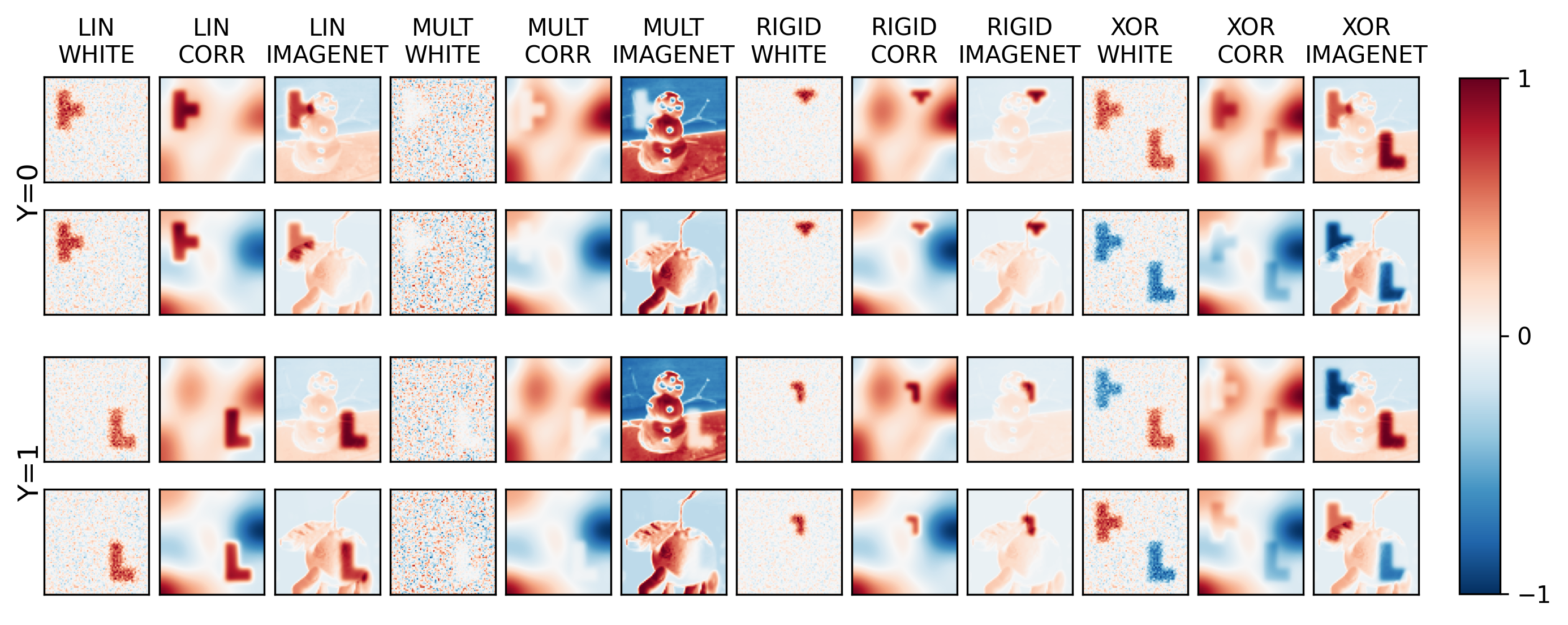
With each classification scenario defined, we can form the ground truth feature set of important pixels for a given input based on the positions of tetromino pixels as
| (3) |
For the LIN and MULT scenarios, each sample either contains a ‘T’ or an ‘L’ tetromino at a fixed position, corresponding to the fixed patterns and . Since the absence of a tetromino at one location is just as informative as the presence of the other at another location, we augment the set of important pixels for these two settings as
| (4) |
Note that this definition is equivalent to Eq. (3) for the XOR scenario. Moreover, it is equivalent to an operationalization of feature importance put forward by Wilming et al 2022 for the three static scenarios LIN, MULT, and XOR. Wilming et al 2022 define any feature as important if it has a statistical dependency to the prediction target across the studied sample. In all cases, an ideal explanation method should attribute importance only to members of the set .
For training each model and the subsequent analyses, we divide each dataset three-fold by a split into a training set , a validation set , and a test set .
2.2 Classifiers
We use three architectures to model each classification problem. Firstly, a Linear Logistic Regression (LLR) model, which is a single-layer neural network with two output neurons and a softmax activation function. Secondly, a Multi-Layer Perceptron (MLP) with four fully-connected layers, where each of the hidden layers uses Rectified Linear Unit (ReLU) activations. The two-neuron output layer is once again softmax-activated. Finally, we define a Convolutional Neural Network (CNN) with four blocks of ReLU-activated convolutional layers followed by a max-pooling operation, with a softmax-activated two-neuron output layer. The convolutional layers are specified with a progressively increasing amount of filters per layer , a kernel size of four, a stride of one, and zero-padding. The max-pooling layers are defined with a kernel size of two and a stride of one.
We train a given classifier over parameterization and . Each network is trained over 500 epochs using the Adam optimizer without regularization, with a learning rate of . The validation dataset is used at each step to get a sense of how well the model is generalizing the data. Validation loss is calculated at each epoch and used to judge when the classifier has reached optimal performance, by storing the model state with minimum validation loss. This also prevents using an overfit model. Finally, the test dataset is used to calculate the resulting model performance, and is used in the evaluation of XAI methods. We consider a classifier to have generalized the given classification problem when the resulting test accuracy is at or above a threshold of .
Each network is implemented in PyTorch, and also in Keras with a TensorFlow backend, so to experiment over a wider variety of XAI methods implemented using either the Captum (Kokhlikyan et al 2020) or iNNvestigate (Alber et al 2018) frameworks. The main text focuses on the former.
2.3 XAI methods and performance baselines
We compare sixteen popular XAI methods in our analysis. The main text focuses on the results of four: Local Interpretable Model Explanations (LIME) (Ribeiro et al 2016), Layer-wise Relevance Propagation (LRP) (Bach et al 2015), SHapley Additive exPlanations (SHAP) (Lundberg and Lee 2017) and Integrated Gradients (Sundararajan et al 2017).
The full list is detailed in Appendix 9.5. This briefly summarizes each method, and provides the details of which library was used for implementation, Captum (Kokhlikyan et al 2020) or iNNvestigate (Alber et al 2018), as well as the specific parameterization for each method. Generally, we follow the default parameterization for each method. Where necessary, we specify the baseline as the zero input , a common choice in the field (Mamalakis et al 2022).
The input to an XAI method is a model , trained according to parameterization over , the -th test sample to be explained , as well as the baseline reference point for relevant methods. The method produces an ‘explanation’ .
We include four model-ignorant methods to generate ‘baseline’ importance maps for comparison with the aforementioned XAI methods. Firstly, we consider the Sobel filter, which uses both a horizontal and a vertical filter kernel to approximate first-order derivatives of data. Secondly, we use the Laplace filter, which uses a single symmetrical kernel to approximate second-order derivatives of data. Both are edge detection operators, and are given for each test sample as an input. Thirdly, we use a sample from a random uniform distribution . Finally, we use the rectified test data sample itself as an importance map.
2.4 Explanation performance metrics
Based on the well-defined ground truth set of class-dependent features for a given sample , we can readily form quantitative metrics to evaluate the quality of an explanation.
Precision
Omitting the sample-dependence in the notation, we define precision as the fraction of the features of with the highest absolute-valued importance scores contained within the set itself, over the total number of important features in the sample. We constrain these results to the submitted appendices, and focus on the results and analyses for the next two defined metrics.
Earth mover’s distance (EMD)
The Earth mover’s distance (EMD), also known as the Wasserstein metric, measures the optimal cost required to transform one distribution to another. We can apply this to the cost required to transform a continuous-valued importance map into , where both are normalized to have the same mass. The Euclidean distance between pixels is used as the ground metric for calculating the EMD, with denoting the cost of the optimal transport from explanation to ground truth . This follows the algorithm proposed by Bonneel et al 2011 and the implementation of the Python Optimal Transport library (Flamary et al 2021). We define a normalized EMD performance score as
| (5) |
where is the maximum Euclidean distance between any two pixels.
Remark.
Note that the ground truth defines the set of important pixels based on the data generation process. It is conceivable, though, that a model uses only a subset of these for its prediction, which must be considered equally correct. The above explanation performance metrics do not fully achieve invariance in that respect. However, both are designed to de-emphasize the impact of false-negative omissions of features in the ground truth on performance, while emphasizing the impact of false-positive attributions of importance to pixels not contained in the ground truth.
2.5 Importance Mass Accuracy
Because of this, we consider a third metric, Importance Mass Accuracy (IMA). Calculated as the sum of importance attributed to the ground truth features over the total attribution in the image, this metric is akin to ‘Relevance mass accuracy’ as defined by Arras et al 2022. We calculate
| (6) |
This metric achieves invariance for not penalizing false negative attribution to a subset of pixels in , whilst also utilizing the whole attribution instead of a ‘top-k’ metric such as Precision. Not only this, but it is a direct measure of false positive attribution, where a score of signals a perfect explanation highlighting only ground truth features as important. We use this metric to complement the strengths of whilst also presenting an alternative perspective to quantifying explanation performance.
3 Experiments
Our experiments aim to answer four main questions:
1. Which XAI methods are best at identifying truly important features as defined by the sets ?
2. Does explanation performance for each method remain consistent when moving from explaining a linear classification problem to problems with different degrees of non-linearity?
3. Does adding correlations to the background noise, through smoothing with the Gaussian convolution filter, negatively impact explanation performance?
4. How does the choice of model architecture impact explanation performance?
We generate a dataset for each scenario across a range of 20 choices of , finding the ‘sweet spot’ where average test accuracy over 10 trained models is at or above 80%. Table 1 shows the resulting values as well as the average test accuracy for each scenario, over five model trainings for datasets of size of each scenario. For training each model and the subsequent analyses, we divide each dataset three-fold by an split into a training set , a validation set , and a test set . From this, we compute absolute-valued importance maps for the intersection of test data correctly predicted by every appropriate classifier. The full table of training results for finding appropriate SNRs can be seen in Appendix 9.5.
| WHITE | CORR | IMAGENET | |||||
|---|---|---|---|---|---|---|---|
| ACC | ACC | ACC | |||||
| LLR | |||||||
| LIN | MLP | ||||||
| CNN | |||||||
| MULT | MLP | ||||||
| CNN | |||||||
| RIGID | MLP | ||||||
| CNN | |||||||
| XOR | MLP | ||||||
| CNN | |||||||
Experiments were run on an internal CPU and GPU cluster, with total runtime in the order of a matter of hours.
4 Results

Figure 2 depicts examples of absolute-valued importance maps produced for a random correctly-predicted sample for each scenario and model. Shown are results for four XAI methods (Gradient SHAP, LIME, LRP, and PatternNet respectively) for each of the three models (LLR, MLP, CNN respectively) followed by the model-ignorant Laplace filter. Appendix 9.7.1 expands on the qualitative results of the main text, and Figure 7 shows the absolute-valued global importance heatmaps for the LIN, MULT, and XOR scenarios, given as the mean of all explanations for every correctly-predicted sample of the given scenario and XAI method. As the RIGID scenario has no static ground truth pattern, calculating a global importance map is not possible.


Figure 3 shows explanation performance of individual sample-based importance maps produced by the selected XAI and baseline methods, across five models trained for each scenario-architecture parameterization, in terms of the and metrics. Appendix 9.7.2 expands on the quantitative results of the main text, detailing results for all 16 methods studied and for our Precision metric. In a few cases, performance tends to decrease as model complexity increases (from the simple LLR to the complex CNN architecture). One notable exception is for the RIGID scenario, where the CNN outperforms other models as expected. However, in this setting nearly all XAI methods are outperformed by a simple Laplace edge detection filter for correlated backgrounds results. In this case, the discrepancy between the MLP and CNN performance is amplified for the metric, with the CNN performing relatively better for a few XAI methods. The CNN also performs well in the case of the more-complicated IMAGENET backgrounds.
Within most scenario-architecture parameterizations, the performances of the studied XAI methods are relatively homogeneous, with a few exceptions. In most cases, correlated backgrounds (CORR) lead to worse explanation performance than their white noise (WHITE) counterparts, suggesting that suppressors in the smoothed background are difficult to distinguish from the class-dependent variables for most XAI methods. This effect can be most strongly observed when comparing RIGID WHITE to RIGID CORR for the metric, suggesting that correlations in the background do indeed increase false positive attribution in model explanations.
Baseline methods tend to perform similarly to one another. Interestingly, their performance is on par or even superior to various XAI methods in certain scenarios. Most notably, a simple Laplace edge detection filter outperforms nearly all other methods in the RIGID as well as the XOR scenarios, when used in combination with correlated backgrounds (CORR). results for baseline methods in the RIGID scenario show a lot less variance in the boxplots of Figure 3(b) than for the equivalents in Figure 3(a).
The results for the RIGID scenarios may be taken with a pinch of salt, as the high signal-to-noise ratios (SNRs) lead to highly salient tetrominoes in sample images. Notably, explanations produced for CNNs in this case tend to perform very well for both the and metrics compared to most results for any other model architecture and problem scenario. While this problem itself (identifying a pattern with rotation and scaling invariance) is the most realistic of the four presented here, particularly when applied to CNNs, the high saliency of tetrominoes is perhaps not wholly akin to realistic problem settings, where the relative saliency of individual objects of interest is usually far lower. The high saliency of the tetrominoes derives from our experimental choice to adjust SNRs to achieve a predefined minimal classification performance threshold, which required high SNR in this setting. An alternative approach could be to reverse this and fix the SNR for all scenarios and background types.
To revisit the stated questions from the start of Section 3:
1. Which XAI methods are best at identifying truly important features as defined by the sets ?
The results show massive variability in performance for all methods across all problems and model architectures, so we cannot declare one specific ‘best’ method.
2. Does explanation performance for each method remain consistent when moving from explaining a linear classification problem to problems with different degrees of non-linearity?
Here we can see again that some methods vary in performance depending on the type of non-linearity (most perform better for MULT with the fixed position non-linearity than for RIGID), with a larger spread of and scores (seen in the size of boxes and whiskers of Figure 3) for non-linear scenarios than for LIN.
The results for PatternNet and PatternAttribution (Kindermans et al 2018) shown in the appendix (Figures 8, 9 10, 16, and 17) were proposed in part for solving the suppressor problem, and we can see how this is not necessarily always the case. These methods show strong performance for LIN as proposed, and as was seen in Wilming et al 2022, but do not look to generalize as well in most non-linear scenarios. Notably when the pattern signal is not in a fixed position (i.e., RIGID), these methods perform worse than when the signal is in a fixed position (i.e., MULT and XOR). More specifically, they also look to learn the complete pattern signal (i.e., the tetromino shapes for both classes), so in the XOR case where both shapes are present and fixed in each sample, they do outright perform the best as one might expect.
3. Does adding correlations to the background noise, through smoothing with the Gaussian convolution filter, negatively impact explanation performance?
When looking at results from WHITE to CORR, we can spot a decrease in performance and increase in spread in most cases. This can be attributed to the fact that the imposed correlations (induced through Gaussian smoothing) between background pixels correlated with those overlapping with cause background pixels to act as suppressor variables. One can control the strength of this effect by increasing/decreasing the strength of the Gaussian smoothing’s sigma parameter.
4. How does the choice of model architecture impact explanation performance?
For LIN, explanation performance of all methods for all architectures is similar in most cases. When moving to non-linear scenarios, we can see little consistency in how architectures perform - the CNN can be seen to perform best in the RIGID case, but the MLP performs relatively better for the fixed tetromino position cases of MULT and XOR. This can perhaps be explained by the CNN architecture tending itself well to rotation/translation invariance, whereas the properties of the MLP work better for a fixed-position ground-truth class-conditional distribution.
We can also note that when multiple models present similar classification performance for a task, a user may assume or just not realize that explanation performance could be vastly different, as seen in the MLP vs CNN results of RIGID in Figure 3, and qualitatively in Figure 2 across all architectures.
5 Discussion
Experimental results confirm our main hypothesis that explanation performance is lower in cases where the class-specific signal is combined with a highly auto-correlated class-agnostic background (CORR) compared to a white noise background (WHITE). The difficulty of XAI methods to correctly highlight the truly important features in this setting can be attributed to the emergence of suppressor variables. Importantly, the misleading attribution of importance by an XAI method can lead to misinterpretations regarding the functioning of the predictive model, which could have severe consequences in practice. Such consequences could be unjustified mistrust in the model’s decisions, unjustified conclusions regarding the features related to a certain outcome (e.g., in the context of medical diagnosis), and a reinforcement of such false beliefs in human-computer interaction loops.
We have also seen that when multiple ML architectures can be used interchangeably to appropriately solve a classification problem – here with classification accuracy required to be above 80% – they may still produce disparate explanations. Architectures not only differed with respect to the selection of pixels within the correct set of important features, but also showed different patterns of false positive attributions of importance to unimportant background features. If one cannot produce consistent and sensical results for multiple seemingly appropriate ML architectures, the risk of model mistrust may be especially pronounced.
A recent survey showed that one in three XAI papers evaluate methods exclusively with anecdotal evidence, and one in five with user studies (Nauta et al 2023). Other work in the field tends to focus on secondary criteria (such as stability and robustness (Rosenfeld et al 2021-03-27; Hedström et al 2022)) or subjective or potentially circular criteria (such as fidelity and faithfulness (Gevaert et al 2022; Nauta et al 2023)). It was recently shown in Wilming et al 2023 that faithfulness as a concept can be treated as an XAI method in itself, and when done so is also prone to the attribution of arbitrarily high importance to suppressor variables. We therefore doubt that such secondary validation approaches can fully replace metrics assessing objective notions of ‘correctness’ of explanations, considering that XAI methods are widely intended to be used as means of quality assurance for machine learning systems in critical applications. Thus, the development of specific formal problems to be addressed by XAI methods, and the theoretical and empirical validation of respective methods to address specific problems, is necessary. In practice, a stakeholder may often (explicitly or implicitly) expect that a given XAI method identifies features that are truly related to the prediction target. In contrast to other notions of faithfulness, this is an objectively quantifiable property of an XAI method, and we here propose various non-linear types of ground-truth data along with appropriate metrics to directly measure explanation performance according to this definition. While our work is not the first to provide quantitative XAI benchmarks (Tjoa and Guan 2020; Li et al 2021; Zhou et al 2022; Arras et al 2022; Gevaert et al 2022; Agarwal et al 2022, see,), our work differs from most published papers in that it allows users to quantitatively assess potential misinterpretations caused by the presence of suppressor variables in data.
One potential limitation of the metric is the strictness of limiting the ground truth feature set to the specific pixels of tetrominoes compared to, say, the set of features outlining . Alternative definitions of could be conceived to more flexibly adapt to different potential ‘explanation strategies’. Figure 6 in the appendices outlines four ‘explanation strategies’ and how the metric varies with each. Notably, an ‘outline’ explanation performs worse than an explanation highlighting a subset of . This highlights two interesting features of our novel metric. Firstly, a strongly performing ‘subset’ explanation shows that does not penalize false negatives (not attributing high importance to some truly important features) as harshly as Precision and other ‘top-k’ metrics do. Secondly, the ‘outline’ explanation functions in a presumably similar way to some model-ignorant edge detection methods, and performs the worst of any explanation strategy shown in Figure 6. Yet, we have shown such edge detection methods to be capable of outperforming many XAI methods in some problem scenarios. Our metric also complements this potential limitation of , where it does not matter if the attribution of importance to features of is spread across all features, or just more intensely attributed to a subset. This metric directly measures false positive attribution of importance to features outside of , and assists the user in understanding the role that suppressors play in model explanations.
While we compare a total of 16 XAI methods, the space of possible neural network architectures is too vast to be represented; therefore we only compared one MLP and one CNN architecture here. However, our experiments hopefully serve as a showcase for our benchmarking framework, which can be easily extended to other architectures. Finally, our framework serves much needed validation purposes for methods that are conceived to themselves play a role in the quality assurance of AI. As such, we expect that the benefits of our work far outweigh potential negative implications on society, if any. A possible risk, even if far-fetched, would be that one may reject a fit-for-purpose XAI method based on empirical benchmarks such as ours, which do not necessarily reflect the real-world setting and may hence be too strict.
6 Conclusion
We have used a data-driven generative definition of feature importance to create synthetic data with well-defined ground truth explanations, and have used these to provide an objective assessment of XAI methods when applied to various classification problems. Furthermore, we have defined new quantitative metrics of explanation performance and demonstrated that many popular XAI methods do not behave in an ideal way when moving from linear to non-linear scenarios. Our results show that XAI methods can even be outperformed by simple model-ignorant edge detection filters in the RIGID use case, in which the object of interest is not located in a static position. Finally, we show that XAI methods may provide inconsistent explanations when using different model architectures under equivalent conditions. Future work will be to develop dedicated performance benchmarks in more complex and application-specific problem settings such as medical imaging.
7 Declarations
Funding - This result is part of a project that has received funding from the European Research Council (ERC) under the European Union’s Horizon 2020 research and innovation programme (Grant agreement No. 758985), the German Federal Ministry for Economic Affairs and Climate Action (BMWK) within the “Metrology for Artificial Intelligence in Medicine (M4AIM)” program in the frame of the “QI-Digital” initiative, and the Heidenhain Foundation in the frame of the Junior Research Group “Machine Learning and Uncertainty”.
Conflicts of interest/Competing interests - The authors declare no conflicts of interest/competing interests.
Availability of data and material - All data used here can be generated using the provided code.
Code availability - https://github.com/braindatalab/xai-tris
Ethics approval - Not applicable.
Consent to participate - Not applicable.
Consent for publication - Not applicable.
Author contributions - All authors contributed to the study conception and design. Material preparation, data collection and analysis were performed by Benedict Clark. The first draft of the manuscript was written primarily by Benedict Clark, and all authors commented on and edited all previous versions of the manuscript. All authors read, edited, and approved the final manuscript.
References
- Agarwal et al (2022) Agarwal C, Krishna S, Saxena E, et al (2022) Openxai: Towards a transparent evaluation of model explanations. Advances in Neural Information Processing Systems 35:15784–15799
- Alber et al (2018) Alber M, Lapuschkin S, Seegerer P, et al (2018) iNNvestigate neural networks!, 1808.04260
- Arras et al (2022) Arras L, Osman A, Samek W (2022) Clevr-xai: A benchmark dataset for the ground truth evaluation of neural network explanations. Information Fusion 81:14–40
- Asano et al (2021) Asano YM, Rupprecht C, Zisserman A, et al (2021) Pass: An imagenet replacement for self-supervised pretraining without humans. NeurIPS Track on Datasets and Benchmarks
- Bach et al (2015) Bach S, Binder A, Montavon G, et al (2015) On pixel-wise explanations for non-linear classifier decisions by layer-wise relevance propagation. PLOS ONE 10(7):1–46
- Bonneel et al (2011) Bonneel N, Van De Panne M, Paris S, et al (2011) Displacement interpolation using lagrangian mass transport. In: Proceedings of the 2011 SIGGRAPH Asia conference, pp 1–12
- Castro et al (2009) Castro J, Gómez D, Tejada J (2009) Polynomial calculation of the shapley value based on sampling. Computers & Operations Research 36(5):1726–1730. Selected papers presented at the Tenth International Symposium on Locational Decisions (ISOLDE X)
- Conger (1974) Conger AJ (1974) A Revised Definition for Suppressor Variables: A Guide To Their Identification and Interpretation , A Revised Definition for Suppressor Variables: A Guide To Their Identification and Interpretation. Educational and Psychological Measurement 34(1):35–46
- Deng et al (2009) Deng J, Dong W, Socher R, et al (2009) Imagenet: A large-scale hierarchical image database. In: 2009 IEEE conference on computer vision and pattern recognition, Ieee, pp 248–255
- Fisher et al (2019) Fisher A, Rudin C, Dominici F (2019) All Models are Wrong, but Many are Useful: Learning a Variable’s Importance by Studying an Entire Class of Prediction Models Simultaneously. Journal of Machine Learning Research 20(177):1–81
- Flamary et al (2021) Flamary R, Courty N, Gramfort A, et al (2021) Pot: Python optimal transport. Journal of Machine Learning Research 22(78):1–8
- Friedman and Wall (2005) Friedman L, Wall M (2005) Graphical Views of Suppression and Multicollinearity in Multiple Linear Regression. The American Statistician 59(2):127–136
- Gevaert et al (2022) Gevaert A, Rousseau AJ, Becker T, et al (2022) Evaluating Feature Attribution Methods in the Image Domain. arXiv e-prints arXiv:2202.12270. arXiv:2202.12270 [cs.CV]
- Golomb (1996) Golomb SW (1996) Polyominoes: puzzles, patterns, problems, and packings, vol 111. Princeton University Press
- Haufe et al (2014) Haufe S, Meinecke F, Görgen K, et al (2014) On the interpretation of weight vectors of linear models in multivariate neuroimaging. NeuroImage 87:96–110
- Hedström et al (2022) Hedström A, Weber L, Bareeva D, et al (2022) Quantus: An explainable ai toolkit for responsible evaluation of neural network explanations. 10.48550/ARXIV.2202.06861, URL https://arxiv.org/abs/2202.06861
- Kindermans et al (2018) Kindermans PJ, Schütt KT, Alber M, et al (2018) Learning how to explain neural networks: Patternnet and patternattribution. In: International Conference on Learning Representations
- Kokhlikyan et al (2020) Kokhlikyan N, Miglani V, Martin M, et al (2020) Captum: A unified and generic model interpretability library for PyTorch, 2009.07896
- Li et al (2021) Li XH, Shi Y, Li H, et al (2021) An experimental study of quantitative evaluations on saliency methods. In: Proceedings of the 27th ACM sigkdd conference on knowledge discovery & data mining, pp 3200–3208
- Lundberg and Lee (2017) Lundberg SM, Lee SI (2017) A Unified Approach to Interpreting Model Predictions. In: Guyon I, Luxburg UV, Bengio S, et al (eds) Advances in Neural Information Processing Systems 30. Curran Associates, Inc., p 4765–4774
- Mamalakis et al (2022) Mamalakis A, Barnes EA, Ebert-Uphoff I (2022) Carefully choose the baseline: Lessons learned from applying xai attribution methods for regression tasks in geoscience
- Montavon et al (2017) Montavon G, Bach S, Binder A, et al (2017) Explaining NonLinear Classification Decisions with Deep Taylor Decomposition. Pattern Recognition 65:211–222
- Nauta et al (2023) Nauta M, Trienes J, Pathak S, et al (2023) From anecdotal evidence to quantitative evaluation methods: A systematic review on evaluating explainable ai. ACM Comput Surv 10.1145/3583558, URL https://doi.org/10.1145/3583558, just Accepted
- Prabhu and Birhane (2020) Prabhu VU, Birhane A (2020) Large image datasets: A pyrrhic win for computer vision? arXiv preprint arXiv:200616923
- Ribeiro et al (2016) Ribeiro MT, Singh S, Guestrin C (2016) " Why should I trust you?" Explaining the predictions of any classifier. In: Proceedings of the 22nd ACM SIGKDD International Conference on Knowledge Discovery and Data Mining, pp 1135–1144
- Rosenfeld et al (2021-03-27) Rosenfeld E, Ravikumar P, Risteski A (2021-03-27) The Risks of Invariant Risk Minimization, 2010.05761
- Selvaraju et al (2017) Selvaraju RR, Cogswell M, Das A, et al (2017) Grad-CAM: Visual Explanations from Deep Networks via Gradient-Based Localization. In: 2017 IEEE International Conference on Computer Vision (ICCV), pp 618–626
- Shrikumar et al (2017) Shrikumar A, Greenside P, Kundaje A (2017) Learning Important Features Through Propagating Activation Differences. ICML
- Simonyan et al (2014) Simonyan K, Vedaldi A, Zisserman A (2014) Deep inside convolutional networks: Visualising image classification models and saliency maps. In: Workshop at International Conference on Learning Representations
- Springenberg et al (2015) Springenberg J, Dosovitskiy A, Brox T, et al (2015) Striving for simplicity: The all convolutional net. In: ICLR (workshop track)
- Sundararajan et al (2017) Sundararajan M, Taly A, Yan Q (2017) Axiomatic Attribution for Deep Networks. In: ICML
- Tjoa and Guan (2020) Tjoa E, Guan C (2020) Quantifying Explainability of Saliency Methods in Deep Neural Networks, 2009.02899
- Wilming et al (2022) Wilming R, Budding C, Müller KR, et al (2022) Scrutinizing XAI using linear ground-truth data with suppressor variables. Machine Learning
- Wilming et al (2023) Wilming R, Kieslich L, Clark B, et al (2023) Theoretical behavior of XAI methods in the presence of suppressor variables. In: Krause A, Brunskill E, Cho K, et al (eds) Proceedings of the 40th International Conference on Machine Learning, Proceedings of Machine Learning Research, vol 202. PMLR, pp 37091–37107, URL https://proceedings.mlr.press/v202/wilming23a.html
- Zeiler and Fergus (2014) Zeiler MD, Fergus R (2014) Visualizing and Understanding Convolutional Networks. In: Fleet D, Pajdla T, Schiele B, et al (eds) Computer Vision – ECCV 2014. Springer International Publishing, Lecture Notes in Computer Science, pp 818–833
- Zhou et al (2022) Zhou Y, Booth S, Ribeiro MT, et al (2022) Do feature attribution methods correctly attribute features? In: Proceedings of the AAAI Conference on Artificial Intelligence, pp 9623–9633
8 MLJ Contribution Information Sheet
What is the main claim of the paper? Why is this an important contribution to the machine learning literature?
We claim that many post-hoc explanation methods consistently and reproducibly highlight certain input features that have no statistical dependency to the target variable predicted by the model. The existence of such so-called suppressor variables, and the false positive attribution of such variables as important, can lead to severe misinterpretations, which raises concerns regarding the correctness and utility of ‘explanations’ provided by explanation methods.
We create benchmark image datasets for one linear and three non-linear classification scenarios, in which the important class-conditional features are known by design. These scenarios are based on different types and combinations of tetrominoes (Golomb 1996), overlaid on one of three types of noisy backgrounds. One of these background types, white noise smoothed by a Gaussian filter, induces the presence of suppressor variables through the correlation of background pixels overlapping the tetromino with those just of the noisy background. In all cases, ground truth explanations are explicitly known through the location of the tetrominoes in the sample.
We develop novel performance metrics, one based on the Earth mover’s distance of transforming the ‘energy’ of a given explanation into the ground truth explanation, and use this to show that in many cases, the presence of induced suppressor variables hinders explanation performance for many popular XAI methods. Another metric directly measures the false positive attribution of model explanations through the proportion of importance attributed to ground truth features over the total attribution of the explanation. These two metrics complement each other well.
Through our experimental results we draw other conclusions, including that explanations produced for different equally performing ML architectures can be very inconsistent. We show that popular explanation methods are sometimes unable to outperform random performance baselines and edge detection methods. We highlight that secondary metrics such as faithfulness are currently not sufficient to assess ML explanation quality compared to objective metrics focused on the ‘correctness’ of explanations, such as those presented here.
The importance of these claims is that machine learning model explanations are prone to misinterpretation under such inconsistencies. For example, one may assume that equally performing models would produce equally performing explanations, however this is not always true. One may have chosen a particular architecture based on other properties of it, and end up with misleading or nonsensical explanations. We necessitate that for XAI to be deployed in high-stakes fields, such risks should be mitigated. Our approach is a rigorous and objective evaluation of the performance of current explanation methods, which can lead to the development of stronger and more reliable methods in the future.
What is the evidence you provide to support your claim? Be precise.
We conduct an extensive set of empirical experiments across 4 image classification problem scenarios, 3 background types, 3 model architectures, 16 explanation methods, 4 performance baselines, and 3 metrics. We carefully construct the important class-conditional features in each problem, which can serve as ground truth explanations. We assess many popular post-hoc XAI methods and quantify their ‘explanation performance’ using metrics from signal detection theory such as Earth mover’s distance, , and precision, and show that such methods attribute importance to suppressor variables and can lead to misleading interpretations.
Through our experimental results we observe behavior including that explanations produced for different equally performing ML architectures can be very inconsistent. We show that popular explanation methods are sometimes unable to outperform random performance baselines and edge detection methods for our developed performance metrics. We discuss, using related literature, that secondary metrics such as faithfulness are currently not sufficient to assess ML explanation quality compared to objective metrics focused on the ‘correctness’ of explanations, such as those presented here.
What papers by other authors make the most closely related contributions, and how is your paper related to them?
Several works in the XAI field have moved towards quantitative evaluation of XAI methods using ground truth data (Tjoa and Guan 2020; Li et al 2021; Zhou et al 2022; Arras et al 2022; Gevaert et al 2022; Agarwal et al 2022). However, these studies are limited in the extent to which they perform quantitative assessment, and many such studies do not construct their benchmark datasets in a way that realistic correlations between class-dependent and class-agnostic features (i.e., the foreground/object in an image vs. the background) are included. In practice, these correlations can give rise to features acting as suppressor variables. These works do not focus on such variables and our previous work is the only such work to do so.
Wilming et al 2022, published in ECML 2022, took a similar approach to that shown here, yet focused on a linear problem for one model architecture, and did not make use of random performance baselines to compare XAI methods to. Wilming et al 2023 also looked into quantifying explanation performance in the presence of suppressors using a two-dimensional linear example, however the focus there was on analytically deriving the exact influence of suppressors on produced explanations.
Have you published parts of your paper before, for instance in a conference? If so, give details of your previous paper(s) and a precise statement detailing how your paper provides a significant contribution beyond the previous paper(s).
The content of this paper is entirely original. Some ideas discussed in this paper have already been voiced in our prior work (Haufe et al 2014; Wilming et al 2022; Wilming et al 2023). However, our current paper goes beyond these through focusing on an extensive set of empirical experiments across 4 image classification problem scenarios, 3 background types, 3 model architectures, 16 explanation methods, 4 performance baselines, and 3 metrics.
Suggested Reviewers
Pieter-Jan Kindermans (pikinder@google.com): Author of PatternNet and PatternAttribution.
Moritz Grosse-Wentrup (moritz.grosse-wentrup@univie.ac.at): Expert in XAI and causality.
Max Welling (M.Welling@uva.nl): Esteemed machine learning expert with interest in XAI.
Robert Jenssen (robert.jenssen@uit.no): Professor of machine learning with track record in XAI.
9 Appendix
The authors confirm that we bear all responsibility in case of violation of rights of any kind in the data and results shown in this work.
9.1 ImageNet
We sample data from the ImageNet-1k subset (Deng et al 2009), following the license specified here https://image-net.org/download.php.
In the ImageNet-1k subset, there are only three people categories (scuba diver, bridegroom, and baseball player) included in the 1,000 classes, versus 2,832 people categories in the full set. There is also the possibility of people-related images co-existing in images of other classes, which has been noted (Prabhu and Birhane 2020). Data from these classes can be discarded if necessary.
Alternatives can be used directly as a background type here to replace ImageNet, for example PASS (Asano et al 2021), published in the NeurIPS Datasets and Benchmarks track in 2021. This ImageNet replacement dataset only contains images with a CC-BY license, as well as containing no images of humans. Replacement of ImageNet images in our work is as simple as placing images in the respective folder for the data generation step to handle, following the instructions outlined in the next sub-section and the corresponding GitHub repository.
9.2 Code and Data
All code for generating data and performing model training and XAI analysis is available on GitHub: https://github.com/braindatalab/xai-tris. There, we provide instructions on how to run each step of the analysis pipeline as well as detailing corresponding configuration fields.
To download the ImageNet data, we made an account and agreed the license terms on https://huggingface.co/datasets/imagenet-1k and subsequently downloaded the data. Here, we used the validation set as the set suited the volume requirement for our analysis. We of course advise anyone planning to do similar analysis on a model pre-trained with ImageNet data to use the test set instead.
Each dataset generated for a given classification scenario and background type pair is GB in size. For the lower-dimensional -px data and experiments shown in supplementary materials Section 9.8, generating datasets for all eight scenario and background type pairs is around MB in total size, and was combined in one file due to this much lower volume requirement. Each scenario’s dataset is saved as a file SCENARIO_JdKp__BACKGROUND.pkl containing a python dictionary
where SCENARIO={linear, multiplicative, translations_rotations, xor} and BACKGROUND={white, correlated, imagenet}. Image scale Jd={1,8}d is the scaling of the image dimensionality from the original -px images to the -px images shown in the main text, pattern scale Kp={1,4,8}p is the scaling of the tetromino pattern (width in pixels), and parameterizes the signal-to-noise ratio.
DataRecord is a Python namedtuple() collection specified as
Each field can be accessed programmatically via the name, for example DataRecord.x_test returns the test data of the dataset. The masks fields are the tetromino pattern masks which form the ground truth for explanations.
9.3 Compute
Experiments were run on a cluster consisting of four Nvidia A40 GPUs, where each model training took roughly between three and twenty minutes to complete, depending on architecture. Time estimation for running XAI methods is more rough to calculate and depends on each method, but in total for all models and methods for a given scenario’s test set, this took between 24 and 48 hours of compute time per GPU on the cluster. Quantitative analysis took roughly a further 24 hours of compute per scenario on a cluster of AMD EPYC 7702 CPUs, with six threads used for each of the 12 scenarios.
Due to smaller compute requirements, we can also recommend that if one wants to explore the code and data with smaller compute requirements, the -px data shown in supplementary materials Section 9.8 is also representative of a strong benchmark for XAI methods. Code and instructions to run it have also been provided in the GitHub repository linked in the above supplementary materials Section 9.2.
9.4 Data
Here, we expand on Figure 1 with Figure 4, which shows an example of each scenario across four choices of signal-to-noise ratio (SNR), parameterized by .

9.5 Explanation Methods and Model Training
Here, we detail the full suite of 16 XAI methods used in our analysis, with a brief description along with the reference and any parameterization details. In the main text, we focus on XAI methods available with the Captum (Kokhlikyan et al 2020) framework for explaining PyTorch models. We also make use of methods available in the iNNvestigate (Alber et al 2018) library, through training equivalent models for the Keras framework.
| XAI Method | Description | Implementation Framework, Parameterization | Reference |
| Permutation Feature Importance (PFI) | Measures the change in prediction error of the model after permuting each feature’s value | Captum, Default | Fisher et al 2019 |
| Integrated Gradients | Computes gradients along the path from a baseline input to the input sample, and cumulates these through integration to form an explanation | Captum, Default, Zero input baseline | Sundararajan et al 2017 |
| Saliency | Computes the gradients with respect to each input feature | Captum, Default | Simonyan et al 2014 |
| Guided Backpropagation | Computes the gradient of the output with respect to the input, but ensures only non-negative gradients of ReLU functions are backpropagated | Captum, Default | Springenberg et al 2015 |
| Guided GradCAM | Computes the element-wise product of guided backpropagation attributions with respect to a class-discriminative localization map in the final convolution layer of a CNN. This produces a coarse importance map for the target class as an explanation, the same size as the convolutional feature map, rather than pixel-wise over the whole image | Captum, Default | Selvaraju et al 2017 |
| Deconvolution | Uses a Deconvolutional network to map features to pixels. An explanation is produced by computing the gradient of the target output, only backpropagating non-negative gradients of ReLU functions | Captum, Default | Zeiler and Fergus 2014 |
| DeepLift | Compares the difference between the activation of each neuron and its ‘reference activation’, and produces an explanation based on this difference | Captum, Default, Zero input baseline | Shrikumar et al 2017 |
| Shapley Value Sampling | Approximates Shapley values by repeatedly sampling random permutations of input features and calculating the contribution of each feature to the prediction. An explanation is produced across an average of many samplings | Captum, Default, Zero input baseline | Castro et al 2009 |
| Gradient SHAP | Approximates Shapley values by computing the expected values of gradients when randomly sampled from the distribution of baseline samples | Captum, Default, Zero input baseline | Lundberg and Lee 2017 |
| Kernel SHAP | Approximates Shapley values through the use of LIME, setting the loss function, weighting kernel, and regularization term in accordance with the SHAP framework | Captum, Default, Zero input baseline | Lundberg and Lee 2017 |
| Deep SHAP | Approximates Shapley values through the use of DeepLift. Computes the DeepLift attribution for each input sample with respect to each baseline sample, in accordance with the SHAP framework | Captum, Default, Zero input baseline | Lundberg and Lee 2017 |
| Locally-interpretable Model Agnostic Explanations (LIME) | Learns a linear surrogate model locally to an individual prediction, perturbing and weighting the dataset in the process, and then builds an explanation by interpreting this local model | Captum, Default | Ribeiro et al 2016 |
| Layer-wise Relevance Propagation (LRP) | Propagates the model output back through the network as a measure of relevance, decomposing this score for each model in each layer based on their trained weight and activation | Captum, Default | Bach et al 2015 |
| Deep Taylor Decomposition (DTD) | Applies a Taylor decomposition from a specified root point to approximate the sub-functions of a network, building explanations by applying this backward from the network output to input variables | iNNvestigate, Default | Montavon et al 2017 |
| PatternNet | Estimates activation patterns per neuron through signal estimator and back-propagates this through the network. The explanation is given as a projection of the signal in input space | iNNvestigate, Default | Kindermans et al 2018 |
| PatternAttribution | Utilises the theory of PatternNet to estimate the root point of the data for DTD, and yields the attribution for weight vector and positive activation patterns . The explanation is given as the neuron-wise contribution of the signal to the classification score | iNNvestigate, Default | Kindermans et al 2018 |

9.6 Earth Mover’s Distance

9.7 Explanation Performance
This section further elaborates results of our experiments on validating the performance of XAI methods. In Figures 8 and 10 we also show methods available in the iNNvestigate (Alber et al 2018) library, through training equivalent models for the Keras framework. We note that there were some issues in convergence for CNN models for the XOR scenarios with the required Keras framework, even under seemingly equivalent conditions such as fixed random seeds and He-normal weight initialization. Our model architectures have been chosen as a showcase of the datasets and benchmarks of this work, and other architectures may have better or worse performance on the same XAI methods, but this was not a focus of this work. As such, we do not show the corresponding results for these methods (PatternNet, PatternAttribution, Deep Taylor Decomposition) in the XOR-CNN problem setting, so to promote a fair comparison of methods.
9.7.1 Qualitative Results
In Figure 7, we can see absolute-valued global importance maps for selected XAI methods and baselines, calculated as the mean importance value over all correctly predicted samples. RIGID scenarios involving translations and rotations of the tetromino signal pattern are not included as they have no fixed ground truth position.

9.7.2 Quantitative Results
In Figures 8, 9, and 10 we can see the full quantitative results for the , , and Precision metrics respectively, across all XAI methods and baselines. We can also see results for the PatternNet, PatternAttribution, and Deep Taylor Decomposition (DTD) methods, which are part of the Keras-based iNNvestigate framework (Alber et al 2018).


9.8 8x8 Benchmarks
The benchmark was originally designed around -px tetromino images, scaled up to -px with the inclusion of the ImageNet data as a third background type. This was done to improve the robustness and real-world applicability of the datasets and benchmarks present in this work. The original results for the -px data with -px thick tetrominoes can be seen in this section. Figure 11 shows example data for both classes and also across a range of four values. For CORR backgrounds, we set for the smoothing filter, and no pattern smoothing was incorporated. Here, each scenario was constructed with sample size and with an train/val/test split, with 25 datasets per scenario being used for analyses.
The Linear Logistic Regression (LLR) model in these experiments was the same single-layer neural network with two output neurons and a softmax activation function. The Multi-Layer Perceptron (MLP) similarly has four fully-connected layers and Rectified Linear Unit (ReLU) activations, and each of the fully-connected hidden layers halves the input size, i.e. [64, 32, 16, 8]. The two-neuron output layer was once again softmax-activated. Finally, the Convolutional Neural Network (CNN) was defined as four blocks of ReLU-activated convolutional layers followed by a max-pooling operation, with a softmax-activated two-neuron output layer. The convolutional layers are specified with four filters, a kernel size of two, a stride of one, and padding such that the input and output shapes match. This padding technique was used to improve pixel utilization across each convolution, as well as to mitigate shrinking outputs of the already relatively small images, by adding extra filler pixels (set to values of zero) around the edge of each image. The max-pooling layers are defined with a kernel size of two and a stride of two. As with the CNN architecture of the main text, some popular CNN architecture features (such as batch normalization) are unavailable here due to lack of implementation support by some XAI methods.
Figure 12 shows the training results across ten values along with Table 3 which shows the chosen values used for analysis. Each network was trained over 500 epochs using the Adam optimizer without regularization, with a learning rate of for the LIN, MULT, and XOR scenarios, and for the RIGID scenario.
Figures 13 and 14 show qualitative results for local and global explanations respectively, and Figures 16 and 17 show quantitative results for the and Precision metrics respectively.


| WHITE | CORR | ||||
|---|---|---|---|---|---|
| ACC | ACC | ||||
| LLR | |||||
| LIN | MLP | ||||
| CNN | |||||
| MULT | MLP | ||||
| CNN | |||||
| RIGID | MLP | ||||
| CNN | |||||
| XOR | MLP | ||||
| CNN | |||||


