跳到论文正文
W Papers独立论文阅读器 arXiv:2306.12569 论文正文 计算阅读时间 · 0%
引用这篇论文根据当前论文元数据生成,正式投稿前建议核对。


License: CC BY-NC-SA 4.0
arXiv:2306.12569v2 [quant-ph] 09 Feb 2024

Trotter error bounds and dynamic multi-product formulas for Hamiltonian simulationPreprint: APS/123-QED

Sergiy Zhuk Email: sergiy.zhuk@ie.ibm.com Affiliation: IBM Quantum, IBM Research Europe - Dublin, IBM Technology Campus, Dublin 15, Ireland    Sergey Bravyi Email: sbravyi@us.ibm.com Affiliation: IBM Quantum, IBM T.J. Watson Research Center    Niall F. Robertson Email: niall.robertson@ibm.com Affiliation: IBM Quantum, IBM Research Europe - Dublin, IBM Technology Campus, Dublin 15, Ireland
Abstract

Multi-product formulas (MPF) are linear combinations of Trotter circuits offering high-quality simulation of Hamiltonian time evolution with fewer Trotter steps. Here we report two contributions aimed at making multi-product formulas more viable for near-term quantum simulations. First, we extend the theory of Trotter error with commutator scaling developed by Childs, Su, Tran et al. to multi-product formulas. Our result implies that multi-product formulas can achieve a quadratic reduction of Trotter error in 1-norm (nuclear norm) on arbitrary time intervals compared with the regular product formulas without increasing the required circuit depth or qubit connectivity. The number of circuit repetitions grows only by a constant factor. Second, we introduce dynamic multi-product formulas with time-dependent coefficients chosen to minimize a certain efficiently computable proxy for the Trotter error. We use a minimax estimation method to make dynamic multi-product formulas robust to uncertainty from algorithmic errors, sampling and hardware noise. We call this method Minimax MPF and we provide a rigorous bound on its error.

I Introduction

Simulation of Hamiltonian dynamics is one of the most natural use cases for quantum computers. Such simulation can aid researchers in computing electronic structure of large molecules wang2008quantum; reiher2017elucidating, finding energy spectrum of elementary excitations harle2022observing, understanding thermalization in closed systems kaufman2016quantum, and testing theoretical models of a quantum chaos garttner2017measuring. It is strongly believed that Hamiltonian dynamics simulation is intractable for conventional classical computers due to an exponentially large dimension of the Hilbert space and highly entangled nature of time-evolved states. In contrast, quantum computers can efficiently simulate Hamiltonian dynamics for any spin or fermion system with few-body interactions lloyd1996universal or, more generally, for any sparse Hamiltonian low2017optimal.

Here we focus on a particular class of quantum simulation algorithms based on product formulas. A product formula is a quantum circuit 𝒮⁡(t){\cal S}(t) approximating the evolution operator e−i​t​He^{-itH} for a quantum system with a Hamiltonian HH evolved over time tt. The circuit 𝒮⁡(t){\cal S}(t) is usually chosen as a product of local evolution operators associated with few-body interactions describing the system. As such, product formulas inherit local structure of the underlying system which often obviates the need for long-range entangling gates. For example, simulating a spin chain Hamiltonian with short-range interactions would only require a hardware with the linear qubit connectivity. Furthermore, local structure of product formulas results in improved approximation error bounds that can exploit commutativity of non-overlapping Hamiltonian terms childs2021theory. Most of product formulas also exhibit a periodicity structure such that a few layers of gates simulating a short time step are repeated many times to simulate a longer evolution time. The periodicity structure aids error mitigation methods, such as the Probabilistic Error Cancellation temme2017error; berg2022probabilistic, as one has to learn noise models only for a few distinct layers of gates.

High-quality product formulas that accurately approximate Hamiltonian dynamics of practically relevant systems can be very deep. A common approach is to break the desired evolution time tt into kk intervals of length t/kt/k and apply a product formula kk times with the evolution time t/kt/k. This yields a circuit 𝒮​(t/k)k{\cal S}(t/k)^{k} whose depth scales linearly with kk. The required number of time steps kk depends on details of the Hamiltonian, desired approximation error, and the type of a product formula. For example, solving a benchmark simulation problem posed by Childs, Maslov, et al. childs2018toward for a system of 100100 qubits would require k≥5000k\geq 5000 time steps if one uses the fourth-order Trotter product formula, see Section F.3 of childs2018toward. The resulting circuit 𝒮​(t/k)k{\cal S}(t/k)^{k} would be too deep to execute reliably on near-term quantum processors lacking error correction.

Multi-product formulas introduced in the context of quantum computing by Childs and Wiebe childs2012hamiltonian and developed further in low2019well; vazquez2022well; rendon2022improved may provide a more viable path to near-term quantum simulations. The simplest example of a multi-product formula (MPF) is a linear combination ∑j=1rcj​𝒮​(t/kj)kj\sum_{j=1}^{r}c_{j}{\cal S}(t/k_{j})^{k_{j}}, where cjc_{j} are real or complex coefficients, 𝒮⁡(t){\cal S}(t) is some base product formula, and k1,…,krk_{1},\ldots,k_{r} is a sequence of integers. The jj-th term in the MPF approximates the desired evolution operator e−i​t​He^{-itH} by performing kjk_{j} steps of the base product formula with the evolution time t/kjt/k_{j}. The coefficients cjc_{j} can be chosen such that the errors introduced by each circuit 𝒮​(t/kj)kj{\cal S}(t/k_{j})^{k_{j}} approximately cancel each other enabling high-accuracy simulations with fewer time steps low2019well.

Refs. childs2012hamiltonian; low2019well envisioned implementing the whole MPF on a quantum computer using the linear combination of unitaries (LCU) method. This yields a simulation algorithm with a favorable asymptotic cost that scales nearly linearly with the evolution time and poly-logarithmically with the desired approximation error low2019well. However, this algorithm has not been experimentally demonstrated yet due to a high complexity of LCU circuits.

Here we adopt a simpler implementation of MPFs due to Vazquez, Egger, et al. vazquez2022well, Rendon, Watkins, and Wiebe rendon2022improved, see also endo2019mitigating. These authors realized that implementing the whole MPF on a quantum processor is not needed for certain tasks, such as computing time-evolved expected values of observables vazquez2022well or quantum phase estimation rendon2022improved. Instead, these tasks can be accomplished by implementing each individual circuit 𝒮​(t/kj)kj{\cal S}(t/k_{j})^{k_{j}} in the MPF on a quantum device and classical post-processing of the measured data. Such quantum-classical MPF can be described as a linear combination of density matrices μ⁡(t)=∑j=1rcj​ρkj​(t)\mu(t)=\sum_{j=1}^{r}c_{j}\rho_{k_{j}}(t), where ρk​(t)\rho_{k}(t) is a state obtained by applying kk steps of the base product formula to the initial state ρi​n\rho_{in} at time t=0t=0. Equivalently, ρk​(t)=𝒮​(t/k)k​ρi​n​𝒮​(t/k)−k\rho_{k}(t)={\cal S}(t/k)^{k}\rho_{in}{\cal S}(t/k)^{-k}. Assuming that μ⁡(t)\mu(t) is a good approximation of the exact time-evolved state ρ⁡(t)=e−i​t​H​ρi​n​ei​t​H\rho(t)=e^{-itH}\rho_{in}e^{itH}, the expected value of any observable Tr⁡(𝒪​ρ​(t))\mathrm{Tr}({\cal O}\rho(t)) can be approximated by a linear combination ∑j=1rcj​Tr​(𝒪​ρkj​(t))\sum_{j=1}^{r}c_{j}\mathrm{Tr}({\cal O}\rho_{k_{j}}(t)). The latter can be computed classically as long as a quantum processor provides an estimate of the expected values Tr⁡(𝒪​ρkj​(t))\mathrm{Tr}({\cal O}\rho_{k_{j}}(t)).

To reap the benefits of MPFs one needs to address two points. First, one needs to bound the approximation error ‖μ⁡(t)−ρ⁡(t)‖1\|\mu(t)-\rho(t)\|_{1}. To the best of our knowledge, such bounds were previously known only in the special case when the number of time steps kjk_{j} is sufficiently large so that e−itH/kj≈Ie^{-itH/k_{j}}\approx I for all jj, see  childs2012hamiltonian; rendon2022improved. Here we overcome this limitation by extending the theory of Trotter error with commutator scaling due to Childs, Su, Tran et al childs2021theory from regular product formulas to MPFs. We show that an MPF can achieve a quadratic reduction of the approximation error compared with the base product formula without increasing the requited circuit depth or required qubit connectivity, see Theorem 1 in Section III for a formal statement. To the best of our knowledge, this provides the first rigorous upper bound on the approximation error achieved by MPFs which holds for any evolution time tt and any number of time steps kjk_{j}. Numerical simulations suggest that the error scaling predicted by Theorem 1 is nearly tight, see Section V. Our main technical innovation is an integral representation of MPFs based on Euler–Maclaurin formula. It allows us to express the difference μ⁡(t)−ρ⁡(t)\mu(t)-\rho(t) in terms of nested commutators of the type studied in childs2021theory.

Secondly, one needs an efficient method for computing MPF coefficients cjc_{j}. Indeed, the best scenario would have been to find optimal coefficients minimizing the error ‖μ⁡(t)−ρ⁡(t)‖1\|\mu(t)-\rho(t)\|_{1} at any given time tt, which is equivalent to projecting ρ\rho onto MPF subspace, namely the subspace generated by ρk1​…​ρkr\rho_{k_{1}}\dots\rho_{k_{r}}. However, in practice this may not be possible since the exact solution ρ⁡(t)\rho(t) is unknown. Instead, a common strategy is the polynomial extrapolation method chin2010multi. It works by expanding ρkj​(t)\rho_{k_{j}}(t) in powers of 1/kj1/k_{j}. This gives Taylor series with the 00-th order term ρ⁡(t)\rho(t) corresponding to the limit kj→∞k_{j}\to\infty and higher order terms proportional to positive powers of 1/kj1/k_{j}. By choosing the coefficients cjc_{j} as a solution of a suitable linear system one can ensure that all unwanted lower-order terms in the above expansion cancel each other. This is the approach taken in childs2012hamiltonian; low2019well; vazquez2022well; rendon2022improved as well as in our upper bound on the MPF approximation error. However, the polynomial extrapolation method is sub-optimal as it forces the coefficients cjc_{j} to be time independent and ignores all structure of the simulated system.

Another important practical issue one needs to deal with while using MPF is that the coefficents of MPF formula are sensitive to the choice of kik_{i} as for certain kik_{i} the resulting Vandermonde matrix (17) is ill-conditioned numerically, hence the resulting vector of coefficients has large condition number ∑i|ci|\sum_{i}|c_{i}| and so cic_{i} might amplify sampling noise when computing the linear combination ∑i=1rci​Tr⁡(O​ρki​(t))\sum_{i=1}^{r}c_{i}\tr(O\rho_{k_{i}}(t)) provided Tr⁡(O​ρki​(t))\tr(O\rho_{k_{i}}(t)) is computed on a noisy quantum hardware. Restricting kik_{i} one may obtain so called well-conditioned MPFs vazquez2022well.

To overcome the aforementioned limitations we propose dynamic multi-product formulas. These are MPFs of the form μD​(t)=∑j=1rcj​(t)​ρkj​(t)\mu^{D}(t)=\sum_{j=1}^{r}c_{j}(t)\rho_{k_{j}}(t) with time-dependent coefficients cj​(t)c_{j}(t) chosen to minimize the error ‖μD​(t)−ρ⁡(t)‖F\|\mu^{D}(t)-\rho(t)\|_{F} measured in Frobenious norm. Dynamic MPF with optimal coefficients – let’s denote them by cFr​(t)c^{\mathrm{Fr}}(t), represents optimal projection of ρ⁡(t)\rho(t) onto MPF subspace w.r.t. Frobenious inner product. It will be demonstrated later (and in fact it is quite easy to see) that the optimal coefficients cFr​(t)c^{\mathrm{Fr}}(t) require computing overlaps between Trotter circuits such as Tr⁡(ρki​(t)​ρkj​(t))\mathrm{Tr}(\rho_{k_{i}}(t)\rho_{k_{j}}(t)) and also overlaps of ρ⁡(t)\rho(t) with circuits such as Tr⁡(ρ⁡(t)​ρkj​(t))\mathrm{Tr}(\rho(t)\rho_{k_{j}}(t)). The former can be efficiently estimated (with a small additive error) on a quantum computer (see Section IV for details). But overlaps such as Tr⁡(ρ⁡(t)​ρkj​(t))\mathrm{Tr}(\rho(t)\rho_{k_{j}}(t)) require extra considerations since ρ⁡(t)\rho(t) is not available. To approximate ρ⁡(t)\rho(t), let d​t>0dt>0 be a sufficiently small time step. Assume without the loss of generality that μD​(t−d​t)\mu^{D}(t-dt) is known and is a good proxy for ρ⁡(t−d​t)\rho(t-dt) (this is the case at least initially!). We approximate the unknown ρ⁡(t)\rho(t) by 𝒮​((d​t)/k0)k0​μD​(t−d​t)​𝒮​((d​t)/k0)−k0{\cal S}((dt)/k_{0})^{k_{0}}\mu^{D}(t-dt){\cal S}((dt)/k_{0})^{-k_{0}} for small d​t>0dt>0 and a natural k0k_{0}. Simple linear algebra allows us to formalize this process in the form of a linear discrete-time dynamical system which describes dynamics of the optimal projection coefficients cFr​(t)c^{\mathrm{Fr}}(t) over time. This system is subject to uncertainty: namely, the approximation error of ρ⁡(t)\rho(t) by μD​(t−d​t)\mu^{D}(t-dt), and the sampling error in estimating Tr⁡(ρki​(t)​ρkj​(t))\mathrm{Tr}(\rho_{k_{i}}(t)\rho_{k_{j}}(t)) on the device. To deal with this uncertainty we employ minimax estimation method zhuk2010minimax, an estimation technique designed to handle uncertainty in dynamical systems zhuk2021minimax; zhuk2023detectability, to find an estimate of the vector of optimal coefficients cFrc^{\mathrm{Fr}} in the presence of noise. We prove that this estimate is robust to uncertainty due to algorithmic errors and sampling noise. We refer to this technique as minimax MPF. A practically important advantage of minimax MPF over the static MPF is that the former can provide well-conditioned coefficients cic_{i} (i.e. ∑i|ci|\sum_{i}|c_{i}| is small) for any sequence of kik_{i} in contrast to the static MPF which is well-conditioned only for a restricted set of kik_{i}, and to find the latter set one needs to solve a combinatorial optimization problem (see Figure 1 below). The reason that minimax MPF provides well-conditioned coefficients is that the method involves a penalization term which is the product of the magnitude of the sampling error and the norm of the coefficients – this term simultaneously reduces the effect of sampling noise and the condition number of the coefficients. We show the effect of this penalization term in numerical simulations: minimax MPF outperforms the well-conditioned MPF and the best product formula.

Finally, we provide a rigorous upper bound on the estimation error of minimax MPF and demonstrate that it scales proportionally to the aforementioned upper-bound on MPF error. Last but not the least, minimax MPF requires solving small-scale convex optimization problems which can be solved efficiently.

The rest of this paper is organized as follows. We provide a necessary background on product formulas and the theory of Trotter error with commutator scaling in Section II, which is largely based on childs2021theory. Multi-product formulas and our bound on the Trotter errror (Theorem 1) are stated in Section III. We introduce minimax milti-product formulas in Section IV . The rigorous upper bound on the Trotter error is compared with numerical simulations in Section V. This section also reports numerical experiments with static, dynamic and minimax MPFs. Appendix A contains the proofs.

II Product formulas and Trotter error

Suppose HH is a Hamiltonian describing a quantum spin or fermionic system. Our goal is to simulate Hamiltonian dynamics governed by the the von Neumann equation

ρ˙​(t)=−i⁡[H,ρ⁡(t)],t≥0\dot{\rho}(t)=-i[H,\rho(t)],\qquad t\geq 0 (1)

with a fixed initial state ρ⁡(0)=ρi​n\rho(0)=\rho_{in}. Its solution is

ρ⁡(t)=e−i​t​H​ρi​n​ei​t​H.\rho(t)=e^{-itH}\rho_{in}e^{itH}. (2)

A common strategy for simulating Hamiltonian dynamics on a quantum computer relies on product formulas. Suppose we are given a decomposition

H=∑a=1dFa,H=\sum_{a=1}^{d}F_{a}, (3)

where FaF_{a} are hermitian operators such that each unitary e−i​t​Fae^{-itF_{a}} admits an efficient implementation by a quantum circuit for any evolution time tt. For example, this is the case if FaF_{a} is a sum of few-particle interactions that pairwise commute. A product formula associated with F1,…,FdF_{1},\ldots,F_{d} is an operator-valued function

𝒮(t)=e−i​t​Fd⋯e−i​t​F2e−i​t​F1.{\cal S}(t)=e^{-itF_{d}}\cdots e^{-itF_{2}}e^{-itF_{1}}. (4)

Condition Eq. (3) ensures that 𝒮⁡(t)=e−i​t​H+O⁡(t2){\cal S}(t)=e^{-itH}+O(t^{2}) in the limit t→0t\to 0. More generally, 𝒮⁡(t){\cal S}(t) is called an order-pp product formula if

𝒮⁡(t)=e−i​t​H+O⁡(tp+1){\cal S}(t)=e^{-itH}+O(t^{p+1}) (5)

in the limit t→0t\to 0. For example, suppose HH describes a chain of nn qubits with nearest-neighbor interactions, H=∑j=1n−1Hj,j+1H=\sum_{j=1}^{n-1}H_{j,j+1}. Then a second-order Trotter-type product formula can be chosen as

𝒮⁡(t)=e−i​t​F3​e−i​t​F2​e−i​t​F1{\cal S}(t)=e^{-itF_{3}}e^{-itF_{2}}e^{-itF_{1}} (6)

with F1=F3=(1/2)​(H1,2+H3,4+H5,6+…)F_{1}=F_{3}=(1/2)(H_{1,2}+H_{3,4}+H_{5,6}+\ldots) and F2=H2,3+H4,5+H6,7+…F_{2}=H_{2,3}+H_{4,5}+H_{6,7}+\ldots. In this example d=3d=3.

Given an integer k≥1k\geq 1 and a product formula 𝒮⁡(t){\cal S}(t), define a state ρk​(t)\rho_{k}(t) obtained from ρi​n\rho_{in} by applying kk steps of the product formula 𝒮⁡(t/k){\cal S}(t/k), that is,

ρk​(t)=𝒮​(t/k)k​ρi​n​𝒮​(t/k)−k.\rho_{k}(t)={\cal S}(t/k)^{k}\rho_{in}{\cal S}(t/k)^{-k}. (7)

We shall refer to the approximation error ‖ρk​(t)−ρ⁡(t)‖1\|\rho_{k}(t)-\rho(t)\|_{1} achieved by a product formula as a Trotter error. Recall that the 1-norm ‖X‖1\|X\|_{1} of an operator XX is defined as the sum of singular values of XX or, equivalently, as ‖X‖1=max𝒪⁡|Tr⁡(𝒪​X)|/‖𝒪‖\|X\|_{1}=\max_{\cal O}|\mathrm{Tr}({\cal O}X)|/\|{\cal O}\|, where the maximum is over all non-zero operators 𝒪{\cal O}. Using the standard properties of the 1-norm nielsen2002quantum and the triangle inequality one gets

‖ρk​(t)−ρ⁡(t)‖1\displaystyle\|\rho_{k}(t)-\rho(t)\|_{1} ≤2​‖𝒮​(t/k)k−e−i​t​H‖\displaystyle\leq 2\|{\cal S}(t/k)^{k}-e^{-itH}\|
≤2​k​‖𝒮⁡(t/k)−e−i⁡(t/k)​H‖.\displaystyle\leq 2k\|{\cal S}(t/k)-e^{-i(t/k)H}\|. (8)

A general upper bound on the error ‖𝒮⁡(t)−e−i​t​H‖\|{\cal S}(t)-e^{-itH}\| which is nearly tight in many cases of interest has been recently proved by Childs, Su, Tran, et al. childs2021theory. To state this bound we need some more notations. Suppose A1,…,As,BA_{1},\ldots,A_{s},B are linear operators acting on the same space. Define a quantity

αcomm​(p,A1,…,As,B)=∑q1,…,qs≥0q1+…+qs=pp!q1!⋯qs!\displaystyle\alpha_{\textbf{comm}}(p;A_{1},\ldots,A_{s};B)=\sum_{\begin{subarray}{c}q_{1},\ldots,q_{s}\geq 0\\ q_{1}+\ldots+q_{s}=p\\ \end{subarray}}\frac{p!}{q_{1}!\cdots q_{s}!}
⋅∥(AdA1)q1⋯(AdAs)qs(B)∥.\displaystyle\cdot\|(\mathrm{Ad}_{A_{1}})^{q_{1}}\cdots(\mathrm{Ad}_{A_{s}})^{q_{s}}(B)\|. (9)

Here AdX\mathrm{Ad}_{X} denotes the adjoint action of an operator XX, that is, AdX​(Y)=X​Y−Y​X\mathrm{Ad}_{X}(Y)=XY-YX for all operators YY. Assuming that the operators AA’s and BB have the units of energy, αcomm​(p,…)\alpha_{\textbf{comm}}(p;\ldots) has units [energy]p+1[\mathrm{energy}]^{p+1}. The following lemma is a corollary of the upper bound established in childs2021theory.

Lemma 1 (Trotter error).

Let ρ⁡(t)\rho(t) and ρk​(t)\rho_{k}(t) be the exact time evolved state and its approximation obtained by applying kk steps of an order-pp product formula, see Eqs. (2,7). Then for all t≥0t\geq 0

‖ρk​(t)−ρ⁡(t)‖1≤2​αp​tp+1(p+1)!​kp\|\rho_{k}(t)-\rho(t)\|_{1}\leq\frac{2\alpha_{p}t^{p+1}}{(p+1)!k^{p}} (10)

where

αp=∑a=2dαcomm​(p,Fd,…,Fa,Fa−1).\alpha_{p}=\sum_{a=2}^{d}\alpha_{\textbf{comm}}(p;F_{d},\ldots,F_{a};F_{a-1}). (11)

Since our setting is different from the one of Ref. childs2021theory, we provide a proof of Lemma 1 in Appendix A. As a concrete example, consider the second-order Trotter-type product formula Eq. (6). Then Eq. (11) gives

α2=|[F2,[F2,F1]]|+3​‖[F1,[F1,F2]]‖.\alpha_{2}=\|\,[F_{2},[F_{2},F_{1}]]\,\|+3\|\,[F_{1},[F_{1},F_{2}]]\,\|.

In general, αp\alpha_{p} involves the norm of order-pp nested commutators composed of F1,…,FdF_{1},\ldots,F_{d}. The quantity αp\alpha_{p} scales linearly with the system size nn for many interesting Hamiltonians such as quantum lattice models with short-range interactions childs2021theory. In this case the Trotter error Eq. (10) is proportional to n​tp+1/kpnt^{p+1}/k^{p} with a constant factor that depends on the order pp and details of the considered Hamiltonian.

III Multi Product Formulas

A multi product formula (MPF) approximates the exact time evolved state ρ⁡(t)\rho(t) by a linear combination

μ⁡(t)=∑i=1rci​ρki​(t)\mu(t)=\sum_{i=1}^{r}c_{i}\rho_{k_{i}}(t) (12)

where ρki​(t)\rho_{k_{i}}(t) is an approximation of ρ⁡(t)\rho(t) obtained by applying kik_{i} steps of some base product formula 𝒮⁡(t){\cal S}(t), see Eq. (7), and cic_{i} are real coefficients. All terms in μ⁡(t)\mu(t) use the same base product formula. The key idea behind MPFs is that errors introduced by each individual term in μ⁡(t)\mu(t) can be approximately cancelled with a proper choice of the coefficients cic_{i}. Thus the error ‖μ⁡(t)−ρ⁡(t)‖1\|\mu(t)-\rho(t)\|_{1} achieved by an MPF can be much smaller than the errors ‖ρki​(t)−ρ⁡(t)‖1\|\rho_{k_{i}}(t)-\rho(t)\|_{1} achieved by each term. We are interested in the error ‖μ⁡(t)−ρ⁡(t)‖1\|\mu(t)-\rho(t)\|_{1} minimized over the coefficients cic_{i}. Note that the optimal MPF μ⁡(t)\mu(t) might not be a physical state since some coefficients cic_{i} can be negative. Accordingly, one may not be able to prepare μ⁡(t)\mu(t) in the lab. However, this is not needed if one’s goal is just to compute an expected value of some observable 𝒪{\cal O} on ρ⁡(t)\rho(t). Indeed, suppose one can efficiently prepare each individual state ρki​(t)\rho_{k_{i}}(t) and obtain an estimate xi∈ℝx_{i}\in\mathbb{R} satisfying

|Tr⁡(𝒪​ρki​(t))−xi|≤ϵi\left|\mathrm{Tr}({\cal O}\rho_{k_{i}}(t))-x_{i}\right|\leq\epsilon_{i} (13)

for some error tolerance ϵi\epsilon_{i}. Assuming ‖𝒪‖≤1\|{\cal O}\|\leq 1 one gets

|Tr⁡(𝒪​ρ​(t))−∑i=1rci​xi|\displaystyle\left|\mathrm{Tr}({\cal O}\rho(t))-\sum_{i=1}^{r}c_{i}x_{i}\right| ≤‖μ⁡(t)−ρ⁡(t)‖1\displaystyle\leq\|\mu(t)-\rho(t)\|_{1}
+∑i=1rϵi|ci|.\displaystyle+\sum_{i=1}^{r}\epsilon_{i}|c_{i}|. (14)

The last term in Eq. (14) can be made arbitrarily small simply by improving the quality of estimates in Eq. (13). However, to avoid error amplification, the MPF must be well-conditioned low2019well such that the condition number κ=∑i=1r|ci|\kappa=\sum_{i=1}^{r}|c_{i}| is sufficiently small.

Let us first consider the error ‖μ⁡(t)−ρ⁡(t)‖1\|\mu(t)-\rho(t)\|_{1}. We stress that the existing rigorous error bounds for MPFs may not be applicable in the regime covered by Lemma 1. Indeed, assuming that the bound of Lemma 1 scales as O⁡(n​tp+1/kp)O(nt^{p+1}/k^{p}), where nn is the number of qubits, the base product formula needs only k=Ω⁡(n1/p​t1+1/p)k=\Omega(n^{1/p}t^{1+1/p}) time steps for an accurate simulation. Meanwhile, the existing error bounds for MPFs such as Lemma 10 of Ref. rendon2022improved are only applicable if minj⁡kj=Ω⁡(n​t)\min_{j}k_{j}=\Omega(nt), assuming that the Hamiltonian HH contains Ω⁡(n)\Omega(n) terms with the norm Ω⁡(1)\Omega(1). Applying such bounds to quantum advantage demonstrations in which tt is comparable or smaller than nn for a suitable choice of energy units childs2018toward; kim2023scalable would require each term in the MPF to perform at least Ω⁡(n2)\Omega(n^{2}) time steps, whereas Ω⁡(n1+2/p)\Omega(n^{1+2/p}) steps would suffice for the base product formula. Note that n1+2/p≪n2n^{1+2/p}\ll n^{2} for p≥3p\geq 3.

To justify the use of MPFs in the regime covered by Lemma 1, it is desirable to extend the theory of Trotter error with commutator scaling developed in childs2021theory from regular product formulas to MPFs. This is achieved in the following theorem. Our bound on the Trotter error depends on the norm of nested commutators analogous to αcomm\alpha_{\textbf{comm}} and αp\alpha_{p}, see Eqs. (II,11). Let us first define these commutators. Fix a product formula 𝒮(t)=e−i​t​Fd⋯e−i​t1​F1{\cal S}(t)=e^{-itF_{d}}\cdots e^{-it_{1}F_{1}} and consider a set of unitary operators

Γ(t)={e−i​τd​Fd⋯e−i​τ1​F1| 0≤τ1,…,τd≤t}.\Gamma(t)=\{e^{-i\tau_{d}F_{d}}\cdots e^{-i\tau_{1}F_{1}}\,|\,0\leq\tau_{1},\ldots,\tau_{d}\leq t\}.

Here we assume t≥0t\geq 0. Given a unitary U∈Γ⁡(t)U\in\Gamma(t), let U^\hat{U} be a linear map such that U^​(X)=U​X​U−1\hat{U}(X)=UXU^{-1} for any operator XX. Define a quantity

βcomm​(p,ℓ,A1,…,As,B,t)=∑q1,…,qs≥0q1+…+qs=pp!q1!⋯qs!\displaystyle\beta_{\textbf{comm}}(p,\ell;A_{1},\ldots,A_{s};B;t)=\sum_{\begin{subarray}{c}q_{1},\ldots,q_{s}\geq 0\\ q_{1}+\ldots+q_{s}=p\\ \end{subarray}}\frac{p!}{q_{1}!\cdots q_{s}!}
maxU∈Γ⁡(t)⋅∥(AdH)ℓU^(AdA1)q1⋯(AdAs)qs(B)∥.\displaystyle\max_{U\in\Gamma(t)}\cdot\|(\mathrm{Ad}_{H})^{\ell}\hat{U}(\mathrm{Ad}_{A_{1}})^{q_{1}}\cdots(\mathrm{Ad}_{A_{s}})^{q_{s}}(B)\|. (15)

Assuming that all operators AA’s and BB have the units of energy, βcomm​(p,ℓ,…)\beta_{\textbf{comm}}(p,\ell;\ldots) has units [energy]p+ℓ+1[\mathrm{energy}]^{p+\ell+1}. Let

βp,ℓ​(t)=∑a=2dβcomm​(p,ℓ,Fd,…,Fa,Fa−1,t).\beta_{p,\ell}(t)=\sum_{a=2}^{d}\beta_{\textbf{comm}}(p,\ell;F_{d},\ldots,F_{a};F_{a-1};t). (16)

Our main result is as follows.

Theorem 1 (MPF Trotter error).

Let ρ⁡(t)\rho(t) and ρk​(t)\rho_{k}(t) be the exact time evolved state and its approximation obtained by applying kk steps of an order-pp product formula. Consider a multi product formula μ⁡(t)=∑i=1rci​ρki​(t)\mu(t)=\sum_{i=1}^{r}c_{i}\rho_{k_{i}}(t) with r=p+1r=p+1. Suppose the coefficients cic_{i} solve a linear system

∑i=1rci=1and∑i=1rcikiq=0\sum_{i=1}^{r}c_{i}=1\quad\mbox{and}\quad\sum_{i=1}^{r}\frac{c_{i}}{k_{i}^{q}}=0 (17)

for q∈{p,p+1,…,2​p−1}q\in\{p,p+1,\ldots,2p-1\}. Then for all t≥0t\geq 0

‖μ⁡(t)−ρ⁡(t)‖1≤(∑i=1r|ci|ki2​p)​(a1​t2​p+2+a2​t2​p+1+a3​t2​p),\|\mu(t)-\rho(t)\|_{1}\leq\left(\sum_{i=1}^{r}\frac{|c_{i}|}{k_{i}^{2p}}\right)(a_{1}t^{2p+2}+a_{2}t^{2p+1}+a_{3}t^{2p}),

where

a1=8​(αp(p+1)!)2,a_{1}=8\left(\frac{\alpha_{p}}{(p+1)!}\right)^{2},
a2=4​β2​p,0​(0)(2​p)!+8​βp,p​(t/km​i​n)(2​π)p​p!,a_{2}=\frac{4\beta_{2p,0}(0)}{(2p)!}+\frac{8\beta_{p,p}(t/k_{min})}{(2\pi)^{p}p!},

and

a3=4​∑ℓ=1pBℓ​β2​p−ℓ,ℓ−1​(t/km​i​n)ℓ!​(2​p−ℓ)!.a_{3}=4\sum_{\ell=1}^{p}\frac{B_{\ell}\beta_{2p-\ell,\ell-1}(t/k_{min})}{\ell!(2p-\ell)!}.

Here BℓB_{\ell} is the ℓ\ell-th Bernoulli number and km​i​n=min⁡(k1,…,kr)k_{min}=\min{(k_{1},\ldots,k_{r})}.

Figure 1: Examples of multi-product formulas (MPFs) of order p=2,4,6p=2,4,6. Such MPFs have a form μ⁡(t)=∑i=1p+1ci​ρki​(t)\mu(t)=\sum_{i=1}^{p+1}c_{i}\rho_{k_{i}}(t) where ρki​(t)\rho_{k_{i}}(t) is an approximation of the exact time evolved state obtained by applying kik_{i} steps of the base product formula 𝒮⁡(t/ki){\cal S}(t/k_{i}). The sequence of time steps (k1,…,kp+1)(k_{1},\ldots,k_{p+1}) reported in the table was obtained by minimizing the factor ∑i=1p+1|ci|/ki2​p\sum_{i=1}^{p+1}|c_{i}|/k_{i}^{2p} in the upper bound of Theorem 1 over all tuples (k1,…,kp+1)(k_{1},\ldots,k_{p+1}) with 1≤ki≤km​a​x1\leq k_{i}\leq k_{max} and solving the linear system Eq. (17) with r=p+1r=p+1 to obtain the coefficients cic_{i}. To avoid clutter, we round the condition number and coefficients in the error scaling to the nearest integer. Note that the MPF approximation error can be reduced by performing a rescaling ki←λ​kik_{i}\leftarrow\lambda k_{i} for all ii, where λ≥1\lambda\geq 1 is any integer. The reduces the upper bound of Theorem 1 by the factor 1/λ2​p1/\lambda^{2p} without changing the coefficients cic_{i} and the condition number. Meanwhile, for the regular order-pp product formula, the rescaling k←λ​kk\leftarrow\lambda k reduces the approximation error only by the factor 1/λp1/\lambda^{p}, see Lemma 1.

In the limit of large evolution time tt the upper bound of Theorem 1 becomes

‖μ⁡(t)−ρ⁡(t)‖1≤(∑i=1r|ci|ki2​p)​a1​t2​p+2​[1+O⁡(1/t)].\|\mu(t)-\rho(t)\|_{1}\leq\left(\sum_{i=1}^{r}\frac{|c_{i}|}{k_{i}^{2p}}\right)a_{1}t^{2p+2}\left[1+O(1/t)\right]. (18)

Comparing this and Eq. (10) one infers that the MPF achieves a nearly quadratic reduction of error compared with the base product formula for large tt. To quantify this, we need to choose an explicit sequence (k1,…,kr)(k_{1},\ldots,k_{r}) and solve the linear system Eq. (17) to obtain the coefficients cic_{i}. Figure 1 shows examples of MPFs based on product formulas of order p=2,4,6p=2,4,6 with r=p+1r=p+1 terms and the maximum number of time steps per circuit km​a​x=25k_{max}=25. A sequence of time steps (k1,…,kr)(k_{1},\ldots,k_{r}) was selected by minimizing the sum ∑i=1r|ci|/ki2​p\sum_{i=1}^{r}|c_{i}|/k_{i}^{2p} over all rr-tuples (k1,…,kr)(k_{1},\ldots,k_{r}) with 1≤ki≤km​a​x1\leq k_{i}\leq k_{max}. Each of these examples can be turned to a family of MPFs by a rescaling ki←λ​kik_{i}\leftarrow\lambda k_{i}, where λ≥1\lambda\geq 1 is any integer. This reduces the MPF error by the factor 1/λ2​p1/\lambda^{2p} without changing the coefficients cic_{i} and the condition number κ\kappa (since the latter depend only on the ratios ki/kjk_{i}/k_{j}). In contrast, applying the rescaling k←λ​kk\leftarrow\lambda k to the base product formula reduces the approximation error only by the factor 1/λp1/\lambda^{p}, see Lemma 1. Thus MPFs with a constant condition number κ=O⁡(1)\kappa=O(1) achieve a quadratic error reduction compared with the base product formula without increasing the maximum number of time steps per circuit (and thus without increasing the circuit depth). The number of circuit repetitions grows only by a constant factor since the condition number amplifies the approximation error in Eq. (14).

The scaling of coefficients a2a_{2} and a3a_{3} in Theorem 1 with the number of qubits nn may depend on details of the Hamiltonian HH and the base product formula. In Appendix B we show that a2a_{2} and a3a_{3} scale at most linearly with nn for a large class of quantum spin Hamiltonians. This class includes any quantum lattice model with short-range bounded-norm interactions. However, we have to assume that the order pp and the number of exponents dd in the product formula are constants independent of nn.

We defer the proof of Theorem 1 to Appendix A. The proof relies on the machinery introduced in Ref. childs2021theory. Our main innovation is an integral representation of MPFs based on Euler–Maclaurin summation formula. Informally, this integral representation reduces the problem of bounding the MPF error to a single time step such that the error operator ρkj​(t)−ρ​(t)\rho_{k_{j}}(t)-\rho(t) can be viewed as a function of the variable t/kjt/k_{j} only. We consider Taylor series for this function at the point t/kj=0t/k_{j}=0. Terms of order less than 2​p2p in the Taylor series give a zero contribution to μ⁡(t)\mu(t) due to Eq. (17) and the assumption that the base product formula has order pp. The norm of the remaining terms of order at least 2​p2p can be bounded by the quantities proportional to (αp)2(\alpha_{p})^{2} or βp1,p2\beta_{p_{1},p_{2}} using Theorem 5 of Ref. childs2021theory. This theorem bounds the norm of truncated Taylor series for operator-valued functions such as e−i​t​AdFd⋯e−i​t​AdFa(Fa−1)e^{-it\mathrm{Ad}_{F_{d}}}\cdots e^{-it\mathrm{Ad}_{F_{a}}}(F_{a-1}). Unfortunately, this theorem does not apply to our problem out of the box because Euler–Maclaurin formula generates several unwanted terms proportional to derivatives of the considered function. To show that these derivative terms are sufficiently small, we generalize Theorem 5 of Ref. childs2021theory, as stated in Lemma 3 in Appendix A.

We expect that the upper bound of Theorem 1 can be strengthened to give a better than quadratic error suppression in the case r>p+1r>p+1 and leave this extension for a future work.

IV Minimax Multi-Product Formulas

In what follows we refer to MPF formula μS​(t)=∑i=1rci​ρki​(t)\mu^{S}(t)=\sum_{i=1}^{r}c_{i}\rho_{k_{i}}(t) with static cic_{i} and ρki​(t)\rho_{k_{i}}(t) defined as in the previous section as static MPF. By design, μS​(t)\mu^{S}(t) reduces the Trotter error compared with the regular product formulas but this error is not minimized, i.e. μS​(t)\mu^{S}(t) does not represent the optimal projection of ρ⁡(t)\rho(t) onto MPF subspace, namely the subspace generated by product formulas ρki​(t)\rho_{k_{i}}(t), i=1​…​ri=1\dots r. Noting that ‖ρ−μS‖F≤‖ρ−μS‖1≤r+1​‖ρ−μS‖F\|\rho-\mu^{S}\|_{F}\leq\|\rho-\mu^{S}\|_{1}\leq\sqrt{r+1}\|\rho-\mu^{S}\|_{F} in what follows we focus on minimizing the following projection error:

‖ρ⁡(t)−μD​(t)‖F2=Tr⁡((ρ⁡(t)−μD​(t))2)\|\rho(t)-\mu^{D}(t)\|_{F}^{2}=\mathrm{Tr}\left((\rho(t)-\mu^{D}(t))^{2}\right) (19)

over coefficients cic_{i} for each time tt. In other words, μD​(t)=∑i=1rciFr​(t)​ρki​(t)\mu^{D}(t)=\sum_{i=1}^{r}c^{\mathrm{Fr}}_{i}(t)\rho_{k_{i}}(t) is the optimal projection of ρ\rho onto MPF subspace in Frobenious norm. In what follows we refer to μD\mu^{D} as a dynamic MPF. A simple algebra gives

‖ρ⁡(t)−μD​(t)‖F2\displaystyle\|\rho(t)-\mu^{D}(t)\|_{F}^{2} =1+∑i,j=1rMi,j​(t)​ci​(t)​cj​(t)\displaystyle=1+\sum_{i,j=1}^{r}M_{i,j}(t)c_{i}(t)c_{j}(t)
−2∑i=1rLi𝖾𝗑𝖺𝖼𝗍(t)ci(t)\displaystyle-2\sum_{i=1}^{r}L_{i}^{\mathsf{exact}}(t)c_{i}(t) (20)

where M⁡(t)M(t) is the Gram matrix

Mi,j​(t)\displaystyle M_{i,j}(t) =Tr⁡(ρki​(t)​ρkj​(t))\displaystyle=\mathrm{Tr}(\rho_{k_{i}}(t)\rho_{k_{j}}(t))
=|⟨ψi​n|𝒮​(t/ki)−ki​𝒮​(t/kj)kj|ψi​n⟩|2\displaystyle=\left|\langle\psi_{in}|{\cal S}(t/k_{i})^{-k_{i}}{\cal S}(t/k_{j})^{k_{j}}|\psi_{in}\rangle\right|^{2} (21)

and L𝖾𝗑𝖺𝖼𝗍​(t)L^{\mathsf{exact}}(t) is a vector of overlaps

Li𝖾𝗑𝖺𝖼𝗍​(t)=Tr⁡(ρ⁡(t)​ρki​(t)).L_{i}^{\mathsf{exact}}(t)=\mathrm{Tr}(\rho(t)\rho_{k_{i}}(t)). (22)

If we knew both M⁡(t)M(t) and L𝖾𝗑𝖺𝖼𝗍​(t)L^{\mathsf{exact}}(t) then finding cFrc^{\mathrm{Fr}} by minimizing the right-hand side of Eq. (IV) over the coefficients c⁡(t)c(t) is straightforward. However, even though the Gram matrix M⁡(t)M(t) can be efficiently measured on hardware (with a small additive error), the vector of overlaps L𝖾𝗑𝖺𝖼𝗍​(t)L^{\mathsf{exact}}(t) is unknown since it depends on the the exact solution ρ⁡(t)\rho(t). To overcome this we approximate Li𝖾𝗑𝖺𝖼𝗍L_{i}^{\mathsf{exact}} and focus on estimating cFrc^{\mathrm{Fr}} by taking the approximation error into account.

Algorithmic error.

Assume that we need to approximate ρ⁡(t)\rho(t) on a segment [t0,T][t_{0},T]. Fix time step d​t>0dt>0 and select a uniform grid on [t0,T][t_{0},T]: tj=t0+j​d​tt_{j}=t_{0}+j\,dt, with integer j=0,…,(T−t0)/d​tj=0,\dots,(T-t_{0})/dt. We approximate ρ⁡(tj+1)\rho(t_{j+1}) by

ρ𝖺𝗉𝗉𝗋𝗈𝗑​(tj+1)=𝒮​(d​t/k0)k0​μD​(tj)​𝒮​(d​t/k0)−k0\rho^{\mathsf{approx}}(t_{j+1})={\cal S}(dt/k_{0})^{k_{0}}\mu^{D}(t_{j}){\cal S}(dt/k_{0})^{-k_{0}}

for an integer k0>0k_{0}>0. Then Li𝖾𝗑𝖺𝖼𝗍​(tj+1)L^{\mathsf{exact}}_{i}(t_{j+1}) is approximated by

Li𝖺𝗉𝗉𝗋𝗈𝗑​(tj+1)=Tr⁡(ρ𝖺𝗉𝗉𝗋𝗈𝗑​(tj+1)​ρki​(tj+1)).L_{i}^{\mathsf{approx}}(t_{j+1})=\tr\left(\rho^{\mathsf{approx}}(t_{j+1})\rho_{k_{i}}(t_{j+1})\right). (23)

and by linearity of the trace,

Li𝖺𝗉𝗉𝗋𝗈𝗑​(tj+1)=∑s=1rQi,s​(tj+1)​csFr​(tj),L_{i}^{\mathsf{approx}}(t_{j+1})=\sum_{s=1}^{r}Q_{i,s}(t_{j+1})c^{\mathrm{Fr}}_{s}(t_{j}), (24)

where

Qi,s\displaystyle Q_{i,s} (tj+1)=Tr⁡(𝒮​(d​tk0)k0​ρks​(tj)​𝒮​(d​tk0)−k0​ρki​(tj+1))\displaystyle(t_{j+1})=\tr\left({\cal S}(\frac{dt}{k_{0}})^{k_{0}}\rho_{k_{s}}(t_{j}){\cal S}(\frac{dt}{k_{0}})^{-k_{0}}\rho_{k_{i}}(t_{j+1})\right)
=|⟨ψi​n|𝒮​(tjks)−ks​𝒮​(d​tk0)−k0​𝒮​(tj+1ki)ki|ψi​n⟩|2\displaystyle=\left|\langle\psi_{in}|{\cal S}(\frac{t_{j}}{k_{s}})^{-k_{s}}{\cal S}(\frac{dt}{k_{0}})^{-k_{0}}{\cal S}(\frac{t_{j+1}}{k_{i}})^{k_{i}}|\psi_{in}\rangle\right|^{2} (25)

is a matrix that we can efficiently compute on hardware (with a small additive error). Making use of the above approximation we find that cFr​(tj)c^{\mathrm{Fr}}(t_{j}) solves: M⁡(tj)​cFr​(tj)=Q⁡(tj)​cFr​(tj−1)+L𝖾𝗑𝖺𝖼𝗍​(tj)−L𝖺𝗉𝗉𝗋𝗈𝗑​(tj)M(t_{j})c^{\mathrm{Fr}}(t_{j})=Q(t_{j})c^{\mathrm{Fr}}(t_{j-1})+L^{\mathsf{exact}}(t_{j})-L^{\mathsf{approx}}(t_{j}). To enforce Tr⁡(ρ𝖺𝗉𝗉𝗋𝗈𝗑​(t))=1\tr(\rho^{\mathsf{approx}}(t))=1 we require an extra constraint: 𝟙⊤​cFr​(t)=1\mathbb{1}^{\top}c^{\mathrm{Fr}}(t)=1 where 𝟙\mathbb{1} is the rr-dimensional vector of ones.

Shot noise.

In what follows we assume that the ”exact” matrices M⁡(t)M(t) and Q⁡(t)Q(t), defined by sections IV and IV respectively, belong to an ellipsoid centered around the given matrices M¯​(t)\bar{M}(t) and A¯​(t)\bar{A}(t):

M⁡(t)\displaystyle M(t) =M¯​(t)+E​(t)1⋆,Q⁡(t)=A¯​(t)+E​(t)2⋆\displaystyle=\bar{M}(t)+E(t)^{\star}_{1},\quad Q(t)=\bar{A}(t)+E(t)^{\star}_{2} (26)

with

‖E​(t)1,2⋆‖2,2≤ε\|E(t)^{\star}_{1,2}\|_{2,2}\leq\varepsilon (27)

for some unknown E1,2⋆​(t)E^{\star}_{1,2}(t) modelling hardware noise of the given magnitude ε\varepsilon in terms of ‖E⁡(t)‖2,2=max‖x‖2=1⁡‖E⁡(t)​x‖2\|E(t)\|_{2,2}=\max_{\|x\|_{2}=1}\|E(t)x\|_{2}. In other words: M⁡(t)∈{M¯​(t)+E1D​(t),‖E1D​(t)‖2,2≤ε}M(t)\in\{\bar{M}(t)+E^{D}_{1}(t),\|E^{D}_{1}(t)\|_{2,2}\leq\varepsilon\} and Q⁡(t)∈{A¯​(t)+E2D​(t),‖E2D​(t)‖2,2≤ε}Q(t)\in\{\bar{A}(t)+E^{D}_{2}(t),\|E^{D}_{2}(t)\|_{2,2}\leq\varepsilon\}. This assumption implies that cFrc^{\mathrm{Fr}} in fact solves:

(M¯​(tj)CLOSE\displaystyle(\bar{M}(t_{j}) OPEN+E1⋆​(tj))​cFr​(tj)=(A¯​(tj)+E2⋆​(tj))​cFr​(tj−1)\displaystyle+E^{\star}_{1}(t_{j}))c^{\mathrm{Fr}}(t_{j})=(\bar{A}(t_{j})+E^{\star}_{2}(t_{j}))c^{\mathrm{Fr}}(t_{j-1}) (28)
+L𝖾𝗑𝖺𝖼𝗍​(tj)−L𝖺𝗉𝗉𝗋𝗈𝗑​(tj),𝟙⊤​cFr​(t)=1.\displaystyle+L^{\mathsf{exact}}(t_{j})-L^{\mathsf{approx}}(t_{j}),\mathbb{1}^{\top}c^{\mathrm{Fr}}(t)=1\,. (29)

for unknown bounded matrices E1,2⋆​(t)E^{\star}_{1,2}(t) changing over time.

Minimax MPF.

In order to estimate cFr​(t)c^{\mathrm{Fr}}(t) we need means to estimate solution of eq. 28 which accounts for the error of approximating Li𝖾𝗑𝖺𝖼𝗍L_{i}^{\mathsf{exact}} by Li𝖺𝗉𝗉𝗋𝗈𝗑L^{\mathsf{approx}}_{i} and the measurement error (26). To this end we introduce the minimax MPF algorithm. The key difference to the dynamic MPF algorithm described above is the inclusion of a penalization term ε​‖x‖2\varepsilon\|x\|_{2} - see Algorithm 1 below.

input : window [t0,T][t_{0},T], cFr​(t0)c^{\mathrm{Fr}}(t_{0}), time step d​t>0dt>0, noise magnitude ε\varepsilon, and matrices M¯​(tj)\bar{M}(t_{j}), A¯​(tj)\bar{A}(t_{j}) for tj=t0+j​d​tt_{j}=t_{0}+jdt, j=0,…,(T−t0)/d​tj=0,\dots,(T-t_{0})/dt (see eq. 26)
output : estimate c^​(tj)\hat{c}(t_{j}) of cFr​(tj)c^{\mathrm{Fr}}(t_{j})
begin
Set c^​(t0)=cFr​(t0)\hat{c}(t_{0})=c^{\mathrm{Fr}}(t_{0});
    for j=1j=1 to (T−t0)/d​t(T-t_{0})/dt do
    tj:=t0+j​d​tt_{j}:=t_{0}+jdt, c^​(tj):=x^\hat{c}(t_{j}):=\hat{x}; x^∈Argmin𝟙⊤​x=1⁡{‖M¯​(tj)​x−A¯​(tj)​c^​(tj−1)‖2+ε​‖x‖2}\hat{x}\in\operatorname{Argmin}_{\mathbb{1}^{\top}x=1}\{\|\bar{M}(t_{j})x-\bar{A}(t_{j})\hat{c}(t_{j-1})\|_{2}+\varepsilon\|x\|_{2}\} end for
    end
Algorithm 1 Minimax MPF

Error bounds for minimax MPF.

In Appendix C, we provide a theorem - see Theorem 2 - that quantifies the error of minimax MPF (Algorithm 1), namely the worst-case error between cFr​(tj)c^{\mathrm{Fr}}(t_{j}) and c^​(tj)\hat{c}(t_{j}) for time instant tjt_{j}. Theorem 2 demonstrates that the worst-case estimation error of minimax MPF scales proportionally to the upper-bound for static MPF error given in 1. As one should expect, this theorem shows that when the sampling noise is negligible (i.e. ε≈0\varepsilon\approx 0 ) then minimax MPF coincides with dynamic MPF.

V Numerical experiments

We begin by testing predictions of Theorem 1 numerically for the second and fourth order Trotter-type product formulas. We select HH to be the spin chain Hamiltonian proposed by Childs, Maslov et al. childs2018toward,

H=∑j=0n−2(Xj​Xj+1+Yj​Yj+1+Zj​Zj+1)+∑j=0n−1hj​Zj.H=\sum_{j=0}^{n-2}(X_{j}X_{j+1}+Y_{j}Y_{j+1}+Z_{j}Z_{j+1})+\sum_{j=0}^{n-1}h_{j}Z_{j}. (30)

Here Xj,Yj,ZjX_{j},Y_{j},Z_{j} are Pauli operators acting on the jj-th qubit and hj∈[−1,1]h_{j}\in[-1,1] are coefficients drawn randomly from the uniform distribution. We choose a second order (p=2p=2) product formula as

𝒮2​(t)=e−i​t​F5​e−i​t​F4​e−i​t​F3​e−i​t​F2​e−i​t​F1,{\cal S}_{2}(t)=e^{-itF_{5}}e^{-itF_{4}}e^{-itF_{3}}e^{-itF_{2}}e^{-itF_{1}},

where

F1=F5=12​∑odd​jXj​Xj+1+Yj​Yj+1+Zj​Zj+1,F_{1}=F_{5}=\frac{1}{2}\sum_{\mathrm{odd}\;j}X_{j}X_{j+1}+Y_{j}Y_{j+1}+Z_{j}Z_{j+1},
F2=F4=12​∑j=0n−1hj​Zj,F_{2}=F_{4}=\frac{1}{2}\sum_{j=0}^{n-1}h_{j}Z_{j},

and

F3=∑even​jXj​Xj+1+Yj​Yj+1+Zj​Zj+1.F_{3}=\sum_{\mathrm{even}\;j}X_{j}X_{j+1}+Y_{j}Y_{j+1}+Z_{j}Z_{j+1}.

Let ρ⁡(t)=e−i​t​H​|ψi​n⟩​⟨ψi​n|​ei​t​H\rho(t)=e^{-itH}|\psi_{in}\rangle\langle\psi_{in}|e^{itH}, where |ψi​n⟩=|1010​…​10⟩|\psi_{in}\rangle=|1010\ldots 10\rangle is Neel-type initial state. Specializing Theorem 1 and Figure 1 to p=2p=2 gives an MPF

μ⁡(t)=∑i=13ci​ρki​(t),\mu(t)=\sum_{i=1}^{3}c_{i}\rho_{k_{i}}(t),

where ρk​(t)=𝒮2​(t/k)k​|ψi​n⟩​⟨ψi​n|​𝒮2​(t/k)−k\rho_{k}(t)={\cal S}_{2}(t/k)^{k}|\psi_{in}\rangle\langle\psi_{in}|{\cal S}_{2}(t/k)^{-k} and

(k1,k2,k3)=λ⋅(4,13,17)(k_{1},k_{2},k_{3})=\lambda\cdot(4,13,17)

for an integer λ≥1\lambda\geq 1. Solving the linear system Eq. (17) gives coefficients

c1=0.016088​(4),c2=−1.794934​(6),c3=2.778846​(1).c_{1}=0.016088(4),\;c_{2}=-1.794934(6),\;c_{3}=2.778846(1).

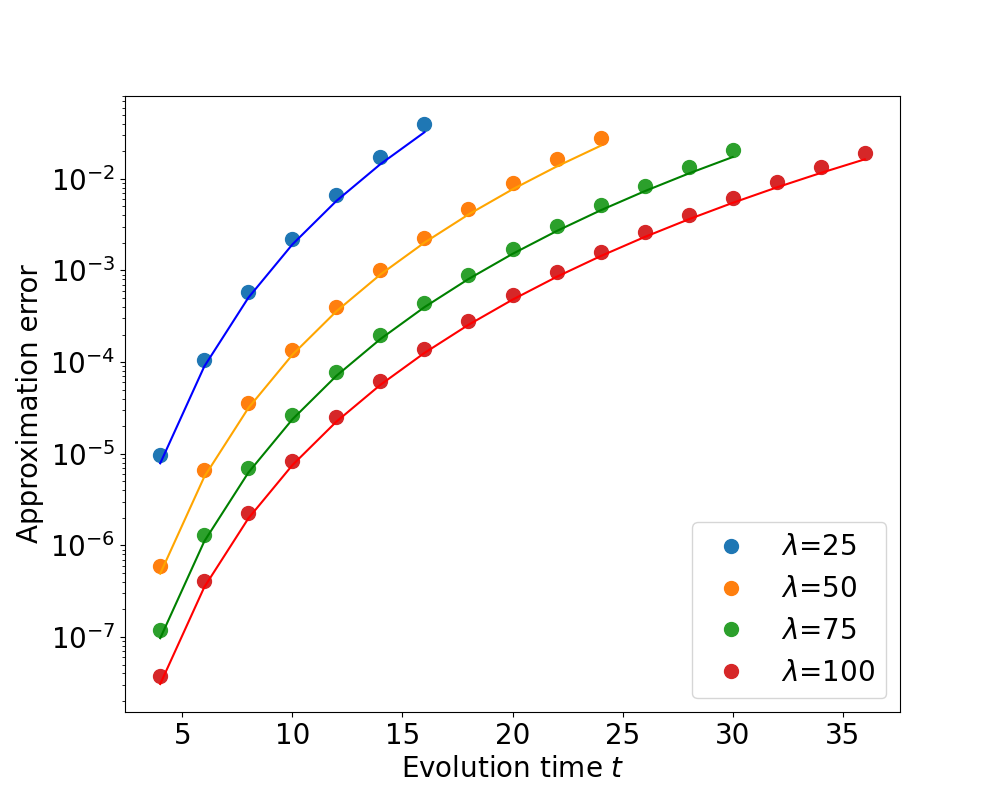
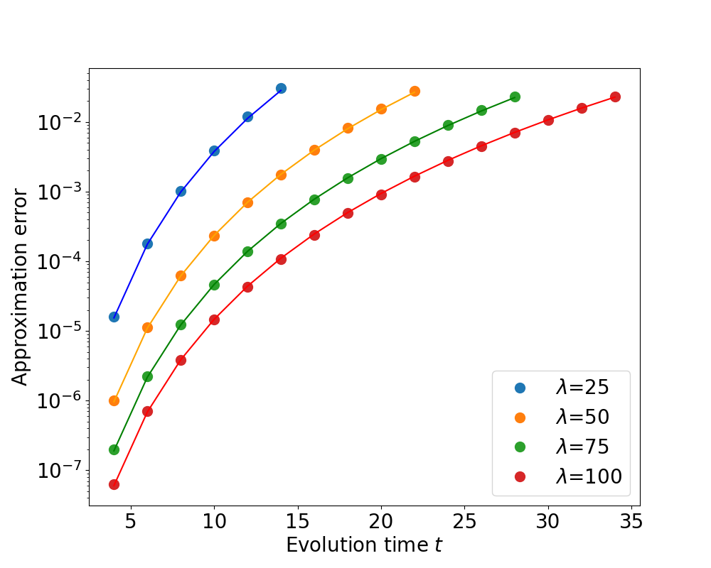
Figure 2 shows a comparison between three types of approximation errors: (1) Trotter error ‖ρ⁡(t)−ρ3​(t)‖1\|\rho(t)-\rho_{3}(t)\|_{1} achieved by the best Trotter circuit 𝒮2​(t/k3)k3{\cal S}_{2}(t/k_{3})^{k_{3}}, (2) MPF error ‖ρ⁡(t)−μ⁡(t)‖1\|\rho(t)-\mu(t)\|_{1}, and (3) fitting ansatz based on Eq. (18). The latter was chosen as

ϵ𝖿𝗂𝗍=0.06​n2​t6​∑i=13|ci|ki4≈(7.5×10⁻⁶)​n2​t6λ4.\epsilon_{\mathsf{fit}}=0.06n^{2}t^{6}\sum_{i=1}^{3}\frac{|c_{i}|}{k_{i}^{4}}\approx\frac{(7.5\times 10^{-6})n^{2}t^{6}}{\lambda^{4}}. (31)

Here we fitted the coefficient a1a_{1} in Eq. (18) by a quadratic function of nn obtaining an estimate a1≈0.06​n2a_{1}\approx 0.06n^{2}. Figure 3 demonstrates that the fitting formula Eq. (31) closely approximates the true MPF error ‖ρ⁡(t)−μ⁡(t)‖1\|\rho(t)-\mu(t)\|_{1} for several values of nn and λ\lambda. The analogous fitting ansatz for the Trotter error ‖ρ⁡(t)−ρk​(t)‖1\|\rho(t)-\rho_{k}(t)\|_{1} with kk steps of the product formula 𝒮2​(t/k){\cal S}_{2}(t/k) was found to be

ϵ𝖿𝗂𝗍′=0.6​n​t3k2.\epsilon^{\prime}_{\mathsf{fit}}=\frac{0.6nt^{3}}{k^{2}}. (32)

One can use Eq. (31) to estimate the number of Trotter steps (and thus the circuit depth) for a given simulation task. For example, solving the benchmark problem of Ref. childs2018toward with n=t=100n=t=100 and error tolerance ϵ𝖿𝗂𝗍=10−3\epsilon_{\mathsf{fit}}=10^{-3} using the second-order MPF would require λ≈3000\lambda\approx 3000 which translates to km​a​x=17​λ≈40,000k_{max}=17\lambda\approx 40,000 Trotter steps.

Refer to caption
Figure 2: Approximation error achieved by the second-order Trotter circuit with k3=850k_{3}=850 time steps (blue) and MPF with (k1,k2,k3)=(200,650,850)(k_{1},k_{2},k_{3})=(200,650,850) (orange) for the Heisenberg spin chain Hamiltonian Eq. (30) with n=14n=14 qubits. Green line shows the fitting formula Eq. (31).
Refer to caption
Refer to caption
Figure 3: Comparison between the true MPF approximation error ‖μ⁡(t)−ρ⁡(t)‖1\|\mu(t)-\rho(t)\|_{1} (circles) and fitting formula Eq. (31) (solid lines) for the second-order product formulas with (k1,k2,k3)=λ⋅(4,13,17)(k_{1},k_{2},k_{3})=\lambda\cdot(4,13,17). Top panel: n=10n=10, Bottom panel: n=14n=14.

Next, consider the fourth-order (p=4p=4) product formula

𝒮4​(t)=(𝒮2​(u​t))2​𝒮2​((1−4​u)​t)​(𝒮2​(u​t))2,{\cal S}_{4}(t)=({\cal S}_{2}(ut))^{2}{\cal S}_{2}((1-4u)t)({\cal S}_{2}(ut))^{2},

where u=14−41/3u=\frac{1}{4-4^{1/3}}, see for instance childs2018toward. Specializing Theorem 1 and Figure 1 to p=4p=4 gives an MPF

μ⁡(t)=∑i=15ci​ρki​(t),\mu(t)=\sum_{i=1}^{5}c_{i}\rho_{k_{i}}(t),

where

(k1,k2,k3,k4,k5)=λ⋅(2,9,17,23,25)(k_{1},k_{2},k_{3},k_{4},k_{5})=\lambda\cdot(2,9,17,23,25)

for an integer λ≥1\lambda\geq 1. Solving the linear system Eq. (17) gives coefficients

c1=1.77273114×10⁻⁸c4=−6.7785310​(5)c2=−0.00267812​(5)c5=7.2808414​(4)c3=0.50036771​(6)\begin{array}[]{cc}c_{1}=1.77273114\times 10^{-8}&c_{4}=-6.7785310(5)\\ c_{2}=-0.00267812(5)&c_{5}=7.2808414(4)\\ c_{3}=0.50036771(6)&\\ \end{array}

Figure 4 shows a comparison between three types of approximation errors: (1) Trotter error ‖ρ⁡(t)−ρ5​(t)‖1\|\rho(t)-\rho_{5}(t)\|_{1} achieved by the best Trotter circuit 𝒮4​(t/k5)k5{\cal S}_{4}(t/k_{5})^{k_{5}}, (2) MPF error ‖ρ⁡(t)−μ⁡(t)‖1\|\rho(t)-\mu(t)\|_{1}, and (3) fitting ansatz based on Eq. (18). The latter was chosen as

ϵ𝖿𝗂𝗍=0.00014​n2​t10​∑i=15|ci|ki8≈(3×10⁻¹⁴)​n2​t10λ8.\epsilon_{\mathsf{fit}}=0.00014n^{2}t^{10}\sum_{i=1}^{5}\frac{|c_{i}|}{k_{i}^{8}}\approx\frac{(3\times 10^{-14})n^{2}t^{10}}{\lambda^{8}}. (33)

Here we fitted the coefficient a1a_{1} in Eq. (18) by a quadratic function of nn obtaining an estimate a1≈0.00014​n2a_{1}\approx 0.00014n^{2}. Figure 5 demonstrates that the fitting formula Eq. (33) closely approximates the true MPF error ‖ρ⁡(t)−μ⁡(t)‖1\|\rho(t)-\mu(t)\|_{1} for several values of nn and λ\lambda and large evolution time tt. Meanwhile, the fitting formula underestimates the error for small tt since it neglects the corrections a2​t2​p+1=a2​t9a_{2}t^{2p+1}=a_{2}t^{9} and a3​t2​p=a3​t8a_{3}t^{2p}=a_{3}t^{8} in the upper bound of Theorem 1. We expect that these correction may become more important for higher-order formulas.

Refer to caption
Figure 4: Approximation error achieved by the fourth-order Trotter circuit with k5=250k_{5}=250 time steps (blue) and MPF with (k1,k2,k3,k4,k5)=(20,90,170,230,250)(k_{1},k_{2},k_{3},k_{4},k_{5})=(20,90,170,230,250) (orange) for the Heisenberg spin chain Hamiltonian Eq. (30) with n=14n=14 qubits. Green line shows the fitting formula Eq. (33).
Refer to caption
Refer to caption
Figure 5: Comparison between the true MPF approximation error ‖μ⁡(t)−ρ⁡(t)‖1\|\mu(t)-\rho(t)\|_{1} (circles) and fitting formula Eq. (33) (solid lines) for the fourth-order product formulas with (k1,k2,k3,k4,k5)=λ⁡(2,9,17,23,25)(k_{1},k_{2},k_{3},k_{4},k_{5})=\lambda(2,9,17,23,25). Top panel: n=10n=10, Bottom panel: n=14n=14. For small evolution time tt the fitting formula underestimates the error since it neglects corrections a2​t2​p+1a_{2}t^{2p+1} and a3​t2​pa_{3}t^{2p} in the upper bound of Theorem 1.

The analogous fitting ansatz for the Trotter error ‖ρ⁡(t)−ρk​(t)‖1\|\rho(t)-\rho_{k}(t)\|_{1} with kk steps of the product formula 𝒮4​(t/k){\cal S}_{4}(t/k) was found to be

ϵ𝖿𝗂𝗍′=0.04​n​t5k4.\epsilon^{\prime}_{\mathsf{fit}}=\frac{0.04nt^{5}}{k^{4}}. (34)

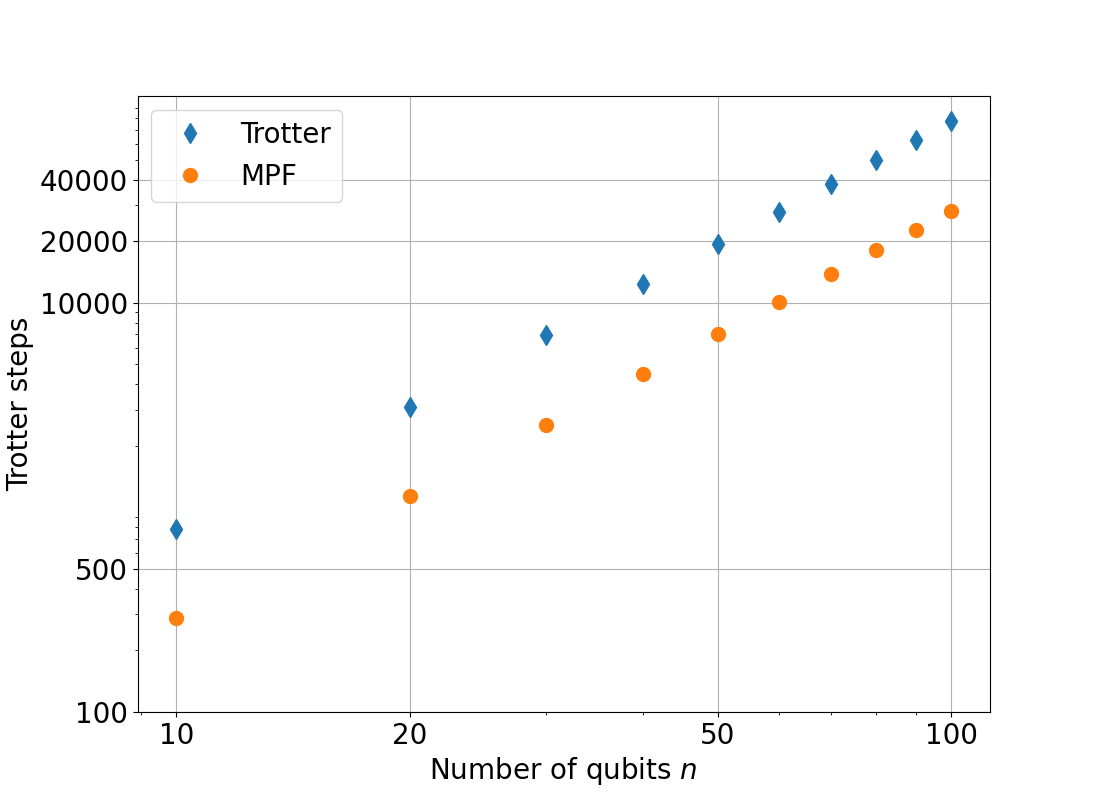
One can use Eq. (33) to estimate the number of Trotter steps for a given simulation task. For example, solving the benchmark problem of Ref. childs2018toward with n=t=100n=t=100 and error tolerance ϵ𝖿𝗂𝗍=10−3\epsilon_{\mathsf{fit}}=10^{-3} using the fourth-order MPF would require λ≈50\lambda\approx 50 which translates to km​a​x=25​λ≈1,250k_{max}=25\lambda\approx 1,250 Trotter steps, as opposed to 40,00040,000 Trotter steps for the second-order MPF. Note however that each Trotter step of 𝒮4{\cal S}_{4} has the same depth as five Trotter steps of 𝒮2{\cal S}_{2}. Thus the fourth-order MPF achieves roughly six-fold depth reduction compared with the second-order MPF.

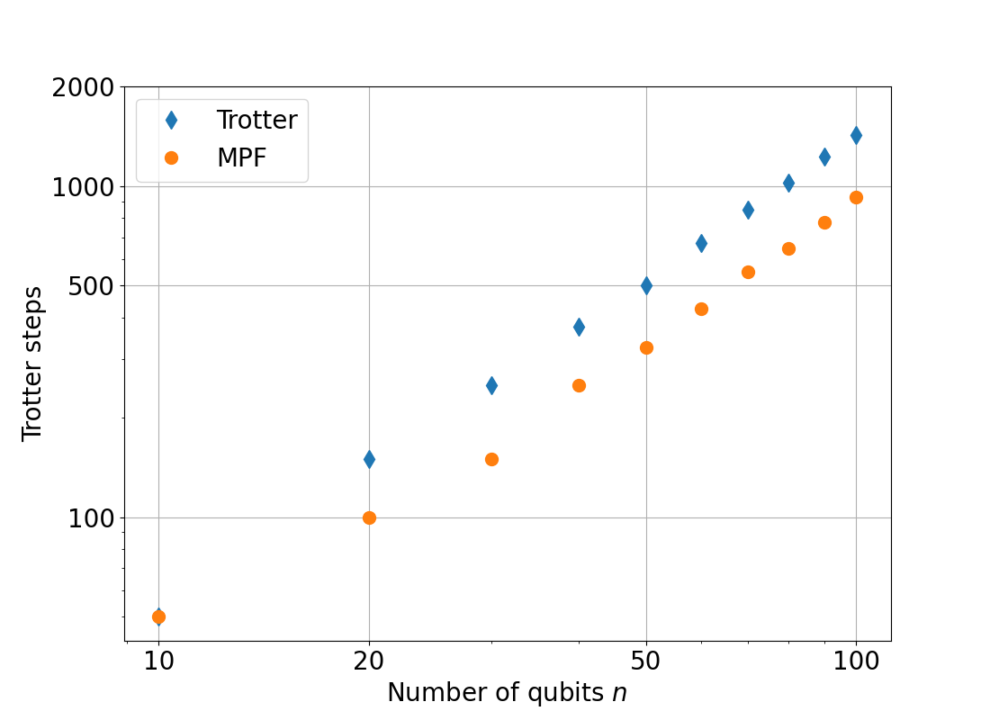
The error tolerance 10−310^{-3} might be too ambitious goal for near-term quantum processors lacking error correction capabilities. Consider a more realistic goal of simulating nn-qubit Hamiltonian Eq. (30) over time interval t=nt=n within 1% error (with respect to the trace norm distance). Combining fitting formulas Eqs. (31,32,33,34) we can compare the number of Trotter steps required to solve this simulation task using (a) second-order and (b) fourth-order Trotter product formulas and their multi-product version. This comparison is presented on Fig. 6.
Refer to caption
Refer to caption
Figure 6: The cost of t=nt=n simulation with the second-order (top panel) and fourth-order (bottom panel) Trotter product formulas and the corresponding MPFs. The cost is measured by the number of Trotter steps required to approximate the time-evolved state ρ⁡(t)\rho(t) within 1% approximation error. MPFs parameters were chosen according to Fig. 1.

Minimax MPFs.

Here we demonstrate the performance of Algorithm 1 with noisy Gram matrix MM and approximated data L𝖺𝗉𝗉𝗋𝗈𝗑L^{\mathsf{approx}} and compare it against the dynamic MPF with exact data (MM and L𝖾𝗑𝖺𝖼𝗍L^{\mathsf{exact}}), static MPF and the best Trotter product formula within MPF. To this end we use the same Hamiltonian as in the previous section, but employ 5 Trotter circuits ρki\rho_{k_{i}} of 2nd order with k→5=(k1,k2,k3,k4,k5)⊤=2⋅(4,10,13,15,17)⊤\vec{k}_{5}=(k_{1},k_{2},k_{3},k_{4},k_{5})^{\top}=2\cdot(4,10,13,15,17)^{\top}. This choice is made to stress one practically important advantage of minimax MPF over the static MPF: the former can provide coefficients of low condition number for any sequence of kik_{i} in contrast to the static MPF, which is sensitive to the choice of kik_{i}: indeed, for the above chosen kik_{i} the resulting Vandermonde matrix (17) is ill-conditioned numerically, hence the vector of coefficients resulting from solving (17), c→(5)=(8.93717538​e−05,−7.30297487​e−01,1.14983897​e+01,−2.73719522​e+01,1.76037706​e+01)⊤\vec{c}^{(5)}=(8.93717538e-05,-7.30297487e-01,1.14983897e+01,-2.73719522e+01,1.76037706e+01)^{\top} has large condition number, ‖c→(5)‖1≈57\|\vec{c}^{(5)}\|_{1}\approx 57. Clearly, c→(5)\vec{c}^{(5)} is impractical since its last three components will amplify sampling noise when computing the linear combination ∑i=15ci(5)​Tr⁡(O​ρki​(t))\sum_{i=1}^{5}c^{(5)}_{i}\tr(O\rho_{k_{i}}(t)) provided Tr⁡(O​ρki​(t))\tr(O\rho_{k_{i}}(t)) is computed on a noisy quantum hardware. However, as noted in Fig. 1, for certain kik_{i} the static MPF formula can be made well-coditioned: e.g. picking a subset of k→5\vec{k}_{5}, namely k→3=2⋅(4,13,17)⊤\vec{k}_{3}=2\cdot(4,13,17)^{\top} one can construct a well-conditioned static MPF with coefficients c→(3)=(0.00612895,−1.55561002,2.54948107)⊤\vec{c}^{(3)}=(0.00612895,-1.55561002,2.54948107)^{\top} and condition number ‖c→(3)‖1≈5\|\vec{c}^{(3)}\|_{1}\approx 5. Below we compare performance of this well-conditioned static MPF given by ∑i=1,ki∈{8,26,34}3ci(3)​ρki\sum_{i=1,k_{i}\in\{8,26,34\}}^{3}c^{(3)}_{i}\rho_{k_{i}} versus dynamic and minimax MPFs corresponding to k→5\vec{k}_{5}: this comparison will make it apparent that minimax MPF allows one to add more of “short depth” Trotter circuits to the linear combination, namely ρ20\rho_{20} and ρ30\rho_{30} in this case, resulting in further improvement of the precision compared to the well-conditioned static MPF with three circuits ρ8,26,34\rho_{8,26,34} without increasing the condition number.

As input for Algorithm 1 we use:

  • •

    t0=1t_{0}=1, d​t=0.05dt=0.05, cFr​(t0)=(0.00612895,0,−1.55561002,0,2.54948107)⊤c^{\mathrm{Fr}}(t_{0})=(0.00612895,0,-1.55561002,0,2.54948107)^{\top}

  • •

    final time TT is such that the Frobenious error of the dynamic MPF with exact data is below 0.310.31,

  • •

    ε=0.01\varepsilon=0.01 and M¯​(t)=M⁡(t)+E1D\bar{M}(t)=M(t)+E_{1}^{D}, A¯​(t)=Q⁡(t)+E2D\bar{A}(t)=Q(t)+E_{2}^{D} where (i,j)(i,j)-component of MM, QQ is computed as per sections IV and IV (we use k0=26k_{0}=26 in section IV), and E1,2DE_{1,2}^{D} are drawn from normal distribution for every time tt such that ‖E1,2D‖2,2≤ε\|E_{1,2}^{D}\|_{2,2}\leq\varepsilon and the components of M¯\bar{M}, A¯\bar{A} are non-negative, M¯\bar{M} has ones on its diagonal.

To compute the coefficients of the dynamic MPF with exact data we minimize quadratic form (IV) over c→:𝟙⊤​c→=1\vec{c}:\mathbb{1}^{\top}\vec{c}=1 for every tj=t0+j​d​tt_{j}=t_{0}+jdt. The dimension of this convex optimization problem is very small: c→\vec{c} has only 5 components; the same observation applies to the convex optimization problem of Algorithm 1. Having this in mind, we solve all those optimization problems by employing Python package cvxpy diamond2016cvxpy. Corresponding snippets of Python code are provided in the Appendix.

Figure 7 provides the comparison: shortly before time t=2t=2 minimax MPF outperforms the best Trotter product formula (k=34k=34), it gets 10×10\times better for t=2.8t=2.8, and around time t=3.9t=3.9 the minimax MPF outperforms the static MPF, it gets 5×5\times better for t=4.5t=4.5, namely when the error of minimax MPF reaches the shot noise magnitude, with condition number ‖c^​(4.5)‖1≈5\|\hat{c}(4.5)\|_{1}\approx 5. Clearly, dynamic MPF with exact data delivers the best performance: about 10000×10000\times better than the static MPF and 100000×100000\times better than the Trotter formula for t=3.29t=3.29. However its condition number is quite high: ‖cFr​(3.29)‖1≈46\|c^{\mathrm{Fr}}(3.29)\|_{1}\approx 46 in contrast to ‖c→3‖1≈5\|\vec{c}_{3}\|_{1}\approx 5 of static MPF and to ‖c^​(3.29)‖1=2.17\|\hat{c}(3.29)\|_{1}=2.17 of the minimax MPF. The difference in performance between dynamic MPF and minimax MPF in the presence of noise is due to the penalization term ε​‖x‖2\varepsilon\|x\|_{2} in Algorithm 1. This term imposes extra constraints on the coefficients, and acts to simultaneously reduce the effect of sampling noise and the condition number of the coefficients. In the presence of shot noise, minimax MPF is therefore more practical than dynamic MPF.

Refer to caption
Figure 7: Approximation error for MPFs: well-conditioned static MPF with ρ8,26,34\rho_{8,26,34} (red), best Trotter formula ρ34\rho_{34} (green), dynamic MPF with exact data (blue) and minimax MPF with noisy/approximated data (orange) both using ρ8,20,26,30,34\rho_{8,20,26,30,34}, for the Heisenberg spin chain Hamiltonian Eq. (30) with n=10n=10 qubits. The shot noise magnitude used to generate M¯,A¯\bar{M},\bar{A} is depicted as a dashed line for reference.

VI Conclusions

To conclude, we studied quantum algorithms for simulating Hamiltonian dynamics based on multi-product formulas. Our first contribution, the upper bound on the approximation error achieved by MPF algorithms of Trotter type for general quantum Hamiltonians which are commonly used in quantum simulations. This upper bound applies to both short and long evolution times overcoming limitations of the previously known bounds. Numerical simulations confirm that our upper bound correctly predicts the approximation error scaling for the considered spin chain Hamiltonian.

Our second contribution, minimax multi-product formula with time-dependent coefficients minimizes Trotter error in Frobenious norm. Minimax MPF is designed to be robust to algorithmic and hardware errors, namely to small additive error in the estimation of overlaps between Trotter circuits which are unavoidable in the experimental implementation due to sampling and hardware noise. Even in the presence of noise minimax MPF outperforms both well-conditioned MPF and the best Trotter formula in numerical simulations. We prove that the worst-case error of minimax MPF scales proportionally to the upper bound of Theorem 1.

A challenging open question is how to extend our bound, Theorem 1, to the case r>p+1r>p+1 and obtain a stronger than quadratic error suppression (in the worst case) compared with the regular product formulas. Likewise, one may ask whether the upper bound of Theorem 1 can be expressed only in terms of low-order nested commutators similar to the bound of Lemma 1.

Acknowledgements

SB thanks Minh Tran, Almudena Vazquez, and Stefan Wörner for helpful discussions. SB was supported in part by the Army Research Office under Grant Number W911NF-20-1-0014.

Appendix A Trotter error for Multi Product Formulas

Proof of Lemma 1

Consider first a single time step, k=1k=1. Then our goal is to upper bound the error ‖ρ1​(t)−ρ⁡(t)‖1\|\rho_{1}(t)-\rho(t)\|_{1} where

ρ⁡(t)=e−i​t​H​ρi​n​ei​t​Handρ1​(t)=𝒮⁡(t)​ρi​n​𝒮​(t)†.\rho(t)=e^{-itH}\rho_{in}e^{itH}\quad\mbox{and}\quad\rho_{1}(t)={\cal S}(t)\rho_{in}{\cal S}(t)^{\dagger}.

Recall that 𝒮(t)=e−i​t​Fd⋯e−i​t​F1{\cal S}(t)=e^{-itF_{d}}\cdots e^{-itF_{1}} is an order-pp product formula associated with a Hamiltonian H=∑a=1dFaH=\sum_{a=1}^{d}F_{a}. Time evolution of 𝒮⁡(t){\cal S}(t) is governed by a time dependent Hamiltonian G⁡(t)G(t) defined as

G⁡(t)=i⁡(d​𝒮​(t)d​t)​𝒮​(t)−1.G(t)=i\left(\frac{d{\cal S}(t)}{dt}\right){\cal S}(t)^{-1}. (35)

The chain rule for derivatives gives

G(t)=Fd+∑a=2de−i​t​Fd⋯e−i​t​FaFa−1ei​t​Fa⋯ei​t​Fd.G(t)=F_{d}+\sum_{a=2}^{d}e^{-itF_{d}}\cdots e^{-itF_{a}}F_{a-1}e^{itF_{a}}\cdots e^{itF_{d}}. (36)

Note that G⁡(0)=∑a=1dFa=HG(0)=\sum_{a=1}^{d}F_{a}=H. A simple algebra shows that

dd​t​(ρ1​(t)−ρ⁡(t))=−i⁡[G⁡(t),ρ1​(t)]+i⁡[H,ρ⁡(t)]=−i⁡[H,ρ1​(t)−ρ⁡(t)]−i⁡[G⁡(t)−H,ρ1​(t)].\frac{d}{dt}(\rho_{1}(t)-\rho(t))=-i[G(t),\rho_{1}(t)]+i[H,\rho(t)]=-i[H,\rho_{1}(t)-\rho(t)]-i[G(t)-H,\rho_{1}(t)].

Here we have added and subtracted a term i​[H,ρ1​(t)]i[H,\rho_{1}(t)] to get the second equality. The above equation is equivalent to

dd​t​(ei​H​t​(ρ1​(t)−ρ⁡(t))​e−i​H​t)=−i​ei​t​H​[G⁡(t)−H,ρ1​(t)]​e−i​t​H.\frac{d}{dt}\left(e^{iHt}(\rho_{1}(t)-\rho(t))e^{-iHt}\right)=-ie^{itH}[G(t)-H,\rho_{1}(t)]e^{-itH}.

Integrating over the interval [0,t][0,t] and noting that ρ1​(0)=ρ​(0)\rho_{1}(0)=\rho(0) gives

ei​H​t(ρ1(t)−ρ(t))e−i​H​t=−i∫0tdt1ei​t1​H[G(t1)−H,ρ1(t)]e−i​t1​H.e^{iHt}(\rho_{1}(t)-\rho(t))e^{-iHt}=-i\int_{0}^{t}dt_{1}e^{it_{1}H}[G(t_{1})-H,\rho_{1}(t)]e^{-it_{1}H}. (37)

Using the unitarity of ei​t​He^{itH} and the triangle inequality one obtains

‖ρ1​(t)−ρ⁡(t)‖1≤∫0td​t1​‖[G⁡(t1)−H,ρ1​(t1)]‖1≤2​∫0td​t1​‖G⁡(t1)−H‖.\|\rho_{1}(t)-\rho(t)\|_{1}\leq\int_{0}^{t}dt_{1}\|\,[G(t_{1})-H,\rho_{1}(t_{1})]\,\|_{1}\leq 2\int_{0}^{t}dt_{1}\|G(t_{1})-H\|. (38)

The second inequality relies on the bound ‖X​Y‖1≤‖X‖⋅‖Y‖1\|XY\|_{1}\leq\|X\|\cdot\|Y\|_{1} which holds for any operators X,YX,Y and the identity ‖ρ1​(t1)‖1=1\|\rho_{1}(t_{1})\|_{1}=1. We shall need the following result which is a rephrasing of Theorem 5 from Ref. childs2021theory.

Fact 1.

Suppose A1,…,As,BA_{1},\ldots,A_{s},B are hermitian operators. Consider an operator-valued function

B(t)=e−i​t​A1⋯e−i​t​AsBei​t​As⋯ei​t​A1B(t)=e^{-itA_{1}}\cdots e^{-itA_{s}}Be^{itA_{s}}\cdots e^{itA_{1}}

and its Taylor series B⁡(t)=∑q=0∞Bq​tqB(t)=\sum_{q=0}^{\infty}B_{q}t^{q} at t=0t=0. Then

‖B⁡(t)−∑q=0p−1Bq​tq‖≤αcomm​(p,A1,…,As,B)​|t|pp!\left\|B(t)-\sum_{q=0}^{p-1}B_{q}t^{q}\right\|\leq\alpha_{\textbf{comm}}(p;A_{1},\ldots,A_{s};B)\frac{|t|^{p}}{p!} (39)

where αcomm​(p,A1,…,As,B)\alpha_{\textbf{comm}}(p;A_{1},\ldots,A_{s};B) is defined in Eq. (II).

Consider Taylor series

G⁡(t)=∑q=0∞Gq​tq.G(t)=\sum_{q=0}^{\infty}G_{q}t^{q}.

We claim that

G0=HandGq=0for 1≤q≤p−1.G_{0}=H\quad\mbox{and}\quad G_{q}=0\quad\mbox{for $1\leq q\leq p-1$}. (40)

Indeed, Eq. (36) gives G0=G⁡(0)=∑a=1dFa=HG_{0}=G(0)=\sum_{a=1}^{d}F_{a}=H. The assumption that 𝒮⁡(t){\cal S}(t) is an order-pp product formula implies that ρ1​(t)−ρ⁡(t)=O⁡(tp+1)\rho_{1}(t)-\rho(t)=O(t^{p+1}) in the limit t→0t\to 0, see Eq. (II). From Eq. (38) one gets G⁡(t)−H=O⁡(tp)G(t)-H=O(t^{p}) in the limit t→0t\to 0. Thus Gq=0G_{q}=0 for 1≤q≤p−11\leq q\leq p-1. Combining Eqs. (36,40) and Fact 1 gives

‖G⁡(t)−H‖=‖G⁡(t)−∑q=0p−1Gq​tq‖≤2​tpp!​∑a=2dαcomm​(p,Fd,…,Fa,Fa−1)=2​αp​tpp!.\|G(t)-H\|=\left\|G(t)-\sum_{q=0}^{p-1}G_{q}t^{q}\right\|\leq\frac{2t^{p}}{p!}\sum_{a=2}^{d}\alpha_{\textbf{comm}}(p;F_{d},\ldots,F_{a};F_{a-1})=\frac{2\alpha_{p}t^{p}}{p!}. (41)

Here we applied Fact 1 to each term e−i​t​Fd⋯e−i​t​FaFa−1ei​t​Fa⋯ei​t​Fde^{-itF_{d}}\cdots e^{-itF_{a}}F_{a-1}e^{itF_{a}}\cdots e^{itF_{d}} in G⁡(t)G(t) with a=2,…,da=2,\ldots,d and used the triangle inequality. Substituting this into Eq. (38) gives

‖ρ1​(t)−ρ⁡(t)‖1≤2​∫0td​t1​2​αp​t1pp!=2​αp​tp+1(p+1)!.\|\rho_{1}(t)-\rho(t)\|_{1}\leq 2\int_{0}^{t}dt_{1}\frac{2\alpha_{p}t_{1}^{p}}{p!}=\frac{2\alpha_{p}t^{p+1}}{(p+1)!}.

This is equivalent to Eq. (10) with a single time step k=1k=1.

Consider now the general case k≥1k\geq 1. Define a sequence of states

σj=𝒮​(t/k)k−j​e−i​t​H​(j/k)​ρi​n​ei​t​H​(j/k)​𝒮​(t/k)−k+j\sigma_{j}={\cal S}(t/k)^{k-j}e^{-itH(j/k)}\rho_{in}e^{itH(j/k)}{\cal S}(t/k)^{-k+j}

where j=0,1,…,kj=0,1,\ldots,k. We have σ0=ρk​(t)\sigma_{0}=\rho_{k}(t) and σk=ρ⁡(t)\sigma_{k}=\rho(t). The norm ‖σj+1−σj‖1\|\sigma_{j+1}-\sigma_{j}\|_{1} can be bounded using Eq. (10) with k=1k=1, evolution time t/kt/k, and the initial state e−i​t​H​(j/k)​ρi​n​ei​t​H​(j/k)e^{-itH(j/k)}\rho_{in}e^{itH(j/k)}. By the triangle inequality,

‖ρk​(t)−ρ⁡(t)‖1=‖σ0−σk‖1≤∑j=0k−1‖σj+1−σj‖1≤2​k​αp​(t/k)p+1(p+1)!=2​αp​tp+1(p+1)!​kp.\|\rho_{k}(t)-\rho(t)\|_{1}=\|\sigma_{0}-\sigma_{k}\|_{1}\leq\sum_{j=0}^{k-1}\|\sigma_{j+1}-\sigma_{j}\|_{1}\leq\frac{2k\alpha_{p}(t/k)^{p+1}}{(p+1)!}=\frac{2\alpha_{p}t^{p+1}}{(p+1)!k^{p}}.

This proves Eq. (10) in the general case.

Proof of Theorem 1

Below we use notations from the previous subsection. Fix evolution time t>0t>0 and the number of time steps kk. Any τ∈[0,t)\tau\in[0,t) can be uniquely written as

τ=τ′+(t/k)​j​(τ)for τ′∈[0,t/k) and integer j⁡(τ)∈[0,k−1].\tau=\tau^{\prime}+(t/k)j(\tau)\quad\mbox{for $\tau^{\prime}\in[0,t/k)$ and integer $j(\tau)\in[0,k-1]$}. (42)

Define an operator valued function

𝒰⁡(τ)=𝒮⁡(τ′)​𝒮​(t/k)j⁡(τ).{\cal U}(\tau)={\cal S}(\tau^{\prime}){\cal S}(t/k)^{j(\tau)}. (43)

By definition, 𝒰⁡(0)=I{\cal U}(0)=I and limτ→t𝒰⁡(τ)=𝒮​(t/k)k\lim_{\tau\to t}{\cal U}(\tau)={\cal S}(t/k)^{k}. Furthermore, for any τ∈[0,t)\tau\in[0,t) which is not an integer multiple of t/kt/k the function 𝒰⁡(τ){\cal U}(\tau) is differentiable and

i​d​𝒰​(τ)d​τ=i​d​𝒮​(τ′)d​τ′​𝒮​(t/k)j⁡(τ)=G⁡(τ′)​𝒮​(τ′)​𝒮​(t/k)j⁡(τ)=G⁡(τ′)​𝒰​(τ).i\frac{d{\cal U}(\tau)}{d\tau}=i\frac{d{\cal S}(\tau^{\prime})}{d\tau^{\prime}}{\cal S}(t/k)^{j(\tau)}=G(\tau^{\prime}){\cal S}(\tau^{\prime}){\cal S}(t/k)^{j(\tau)}=G(\tau^{\prime}){\cal U}(\tau). (44)

Here the second equality uses Eq. (35). Consider a state

σ⁡(τ)=𝒰⁡(τ)​ρi​n​𝒰​(τ)†,0≤τ<t.\sigma(\tau)={\cal U}(\tau)\rho_{in}{\cal U}(\tau)^{\dagger},\qquad 0\leq\tau<t. (45)

By definition,

limτ→tσ⁡(τ)=𝒮​(t/k)k​ρi​n​𝒮​(t/k)−k=ρk​(t).\lim_{\tau\to t}\sigma(\tau)={\cal S}(t/k)^{k}\rho_{in}{\cal S}(t/k)^{-k}=\rho_{k}(t). (46)

Repeating the same arguments as in the derivation of Eq. (37) one gets

ei​τ​AdH(σ(τ)−ρ(τ))=−i∫0τdτ1ei​τ1​AdH[G(τ1′)−H,σ(τ1)].e^{i\tau\mathrm{Ad}_{H}}(\sigma(\tau)-\rho(\tau))=-i\int_{0}^{\tau}d\tau_{1}e^{i\tau_{1}\mathrm{Ad}_{H}}[G(\tau_{1}^{\prime})-H,\sigma(\tau_{1})]. (47)

Adding and subtracting [G⁡(τ1′)−H,ρ⁡(τ1)][G(\tau_{1}^{\prime})-H,\rho(\tau_{1})] in the righthand side gives

ei​τ​AdH​(σ⁡(τ)−ρ⁡(τ))=J1​(τ)−i​∫0τd​τ1​ei​τ1​AdH​[G⁡(τ1′)−H,σ⁡(τ1)−ρ⁡(τ1)],e^{i\tau\mathrm{Ad}_{H}}(\sigma(\tau)-\rho(\tau))=J_{1}(\tau)-i\int_{0}^{\tau}d\tau_{1}e^{i\tau_{1}\mathrm{Ad}_{H}}[G(\tau_{1}^{\prime})-H,\sigma(\tau_{1})-\rho(\tau_{1})], (48)

where

J1(τ)=−i∫0τdτ1ei​τ1​AdH[G(τ1′)−H,ρ(τ1)]J_{1}(\tau)=-i\int_{0}^{\tau}d\tau_{1}e^{i\tau_{1}\mathrm{Ad}_{H}}[G(\tau_{1}^{\prime})-H,\rho(\tau_{1})] (49)

We can now apply Eq. (47) again to express σ⁡(τ1)−ρ⁡(τ1)\sigma(\tau_{1})-\rho(\tau_{1}) in Eq. (48) as an integral. This gives

ei​τ​AdH​(σ⁡(τ)−ρ⁡(τ))=J1​(τ)+J2​(τ),e^{i\tau\mathrm{Ad}_{H}}(\sigma(\tau)-\rho(\tau))=J_{1}(\tau)+J_{2}(\tau), (50)

where

J2(τ)=−∫0τdτ1∫0τ1dτ2[ei​τ1​AdH(G(τ1′)−H),ei​τ2​AdH[G(τ2′)−H,σ(τ2)]].J_{2}(\tau)=-\int_{0}^{\tau}d\tau_{1}\int_{0}^{\tau_{1}}d\tau_{2}[e^{i\tau_{1}\mathrm{Ad}_{H}}(G(\tau_{1}^{\prime})-H),e^{i\tau_{2}\mathrm{Ad}_{H}}[G(\tau_{2}^{\prime})-H,\sigma(\tau_{2})]]. (51)

Using the triangle inequality and normalization ‖σ⁡(τ2)‖1=1\|\sigma(\tau_{2})\|_{1}=1 one gets

‖J2​(τ)‖1≤4​∫0τd​τ1​∫0τ1d​τ2​‖G⁡(τ1′)−H‖⋅‖G⁡(τ2′)−H‖.\|J_{2}(\tau)\|_{1}\leq 4\int_{0}^{\tau}d\tau_{1}\int_{0}^{\tau_{1}}d\tau_{2}\|G(\tau_{1}^{\prime})-H\|\cdot\|G(\tau_{2}^{\prime})-H\|. (52)

Consider the limit τ→t\tau\to t. Dividing the integration domain into kk regions with j⁡(τ1)=j⁡(τ2)j(\tau_{1})=j(\tau_{2}) and (k2){k\choose 2} regions with j⁡(τ1)>j⁡(τ2)j(\tau_{1})>j(\tau_{2}) leads to

‖J2​(t)‖1≤4​k​∫0t/kd​τ1′​∫0τ1d​τ2′​‖G⁡(τ1′)−H‖⋅‖G⁡(τ2′)−H‖+4​(k2)​(∫0t/kd​τ1′​‖G⁡(τ1′)−H‖)2.\|J_{2}(t)\|_{1}\leq 4k\int_{0}^{t/k}d\tau_{1}^{\prime}\int_{0}^{\tau_{1}}d\tau_{2}^{\prime}\|G(\tau_{1}^{\prime})-H\|\cdot\|G(\tau_{2}^{\prime})-H\|+4{k\choose 2}\left(\int_{0}^{t/k}d\tau_{1}^{\prime}\|G(\tau_{1}^{\prime})-H\|\right)^{2}. (53)

From Eq. (41) one gets ‖G⁡(τ1)−H‖≤2​αp​τ1p/p!\|G(\tau_{1})-H\|\leq 2\alpha_{p}\tau_{1}^{p}/p! and ‖G⁡(τ2)−H‖≤2​αp​τ2p/p!\|G(\tau_{2})-H\|\leq 2\alpha_{p}\tau_{2}^{p}/p!. Taking the integrals gives

‖J2​(t)‖1≤(2​k+2​k​(k−1))​(2​αp​tp+1(p+1)!​kp+1)2=2​(2​αp​tp+1(p+1)!​kp)2.\|J_{2}(t)\|_{1}\leq(2k+2k(k-1))\left(\frac{2\alpha_{p}t^{p+1}}{(p+1)!k^{p+1}}\right)^{2}=2\left(\frac{2\alpha_{p}t^{p+1}}{(p+1)!k^{p}}\right)^{2}. (54)

Note that ‖J2​(t)‖1\|J_{2}(t)\|_{1} is proportional to the square of the regular Trotter error, see Eq. (10).

Next let us examine the term J1​(t)J_{1}(t). By definition, ρ⁡(τ1)=e−i​τ1​AdH​ρi​n\rho(\tau_{1})=e^{-i\tau_{1}\mathrm{Ad}_{H}}\rho_{in}. Thus

J1​(t)=−i⁡[L⁡(t),ρi​n]J_{1}(t)=-i[L(t),\rho_{in}] (55)

where

L⁡(t)=∫0td​τ1​ei​τ1​AdH​(G⁡(τ1′)−H).L(t)=\int_{0}^{t}d\tau_{1}e^{i\tau_{1}\mathrm{Ad}_{H}}(G(\tau_{1}^{\prime})-H). (56)

Writing τ1=(t/k)​(v+j)\tau_{1}=(t/k)(v+j) with v∈[0,1)v\in[0,1) and integer j∈[0,k−1]j\in[0,k-1] we get

L⁡(t)=tk​∑j=0k−1∫01d​v​ei​j​(t/k)​AdH​ei​v​(t/k)​AdH​(G⁡(v​t/k)−H).L(t)=\frac{t}{k}\sum_{j=0}^{k-1}\int_{0}^{1}dve^{ij(t/k)\mathrm{Ad}_{H}}e^{iv(t/k)\mathrm{Ad}_{H}}(G(vt/k)-H). (57)

The dependence of L⁡(t)L(t) on 1/k1/k is hard to analyze because kk controls the range of the sum ∑j=0k−1\sum_{j=0}^{k-1}. On the other hand, one should expect that the sum ∑j=0k−1\sum_{j=0}^{k-1} can be well approximated by an integral ∫0k𝑑x\int_{0}^{k}dx. The latter can be transformed to an integral over a range [0,1][0,1] independent of kk by a simple change of variable. A systematic way to approximate a sum by an integral is based on the Euler–Maclaurin formula, see e.g. Theorem D.2.1 in andrews_askey_roy_1999.

Lemma 2 (Euler–Maclaurin formula).

Suppose f⁡(x)f(x) is function with continuous derivatives up to order ss. Let Bs​(x)B_{s}(x) be the Bernoulli polynomial of order ss and Bs=Bs​(0)B_{s}=B_{s}(0) be the Bernoulli number. For example, B0​(x)≡1B_{0}(x)\equiv 1, B1​(x)=x−1/2B_{1}(x)=x-1/2, and B2​(x)=x2−x+1/6B_{2}(x)=x^{2}-x+1/6. Then for any integers j1<j2j_{1}<j_{2} one has

∑j=j1+1j2f⁡(j)=∫j1j2d​x​f​(x)+∑ℓ=1s(−1)ℓ​Bℓℓ!​(f(ℓ−1)​(j2)−f(ℓ−1)​(j1))+(−1)s−1s!​∫j1j2d​x​Bs​(x−[x])​f(s)​(x).\sum_{j=j_{1}+1}^{j_{2}}f(j)=\int_{j_{1}}^{j_{2}}dxf(x)+\sum_{\ell=1}^{s}(-1)^{\ell}\frac{B_{\ell}}{\ell!}\left(f^{(\ell-1)}(j_{2})-f^{(\ell-1)}(j_{1})\right)+\frac{(-1)^{s-1}}{s!}\int_{j_{1}}^{j_{2}}dxB_{s}(x-[x])f^{(s)}(x). (58)

Here f(ℓ)​(x)f^{(\ell)}(x) denotes the ℓ\ell-th derivative of f⁡(x)f(x) and [x][x] denotes the integer part of xx such that x−[x]x-[x] always lies in the interval [0,1)[0,1). Furthermore, for all s≥2s\geq 2

maxx∈[0,1]⁡|Bs​(x)|≤4​s!(2​π)s.\max_{x\in[0,1]}\;|B_{s}(x)|\leq\frac{4s!}{(2\pi)^{s}}. (59)

Consider a function f⁡(x)=ei⁡(x−1)​(t/k)​AdHf(x)=e^{i(x-1)(t/k)\mathrm{Ad}_{H}}. Note that xx is a real variable while f⁡(x)f(x) is a super-operator (a linear map acting on the space of linear operators). We have

f(ℓ)​(x)=(i​t/k)ℓ​(AdH)ℓ​f​(x).f^{(\ell)}(x)=(it/k)^{\ell}(\mathrm{Ad}_{H})^{\ell}f(x).

Applying Eq. (58) with j1=0j_{1}=0 and j2=kj_{2}=k gives

∑j=0k−1ei​j​(t/k)​AdH\displaystyle\sum_{j=0}^{k-1}e^{ij(t/k)\mathrm{Ad}_{H}} =∑j=1kf⁡(j)=∫0kd​x​ei⁡(x−1)​(t/k)​AdH\displaystyle=\sum_{j=1}^{k}f(j)=\int_{0}^{k}dxe^{i(x-1)(t/k)\mathrm{Ad}_{H}} (60)
+∑ℓ=1s(−1)ℓBℓ​(i​t)ℓ−1kℓ−1​ℓ!(ei​t​AdH−I^)e−i⁡(t/k)​AdH(AdH)ℓ−1\displaystyle+\sum_{\ell=1}^{s}(-1)^{\ell}\frac{B_{\ell}(it)^{\ell-1}}{k^{\ell-1}\,\ell!}\left(e^{it\mathrm{Ad}_{H}}-\hat{I}\right)e^{-i(t/k)\mathrm{Ad}_{H}}(\mathrm{Ad}_{H})^{\ell-1}
+(−1)s−1​(i​t)sks​s!∫0kdxBs(x−[x])ei⁡(x−1)​(t/k)​AdH(AdH)s.\displaystyle+\frac{(-1)^{s-1}(it)^{s}}{k^{s}\,s!}\int_{0}^{k}dx\,B_{s}(x-[x])e^{i(x-1)(t/k)\mathrm{Ad}_{H}}(\mathrm{Ad}_{H})^{s}. (61)

Here I^\hat{I} is the identity superoperator. Performing a change of variables x=k​wx=kw with w∈[0,1]w\in[0,1] in the integral over xx and inserting the above expression into Eq. (57) gives

L⁡(t)\displaystyle L(t) =t​∫01d​w​ei​t​w​AdH​∫01d​v​ei⁡(v−1)​(t/k)​AdH​(G⁡(t​v/k)−H)\displaystyle=t\int_{0}^{1}dwe^{itw\mathrm{Ad}_{H}}\int_{0}^{1}dv\,e^{i(v-1)(t/k)\mathrm{Ad}_{H}}(G(tv/k)-H)
−(ei​t​AdH−I^)∑ℓ=1s(−i)ℓBℓ​tℓℓ!∫01dv1kℓ(AdH)ℓ−1ei⁡(v−1)​(t/k)​AdH(G(tv/k)−H)\displaystyle-\left(e^{it\mathrm{Ad}_{H}}-\hat{I}\right)\sum_{\ell=1}^{s}(-i)^{\ell}\frac{B_{\ell}t^{\ell}}{\ell!}\int_{0}^{1}dv\,\frac{1}{k^{\ell}}(\mathrm{Ad}_{H})^{\ell-1}e^{i(v-1)(t/k)\mathrm{Ad}_{H}}(G(tv/k)-H)
−(−i)s​ts+1ks​s!∫01dwei​t​w​AdHBs(kw−[kw])∫01dv(AdH)sei⁡(v−1)​(t/k)​AdH(G(tv/k)−H).\displaystyle-\frac{(-i)^{s}t^{s+1}}{k^{s}\,s!}\int_{0}^{1}dwe^{itw\mathrm{Ad}_{H}}B_{s}(kw-[kw])\int_{0}^{1}dv\,(\mathrm{Ad}_{H})^{s}e^{i(v-1)(t/k)\mathrm{Ad}_{H}}(G(tv/k)-H). (62)

Combining Eqs. (50,54,55,59,62) and using the triangle inequality gives

‖μ⁡(t)−ρ⁡(t)‖1≤2​(ϵ1+ϵ2+ϵ3)+2​(2​αp​tp+1(p+1)!)2​∑i=1r|ci|ki2​p\left\|\mu(t)-\rho(t)\right\|_{1}\leq 2(\epsilon_{1}+\epsilon_{2}+\epsilon_{3})+2\left(\frac{2\alpha_{p}t^{p+1}}{(p+1)!}\right)^{2}\sum_{i=1}^{r}\frac{|c_{i}|}{k_{i}^{2p}} (63)

where

ϵ1=t​maxv∈[0,1]​‖∑j=1rcj​ei⁡(v−1)​(t/kj)​AdH​(G⁡(t​v/kj)−H)‖,\epsilon_{1}=t\max_{v\in[0,1]}\;\left\|\sum_{j=1}^{r}c_{j}e^{i(v-1)(t/k_{j})\mathrm{Ad}_{H}}(G(tv/k_{j})-H)\right\|, (64)
ϵ2=∑ℓ=1s2​Bℓ​tℓℓ!​maxv∈[0,1]​‖∑j=1rcjkjℓ​(AdH)ℓ−1​ei⁡(v−1)​(t/kj)​AdH​(G⁡(t​v/kj)−H)‖\epsilon_{2}=\sum_{\ell=1}^{s}\frac{2B_{\ell}t^{\ell}}{\ell!}\max_{v\in[0,1]}\;\left\|\sum_{j=1}^{r}\frac{c_{j}}{k_{j}^{\ell}}(\mathrm{Ad}_{H})^{\ell-1}e^{i(v-1)(t/k_{j})\mathrm{Ad}_{H}}(G(tv/k_{j})-H)\right\| (65)

and

ϵ3=4​ts+1(2​π)s​maxv∈[0,1]​∑j=1r|cj|kjs⋅‖(AdH)s​ei⁡(v−1)​(t/kj)​AdH​(G⁡(t​v/kj)−H)‖.\epsilon_{3}=\frac{4t^{s+1}}{(2\pi)^{s}}\max_{v\in[0,1]}\;\sum_{j=1}^{r}\frac{|c_{j}|}{k_{j}^{s}}\cdot\|(\mathrm{Ad}_{H})^{s}e^{i(v-1)(t/k_{j})\mathrm{Ad}_{H}}(G(tv/k_{j})-H)\|. (66)

Below we choose

r=p+1ands=p.r=p+1\quad\mbox{and}\quad s=p. (67)

In order to bound ϵ1\epsilon_{1} and ϵ2\epsilon_{2} we have to use condition Eq. (17), that is,

∑j=1rcj=1and∑j=1rcjkjq=0for q∈{p,p+1,…,p+r−2}.\sum_{j=1}^{r}c_{j}=1\quad\mbox{and}\quad\sum_{j=1}^{r}\frac{c_{j}}{k_{j}^{q}}=0\quad\mbox{for $q\in\{p,p+1,\ldots,p+r-2\}$}. (68)

Consider the term ϵ1\epsilon_{1}. Using Eq. (68) one can replace ei⁡(v−1)​(t/kj)​AdH​(G⁡(t​v/kj)−H)e^{i(v-1)(t/k_{j})\mathrm{Ad}_{H}}(G(tv/k_{j})-H) in ϵ1\epsilon_{1} by its Taylor series with all terms of order less than p+r−1=2​pp+r-1=2p omitted. Here the Taylor series are computed with respect to the variable t/kjt/k_{j}. The norm of such truncated Taylor series can be bounded using Fact 1. It gives

ϵ1≤2​t2​p+1(2​p)!​(∑i=1p+1|ci|ki2​p)​∑a=2dαcomm​(2​p,H,Fd,…,Fa,Fa−1).\epsilon_{1}\leq\frac{2t^{2p+1}}{(2p)!}\left(\sum_{i=1}^{p+1}\frac{|c_{i}|}{k_{i}^{2p}}\right)\sum_{a=2}^{d}\alpha_{\textbf{comm}}(2p;H,F_{d},\ldots,F_{a};F_{a-1}). (69)

To bound ϵ2\epsilon_{2} and ϵ3\epsilon_{3} we shall need the following generalization of Fact 1.

Lemma 3.

Suppose A1,…,As,BA_{1},\ldots,A_{s},B are hermitian operators and ℓ≥0\ell\geq 0 is an integer. Consider an operator-valued function

B(t)=(AdA1)ℓe−i​t​AdA1e−i​t​AdA2⋯e−i​t​AdAs(B)B(t)=(\mathrm{Ad}_{A_{1}})^{\ell}e^{-it\mathrm{Ad}_{A_{1}}}e^{-it\mathrm{Ad}_{A_{2}}}\cdots e^{-it\mathrm{Ad}_{A_{s}}}(B)

and its Taylor series B⁡(t)=∑q=0∞Bq​tqB(t)=\sum_{q=0}^{\infty}B_{q}t^{q} at t=0t=0. Define a set of unitary operators

Γ(t)={e−i​τ2​A2⋯e−i​τs​As| 0≤τ2,…,τs≤t}.\Gamma(t)=\{e^{-i\tau_{2}A_{2}}\cdots e^{-i\tau_{s}A_{s}}\,|\,0\leq\tau_{2},\ldots,\tau_{s}\leq t\}.

Then for all t≥0t\geq 0

‖B⁡(t)−∑q=0p−1Bq​tq‖≤tpp!​αcomm​(p,ℓ,A1,…,As,B,t),\left\|B(t)-\sum_{q=0}^{p-1}B_{q}t^{q}\right\|\leq\frac{t^{p}}{p!}\alpha_{\textbf{comm}}(p,\ell;A_{1},\ldots,A_{s};B;t), (70)

with

αcomm​(p,ℓ,A1,…,As,B,t)=∑j1,…,js≥0j1+…+js=pp!j1!⋯js!​maxU∈Γ⁡(t)​‖(AdA1)ℓ+j1​U^​∏γ=2s(AdAγ)jγ​(B)‖.\alpha_{\textbf{comm}}(p,\ell;A_{1},\ldots,A_{s};B;t)=\sum_{\begin{subarray}{c}j_{1},\ldots,j_{s}\geq 0\\ j_{1}+\ldots+j_{s}=p\\ \end{subarray}}\;\;\frac{p!}{j_{1}!\cdots j_{s}!}\;\;\max_{U\in\Gamma(t)}\left\|(\mathrm{Ad}_{A_{1}})^{\ell+j_{1}}\hat{U}\prod_{\gamma=2}^{s}(\mathrm{Ad}_{A_{\gamma}})^{j_{\gamma}}(B)\right\|.

Here U^\hat{U} is a linear map such that U^​(X)=U​X​U−1\hat{U}(X)=UXU^{-1} for all operators XX.

We postpone the proof of the lemma until the end of this section. Consider the term ϵ2\epsilon_{2}. Using Eq. (68) one can replace the operator (AdH)ℓ−1​ei⁡(v−1)​(t/kj)​AdH​(G⁡(t​v/kj)−H)(\mathrm{Ad}_{H})^{\ell-1}e^{i(v-1)(t/k_{j})\mathrm{Ad}_{H}}(G(tv/k_{j})-H) in ϵ2\epsilon_{2} by its Taylor series with all terms of order less than p+r−1−ℓ=2​p−ℓp+r-1-\ell=2p-\ell omitted. The norm of such truncated Taylor series can be bounded using Lemma 3. It gives

ϵ2≤∑ℓ=1p2​Bℓ​t2​pℓ!​(2​p−ℓ)!​(∑j=1p+1|cj|kj2​p)​∑a=2dαcomm​(2​p−ℓ,ℓ−1,H,Fd,…,Fa,Fa−1,t/km​i​n)\epsilon_{2}\leq\sum_{\ell=1}^{p}\frac{2B_{\ell}t^{2p}}{\ell!(2p-\ell)!}\left(\sum_{j=1}^{p+1}\frac{|c_{j}|}{k_{j}^{2p}}\right)\sum_{a=2}^{d}\alpha_{\textbf{comm}}(2p-\ell,\ell-1;H,F_{d},\ldots,F_{a};F_{a-1};t/k_{min}) (71)

Consider the term ϵ3\epsilon_{3} with s=ps=p. The assumption that the base product formula has order pp implies that one can replace the operator (AdH)p​ei⁡(v−1)​(t/kj)​AdH​(G⁡(t​v/kj)−H)(\mathrm{Ad}_{H})^{p}e^{i(v-1)(t/k_{j})\mathrm{Ad}_{H}}(G(tv/k_{j})-H) in ϵ3\epsilon_{3} by its Taylor series with all terms of order less than pp omitted. The norm of such truncated Taylor series can be bounded using Lemma 3. It gives

ϵ3≤4​t2​p+1(2​π)p​p!​(∑j=1p+1|cj|kj2​p)​∑a=2dαcomm​(p,p,H,Fd,…,Fa,Fa−1,t/km​i​n).\epsilon_{3}\leq\frac{4t^{2p+1}}{(2\pi)^{p}p!}\left(\sum_{j=1}^{p+1}\frac{|c_{j}|}{k_{j}^{2p}}\right)\sum_{a=2}^{d}\alpha_{\textbf{comm}}(p,p;H,F_{d},\ldots,F_{a};F_{a-1};t/k_{min}). (72)

Substituting the bounds on ϵ1,ϵ2,ϵ3\epsilon_{1},\epsilon_{2},\epsilon_{3} into Eq. (63) and using the definition of commutator norms βp1,p2\beta_{p_{1},p_{2}}, see Eq. (III,16), completes the proof of Theorem 1.

Proof of Lemma 3

First let us record the well-known integral representation of truncated Taylor series of the exponential function.

Lemma 4 (Taylor’s theorem).

For any operator XX, evolution time t≥0t\geq 0, and integer m≥1m\geq 1 one has

∑q=m∞1q!​(−i​t​AdX)q=(∫0td​τ​μ​(τ)​e−i​τ​AdX)​(−i​t​AdX)mm!\sum_{q=m}^{\infty}\frac{1}{q!}(-it\mathrm{Ad}_{X})^{q}=\left(\int_{0}^{t}d\tau\mu(\tau)e^{-i\tau\mathrm{Ad}_{X}}\right)\frac{(-it\mathrm{Ad}_{X})^{m}}{m!} (73)

where μ⁡(τ)\mu(\tau) is a function satisfying μ⁡(τ)≥0\mu(\tau)\geq 0 and ∫0td​τ​μ​(τ)=1\int_{0}^{t}d\tau\mu(\tau)=1.

Proof.

Applying Taylor’s theorem with integral form of the remainder to the exponential function e−i​t​AdXe^{-it\mathrm{Ad}_{X}} gives

∑q=m∞1q!​(−i​t​AdX)q=(m​t−m​∫0td​τ​(t−τ)m−1​e−i​τ​AdX)​(−i​t​AdX)mm!\sum_{q=m}^{\infty}\frac{1}{q!}(-it\mathrm{Ad}_{X})^{q}=\left(mt^{-m}\int_{0}^{t}d\tau(t-\tau)^{m-1}e^{-i\tau\mathrm{Ad}_{X}}\right)\frac{(-it\mathrm{Ad}_{X})^{m}}{m!}

This is the desired representation with μ⁡(τ)=m​t−m​(t−τ)m−1\mu(\tau)=mt^{-m}(t-\tau)^{m-1}. ∎

Proof of Lemma 3.

First let us introduce some notations. Below we consider ss-tuples of non-negative integers J=(j1,…,js)J=(j_{1},\ldots,j_{s}) satisfying ∑γ=1sjγ=p\sum_{\gamma=1}^{s}j_{\gamma}=p. Let Ωp\Omega_{p} be the set of all such tuples. For any J∈ΩpJ\in\Omega_{p} let m⁡(J)m(J) be largest integer in the range {1,2,…,s}\{1,2,\ldots,s\} such that ∑γ=m⁡(J)sjγ≥p\sum_{\gamma=m(J)}^{s}j_{\gamma}\geq p. Note that jm⁡(J)≥1j_{m(J)}\geq 1 and ∑γ=m⁡(J)+1sjγ≤p−1\sum_{\gamma=m(J)+1}^{s}j_{\gamma}\leq p-1. We use a shorthand J!≡∏γ=1s(jγ)!J!\equiv\prod_{\gamma=1}^{s}(j_{\gamma})!.

We need an upper bound on the norm of the remainder operator R⁡(t)=B⁡(t)−∑q=0p−1Bq​tqR(t)=B(t)-\sum_{q=0}^{p-1}B_{q}t^{q}. Expanding each exponential function that appears in B⁡(t)B(t) in Taylor series gives

R⁡(t)=∑m=1sRm​(t),R(t)=\sum_{m=1}^{s}R_{m}(t),

where

Rm(t)=(AdA1)ℓ∑J∈Ωp:m⁡(J)=m1J!(−itAdA1)j1(−itAdA2)j2⋯(−itAdAs)js(B).R_{m}(t)=(\mathrm{Ad}_{A_{1}})^{\ell}\sum_{J\in\Omega_{p}\,:\,m(J)=m}\;\frac{1}{J!}(-it\mathrm{Ad}_{A_{1}})^{j_{1}}(-it\mathrm{Ad}_{A_{2}})^{j_{2}}\cdots(-it\mathrm{Ad}_{A_{s}})^{j_{s}}(B).

The sum over J∈ΩpJ\in\Omega_{p} with m⁡(J)=mm(J)=m can be rewritten as

∑J∈Ωp:m⁡(J)=m=∑j1=0∞⋯∑jm−1=0∞∑jm+1,…​js≥0jm+1+…+js≤p−1∑jm=p−jm+1−…−js∞.\sum_{J\in\Omega_{p}\,:\,m(J)=m}=\sum_{j_{1}=0}^{\infty}\cdots\sum_{j_{m-1}=0}^{\infty}\;\sum_{\begin{subarray}{c}j_{m+1},\ldots j_{s}\geq 0\\ j_{m+1}+\ldots+j_{s}\leq p-1\\ \end{subarray}}\;\sum_{j_{m}=p-j_{m+1}-\ldots-j_{s}}^{\infty}.

Thus

Rm(t)=(AdA1)ℓe−i​t​AdA1⋯e−i​t​AdAm−1∑jm+1,…​js≥0jm+1+…+js≤p−1∑jm=p−jm+1−…−js∞1jm!⋯js!(−itAdAm)jm(Cjm+1,…,js)R_{m}(t)=(\mathrm{Ad}_{A_{1}})^{\ell}e^{-it\mathrm{Ad}_{A_{1}}}\cdots e^{-it\mathrm{Ad}_{A_{m-1}}}\sum_{\begin{subarray}{c}j_{m+1},\ldots j_{s}\geq 0\\ j_{m+1}+\ldots+j_{s}\leq p-1\\ \end{subarray}}\;\sum_{j_{m}=p-j_{m+1}-\ldots-j_{s}}^{\infty}\frac{1}{j_{m}!\cdots j_{s}!}(-it\mathrm{Ad}_{A_{m}})^{j_{m}}(C_{j_{m+1},\ldots,j_{s}})

where

Cjm+1,…,js=(−itAdAm+1)jm+1⋯(−itAdAs)js(B).C_{j_{m+1},\ldots,j_{s}}=(-it\mathrm{Ad}_{A_{m+1}})^{j_{m+1}}\cdots(-it\mathrm{Ad}_{A_{s}})^{j_{s}}(B).

Applying Lemma 4 to compute the sum over jmj_{m} gives

∑jm=p−jm+1−…−js∞1jm!​(−i​t​AdAm)jm=∫0td​τ​μ​(τ)​e−i​τ​AdAm​(−i​t​AdAm)p−jm+1−…−js(p−jm+1−…−js)!,\sum_{j_{m}=p-j_{m+1}-\ldots-j_{s}}^{\infty}\;\;\frac{1}{j_{m}!}(-it\mathrm{Ad}_{A_{m}})^{j_{m}}=\int_{0}^{t}d\tau\mu(\tau)e^{-i\tau\mathrm{Ad}_{A_{m}}}\frac{(-it\mathrm{Ad}_{A_{m}})^{p-j_{m+1}-\ldots-j_{s}}}{(p-j_{m+1}-\ldots-j_{s})!},

where μ⁡(τ)≥0\mu(\tau)\geq 0 is a normalized probability measure. Plugging this into the formula for Rm​(t)R_{m}(t) one gets

Rm(t)=(−it)p∫0tdτμ(τ)(AdA1)ℓe−i​t​AdA1⋯e−i​t​AdAm−1e−i​τ​AdAm∑j1,…,js≥0j1+…+js=pj1=…=jm−1=0jm≥11J!(AdAm)jm⋯(AdAs)js(B).R_{m}(t)=(-it)^{p}\int_{0}^{t}d\tau\mu(\tau)(\mathrm{Ad}_{A_{1}})^{\ell}e^{-it\mathrm{Ad}_{A_{1}}}\cdots e^{-it\mathrm{Ad}_{A_{m-1}}}e^{-i\tau\mathrm{Ad}_{A_{m}}}\sum_{\begin{subarray}{c}j_{1},\ldots,j_{s}\geq 0\\ j_{1}+\ldots+j_{s}=p\\ j_{1}=\ldots=j_{m-1}=0\\ j_{m}\geq 1\\ \end{subarray}}\;\;\frac{1}{J!}(\mathrm{Ad}_{A_{m}})^{j_{m}}\cdots(\mathrm{Ad}_{A_{s}})^{j_{s}}(B).

Since e−i​t​AdA1e^{-it\mathrm{Ad}_{A_{1}}} commutes with (AdA1)ℓ(\mathrm{Ad}_{A_{1}})^{\ell} and ‖e−i​t​AdA1​(X)‖=‖X‖\|e^{-it\mathrm{Ad}_{A_{1}}}(X)\|=\|X\| for any operator XX, we get

∥Rm(t)|≤tp∑j1,…,js≥0j1+…+js=pj1=…=jm−1=0jm≥11J!maxU∈Γ⁡(t)‖(AdA1)ℓ+j1U^(AdA2)j2⋯(AdAs)js(B)‖.\|R_{m}(t)|\leq t^{p}\sum_{\begin{subarray}{c}j_{1},\ldots,j_{s}\geq 0\\ j_{1}+\ldots+j_{s}=p\\ j_{1}=\ldots=j_{m-1}=0\\ j_{m}\geq 1\\ \end{subarray}}\;\;\frac{1}{J!}\max_{U\in\Gamma(t)}\;\left\|(\mathrm{Ad}_{A_{1}})^{\ell+j_{1}}\hat{U}(\mathrm{Ad}_{A_{2}})^{j_{2}}\cdots(\mathrm{Ad}_{A_{s}})^{j_{s}}(B)\right\|.

The triangle inequality ‖R⁡(t)‖≤∑m=1s‖Rm​(t)‖\|R(t)\|\leq\sum_{m=1}^{s}\|R_{m}(t)\| then gives the desired bound. ∎

Appendix B MPF Trotter error for kk-local spin Hamiltonians

In this section we examine the coefficients a2a_{2} and a3a_{3} that appear in the upper bound of Theorem 1. We specialize the theorem to Hamiltonians HH describing a system of nn qubits with kk-qubit interactions known as kk-local Hamiltonians kitaev2002classical. More precisely, let ℒ⁡(k,J){\cal L}(k,J) be the set of all nn-qubit operators OO that admit a decomposition O=∑αOαO=\sum_{\alpha}O_{\alpha} such that each term OαO_{\alpha} acts non-trivially on at most kk qubits and

∑α:supp⁡(Oα)∋q∥Oα∥≤J\sum_{\alpha\,:\,\mathrm{supp}(O_{\alpha})\ni q}\;\;\|O_{\alpha}\|\leq J

for any qubit qq. Here supp⁡(Oα)\mathrm{supp}(O_{\alpha}) is the support of OαO_{\alpha}, that is, the subset of qubits where OαO_{\alpha} acts non-trivially. Thus the above sum includes all terms OαO_{\alpha} that act non-trivially on a given qubit qq. Hermitian operators in ℒ⁡(k,J){\cal L}(k,J) are kk-local Hamiltonians with an interaction strength JJ. For example, any Hamiltonian describing a DD-dimensional cubic lattice of qubits with bounded-norm interactions supported on elementary cubes is contained in ℒ⁡(2D,J){\cal L}(2^{D},J) for some constant J=O⁡(1)J=O(1). Note that any operator O∈ℒ⁡(k,J)O\in{\cal L}(k,J) obeys

∥O∥≤∑α∥Oα∥≤∑q=1n∑α:supp⁡(Oα)∋q∥Oα∥≤nJ.\|O\|\leq\sum_{\alpha}\|O_{\alpha}\|\leq\sum_{q=1}^{n}\;\sum_{\alpha\,:\,\mathrm{supp}(O_{\alpha})\ni q}\;\;\|O_{\alpha}\|\leq nJ.

Consider an order-pp product formula 𝒮(t)=e−i​t​Fd⋯e−i​t​F2e−i​t​F1{\cal S}(t)=e^{-itF_{d}}\cdots e^{-itF_{2}}e^{-itF_{1}} associated with a Hamiltonian H=∑a=1dFaH=\sum_{a=1}^{d}F_{a}. We assume that p,d=O⁡(1)p,d=O(1) are constants independent of nn, and F1,…,Fd∈ℒ⁡(k,J)F_{1},\ldots,F_{d}\in{\cal L}(k,J) for some constants kk and JJ independent of nn. Furthermore, we assume that each exponent e−i​t​Fae^{-itF_{a}} in the product formula can be implemented by a constant depth circuit. Accordingly, there exists a constant γ=O⁡(1)\gamma=O(1) independent of nn and tt such that e−i​t​AdFae^{-it\mathrm{Ad}_{F_{a}}} maps any single-qubit operator to an operator supported on at most γ\gamma qubits. This setup covers most of quantum spin Hamiltonians studied in physics and Trotter-Suzuki product formulas.

Lemma 5.

Under the above assumptions the coefficients a2a_{2} and a3a_{3} in Theorem 1 scale at most linearly with the number of qubits nn.

Proof.

Let βp,ℓ​(t)\beta_{p,\ell}(t) be the function defined in Eq. (16). Recall that ℓ∈[0,p]\ell\in[0,p] is an integer. By definition, each coefficient a2a_{2} and a3a_{3} is a linear combination of O⁡(1)O(1) terms proportional to βp,ℓ​(t)\beta_{p,\ell}(t) with constant coefficients. Thus it suffices to prove that βp,ℓ​(t)=O​(n)\beta_{p,\ell}(t)=O(n). Using the definition of βp,ℓ​(t)\beta_{p,\ell}(t), it suffices to prove that

‖(AdH)ℓe−i​τd​AdFd⋯e−i​τ1​AdF1(AdFd)qd⋯(AdFa)qa(Fa−1)‖=O(n)\left\|(\mathrm{Ad}_{H})^{\ell}e^{-i\tau_{d}\mathrm{Ad}_{F_{d}}}\cdots e^{-i\tau_{1}\mathrm{Ad}_{F_{1}}}(\mathrm{Ad}_{F_{d}})^{q_{d}}\cdots(\mathrm{Ad}_{F_{a}})^{q_{a}}(F_{a-1})\right\|=O(n) (74)

for any evolution times τi\tau_{i}, integer a∈[2,d]a\in[2,d], and integers qa​…,qd≥0q_{a}\ldots,q_{d}\geq 0 such that qa+…+qd=pq_{a}+\ldots+q_{d}=p. The following proposition controls how locality and interaction strength grow upon taking the commutators.

Proposition 1.

Suppose F1∈ℒ⁡(k1,J1)F_{1}\in{\cal L}(k_{1},J_{1}) and F2∈ℒ⁡(k2,J2)F_{2}\in{\cal L}(k_{2},J_{2}) are arbitrary operators. Then [F1,F2]∈ℒ⁡(k,J)[F_{1},F_{2}]\in{\cal L}(k,J) with k=k1+k2−1k=k_{1}+k_{2}-1 and J=2​J1​J2​(k1+k2)J=2J_{1}J_{2}(k_{1}+k_{2}).

Proof.

Let Fi=∑αFi,αF_{i}=\sum_{\alpha}F_{i,\alpha} be a decompositions of FiF_{i} into kik_{i}-qubit operators Fi,αF_{i,\alpha} such that

∑α:supp⁡(Fi,α)∋q∥Fi,α∥≤Ji\sum_{\alpha\,:\,\mathrm{supp}(F_{i,\alpha})\ni q}\;\;\|F_{i,\alpha}\|\leq J_{i}

for any qubit qq. Then

G:=[F1,F2]=∑α,βGα,β,Gα,β=[F1,α,F2,β].G:=[F_{1},F_{2}]=\sum_{\alpha,\beta}G_{\alpha,\beta},\qquad G_{\alpha,\beta}=[F_{1,\alpha},F_{2,\beta}].

Consider any qubit qq. If q∈supp⁡(Gα,β)q\in\mathrm{supp}(G_{\alpha,\beta}) then q∈supp⁡(F1,α)q\in\mathrm{supp}(F_{1,\alpha}) or q∈supp⁡(F2,β)q\in\mathrm{supp}(F_{2,\beta}). Thus

∑α,β:supp⁡(Gα,β)∋q∥Gα,β∥≤∑α:supp⁡(F1,α)∋q∑β∥Gα,β∥+∑β:supp⁡(F2,β)∋q∑α∥Gα,β∥.\sum_{\alpha,\beta\,:\,\mathrm{supp}(G_{\alpha,\beta})\ni q}\;\;\|G_{\alpha,\beta}\|\leq\sum_{\alpha\,:\,\mathrm{supp}(F_{1,\alpha})\ni q}\;\;\sum_{\beta}\|G_{\alpha,\beta}\|+\sum_{\beta\,:\,\mathrm{supp}(F_{2,\beta})\ni q}\;\;\sum_{\alpha}\|G_{\alpha,\beta}\|. (75)

Clearly Gα,β=0G_{\alpha,\beta}=0 unless supp⁡(F1,α)∩supp⁡(F2,β)≠∅\mathrm{supp}(F_{1,\alpha})\cap\mathrm{supp}(F_{2,\beta})\neq\emptyset. Thus Gα,βG_{\alpha,\beta} has support on at most k1+k2−1k_{1}+k_{2}-1 qubits, that is, GG has locality k1+k2−1k_{1}+k_{2}-1. For any fixed α\alpha one has

∑β∥Gα,β∥≤∑i∈supp⁡(F1,α)∑β:supp⁡(F2,β)∋i  2∥F1,α∥⋅∥F2,β∥≤2J2k1∥F1,α∥.\sum_{\beta}\|G_{\alpha,\beta}\|\leq\sum_{i\in\mathrm{supp}(F_{1,\alpha})}\;\;\sum_{\beta\,:\,\mathrm{supp}(F_{2,\beta})\ni i}\;\;2\|F_{1,\alpha}\|\cdot\|F_{2,\beta}\|\leq 2J_{2}k_{1}\|F_{1,\alpha}\|.

Here we used a bound ‖[F1,α,F2,β]‖≤2​‖F1,α‖⋅‖F2,β‖\|[F_{1,\alpha},F_{2,\beta}]\|\leq 2\|F_{1,\alpha}\|\cdot\|F_{2,\beta}\|. Likewise, for any fixed β\beta one has

∑α∥Gα,β∥≤∑i∈supp⁡(F2,β)∑α:supp⁡(F1,α)∋i  2∥F1,α∥⋅∥F2,β∥≤2J1k2∥F2,β∥.\sum_{\alpha}\|G_{\alpha,\beta}\|\leq\sum_{i\in\mathrm{supp}(F_{2,\beta})}\;\;\sum_{\alpha\,:\,\mathrm{supp}(F_{1,\alpha})\ni i}\;\;2\|F_{1,\alpha}\|\cdot\|F_{2,\beta}\|\leq 2J_{1}k_{2}\|F_{2,\beta}\|.

Substituting this into Eq. (75) one gets

∑α,β:supp⁡(Gα,β)∋q∥Gα,β∥≤2J1J2(k1+k2).\sum_{\alpha,\beta\,:\,\mathrm{supp}(G_{\alpha,\beta})\ni q}\;\;\|G_{\alpha,\beta}\|\leq 2J_{1}J_{2}(k_{1}+k_{2}).

∎

Applying Proposition 1 recursively pp times one infers that

O:=(AdFd)qd⋯(AdFa)qa(Fa−1)∈ℒ(k′,J′)O:=(\mathrm{Ad}_{F_{d}})^{q_{d}}\cdots(\mathrm{Ad}_{F_{a}})^{q_{a}}(F_{a-1})\in{\cal L}(k^{\prime},J^{\prime})

where k′≤k⁡(1+p)k^{\prime}\leq k(1+p) and J′≤J1+p​2p​k​(p+1)J^{\prime}\leq J^{1+p}2^{p}k(p+1). Here we used qa+…+qd=pq_{a}+\ldots+q_{d}=p. Thus we can write

O=∑αOαO=\sum_{\alpha}O_{\alpha}

where OαO_{\alpha} acts non-trivially on at most k′k^{\prime} qubits and

∑α:supp⁡(Oα)∋q∥Oα∥≤J′\sum_{\alpha\,:\,\mathrm{supp}(O_{\alpha})\ni q}\;\;\|O_{\alpha}\|\leq J^{\prime}

for any qubit qq. Define operators

Pα=e−i​τd​AdFd⋯e−i​τ1​AdF1(Oα).P_{\alpha}=e^{-i\tau_{d}\mathrm{Ad}_{F_{d}}}\cdots e^{-i\tau_{1}\mathrm{Ad}_{F_{1}}}(O_{\alpha}).

Unitarity implies ‖Pα‖=‖Oα‖\|P_{\alpha}\|=\|O_{\alpha}\|. Suppose PαP_{\alpha} acts non-trivially on some qubit qq. Then OαO_{\alpha} acts non-trivially on at least one qubit in the backward lightcone of the qubit qq with respect to the circuit e−i​τd​Fd⋯e−i​τ1​F1e^{-i\tau_{d}F_{d}}\cdots e^{-i\tau_{1}F_{1}}. Let this lightcone be LqL_{q}. The assumption that e−i​τ​AdFae^{-i\tau\mathrm{Ad}_{F_{a}}} maps any single-qubit operator to an operator supported on at most γ\gamma qubits implies that |Lq|≤γd|L_{q}|\leq\gamma^{d}. Thus

∑α:supp⁡(Pα)∋q∥Pα∥≤∑i∈Lq∑α:supp⁡(Oα)∋i∥Oα∥≤γdJ′.\sum_{\alpha\,:\,\mathrm{supp}(P_{\alpha})\ni q}\;\;\|P_{\alpha}\|\leq\sum_{i\in L_{q}}\;\sum_{\alpha\,:\,\mathrm{supp}(O_{\alpha})\ni i}\;\;\|O_{\alpha}\|\leq\gamma^{d}J^{\prime}.

The same lightcone argument shows that PαP_{\alpha} acts non-trivially on at most k′​γdk^{\prime}\gamma^{d} qubits. We conclude that

e−i​τd​AdFd⋯e−i​τ1​AdF1(O)∈ℒ(k′′,J′′),e^{-i\tau_{d}\mathrm{Ad}_{F_{d}}}\cdots e^{-i\tau_{1}\mathrm{Ad}_{F_{1}}}(O)\in{\cal L}(k^{\prime\prime},J^{\prime\prime}), (76)

where k′′=γd​k′k^{\prime\prime}=\gamma^{d}k^{\prime} and J′′=γd​J′J^{\prime\prime}=\gamma^{d}J^{\prime}. Finally, we note that H∈ℒ⁡(k,d​J)H\in{\cal L}(k,dJ). Applying Proposition 1 recursively ℓ\ell times one gets

(AdH)ℓe−i​τd​AdFd⋯e−i​τ1​AdF1(AdFd)qd⋯(AdFa)qa(Fa−1)∈ℒ(k′′′,J′′′)(\mathrm{Ad}_{H})^{\ell}e^{-i\tau_{d}\mathrm{Ad}_{F_{d}}}\cdots e^{-i\tau_{1}\mathrm{Ad}_{F_{1}}}(\mathrm{Ad}_{F_{d}})^{q_{d}}\cdots(\mathrm{Ad}_{F_{a}})^{q_{a}}(F_{a-1})\in{\cal L}(k^{\prime\prime\prime},J^{\prime\prime\prime}) (77)

where k′′′≤k′′+k​ℓk^{\prime\prime\prime}\leq k^{\prime\prime}+k\ell and J′′′≤2ℓ​dℓ​Jℓ​J′′​(ℓ​k+k′′)J^{\prime\prime\prime}\leq 2^{\ell}d^{\ell}J^{\ell}J^{\prime\prime}(\ell k+k^{\prime\prime}). Combining all above bounds gives

k′′′≤γd​k​pandJ′′′≤4p+2​p2​dp​J2​p+1​γ2​d​k2.k^{\prime\prime\prime}\leq\gamma^{d}kp\quad\mbox{and}\quad J^{\prime\prime\prime}\leq 4^{p+2}p^{2}d^{p}J^{2p+1}\gamma^{2d}k^{2}.

Clearly, J′′′J^{\prime\prime\prime} is upper bounded by a constant independent of nn. It remains to note that ‖X‖≤n​J′′′\|X\|\leq nJ^{\prime\prime\prime} for any operator X∈ℒ⁡(k′′′,J′′′)X\in{\cal L}(k^{\prime\prime\prime},J^{\prime\prime\prime}). This proves Eq. (74). ∎

Appendix C Proof of Theorem 2

Before introducing the error bound let 𝟙\mathbb{1} denote rr-dimensional vector of ones, let qs=2q_{s}=2 for all s<js<j, provided the final time-step tjt_{j} is such that j>1j>1, and qj=1q_{j}=1, finally set P0=M¯⊤​(t0)​M¯​(t0)+𝟙​𝟙⊤+ε2​IP_{0}=\bar{M}^{\top}(t_{0})\bar{M}(t_{0})+\mathbb{1}\mathbb{1}^{\top}+\varepsilon^{2}I and

Ps\displaystyle P_{s} =𝟙​𝟙⊤+qs​ε2​I+M¯⊤​(ts)​M¯​(ts)\displaystyle=\mathbb{1}\mathbb{1}^{\top}+q_{s}\varepsilon^{2}I+\bar{M}^{\top}(t_{s})\bar{M}(t_{s})
−M¯⊤​(ts)​A¯​(ts)​(Ps−1+A¯⊤​(ts−1)​A¯​(ts−1))−1​A¯⊤​(ts)​M¯​(ts)\displaystyle-\bar{M}^{\top}(t_{s})\bar{A}(t_{s})(P_{s-1}+\bar{A}^{\top}(t_{s-1})\bar{A}(t_{s-1}))^{-1}\bar{A}^{\top}(t_{s})\bar{M}(t_{s})

Note that PjP_{j} is a real symmetric positive-definite r×rr\times r-matrix.

Theorem 2.

Assume that eq. 26 holds and let μS​(t)=∑i=1rci​ρki​(t)\mu^{S}(t)=\sum_{i=1}^{r}c_{i}\rho_{k_{i}}(t) with cic_{i} defined as in Theorem 1. In the setting of Algorithm 1 let

γ⁡(t)=(∑i=1r|ci|ki2​p)​(a1​t2​p+2+a2​t2​p+1+a3​t2​p)+2​αp​(d​t)p+1(p+1)!​k0p\gamma(t)=\left(\sum_{i=1}^{r}\frac{|c_{i}|}{k_{i}^{2p}}\right)(a_{1}t^{2p+2}+a_{2}t^{2p+1}+a_{3}t^{2p})+\frac{2\alpha_{p}(dt)^{p+1}}{(p+1)!k_{0}^{p}}

Let tjt_{j} and c^​(tj)\hat{c}(t_{j}) be defined as in Algorithm 1 and let Ψj=2​ε​‖cFr​(tj)‖2+4​ε​∑s=1j−1‖cFr​(ts)‖2\Psi_{j}=2\varepsilon\|c^{\mathrm{Fr}}(t_{j})\|_{2}+4\varepsilon\sum_{s=1}^{j-1}\|c^{\mathrm{Fr}}(t_{s})\|_{2}. Then for any vector ℓ∈ℝr\ell\in\mathbb{R}^{r} we have:

|ℓ⊤(cFr(tj)−c^(tj)|≤2β^j12⟨Pj+ℓ,ℓ⟩12|\ell^{\top}(c^{\mathrm{Fr}}(t_{j})-\hat{c}(t_{j})|\leq 2\hat{\beta}^{\frac{1}{2}}_{j}\langle P^{+}_{j}\ell,\ell\rangle^{\frac{1}{2}} (78)

Here β^j:=(∑s≤j−1r​γ​(ts)+Ψj)2−αj+⟨Pj​c^​(tj),c^​(tj)⟩\hat{\beta}_{j}:=\left(\sum_{s\leq j-1}\sqrt{r}\gamma(t_{s})+\Psi_{j}\right)^{2}-\alpha_{j}+\langle P_{j}\hat{c}(t_{j}),\hat{c}(t_{j})\rangle{} with r0=𝟙+cFr​(t0)r_{0}=\mathbb{1}+c^{\mathrm{Fr}}(t_{0}), α0=1+cFr​(t0)⊤​cFr​(t0)\alpha_{0}=1+c^{\mathrm{Fr}}(t_{0})^{\top}c^{\mathrm{Fr}}(t_{0}) and

αj=αj−1+1−rj−1⊤​(Pj−1+A¯⊤​(tj−1)​A¯​(tj−1))+​rj−1,rj=M¯⊤​(tj)​A¯​(tj−1)​(Pj−1+A¯⊤​(tj−1)​A¯​(tj−1))+​rj−1+𝟙,\begin{split}&\alpha_{j}=\alpha_{j-1}+1-r_{j-1}^{\top}(P_{j-1}+\bar{A}^{\top}(t_{j-1})\bar{A}(t_{j-1}))^{+}r_{j-1},\\ &r_{j}=\bar{M}^{\top}(t_{j})\bar{A}(t_{j-1})(P_{j-1}+\bar{A}^{\top}(t_{j-1})\bar{A}(t_{j-1}))^{+}r_{j-1}+\mathbb{1},\end{split}

To prove Theorem 2 we need to recall basic results from minimax estimation for linear discrete-time differential-algebraic equations zhuk2010minimax, namely the notion of the minimax estimate. Assume that we are given a vector yy in the form of y=C​φ+ηy=C\varphi+\eta where CC is a given linear transformation of a vector φ\varphi from an abstract Hilbert space ℋ{\cal H} with inner product ⟨⋅,⋅⟩\langle\cdot,\cdot\rangle. We further assume that φ\varphi solves a linear equation L​φ=fL\varphi=f for a given bounded transformation LL, and that ff and η\eta are unknown elements satisfying

G={(f,η):⟨Q1​f,f⟩+⟨Q2​η,η⟩≤1}G=\{(f,\eta):\langle Q_{1}f,f\rangle+\langle Q_{2}\eta,\eta\rangle\leq 1\}

for given symmetric positive definite operators Q1,2Q_{1,2}. The vector φ^∈Gy={φ:⟨Q1​L​φ,L​φ⟩+⟨Q2​(y−C​φ),y−C​φ⟩≤1}\hat{\varphi}\in G_{y}=\{\varphi:\langle Q_{1}L\varphi,L\varphi\rangle+\langle Q_{2}(y-C\varphi),y-C\varphi\rangle\leq 1\} is called a minimax estimate of φ\varphi if

∀ℓ∈ℋ:maxψ∈Gy⁡|⟨ℓ,φ^−ψ⟩|=minφ∈Gy⁡maxψ∈Gy​|⟨ℓ,φ−ψ⟩|\forall\ell\in{\cal H}:\quad\max_{\psi\in G_{y}}|\langle\ell,\hat{\varphi}-\psi\rangle|=\min_{\varphi\in G_{y}}\max_{\psi\in G_{y}}|\langle\ell,\varphi-\psi\rangle| (79)

and ρ^​(ℓ):=maxψ∈Gy⁡|⟨ℓ,φ^−ψ⟩|\hat{\rho}(\ell):=\max_{\psi\in G_{y}}|\langle\ell,\hat{\varphi}-\psi\rangle| is called the minimax error. Clearly, φ^\hat{\varphi} is the minimax or Tchebyshev center of the set of all admissible φ∈Gy\varphi\in G_{y} which are compatible with the uncertainty description given by GG.

Theorem 3 (Theorem 1 from zhuk2010minimax).

Let I⁡(φ):=⟨Q1​L​φ,L​φ⟩+⟨Q2​(y−C​φ),y−C​φ⟩I(\varphi):=\langle Q_{1}L\varphi,L\varphi\rangle+\langle Q_{2}(y-C\varphi),y-C\varphi\rangle. Then the minimax estimate φ^\hat{\varphi} is the unique minimizer of II: φ^∈Argminϕ​I​(ϕ)\hat{\varphi}\in\mathrm{Argmin}_{\phi}I(\phi), and the minimax error is

ρ^(ℓ)=(1−I(φ^))12maxϕ:⟨(L†​Q1​L+C†​Q2​C)​ϕ,ϕ⟩≤1⟨ℓ,ϕ⟩=(1−I(φ^))12⟨(L†Q1L+C†Q2C)−1ℓ,ℓ⟩12\displaystyle\hat{\rho}(\ell)=(1-I(\hat{\varphi}))^{\frac{1}{2}}\max_{\phi:\langle(L^{\dagger}Q_{1}L+C^{\dagger}Q_{2}C)\phi,\phi\rangle\leq 1}\langle\ell,\phi\rangle=(1-I(\hat{\varphi}))^{\frac{1}{2}}\langle(L^{\dagger}Q_{1}L+C^{\dagger}Q_{2}C)^{-1}\ell,\ell\rangle^{\frac{1}{2}}

provided L†​Q1​L+H†​Q2​HL^{\dagger}Q_{1}L+H^{\dagger}Q_{2}H is invertible. Moreover

maxϕ∈Gy⁡‖φ^−ϕ‖=minφ∈Gy⁡maxϕ∈Gy|φ−ϕ|=(1−I⁡(φ^))12​max‖ℓ‖=1​⟨(L†​Q1​L+C†​Q2​C)−1​ℓ,ℓ⟩12\begin{split}&\max_{\phi\in G_{y}}\|\hat{\varphi}-\phi\|=\min_{\varphi\in G_{y}}\max_{\phi\in G_{y}}\|\varphi-\phi\|=(1-I(\hat{\varphi}))^{\frac{1}{2}}\max_{\|\ell\|=1}\langle(L^{\dagger}Q_{1}L+C^{\dagger}Q_{2}C)^{-1}\ell,\ell\rangle^{\frac{1}{2}}\end{split} (80)

Now, let us prove Theorem 2.

Proof of Theorem 2.

Recall the setting of Algorithm 1. The idea of this proof is to construct a set 𝒢y{\cal G}_{y} of all feasible discrete-time trajectories φ=(c→​(t0)​…​c→​(tj))⊤\varphi=(\vec{c}(t_{0})\dots\vec{c}(t_{j}))^{\top}, i.e. all trajectories which satisfy (28) for all possible realizations of E1,2D​(t0)​…​E1,2D​(tj)E^{D}_{1,2}(t_{0})\dots E^{D}_{1,2}(t_{j}), and then demonstrate that the discrete-time trajectory of exact coefficients, φ⋆=(cFr​(t0)​…​cFr​(tj))⊤\varphi^{\star}=(c^{\mathrm{Fr}}(t_{0})\dots c^{\mathrm{Fr}}(t_{j}))^{\top} belongs to 𝒢y{\cal G}_{y} as well as the trajectory φ^=(c^​(t0)​…​c^​(tj))⊤\hat{\varphi}=(\hat{c}(t_{0})\dots\hat{c}(t_{j}))^{\top} generated by Algorithm 1. Then the worst-case error of approximating individual components of φ⋆\varphi^{\star} by corresponding com[onents of φ^\hat{\varphi} as per (79) will be given by (80).

Without loss of generality assume that cFr​(t0)c^{\mathrm{Fr}}(t_{0}) is known. Recall that by assumption the exact matrices M,QM,Q admit the following representation: M⁡(t)∈{M¯​(t)+E1D​(t),‖E1D​(t)‖2,2≤ε}M(t)\in\{\bar{M}(t)+E^{D}_{1}(t),\|E^{D}_{1}(t)\|_{2,2}\leq\varepsilon\} and Q⁡(t)∈{A¯​(t)+E2D​(t),‖E2D​(t)‖2,2≤ε}Q(t)\in\{\bar{A}(t)+E^{D}_{2}(t),\|E^{D}_{2}(t)\|_{2,2}\leq\varepsilon\}, and there exist E1,2⋆E^{\star}_{1,2} such that M⁡(tj)=M¯​(tj)+E1⋆​(tj)M(t_{j})=\bar{M}(t_{j})+E^{\star}_{1}(t_{j}) and Q⁡(tj)=A¯​(tj)+E2⋆​(tj)Q(t_{j})=\bar{A}(t_{j})+E^{\star}_{2}(t_{j}) for some unknown E1,2⋆E^{\star}_{1,2}, see (26) above. Then, adding and substructing E1,2DE^{D}_{1,2} in (28) we find that cFrc^{\mathrm{Fr}} satisfies the following equation:

(M¯​(tj)+E1D)​c→​(tj)\displaystyle(\bar{M}(t_{j})+E^{D}_{1})\vec{c}(t_{j}) =(A¯​(tj)+E2D)​c→​(tj−1)+L𝖾𝗑𝖺𝖼𝗍​(tj)−L𝖺𝗉𝗉𝗋𝗈𝗑​(tj)+(E1D−E1⋆)​cFr​(tj)+(E2⋆−E2D)​cFr​(tj−1)\displaystyle=(\bar{A}(t_{j})+E^{D}_{2})\vec{c}(t_{j-1})+L^{\mathsf{exact}}(t_{j})-L^{\mathsf{approx}}(t_{j})+(E^{D}_{1}-E_{1}^{\star})c^{\mathrm{Fr}}(t_{j})+(E_{2}^{\star}-E^{D}_{2})c^{\mathrm{Fr}}(t_{j-1}) (81)
=(A¯​(tj)+E2D)​c→​(tj−1)+Fj,Fj=(M¯​(tj)+E1D)​cFr​(tj)−(A¯​(tj)+E2D)​cFr​(tj−1)\displaystyle=(\bar{A}(t_{j})+E^{D}_{2})\vec{c}(t_{j-1})+F_{j},\quad F_{j}=(\bar{M}(t_{j})+E^{D}_{1})c^{\mathrm{Fr}}(t_{j})-(\bar{A}(t_{j})+E^{D}_{2})c^{\mathrm{Fr}}(t_{j-1}) (82)

We stress that since cFr,E1,2Dc^{\mathrm{Fr}},E^{D}_{1,2} are not known the term FjF_{j} is treated as an unknown input. The purpose of introducing (81) is to demonstrate that there exist input FjF_{j} such that cFr​(tj)c^{\mathrm{Fr}}(t_{j}) satisfies (81), namely when we set c→=cFr\vec{c}=c^{\mathrm{Fr}} the equation holds (81), hence cFrc^{\mathrm{Fr}} is contained in the set of all c→\vec{c} satisfying (81) while FjF_{j} runs through a set {F:F=(M¯(tj)+E1D)cFr(tj)−(A¯(tj)+E2D)cFr(tj−1),∥E1,2D∥2,2≤ε}\{F:F=(\bar{M}(t_{j})+E^{D}_{1})c^{\mathrm{Fr}}(t_{j})-(\bar{A}(t_{j})+E^{D}_{2})c^{\mathrm{Fr}}(t_{j-1}),\|E^{D}_{1,2}\|_{2,2}\leq\varepsilon\}. Moreover, it is obvious that ‖(M¯​(tj)+E1D)​c→​(tj)−(A¯​(tj)+E2D)​c→​(tj−1)‖2=‖Fj‖2\|(\bar{M}(t_{j})+E^{D}_{1})\vec{c}(t_{j})-(\bar{A}(t_{j})+E^{D}_{2})\vec{c}(t_{j-1})\|_{2}=\|F_{j}\|_{2} hence the discrete-time trajectory φ⋆=(cFr​(t0)​…​cFr​(tj))⊤\varphi^{\star}=(c^{\mathrm{Fr}}(t_{0})\dots c^{\mathrm{Fr}}(t_{j}))^{\top} belongs to the set of all trajectories φ=(c→​(t0)​…​c→​(tj))⊤\varphi=(\vec{c}(t_{0})\dots\vec{c}(t_{j}))^{\top} such that:

‖c→​(t0)−cFr​(t0)‖2+∑s=1j‖(M¯​(ts)+E1D​(ts))​c→​(ts)−(A¯​(ts)+E2D​(ts))​c→​(ts−1)‖2≤∑s=1j‖Fj‖2,𝟙⊤​c→​(ts)=1\displaystyle\|\vec{c}(t_{0})-c^{\mathrm{Fr}}(t_{0})\|_{2}+\sum_{s=1}^{j}\|(\bar{M}(t_{s})+E^{D}_{1}(t_{s}))\vec{c}(t_{s})-(\bar{A}(t_{s})+E^{D}_{2}(t_{s}))\vec{c}(t_{s-1})\|_{2}\leq\sum_{s=1}^{j}\|F_{j}\|_{2},\quad\mathbb{1}^{\top}\vec{c}(t_{s})=1 (83)

Using sub-multiplicativity of the matrix norm ∥⋅∥2,2\|\cdot\|_{2,2} we find:

‖(M¯​(tj)+E1D)​c→​(tj)−(A¯​(tj)+E2D)​c→​(tj−1)‖2\displaystyle\|(\bar{M}(t_{j})+E^{D}_{1})\vec{c}(t_{j})-(\bar{A}(t_{j})+E^{D}_{2})\vec{c}(t_{j-1})\|_{2} ≤‖M¯​(tj)​c→​(tj)−A¯​(tj)​c→​(tj−1)‖2+‖E1D‖2,2​‖c→​(ts)‖2+‖E2D‖2,2​‖c→​(ts−1)‖2\displaystyle\leq\|\bar{M}(t_{j})\vec{c}(t_{j})-\bar{A}(t_{j})\vec{c}(t_{j-1})\|_{2}+\|E^{D}_{1}\|_{2,2}\|\vec{c}(t_{s})\|_{2}+\|E^{D}_{2}\|_{2,2}\|\vec{c}(t_{s-1})\|_{2}
≤‖M¯​(tj)​c→​(tj)−A¯​(tj)​c→​(tj−1)‖2+ε​‖c→​(ts)‖2+ε​‖c→​(ts−1)‖2\displaystyle\leq\|\bar{M}(t_{j})\vec{c}(t_{j})-\bar{A}(t_{j})\vec{c}(t_{j-1})\|_{2}+\varepsilon\|\vec{c}(t_{s})\|_{2}+\varepsilon\|\vec{c}(t_{s-1})\|_{2}

and this upper-bound is attained at

E¯1D​(ts)=ε​[M¯​(ts)​c→​(ts)−(A¯​(ts)+E2D​(ts))​c→​(ts−1)]​c→⊤​(ts)‖M¯​(ts)​c→​(ts)−(A¯​(ts)+E2D​(ts))​c→​(ts−1)‖2​‖c→​(ts)‖2,E¯2D​(ts)=ε​[M¯​(ts)​c→​(ts)−A¯​(ts)​c→​(ts−1)]​c→⊤​(ts−1)‖M¯​(ts)​c→​(ts)−A¯​(ts)​c→​(ts−1)‖2​‖c→​(ts−1)‖2\bar{E}_{1}^{D}(t_{s})=\varepsilon\frac{\bigl[\bar{M}(t_{s})\vec{c}(t_{s})-(\bar{A}(t_{s})+E^{D}_{2}(t_{s}))\vec{c}(t_{s-1})\bigr]\vec{c}^{\top}(t_{s})}{\|\bar{M}(t_{s})\vec{c}(t_{s})-(\bar{A}(t_{s})+E^{D}_{2}(t_{s}))\vec{c}(t_{s-1})\|_{2}\|\vec{c}(t_{s})\|_{2}},\quad\bar{E}_{2}^{D}(t_{s})=\varepsilon\frac{\bigl[\bar{M}(t_{s})\vec{c}(t_{s})-\bar{A}(t_{s})\vec{c}(t_{s-1})\bigr]\vec{c}^{\top}(t_{s-1})}{\|\bar{M}(t_{s})\vec{c}(t_{s})-\bar{A}(t_{s})\vec{c}(t_{s-1})\|_{2}\|\vec{c}(t_{s-1})\|_{2}}

Indeed, simple algebra shows that ‖E¯1,2D‖2,2=ε\|\bar{E}_{1,2}^{D}\|_{2,2}=\varepsilon and

‖(M¯​(tj)+E¯1D)​c→​(tj)−(A¯​(tj)+E¯2D)​c→​(tj−1)‖2=‖M¯​(tj)​c→​(tj)−A¯​(tj)​c→​(tj−1)‖2+ε​‖c→​(ts)‖2+ε​‖c→​(ts−1)‖2\|(\bar{M}(t_{j})+\bar{E}^{D}_{1})\vec{c}(t_{j})-(\bar{A}(t_{j})+\bar{E}^{D}_{2})\vec{c}(t_{j-1})\|_{2}=\|\bar{M}(t_{j})\vec{c}(t_{j})-\bar{A}(t_{j})\vec{c}(t_{j-1})\|_{2}+\varepsilon\|\vec{c}(t_{s})\|_{2}+\varepsilon\|\vec{c}(t_{s-1})\|_{2}

In other words the worst-case realization of the matrices E1,2DE_{1,2}^{D} are given by the trajectories E¯1,2D​(ts)\bar{E}_{1,2}^{D}(t_{s}), and for this worst-case scenario (83) takes the following form:

‖c→​(t0)−cFr​(t0)‖2+∑s=1j(‖M¯​(ts)​c→​(ts)−A¯​(ts)​c→​(ts−1)‖2+ε​‖c→​(ts)‖2+ε​‖c→​(ts−1)‖2)≤∑s=1j‖F¯j‖2,𝟙⊤​c→​(ts)=1\displaystyle\|\vec{c}(t_{0})-c^{\mathrm{Fr}}(t_{0})\|_{2}+\sum_{s=1}^{j}\bigl(\|\bar{M}(t_{s})\vec{c}(t_{s})-\bar{A}(t_{s})\vec{c}(t_{s-1})\|_{2}+\varepsilon\|\vec{c}(t_{s})\|_{2}+\varepsilon\|\vec{c}(t_{s-1})\|_{2}\bigr)\leq\sum_{s=1}^{j}\|\bar{F}_{j}\|_{2},\quad\mathbb{1}^{\top}\vec{c}(t_{s})=1 (84)

provided F¯j=(M¯+E¯1D)​cFr​(tj)−(A¯+E¯2D)​cFr​(tj−1)\bar{F}_{j}=(\bar{M}+\bar{E}^{D}_{1})c^{\mathrm{Fr}}(t_{j})-(\bar{A}+\bar{E}^{D}_{2})c^{\mathrm{Fr}}(t_{j-1}). Setting c→=cFr\vec{c}=c^{\mathrm{Fr}} in the definition of E¯1,2D​(ts)\bar{E}_{1,2}^{D}(t_{s}) we find:

F¯j=‖M¯​(ts)​cFr​(ts)−A¯​(ts)​cFr​(ts−1)‖2+ε​‖cFr​(ts)‖2+ε​‖cFr​(ts−1)‖2\bar{F}_{j}=\|\bar{M}(t_{s})c^{\mathrm{Fr}}(t_{s})-\bar{A}(t_{s})c^{\mathrm{Fr}}(t_{s-1})\|_{2}+\varepsilon\|c^{\mathrm{Fr}}(t_{s})\|_{2}+\varepsilon\|c^{\mathrm{Fr}}(t_{s-1})\|_{2}

hence we can further restrict the set (84) of all feasible trajectories φ\varphi to the following set:

𝒢={φ:∥c→0−cFr(t0)∥2\displaystyle{\cal G}=\{\varphi:\|\vec{c}_{0}-c^{\mathrm{Fr}}(t_{0})\|_{2} +∑s=1j(∥M¯(ts)c→(ts)−A¯(ts)c→(ts−1)∥2+ε∥c→(ts)∥2+ε∥c→(ts−1)∥2)≤Σj,𝟙⊤c→(ts)=1,\displaystyle+\sum_{s=1}^{j}\bigl(\|\bar{M}(t_{s})\vec{c}(t_{s})-\bar{A}(t_{s})\vec{c}(t_{s-1})\|_{2}+\varepsilon\|\vec{c}(t_{s})\|_{2}+\varepsilon\|\vec{c}(t_{s-1})\|_{2}\bigr)\leq\Sigma_{j},\mathbb{1}^{\top}\vec{c}(t_{s})=1, (85)
Σj=∑s=1j(∥M¯(ts)cFr(ts)−A¯(ts)cFr(ts−1)∥2+ε∥cFr(ts)∥2+ε∥cFr(ts−1)∥2)}\displaystyle\Sigma_{j}=\sum_{s=1}^{j}\bigl(\|\bar{M}(t_{s})c^{\mathrm{Fr}}(t_{s})-\bar{A}(t_{s})c^{\mathrm{Fr}}(t_{s-1})\|_{2}+\varepsilon\|c^{\mathrm{Fr}}(t_{s})\|_{2}+\varepsilon\|c^{\mathrm{Fr}}(t_{s-1})\|_{2}\bigr)\} (86)

Clearly, φ⋆∈𝒢\varphi^{\star}\in{\cal G}: indeed, substituting φ=φ⋆\varphi=\varphi^{\star} the inequality in the 1st line of the definition of 𝒢{\cal G} becomes exact. Note that φ^∈𝒢\hat{\varphi}\in{\cal G}: indeed, by construction of φ^\hat{\varphi} the inequality in the 1st line of the definition of 𝒢{\cal G} is strict. Finally, since ∥⋅∥2≤∥⋅∥1\|\cdot\|_{2}\leq\|\cdot\|_{1} it follows that

‖c→​(t0)−cFr​(t0)‖22\displaystyle\|\vec{c}(t_{0})-c^{\mathrm{Fr}}(t_{0})\|^{2}_{2} +∑s=1j(∥M¯(ts)c→(ts)−A¯(ts)c→(ts−1)∥22+ε2∥c→(ts)∥22+ε2∥c→(ts−1)∥22)\displaystyle+\sum_{s=1}^{j}\bigl(\|\bar{M}(t_{s})\vec{c}(t_{s})-\bar{A}(t_{s})\vec{c}(t_{s-1})\|^{2}_{2}+\varepsilon^{2}\|\vec{c}(t_{s})\|^{2}_{2}+\varepsilon^{2}\|\vec{c}(t_{s-1})\|_{2}^{2}\bigr)
≤(∥c→0−cFr(t0)∥2+∑s=1j(∥(M¯(ts)c→(ts)−A¯(ts)c→(ts−1)∥2+ε∥c→(ts)∥2+ε∥c→(ts−1)∥2))2≤Σj2\displaystyle\leq\left(\|\vec{c}_{0}-c^{\mathrm{Fr}}(t_{0})\|_{2}+\sum_{s=1}^{j}\bigl(\|(\bar{M}(t_{s})\vec{c}(t_{s})-\bar{A}(t_{s})\vec{c}(t_{s-1})\|_{2}+\varepsilon\|\vec{c}(t_{s})\|_{2}+\varepsilon\|\vec{c}(t_{s-1})\|_{2}\bigr)\right)^{2}\leq\Sigma_{j}^{2}

hence both φ⋆=(cFr​(t0)​…​cFr​(tj))⊤\varphi^{\star}=(c^{\mathrm{Fr}}(t_{0})\dots c^{\mathrm{Fr}}(t_{j}))^{\top} and φ^=(c→​(t0)​…​c→​(tj))⊤\hat{\varphi}=(\vec{c}(t_{0})\dots\vec{c}(t_{j}))^{\top} belong to the set:

𝒢~y={φ\displaystyle\tilde{\cal G}_{y}=\{\varphi =(c→​(t0)​…​c→​(tj))⊤:‖c→​(t0)−cFr​(t0)‖22+ε2​‖c→​(t0)‖22+∑s=1j‖M¯​(ts)​c→​(ts)−A¯​(ts)​c→​(ts−1)‖22\displaystyle=(\vec{c}(t_{0})\dots\vec{c}(t_{j}))^{\top}:\|\vec{c}(t_{0})-c^{\mathrm{Fr}}(t_{0})\|^{2}_{2}+\varepsilon^{2}\|\vec{c}(t_{0})\|^{2}_{2}+\sum_{s=1}^{j}\|\bar{M}(t_{s})\vec{c}(t_{s})-\bar{A}(t_{s})\vec{c}(t_{s-1})\|^{2}_{2} (87)
+ε2∥c→(tj)∥22+2ε2∑s=1j−1∥c→(ts)∥22≤Σj2,𝟙⊤c→(ts)=1}\displaystyle+\varepsilon^{2}\|\vec{c}(t_{j})\|_{2}^{2}+2\varepsilon^{2}\sum_{s=1}^{j-1}\|\vec{c}(t_{s})\|^{2}_{2}\leq\Sigma_{j}^{2},\quad\mathbb{1}^{\top}\vec{c}(t_{s})=1\} (88)

Define C⁡(α)=(𝟙⊤α​I)C(\alpha)=\bigl(\begin{smallmatrix}\mathbb{1}^{\top}\\ \alpha I\end{smallmatrix}\bigr) and y~=(1,0,…,0)⊤\tilde{y}=(1,0,\dots,0)^{\top} so that ‖y~−C⁡(α)​c→​(ts)‖22=(1−𝟙⊤​c→​(ts))2+α2​‖c→​(ts)‖22\|\tilde{y}-C(\alpha)\vec{c}(t_{s})\|_{2}^{2}=(1-\mathbb{1}^{\top}\vec{c}(t_{s}))^{2}+\alpha^{2}\|\vec{c}(t_{s})\|^{2}_{2}. Using this notations we can rewrite (87) in a more compact form: let 𝒞j=diag⁡(C⁡(ε2),C⁡(2​ε2),…,C⁡(2​ε2),C⁡(ε2)){\cal C}_{j}=\operatorname{diag}(C(\varepsilon^{2}),C(\sqrt{2}\varepsilon^{2}),\dots,C(\sqrt{2}\varepsilon^{2}),C(\varepsilon^{2})), yj=(y~​…,y~)⊤y_{j}=(\tilde{y}\dots,\tilde{y})^{\top}, bj=(cFr​(t0),0,…​0)⊤b_{j}=(c^{\mathrm{Fr}}(t_{0}),0,\dots 0)^{\top} and set

Lj=[I00…00−A¯​(t0)M¯​(t0)0…000−A¯​(t1)M¯​(t1)…00000…−A¯​(tj)M¯​(tj)]L_{j}=\left[\begin{smallmatrix}I&&0&&0&&\ldots&&0&&0\\ -\bar{A}(t_{0})&&\bar{M}(t_{0})&&0&&\ldots&&0&&0\\ 0&&-\bar{A}(t_{1})&&\bar{M}(t_{1})&&\ldots&&0&&0\\ \vdots&&\vdots&&\vdots&&\vdots&&\vdots&&\vdots\\ 0&&0&&0&&\ldots&&-\bar{A}(t_{j})&&\bar{M}(t_{j})\end{smallmatrix}\right] (89)

Clearly, every element of (87) belongs to the following set 𝒢y{\cal G}_{y}, which is in fact just a compact way of writing (87) but with the hard constraint 𝟙⊤​c→​(ts)=1\mathbb{1}^{\top}\vec{c}(t_{s})=1 relaxed as (1−𝟙⊤​c→​(ts))2(1-\mathbb{1}^{\top}\vec{c}(t_{s}))^{2}:

𝒢y={φ:‖Lj​φ−bj‖22+‖y−𝒞j​φ‖22≤Σj2}{\cal G}_{y}=\{\varphi:\|L_{j}\varphi-b_{j}\|_{2}^{2}+\|y-{\cal C}_{j}\varphi\|_{2}^{2}\leq\Sigma_{j}^{2}\} (90)

Now, as we saw above both φ⋆=(cFr​(t0)​…​cFr​(tj))⊤\varphi^{\star}=(c^{\mathrm{Fr}}(t_{0})\dots c^{\mathrm{Fr}}(t_{j}))^{\top} and φ^=(c→​(t0)​…​c→​(tj))⊤\hat{\varphi}=(\vec{c}(t_{0})\dots\vec{c}(t_{j}))^{\top} belong to 𝒢y{\cal G}_{y} hence the worst-case error of this trajectory is given by the largest diameter of 𝒢y{\cal G}_{y}. To compute the latter let us first note that by (28):

‖(M¯​(ts)±E1⋆)​cFr​(ts)−(A¯​(ts)±E2⋆)​cFr​(ts−1)‖2≤‖L𝖾𝗑𝖺𝖼𝗍​(ts)−L𝖺𝗉𝗉𝗋𝗈𝗑​(ts)‖2+ε​‖cFr​(ts)‖2+ε​‖cFr​(ts−1)‖2\|(\bar{M}(t_{s})\pm E_{1}^{\star})c^{\mathrm{Fr}}(t_{s})-(\bar{A}(t_{s})\pm E_{2}^{\star})c^{\mathrm{Fr}}(t_{s-1})\|_{2}\leq\|L^{\mathsf{exact}}(t_{s})-L^{\mathsf{approx}}(t_{s})\|_{2}+\varepsilon\|c^{\mathrm{Fr}}(t_{s})\|_{2}+\varepsilon\|c^{\mathrm{Fr}}(t_{s-1})\|_{2}

hence

Σj≤2​ε​‖cFr​(tj)‖2+∑s=1j‖L𝖾𝗑𝖺𝖼𝗍​(tj)−L𝖺𝗉𝗉𝗋𝗈𝗑​(tj)‖2+4​ε​∑s=1j−1‖cFr​(ts)‖2\Sigma_{j}\leq 2\varepsilon\|c^{\mathrm{Fr}}(t_{j})\|_{2}+\sum_{s=1}^{j}\|L^{\mathsf{exact}}(t_{j})-L^{\mathsf{approx}}(t_{j})\|_{2}+4\varepsilon\sum_{s=1}^{j-1}\|c^{\mathrm{Fr}}(t_{s})\|_{2}

and let’s estimate ‖L𝖾𝗑𝖺𝖼𝗍​(tj)−L𝖺𝗉𝗉𝗋𝗈𝗑​(tj)‖2\|L^{\mathsf{exact}}(t_{j})-L^{\mathsf{approx}}(t_{j})\|_{2}. To this end recall that ρ𝖺𝗉𝗉𝗋𝗈𝗑​(tj)=𝒮​(d​t/k0)k0​μD​(tj−1)​𝒮​(d​t/k0)−k0\rho^{\mathsf{approx}}(t_{j})={\cal S}(dt/k_{0})^{k_{0}}\mu^{D}(t_{j-1}){\cal S}(dt/k_{0})^{-k_{0}} and μD​(t)=∑i=1rciFr​(t)​ρki​(t)\mu^{D}(t)=\sum_{i=1}^{r}c^{\mathrm{Fr}}_{i}(t)\rho_{k_{i}}(t). Noting that ‖ρki​(tj)‖∞=1\|\rho_{k_{i}}(t_{j})\|_{\infty}=1 and ‖ρki​(tj)‖∞=1\|\rho_{k_{i}}(t_{j})\|_{\infty}=1 we have:

|Li𝖾𝗑𝖺𝖼𝗍(tj)\displaystyle|L_{i}^{\mathsf{exact}}(t_{j}) −Li𝖺𝗉𝗉𝗋𝗈𝗑​(tj)|=|Tr⁡((ρ⁡(tj)−ρ𝖺𝗉𝗉𝗋𝗈𝗑​(tj))​ρki​(tj))|=|Tr⁡((e−i​H​d​t​ρ​(tj−1)​ei​H​d​t−ρ𝖺𝗉𝗉𝗋𝗈𝗑​(tj))​ρki​(tj))|\displaystyle-L_{i}^{\mathsf{approx}}(t_{j})|=|\tr\bigl((\rho(t_{j})-\rho^{\mathsf{approx}}(t_{j}))\rho_{k_{i}}(t_{j})\bigr)|=|\tr\bigl((e^{-iHdt}\rho(t_{j-1})e^{iHdt}-\rho^{\mathsf{approx}}(t_{j}))\rho_{k_{i}}(t_{j})\bigr)|
≤|Tr⁡((e−i​H​d​t​(ρ⁡(tj−1)−μD​(tj−1))​ei​H​d​t​ρki​(tj))|+|Tr⁡((e−i​H​d​t​μD​(tj−1)​ei​H​d​t−ρ𝖺𝗉𝗉𝗋𝗈𝗑​(tj))​ρki​(tj))|CLOSE\displaystyle\leq|\tr\bigl((e^{-iHdt}(\rho(t_{j-1})-\mu^{D}(t_{j-1}))e^{iHdt}\rho_{k_{i}}(t_{j})\bigr)|+|\tr\bigl((e^{-iHdt}\mu^{D}(t_{j-1})e^{iHdt}-\rho^{\mathsf{approx}}(t_{j}))\rho_{k_{i}}(t_{j})\bigr)|
≤‖e−i​H​d​t​(ρ⁡(tj−1)−μD​(tj−1))​ei​H​d​t‖2​‖ρki​(tj)‖2+‖e−i​H​d​t​μD​(tj−1)​ei​H​d​t−ρ𝖺𝗉𝗉𝗋𝗈𝗑​(tj)‖1​‖ρki​(tj)‖∞\displaystyle\leq\|e^{-iHdt}(\rho(t_{j-1})-\mu^{D}(t_{j-1}))e^{iHdt}\|_{2}\|\rho_{k_{i}}(t_{j})\|_{2}+\|e^{-iHdt}\mu^{D}(t_{j-1})e^{iHdt}-\rho^{\mathsf{approx}}(t_{j})\|_{1}\|\rho_{k_{i}}(t_{j})\|_{\infty}
OPEN≤b​y​(10)​‖ρ⁡(tk−j)−μD​(tj−1)‖2+2​αp​(d​t)p+1(p+1)!​k0p)\displaystyle\overset{by~\eqref{childs_su}}{\leq}\|\rho(t_{k-j})-\mu^{D}(t_{j-1})\|_{2}+\frac{2\alpha_{p}(dt)^{p+1}}{(p+1)!k_{0}^{p}})
OPEN≤‖ρ⁡(tj−1)−μS​(tj−1)‖2+2​αp​(d​t)p+1(p+1)!​k0p)\displaystyle\leq\|\rho(t_{j-1})-\mu^{S}(t_{j-1})\|_{2}+\frac{2\alpha_{p}(dt)^{p+1}}{(p+1)!k_{0}^{p}})
≤γ⁡(tj−1)⇒‖L𝖾𝗑𝖺𝖼𝗍​(tj)−L𝖺𝗉𝗉𝗋𝗈𝗑​(tj)‖2≤r​γ​(tj−1)\displaystyle\leq\gamma(t_{j-1})\Rightarrow\|L^{\mathsf{exact}}(t_{j})-L^{\mathsf{approx}}(t_{j})\|_{2}\leq\sqrt{r}\,\gamma(t_{j-1})

Hence for Ψj\Psi_{j} defined as in theorem’s statement we have:

Σj≤Ψj+r​∑s≤j−1γ⁡(ts)\Sigma_{j}\leq\Psi_{j}+\sqrt{r}\sum_{s\leq j-1}\gamma(t_{s})

Now, to complete the proof we compute the largest diameter of 𝒢y{\cal G}_{y}: it is sufficient to set Q1=Q2=Σ−2Q_{1}=Q_{2}=\Sigma^{-2} and L=LjL=L_{j}, C=CjC=C_{j} and apply (80) in order to compute the radius of 𝒢y{\cal G}_{y} which if doubled gives error representation in the computational form using matrix PjP_{j} as in the r.h.s. of (78). Detailed derivation of how to compute (80) recursively using PjP_{j} is given in zhuk2010minimax. ∎

References

  • [1] Hefeng Wang, Sabre Kais, Alán Aspuru-Guzik, and Mark R Hoffmann. Quantum algorithm for obtaining the energy spectrum of molecular systems. Physical Chemistry Chemical Physics, 10(35):5388–5393, 2008.
  • [2] Markus Reiher, Nathan Wiebe, Krysta M Svore, Dave Wecker, and Matthias Troyer. Elucidating reaction mechanisms on quantum computers. Proceedings of the national academy of sciences, 114(29):7555–7560, 2017.
  • [3] Nikhil Harle, Oles Shtanko, and Ramis Movassagh. Observing and braiding topological Majorana modes on programmable quantum simulators. arXiv preprint arXiv:2203.15083, 2022.
  • [4] Adam M Kaufman, M Eric Tai, Alexander Lukin, Matthew Rispoli, Robert Schittko, Philipp M Preiss, and Markus Greiner. Quantum thermalization through entanglement in an isolated many-body system. Science, 353(6301):794–800, 2016.
  • [5] Martin Gärttner, Justin G Bohnet, Arghavan Safavi-Naini, Michael L Wall, John J Bollinger, and Ana Maria Rey. Measuring out-of-time-order correlations and multiple quantum spectra in a trapped-ion quantum magnet. Nature Physics, 13(8):781–786, 2017.
  • [6] Seth Lloyd. Universal quantum simulators. Science, 273(5278):1073–1078, 1996.
  • [7] Guang Hao Low and Isaac L Chuang. Optimal Hamiltonian simulation by quantum signal processing. Physical review letters, 118(1):010501, 2017.
  • [8] Andrew M Childs, Yuan Su, Minh C Tran, Nathan Wiebe, and Shuchen Zhu. Theory of Trotter error with commutator scaling. Physical Review X, 11(1):011020, 2021.
  • [9] Kristan Temme, Sergey Bravyi, and Jay M Gambetta. Error mitigation for short-depth quantum circuits. Physical review letters, 119(18):180509, 2017.
  • [10] Ewout van den Berg, Zlatko K Minev, Abhinav Kandala, and Kristan Temme. Probabilistic error cancellation with sparse Pauli-Lindblad models on noisy quantum processors. arXiv preprint arXiv:2201.09866, 2022.
  • [11] Andrew M Childs, Dmitri Maslov, Yunseong Nam, Neil J Ross, and Yuan Su. Toward the first quantum simulation with quantum speedup. Proceedings of the National Academy of Sciences, 115(38):9456–9461, 2018.
  • [12] Andrew M Childs and Nathan Wiebe. Hamiltonian simulation using linear combinations of unitary operations. arXiv preprint arXiv:1202.5822, 2012.
  • [13] Guang Hao Low, Vadym Kliuchnikov, and Nathan Wiebe. Well-conditioned multiproduct Hamiltonian simulation. arXiv preprint arXiv:1907.11679, 2019.
  • [14] Almudena Carrera Vazquez, Daniel J Egger, David Ochsner, and Stefan Woerner. Well-conditioned multi-product formulas for hardware-friendly hamiltonian simulation. arXiv preprint arXiv:2207.11268, 2022.
  • [15] Gumaro Rendon, Jacob Watkins, and Nathan Wiebe. Improved error scaling for trotter simulations through extrapolation. arXiv preprint arXiv:2212.14144, 2022.
  • [16] Suguru Endo, Qi Zhao, Ying Li, Simon Benjamin, and Xiao Yuan. Mitigating algorithmic errors in a hamiltonian simulation. Physical Review A, 99(1):012334, 2019.
  • [17] Siu A Chin. Multi-product splitting and Runge-Kutta-Nyström integrators. Celestial Mechanics and Dynamical Astronomy, 106:391–406, 2010.
  • [18] Sergiy M Zhuk. Minimax state estimation for linear discrete-time differential-algebraic equations. Automatica, 46(11):1785–1789, 2010.
  • [19] Sergiy Zhuk, Orest V Iftime, Jonathan P Epperlein, and Andrey Polyakov. Minimax sliding mode control design for linear evolution equations with noisy measurements and uncertain inputs. Systems & Control Letters, 147:104830, 2021.
  • [20] Sergiy Zhuk, Mykhaylo Zayats, and Emilia Fridman. Detectability and global observer design for 2d navier–stokes equations with uncertain inputs. Automatica, 153:111043, 2023.
  • [21] Michael A Nielsen and Isaac Chuang. Quantum computation and quantum information, 2002.
  • [22] Youngseok Kim, Christopher J Wood, Theodore J Yoder, Seth T Merkel, Jay M Gambetta, Kristan Temme, and Abhinav Kandala. Scalable error mitigation for noisy quantum circuits produces competitive expectation values. Nature Physics, pages 1–8, 2023.
  • [23] Steven Diamond and Stephen Boyd. CVXPY: A Python-embedded modeling language for convex optimization. Journal of Machine Learning Research, 17(83):1–5, 2016.
  • [24] George E. Andrews, Richard Askey, and Ranjan Roy. Special Functions. Encyclopedia of Mathematics and its Applications. Cambridge University Press, 1999.
  • [25] Alexei Yu Kitaev, Alexander Shen, and Mikhail N Vyalyi. Classical and quantum computation. Number 47. American Mathematical Soc., 2002.