Left-Right Symmetry at FCC-hh
Abstract
We study the production of right-handed bosons and heavy neutrinos at a future 100 TeV high energy hadron collider in the context of Left-Right symmetry, including the effects of gauge-boson mixing. We estimate the collider reach for up to 3/ab integrated luminosity using a multi-binned sensitivity measure. In the Keung-Senjanović and missing energy channels, the 3 sensitivity extends up to and 37 TeV, respectively. We further clarify the interplay between the missing energy channel and the (expected) limits from neutrinoless double beta decay searches, Big Bang nucleosynthesis (and dark matter).
pacs
12.60.Cn, 14.70.Pw, 11.30.Er, 11.30.FsI Introduction
With the enduring experimental successes of the Standard Model (SM), it is striking that we still lack a definitive theory of neutrino masses. A hint for going beyond the SM might be found in its structure, where the fermion quantum numbers seem to point to an underlying parity symmetric theory. This is in sharp contrast with the maximal breaking of parity observed in the weak sector. This clash was resolved in the Left-Right (LR) symmetric theories Pati:1974yy; Mohapatra:1974hk; Senjanovic:1975rk; Senjanovic:1978ev; Minkowski:1977sc; Mohapatra:1979ia and turned out to be deeply connected with the issue of neutrino mass origin.
In the minimal LR symmetric model (LRSM) parity is broken spontaneously Senjanovic:1975rk; Senjanovic:1978ev; Minkowski:1977sc; Mohapatra:1979ia, together with the new right-handed (RH) weak gauge group . The fermion sector then keeps the parity symmetry, while the gauge sector does not. Spontaneous symmetry breaking is triggered by a -triplet scalar that simultaneously generates the masses of additional gauge bosons and , as well as the masses for RH neutrinos . Their masses mainly come from a Majorana type Yukawa term that generates the mass and breaks the total lepton number after gets a vacuum expectation value (VEV). The residual SM gauge group is then finally broken via a LR bi-doublet scalar field, which contains the SM Higgs doublet and an extra heavier doublet . The bi-doublet has two VEVs that may give rise to a mixing of the SM and . After the completion of electroweak breaking, light neutrinos also get their Majorana masses with contributions from the celebrated see-saw mechanism Minkowski:1977sc; Mohapatra:1979ia; Sawada:1979dis; Glashow:1979nm; Gell-Mann:1979vob.
In general, to uncover the true microscopic picture of particle mass origin, we need to perform direct searches at colliders and measure the masses and couplings of elementary particles, just like we did with the Higgs boson. Neutrinos are no exception and ultimately we would need to make a direct discovery at high energy colliders to solidify our understanding of their mass origin. Only such machines would allow us to perform direct searches for resonances, such as the , and give us immediate access to heavy Majorana neutrinos . In the golden Keung-Senjanović (KS) process Keung:1983uu, the is Drell-Yan produced and decays into a right-handed (RH) charged lepton and , see Cai:2017mow for a review of LNV signals at colliders. In turn, decays dominantly through a possibly off-shell into another lepton and two jets with the exact signal depending on its mass Ferrari:2000sp; Nemevsek:2011hz, see FIG. 1. Owing to the Majorana nature of , the two leptons have the same electromagnetic charge half of the times, revealing the breaking of lepton number (see Gluza:2016qqv for departures from pure Majorana states). Lighter becomes boosted and its decay products collimate into a single neutrino jet Mitra:2016kov. Finally, if is below it becomes long lived and manifests itself as a lepton plus missing energy signature Nemevsek:2011hz. The current LHC searches cover the range of well separated objects in ATLAS:2018dcj; CMS:2021dzb; ATLAS:2023cjo, the collimated “neutrino” jets CMS:2021dzb; ATLAS:2019isd; ATLAS:2023cjo or as a lepton with missing energy CMS:2022krd.

The above searches loose quickly sensitivity when is progressively off-shell, . In such case, one can resort to neutrino-less final states, such as di-jets and pairs of SM gauge bosons that appear in the presence of – mixing. The di-jet resonance searches were performed in ATLAS:2019fgd; CMS:2019gwf, the heavy quark final state was looked for in ATLAS:2021drn; CMS:2023ldh and the channel in CMS:2022pjv. All these limits converge into a current lower bound on in the range of –. The expected reach of the LHC can further extend to – with large statistics Nemevsek:2018bbt, so the parameter space accessible by LHC is almost covered. The aim of this work is to provide a definitive outlook for the 100 TeV hadronic colliders, connect it to low energy processes and to the physics of the early universe.
Apart from the existing collider searches, the precision frontier at low energies also delivers a set of stringent constraints. It was known since the early days Beall:1981ze that loop-induced flavor changing processes in the meson sector push the scale into the few TeV regime. Moreover, the LRSM contains an additional doublet with flavor off-diagonal couplings that mediate flavor-changing processes even at tree level, which push the LR scale even higher Senjanovic:1979cta. A number of subsequent works addressed these issues Ecker:1985vv; Mohapatra:1983ae; Zhang:2007fn; Maiezza:2010ic; Bertolini:2012pu. Most recent updates Bertolini:2014sua uncovered the dominant role of -meson oscillations and set the limit in the ballpark of and . Even if such may still be marginally or indirectly probed by the LHC, the heavier implies that the model has to live at the brink of non-perturbativity Maiezza:2016bzp; Maiezza:2016ybz. A heavier would clearly relax this tension.
In parallel, constraints from CP violation come from the interplay between the neutron electric dipole moment and meson processes Maiezza:2014ala; Bertolini:2019out. These would require to be pushed beyond 10–20 TeV, at least if LR parity is adopted, see Maiezza:2021dui for the discussion of parity as gauge symmetry and the nature of its imposition. And even if an axion is invoked, CP violation still implies lower bounds in the ballpark of Bertolini:2020hjc. In case of as LR parity, the additional CP phases are sufficient in order to accommodate all the CP-violating channels and such bounds go away.
In summary, the LRSM scale is being driven to ever larger scales of , nearly out of reach of the LHC, but easily probed by a future 100 TeV hadron collider (FCC). A number of studies have started addressing this scenario Rizzo:2014xma; Ng:2015hba; Dev:2015kca; Mohapatra:2019qid, see also CidVidal:2018eel and Ruiz:2017nip. However, a complete assessment of the FCC potential for the LRSM, including the simulation of backgrounds and transitions between different regimes of , is still missing. In this work we close this gap and clarify the FCC reach, by taking into account the standard KS and missing energy channels.
In addition to the usual channels, we address the role of the LR gauge boson mixing , that leads to an interplay between the production and decay via the SM . These channels are complemented by those mediated by Dirac Yukawa couplings that are responsible for the mixing between the light and heavy Majorana neutrinos. With an input from neutrino oscillations and masses/mixings of , one can disentangle the seesaw and compute the Dirac mass matrix for both choices of LR parity: Nemevsek:2012iq and Senjanovic:2016vxw; Senjanovic:2018xtu; Kiers:2022cyc. We show that their effect is relevant in the very light RH neutrino mass range. Here, displaced signatures play a major role Nemevsek:2018bbt and shall be the subject of dedicated studies, once the detector geometries and efficiencies are known for the FCC-hh.
Apart from to the involved analyses using displaced vertices, the missing energy signal can be understood and estimated quite reliably. It is precisely in this region of parameter space that interesting connections with other processes arise as well. It turns out that the neutrinoless double beta () decay rate from exchange Tello:2010am and from additional mixed diagrams Barry:2013xxa is able to compete with FCC-hh, given the (optimistic) sensitivity of forthcoming experiments. Finally, we should point out the connection to dark matter in the LRSM Bezrukov:2009th; Nemevsek:2012cd that may reside in the 20 TeV range Nemevsek:2012cd but is also subject to additional constraints from large scale structures Nemevsek:2022anh.
In Section II we review in detail the production of and the decay chains of the RH neutrino . In Section III we discuss the numerical simulations of relevant backgrounds. In Section IV we analyze the signal features for the relevant processes, and in Section V we discuss the assessment of the expected sensitivity and present the results. Section VI contains the final discussion and in the Appendix A we give more details and analytic derivations.
II Production at the FCC and decay rates
In this section we review the production of at a collider, its decay through , including the various decay channels and the role of the left-right gauge boson mixing
| (1) |
Here, is the ratio of the two bi-doublet VEVs, see Maiezza:2010ic for details.
II.1 Production of …
The production of an on-shell proceeds through the Drell-Yan process involving the two initial partons
| (2) |
Here, are the parton momentum fractions, and is the center of mass energy, see Appendix A for a complete derivation.
The above formula also holds when the left-right gauge boson mixing is turned on (via ) because the contributions from the right and the left-mixing currents, proportional to and sum up to one, while the interference terms are suppressed either by small quark masses or PDFs of the proton.
In Appendix A we collect the rates of the various decay channels, namely dijet, , as well as mediated by gauge boson mixing. We find that the parent is never produced with a high boost. Indeed, we find that the maximal boost factor is given by
| (3) |
Moreover, the decay products are typically much lighter than , such that they feature back-to-back geometry distinctive of two body decays. The only relevant exception is the case of with being nearly as heavy as , to be discussed shortly below. For completeness we report the -factors for the production including NLO effects in Section IV.
II.2 …and
The triple differential cross section for the production via is given by
| (4) |
where is the total decay width of , and and are the partonic Mandelstam variables. Integrating over and the PDFs, we get the total cross-section for
| (5) |
We compare the cross sections for from (24) with from (5) at and plot them on FIG. 2. These analytical calculations are shown with white dot-dashed lines and accompanied by bands that show the uncertainties due to scale variation by a factor of 2, i.e. . These are compared to the numerical results from MadGraph, shown with empty dots. They are surrounded by darker bands showing the uncertainties for scale variation and the lighter bands for PDF member variation. As a rule of thumb, the cross-sections fall as and this naïve expectation is shown in the gray dashed line. It is a very good proxy for masses up to about a few 10 TeV, above which the cross-sections go below this simple scaling. The narrow width approximation in blue does pretty well compared to the exact case of scattering (shown in green) but starts to fail at about 20 TeV, missing the relevant fraction of produced off-shell. It also overestimates the uncertainty in the cross-section due to scale variation and PDF, as the uncertainty in the exact total cross section stays below 10%.
To better understand the dynamics in the 100 TeV regime, we move from the total integrated cross-section to kinematical distributions. Let us focus first on the distribution of the leading lepton, shown on the upper frame of FIG. 3 for various and . One can distinguish the two regimes of off- and on-shell on the left and right portion of each line. Clearly, the maximal of the lepton (and RH neutrino) is limited by the mass and by the center of mass energy via the PDFs. For produced at rest, which is the relevant regime for large , one has
| (6) |
This is derived from (51) with an on-shell , i.e. by setting and neglecting the masses of charged leptons and protons. As seen from the upper frame of FIG. 3, where from (6) is plotted with vertical dotted lines, the maximal increases with when is light. It starts to decrease when goes closer to the threshold of , because is produced progressively at rest.
The spectrum at low is dominated by the off-shell production, which is increasingly important for heavier . The available effective invariant mass is limited by the center-of-mass energy via the PDFs to a few TeV(dashed lines). The cross-section also gets suppressed as gets heavier, and together with the lowering of as described above, one ends up with a single peak in the intermediate region (blue solid lines on FIG. 3).
When is turned on, additional decays open up, specifically into and , which slightly reduces the branching ratio to . On the other hand, the production of via exchange and gauge boson mixing becomes possible. This leads to an increase of events at the lower end of the spectrum, similar to the off-shell case and is clearly favored for .
In the lower frame of FIG. 3 we display similar useful distributions of the total invariant mass of the system. The most obvious feature is the characteristic peak at . Its behaviour at lower invariant masses is also interesting. For larger masses, there is a significant off-shell plateau at lower invariant masses, see e.g. the solid and dashed lines. This is quite sensitive to the mass of and is essentially cut off below , as shown in the various blue lines for .
Before moving to the decay of , we remark that in the present work we assume for definiteness that other possible processes in the LRSM do not interfere with the and production. In particular, given the high scales involved, one may consider the possibility that the charged components of the bi-doublet or triplets have a mass in the probed regime. Their effect, together with the channel, considerably complicates the signatures, due to the number of diverse couplings and mass scales involved. On the other hand, such studies will become necessary, in case a signal beyond the standard model will be observed. In the literature, some of these cases were considered as benchmarks, namely the or production, see e.g. Barenboim:1996pt; Huitu:1996su; Maalampi:2002vx; Roitgrund:2020cge; Mohapatra:2019qid; Dev:2015kca. Also a dedicated study of would be particularly interesting, since channel can reveal the spontaneous mass origin of and probes lepton number violation in the Higgs sector Maiezza:2015lza; Nemevsek:2016enw. Moreover, these channels may benefit from the large gluon-fusion production cross-section at .
II.3 decay
The RH neutrino is typically short lived if the LR scales are in the TeV region. It decays into a secondary charged lepton and dominantly via an off-shell into two partons, i.e. . Depending on and the resulting boost, the signature varies: from the lepton and two distinct jets, to the lepton and a single jet, to a single jet including the lepton. For very low , the lifetime can be long enough such that the decay happens at a macroscopical distance within or even outside the detector, ending up as missing energy, see FIG. 1.
The dominant decay width is given by
| (7) |
where is the heavier quark mass of the two . In case goes below , the same final states (with opposite quark chirality) can also be obtained via the standard exchange and LR gauge boson mixing, by multiplying (7) with .
In turn, two body decay channels open up as soon as , both in the presence of LR mixing or from the mixing angle that connects the left and right handed neutrinos via the Dirac mass term. These two can be grouped together into
| (8) |
with , where we dropped a small interference term.
Finally, above the channel becomes dominant. It is obtained by the above formula (8) by replacing and .
The relative weight of the various decay channels described above can be understood collectively in a “spaghetti” plot, presented in FIG. 4 (left), which we exemplify for the case of and a moderate value of . The presence of the gauge boson mixing allows for the two-body decay, starting from , to a few-–1000 GeV, depending on .
On the right frame of FIG. 4 the effect of on the total width can be appreciated for . It is evident that only impacts the light below few-100 GeV. It is worth recalling here that the allowed vaues of are different in case the LR symmetry is chosen to be either or . In the former case of it is limited by flavor bounds near the value at low Bertolini:2019out, while in the latter case it is free, up to the perturbativity limit of . In this work we adopt as our highest benckmark value.
The dominance of the various decay channels while varying the model parameters in the – plane, can be appreciated also in FIG. 5. Here it is notable that the two-body mixing mediated decays become dominant in a region just above , as will be evident in the final results.
The processes mediated by Dirac neutrino masses turn out to be subleading, or relevant only in the hardly accessible high and displaced regime. The reason lies in the small magnitude of the Dirac masses, after recalling that they are in general not free, but predicted by the LRSM model in connection with the Majorana neutrino mass matrix Nemevsek:2012iq.
In fact the regime of very light is particularly interesting and promising. For the decay can be appreciably displaced from the primary vertex (depending also on the mass) while for even lower the decay happen most of the times outside the detector, appearing as missing energy signature. These regions are naturally overlapping as we will show below. The displaced decay regime was studied in Nemevsek:2018bbt for the LHC. For the FCC, the prospects and sensitivities for observing displaced vertices are strongly dependent on the inner detector design and vertexing challenges, so that, albeit very interesting, are clearly premature. The missing energy signature on the other hand are straightforward and only weakly depend on the detector size. We will analayze it below.
III Backgrounds
Let us focus on the backgrounds for the cases when decays inside the detector (we discuss the missing energy background later on). Given the signature characteristics, namely at least one highly energetic prompt lepton, low missing energy, and one or more jets, we identify the following possible SM processes contributing as backgrounds:
- 1.
boson plus one or two jets;
- 2.
Drell Yan plus one or two jets;
- 3.
diboson production with up to two jets.
- 4.
plus up to one jet;
For all of these SM backgrounds we require the presence of at least one charged lepton. For example, in the samples we force at least one of the bosons to decay leptonically.
All of the backgrounds are generated using MadGraph 3.3.2 and 2.8.0 Alwall:2007st, hadronized using Pythia 8 Sjostrand:2007gs. For detector simulation we used Delphes 3 deFavereau:2013fsa, adopting the provisional FCC card FCCcard. The parton level processes are generated at tree level with jet matching. In addition, a review of the literature for NLO and Electroweak (EW) corrections brings the following -factors:
- 1.
for
w+12j, NLOEW corrections imply Mangano:2016jyj a striking reduction of 50% or more, especially at high as considered here, so that we apply a 50% reduction; - 2.
for
DY+12j, the NLO-induced corrections also bring a reduction of up to 50%, so that we adopt a correction of ; - 3.
for
vv+012j, the NLO corrections lead to an enhancement of circa 1.5; - 4.
for
tt+01j, NLO enhances by a factor of and EW corrections bring a reduction of 20%, so that an increase of 100% is a safe estimate.
At the same time, the signal is subject to a -factor of 1.2–1.5 Mitra:2016kov for the range of masses that we consider here. All of these estimates are clearly affected by their own uncertainties, motivating further studies for increasing the precision at 100 TeV.

As discussed above, after decays, the prompt lepton and the subsequent leading jets
typically carry high momentum on the order of .
On the other hand, backgrounds typically concentrate at lower s, reaching at most a few TeV.
For illustration we plot the leading lepton distributions in FIG. 6.
As a result, the sensitivity to the signal can be efficiently improved by restricting the leading lepton and
jet momenta to be of the order of TeV.
At generator level we require both a leading jet and leading lepton to have ,
using the xptj and xptl parameters.
This reduces the background cross sections substantially, so that enough statistics can be gathered by
Monte Carlo, even for an integrated luminosity of 3/ab.
The cut brings in a further reduction, without significantly
impacting the signal.
Finally, we chose to impose even stronger cuts xptj, at detector level,
which further reduces the first backgrounds by , and the softer tt+01j by more
than .
The efficiency of the above cumulative cuts on the signal varies approximately from 40% at low
TeV to about 90% at highest TeV (the signal is largely
off-shell and moves to softer ).
The cut flow and final cross sections for the background are reported in TAB. 1.
The most dominant process is w+12j, and the other processes can be safely neglected in the
present study.
As evident from FIG. 6, if one wished to focus solely on the higher masses at higher luminosity, then more stringent cuts could even be imposed from the beginning. This would further reduce the need for large samples in the generated background. We opt instead for very minimal cuts and a larger statistics, which should reliably simulate also the lower values of (still above the reach of the LHC) and lower luminosities. To assess the sensitivity we employ a cut-free method Nemevsek:2018bbt, as described in section V.
IV Signal
The signal was simulated with the same settings and cuts as the background. We used the LRSM model file LRSMmix-model at LO, which was introduced in Roitgrund:2014zka and updated from Maiezza:2015lza.
The single prompt lepton from decay is typically well isolated and can serve as a high efficiency trigger. At the same time, the decay products are always very energetic, as shown in the previous sections. This naturally happens for light (), which is boosted and whose decay products typically have . Likewise, the heavier (), features an energetic secondary lepton and jets that have similarly a large momentum .

At the detector level, due to isolation limitations, it is not always possible to separate all the decay products, especially when they are boosted and produce a single jet that contains the secondary charged lepton . Our approach is thus to reconstruct the invariant mass of the (leading) jet, together with one (leading) lepton, or possibly with two leptons if they are isolated. The single lepton plus jet variable is more appropriate for the light (boosted) RH neutrino regime, while the two lepton plus jet variable is sensitive to the higher RH neutrino masses. We also always consider leptons and jets with a minimal and .
In FIG. 7 we plot the distribution of events in the – plane, both for the background and for a selection of signal scenarios with fixed . As one can see for increasing the signal peaks progressively outside of the background region. This is characteristic of -channel resonance searches and is particularly promising.
Varying the RH neutrino mass leads to various distributions that are shown in FIG. 8. One can observe that because the RH neutrino decays to a further lepton and jets, and because at detector level one can not distinguish between leptons, it may happen that the secondary lepton from decay is harder and takes the role of the first. This happens at large masses, when from (6). Solving for , we find , with . This applies to the rightmost frames in FIG. 8.
Similar distribution of events appear in the – plane, at large masses. In the next section we will take into account both channels and estimate the sentitivity in the entire – plane.


V Sensitivity
While a fair idea of the reach may be obtained from FIG. 6 with a sliding cut on as a function of , the further dependence on makes this procedure unfeasible. A simpler and optimal method to assess the sensitivity for any choice of model parameters was devised in Nemevsek:2018bbt. It consists of splitting the background and signal events in a multidimentional binning along a few relevant observables, and defining the overall sensitivity as the sum in quadrature of single bin sensitivities:
| (9) |
where and are the expected number of signal and background events in each bin (see FIG. 7 for an example of a two-variables binning of signal and background). The method is quite robust with respect to binning variations, with a systematic uncertainty that can be suitably controlled. We refer to Nemevsek:2018bbt for the illustration and the theoretical discussion of the method.
The KS and LJ signature. The binning grid in this case concerns three observables: , and , which are reported in the first column of TABLE 2. Each of them spans the range (above the minimal cut) in bins of .
As discussed above, is already a strong discriminator between the signal and background. The other two variables address the reconstruction of the invariant mass, and are useful to boost the sensitivity in the low () and heavy () RH neutrino mass regimes.
In TABLE 2 we also report the resulting sensitivity for a selection of signal points in the – parameter space, where the successive table rows display the sensitivity obtained by adding in turn the corresponding variable to the binning. One can notice the increase in sensitivity in the second line in particular for light , and the strong increase in the last line, especially for large masses. In FIG. 9 we display the sensitivity in the – plane, for the separate channels where the final signature has (upper) or (lower) only. One can appreciate the complementarity of the two channels for low and high RH neutrino masses. The final combined sensitivity is shown in FIG. 10 for an integrated luminosity of . It is quite notable that the combined reach of the two channels together is around at of C.L.. Also for an early run with a low integrated luminosity of , the 5 discovery reach is around 15 TeV.
At the lower end of , the FCC-hh can probe also the heavy regime, where is produced off-shell, but with a sufficiently large invariant mass to generate an with mass up to .


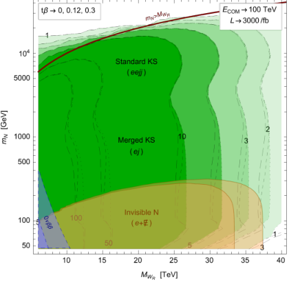
FIG. 10 also shows the impact of the presence of . For , we see a depletion of the observed signal rate, as discussed in section II.3. On the other hand, the production via opens up below and leads to an increase. However, this happens in the light regime, where decay is progressively displaced. Therefore, the dependence on would be of major interest in future studies of displaced decays at FCC-hh.
The missing energy signature. For light , the decay length in the lab frame becomes long enough, such that the probability of it decaying outside of the detector becomes sizeable. Experimentally this shows up as a prompt lepton plus missing energy, which is the signature usually assumed in searches for a sequential CMS:2022krd.
For the FCC-hh we assume a conservative detector size of 5 meters and calculate the expected number of those events, where decays entirely outside of the detector, while always remains prompt. The technical details of this analytical calculation are described at the end of Appendix A. To compare with the estimated expected SM backgrounds, we separate the events into bins of transverse mass , as considered in ATLAS:2017jdr and CMS:2022krd, but we rescale the cross-sections to . The background turns out to be dominated by single production and sub-dominant Drell-Yan, and multi-jet components.
The final result is shown as a shaded orange region and covers the lower part of FIG. 10. It demonstrates that in this channel the expected FCC reach extends up to and up to . The sensitivity reach here is thus slightly higher than in the KS and LJ channels, like it already happens at the LHC Nemevsek:2018bbt, but shows a nice complementarity. The invisible channel reach estimate would be slightly reduced in case a much larger detector size will be chosen, but at the advantage of the other channels discussed above. In addition, the possibility of detecting displaced decays, not yet considered at this stage, would boost the sensitivity of KS in the low regime, as it was argued in Nemevsek:2018bbt.
An important point concerns the connection between colliders and neutrinoless double beta decay () in this light regime. There are a couple of new sources for the rate present in the LRSM Mohapatra:1979ia; Mohapatra:1980yp, in addition to the standard light Majorana neutrino exchange. While the standard double weak decay produces two outgoing electrons with left chirality, in the LRSM new diagrams appear with two right or one left and one right-handed outgoing electron. It turns out that the latter opposite chirality process may be the increasingly dominant one for heavier . It is mediated by the exchange of two ’s, or by one plus one . The latter option has a suppressed nuclear matrix element (see Doi:1985dx; Hirsch:1996qw; Vergados:2002pv and Barry:2013xxa for details), one is left with the double exchange that can produce opposite chirality electrons via the LR gauge boson mixing. This contribution is thus driven by the magnitude of .
The sensitivity to experiments is shown in FIG. 11 for a benchmark value of with the calculable11 1 The size of the mixing is predicted in LRSM via the calculable Dirac mass matrix Nemevsek:2012iq; Senjanovic:2016vxw, but might be enhanced in small corners of parameter space Barry:2013xxa. seesaw Dirac mixing . We depict the region where the LRSM can saturate a possible evidence, for the present and future planned sensitivities (GERDA-II, , and LEGEND-1000, ). One can see that the region extends up to the scale of , with light in the (sub)GeV range. For the region extends up to . We also recall that –few GeV is excluded by the requirement that decays fast enough, in order not to spoil the BBN predictions Nemevsek:2011aa; Nemevsek:2012cd, see the gray shading. These come about because the with such mass is produced thermally in the early universe and then becomes long-lived with and therefore spoils the BBN.

Finally, this region of parameter space harbors the possibility of having a (warm) dark matter(DM) candidate. Namely, for very light masses of close to the keV scale, one can satisfy the DM abundance with entropy dilution Bezrukov:2009th; Nemevsek:2012cd. Indeed, it has been argued in Nemevsek:2012cd that using the phase space suppression for the dilutor lifetime and the drop of relativistic degrees of freedom in around the QCD phase transition, an solution for may be attainable. This requires a very light at about keV, in line with constraints from Dwarf spheroidals DiPaolo:2017geq. Without resorting to the shift, a second solution for exists in the range (see FIG. 6 of Nemevsek:2012cd), which goes further up for heavier DM candidates (see also Dror:2020jzy for the heavy scenarios).
Recently, it was argued that the possibility of having a DM candidate is subject to strong constraints from the large scale structure data Nemevsek:2022anh. This happens because the secondary DM production from entropy injection spoils the matter power spectrum with potentially significant impact on the LR scale. The fate of the DM with low remains to be established, but in any case the interplay with future colliders lies precisely in connecting the DM thermal freeze-out to the missing energy signal at the FCC-hh.
Thus, on FIG. 11 one can appreciate the interplay between and the invisible channel at FCC: a positive finding, in absence of the standard contribution (e.g. because of normal hierarchy, see the discussion in Dvali:2023snt) would imply an upper bound on Nemevsek:2011aa that we estimate in the range of . This would constitute a case for looking for and at an FCC-hh. Further experiments at the kton scale are envisaged to push the search down to an impressive Avasthi:2021lgy. These would connect to LRSM scales as high as , even beyond the reach of a 100 TeV collider.
VI Outlook
While the quest for a theory of neutrino masses is still open, the LRSM stands as a unique candidate connecting their origin with an understanding of parity breaking in weak interactions. Ongoing experimental efforts are at the limit of their capabilities in probing the model parameter space. This is true for collider LHC probes, with an estimated reach of Nemevsek:2018bbt, and also low energy probes. Most notable are current and planned -meson flavour observables that will be sensitive to mass scales at most up to Bertolini:2014sua. It is thus important to address the prospects with the planned and proposed future experiments, with the energy frontier being the elected arena where to search for direct signs of new physics. In this work we systematically estimated the reach of a hadronic () FCC with 100 TeV center of mass energy in the search for a decaying leptonically, which has the potential to uncover lepton number violation, for diverse choices of and , and took into account the LR gauge boson mixing.
We recalled the different signatures emerging as a function of the mass of the RH neutrino : from
i) in the KS process for , to ii) in
case the decay products are merged in a single fat jet for few,
to iii) the signature when decays outside the detector, for .
All these channels feature at least one prompt high lepton, which ensures triggering and allows in reducing
the expected SM background by many orders of magnitude.
It turns out that by requiring a minimal of the order of 1.5 TeV, the background is dominated by w+jets
and could be simulated to satisfactory high statistics.
We showed indeed that, as expected, the background and signal live in different regions of kinematic observables,
thus effectively leaving just the signal at high energies.
As a result, the reach is mainly limited by the center of mass energy, luminosity and by quark PDFs.
We thus assessed the exclusion reach by adopting a unified binned likelihood approach Nemevsek:2018bbt, which does not require sliding windows as a function of model parameter choices. The results were presented in FIG. 10. For the KS and merged regions, i) and ii), we estimated a reach for as high as 35 TeV at 3 C.L., for an integrated luminosity of ab. This is similar to the reach expected for the simpler channel.
It is worth recalling here that within region ii), in the lightest regime of –, the RH neutrino can decay at an appreciable distance, giving rise to a displaced jet Nemevsek:2018bbt. Its study will be very interesting as soon as definite detector geometry and sensitivities become available.
Still, this case overlaps with the even lower regime (case iii) where decays outside the detector and appears as missing energy, thus matching with the search for . We estimated that the sensitivity covers a region extending up to and up to .
This region features an interesting connection with contributions from the LRSM, especially in the light of current, planned and envisioned experiments. FIG. 11 reports this interplay, showing that a possible signal at forthcoming and future probes, in the absence of standard neutrino mass mechanism, would imply a below and below , which overlaps precisely with the invisible decay at FCC here considered. Incidentally, cosmology presents an interesting interplay, either as a constraint from BBN or as an opportunity for having a warm DM candidate.
Acknowledgments
MN is supported by the Slovenian Research Agency under the research core funding No. P1-0035 and in part by the research grants J1-3013, N1-0253 and J1-4389.
Appendix A Drell-Yan and production and decay rates
In this appendix we review in detail the production of and its decays into the final state (on shell and ).
A.1 Resonance production
The amplitude for the production of an on-shell resonance at parton level is
| (10) |
Averaging over initial spins, including the color factor and summing over polarizations , we have
| (11) |
where . The differential cross-section is
| (12) |
such that integration over the final state momentum gives
| (13) |
For the cross-section, we substitute , and obtain
| (14) |
Approximating the function with the Breit-Wigner resonance
| (15) |
we get the parton level cross-section
| (16) |
Proton-proton. To obtain the cross-section, the partonic is convoluted with the PDFs. There is an additional combinatorial factor for the color connection
| (17) |
To integrate over , we change integration variables from to the rapidity of and the partonic center of mass energy . The proton mass is small and quarks are nearly massless, therefore
| (18) |
Moreover, proton beams are symmetric and energetic, such that the momentum is
| (19) |
This setup gives the rapidity
| (20) |
When is produced at rest, we have , which implies and . The product of and is fixed by the on-shell condition for , which gives . Now the maximum value of corresponds to and the maximal rapidity is
| (21) |
This also corresponds to the situation when is maximally boosted
| (22) |
where the last approximation is valid when . Because quarks and protons are nearly massless, the have symmetric limits and . We change variables using the Jacobian
| (23) |
and finally end up with
| (24) |
Both partonic fractions are given by the collision energy and rapidity . The distributions in are symmetric at the LHC and extend to .
A.2 Resonance Decays
The on-shell resonance can decay in different ways. The dominant decay rates are
| (25) | ||||
| (26) |
where , CKM is unitary and . Once we turn on the gauge boson mixing in (1), the decay modes of and , as well as the SM decays to , open up. They proceed with the following rates:
| (27) | ||||
| (28) |
At the same time the dominant rates in (25) and (26) get negligibly suppressed by .
A.3 fermion pair production via resonance
Instead of the resonance production above, we can consider the direct scattering of via the propagator. The scattering amplitude in the unitary gauge is given by
| (29) |
where the momentum part of the propagator vanishes, because we take quarks to be massless. Turning on the gauge boson mixing does not modify the production much, the term goes into . After squaring the amplitude and summing over the spins, we get , because the R and L terms sum into the same expression, moreover the RL interference term vanishes in the limit of zero quark masses. The spin averaged amplitude is
| (30) | ||||
| (31) |
where . The partonic cross-section is then
| (32) | ||||
| (33) | ||||
| (34) |
In the narrow-width limit and expanding near the pole , the cross-section becomes
| (35) | ||||
| (36) |
Proton-proton. The partonic cross-section in (32) is convoluted with the PDFs. The differential cross-section is
| (37) | ||||
and we integrate over the to get the total cross-section
| (38) |
The final state kinematic variables and constrain the integration regions. Let
| (39) | ||||||
| (40) |
where the transverse mass is defined by . At high momentum transfers considered here, the proton and charged lepton masses are negligible and . However, we treat the heavy Majorana neutrino as massive with a mass . From these, we get the and the Mandelstam invariants, and , to be
| (41) |
where . The and rapidities are functions of ( if fixed) and
| (42) | ||||||||
| (43) |
where we introduced
| (44) |
The variable is useful because it corresponds to the invariant mass of the pair, namely . These variables simplify the imposition of cuts and efficiencies. From the matrix element in (30) and the definition of the cross-section in (32), we have
| (45) |
Invariant mass. The . Taking into account that , we get that
| (46) | ||||
| (47) | ||||
where and the Jacobian from is equal to .
Transverse momentum. Along the same lines, the distribution is obtained by the chain rule
| (48) | ||||
| (49) | ||||
| (50) |
This gives us the distribution over , shown in Fig. 3. For , the argument of the square root in (50) needs to be positive, which leads to an upper bound on
| (51) |
Furthermore, at a fixed value of , the lower bound for is given by
| (52) |
and the integration limits in (48) are given by
| (53) |
Invariant mass vs . Likewise, we can get the double differential distribution over and by combining the two chain rules and integrating over
| (54) |
using (45), (49) and (50), where again and . From (49) we see that
| (55) |
The contours of the double differential cross-section are interesting in that they are dominated by a narrow diagonal line relative to off-shell production, and a some broader regions with lower but fixed , corresponding to on-shell .
- No cuts
-
Without cuts, the lower bound on is simply , as needed to produce a massive . However, the integration limits for are split into two regions
(56) Meanwhile, .
- cut
-
can be implemented within the integration limits. Note that does not depend on . From the equation in (43), we have
(57) and from the positivity of the square root, a -independent constant lower bound
(58) appears. The integration plane is , when and for .
- cut
-
restriction makes the limit dependent. Notice that , so setting
(59) while the interval comes from , and , such that
(60) Finally, the bound on coming from (43) is
(61) - and
-
With both cuts acting simultaneously, the integration limits become more complex. The upper bound on remains the same, however the lower bound depends on both, and cuts. More importantly, the interval changes as well as the limits on .
Let us start with the lower bound on . Solving the quadratic equation for in (43) and plugging into , we have
(62) The applies to regions of above (below) 1, where the upper bound is , such that
(63) (64) The lower bound in (62) should not go below the independent one in (58), which happens at
(65) Notice that above a limiting cut
(66) the cut becomes ineffective (we are back to the cut case above) and (66) implies an upper limit on .
as missing energy. Let us compute the number of events , when decays outside of the detector of size . Events are distributed by an exponential distribution
| (67) |
and the total number of events is obtained by integrating from to
| (68) |
where is the total luminosity and is the charged lepton selection efficiency. Efficiencies may also include more stringent and cuts.
References
- (1) J. C. Pati and A. Salam, “Lepton Number as the Fourth Color”, Phys. Rev. D10 (1974) 275–289. [Erratum: Phys. Rev.D11,703(1975)].
- (2) R. N. Mohapatra and J. C. Pati, “Left-Right Gauge Symmetry and an Isoconjugate Model of CP Violation”, Phys. Rev. D11 (1975) 566–571.
- (3) G. Senjanović and R. N. Mohapatra, “Exact Left-Right Symmetry and Spontaneous Violation of Parity”, Phys. Rev. D12 (1975) 1502.
- (4) G. Senjanović, “Spontaneous Breakdown of Parity in a Class of Gauge Theories”, Nucl. Phys. B153 (1979) 334–364.
- (5) P. Minkowski, “ at a Rate of One Out of Muon Decays?”, Phys. Lett. 67B (1977) 421–428.
- (6) R. N. Mohapatra and G. Senjanović, “Neutrino Mass and Spontaneous Parity Nonconservation”, Phys. Rev. Lett. 44 (1980) 912. [,231(1979)].
- (7) T. Yanagida, “Proceedings: Workshop on the Unified Theories and the Baryon Number in the Universe: Tsukuba, Japan, February 13-14, 1979”,.
- (8) S. L. Glashow, “The Future of Elementary Particle Physics”, NATO Sci. Ser. B 61 (1980) 687.
- (9) M. Gell-Mann, P. Ramond, and R. Slansky, “Complex Spinors and Unified Theories”, Conf. Proc. C 790927 (1979) 315–321, arXiv:1306.4669 [hep-th].
- (10) W.-Y. Keung and G. Senjanović, “Majorana Neutrinos and the Production of the Right-handed Charged Gauge Boson”, Phys. Rev. Lett. 50 (1983) 1427.
- (11) Y. Cai, T. Han, T. Li, and R. Ruiz, “Lepton Number Violation: Seesaw Models and Their Collider Tests”, Front. in Phys. 6 (2018) 40, arXiv:1711.02180 [hep-ph].
- (12) A. Ferrari, J. Collot, M.-L. Andrieux, B. Belhorma, P. de Saintignon, J.-Y. Hostachy, P. Martin, and M. Wielers, “Sensitivity study for new gauge bosons and right-handed Majorana neutrinos in collisions at = 14-TeV”, Phys. Rev. D 62 (2000) 013001.
- (13) M. Nemevšek, F. Nesti, G. Senjanović, and Y. Zhang, “First Limits on Left-Right Symmetry Scale from LHC Data”, Phys. Rev. D 83 (2011) 115014, arXiv:1103.1627 [hep-ph].
- (14) J. Gluza, T. Jelinski, and R. Szafron, “Lepton number violation and ‘Diracness’ of massive neutrinos composed of Majorana states”, Phys. Rev. D 93 no. 11, (2016) 113017, arXiv:1604.01388 [hep-ph].
- (15) M. Mitra, R. Ruiz, D. J. Scott, and M. Spannowsky, “Neutrino Jets from High-Mass Gauge Bosons in TeV-Scale Left-Right Symmetric Models”, Phys. Rev. D 94 no. 9, (2016) 095016, arXiv:1607.03504 [hep-ph].
- (16) ATLAS, M. Aaboud et al., “Search for heavy Majorana or Dirac neutrinos and right-handed gauge bosons in final states with two charged leptons and two jets at TeV with the ATLAS detector”, JHEP 01 (2019) 016, arXiv:1809.11105 [hep-ex].
- (17) CMS, A. Tumasyan et al., “Search for a right-handed W boson and a heavy neutrino in proton-proton collisions at = 13 TeV”, JHEP 04 (2022) 047, arXiv:2112.03949 [hep-ex].
- (18) ATLAS, G. Aad et al., “Search for heavy Majorana or Dirac neutrinos and right-handed gauge bosons in final states with charged leptons and jets in collisions at TeV with the ATLAS detector”, arXiv:2304.09553 [hep-ex].
- (19) ATLAS, M. Aaboud et al., “Search for a right-handed gauge boson decaying into a high-momentum heavy neutrino and a charged lepton in collisions with the ATLAS detector at TeV”, Phys. Lett. B 798 (2019) 134942, arXiv:1904.12679 [hep-ex].
- (20) CMS, A. Tumasyan et al., “Search for new physics in the lepton plus missing transverse momentum final state in proton-proton collisions at 13 TeV”, JHEP 07 (2022) 067, arXiv:2202.06075 [hep-ex].
- (21) ATLAS, G. Aad et al., “Search for new resonances in mass distributions of jet pairs using 139 fb-1 of collisions at TeV with the ATLAS detector”, JHEP 03 (2020) 145, arXiv:1910.08447 [hep-ex].
- (22) CMS, A. M. Sirunyan et al., “Search for high mass dijet resonances with a new background prediction method in proton-proton collisions at 13 TeV”, JHEP 05 (2020) 033, arXiv:1911.03947 [hep-ex].
- (23) ATLAS, “Search for vector boson resonances decaying to a top quark and a bottom quark in the hadronic final state using collisions at TeV with the ATLAS detector”,.
- (24) CMS, “Search for W’ bosons decaying to a top and a bottom quark in leptonic final states at ”,.
- (25) CMS, “Search for new heavy resonances decaying to WW, WZ, ZZ, WH, or ZH boson pairs in the all-jets final state in proton-proton collisions at = 13 TeV”, arXiv:2210.00043 [hep-ex].
- (26) M. Nemevšek, F. Nesti, and G. Popara, “Keung-Senjanović process at the LHC: From lepton number violation to displaced vertices to invisible decays”, Phys. Rev. D97 no. 11, (2018) 115018, arXiv:1801.05813 [hep-ph].
- (27) G. Beall, M. Bander, and A. Soni, “Constraint on the Mass Scale of a Left-Right Symmetric Electroweak Theory from the K(L) K(S) Mass Difference”, Phys. Rev. Lett. 48 (1982) 848.
- (28) G. Senjanović and P. Senjanović, “Suppression of Higgs Strangeness Changing Neutral Currents in a Class of Gauge Theories”, Phys. Rev. D21 (1980) 3253.
- (29) G. Ecker and W. Grimus, “CP Violation and Left-Right Symmetry”, Nucl. Phys. B258 (1985) 328–360.
- (30) R. N. Mohapatra, G. Senjanovic, and M. D. Tran, “Strangeness Changing Processes and the Limit on the Right-handed Gauge Boson Mass”, Phys. Rev. D 28 (1983) 546.
- (31) Y. Zhang, H. An, X. Ji, and R. N. Mohapatra, “Right-handed quark mixings in minimal left-right symmetric model with general CP violation”, Phys. Rev. D 76 (2007) 091301, arXiv:0704.1662 [hep-ph].
- (32) A. Maiezza, M. Nemevšek, F. Nesti, and G. Senjanović, “Left-Right Symmetry at LHC”, Phys. Rev. D82 (2010) 055022, arXiv:1005.5160 [hep-ph].
- (33) S. Bertolini, J. O. Eeg, A. Maiezza, and F. Nesti, “New physics in from gluomagnetic contributions and limits on Left-Right symmetry”, Phys. Rev. D86 (2012) 095013, arXiv:1206.0668 [hep-ph]. [Erratum: Phys. Rev.D93,no.7,079903(2016)].
- (34) S. Bertolini, A. Maiezza, and F. Nesti, “Present and Future K and B Meson Mixing Constraints on TeV Scale Left-Right Symmetry”, Phys. Rev. D89 no. 9, (2014) 095028, arXiv:1403.7112 [hep-ph].
- (35) A. Maiezza, M. Nemevšek, and F. Nesti, “Perturbativity and mass scales in the minimal left-right symmetric model”, Phys. Rev. D94 no. 3, (2016) 035008, arXiv:1603.00360 [hep-ph].
- (36) A. Maiezza, G. Senjanović, and J. C. Vasquez, “Higgs sector of the minimal left-right symmetric theory”, Phys. Rev. D95 no. 9, (2017) 095004, arXiv:1612.09146 [hep-ph].
- (37) A. Maiezza and M. Nemevšek, “Strong P invariance, neutron electric dipole moment, and minimal left-right parity at LHC”, Phys. Rev. D90 no. 9, (2014) 095002, arXiv:1407.3678 [hep-ph].
- (38) S. Bertolini, A. Maiezza, and F. Nesti, “Kaon CP violation and neutron EDM in the minimal left-right symmetric model”, Phys. Rev. D 101 no. 3, (2020) 035036, arXiv:1911.09472 [hep-ph].
- (39) A. Maiezza and F. Nesti, “Parity from gauge symmetry”, Eur. Phys. J. C 82 no. 5, (2022) 491, arXiv:2111.11076 [hep-th].
- (40) S. Bertolini, L. Di Luzio, and F. Nesti, “Axion-mediated forces, CP violation and left-right interactions”, Phys. Rev. Lett. 126 no. 8, (2021) 081801, arXiv:2006.12508 [hep-ph].
- (41) T. G. Rizzo, “Exploring new gauge bosons at a 100 TeV collider”, Phys. Rev. D 89 no. 9, (2014) 095022, arXiv:1403.5465 [hep-ph].
- (42) J. N. Ng, A. de la Puente, and B. W.-P. Pan, “Search for Heavy Right-Handed Neutrinos at the LHC and Beyond in the Same-Sign Same-Flavor Leptons Final State”, JHEP 12 (2015) 172, arXiv:1505.01934 [hep-ph].
- (43) P. S. B. Dev, D. Kim, and R. N. Mohapatra, “Disambiguating Seesaw Models using Invariant Mass Variables at Hadron Colliders”, JHEP 01 (2016) 118, arXiv:1510.04328 [hep-ph].
- (44) R. N. Mohapatra, G. Yan, and Y. Zhang, “Ameliorating Higgs induced flavor constraints on TeV scale ”, Nucl. Phys. B 948 (2019) 114764, arXiv:1902.08601 [hep-ph].
- (45) X. Cid Vidal et al., “Report from Working Group 3: Beyond the Standard Model physics at the HL-LHC and HE-LHC”, CERN Yellow Rep. Monogr. 7 (2019) 585–865, arXiv:1812.07831 [hep-ph].
- (46) R. Ruiz, “Lepton Number Violation at Colliders from Kinematically Inaccessible Gauge Bosons”, Eur. Phys. J. C77 no. 6, (2017) 375, arXiv:1703.04669 [hep-ph].
- (47) M. Nemevšek, G. Senjanović, and V. Tello, “Connecting Dirac and Majorana Neutrino Mass Matrices in the Minimal Left-Right Symmetric Model”, Phys. Rev. Lett. 110 no. 15, (2013) 151802, arXiv:1211.2837 [hep-ph].
- (48) G. Senjanović and V. Tello, “Probing Seesaw with Parity Restoration”, Phys. Rev. Lett. 119 no. 20, (2017) 201803, arXiv:1612.05503 [hep-ph].
- (49) G. Senjanović and V. Tello, “Disentangling the seesaw mechanism in the minimal left-right symmetric model”, Phys. Rev. D100 no. 11, (2019) 115031, arXiv:1812.03790 [hep-ph].
- (50) J. Kiers, K. Kiers, A. Szynkman, and T. Tarutina, “Disentangling the seesaw mechanism in the left-right model: An algorithm for the general case”, Phys. Rev. D 107 no. 7, (2023) 075001, arXiv:2212.14837 [hep-ph].
- (51) V. Tello, M. Nemevšek, F. Nesti, G. Senjanović, and F. Vissani, “Left-Right Symmetry: from LHC to Neutrinoless Double Beta Decay”, Phys. Rev. Lett. 106 (2011) 151801, arXiv:1011.3522 [hep-ph].
- (52) J. Barry and W. Rodejohann, “Lepton number and flavour violation in TeV-scale left-right symmetric theories with large left-right mixing”, JHEP 09 (2013) 153, arXiv:1303.6324 [hep-ph].
- (53) F. Bezrukov, H. Hettmansperger, and M. Lindner, “keV sterile neutrino Dark Matter in gauge extensions of the Standard Model”, Phys. Rev. D 81 (2010) 085032, arXiv:0912.4415 [hep-ph].
- (54) M. Nemevšek, G. Senjanović, and Y. Zhang, “Warm Dark Matter in Low Scale Left-Right Theory”, JCAP 07 (2012) 006, arXiv:1205.0844 [hep-ph].
- (55) M. Nemevšek and Y. Zhang, “Dark Matter Dilution Mechanism through the Lens of Large-Scale Structure”, Phys. Rev. Lett. 130 no. 12, (2023) 121002, arXiv:2206.11293 [hep-ph].
- (56) G. Barenboim, K. Huitu, J. Maalampi, and M. Raidal, “Constraints on doubly charged Higgs interactions at linear collider”, Phys. Lett. B 394 (1997) 132–138, arXiv:hep-ph/9611362.
- (57) K. Huitu, J. Maalampi, A. Pietila, and M. Raidal, “Doubly charged Higgs at LHC”, Nucl. Phys. B 487 (1997) 27–42, arXiv:hep-ph/9606311.
- (58) J. Maalampi and N. Romanenko, “Single production of doubly charged Higgs bosons at hadron colliders”, Phys. Lett. B 532 (2002) 202–208, arXiv:hep-ph/0201196.
- (59) A. Roitgrund and G. Eilam, “Search for like-sign dileptons plus two jets signal in the framework of the manifest left-right symmetric model”, JHEP 01 (2021) 031, arXiv:1704.07772 [hep-ph]. [Erratum: JHEP 03, 029 (2021)].
- (60) A. Maiezza, M. Nemevšek, and F. Nesti, “Lepton Number Violation in Higgs Decay at LHC”, Phys. Rev. Lett. 115 (2015) 081802, arXiv:1503.06834 [hep-ph].
- (61) M. Nemevšek, F. Nesti, and J. C. Vasquez, “Majorana Higgses at colliders”, JHEP 04 (2017) 114, arXiv:1612.06840 [hep-ph].
- (62) J. Alwall, P. Demin, S. de Visscher, R. Frederix, M. Herquet, F. Maltoni, T. Plehn, D. L. Rainwater, and T. Stelzer, “MadGraph/MadEvent v4: The New Web Generation”, JHEP 09 (2007) 028, arXiv:0706.2334 [hep-ph].
- (63) T. Sjostrand, S. Mrenna, and P. Z. Skands, “A Brief Introduction to PYTHIA 8.1”, Comput. Phys. Commun. 178 (2008) 852–867, arXiv:0710.3820 [hep-ph].
- (64) DELPHES 3, J. de Favereau, C. Delaere, P. Demin, A. Giammanco, V. Lemaître, A. Mertens, and M. Selvaggi, “DELPHES 3, A modular framework for fast simulation of a generic collider experiment”, JHEP 02 (2014) 057, arXiv:1307.6346 [hep-ex].
- (65) FCC-hh Collaboration, M. Selvaggi et al., “Official Delphes card prepared by FCC-hh collaboration”, Dec, 2017. https://hep-fcc.github.io/FCCSW/.
- (66) M. L. Mangano et al., “Physics at a 100 TeV pp Collider: Standard Model Processes”, arXiv:1607.01831 [hep-ph].
- (67) M. Nemevšek and F. Nesti, “LRSM FeynRules model file, version 1.7”, 2020. https://sites.google.com/site/leftrighthep/1-lrsm-feynrules.
- (68) A. Roitgrund, G. Eilam, and S. Bar-Shalom, “Implementation of the left-right symmetric model in FeynRules”, Comput. Phys. Commun. 203 (2016) 18–44, arXiv:1401.3345 [hep-ph].
- (69) ATLAS, A. collab., “Search for a new heavy gauge boson resonance decaying into a lepton and missing transverse momentum in 36 fb-1 of collisions at TeV with the ATLAS experiment”, ATLAS-CONF-2017-016 (4, 2017) .
- (70) R. N. Mohapatra and G. Senjanović, “Neutrino Masses and Mixings in Gauge Models with Spontaneous Parity Violation”, Phys. Rev. D23 (1981) 165.
- (71) M. Doi, T. Kotani, and E. Takasugi, “Double beta Decay and Majorana Neutrino”, Prog. Theor. Phys. Suppl. 83 (1985) 1.
- (72) M. Hirsch, H. V. Klapdor-Kleingrothaus, and O. Panella, “Double beta decay in left-right symmetric models”, Phys. Lett. B 374 (1996) 7–12, arXiv:hep-ph/9602306.
- (73) J. D. Vergados, “The Neutrinoless double beta decay from a modern perspective”, Phys. Rept. 361 (2002) 1–56, arXiv:hep-ph/0209347.
- (74) M. Nemevšek, F. Nesti, G. Senjanović, and V. Tello, “Neutrinoless Double Beta Decay: Low Left-Right Symmetry Scale?”, arXiv:1112.3061 [hep-ph].
- (75) C. Di Paolo, F. Nesti, and F. L. Villante, “Phase space mass bound for fermionic dark matter from dwarf spheroidal galaxies”, Mon. Not. Roy. Astron. Soc. 475 no. 4, (2018) 5385–5397, arXiv:1704.06644 [astro-ph.GA].
- (76) J. A. Dror, D. Dunsky, L. J. Hall, and K. Harigaya, “Sterile Neutrino Dark Matter in Left-Right Theories”, JHEP 07 (2020) 168, arXiv:2004.09511 [hep-ph].
- (77) G. Dvali, A. Maiezza, G. Senjanović, and V. Tello, “Neutrinoless double beta decay as seen by the devil’s advocate”, arXiv:2303.17261 [hep-ph].
- (78) A. Avasthi et al., “Kiloton-scale xenon detectors for neutrinoless double beta decay and other new physics searches”, Phys. Rev. D 104 no. 11, (2021) 112007, arXiv:2110.01537 [physics.ins-det].