Chemodynamical models of our Galaxy
Abstract
A chemodynamical model of our galaxy is fitted to data from DR17 of the APOGEE survey supplemented with data from the StarHorse catalogue and Gaia DR3. Dynamically, the model is defined by action-based distribution functions for dark matter and six stellar components plus a gas disc. The gravitational potential jointly generated by the model’s components is used to examine the galaxy’s chemical composition within action space. The observational data probably cover all parts of action space that are populated by stars. The overwhelming majority of stars have angular momentum implying that they were born in the Galactic disc. High- stars dominate in a region that is sharply bounded by . Chemically the model is defined by giving each stellar component a Gaussian distribution in ([Fe/H],[Mg/Fe]) space about a mean that is a linear function of the actions. The model’s 47 dynamical parameters are chosen to maximise the likelihood of the data given the model in 72 three-dimensional velocity spaces while its 70 chemical parameters are similarly chosen in five-dimensional chemo-dynamical space. The circular speed falls steadily from at to at . Dark matter contributes half the radial force on the Sun and has local density , there being in dark matter and in stars within of the plane.
Keywords:
The Galaxy, Galaxy: kinematics and dynamics – The Galaxy, Galaxy: abundances – The Galaxy, Galaxy: disc – The Galaxy, Galaxy: fundamental parameters – The Galaxy, Galaxy: structure1 Introduction
ESA’s Gaia satellite provides locations and space velocities for tens of millions of stars (Gaia Collaboration et al. 2021; Gaia Collaboration et al. 2022). In anticipation of the arrival of Gaia astrometry, several teams around the world have been accumulating the spectra of millions of stars at higher resolution than Gaia can achieve and using these spectra to derive the stars’ chemical compositions, which are expected to yield insight into our Galaxy’s history. The APOGEE survey (Majewski et al. 2017) is particularly powerful in this respect because, being based on the mid-infrared H band, it can probe the disc nearer the plane and over a wider radial range than other surveys, which are more strongly restricted by dust.
Since the middle of the 20th century we have known that the ages and chemical compositions of stars vary systematically with their locations and velocities (Roman 1950; Roman 1999; Eggen et al. 1962; Gilmore & Wyse 1998; Fuhrmann 2011). With the emergence of the theory of nucleosynthesis (Burbidge et al. 1957) and models of the chemical evolution of the ISM (Tinsley 1980; Pagel 1997) conviction grew that by studying the chemodynamical structure of our Galaxy we should be able to trace its history (Freeman & Bland-Hawthorn 2002). Over the last two decades efforts to realise this goal have taken two lines of attack. One line centres on simulations of galaxy formation that include gas, stars and dark matter, usually in some sort of cosmological context (Brook et al. 2004; Grand et al. 2017, e.g.). Another line of attack models the Galaxy as a series of annuli within which stars form from gas that they simultaneously enrich (Matteucci & Francois 1989; Chiappini et al. 1997; Schönrich & Binney 2009a; Schönrich & McMillan 2017; Sharma et al. 2021; Chen et al. 2022). Strengths of the latter line of attack include the ability to fit models to the very detailed data now available for our Galaxy and to develop understanding of how specific physical processes, such as radial migration and the late arrival of type Ia supernovae manifest themselves in observational data.
The central premise of Schönrich & Binney 2009a and much prior work is that all disc stars were born on nearly circular orbits in the plane from gas that is azimuthally well mixed, so its metallicity [Fe/H] and -abundance [Mg/Fe] are functions of Galactocentric radius and look-back time . Since the gross chemistry of stellar atmospheres evolves little, to a good approximation it then follows that the location ([Fe/H],[Mg/Fe]) of a star in the chemical plane is an (a priori unknown) function of its birth radius and age. SB09 modelled the functions [Fe/H] and [Mg/Fe] by adopting a radial profile of star formation and following the production of heavy elements and the dispersal of these elements by radial flows and winds. This effort lead to predictions for the number and chemistry of stars born at each radius and time.
Fluctuations in the Galaxy’s gravitational potential cause the orbits of stars to drift (Binney & Lacey 1988, e.g.). Sellwood & Binney 2002 divided this drift into (i) ‘blurring’, which is the drift away from circular orbits to more eccentric and inclined orbits, and (ii) ‘churning’, by which stars change their angular momenta without increasing their random velocities. By adjusting the intensity of blurring and churning, SB09 were able to match the distribution of solar-neighbourhood stars in chemical space. Remarkably, the observed bimodality of the chemical distribution emerged naturally in a model in which the star-formation rate declined monotonically with time and radius. The bimodality was a consequence of the rapid decline in [Mg/Fe] about a gigayear after the start of star formation as type Ia supernova set in.
The methodology of SB09 has been extended in various directions. Chen et al. 2022 updated their work by (a) using recent nucleosynthetic yields, and (b) comparing the model predictions at 24 locations in the Galaxy rather than just in the solar neighbourhood. This important latter step was made possible by DR14 of the APOGEE survey. Sharma et al. 2021 had previously fitted models to these data but instead of deriving chemical compositions from a model of star formation and nucleosynthetic yields, they specified a functional form for [Fe/H] that contains parameters to be fitted to the data. They further assumed that [Mg/Fe] is a function of [Fe/H] and age that has a specified functional form, and fitted the form’s parameters to the data.
Both Sharma et al. 2021 and Chen et al. 2022 followed SB09 in adopting a Schwarzschild DF (e.g. Binney & Tremaine 2008, §4.4.3). Several powerful arguments favour use of DFs that are functions of the action integrals rather than the approximate energies and (Binney & McMillan 2016, e.g.), so Sanders & Binney 2015 reformulated SB09 in terms of action-based DFs. Specifically, they assumed that in the absence of churning, the DF of each coeval cohort of disc stars would have the form of the quasi-isothermal DF that was introduced by Binney & McMillan 2011. Blurring was represented by the radial and vertical velocity dispersion parameters of the DF being functions of age, and the cohort’s current DF was obtained by convolution of this quasi-isothermal DF with a kernel that represented diffusion in . Unfortunately at that time model-data comparisons were only possible in the solar neighbourhood, but the work of Sharma et al. 2021, in which a model was successfully fitted to the wide-ranging APOGEE data, is methodologically similar to Sanders & Binney 2015.
These studies approach the data with a clear preconception of our Galaxy’s history. Our aim here is to be more data-driven: regardless of history, how are the Galaxy’s stars distributed in ‘chemodynamical space’ – the five-dimensional space spanned by the actions, [Fe/H] and [Mg/Fe]? Logically this question should precedes the question of why stars are distributed as they are. A map of this distribution would be an invaluable descriptor of our Galaxy that would transcend theories of galaxy formation.
Binney & Vasiliev 2023 used the AGAMA software package (Vasiliev 2019) to fit to Gaia DR2 data a model in which both stars and dark matter were represented by DFs of the form and moved in the potential that they and interstellar gas jointly generate. Here we revise and extend this model: we revise it by modelling the Galaxy’s bulge as a fat disc rather than a spheroid; we update it by fitting to data from APOGEE and the third rather than the second Gaia data release, and we extend it by assigning a chemical model to each of its stellar components.
In Section 2 we describe the stellar sample that we have analysed. Section 3 first examines how the means of [Mg/Fe] and [Fe/H] vary with location in action space and then studies the stellar density and mean values of the actions in four regions of action space within which particular stellar components are expected to dominate. Section 4 introduces a scheme for modelling the Galaxy’s chemodynamical structure: Section 4.1 explains how we extend a model based on standard DFs to a chemodynamical model; Section 4.2 defines the functional forms we have assumed for ; Sections 4.3 to 4.6 specify the values of the model parameters from which data-fitting commenced, explain our strategy for dealing with the survey’s selection function, and define the likelihood that the search maximises and the maximising procedure. Section 5 describes the model fitted to the data and discusses the quality of the fit it provides. Section 6 compares the scope of the present model to that of the widely used Besançon model, and Section 7 sums up and identifies next steps. Appendix A validates our procedure for maximising a likelihood.
2 The data
From the 17th data release of the Sloan Digital Sky Survey (Abdurro’uf et al. 2022) we selected data for stars that have Gaia DR3 astrometry (Gaia Collaboration et al. 2021; Gaia Collaboration et al. 2022) and parameters from the StarHorse catalogue (Queiroz et al. 2018; Anders et al. 2022; Queiroz et al. 2023). We removed stars with a probability of belonging to a globular cluster according to Vasiliev & Baumgardt 2021, stars with the STAR_WARN bit (7) of the ASPCAP_FLAG set, and stars with a StarHorse distance with an uncertainty larger than . We further required the astrometric ‘fidelity’ parameter of Rybizki et al. 2022 to exceed . Finally, the sample was restricted to giants by requiring and . We convert heliocentric data to galactocentric coordinates assuming the Sun’s phase-space coordinates are (GRAVITY Collaboration et al. 2022) and (Schönrich 2012; Reid & Brunthaler 2020).
Fig. 1 shows the spatial distribution of the sample’s stars projected onto the plane and planes in the upper and lower panels, respectively. The upper panel shows very clearly the rapid variation of the selection function inevitable in a pencil-beam spectroscopic survey. Also evident is the strong bias towards the Sun inevitable in a magnitude-limited survey. Notwithstanding these regrettable characteristics, the figure shows that the survey provides good coverage of the Sun’s side of the Galaxy below in the radial range .


3 Action-space chemistry
We computed the giants’ phase-space coordinates and from them computed the actions , and in the gravitational potential of the self-consistent Galaxy model that is presented in Section 5 below. In this potential stars are bound and 97 unbound; actions cannot be computed for unbound stars, so these stars were eliminated from the sample.
3.1 Mean values of [Fe/H] and [Mg/H]
The panels of Fig. 2 show the mean value of [Mg/Fe] in cells in action space, while Fig. 3 shows mean values of [Fe/H]. The left columns show projections onto the plane grouped by their values of , while the right columns show projections onto the plane grouped by values of . In the left columns the values of increase from the bottom panel upwards, while in the right columns the values of increase upwards – the relevant range in or is shown at top-right of each panel.
Stars on orbits that are either nearly circular or in the plane contribute, respectively, to the bottom left or right pair of panels in each figure, while stars on orbits that are either highly eccentric or highly inclined contribute to the top pair of panels.
Fig. 4 shows the number of stars contributing to the bottom and top left panels of Figs. 2 and 3. These numbers are strongly influenced by APOGEE’s selection function. In particular, the lower panel for low shows a strong concentration around the Sun’s location. The plots of mean [Mg/Fe] and [Fe/H] in Figs. 2 and 3 show no sign of this bias.
Note the extraordinarily wide coverage in – at low there are stars with down to zero from a maximum value that exceeds twice the Sun’s value of (). This wide coverage of at small is possible because APOGEE extends to low Galactic latitude and covers an unprecedentedly wide range in Galactic radius , so it includes stars on near circular orbits at a wide range of radii.
In every panel of Figs. 2 to 4 the populated region has a sharp left edge that lies just to the left of the line . If stars were in fact strictly confined to , observational errors would still cause some stars to scatter to . Indeed, a small over-estimation of the distance to a star at and can move a star from the near to the far side of the Galactic centre without much effect on its apparent velocity, and thus reverse the sign of its measured . The sharpness of the left boundaries of the populated regions in Figs. 2 to 4 attest to the accuracy of the StarHorse distances used to compute .
The near total confinement of stars to is a clear indication that the overwhelming majority of stars were born in a disc within our Galaxy – stars accreted from other galaxies would end up on orbits with both signs of with roughly equal probability. A significant part of the stellar halo is thought to comprise such accreted stars, and as a consequence the halo shows negligible net rotation. The stellar halo should be dominant at small and significant and/or . Hence the sharpness of the boundary at in all the panels of Figs. 2 to 4 implies that the stellar halo contributes rather few stars to the sample. It may well be that halo stars, being metal-poor and thus weak-lined, have trouble passing our spectroscopic quality cuts. Moreover, our requirement that a star’s distance uncertainty should not exceed will have removed many distant halo stars. A better requirement might be upper limits on the uncertainties in and because what really matters is the fractional uncertainties in and not the absolute uncertainty in distance.
There are several remarkable features of Fig. 2:
- •
Along the axis of the bottom left panel of Fig. 2 there is a narrow orange region indicative of solar [Mg/Fe]. This is the low- disc. Above it a blue-shaded region of high [Mg/Fe] fills the interior of a U centred on . To left and right as well as below, this region transitions sharply to yellow shades indicative of lower [Mg/Fe]. The blue region is part of the high- disc.
- •
In this bottom-left panel, to the right of yellow shades extend to the highest populated values of . This phenomenon clearly shows that low- stars, even ones on significantly inclined orbits, dominate at . It implies that the high- disc has a remarkably sharp outer edge at roughly .
- •
As one proceeds up the left column of Fig. 2 through samples of stars with increasing , the orange/yellow region of the thin, low- disc yields ground to the blue high- region. This phenomenon indicates that the high- disc extends down to ; at low it is overwhelmed by the low- disc, but comes to the fore as increases because its DF decreases less rapidly with increasing .
- •
Similar trends are evident as one proceeds up the right column of Fig. 2 through samples of stars with increasing , except that in the range the yellow shades of low- stars recede more rapidly: in fact they have already disappeared from the sample with . This phenomenon indicates that the main body of the low- disc covers a wider range in than in , as is natural in a ‘thin’ disc.
- •
The V of green colours that pushes down at in the bottom right panel of Fig. 2 suggests that within the low- disc has a minimum just interior to the Sun.
- •
Whereas in the bottom left panel of Fig. 2 brown shades are confined to a narrow band above the axis, in the bottom-right panel at they extend to . This indicates that the outer low- disc is radially hot.
- •
In the top two panels of the right column of Fig. 2, blue colours indicative of high- extend right down to the axis except at very low and . This indicates that at the high- disc dominates outside the bulge and the outer disc.
Fig. 3 shows mean values of [Fe/H] in the format used to display [Mg/Fe] in Fig. 2. Blue shades now imply low metallicity, so the high- disc with is coloured cyan, wile the metal-rich, inner low- disc is coloured yellow. With this colour scheme very similar patterns are observed in Fig. 3 to those discussed above for Fig. 2: high- often implies low-metallicity. The most striking difference occurs in the region : in Fig. 3 this region is largely green because the outer low- disc is metal poor. However in the bottom right panel of Fig. 3 a tongue of yellow is evident at that signals that the low- disc becomes radially excited before it turns metal-poor.
The bottom-left panel of Fig. 3 (for ) shows [Fe/H is confined to small except at small . The bottom-right panel shows that at small and , [Fe/H occurs predominantly at large . These facts are consistent with the idea that metal-rich stars populate the kind of tightly bound, eccentric, low-inclination orbits that form the backbone of the bar. In the bottom right panel of Fig. 3 (for ) in the range a yellow-brown ridge reaches upwards: this is the signature of a vertically thin annulus of fairly metal-rich stars on eccentric orbits.
Figs. 2 and 3 bear comparison with Fig. 31 of Gaia Collaboration et al. 2023, which shows the distribution of more than 5 million stars in the plane. The chemistry of these stars was determined from Gaia radial velocity spectra, and in four of its panels, cells are coloured by median [M/H] or median [/Fe]. The left panels plot over a wide range in while the right panels zoom into the most densely populated part of the plane : and . One of the zoomed panels shows steep drops in [M/Fe] along two lines that slope up and to the left, intersecting the axis at and . One of these features is probably related to the drop apparent in the lower-right panels of Fig 3 but the correspondence is not clear. The bottom-right panel of the figure in the Gaia paper shows a decline in [/Fe] around , but again the line of steepest descent slopes up and to the left rather than running straight up, and it isn’t as sharp as that seen in Fig. 2 (and in Fig. 20 below). In this connection, note that the Gaia paper tracks [/Fe] through lines of calcium rather than magnesium.


3.2 The ([Fe/H], [Mg/Fe]) plane
Figs. 2 and 3 show just mean values of [Mg/Fe] and [Fe/H]. To gain further insight we now explore distributions in the ([Fe/H],[Mg/Fe]) plane for the four regions of the plane that are marked in Fig. 5 over a plot of the standard deviation in [Mg/Fe] in the slice of action space with smallest . The standard deviation tends to be large where components with differing chemistry overlap.
The first of these regions, labelled A, lies along the axis at and . Stars in this region are on highly inclined orbits, so they dominate the stellar density near the axis. We call this the bulge/halo region. The second region, B, occupies the heart of the high- region of action-space – and . The third region, labelled C, lies just above the axis at . Stars in this region are on nearly planar orbits, so will be predominantly thin-disc stars. The fourth region, D, at , is dominated by the outer, flaring disc.
The contours in Fig. 6 show the chemical structure of these four regions: the bulge/halo, high- disc, thin-disc and outer disc regions are depicted by rows from top to bottom. In the left, centre and right columns the colours show mean values of , and , respectively. It should be borne in mind that the stellar densities contoured, unlike the mean values plotted in Fig. 2, reflect the APOGEE selection function. Most significantly, stars near the Sun are over-represented.
- •
The top row of Fig. 6 shows that the bulge/halo region is indeed a superposition of two components, one centred on ([Fe/H],[Mg/Fe] and the other on ([Fe/H],[Mg/Fe]. The first population has a tail that extends to [Fe/H at slightly lower [Mg/Fe]. It is probably a mixture of the high- disc and the stellar halo with the former dominating. The metal-rich, low- component is presumably the bulge. The mean values of and shown by the colours vary little with chemistry, although there is a marginal tendency for to decrease with [Fe/H] and to be negative at [Fe/H]. The central panel shows that increases systematically with decreasing [Fe/H]. That is, is lowest in the bulge, highest in the halo and intermediate in the high- disc.
- •
The second row in Fig. 6 shows the chemistry of the high- region. The dominant component is centred on ([Fe/H],[Mg/Fe], with a tail sloping down to solar chemistry (0,0) and beyond. Within the dominant, high- component, the left panel shows that any gradient in is weak, although at [Fe/H] there is a slight tendency for to decrease with [Fe/H]. The central panel shows a systematic increase in with decreasing [Fe/H] within the high- component but no evidence of an analogous gradient in the low- component.
- •
The thin-disc region shown in the third row of Fig. 6 comprises a dominant component centred on ([Fe/H],[Mg/Fe] that must be the main body of the low- disc. On top we see a significant tail from the high- disc. Thus the high- disc makes a significant contribution to the thin-disc region. The right panel of the third row shows that in the dominant component, increases with [Mg/Fe] – this is likely the signature of stochastic heating: stars with larger [Mg/Fe] are older and kinematically hotter. Another effect of age increasing with [Mg/Fe] is the widening spread in [Fe/H] with increasing [Mg/Fe]: older stars have migrated further with the consequence that in the over-represented solar-neighbourhood group an older population displays a wider spread in [Fe/H]. The colours in the left panel of the third row indicate that the dominant component has a clear gradient in , which must be a manifestation of the familiar metallicity gradient in the disc (e.g. Méndez-Delgado et al. 2022, and references therin). There is no sign of an analogous gradient in the high- component. Surprisingly, the third row shows a tendency for to increase with [Mg/Fe] – given that stars contributing to this row have by construction , it is puzzling to observe significant variation of . The signal is unmistakable nonetheless. Stars with exceptionally low must lie very close to the plane, so they are either very close to the Sun or are significantly extincted. Could high extinction artificially lower their measured values of [Mg/Fe]?
Taken together the second and third rows confirm the presence of two populations that coexist at many points in action space. The low- population dominates at low and the high- population dominates at high .
The first and second rows show that stars metal-poorer than are only encountered at [Mg/Fe. Moreover, these stars are confined to and .
- •
The bottom panels of Fig. 6 show the chemistry of the outer, flaring disc. It is almost entirely accounted for by a single population centred on ([Fe/H],[Mg/Fe]. This low- population shows the gradient in that we encountered in the inner low- disc, so we have every reason to suppose that this population is just an extension of the dominant component in the third row (the low- disc). Moreover, the central and right panels of the fourth row show the same trends in and we encountered in the third row, and attributed to increasing age and stochastic heating with [Mg/Fe].
Perhaps the most striking aspects of Fig. 6 are two ‘dogs that didn’t bark’: (i) the absence of stars at low-metallicity and low- in the top row (bulge/halo region) and (ii) the complete disappearance of the high- population between the second and fourth rows (high- and outer disc regions). Another notable result is the contrast between the strong gradients in , and in the low- disc and the extremely weak gradients in mean actions in the high- component.
Fig. 7 reveals key differences in how low- and high- stars are distributed in action space by plotting projections of the sample onto the plane in the upper, and the plane in the lower, pairs of panels. The absence of high- stars at is striking, as is the extent to which the low- stars extend to high at both small and large while being restricted to lower at intermediate . In , the pattern of the low- stars is very different: the populated region reaches highest in at intermediate even though stars with large can reach the Sun, and thus boost their chances of entering the sample, only if they have large . The wide spread in at may be the result of resonant scattering by spirals, while the wide spread in at large might be a legacy of tidal interactions with objects in the dark halo.
It is worth noting how much the bottom panel of Fig. 7 differs from similar plots of stellar density in the plane for stars near the Sun (Hunt et al. 2019; Trick et al. 2019, e.g.): here we see no lines associated with resonances. To see these features, the sample must be restricted to a narrow band in radius or distance from the Sun because (as Fig. 7 demonstrates) resonant orbits are not more- or less-populated than neighbouring non-resonant orbits. They nonetheless appear to be so if we impose a sufficient selection in angle variables ` because resonant terms in the Hamiltonian shuffle stars between the actions that are the axes of the plots. This motion is correlated with `, so at some angles the density of stars has been enhanced at particular actions, while at other angles the density at these actions has been diminished. A sample that is strongly selected in radius or distance from the Sun is biased in both and and thus reveals the effects of perturbing terms in a way that the broadly selected sample of Fig. 7 does not.
The sample of stars with high-quality RVS spectra analysed by Gaia Collaboration et al. 2023 covers quite a wide range in and distance from the Sun but it is much more concentrated around the Sun that the APOGEE sample. This may be why it shows ridges in the . As the Gaia paper remarks, it is not evident that its ridges are the same as those presented by Hunt et al. 2019 and Trick et al. 2019. The ridges of the Gaia paper are most evident in its plot of median values of , the greatest distance a star moves from the plane. Fig. 8 is a plot of the mean value of that ought to be closely related to a plot of mean values of . Any ridges analogous to those in the Gaia paper are extremely indistinct.
4 Modelling the data
We now turn to the construction of a chemodynamical model of our Galaxy that reproduces as closely as possible the trends discovered in the last section.
4.1 EDF structure
Sanders & Binney 2015 introduced the concept of an extended distribution function (EDF), that is a density of stars in the five-dimensional space spanned by and chemistry,
| (1) |
An excellent way of summarising the chemodynamical structure of our Galaxy would be to decompose it into components that individually have simple EDFs. Specifically, we seek components that have analytic dynamical DFs that are extended to EDFs by multiplication by an analytic probability density that gives the probability that a star with actions has the chemistry . Any EDF can be written as a product – simply define and and is trivial to show that – but we want to define our components so is analytic.
Non-negativity is a fundamental property of a probability density function (pdf), and multi-Gaussian expansions are widely used to approximate non-negative functions analytically. In this spirit we assume that can be approximated by a Gaussian distribution in with mean and dispersion depending on .
The general Gaussian two-dimensional probability density can be written
| (2) |
where is a symmetric matrix and the subscripts imply dependence on – in order to limit the number of parameters to determine, we assume that is independent of . A simple assumption is that depends linearly on :
| (3) |
where is a two-component object and is a matrix. Without loss of generality, we can choose the reference actions to be similar to those of the Sun, with the implication that becomes the mean chemistry of stars in the given component that are on solar-type orbits.


4.2 DFs of the components
We follow BV23 in modelling the stellar component of our Galaxy with six DFs . Five of these are instances of a generalisation of the exponential DF introduced by Vasiliev 2019. The overall DF is a product of factors
| (4) |
The function controls the breadth of the distribution in and thus the velocity dispersions and near the equatorial plane. The function similarly controls the breadth of the distribution in and hence controls both the thickness of the disc and the velocity dispersion . The other three factors control the disc’s radial profile. On its own, the factor generates a roughly exponentially declining surface density . The factor tapers this profile towards the centre. At a theoretical level, this factor is motivated by the notion that the central portion of the disc has morphed into the bar/bulge leaving a depression at the centre of the surviving disc. At an empirical level, modelling the young disc through the observed distribution of OB stars, Li & Binney 2022 concluded that an exponential that extends right to the centre predicts too many stars at small radii. The factor truncates the disc at some outer radius. This feature is motivated by the sharp transition from blue to yellow at in Fig. 2, which suggests that the high- disc has a sharp outer edge. These factors take the form
| (5) |
where
| (6) |
Here the action determines the characteristic radius of the central depression and is a parameter that determines the sharpness of its boundary. Similarly, the action determines the disc’s outer truncation radius and sets the sharpness of the cutoff there. If is set to a negative value, is returned, ensuring that there is no central depression or radial truncation.
The functional forms adopted for and are essentially the same as those adopted by BV23:
| (7) |
where
| (8) |
Here is the action that sets the disc’s characteristic scale length and the action sets the velocity dispersions and . The exponent controls the radial variation of these dispersions: the larger is, the faster the dispersions fall with radius. The action , a surrogate for energy, is taken to be
| (9) |
where is a constant that controls the way the dispersions vary at small radii as discussed by BV23. The factor has the form
| (10) |
where
| (11) |
with a constant that controls the way the surface density varies at small radii, as discussed by BV23. These formulae for , and are the same as those in BV23 except that here and depend on and in addition to . Since disc stars typically have the additional dependence of and is generally insignificant. It does, however, yield more plausible velocity distributions in the neighbourhood of .
We follow BV23 in modelling the low- disc as a superposition of three discs, presumed to be of increasing age and velocity dispersion: the young, middle-aged and old discs. Away from their centres, these discs are simple exponentials, but they may have central depressions in their surface density consistent with the bar/bulge having formed out of them. BV23 modelled the bulge by a spheroidal DF. Figs. 2, 3 and 7 indicate that this was a poor choice by suggesting that the bulge is almost entirely confined to , as is natural in a component that formed from a thin disc. Therefore we model the bulge as a truncated exponential, in which is small and and are large.
The high- disc is assumed to be a radially truncated exponential. The stellar halo is modelled by the same non-rotating spheroidal DF used by BV23. This probably provides a poor representation of the truth, but since the halo contributes very little to the APOGEE data, we defer improvement of its DF to future work.
4.3 Initial parameters
The chemodynamical model we are fitting has a large number of parameters. An automated search for a good model through a high-dimensional space is unlikely to succeed if started from a random location. Hence we started by hand-fitting the DFs to the dynamical data in the manner described by BV23. The resulting model differed from that of BV23 principally because the data employed extended from to rather than the narrower range .
The starting parameters of the DFs were largely taken to be those determined by BV23. Experiment showed that central tapers in the surface densities of disc components tend to yield circular-speed curves that rise more slowly than the data imply, so in the final model only the young disc has a central taper. For the high- disc, the sharp colour transition in Fig. 2 around motivated the choice , .
| Component | |||||||||||
|---|---|---|---|---|---|---|---|---|---|---|---|
| young disk | |||||||||||
| middle disk | |||||||||||
| old disk | |||||||||||
| high- disk | |||||||||||
| stellar halo | |||||||||||
| bulge |
The other fresh choices required for the DFs were all the parameters of the bulge’s DF. The bar/bulge extends out to , which corresponds to , so should be a value of this order; we started from and . The bulge is a hot component, so we started from and .
Table 1 lists the initial values of the chemical parameters. On the left we have the tilt of the Gaussian ellipsoids with respect to the chemical axes11 1 The angle is defined such the , where and . and the means and dispersions of those Gaussians at the Sun’s action-space location. As we proceed from young disc to old and high-, the mean value of [Fe/H] is presumed to decline while that of [Mg/Fe] is presumed to increase. The dispersions and increase along this sequence consistent with the evidence that stars diffuse from circular orbits as they age. The bulge is assumed to be metal-rich and -normal, with a large dispersion .
The gradients of chemistry in action space are listed on the right of Table 1. Most values are set to zero. Exceptions are the coefficients that set the radial metallicity gradients in the thin disc and the stellar halo – these are set to a value similar to that, per Mpc, that was inferred for d[Fe/H]/d by Spina et al. 2022 for open clusters. Other non-zero values are of and for the old disc; these imply that [Mg/Fe] increases with eccentricity and inclination, and a value for the high- disc’s that implies strongly decreasing [Fe/H] with inclination.
4.4 Managing the APOGEE selection function
As remarked above, the contours in Fig. 6 depend on APOGEE’s very complex, dust-dependent, selection function (SF) in addition to the EDF. Our approach to circumventing this problem is as follows. Our basic assumption is that the SF is independent of both velocity and chemistry but depends strongly on position. The independence of velocity is clear; less so is the independence of since colour criteria were involved in the selection of stars. Nonetheless any dependence of the SF on must be tiny by comparison with the dependence on .
Since our model is axisymmetric and symmetric in , velocity distributions are functions of only. So we bin the real stars in the 72 bins in space that are specified by Table 222 2 It is strictly neither necessary nor desirable to bin the real stars in space – we could sample velocity space at the location of each real star, but that would be computationally expensive. Grouping stars into bins merely reduces the computational cost of generating mock stars, and our goal in choosing bins is to cover real space as evenly as possible with the smallest number of bins. and determine the barycentre of the stars in the th bin – let be the number of stars in this bin. Then, given a trial set of components and their EDFs, we determine the density contributed by the th component at and let
| (12) |
be times the fraction of real stars predicted to be contributed by the th component. Now we create mock stars by sampling velocity space at under the velocity distribution specified by . Each chosen velocity corresponds to an action , and we use this to choose a chemistry by sampling the Gaussian . When this is done, each spatial bin contains mock stars in addition to the real stars. The mock stars, unlike the real stars, have known component memberships.
BV23 should perhaps have stressed the novelty of their approach to mapping a galaxy’s gravitational field. Competing methods, using the Jeans equations (Read & Steger 2017, e.g.) or Schwarzschild modelling (van den Bosch et al. 2008; Zhu et al. 2018, e.g), hinge on knowledge of the density of a stellar component. BV23 predict the densities of components, but they they use as an input only the density profile in the solar cylinder. The basic physical principle of the BV23 approach is most easily understood in the context of a one-dimensional problem. Let be the system’s phase-space coordinates and let with , so is the bottom of the potential well. Then at stars of every energy are present, and at we find only stars with . Moreover, the velocity distribution in the vicinity of at location follows from the shape of the velocity distribution in the vicinity of at . In words: the potential relates velocity distributions at different locations, so it’s logically possible to recover it from those velocity distributions without knowing the stellar density . When the DF is isothermsl, , the velocity distribution, , is the same Gaussian at all locations and cannot be recovered without knowing . Fortunately, no stellar system can have an isothermal DF because the latter includes many unbound stars.
4.5 Defining the likelihood
Given a model potential , a set of DFs and a model chemistry, we compute the log likelihood of the data as follows. We distribute each bin’s mock stars over a grid in velocity space by the cloud-in-cell algorithm (e.g. Binney & Tremaine 2008, Box 2.4). The velocity grid has cells covering the cuboid with boundaries at , and to , where , , and . Here the grid size is proportional to the cube root of the number of real stars and etc are the standard deviations of the components of the velocities of the real stars: ranged up to 23 with average value .
The mass assigned to each grid cell is then divided by the number of mock stars in the relevant spatial bin. Then we use the cloud-in-cell algorithm to determine the mock-star density at the location of each real star and compute the contribution of the th spatial bin to the overall dynamical log likelihood as the sum over stars of the logarithms of these densities. In Appendix A we show that the maximum value of under variation of the masses assigned to cells, subject to a fixed total mass on the grid, is achieved when the mass of mock stars in each cell coincides with the mass that would be obtained by distributing the real stars over the grid in the same way that the mock stars are distributed.
The dynamical log likelihood is the sum
| (13) |
over spatial bins normalised by the number of real stars. This normalisation prevents the likelihood being dominated by grid cells that lie close to the Sun and are in consequence heavily populated: sparsely populated cells far from the Sun are powerful probes of the Galaxy’s structure.
| 0 | 0.3 | 0.7 | 1 | 1.5 | 2 | 3 | |||||||
|---|---|---|---|---|---|---|---|---|---|---|---|---|---|
| 0.5 | 1.5 | 3 | 4 | 5 | 6 | 7 | 8 | 9 | 10 | 11.5 | 13 | 14.5 |
The computation of the chemical contribution to the log likelihood is similar. We use the cloud-in-cell algorithm to distribute the mock stars over a five-dimensional grid . Then the mass assigned to each cell is divided by the number of mock stars, and is computed as the mean of the logarithm of the grid density at the location of each real star. The final log likelihood is
| (14) |
An indication of how closely a model approximates the data can be obtained by distributing real rather than mock stars over the grids and then computing as before by determining the grid density at the locations of the real stars. We call this the perfect-fit value of . The perfect-fit and actual-fit values of for the chosen model are and , while the corresponding values of are and .
We will see below that the algorithm chooses surprisingly large values for some dispersions and gradient coefficients . We tested the robustness of thee choices by including in the quantity to be maximised a Gaussian prior term proportional to and/or . These priors had little effect.
4.5.1 A shortcut
The procedure just described assumes that the mock stars are drawn from the current DFs. It is expedient to be able to compute from mock stars obtained by sampling a DF that differs slightly from the current DF, . To do this we weight each mock star by , the ratio of the star’s current probability density to the probability density when it was randomly drawn. The sum of these weights is the number of ‘effective’ mock stars and this is the number used to normalise the masses in cells after distributing mock stars on a grid. The need to re-sample was determined by monitoring the largest values of . There is no need to re-sample after varying the chemical model.
4.6 Likelihood maximisation
We have used the Nelder-Mead algorithm encapsulated in the agama function findMinNdim to minimise . We alternated a few hundred steps in which the chemical model was fixed while the DFs were varied with a few hundred steps in which the DFs were fixed and the chemical model was varied. The code sought to maximise the sum of and regardless of which parameters were being varied because is useful when changing the DFs: it is sensitive to the relative masses of components and indicates whether a deficiency of stars at some phase-space location should be remedied by increasing the mass of the high- disc or the old disc, for example.
When the DFs are varied without updating the potential , the fit quality is invariant under multiplication of the masses of every component’s DF by a common factor: with fixed, the fit depends only on the relative masses of components. So the Nelder-Mead algorithm varied the DFs with the total stellar mass held constant.
After a few hundred Nelder-Mead adjustments of the DFs, the DF parameters were reviewed and potentially changed by hand before updating to self-consistency. Then a new sample of mock stars was drawn.


5 results
Regardless of whether it is the DFs or the chemical model that is being adjusted, the Nelder-Mead algorithm yields a sequence of values that increases rapidly at first and then more and more slowly. So one does not have the impression that it has located a global maximum. Hence the model presented here has the status of fitting the data about as well as any model we have tried rather than being a definitive model.
The full curve in Figs 9 shows the circular-speed curve of the final potential; also shown are the contributions to from the baryons (blue dotted curve) and dark matter (black dashed curve) along with several previous estimates of derived from tracers presumed to be on near-circular (Mróz et al. 2019; Ablimit et al. 2020), and a study of red giants by Eilers et al. 2019. At , where circular orbits are prohibited by the bar, the model curve deviates significantly from the triangular points from Wegg & Gerhard 2013, which describe the axisymmetric component of a non-axisymmetric potential. Clearly we cannot expect an axisymmetric model to reproduce the data for this region, but the extent of the conflict with earlier work suggests that our bulge is too massive and insufficiently compact. At the model curve in Fig. 9 runs just above most of the points from previous studies. This is a consequence of taking for the Sun: when is increased, the black (data) curves in the right columns of Figs. 13 to 15 move to the right and the potential has to be adjusted to make the red (model) curves follow them. Our value for follows directly from the observations of Sgr A* and the assumption that this black hole can define the Galactic rest frame (Reid & Brunthaler 2020; GRAVITY Collaboration et al. 2022). Since the model predicts the Sun’s peculiar velocity is . These values are consistent with the values and reported by Schönrich 2012.
The full curve in Fig. 10 shows the model density of stars as a function of at the solar radius, while the points describe the observational estimates of this by Gilmore & Reid 1983 and Jurić et al. 2008, which can be moved vertically because they relate to star density rather than mass density. The agreement is satisfactory. The black dashed line shows the almost constant density of dark matter, while the blue curves show the density profiles of the young disc (full curve), the middle disc (dotted curve), the old disc (short-dashed curve) and the high- disc (long-dashed curve). The red dotted curve shows the tiny contribution from the stellar halo. The dark halo makes the largest contribution to the density at .
Comparison with Figs 14 and 15 in BV23 shows that the differences between the circular-speed curves of the two models are confined to the bar-bulge region – the curve of the BV23 model rises much more steeply at . The BV23 discs are less massive, yield a shorter overall radial scale length , and have smaller scale heights – this is especially true of the old disc, for which the parameter has jumped from 5 to . At the old and high- discs of BV23 have much lower and significantly lower , changes that are clearly mandated by the new data. The local densities of dark matter are almost identical in the two models.
The full blue curve in Fig. 11 shows the surface density of disc stars as a function of radius while the black dotted curve shows the surface density of all stars. At the surface density falls nearly exponentially with scale length (marked by the red dashed curve). This is a significantly longer scale-length than was inferred by Robin et al. 2003 from the 2MASS survey. Recently, Robin et al. 2022 inferred a scale-length parameter for the DFs of the thin disc components, which is best compared to the values of for the young and middle discs and for the old disc. Bovy et al. 2012 derived scale lengths for mono-abundance populations in APOGEE and found that these increased steadily from to as [Mg/Fe] decreases and [Fe/H] increases. The results in Table 3 are qualitatively consistent with that early work.
The full curve in the upper panel of Fig. 12 shows as a function of radius the density of stars at , while the blue curves show the corresponding densities of the disc components. The contributions of the bulge and the stellar halo are shown by the black and red dotted curves. The density of the dark halo is shown by the black long-dashed curve.
The blue curves in the lower panel of Fig. 12 show the mean streaming velocities at of the three thin-disc components and of the high- disc. Asymmetric drift causes the streaming velocity to fall further and further below the circular speed as the velocity dispersions increase. The black dotted curve shows the rising mean streaming velocity in the bulge.
Tables 3 to 5 list the model’s parameters, while Figs 13 to 18 show the resulting fits to data. These figures show that this model fits many aspects of the data very well while showing shortcomings in other aspects.
5.1 Fits to kinematics
Figs. 13 to 15 show, from left to right in each column, distributions of , and marginalised over the other two velocity components for the 72 spatial bins that were used to compute . In the panels for and the histograms cover where is the standard deviation, while the histograms of cover to . From bottom to top of each column the radius of the spatial bin increases, while different columns correspond to different values of : the numbers at the bottom of each histogram give the mean values of and of stars in the relevant bin. The black histograms show the APOGEE DR17 Gaia DR3 data while the red histograms show the distributions of mock stars.
| Component | ||||||||||||
|---|---|---|---|---|---|---|---|---|---|---|---|---|
| young disk | – | – | ||||||||||
| middle disk | – | – | – | – | ||||||||
| old disk | – | – | – | – | ||||||||
| high- disk | – | – | ||||||||||
| bulge | – | – |
| Component | ||||||||
|---|---|---|---|---|---|---|---|---|
| dark halo | ||||||||
| stellar halo |
The largest discrepancies between data and model occur in at small and (bottom right of each column in Fig. 13). These bins are dominated by the Galactic bar, so it is natural that our axisymmetric model fails to model the data well. More surprising is how well the model fits the and distributions for these bins, and even provides passable fits to the distributions above (lower right of the columns of Figs 14) and 15).
The model generally provides good fits to the histograms at . This result implies that the potential correctly gives the circular speed because, as BV23 explained, even a small mismatch between a model’s circular speed and the true circular speed leads to an unmistakable displacement of the red and black curves in the plots. If some histograms for show discrepancies, it is because the model under-predicts stars with .
In a few of the histograms for and (see the top of Fig. 13) the red model curve fits the black data curve on one side much better than on the other. Since the red curves are by construction left-right symmetric (up to shot noise), such one-sided fits point to deviations from equilibrium in the data caused by spiral structure or tidal interactions, for example (McMillan et al. 2022; Khanna et al. 2023, e.g.).


| Component | |||||||||||
|---|---|---|---|---|---|---|---|---|---|---|---|
| young disk | |||||||||||
| middle disk | |||||||||||
| old disk | |||||||||||
| high- disk | |||||||||||
| stellar halo | |||||||||||
| bulge |
5.1.1 Parameters of the DFs
Tables 3 and 4 give the parameters of the fitted DFs. The middle disc is the most massive disc component: with it is 50 percent more massive than the old and high- discs and nearly three times as massive as the young disc. The bulge with is slightly more massive than the middle disc. The mass, , of the stellar halo is gravitationally negligible. As discussed in Section 3, our sample may be biased against very metal-poor stars, so the mass we report for the stellar halo is likely an underestimate – for the halo within Deason et al. 2019 estimate luminosity leading to mass at least twice our value.
The young and middle discs have comparable scale actions , while the old and high- discs have much smaller scale actions, and , respectively. In the context of inside-out growth of galaxies, this result is to be expected. The parameter values and for the young disc imply that it does not differ strongly from a pure exponential. The high- disc is quite sharply radially truncated near : , .
The scale actions and that control the in-plane and vertical velocity dispersions increase, as expected, along the sequence young disc, middle disc, old disc, high- disc. The biggest jump in occurs between the young and the middle disc, while the biggest jump in occurs between the middle and old disc, so the disc with the largest velocity anisotropy is the middle disc. Such anisotropy is the signature of heating by spiral arms (Binney & Lacey 1988, e.g.).
The value of for the bulge is very similar to that of the high- disc, while the bulge’s value for is only half that of the high- disc.
The values of the parameter that controls the radial gradient of the in-plane velocity dispersions increases systematically along the sequence young – high- disc. This result implies that the radial gradient in steepens along this sequence.
The parameter that controls the radial gradient in does not vary systematically along the disc sequence. The middle disc has the most negative value of and therefore the weakest radial gradient, while the high- disc has the steepest radial gradient.
The bulge DF’s values and ensure that the bulge is compact. Its in-plane dispersions are similar to those of the high- disc () but it has much smaller vertical dispersions and extent because versus for the high- disc. For some reason has been set large and positive (causing to decline steeply with ) while causes to decline much more slowly with . Consequently the bulge is most anisotropic at small radii. The bulge mass, may be compared with the value that Portail et al. 2015 estimated from made-to-measure modelling of data for red-clump giants.
The total stellar mass is , on the lower side of recent estimates. At the stellar density is in the plane falling to at .
At the density of dark matter is in the plane falling to at in agreement with most recent estimates (see Fig. 1 of de Salas & Widmark 2021, for a review). The vertical component of the gravitational acceleration at satisfies
| (15) | ||||
| (16) |
The actual surface density of stars and dark matter within of the plane is slightly lower than the naive estimate based on because the gravitational field has a large, position dependent, radial component. It is
| (17) |
and comprises in stars, in dark matter and in gas.
In Table 4 the mass of the dark halo is given as but the great majority of this mass lies outside the volume for which we have data. The scale radius of the dark halo is set by the parameter , which was arbitrarily set to , so the volume modelled lies inside , where, in the absence of the stars, the dark-matter density would satisfy . As explained by BV23, the actual density profile of the dark halo is more complex on account of the pull of the stars.
5.2 Fits to chemistry
Figs. 16 to 18 show predicted (left panels) and observed distributions in the ([Fe/H],[Mg/Fe]) plane within 30 bins in the plane – the actions at the centre of the bin are given at the bottom of the bin’s model panel. As one proceeds up each column, the mean value of increases, so the bulge or thin disc dominates the bottom panels of each column. As one proceeds from column to column, the mean value of increases, so the typical Galactocentric radius of stars increases from the left column of Fig. 16 to the right column of Fig. 18. Fig. 10 of Eilers et al. 2022 show similar data in a slightly different representation by plotting vertically rather than .
In Fig. 16 the largest discrepancies between data and model occur around . This region of action space will be dominated by the stellar halo and the bulge and we have no confidence in the functional forms we have have adopted for their DFs, so it is not surprising that the model performs least well there. In fact it is encouraging that the model does capture the main features of the chemistry even there: in particular a strongly populated ridge that slopes from ([Fe/H],[Mg/Fe]) up towards , which has conentrations towards each end that vary in importance with .
At and (bottom of the right column of Fig. 16) the model under-populates the principal ridge at high [Fe/H] and low [Mg/Fe].
Fig. 17, which covers , shows good agreement between model and data at all values of except the largest: at the top of he left column the model struggles to reproduce a population of metal-rich, low- stars. This issue with a deficit of metal-rich, low- stars at high is the only significant shortcoming of the fits shown in Fig. 18 for the largest angular momenta. Data for the stars that the model fails to provide is sparse and most liable to observational error, so it is not clear how significant the deficit in the model is.
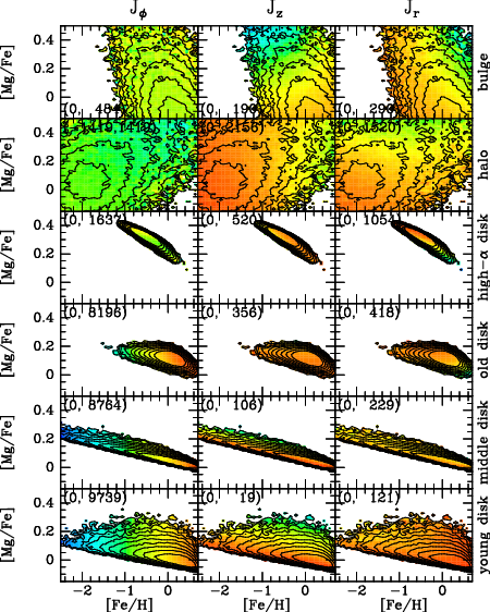
5.2.1 Chemical parameters
Table 5 gives the values of the parameters of the chemical model that yields the fits shown in Figs. 16 to 18, while each row of Fig. 19 displays the chemodynamical structure of the component listed along the figure’s right-hand edge. Contours show the density of stars with a given chemistry that one obtains by sampling the DF without any selection function and then using the chemical model of Table 5 to assign a chemistry to each selected star. This plot differs from all our other plots in being representative of what the model claims is out there, rather than what APOGEE can see. In the left column each pixel is coloured by the mean of the values of the stars in that pixel, while the centre and right columns are coloured by the mean values of and , respectively. The numbers in brackets in each panel show the values (in ) associated with red and blue.
The contours in the top row of Fig. 19 show that the main body of the bulge is modelled as a very metal-rich, roughly -normal structure. From this there extends a tail of stars with progressively higher [Mg/Fe] and slightly lower [Fe/H]. The ridge line is similar to the standard evolutionary trajectory of a population that has a high star-formation rate (Schönrich & Binney 2009b, e.g.). The colours in the top row show that in the bulge chemistry barely depends on but [Mg/H] increases with and [Fe/H] increases with .
The second row in Fig. 19 shows that the stellar halo is modelled as a metal-poor structure () widely scattered over the chemical plane (). Its chemistry depends little on but significantly on and in the sense of [Fe/H] increasing with and [Mg/H] increasing with – the reverse of the dependencies in found the bulge. The stellar halo is now believed to owe much to the ‘Enceladus’ merger event, which formed a mildly counter-rotating, relatively metal-rich, radially anisotropic and flattened component of the halo (Belokurov et al. 2018; Helmi et al. 2018; Myeong et al. 2018). According to this picture the mean value of should increase with [Fe/H] while the mean value of should decrease with [Fe/H]. These are the trends seen in the bulge and not those Fig. 19 implies for the halo.
The third row of Fig. 19 shows that the high- disc covers a narrow range in chemistry, all at large [Mg/H] as we expect of a component that formed before type Ia supernovae became important. The narrowness of its footprint reflects a notably small dispersion , 24 times smaller than its dispersion in . Table 5 shows that [Fe/H] depends only weakly on and in the sense that metallicity increases withe and therefore radius. Schönrich & McMillan 2017 discuss the origin of this ‘inverse metallicity gradient’. [Fe/H] depends quite strongly on and but in opposing directions: increasing with ad decreasing with .
The bottom three rows of Fig. 19, for the thin-disc components, show distributions that slope in the same sense as the bulge and thick disc but more gradually so they do not reach such large values of [Mg/Fe]. In these components the dominant dependence of chemistry on actions is upon and the value given for the middle disc implies , consistent with the values to deduced by Méndez-Delgado et al. 2022 for interstellar N and O, respectively.
The young and middle discs extend to much lower [Fe/H] than the old disc, which is a priori surprising. The reason is that the these discs have lager scale actions so they are predicted to extend to larger radii and higher values of . Given the negative value of , the outer (largely unobserved) parts of these discs are predicted to be very metal-poor. It is likely that diminishes for much larger than the solar value, with the consequence that does not fall to the low values predicted under our assumption of constant .
The middle, old and high- discs have implying that metallicity increases with eccentricity. Radial migration, combined with radial gradients in metallicity and can generate this correlation: at a given value of there are stars that migrated outwards and inwards. On average, the former will have higher metallicities and radial actions than the latter, thus inducing a correlation between metallicity and at given . In the young disc, by contrast, [Fe/H] decreases with .
The chemistry of the young disc depends strongly on and very strongly on . In part this may reflect the smaller range in actions within this cool component. Fig. 19 shows that [Mg/H] increases strongly with and decreases with . The young disc’s value of is small so significant values of [Mg/H] are reached when is abnormally large. This fact accounts for the sharp lower boundary of the thin disc’s footprint in the bottom panels of Fig. 19.
All thin-disc components have , implying an outward increase in [Mg/Fe], while for the high- discs . Thus the signs of both and reverse as one passes to the high- disc from the thin disc. Given that high [Mg/Fe] is the signature of a high star-formation rate, it is natural for to be negative in the absence of radial migration.
The discs’ values of decrease along the young – old sequence so [Mg/Fe] increases with eccentricity in the young disc and decreases with eccentricity in the old and high- discs. is positive but decreasing along the young – high- sequence. A picture in which [Mg/Fe] increases with age and stars are secularly scattered away from planar, circular orbits implies that [Mg/Fe] should increase with eccentricity and inclination. Table 5 shows that it does increase with inclination but in the older components it is flat or decreasing with eccentricity.
The left columns of Figs 2 and 3 show the mean values of observed [Mg/Fe] and [Fe/H] split into tranches of . The right panels of Fig. 20 show the same data but regardless of . The U-shaped boundary to the (blue) region dominated by the high- disc is now spectacularly evident, and in the lower plot the metal-rich thin disc is seen to be bounded below by and above by , interestingly coinciding with the right-hand boundary of high- disc.
The left panels of Fig. 20 show the model’s version of these plots. The principal features are captured but the match is far from perfect. Most notably, in the upper left plot the boundary of the U-shaped region is insufficiently sharp and [Mg/H] is too low at . In the lower left plot [Fe/H] is too high at low and .


6 Comparison with the Besançon model
A natural question is how the present model compares with the ‘Besançon Galaxy model’ (BGM), which has recently been updated by Robin et al. 2022 to self-consistency in the context of Gaia DR3 astrometry. Major differences include: (i) In the BGM the bulge, the stellar halo and the dark halo were represented by pre-defined density distributions rather than DFs. The BGM bulge is spherical while the two haloes are ellipsoidal; (ii) In the BGM the integrals used are rather than ; (iii) The BGM was fitted to sky-plane velocities computed using inverse parallaxes rather than StarHorse distances, and line-of-sight velocities were not used; (iv) The BGM was fitted to (a) the distributions of stars within of the Sun viewed in 36 directions, and (b) the and parallax distributions of more distant stars viewed along 26 lines of sight. Fits were made to the and quantiles in and rather than to densities in three-dimensional velocity space at 72 locations in . (v) Rather than ignoring age distributions as we have done, the BGM embodies them by being fitted to colour-magnitude diagrams at various locations; (vi) Modelling the parallax distributions required engagement with the Gaia scanning law, and adoption of both a dust model and a luminosity functions for each DF. (vi) The Galaxy’s circular-speed curve was an input to the BGM model whereas here it follows from the fits to the kinematics.
While there are significant differences in the data employed and how the model parameters were fitted, the two models have similar scope: both are axisymmetric, self-consistent dynamical models from which mock samples can be drawn by specifying selection criteria. The present model does not come with pre-defined luminosity functions but the new version of agama provides for each DF to include a luminosity function appropriate to the component’s age and chemistry. The new version defines classes for lines of sight and dust models, so magnitude-limited samples can be drawn for any line of sight.
7 Conclusions
The APOGEE spectroscopic survey combined with Gaia astrometry casts a brilliant light on the chemodynamical structure of our Galaxy. From DR17 of the Sloan Digital Sky Survey we selected just under 218 000 giant stars that are unlikely to belong to globular clusters and have reliable distances in the Bayesian StarHorse catalogue (Anders et al. 2022). The selected stars cover the radial range and lie within of the plane.
We have avoided engaging with the complex selection function of the APOGEE survey by examining the kinematic and chemical distributions within 72 spatial bins that extend from to at .
We have used these distributions to update and extend the self-consistent dynamical model of BV23. This model is defined by distribution functions for six stellar components and the dark halo, together with a prescribed surface density of gas. The gravitational potential that these eight ingredients jointly generate was computed iteratively and the resulting predictions for the kinematics of stars at 72 spatial locations were compared with the data.
The functional forms adopted for the DFs differ from those used by BV23. A major difference is that here the bulge is assumed to be a fat disc rather than a spheroidal component. Another difference is that here the high- disc is taken to be radially truncated. A minor difference is in the way the variables and introduced by Vasiliev 2019 are defined.
Another difference with BV23 is in how the kinematic data are fitted: whereas BV23 fitted by hand histograms of , and marginalised over the other two components of velocity, we have used the Nelder-Mead algorithm to fit the predicted densities of stars in 72 three-dimensional velocity spaces.
In a major extension of BV23 we have added a chemical dimension to the model by assigning to each stellar DF a probability density in the chemical space . These probability densities are Gaussians with mean values that are linear functions of .
We examined the variation in action space of the mean values of [Mg/Fe] and [Fe/H]. Plots of this distribution (Figs. 2 and 20) show a sharp boundary at that is a testament to the accuracy of the StarHorse distances we have used. It also implies that within the (wide) spatial region covered by the data, few bulge stars counter-rotate, so the bulge should not be modelled as a spheroidal component but as a hot disc. In addition to the sharp boundary at , plots of show a sharp transition at that we interpret as radial truncation of the high- disc.
Devising a mathematical formula for the density of objects in a five-dimensional space is challenging. We have broken the task into dynamical and chemical parts. We consider that the dynamical problem has been satisfactorily solved as regards disc stars, but less satisfactorily as regards the bulge and the spheroidal components. Given a DF, one has to quantify the density of its stars in chemical space, which the data show to be a function of actions: is the only gradient coefficient conventionally considered, but Table 5 shows that it is by no means the only significant coefficient, even bearing in mind that spans a wider range than the other two actions. The simplest ansatz for a probability density is a Gaussian, but the Gaussian’s properties must be continuous functions of the actions. We have implemented the simplest, non-trivial scheme, namely similar Gaussians centred on means that depend linearly on the actions. Even though this scheme is very basic, we ended up needing 70 parameters for the chemical pdf.
Alternatively, we could have followed Sanders & Binney 2015 and used a model inspired by the notion that disc stars diffuse from circular orbits. We were discouraged from pursuing this idea by unsuccessful attempts to model the APOGEE data published in Hayden et al. 2015 by the approach of Sanders & Binney 2015, but the proposal might be worth revisiting. A radically different scheme would be to represent the logarithm of the star density as a sum of basis functions, such as wavelets. A successful scheme would combine flexibility, a low parameter count and intrinsic non-negativity. Given the very basic nature of our ansatz, the fits to data shown in Figs. 16 to 18 may be counted a success.
We followed BV23 in representing the age distribution in the thin disc with three distinct discs, rather than following Binney 2012 and Sanders & Binney 2015 in using a single thin-disc DF that includes an age parameter. Given the limited success of the discrete approach, a return to continuous variation with age may be wise. The challenge is to model in a flexible yet parameter-poor way the dependence upon age of both the dynamical and the chemical parameters.
It is likely that the replacement of the halo and bulge DFs by better functional forms would make it possible to obtain better fits even without restructuring the chemical model. DFs that are not confined to one sign of are subject to subtle constraints, as will be explained elsewhere (Binney in preparation). The parameters of the functional form used for the stellar and dark-matter DFs cannot be freely varied if unphysical kinematics are to be avoided, with the consequence that in the model neither component is as radially biased as it probably should be. The data imply that the bulge like the discs lies overwhelmingly at but its DF should surely not vanish completely at , as it does in the model. This artificial vanishing of the bulge DF may be responsible for the poor match of the model’s circular-speed curve to the points from Wegg & Gerhard 2013 in Fig. 9. Including in the modelling some observational bias against low-metallicity stars may also improve fits.
Our ‘to do’ list is as follows: (i) replace the quality cut on distances by cuts based on uncertainties in and , and possibly relax quality cuts on low-metallicity stars in order to reduce biases against halo stars; (ii) replace the DFs of dark and stellar haloes and explore more anisotropic DFs for these components; (iii) try to replace the three thin-disc DFs by a single DF that includes age-dependent dynamics and chemistry; (iv) add age data.
A model such as ours can be used to make innumerable predictions regarding orbits around the Galaxy and the density of stars of given chemistry at any location in phase-space; here we have shown only a tiny selection of such predictions. For example, it would be interesting to produce plots like Fig. 10 of Eilers et al. 2022 or to fit the functional forms of Lian et al. 2022 to the spatial structures of our low- and high- discs and compare with the values Lian et al obtained. Using the agama package it is easy to make predictions in seconds by drawing from the model samples of stars with known component memberships. In addition to yielding mock observations, such samples can be used as initial conditions for an N-body simulation. Vasiliev 2019 showed that simulations started in this way form precisely equilibrium systems, and subtle departures from equilibrium can be explored by slightly shifting the phase-space coordinated returned by agama before advancing the N-body model in time.
DATA AVAILABILITY
The code that generates Galaxy models and fits the present chemical models can be downloaded from the agama website https://github.com/GalacticDynamics-Oxford/Agama.
References
- Abdurro’uf et al. (2022) Abdurro’uf et al., 2022, ApJS, 259, 35
- Ablimit et al. (2020) Ablimit I., Zhao G., Flynn C., Bird S. A., 2020, ApJL, 895, L12
- Anders et al. (2022) Anders F. et al., 2022, A&A, 658, A91
- Belokurov et al. (2018) Belokurov V., Erkal D., Evans N. W., Koposov S. E., Deason A. J., 2018, MNRAS, 478, 611
- Binney (2012) Binney J., 2012, MNRAS, 426, 1328
- Binney & Lacey (1988) Binney J., Lacey C., 1988, MNRAS, 230, 597
- Binney & McMillan (2011) Binney J., McMillan P. J., 2011, MNRAS, 413, 1889
- Binney & McMillan (2016) Binney J., McMillan P. J., 2016, MNRAS, 456, 1982
- Binney & Tremaine (2008) Binney J., Tremaine S., 2008, Galactic Dynamics: Second Edition. Princeton University Press
- Binney & Vasiliev (2023) Binney J., Vasiliev E., 2023, MNRAS, 520, 1832
- Bovy et al. (2012) Bovy J., Rix H.-W., Liu C., Hogg D. W., Beers T. C., Lee Y. S., 2012, ApJ, 753, 148
- Brook et al. (2004) Brook C. B., Kawata D., Gibson B. K., Freeman K. C., 2004, ApJ, 612, 894
- Burbidge et al. (1957) Burbidge E. M., Burbidge G. R., Fowler W. A., Hoyle F., 1957, Reviews of Modern Physics, 29, 547
- Chen et al. (2022) Chen B., Hayden M. R., Sharma S., Bland-Hawthorn J., Kobayashi C., Karakas A. I., 2022, arXiv e-prints, arXiv:2204.11413
- Chiappini et al. (1997) Chiappini C., Matteucci F., Gratton R., 1997, ApJ, 477, 765
- de Salas & Widmark (2021) de Salas P. F., Widmark A., 2021, Reports on Progress in Physics, 84, 104901
- Deason et al. (2019) Deason A. J., Belokurov V., Sanders J. L., 2019, MNRAS, 490, 3426
- Eggen et al. (1962) Eggen O. J., Lynden-Bell D., Sandage A. R., 1962, ApJ, 136, 748
- Eilers et al. (2019) Eilers A.-C., Hogg D. W., Rix H.-W., Ness M. K., 2019, ApJ, 871, 120
- Eilers et al. (2022) Eilers A.-C., Hogg D. W., Rix H.-W., Ness M. K., Price-Whelan A. M., Mészáros S., Nitschelm C., 2022, ApJ, 928, 23
- Freeman & Bland-Hawthorn (2002) Freeman K., Bland-Hawthorn J., 2002, AnnRA&A, 40, 487
- Fuhrmann (2011) Fuhrmann K., 2011, MNRAS, 414, 2893
- Gaia Collaboration et al. (2021) Gaia Collaboration et al., 2021, A&A, 650, C3
- Gaia Collaboration et al. (2023) Gaia Collaboration et al., 2023, A&A, 674, A38
- Gaia Collaboration et al. (2022) Gaia Collaboration et al., 2022, arXiv e-prints, arXiv:2208.00211
- Gilmore & Reid (1983) Gilmore G., Reid N., 1983, MNRAS, 202, 1025
- Gilmore & Wyse (1998) Gilmore G., Wyse R. F. G., 1998, AJ, 116, 748
- Grand et al. (2017) Grand R. J. J. et al., 2017, MNRAS, 467, 179
- GRAVITY Collaboration et al. (2022) GRAVITY Collaboration et al., 2022, A&A, 657, L12
- Hayden et al. (2015) Hayden M. R. et al., 2015, ApJ, 808, 132
- Helmi et al. (2018) Helmi A., Babusiaux C., Koppelman H. H., Massari D., Veljanoski J., Brown A. G. A., 2018, Nat, 563, 85
- Hunt et al. (2019) Hunt J. A. S., Bub M. W., Bovy J., Mackereth J. T., Trick W. H., Kawata D., 2019, MNRAS, 490, 1026
- Jurić et al. (2008) Jurić M. et al., 2008, ApJ, 673, 864
- Khanna et al. (2023) Khanna S., Sharma S., Bland-Hawthorn J., Hayden M., 2023, MNRAS, 520, 5002
- Li & Binney (2022) Li C., Binney J., 2022, MNRAS, 516, 3454
- Lian et al. (2022) Lian J. et al., 2022, MNRAS, 513, 4130
- Majewski et al. (2017) Majewski S. R. et al., 2017, AJ, 154, 94
- Matteucci & Francois (1989) Matteucci F., Francois P., 1989, MNRAS, 239, 885
- McMillan et al. (2022) McMillan P. J. et al., 2022, MNRAS, 516, 4988
- Méndez-Delgado et al. (2022) Méndez-Delgado J. E., Amayo A., Arellano-Córdova K. Z., Esteban C., García-Rojas J., Carigi L., Delgado-Inglada G., 2022, MNRAS, 510, 4436
- Mróz et al. (2019) Mróz P. et al., 2019, ApJL, 870, L10
- Myeong et al. (2018) Myeong G. C., Evans N. W., Belokurov V., Sanders J. L., Koposov S. E., 2018, ApJL, 856, L26
- Pagel (1997) Pagel B. E. J., 1997, Nucleosynthesis and Chemical Evolution of Galaxies. Cambridge University Press
- Portail et al. (2015) Portail M., Wegg C., Gerhard O., Martinez-Valpuesta I., 2015, MNRAS, 448, 713
- Queiroz et al. (2023) Queiroz A. B. A. et al., 2023, A&A, 673, A155
- Queiroz et al. (2018) Queiroz A. B. A. et al., 2018, MNRAS, 476, 2556
- Read & Steger (2017) Read J. I., Steger P., 2017, MNRAS, 471, 4541
- Reid & Brunthaler (2020) Reid M. J., Brunthaler A., 2020, ApJ, 892, 39
- Robin et al. (2022) Robin A. C. et al., 2022, A&A, 667, A98
- Robin et al. (2003) Robin A. C., Reylé C., Derrière S., Picaud S., 2003, A&A, 409, 523
- Roman (1950) Roman N. G., 1950, ApJ, 112, 554
- Roman (1999) Roman N. G., 1999, Ast. Phys. Sp. Sci., 267, 37
- Rybizki et al. (2022) Rybizki J. et al., 2022, MNRAS, 510, 2597
- Sanders & Binney (2015) Sanders J. L., Binney J., 2015, MNRAS, 449, 3479
- Schönrich (2012) Schönrich R., 2012, MNRAS, 427, 274
- Schönrich & Binney (2009a) Schönrich R., Binney J., 2009a, MNRAS, 396, 203
- Schönrich & Binney (2009b) Schönrich R., Binney J., 2009b, MNRAS, 399, 1145
- Schönrich & McMillan (2017) Schönrich R., McMillan P. J., 2017, MNRAS, 467, 1154
- Sellwood & Binney (2002) Sellwood J. A., Binney J. J., 2002, MNRAS, 336, 785
- Sharma et al. (2021) Sharma S., Hayden M. R., Bland-Hawthorn J., 2021, MNRAS, 507, 5882
- Spina et al. (2022) Spina L., Magrini L., Cunha K., 2022, Universe, 8, 87
- Tinsley (1980) Tinsley B. M., 1980, Fund. Cosmic Phys., 5, 287
- Trick et al. (2019) Trick W. H., Coronado J., Rix H.-W., 2019, MNRAS, 484, 3291
- van den Bosch et al. (2008) van den Bosch R. C. E., van de Ven G., Verolme E. K., Cappellari M., de Zeeuw P. T., 2008, MNRAS, 385, 647
- Vasiliev (2019) Vasiliev E., 2019, MNRAS, 482, 1525
- Vasiliev & Baumgardt (2021) Vasiliev E., Baumgardt H., 2021, MNRAS, 505, 5978
- Wegg & Gerhard (2013) Wegg C., Gerhard O., 2013, MNRAS, 435, 1874
- Zhu et al. (2018) Zhu L., van de Ven G., Méndez-Abreu J., Obreja A., 2018, MNRAS, 479, 945
Appendix A Validation of our likelihood
We show that our likelihood is maximised when the model perfectly reproduces the data.
By the cloud-in-cell algorithm we distribute stars over a grid in some space (three-dimensional velocity space or four dimensional chemical-action space). Then we use the same algorithm to interpolate a density at the location of each real star and add to the logarithm of that density. To analyse this algorithm we cover the grid actually used by a virtual grid so fine that the interpolated mock-star density can be treated as constant in each of its cells. Then is the sum over the fine grid’s cells of the number of real stars in that cell times the logarithm of the number of mock stars in the cell, and . We use a Lagrange multiplier to maximise with respect to subject to the constraint that is constant.
| (18) |
Hence is maximum when as was to be shown.