Kramers’ degenerate magnetism and superconductivity

Our theory shows that both spin-singlet and spin-triplet superconductivity are strongly suppressed by such an order (such states can still survive in one dimensional systems Sumita and Yanase 2016). However, if the magnetic state belongs to a special symmetry class then superconductivity can still appear. In particular, if the magnetic state belongs to a vector representation of the point group, then a symmetry dictated pair density wave (PDW) superconducting state is stabilized. Furthermore, we find this magnetic order often implies the existence of Fermi surfaces in the superconducting states. Such Fermi surfaces are called Bogoliubov Fermi surfaces (BFS). When the magnetic state leads to symmetry required PDW superconductivity, we find that the PDW order reduces the size of the Bogoliubov Fermi surfaces, providing a natural microscopic mechanism for the appearance of such PDW order. We apply this framework to superconductivity coexisting with odd-parity multipolar AFM order in CeRh₂As₂ and coexisting with the loop current order in the cuprates. In our companion paper, we also apply the general framework developed to obtain a nematic BFS in the tetragonal phase of FeSe_1-xS_x wu2. Such a BFS has recently been observed in ARPES measurements for FeSe_1-xS_x Nagashima et al. 2022.

In CeRh₂As₂, with space group P4/nmm, there are two Ce atoms per unit cell. Including a single Kramers’ doublet on each Ce site leads to the tight-binding Hamiltonian Khim et al. 2021,

The $\tau_{i}$ Pauli matrices encode the Ce site basis, and the $\sigma_{i}$ Pauli matrices encode the spin basis. Here $\alpha_{R}$ and $\lambda$ are the Rashba and Ising spin-orbit couplings. To this, we add the minimal coupling to the odd-parity AFM order. This order is of opposite sign on the two Ce sites in the unit cell and the Ce moments are oriented along the $z$ axis Kibune et al. 2022; Kitagawa et al. 2022. Consequently, we write this coupling as $H_{c}=M_{z}\tau_{z}\sigma_{z}$. The resulting Hamiltonian gives rise to two pseudospin (or doubly-degenerate) bands. Treating $H_{c}$ as a perturbation to $H_{0}$ yields

where the $\pm$ denotes that $\xi_{-,\boldsymbol{k}}$ has a different sign on the two bands. A key feature of the $\xi_{-,\boldsymbol{k}}$ is that even though it has the same form for both pseudospin partners, it is generated through the spin-orbit coupling term $\lambda$. Formally, $\xi_{-,\boldsymbol{k}}$ has a momentum structure that belongs to the $A_{1u}$ representation of the $D_{4h}$ point group.

The form of $\xi_{-,\boldsymbol{k}}$ for loop current order in the cuprates has been derived earlier and takes the form Berg et al. 2008; Varma 1997; Varma 1999; Simon and Varma 2002; Varma 2006

where $J$ is the strength of the order. Physically, this term originates from orbital currents that form closed loops within the CuO₂ unit cell. In this case, unlike for CeRh₂As₂ above, spin-orbit coupling does not play a role in the origin of $\xi_{-,\boldsymbol{k}}$. Formally, for the loop current order, the momentum structure of $\xi_{-,\boldsymbol{k}}$ belongs to the $E_{u}$ representation of the $D_{4h}$ point group. In contrast to the odd-parity multipole AFM order in CeRh₂As₂, here the momentum structure of $\xi_{-,\boldsymbol{k}}$ belongs to a vector representation of the $D_{4h}$ point group. This, as we shall see later, leads to the stabilization of PDW superconductivity for the cuprates.

Prior to presenting the results of our analysis, we note that generally Kramers’ degenerate magnetic order leads to mixing between even parity, pseudospin-singlet, and odd parity, pseudospin-triplet, superconductivity. This can be understood from Ginzburg-Landau (GL) theory. In particular, consider an even parity order parameter $\psi$, an odd parity order parameter $\eta$, and a Kramers’ degenerate magnetic order parameter $M$. Then symmetry allows the following term $iM(\psi\eta^{*}-\eta\psi^{*})$ in the GL free energy, which ensures a singlet-triplet mixed order parameter of the form $\psi+i\eta$. However, in the single band limit we consider here, it is possible to show that this pseudospin singlet-triplet mixing vanishes if we assume that the pairing interactions are not changed by the Kramers’ degenerate magnetic order. This is justified if $\xi_{-,\boldsymbol{k}}$ has a much smaller energy scale than the electronic bandwidth. Hence we consider each pairing channel independently. For pseudospin singlet order, we take $V_{\alpha\beta\alpha^{\prime}\beta^{\prime}}\left(\boldsymbol{k},\boldsymbol{k}^{\prime}\right)=\frac{V_{s}}{2}\left[f_{\boldsymbol{k}}i{\sigma}_{\mathrm{2}}\right]_{\alpha\beta}\left[f_{\boldsymbol{k}^{\prime}}i{\sigma}_{\mathrm{2}}\right]_{\alpha^{\prime}\beta^{\prime}}^{\dagger}$ while for pseudospin triplet order we take $V_{\alpha\beta\alpha^{\prime}\beta^{\prime}}\left(\boldsymbol{k},\boldsymbol{k}^{\prime}\right)=-\frac{V_{t}}{2}\left[\boldsymbol{d}_{\boldsymbol{k}}\cdot{\boldsymbol{\sigma}}i{\sigma_{2}}\right]_{\alpha\beta}\left[\boldsymbol{d}_{\boldsymbol{k}^{\prime}}\cdot{\boldsymbol{\sigma}}i{\sigma_{2}}\right]_{\alpha^{\prime}\beta^{\prime}}^{\dagger}$ and assume that both $f_{\boldsymbol{k}}$ and $\boldsymbol{d}_{\boldsymbol{k}}$ can be chosen real - in practice this applies to singly degenerate superconducting irreducible representations. It is not difficult to generalize this to higher-dimensional irreducible representations.

Since we are interested in the evolution of the superconducting state both at low temperatures and near $T_{c}$, we compute the free energy within mean-field theory

where $E_{\boldsymbol{k},\boldsymbol{q}}\equiv(\Delta\varepsilon)_{\boldsymbol{k},\boldsymbol{q}}+\sqrt{\epsilon_{\boldsymbol{k},\boldsymbol{q}}^{2}+\left|\Delta_{\boldsymbol{q}}f_{\boldsymbol{k}}\right|^{2}}$ with $(\Delta\varepsilon)_{\boldsymbol{k},\boldsymbol{q}}\equiv\frac{1}{2}\left(\varepsilon_{\boldsymbol{k}+\frac{\boldsymbol{q}}{2}}-\varepsilon_{-\boldsymbol{k}+\frac{\boldsymbol{q}}{2}}\right)$ and $\epsilon_{\boldsymbol{k},\boldsymbol{q}}\equiv\frac{1}{2}\left(\varepsilon_{\boldsymbol{k}+\frac{\boldsymbol{q}}{2}}+\varepsilon_{-\boldsymbol{k}+\frac{\boldsymbol{q}}{2}}\right)$, $E_{\boldsymbol{k},\boldsymbol{q},0}\equiv(\Delta\varepsilon)_{\boldsymbol{k},\boldsymbol{q}}+\sqrt{\epsilon_{\boldsymbol{k},\boldsymbol{q}}^{2}}$, $V_{s}$ is the pairing interaction. Eq. 5 applies to pseudospin-singlet order, for the pseudospin-triplet order, $\left|f_{\boldsymbol{k}}\right|^{2}$ is replaced by $\left|\boldsymbol{d}_{\boldsymbol{k}}\right|^{2}$. Minimizing this free energy with respect to $\left|\Delta_{\boldsymbol{q}}\right|$ and $\boldsymbol{q}$ leads to the gap equation and the condition on $\boldsymbol{q}$ that ensures a vanishing supercurrent

where $\delta\equiv\sqrt{\left(\hbar\omega_{n}+i(\Delta\varepsilon)_{\boldsymbol{k},\boldsymbol{q}}\right)^{2}+\left|\Delta_{\boldsymbol{q}}\right|^{2}\left|f_{k}\right|^{2}}$, and $\omega_{n}$ is the Matsubara frequency which satisfies $\hbar\omega_{n}=(2n+1)\pi k_{B}T,n\in\mathbb{Z}$. Throughout this work, we adopt the convention that the average over the Fermi surface $\left\langle\left|f_{k}\right|^{2}\right\rangle_{k}=1$. This average over the Fermi surface is weighted by the momentum-dependent density of states. By numerically solving this set of equations, we can find the gap and the optimal $\boldsymbol{q}$ as functions of $T$. As shown in the Appendix, the Green’s function and the anomalous Green’s function are

where $\sigma_{0}$ is the identity matrix and $\hat{\Delta}$ is the gap matrix. As can be also seen in the Appendix, for the pseudospin-triplet $|\psi(\boldsymbol{k},\boldsymbol{q})|^{2}$ is replaced by $|\boldsymbol{d}(\boldsymbol{k},\boldsymbol{q})|^{2}$

To gain an understanding of the role of the Kramers’ degenerate magnetic order, we initially consider $T$ near $T_{c}$. The equation determining the critical temperature $T_{c}^{q}$ is

where $T_{c0}$ is the critical temperature for $(\Delta\varepsilon)_{\boldsymbol{k},\boldsymbol{q}}=0$, the digamma function $\psi(z)=-\gamma+\sum_{n=0}^{\infty}\left(\frac{1}{n+1}-\frac{1}{n+z}\right)$, and $\gamma$ is the Euler-Mascheroni constant. Assuming $|\boldsymbol{q}|\ll|\boldsymbol{k}|$, we have $(\Delta\varepsilon)_{\boldsymbol{k},\boldsymbol{q}}=\xi_{-,\boldsymbol{k}}+\frac{\boldsymbol{q}}{2}\cdot\boldsymbol{\nabla}\xi_{+,\boldsymbol{k}}$. The expression $\psi\left(\frac{1}{2}\right)-Re\left[\psi\left(\frac{1}{2}+\frac{i(\Delta\varepsilon)_{\boldsymbol{k},\boldsymbol{q}}}{2\pi k_{B}T_{c}^{q}}\right)\right]$ is intrinsically negative, which yields $T_{c}^{q}<T_{c0}$. From the monotonic decreasing dependence of the Digamma function, we find that $T_{c}^{q}$ is decreasing with increasing $|(\Delta\varepsilon)_{\boldsymbol{k},\boldsymbol{q}}|$. Eventually, $T_{c}^{q}$ will become zero, i.e., superconductivity is destroyed. Using the asymptotic expansion of the Digamma function, the critical value for $|(\Delta\varepsilon)_{\boldsymbol{k},\boldsymbol{q}}|$ corresponding to $T_{c}=0$ is given by

We conclude that once the magnitude of $(\Delta\varepsilon)_{\boldsymbol{k},\boldsymbol{q}}$ becomes on the order of $k_{B}T_{c0}$ superconductivity is destroyed. We note that the usual Pauli limiting field ,$H_{p}$, for an $s$-wave superconductor is given by $\mu_{B}H_{P}=\Delta_{0}/\sqrt{2}$ hence, throughout this paper to we choose to express $(\Delta\varepsilon)_{\boldsymbol{k},\boldsymbol{q}}$ in units of $\mu_{B}H_{P}$ to provide some context. Importantly, since $(\Delta\varepsilon)_{\boldsymbol{k},\boldsymbol{q}}$ depends not only on $\xi_{-,\boldsymbol{k}}$, but also on $\boldsymbol{q}$, it is possible that $(\Delta\varepsilon)_{\boldsymbol{k},\boldsymbol{q}}$ can become small even if $\xi_{-,\boldsymbol{k}}$ is larger than the superconducting gap. To illustrate this, it is useful to consider an example with $\xi_{+,\boldsymbol{k}}=\frac{\hbar^{2}\boldsymbol{k}^{2}}{2m}$ and $\xi_{-,\boldsymbol{k}}=\alpha k_{x}$. Then, $(\Delta\varepsilon)_{\boldsymbol{k},\boldsymbol{q}}=\alpha k_{x}+\frac{\hbar^{2}}{2m}\left(q_{x}k_{x}+q_{y}k_{y}\right)$. The choice $\boldsymbol{q}=\left(q_{x},q_{y}\right)=\left(-\frac{2m\alpha}{\hbar^{2}},0\right)$ will cancel the $\xi_{-,\boldsymbol{k}}$ term making $(\Delta\varepsilon)_{\boldsymbol{k},\boldsymbol{q}}=0$. Therefore, the critical temperature remains unchanged from $T_{c0}$ in spite of a $\xi_{-,\boldsymbol{k}}$ that can be much larger than the gap.

To understand in more detail how a PDW state with a non-zero $\boldsymbol{q}$ can resurrect a suppressed $T_{c}$ due to $\xi_{-,\boldsymbol{k}}$, we carry out a small $(\Delta\varepsilon)_{\boldsymbol{k},\boldsymbol{q}}$ expansion. The critical temperature is then determined by

where $\boldsymbol{v}(\boldsymbol{k})\equiv\frac{1}{\hbar}\nabla\xi_{+,\boldsymbol{k}}$ is the velocity. Only the third term ($-\hbar\xi_{-,\boldsymbol{k}}\boldsymbol{q}\cdot\boldsymbol{v}$) can be positive and hence increase $T_{c}^{q}$. Thus, the existence of a PDW state depends on a nonzero average $\left\langle\left|f_{\boldsymbol{k}}\right|^{2}\left[-\hbar\xi_{-,\boldsymbol{k}}\boldsymbol{q}\cdot\boldsymbol{v}\right]\right\rangle_{k}$. Since the components of the velocity $\boldsymbol{v}$ belong to a vector representation of the point group, the only way to get this average nonzero is to require that the momentum structure of $\xi_{-,\boldsymbol{k}}$ also belongs to a vector representation. This implies that the Kramers’ degenerate magnetic order belongs to a vector representation of the point group. Indeed, when the Kramers’ degenerate magnetic order belongs to a vector representation, symmetry implies that the Ginzburg-Landau free energy contains a non-vanishing Lifshitz invariant of the form $\sum_{j}\gamma_{j}\left[\psi\left(D_{j}\psi\right)^{*}+\psi^{*}\left(D_{j}\psi\right)\right]$ with $D_{j}\equiv-i\nabla_{j}-2eA_{j}$, which guarantees the appearance of a PDW state with non-zero $\boldsymbol{q}$. This symmetry dictated PDW order typically takes the form $\psi=\psi_{0}e^{i\boldsymbol{q}\cdot\boldsymbol{r}}$ with a single-plane wave, unlike the multiple plane-wave solutions often associated with PDW order Agterberg et al. 2020. The existence of Lifshitz invariants, and the concomitant finite momentum PDW pairing, is important for the superconducting diode effect Yuan and Fu 2022; He et al. 2022; Daido et al. 2022; Pal et al. 2022. This suggests that superconductivity coexisting with the Kramers’ degenerate magnetic order provides a route towards creating the superconducting diode effect.

In addition to the generating PDW states, Kramers’ degenerate magenetic order can also lead to novel low energy excitation spectra. In particular, by finding the poles of the Green’s function $G$, we can obtain the quasiparticle dispersion

In principle, because of the appearance of $(\Delta\varepsilon)_{\boldsymbol{k},\boldsymbol{q}}$ in this expression, Bogoliubov Fermi surfaces (BFS) can exist. These BFS are given by $E=0$ and appear for $\boldsymbol{k}$ where $(\Delta\varepsilon)_{\boldsymbol{k},\boldsymbol{q}}$ is larger than $|\Delta_{\boldsymbol{q}}f_{\boldsymbol{k}}|$. Indeed, these are guaranteed to appear when there are gap nodes present i.e. $f_{\boldsymbol{k}}=0$ (or $\left|\boldsymbol{d}_{\boldsymbol{k}}\right|=0$) provided that $(\Delta\varepsilon)_{\boldsymbol{k},\boldsymbol{q}}$ does not also vanish on these nodes. When this occurs, $(\Delta\varepsilon)_{\boldsymbol{k},\boldsymbol{q}}$ inflates the nodes of the original gap functions into Bogoliubov Fermi surfaces Agterberg et al. 2017; Brydon et al. 2018; Link and Herbut 2020; Timm et al. 2017. In our companion paper wu2 we carry out a detailed analysis of the existence of Bogoliubov Fermi surfaces in FeSe_1-xS_x.

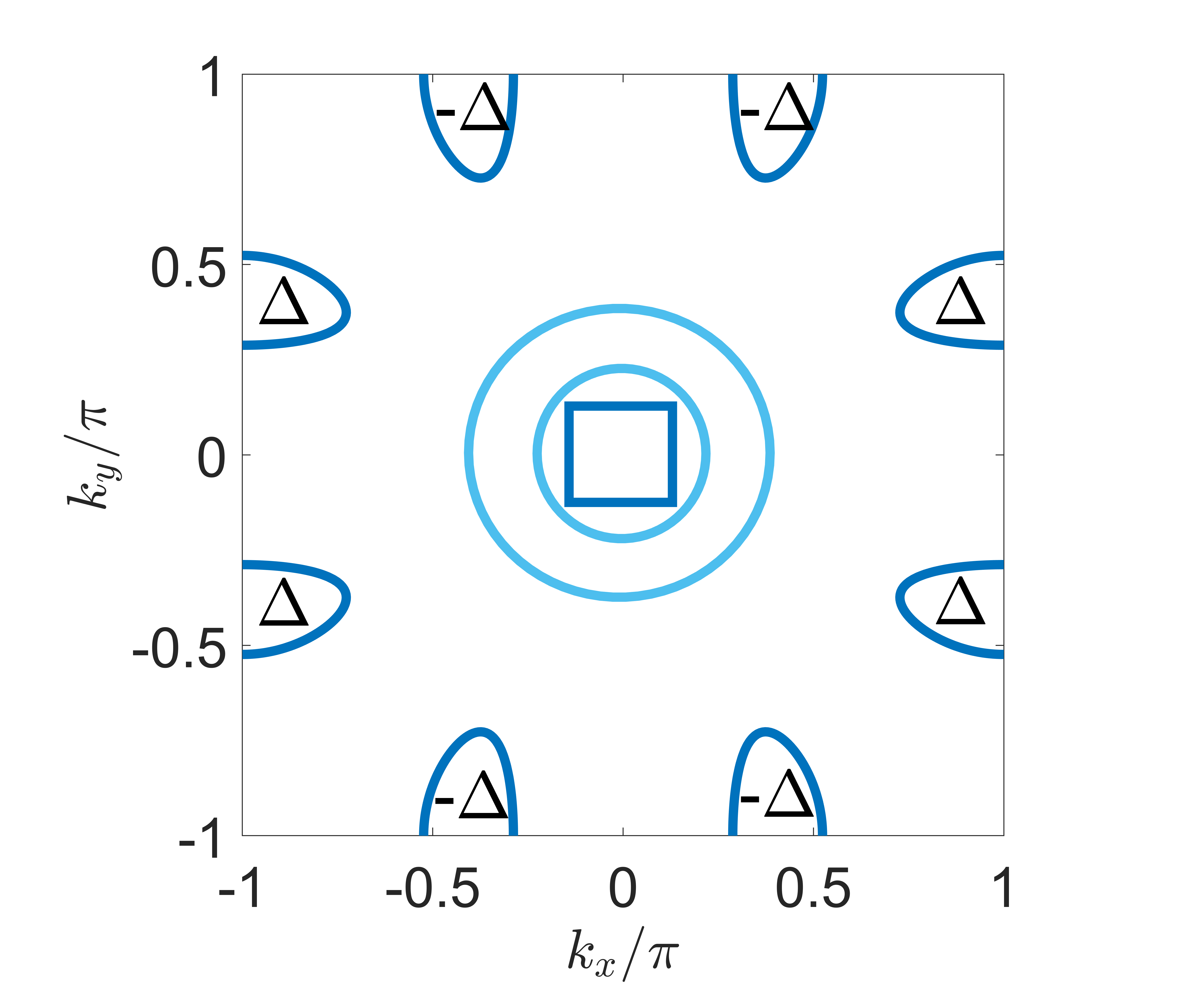
To describe theses beans, we develop a power series expansion in powers of $\delta k_{x},\delta k_{y}$ centered about the minima of the band along the X–M line. Explicitly considering a bean centered at $(k_{x},k_{y})=\left(\frac{\pi}{a},\frac{0.4\pi}{a}\right)$, we have the dispersion

Mirror symmetry prevents terms odd in $\delta k_{x}$ appearing in this expression. We also expand $\xi_{-,\boldsymbol{k}}$ in Eq.  2 around the centers of the beans. For the pocket centered at $\left(\frac{\pi}{a},\frac{0.4\pi}{a}\right),\xi_{-,\boldsymbol{k}}=$ $\tilde{\lambda}\delta k_{x}a\sin k_{z}$.

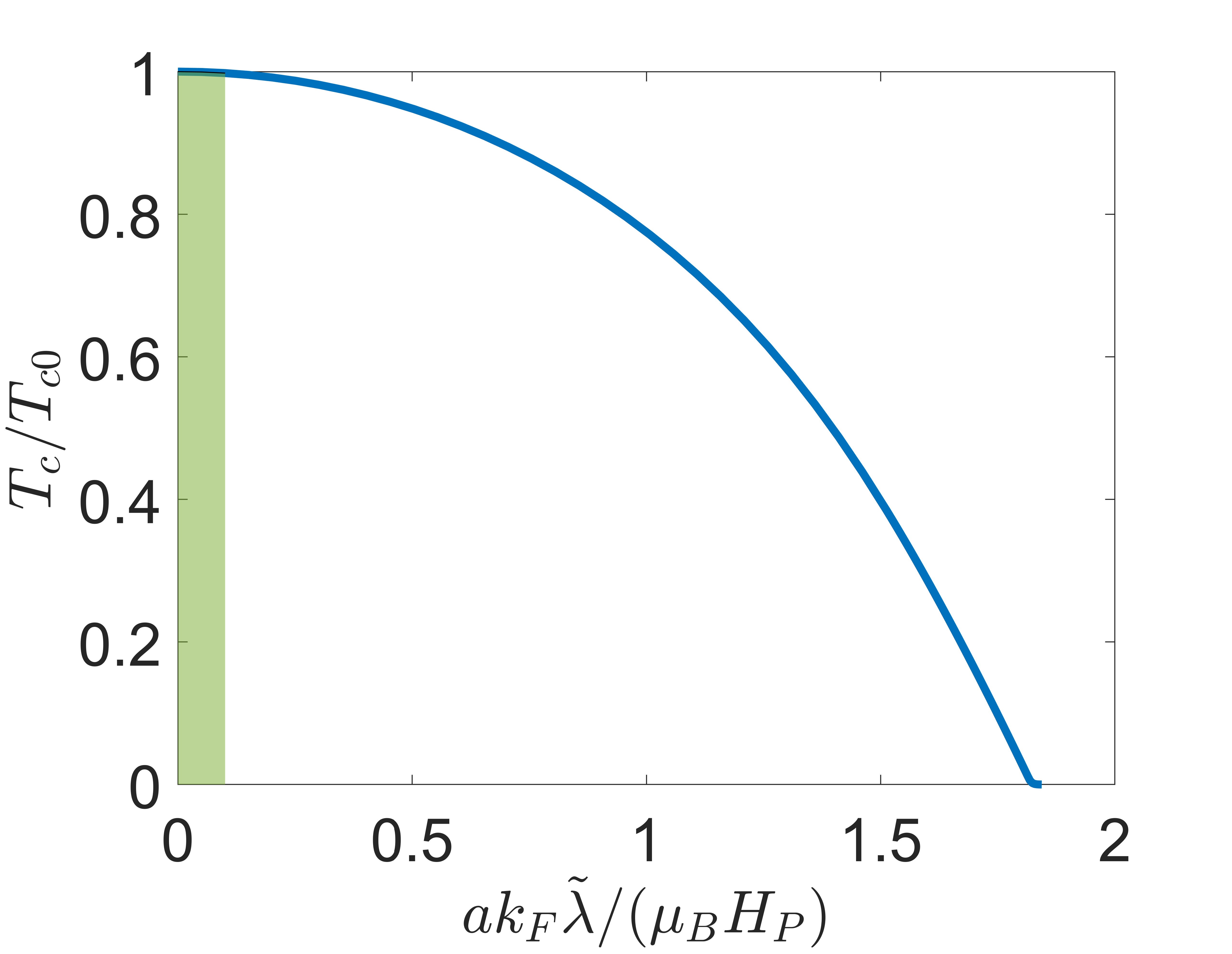
The numerical solution of the linearized gap equation is shown in Fig. 2. Because the Kramers’ degenerate magnetic order does not belong to a vector representation, a PDW state is not required by symmetry in this case. Thus when $\xi_{-,\boldsymbol{k}}$ becomes sufficiently large, superconductivity is suppressed as seen in Fig. 2. However, this is not observed in experiment Kibune et al. 2022; Kitagawa et al. 2022, which raises the question, how does superconductivity still survive. Here we suggest that the explanation for this persistence hinges on the value of $\tilde{\lambda}$ defined above. $\tilde{\lambda}$ on the beans is determined by the ratio of the Ising coupling ($\lambda$) to the Rashba spin-orbit coupling ($\alpha_{R}$) which occur in Eq. 1. In particular, using effective $g$ factors from DFT based renormalized band structure calculations we constrain $\tilde{\lambda}<0.2M_{z}$ Shishidou 2023. The critical temperature of $M_{z}$ is of the order of the critical temperature of superconductivity, hence $M_{z}\approx\mu_{B}H_{P}$ thus $\tilde{\lambda}<0.2\mu_{B}H_{P}$. We further estimate $a\text{k}_{F}\approx\frac{1}{2}$. Hence $\frac{a\text{k}_{F}\tilde{\lambda}}{\mu_{B}H_{P}}<0.1$. This is shown as the shaded region in Fig.  2. Thus superconductivity still persists despite the presence of Kramers’ degenerate magnetic order.

While the pairing state we consider above has $d_{x^{2}-y^{2}}$ symmetry, it is nodeless on the Fermi surface beans which do not intersect the $d_{x^{2}-y^{2}}$ nodes. However, the $d_{x^{2}-y^{2}}$ gap will have nodes along on the $\Gamma$-centered Fermi surfaces, possibly allowing for Bogoliubov Fermi surfaces to appear in the superconducting state. However, these nodes will not be inflated to Bogoliubov Fermi surfaces since $(\Delta\varepsilon)_{\boldsymbol{k}}$ vanishes along the diagonal the nodes. We can further consider other gap functions with nodes to see if Bogoliubov Fermi surfaces are expected. For example, nodes can appear on the beans for a $d_{xy}$ like gap. The beans will then have nodes where they intersect the Brillouin Zone face. However, these nodes will also not be inflated to form Bogoliubov Fermi surfaces because again $(\Delta\varepsilon)_{\boldsymbol{k}}$ vanishes on this face. Consequently, we do not expect Bogoliubov Fermi surfaces to appear as a consequence of the Kramer’s degenerate magnetic order in CeRh₂As₂ for any pairing symmetry.

Remarkably, the maximum $J$ value for the PDW state is about 15 times larger than the $\boldsymbol{q}=0$ state. In addition, since the $d$-wave gap has nodes, the loop current order will give rise to BFSs. This has been examined previously when there is no PDW order Berg et al. 2008; Kivelson and Varma 2012; Wang and Vafek 2013. As shown in Fig. 4, we find that the BFS are strongly shrunk due to the PDW order. The gain in condensation energy due to the shrinking of the BFS provides an energetic mechanism to stabilize the PDW state.

References

- Khim et al. (2021) S. Khim, J. Landaeta, J. Banda, N. Bannor, M. Brando, P. M. R. Brydon, D. Hafner, R. Küchler, R. Cardoso-Gil, U. Stockert, A. P. Mackenzie, D. F. Agterberg, C. Geibel, and E. Hassinger, Field-induced transition within the superconducting state of , Science 373, 1012 (2021).
- Schertenleib et al. (2021) E. G. Schertenleib, M. H. Fischer, and M. Sigrist, Unusual phase diagram of : The role of staggered noncentrosymmetricity, Phys. Rev. Research 3, 023179 (2021).
- Ptok et al. (2021) A. Ptok, K. J. Kapcia, P. T. Jochym, J. Łażewski, A. M. Oleś, and P. Piekarz, Electronic and dynamical properties of : Role of layers and expected orbital order, Phys. Rev. B 104, L041109 (2021).
- Möckli and Ramires (2021) D. Möckli and A. Ramires, Two scenarios for superconductivity in , Phys. Rev. Research 3, 023204 (2021).
- Skurativska et al. (2021) A. Skurativska, M. Sigrist, and M. H. Fischer, Spin response and topology of a staggered-Rashba superconductor, Phys. Rev. Research 3, 033133 (2021).
- Nogaki et al. (2021) K. Nogaki, A. Daido, J. Ishizuka, and Y. Yanase, Topological crystalline superconductivity in locally noncentrosymmetric , Physical Review Research 3, L032071 (2021).
- Cavanagh et al. (2022) D. Cavanagh, T. Shishidou, M. Weinert, P. M. R. Brydon, and D. F. Agterberg, Nonsymmorphic symmetry and field-driven odd-parity pairing in , Physical Review B 105, L020505 (2022).
- Landaeta et al. (2022) J. Landaeta, P. Khanenko, D. Cavanagh, C. Geibel, S. Khim, S. Mishra, I. Sheikin, P. M. R. Brydon, D. F. Agterberg, M. Brando, et al., Field-angle dependence reveals odd-parity superconductivity in , Physical Review X 12, 031001 (2022).
- Nogaki and Yanase (2022) K. Nogaki and Y. Yanase, Even-odd parity transition in strongly correlated locally noncentrosymmetric superconductors: Application to , Physical Review B 106, L100504 (2022).
- Möckli and Ramires (2021) D. Möckli and A. Ramires, Superconductivity in disordered locally noncentrosymmetric materials: An application to , Physical Review B 104, 134517 (2021).
- Hazra and Coleman (2022) T. Hazra and P. Coleman, Triplet pairing mechanisms from Hund’s-Kondo models: applications to and , arXiv preprint arXiv:2205.13529 (2022).
- Mishra et al. (2022) S. Mishra, Y. Liu, E. D. Bauer, F. Ronning, and S. M. Thomas, Anisotropic magnetotransport properties of the heavy-fermion superconductor , Physical Review B 106, L140502 (2022).
- Kimura et al. (2021) S.-i. Kimura, J. Sichelschmidt, and S. Khim, Optical study of the electronic structure of locally noncentrosymmetric , Physical Review B 104, 245116 (2021).
- Machida (2022) K. Machida, Violation of Pauli-Clogston limit in the heavy-fermion superconductor : Duality of itinerant and localized 4 f electrons, Physical Review B 106, 184509 (2022).
- Semeniuk et al. (2023) K. Semeniuk, D. Hafner, P. Khanenko, T. Lühmann, J. Banda, J. F. Landaeta, C. Geibel, S. Khim, E. Hassinger, and M. Brando, Superconductivity versus quadrupole density wave in , arXiv preprint arXiv:2301.09151 (2023).
- Onishi et al. (2022) S. Onishi, U. Stockert, S. Khim, J. Banda, M. Brando, and E. Hassinger, Low-temperature thermal conductivity of the two-phase superconductor , Frontiers in Electronic Materials 2 (2022).
- Kibune et al. (2022) M. Kibune, S. Kitagawa, K. Kinjo, S. Ogata, M. Manago, T. Taniguchi, K. Ishida, M. Brando, E. Hassinger, H. Rosner, et al., Observation of antiferromagnetic order as odd-parity multipoles inside the superconducting phase in , Physical Review Letters 128, 057002 (2022).
- Kitagawa et al. (2022) S. Kitagawa, M. Kibune, K. Kinjo, M. Manago, T. Taniguchi, K. Ishida, M. Brando, E. Hassinger, C. Geibel, and S. Khim, Two-dimensional xy-type magnetic properties of locally noncentrosymmetric superconductor , Journal of the Physical Society of Japan 91, 043702 (2022).
- Sumita and Yanase (2016) S. Sumita and Y. Yanase, Superconductivity in magnetic multipole states, Physical Review B 93, 224507 (2016).
- Hayami et al. (2018) S. Hayami, M. Yatsushiro, Y. Yanagi, and H. Kusunose, Classification of atomic-scale multipoles under crystallographic point groups and application to linear response tensors, Physical Review B 98, 165110 (2018).
- (21) H. Wu, A. Amin, Y. Yu, and D. F. Agterberg, submitted to Physical Review Letters (2023).
- Sumita et al. (2017) S. Sumita, T. Nomoto, and Y. Yanase, Multipole superconductivity in nonsymmorphic Sr2IrO4, Physical Review Letters 119, 027001 (2017).
- Berg et al. (2008) E. Berg, C.-C. Chen, and S. A. Kivelson, Stability of nodal quasiparticles in superconductors with coexisting orders, Physical Review Letters 100, 027003 (2008).
- Allais and Senthil (2012) A. Allais and T. Senthil, Loop current order and d-wave superconductivity: Some observable consequences, Physical Review B 86, 045118 (2012).
- Wang and Vafek (2013) L. Wang and O. Vafek, Quantum oscillations of the specific heat in d-wave superconductors with loop current order, Physical Review B 88, 024506 (2013).
- Nagashima et al. (2022) T. Nagashima, T. Hashimoto, S. Najafzadeh, S.-i. Ouchi, T. Suzuki, A. Fukushima, S. Kasahara, K. Matsuura, M. Qiu, Y. Mizukami, K. Hashimoto, Y. Matsuda, T. Shibauchi, S. Shin, and K. Okazaki, Discovery of nematic Bogoliubov Fermi surface in an iron-chalcogenide superconductor, Research Square preprint https://doi.org/10.21203/rs.3.rs-2224728/v1 (2022).
- Fedchenko et al. (2022) O. Fedchenko, L. Šmejkal, M. Kallmayer, Y. Lytvynenko, K. Medjanik, S. Babenkov, D. Vasilyev, M. Klaeui, J. Demsar, G. Schönhense, et al., Direct observation of antiferromagnetic parity violation in the electronic structure of Mn2Au, Journal of Physics: Condensed Matter 34, 425501 (2022).
- Šmejkal et al. (2017) L. Šmejkal, J. Železnỳ, J. Sinova, and T. Jungwirth, Electric control of dirac quasiparticles by spin-orbit torque in an antiferromagnet, Physical Review Letters 118, 106402 (2017).
- Urru et al. (2022) A. Urru, J.-R. Soh, N. Qureshi, A. Stunault, B. Roessli, H. M. Rønnow, and N. A. Spaldin, Neutron scattering from local magnetoelectric multipoles: a combined theoretical, computational, and experimental perspective, arXiv preprint arXiv:2212.06779 (2022).
- Bhowal and Spaldin (2021) S. Bhowal and N. A. Spaldin, Revealing hidden magnetoelectric multipoles using compton scattering, Physical Review Research 3, 033185 (2021).
- Spaldin and Ramesh (2019) N. Spaldin and R. Ramesh, Advances in magnetoelectric multiferroics, Nature Materials 18, 203 (2019).
- Yatsushiro et al. (2022) M. Yatsushiro, R. Oiwa, H. Kusunose, and S. Hayami, Analysis of model-parameter dependences on the second-order nonlinear conductivity in -symmetric collinear antiferromagnetic metals with magnetic toroidal moment on zigzag chains, Phys. Rev. B 105, 155157 (2022).
- Hayami et al. (2022) S. Hayami, M. Yatsushiro, and H. Kusunose, Nonlinear spin hall effect in -symmetric collinear magnets, Phys. Rev. B 106, 024405 (2022).
- Varma (1997) C. Varma, Non-Fermi-liquid states and pairing instability of a general model of copper oxide metals, Physical Review B 55, 14554 (1997).
- Varma (1999) C. Varma, Pseudogap phase and the quantum-critical point in copper-oxide metals, Physical Review Letters 83, 3538 (1999).
- Simon and Varma (2002) M. Simon and C. Varma, Detection and implications of a time-reversal breaking state in underdoped cuprates, Physical Review Letters 89, 247003 (2002).
- Varma (2006) C. Varma, Theory of the pseudogap state of the cuprates, Physical Review B 73, 155113 (2006).
- Sigrist and Ueda (1991) M. Sigrist and K. Ueda, Phenomenological theory of unconventional superconductivity, Reviews of Modern physics 63, 239 (1991).
- Gor’kov and Rashba (2001) L. P. Gor’kov and E. I. Rashba, Superconducting 2d system with lifted spin degeneracy: mixed singlet-triplet state, Physical Review Letters 87, 037004 (2001).
- Serene and Rainer (1983) J. Serene and D. Rainer, The quasiclassical approach to superfluid 3He , Physics Reports 101, 221 (1983).
- Agterberg et al. (2020) D. F. Agterberg, J. S. Davis, S. D. Edkins, E. Fradkin, D. J. V. Harlingen, S. A. Kivelson, P. A. Lee, L. Radzihovsky, J. M. Tranquada, and Y. Wang, The physics of pair-density waves: Cuprate superconductors and beyond, Annual Review of Condensed Matter Physics 11, 231 (2020).
- Yuan and Fu (2022) N. F. Yuan and L. Fu, Supercurrent diode effect and finite-momentum superconductors, Proceedings of the National Academy of Sciences 119, e2119548119 (2022).
- He et al. (2022) J. J. He, Y. Tanaka, and N. Nagaosa, A phenomenological theory of superconductor diodes, New Journal of Physics 24, 053014 (2022).
- Daido et al. (2022) A. Daido, Y. Ikeda, and Y. Yanase, Intrinsic superconducting diode effect, Physical Review Letters 128, 037001 (2022).
- Pal et al. (2022) B. Pal, A. Chakraborty, P. K. Sivakumar, M. Davydova, A. K. Gopi, A. K. Pandeya, J. A. Krieger, Y. Zhang, M. Date, S. Ju, et al., Josephson diode effect from cooper pair momentum in a topological semimetal, Nature Physics 18, 1228 (2022).
- Agterberg et al. (2017) D. F. Agterberg, P. M. R. Brydon, and C. Timm, Bogoliubov Fermi surfaces in superconductors with broken time-reversal symmetry, Physical review letters 118, 127001 (2017).
- Brydon et al. (2018) P. M. R. Brydon, D. F. Agterberg, H. Menke, and C. Timm, Bogoliubov Fermi surfaces: General theory, magnetic order, and topology, Physical Review B 98, 224509 (2018).
- Link and Herbut (2020) J. M. Link and I. F. Herbut, Bogoliubov-Fermi surfaces in noncentrosymmetric multicomponent superconductors, Physical Review Letters 125, 237004 (2020).
- Timm et al. (2017) C. Timm, A. Schnyder, D. F. Agterberg, and P. M. R. Brydon, Inflated nodes and surface states in superconducting half-heusler compounds, Physical Review B 96, 094526 (2017).
- Hafner et al. (2022) D. Hafner, P. Khanenko, E.-O. Eljaouhari, R. Küchler, J. Banda, N. Bannor, T. Lühmann, J. Landaeta, S. Mishra, I. Sheikin, et al., Possible quadrupole density wave in the superconducting kondo lattice , Physical Review X 12, 011023 (2022).
- Shishidou (2023) T. Shishidou (2023), in preparation.
- Kivelson and Varma (2012) S. Kivelson and C. Varma, Fermi pockets in a d-wave superconductor with coexisting loop-current order, arXiv preprint arXiv:1208.6498 (2012).
Appendices
Appendix A Appendix A: Derivation of the Green’s functions
Starting from the single-band Hamiltonian