Beyond Normal: On the Evaluation of Mutual Information Estimators
Abstract
Mutual information is a general statistical dependency measure which has found applications in representation learning, causality, domain generalization and computational biology. However, mutual information estimators are typically evaluated on simple families of probability distributions, namely multivariate normal distribution and selected distributions with one-dimensional random variables. In this paper, we show how to construct a diverse family of distributions with known ground-truth mutual information and propose a language-independent benchmarking platform for mutual information estimators. We discuss the general applicability and limitations of classical and neural estimators in settings involving high dimensions, sparse interactions, long-tailed distributions, and high mutual information. Finally, we provide guidelines for practitioners on how to select appropriate estimator adapted to the difficulty of problem considered and issues one needs to consider when applying an estimator to a new data set.
1 Introduction
Estimating the strength of a non-linear dependence between two continuous random variables (r.v.) lies at the core of machine learning. Mutual information (MI) lends itself naturally to this task, due to its desirable properties, such as invariance to homeomorphisms and the data processing inequality. It finds applications in domain generalization (Li et al. 2022; Ragonesi et al. 2021), representation learning (Belghazi et al. 2018; Oord et al. 2018), causality (Solo 2008; Kurutach et al. 2018), physics (Keys et al. 2015), systems biology (Selimkhanov et al. 2014; Grabowski et al. 2019; Uda 2020), and epidemiology (Young et al. 2023).
Over the last decades, the estimation of MI has been extensively studied, and estimators have been developed, ranging from classical approaches based on histogram density (Pizer et al. 1987), kernel density estimation (Moon et al. 1995) to -nearest neighbor (Kozachenko and Leonenko 1987; Kraskov et al. 2004) and neural estimators (Belghazi et al. 2018; Oord et al. 2018; Song and Ermon 2020). However, despite the progress that has been achieved in this area, not much attention has been focused on systematically benchmarking these approaches.
Typically, new estimators are evaluated assuming multivariate normal distributions for which MI is analytically tractable (Darbellay and Vajda 1999; Kraskov et al. 2004; Suzuki 2016). Sometimes, simple transformations are applied to the data (Khan et al. 2007; Gao et al. 2015), moderately high-dimensional settings are considered (Lord et al. 2018; Lu and Peltonen 2020), or strong dependencies are evaluated (Gao et al. 2015). Beyond that, Song and Ermon 2020 study the self-consistency (additivity under independence and the data processing inequality) of neural MI estimators in the context of representation learning from image data.
Our Contributions In this work we show a method of developing expressive distributions with known ground-truth mutual information (Sec. 2), propose forty benchmark tasks and systematically study the properties of commonly used estimators, including representatives based on kernel or histogram density estimation, NN estimation, and neural network-based estimators (Sec. 3). We address selected difficulties one can encounter when estimating mutual information (Sec. 4), such as sparsity of interactions, long-tailed distributions, invariance, and high mutual information. Finally, we provide recommendations for practitioners on how to choose a suitable estimator for particular problems (Sec. 6). Our benchmark is designed so that it is simple to add new tasks and estimators. It also allows for cross-language comparisons — in our work we compare estimators implemented in Python, R and Julia. All of our experiments are fully reproducible by running Snakemake workflows (Mölder et al. 2021). Accompanying code is available at http://github.com/cbg-ethz/bmi.

Overall, our key findings from the benchmark can be summarized as follows:
- •
Testing on multivariate normal distributions gives a biased and overly optimistic view of estimator performance. In this setting, canonical correlation analysis (CCA), a model-based approach, emerges as the most effective method — even if the model is slightly misspecified.
- •
Compared to classical estimators, neural estimators excel in high-dimensional settings, capturing sparse interactions across multiple dimensions.
- •
The popular KSG estimator (Kraskov et al. 2004) is accurate in low- and moderate-dimensional settings, but its performance suffers on problems involving high-dimensions or sparse interactions.
- •
Although MI is invariant to a wide range of transformations (Theorem 2.1), numerical estimates, even with large sample sizes, are not. Thus, MI may not be suitable when metric invariance to specific transformation families is required.
- •
Multivariate Student distributions pose an important and hard challenge to many mutual information estimators. This effect is partially, but not fully, attributed to their long tails.
2 Mutual Information: Estimation and Invariance
We start by recalling the definition of MI, then discuss the problem of estimating it, and introduce the estimators used in the benchmark.
Consider two r.v. and with domains respectively , joint probability measure and marginal probability measures and , respectively. If is absolutely continuous with respect to (e.g., and are finite r.v.), MI is equal to the following Kullback--Leibler divergence11 1 We use the natural logarithm, meaning that the mutual information is measured in nats.:
where is the Radon–Nikodym derivative. If the absolute continuity does not hold, then (Pinsker and Feinstein 1964, Theorem 2.1.2). If and are Euclidean spaces and measures , and have probability density functions (PDFs) with respect to the Lebesgue measure, then the Kullback–Leibler divergence can be written in terms of the PDFs. However, we will later consider distributions which do not have PDFs with respect to the Lebesgue measure and the general Radon–Nikodym derivative must be used (see “Swiss roll” in Fig. 1).
In almost all applications, and are not known and one needs to estimate MI from a finite sample from , i.e., a realization of i.i.d. r.v. distributed according to the joint distribution . As a MI estimator we will denote a family of measurable mappings, indexed by the sample size and spaces and (in most applications, Euclidean spaces of various dimensionalities): Composing this mapping with the r.v. representing the whole data set we obtain a real-valued r.v. For a given we can consider the distribution of . It is often summarized by its first two moments, resulting in the bias and the variance of the estimator. Understanding the bias of an estimator however requires the knowledge of ground-truth MI, so the estimators are typically tested on the families of jointly multivariate normal or uniform distributions, with varying and ground-truth (Khan et al. 2007; Lord et al. 2018; Holmes and Nemenman 2019; Song and Ermon 2020).
Constructing Expressive Distributions and Benchmarking Besides considering different types of distributions such as (multivariate) normal, uniform and Student, our benchmark is based on the invariance of MI to the family of chosen mappings. Generally MI is not invariant to arbitrary transformations, as due to the data processing inequality . However, under some circumstances MI is preserved, which enables us to create more expressive distributions by transforming the variables.
Theorem 2.1.
Let , , and be standard Borel spaces (e.g., smooth manifolds with their Borel -algebras) and and be continuous injective mappings. Then, for every -valued r.v. and -valued r.v. it holds that
This theorem has been studied before by Kraskov et al. 2004, who consider diffeomorphisms and by Polyanskiy and Wu 2022, who assume measurable injective functions with measurable left inverses. For completeness we provide a proof which covers continuous injective mappings in Appendix A. In particular, each of and can be a homeomorphism, a diffeomorphism, or a topological embedding. Embeddings are allowed to increase the dimensionality of the space, so even if and have probability density functions, and do not need to have them. Neither of these deformations change MI. Thus, using Theorem 2.1, we can create more expressive distributions by sampling from and transforming the samples to obtain a data set
While offering a tool to construct expressive distributions, another valuable perspective to consider with this problem is estimation invariance: although MI is invariant to proposed changes, the estimate may not be. More precisely, applying an estimator to the transformed data set results in the induced r.v. and its distribution. If the estimator were truly invariant, one would expect that should equal . This invariance is rarely questioned and often implicitly assumed as given (see e.g. Tschannen et al. 2020 or Murphy 2023), but as we will see in Sec. 4.3, finite-sample estimates are not generally invariant.
3 Proposed Benchmark
In this section, we outline forty tasks included in the benchmark that cover a wide family of distributions, including varying tail behaviour, sparsity of interactions, multiple modes in PDF, and transformations that break colinearity. As our base distributions, we selected multivariate normal and Student distributions, which were transformed with continuous injective mappings.
We decided to focus on the following phenomena:
- 1.
Dimensionality. High-dimensional data are collected in machine learning and natural sciences (Bühlmann and van de Geer 2011, Ch. 1). We therefore change the dimensions of the and spaces between and .
- 2.
Sparsity. While the data might be high-dimensional, the effective dimension may be much smaller, due to correlations between different dimensions or sparsity (Lucas et al. 2006). We therefore include distributions in which some of the dimensions represent random noise, which does not contribute to the mutual information, and perform an additional study in Section 4.1.
- 3.
Varying MI. Estimating high MI is known to be difficult (McAllester and Stratos 2020). However, we can often bound it in advance — if there are 4000 image classes, MI between image class and representation is at most nats. In this section, we focus on problems with MI varying up to 2 nats. We additionally consider distributions with higher MI in Section 4.4.
- 4.
Long tails. As Taleb 2020 and Zhang et al. 2021 argue, many real-world distributions have long tails. To model different tails we consider multivariate Student distributions as well as transformations lengthening the tails. We conduct an additional study in Section 4.2.
- 5.
Robustness to diffeomorphisms. As stated in Theorem 2.1, mutual information is invariant to reparametrizations of random variables by diffeomorphisms. We however argue that when only finite samples are available, invariance in mutual information estimates may not be achieved. To test this hypothesis we include distributions obtained by using a diverse set of diffeomorphisms and continuous injective mappings. We further study the robustness to reparametrizations in Section 4.3.
While we provide a concise description here, precise experimental details can be found in Appendix D and we visualise selected distributions in Appendix F. We first describe tasks employing one-dimensional variables.
Bivariate Normal For multivariate normal variables MI depends only on the correlation matrix. We will therefore consider a centered bivariate normal distribution with and . We chose .
Uniform Margins As a first transformation, we apply the Gaussian CDF to Gaussian r.v. and to obtain r.v. and . It is a standard result in copula theory (see Lemma D.2 or e.g., Nelsen 2007 for an introduction to copulas) that resp. . The joint distribution , however, is not uniform. Mutual information is preserved, . For an illustration, see Fig. 1. A distribution P transformed with Gaussian CDF will be denoted as Normal CDF @ P.
Half-Cube Map To lengthen the tails we applied the half-cube homeomorphism to Gaussian variables and . We visualize an example in Fig. 1 and denote a transformed distribution as Half-cube @ P.
Asinh Mapping To shorten the tails we applied inverse hyperbolic sine function . A distribution transformed with this mapping will be denoted as Asinh @ P.
Wiggly Mapping To model non-uniform lengthscales, we applied a mapping
Due to the inequality constraint this mapping is injective and preserves MI. The parameter values can be found in Appendix D. We denote the transformed distribution as Wiggly @ P.
Bimodal Variables Applying the inverse CDF of a two-component Gaussian mixture model to correlated variables and with uniform margins we obtained a joint probability distribution with four modes (presented in Fig. 1). We call this distribution Bimodal and provide technical details in Appendix D.
Additive Noise Consider independent r.v. and , where is the noise level. For , it is possible to derive analytically (see Appendix D for the formula and the parameter values) and we will call this distribution Uniform (additive noise=).
Swiss Roll Embedding As the last example in this section, we consider a mixed case in which a one-dimensional r.v. is smoothly embedded into two dimensions via the Swiss roll mapping, a popular embedding used to test dimensionality reduction algorithms (see Fig. 1 for visualisation and Appendix D for the formula). Note that the obtained distribution does not have a PDF with respect to the Lebesgue measure on .
Next, we describe the tasks based on multivariate distributions.
Multivariate Normal We sampled from the multivariate normal distribution. We model two correlation structures: “dense” interactions with all off-diagonal correlations set to 0.5 and “2-pair” interactions where and there is no correlation between any other (distinct) variables (Multinormal (2-pair)). For a latent-variable interpretation of these covariance matrices we refer to Appendix D.2.
Multivariate Student To see how well the estimators can capture MI contained in the tails of the distribution, we decided to use multivariate Student distributions (see Appendix D) with dispersion matrix22 2 The dispersion matrix of multivariate Student distribution is different from its covariance, which does not exist for . set to the identity and degrees of freedom. Contrary to the multivariate normal case, in which the identity matrix used as the covariance would lead to zero MI, the variables and can still interact through the tails.
Transformed Multivariate Distributions As the last set of benchmark tasks we decided to transform the multivariate normal and multivariate Student distributions. We apply mappings described above to each axis separately. For example, applying normal CDF to the multivariate normal distribution will map it into a distribution over the cube with uniform marginals. To mix different axes we used a spiral diffeomorphism (denoted as Spiral @ P); we defer the exact construction to Appendix D but we visualise this transformation in Fig. 5.
Estimators In our benchmark, we include a diverse set of estimators. Following recent interest, we include four neural estimators, i.e., Donsker–Varadhan (D-V) and MINE (Belghazi et al. 2018), InfoNCE (Oord et al. 2018), and the NWJ estimator (Nguyen et al. 2007; Nowozin et al. 2016; Poole et al. 2019). As a representative for model-based estimators, we implement an estimator based on canonical correlation analysis (CCA) (Murphy 2023, Ch. 28), which assumes that the joint distribution is multivariate normal. For more classical estimators, we include the Kraskov, Stögbauer and Grassberger (KSG) estimator (Kraskov et al. 2004) as the most well-known -nearest neighbour-based estimator, a recently proposed kernel-based estimator (LNN) (Gao et al. 2017b), as well as an estimator based on histograms and transfer entropy (both implemented in Julia’s TransferEntropy library). A detailed overview of the different classes of estimators is provided in Appendix C. Further, we describe the the hyperparameter selection in Appendix E.
Preprocessing As a data preprocessing step, we standardize each dimension using the mean and standard deviation calculated from the sample. Other preprocessing stategies are also possible, but we did not observe a consistent improvement of one preprocessing strategy over the others (see Appendix E).
3.1 Benchmark Results
We show the results for data points in Fig. 2. Neural estimators and KSG perform better than alternative estimators on most problems, with KSG having often low sample requirements (see Appendix E). The simple model-based estimator CCA obtained excellent performance at low sample sizes (see Appendix E), even for slightly transformed multivariate normal distributions. Finally, LNN and the two Julia estimators (histogram and transfer entropy), work well in low dimension but are not viable in medium- and high-dimensional problems ().
Overall, we observed that for most -dimensional and multivariate normal problems MI can be reliably estimated. Difficulties arise for sparse interactions, atypical (Student) distributions, and for significantly transformed distributions. This suggests that the typical evaluations of MI estimators are overly optimistic, focusing on relatively simple problems.
KSG is able to accurately estimate MI in multivariate normal problems, however performance drops severely on tasks with sparse interactions (2-pair tasks). For dimensions the estimate is about 70% of the true MI, and for dimensions it drops to 10%, which is consistent with previous observations (Marx and Fischer 2022). Meanwhile, performance of neural estimators is stable. We study the effect of sparsity in more detail in Sec. 4.
Student distributions have proven challenging to all estimators. This is partially due to the fact that long tails can limit estimation quality (see Sec. 4), and indeed, applying a tail-shortening transformation improves performance. However, performance still remains far below multivariate normal distributions with similar dimensionality and information content, showing that long tails are only part of the difficulty. For neural estimators, the issue could be explained by the fact that the critic is not able to fully learn the pointwise mutual information (see Appendix E).
Interestingly, the performance of CCA, which assumes a linear Gaussian model, is often favorable compared to other approaches and has very low sample complexity (see Appendix E). This is surprising, since in the case of transformed distributions the model assumptions are not met. The approach fails for Student distributions (for which the correlation matrix either does not exist or is the identity matrix), the Swiss roll embedding and multivariate normal distributions transformed using the spiral diffeomorphism. Since the spiral diffeomorphism proved to be the most challenging transformation, we study it more carefully in Sec. 4.
4 Selected Challenges
In this section we investigate distributions which proved to be particularly challenging for the tested estimators in our benchmark: sparse interactions, long tailed distributions and invariance to diffeomorphisms. Additionally we investigate how the estimators perform for high ground truth MI.
4.1 Sparsity of Interactions
In the main benchmark (Fig. 2) we observed that estimation of MI with “2-pair” type of interactions is considerably harder for the KSG estimator than the “dense” interactions. On the other hand, neural estimators were able to pick the relevant interacting dimensions and provide better estimates of MI in these sparse cases.
We decided to interpolate between the “dense” and “2-pair” interaction structures using a two-stage procedure with real parameters and and the number of strongly interacting components . While the precise description is in Appendix D.2, we can interpret as controlling the baseline strength of interaction between every pair of variables in and as the additional strength of interaction between pairs of variables . Dense interaction structure has and 2-pair interaction structure has and . First, we set and and decrease raising at the same time to maintain constant MI of 1 nat. When , whole information is contained in the pairwise interactions . We then decrease and increase , still maintaining constant MI.
In Fig. 3 we observe that the performance of all estimators considered (apart from CCA, a model-based approach suitable for multivariate normal distributions) degrades when the interactions between every pair of variables become sparser (lower ). In particular, even neural estimators are not able to model the information in ten interacting pairs of variables. However, when we decrease the number of interacting pairs of variables, the performance of the neighborhood-based KSG estimator is qualitatively different from the neural estimators: performance of KSG steadily deteriorates, while neural estimators can find (some of the) relevant pairs of variables.
This motivates us to conclude that in the settings where considered variables are high-dimensional and the interaction structure is sparse, neural estimators can offer an advantage over neighborhood-based approaches.
4.2 Long-Tailed Distributions
In Fig. 4 we investigate two different ways to lengthen the tails. First, we lengthen the tails of a multivariate normal distribution using the mapping (with ) applied to each dimension separately. In this case, we see that the performance of CCA, KSG, and neural estimators is near-perfect for close to (when the distribution is close to multivariate normal), but the performance degrades as the exponent increases. Second, we study multivariate Student distributions varying the degrees of freedom: the larger the degrees of freedom, the lower the information content in the tails of the distribution. Again, we see that that the performance of CCA, KSG, and neural estimators is near-perfect for high degrees of freedom for which the distribution is approximately normal. For low degrees of freedom, these estimators significantly underestimate MI, with the exception of CCA which gives estimates with high variance, likely due to the correlation matrix being hard to estimate.
Overall, we see that long tails complicate the process of estimating MI. The Student distribution is particularly interesting, since even after the tails are removed (with or preprocessing strategies described in Appendix E) the task remains challenging. We suspect that the MI might be contained in regions which are rarely sampled, making the MI hard to estimate. When neural estimators are used, pointwise mutual information learned by the critic does not match the ground truth (see Appendix E).
Hence, we believe that accurate estimation of MI in long-tailed distributions is an open problem. Practitioners expecting long-tailed distributions should approach this task with caution.
4.3 Invariance to Diffeomorphisms

The benchmark results (Fig. 2) as well as the experiments with function lengthening tails (Fig. 4) suggest that even if ground-truth MI is preserved by a transformation (see Theorem 2.1), the finite-sample estimates may not be invariant. This can be demonstrated using the spiral diffeomorphism.
We consider isotropic multivariate normal variables and with . Then, we apply a spiral diffeomorphism to , where
is the rotation around the origin by the angle (see Fig. 5; for a theoretical study of spiral diffeomorphisms see Appendix B). In Fig. 5, we present the estimates for , and varying speed .
In general, the performance of the considered estimators deteriorates with stronger deformations. This is especially visible for the CCA estimator, as MI cannot be reliably estimated in terms of correlation.
4.4 High Mutual Information
Gao et al. 2015 proves that estimation of MI between strongly interacting variables requires large sample sizes. Poole et al. 2019; Song and Ermon 2020 investigate estimation of high MI using multivariate normal distributions in the setting when the ground-truth MI is changing over the training time. We decided to use our family of expressive distributions to see the practical limitations of estimating MI. We chose three one-parameter distribution families: the multivariate normal distribution with correlation , and its transformations by the half-cube mapping and the spiral diffeomorphism with . We changed the parameter to match the desired MI.
In Fig. 6 we see that for low enough MI neural estimators and KSG reliably estimate MI for all considered distributions, but the moment at which the estimation becomes inaccurate depends on the distribution. For example, for Gaussian distributions, neural estimators (and the simple CCA baseline) are accurate even up to 5 nats, while after the application of the spiral diffeomorphism, the estimates become inaccurate already at 2 nats.
We see that in general neural estimators perform well on distributions with high MI. The performance of CCA on the multivariate normal distribution suggests that well-specified model-based estimators may require lower number of samples to estimate high mutual information than model-free alternatives (cf. Gao et al. 2015).
5 Related Work
| Khan et al. 2007 | Poole et al. 2019 | Song and Ermon 2020 | Proposed Benchmark | |
|---|---|---|---|---|
| Gaussian Distrib. | ✓ | ✓ | ✓ | ✓ |
| Heavy-Tailed Distrib. | (✓) | (✓) | ✓ | |
| Sparse/Dense Inter. | ✓ | |||
| High MI | (✓) | (✓) | ✓ | |
| Invariance to Homeom. | ✓ | |||
| Self-Consistency | ✓ | |||
| Language Indep. | ✓ | |||
| Code Available | ✓ | ✓ |
Existing Benchmarks Khan et al. 2007 used one-dimensional variables and an additive noise assumption to evaluate the estimators based on histograms, nearest neighbors, and kernels. However, the original code and samples are not available. Song and Ermon 2020 proposed to evaluate neural estimators based on variational lower bounds (Oord et al. 2018; Belghazi et al. 2018) on image data. However, besides the multivariate Gaussian which they also evaluate, the ground-truth MI is not available. Therefore, they proposed self-consistency checks, which include for independent and , and preservation of the data processing inequality. Poole et al. 2019 study neural estimators in settings employing Gaussian variables, affine transformation followed by axis-wise cubic transformation and investigate the high MI cases. In our benchmark, we focus on distributions with known MI and information-preserving continuous injective mappings such as homeomorphisms, evaluate heavy tail distributions, and compare representative estimators from different classes and platforms. We summarize the differences between the benchmarks in Table 1.33 3 Khan et al. 2007 consider two one-dimensional r.v. related by additive noise, in which one of the r.v. is parametrized with a cubic function. This implicitly lengthens the tails, so we marked this with (✓); similarly, Poole et al. 2019 consider cubic transformation of a multivariate normal variable. The experimental setup of estimation of MI considered by Poole et al. 2019 and Song and Ermon 2020 requires changing ground truth MI over training time of a neural estimator. This procedure differs from the usual approaches to estimating MI, so we marked it with (✓).
Causal Representation Learning and Nonlinear ICA Recent work on disentanglement and nonlinear independent component analysis (ICA) aims at identifying causal sources up to an ambiguous transformation (Xi and Bloem-Reddy 2022). Examples include orthogonal transformations (Zimmermann et al. 2021), permutations and diffeomorphisms applied along specific axes (Khemakhem et al. 2020), or the whole diffeomorphism group (Von Kügelgen et al. 2021; Daunhawer et al. 2023). To check whether the learned representations indeed capture underlying causal variables, it is important to use estimators which are invariant to the ambiguous transformations specific to the model. Our results suggest that such requirements are not met by MI estimators and practitioners should carefully choose the used metrics, so they are not only theoretically invariant, but also can be robustly estimated in practice.
6 Conclusions and Limitations
Venturing beyond the typical evaluation of mutual information estimators on multivariate normal distributions, we provided evidence that the evaluation on Gaussian distributions results in overly optimistic and biased results for existing estimators. In particular, a simple model-based approach as CCA is already sufficient if the distribution is (close to) multivariate normal, highlighting the effect of using available prior information about the problem to design efficient estimators. To provide a basis for more thorough evaluation, we designed a benchmark, compatible with any programming language, with forty general tasks focusing on selected problems, as estimation with sparse interactions, the effects of long tails, estimation in problems with high MI, and (only theoretical) invariance to diffeomorphisms.
Our results suggest that in low- and medium-dimensional problems the KSG estimator remains a solid baseline, requiring a lower number of samples than the alternatives and no parameter tuning. In high-dimensional settings where the interactions are sparse, neural estimators offer an advantage over classical estimators being able to more consistently pick up the signal hidden in the high-dimensional space. We further provide evidence that although MI is invariant to continuous injective transformations of variables, in practice the estimates can differ substantially. Appropriate data preprocessing may mitigate some of these issues, but no strategy clearly outperforms the others (see Appendix E).
We hope that the proposed benchmark encourages the development of new estimators, which address the challenges that we highlight in this paper. It can be used to assess invariance to homeomorphisms, understand an estimator’s behavior in the situations involving distributions of different complexity, low-data behaviour, high mutual information or to diagnose problems with implementations. We believe that some parts of the benchmark could also be used to assess whether other estimators of other statistical quantities, such as kernel dependence tests, transfer entropy or representation similarity measures, can be reliably estimated on synthetic problems and if they are robust to selected classes of transformations.
Limitations and Open Problems
Although the proposed benchmark covers a wide family of distributions, its main limitation is the possibility to only transform the distribution via transformations to starting from multivariate normal and Student distributions. In particular, not every possible joint distribution is of this form and extending the family of distributions which have known MI and allow efficient sampling is the natural direction of continuation. We are, however, confident that due to the code design it will be easy to extend the benchmark with the new distributions (and their transformations) when they appear.
Estimation of information in multivariate Student distributions remains a challenge for most estimators. Although we provide the evidence that distributions with longer tails pose a harder challenge for considered estimators, shortening the tails with transform did not alleviate all the issues. In neural estimators this can be partly explained by the fact that the critic may not learn to approximate pointwise mutual information (up to an additive constant) properly, as demonstrated in Appendix E, but the question of what makes the neighborhood-based estimator, KSG, fail, remains open.
As noted, unless strong inductive biases can be exploited (as illustrated for CCA), estimation of high MI is an important challenge. An interesting avenue towards developing new estimators can be by incorporating a stronger inductive bias, which could also take a form of development of better data normalization strategies and, in case of neural estimators, critic architectures. Better normalization strategies may make the estimators more invariant to considered transformations.
Acknowledgments and Disclosure of Funding
We would like to thank Craig Hamilton for the advice on scientific writing and help with the abstract. FG was supported by the Norwegian Financial Mechanism GRIEG-1 grant operated by Narodowe Centrum Nauki (National Science Centre, Poland) 2019/34/H/NZ6/00699. PC and AM were supported by a fellowship from the ETH AI Center.
References
- Ao and Li (2022) Ziqiao Ao and Jinglai Li. Entropy estimation via normalizing flow. Proceedings of the AAAI Conference on Artificial Intelligence, 36(9):9990–9998, 2022.
- Arellano-Valle et al. (2013) R.B. Arellano-Valle, J.E. Contreras-Reyes, and M.G. Genton. Shannon entropy and mutual information for multivariate skew-elliptical distributions. Scandinavian Journal of Statistics, 49:42–62, 2013.
- Belghazi et al. (2018) Mohamed Ishmael Belghazi, Aristide Baratin, Sai Rajeshwar, Sherjil Ozair, Yoshua Bengio, Aaron Courville, and Devon Hjelm. Mutual information neural estimation. In International conference on machine learning, pages 531–540. PMLR, 2018.
- Bradbury et al. (2018) James Bradbury, Roy Frostig, Peter Hawkins, Matthew James Johnson, Chris Leary, Dougal Maclaurin, George Necula, Adam Paszke, Jake VanderPlas, Skye Wanderman-Milne, and Qiao Zhang. JAX: composable transformations of Python+NumPy programs, 2018. URL http://github.com/google/jax.
- Bühlmann and van de Geer (2011) Peter Bühlmann and Sara van de Geer. Statistics for High-Dimensional Data: Methods, Theory and Applications. Springer Publishing Company, Incorporated, 1st edition, 2011. ISBN 3642201911.
- Cabeli et al. (2020) Vincent Cabeli, Louis Verny, Nadir Sella, Guido Uguzzoni, Marc Verny, and Hervé Isambert. Learning clinical networks from medical records based on information estimates in mixed-type data. PLOS Computational Biology, 16(5):e1007866, 2020.
- Carapetis (2022) Anthony Carapetis. Rotating spherical shells doesn’t change volume. Mathematics Stack Exchange, 2022. URL https://math.stackexchange.com/q/4500294. URL:https://math.stackexchange.com/q/4500294 (version: 2022-07-26).
- Cellucci et al. (2005) Christopher J Cellucci, Alfonso M Albano, and Paul E Rapp. Statistical validation of mutual information calculations: Comparison of alternative numerical algorithms. Physical review E, 71(6):066208, 2005.
- Cover and Thomas (2006) Thomas M. Cover and Joy A. Thomas. Elements of Information Theory. Wiley-Interscience New York, 2006.
- Darbellay and Vajda (1999) Georges A Darbellay and Igor Vajda. Estimation of the information by an adaptive partitioning of the observation space. IEEE Transactions on Information Theory, 45(4):1315–1321, 1999.
- Daub et al. (2004) Carsten O Daub, Ralf Steuer, Joachim Selbig, and Sebastian Kloska. Estimating mutual information using b-spline functions–an improved similarity measure for analysing gene expression data. BMC bioinformatics, 5(1):1–12, 2004.
- Daunhawer et al. (2023) Imant Daunhawer, Alice Bizeul, Emanuele Palumbo, Alexander Marx, and Julia E Vogt. Identifiability results for multimodal contrastive learning. In The Eleventh International Conference on Learning Representations, 2023. URL https://openreview.net/forum?id=U_2kuqoTcB.
- Gao et al. (2015) Shuyang Gao, Greg Ver Steeg, and Aram Galstyan. Efficient estimation of mutual information for strongly dependent variables. In Proceedings of the International Conference on Artificial Intelligence and Statistics (AISTATS), pages 277–286. PMLR, 2015.
- Gao et al. (2017a) Weihao Gao, Sreeram Kannan, Sewoong Oh, and Pramod Viswanath. Estimating mutual information for discrete-continuous mixtures. In Advances in Neural Information Processing Systems, pages 5986–5997, 2017a.
- Gao et al. (2017b) Weihao Gao, Sewoong Oh, and Pramod Viswanath. Density functional estimators with k-nearest neighbor bandwidths. In IEEE International Symposium on Information Theory (ISIT), pages 1351–1355. IEEE, 2017b.
- Gao et al. (2018) Weihao Gao, Sewoong Oh, and Pramod Viswanath. Demystifying fixed k-nearest neighbor information estimators. IEEE Transactions on Information Theory, 64(8):5629–5661, 2018.
- Grabowski et al. (2019) Frederic Grabowski, Paweł Czyż, Marek Kochańczyk, and Tomasz Lipniacki. Limits to the rate of information transmission through the MAPK pathway. Journal of The Royal Society Interface, 16(152):20180792, 2019. doi: 10.1098/rsif.2018.0792. URL https://royalsocietypublishing.org/doi/abs/10.1098/rsif.2018.0792.
- Hauberg (2019) Søren Hauberg. Only Bayes should learn a manifold (on the estimation of differential geometric structure from data), 2019.
- Holmes and Nemenman (2019) Caroline M Holmes and Ilya Nemenman. Estimation of mutual information for real-valued data with error bars and controlled bias. Physical Review E, 100(2):022404, 2019.
- Kay (1992) J. Kay. Feature discovery under contextual supervision using mutual information. In IJCNN International Joint Conference on Neural Networks, volume 4, pages 79–84, 1992. doi: 10.1109/IJCNN.1992.227286.
- Kechris (2012) A. Kechris. Classical Descriptive Set Theory. Graduate Texts in Mathematics. Springer New York, 2012. ISBN 9781461241904. URL https://books.google.ch/books?id=WR3SBwAAQBAJ.
- Keys et al. (2015) Dustin Keys, Shukur Kholikov, and Alexei A. Pevtsov. Application of mutual information methods in time–distance helioseismology. Solar Physics, 290(3):659–671, Mar 2015. ISSN 1573-093X. doi: 10.1007/s11207-015-0650-y. URL https://doi.org/10.1007/s11207-015-0650-y.
- Khan et al. (2007) Shiraj Khan, Sharba Bandyopadhyay, Auroop R Ganguly, Sunil Saigal, David J Erickson III, Vladimir Protopopescu, and George Ostrouchov. Relative performance of mutual information estimation methods for quantifying the dependence among short and noisy data. Physical Review E, 76(2):026209, 2007.
- Khemakhem et al. (2020) Ilyes Khemakhem, Diederik Kingma, Ricardo Monti, and Aapo Hyvarinen. Variational autoencoders and nonlinear ICA: a unifying framework. In International Conference on Artificial Intelligence and Statistics, pages 2207–2217. PMLR, 2020.
- Klemelä (2009) Jussi Klemelä. Multivariate histograms with data-dependent partitions. Statistica sinica, pages 159–176, 2009.
- Koeman and Heskes (2014) Mike Koeman and Tom Heskes. Mutual information estimation with random forests. In International Conference on Neural Information Processing, pages 524–531. Springer, 2014.
- Kozachenko and Leonenko (1987) L. F. Kozachenko and N. N. Leonenko. Sample estimate of the entropy of a random vector. Problemy Peredachi Informatsii, 23:9–16, 1987.
- Kraskov et al. (2004) Alexander Kraskov, Harald Stögbauer, and Peter Grassberger. Estimating mutual information. Physical Review E, 69(6):066138, 2004.
- Kurutach et al. (2018) Thanard Kurutach, Aviv Tamar, Ge Yang, Stuart J Russell, and Pieter Abbeel. Learning plannable representations with causal infogan. Advances in Neural Information Processing Systems, 31, 2018.
- Li et al. (2022) Bo Li, Yifei Shen, Yezhen Wang, Wenzhen Zhu, Dongsheng Li, Kurt Keutzer, and Han Zhao. Invariant information bottleneck for domain generalization. In Proceedings of the AAAI Conference on Artificial Intelligence, pages 7399–7407, 2022.
- Lord et al. (2018) Warren M Lord, Jie Sun, and Erik M Bollt. Geometric k-nearest neighbor estimation of entropy and mutual information. Chaos: An Interdisciplinary Journal of Nonlinear Science, 28(3):033114, 2018.
- Lu and Peltonen (2020) Chien Lu and Jaakko Peltonen. Enhancing nearest neighbor based entropy estimator for high dimensional distributions via bootstrapping local ellipsoid. In Proceedings of the AAAI Conference on Artificial Intelligence, pages 5013–5020, 2020.
- Lucas et al. (2006) Joseph Lucas, Carlos Carvalho, Quanli Wang, Andrea Bild, Joseph R. Nevins, and Mike West. Sparse Statistical Modelling in Gene Expression Genomics, page 155–176. Cambridge University Press, 2006. doi: 10.1017/CBO9780511584589.009.
- Marx and Fischer (2022) Alexander Marx and Jonas Fischer. Estimating mutual information via geodesic nn. In Proceedings of the SIAM International Conference on Data Mining (SDM), pages 415–423. SIAM, 2022.
- Marx and Vreeken (2019) Alexander Marx and Jilles Vreeken. Testing conditional independence on discrete data using stochastic complexity. In Proceedings of the International Conference on Artificial Intelligence and Statistics (AISTATS), pages 496–505, 2019.
- Marx et al. (2021) Alexander Marx, Lincen Yang, and Matthijs van Leeuwen. Estimating conditional mutual information for discrete-continuous mixtures using multi-dimensional adaptive histograms. In Proceedings of the SIAM International Conference on Data Mining (SDM), pages 387–395, 2021.
- McAllester and Stratos (2020) David McAllester and Karl Stratos. Formal limitations on the measurement of mutual information. In Silvia Chiappa and Roberto Calandra, editors, Proceedings of the Twenty Third International Conference on Artificial Intelligence and Statistics, volume 108 of Proceedings of Machine Learning Research, pages 875–884. PMLR, 26–28 Aug 2020. URL https://proceedings.mlr.press/v108/mcallester20a.html.
- Mesner and Shalizi (2020) Octavio César Mesner and Cosma Rohilla Shalizi. Conditional Mutual Information Estimation for Mixed, Discrete and Continuous, Data. IEEE Transactions on Information Theory, 2020.
- Moon et al. (1995) Young-Il Moon, Balaji Rajagopalan, and Upmanu Lall. Estimation of mutual information using kernel density estimators. Phys. Rev. E, 52:2318–2321, Sep 1995. doi: 10.1103/PhysRevE.52.2318. URL https://link.aps.org/doi/10.1103/PhysRevE.52.2318.
- Murphy (2023) Kevin P. Murphy. Probabilistic Machine Learning: Advanced Topics. MIT Press, 2023. URL http://probml.github.io/book2.
- Mölder et al. (2021) F Mölder, KP Jablonski, B Letcher, MB Hall, CH Tomkins-Tinch, V Sochat, J Forster, S Lee, SO Twardziok, A Kanitz, A Wilm, M Holtgrewe, S Rahmann, S Nahnsen, and J Köster. Sustainable data analysis with snakemake [version 1; peer review: 1 approved, 1 approved with reservations]. F1000Research, 10(33), 2021. doi: 10.12688/f1000research.29032.1.
- Nelsen (2007) R.B. Nelsen. An Introduction to Copulas. Springer Series in Statistics. Springer New York, 2007. ISBN 9780387286785. URL https://books.google.ch/books?id=B3ONT5rBv0wC.
- Nguyen et al. (2007) XuanLong Nguyen, Martin J Wainwright, and Michael Jordan. Estimating divergence functionals and the likelihood ratio by penalized convex risk minimization. In J. Platt, D. Koller, Y. Singer, and S. Roweis, editors, Advances in Neural Information Processing Systems, volume 20. Curran Associates, Inc., 2007. URL https://proceedings.neurips.cc/paper_files/paper/2007/file/72da7fd6d1302c0a159f6436d01e9eb0-Paper.pdf.
- Nowozin et al. (2016) Sebastian Nowozin, Botond Cseke, and Ryota Tomioka. F-gan: Training generative neural samplers using variational divergence minimization. In Proceedings of the 30th International Conference on Neural Information Processing Systems, NIPS’16, page 271–279, Red Hook, NY, USA, 2016. Curran Associates Inc. ISBN 9781510838819.
- Oord et al. (2018) Aaron van den Oord, Yazhe Li, and Oriol Vinyals. Representation learning with contrastive predictive coding. arXiv preprint arXiv:1807.03748, 2018.
- Paninski (2003) Liam Paninski. Estimation of entropy and mutual information. Neural Computation, 15(6):1191–1253, 2003.
- Paninski and Yajima (2008) Liam Paninski and Masanao Yajima. Undersmoothed kernel entropy estimators. IEEE Transactions on Information Theory, 54(9):4384–4388, 2008.
- Pedregosa et al. (2011) F. Pedregosa, G. Varoquaux, A. Gramfort, V. Michel, B. Thirion, O. Grisel, M. Blondel, P. Prettenhofer, R. Weiss, V. Dubourg, J. Vanderplas, A. Passos, D. Cournapeau, M. Brucher, M. Perrot, and E. Duchesnay. Scikit-learn: Machine learning in Python. Journal of Machine Learning Research, 12:2825–2830, 2011.
- Pinsker and Feinstein (1964) M.S. Pinsker and A. Feinstein. Information and Information Stability of Random Variables and Processes. Holden-Day series in time series analysis. Holden-Day, 1964. ISBN 9780816268047.
- Pizer et al. (1987) Stephen M Pizer, E Philip Amburn, John D Austin, Robert Cromartie, Ari Geselowitz, Trey Greer, Bart ter Haar Romeny, John B Zimmerman, and Karel Zuiderveld. Adaptive histogram equalization and its variations. Computer Vision, Graphics, and Image Processing, 39(3):355–368, 1987.
- Polyanskiy and Wu (2022) Y. Polyanskiy and Y. Wu. Information Theory: From Coding to Learning. Cambridge University Press, 2022. Book draft.
- Poole et al. (2019) Ben Poole, Sherjil Ozair, Aaron Van Den Oord, Alex Alemi, and George Tucker. On variational bounds of mutual information. In International Conference on Machine Learning, pages 5171–5180. PMLR, 2019.
- Ragonesi et al. (2021) Ruggero Ragonesi, Riccardo Volpi, Jacopo Cavazza, and Vittorio Murino. Learning unbiased representations via mutual information backpropagation. In Proceedings of the IEEE/CVF Conference on Computer Vision and Pattern Recognition, pages 2729–2738, 2021.
- Selimkhanov et al. (2014) Jangir Selimkhanov, Brooks Taylor, Jason Yao, Anna Pilko, John Albeck, Alexander Hoffmann, Lev Tsimring, and Roy Wollman. Accurate information transmission through dynamic biochemical signaling networks. Science, 346(6215):1370–1373, 2014.
- Silverman (2018) Bernard W Silverman. Density estimation for statistics and data analysis. Routledge, 2018.
- Solo (2008) Victor Solo. On causality and mutual information. In 2008 47th IEEE Conference on Decision and Control, pages 4939–4944. IEEE, 2008.
- Song and Ermon (2020) Jiaming Song and Stefano Ermon. Understanding the limitations of variational mutual information estimators. In International Conference on Learning Representations, 2020.
- Suzuki (2016) Joe Suzuki. An estimator of mutual information and its application to independence testing. Entropy, 18(4):109, 2016.
- Taleb (2020) Nassim Nicholas Taleb. Statistical consequences of fat tails: Real world preasymptotics, epistemology, and applications, 2020. URL https://arxiv.org/abs/2001.10488.
- Tschannen et al. (2020) Michael Tschannen, Josip Djolonga, Paul K. Rubenstein, Sylvain Gelly, and Mario Lucic. On mutual information maximization for representation learning. In International Conference on Learning Representations, 2020.
- Uda (2020) Shinsuke Uda. Application of information theory in systems biology. Biophysical Reviews, 12(2):377–384, Apr 2020. ISSN 1867-2469. doi: 10.1007/s12551-020-00665-w. URL https://doi.org/10.1007/s12551-020-00665-w.
- Valiant and Valiant (2011) Gregory Valiant and Paul Valiant. Estimating the unseen: an -sample estimator for entropy and support size, shown optimal via new clts. In Proceedings of the annual ACM symposium on Theory of computing (STOC), pages 685–694, 2011.
- Vejmelka and Hlaváčková-Schindler (2007) Martin Vejmelka and Kateřina Hlaváčková-Schindler. Mutual information estimation in higher dimensions: A speed-up of a k-nearest neighbor based estimator. In International Conference on Adaptive and Natural Computing Algorithms, pages 790–797. Springer, 2007.
- Vinh et al. (2014) Nguyen Xuan Vinh, Jeffrey Chan, and James Bailey. Reconsidering mutual information based feature selection: A statistical significance view. In Proceedings of the AAAI Conference on Artificial Intelligence, 2014.
- Von Kügelgen et al. (2021) Julius Von Kügelgen, Yash Sharma, Luigi Gresele, Wieland Brendel, Bernhard Schölkopf, Michel Besserve, and Francesco Locatello. Self-supervised learning with data augmentations provably isolates content from style. Advances in neural information processing systems, 34:16451–16467, 2021.
- Xi and Bloem-Reddy (2022) Quanhan Xi and Benjamin Bloem-Reddy. Indeterminacy in latent variable models: Characterization and strong identifiability. arXiv preprint arXiv:2206.00801, 2022.
- Young et al. (2023) Alexander L. Young, Willem van den Boom, Rebecca A. Schroeder, Vijay Krishnamoorthy, Karthik Raghunathan, Hau-Tieng Wu, and David B. Dunson. Mutual information: Measuring nonlinear dependence in longitudinal epidemiological data. PLOS ONE, 18(4):1–16, 04 2023. doi: 10.1371/journal.pone.0284904. URL https://doi.org/10.1371/journal.pone.0284904.
- Zhang et al. (2021) Yifan Zhang, Bingyi Kang, Bryan Hooi, Shuicheng Yan, and Jiashi Feng. Deep long-tailed learning: A survey, 2021. URL https://arxiv.org/abs/2110.04596.
- Zimmermann et al. (2021) Roland S Zimmermann, Yash Sharma, Steffen Schneider, Matthias Bethge, and Wieland Brendel. Contrastive learning inverts the data generating process. In International Conference on Machine Learning, pages 12979–12990. PMLR, 2021.
Appendix
Appendix A Invariance to Continuous Injective Mappings
In this section, we provide a proof for Theorem 2.1, formally proving the invariance of mutual information with respect to continuous injective mappings. First, we recall the standard definitions from Chapters 1 and 2 of Pinsker and Feinstein 1964.
Definition A.1.
Let be a measurable space. A family of sets is a partition of if for every two distinct and in it holds that and that . If is finite, we call it a finite partition.
Definition A.2 (Mutual Information).
Mutual information between r.v. and is defined as
where the supremum is taken over all finite partitions of and of with the usual conventions and .
Remark A.3.
If is absolutely continuous with respect to (e.g., and are finite r.v.), mutual information is equal to the following Kullback–Leibler divergence:
where is the Radon–Nikodym derivative . If the absolute continuity does not hold, then [Pinsker and Feinstein 1964, Theorem 2.1.2].
See 2.1
Proof.
First, note that a continuous mapping between Borel spaces is measurable, so random variables and are well-defined.
Then, observe that it suffices to prove that
It is well-known that we have for every measurable mapping , so we will need to prove the reverse inequality.
The proof will go as follows: for every finite partition of we will construct a finite partition of , which (together with the same arbitrary partition of ) will give the same value of the sum. This will prove that .
Take any finite partitions of and of . First, we will show that sets
form a partition of .
It is easy to see that they are pairwise disjoint as is injective and it is obvious that their union is the whole . Hence, we only need to show that they are all Borel.
For the Lusin–Suslin theorem [Kechris 2012, Theorem 15.1] guarantees that is Borel (continuous injective mappings between Polish spaces map Borel sets to Borel sets). Similarly, is Borel and hence is Borel as well.
Next, we will prove that
Note that , so that we can ignore the terms with .
For we have
as is injective.
Similarly, is injective and maps onto , so
This finishes the proof. ∎
Appendix B Spiral Diffeomorphisms
In this section we will formally define the spiral diffeomorphisms and prove that they preserve the centred Gaussian distribution . They were inspired by the “swirling construction”, discussed by Hauberg 2019.
Definition B.1.
Let be the orthogonal group and be any smooth function. The mapping
given by will be called the spiral.
Example B.2.
Let be the vector space of all skew-symmetric matrices. For every two matrices and and any smooth mapping we can form a path
In particular, and yields the spirals defined earlier.
From the above definition it is easy to prove that spirals are diffeomorphisms. We formalize it by the following lemma.
Lemma B.3.
Every spiral is a diffeomorphism.
Proof.
Let be the path leading to the spiral . As matrix inverse is a smooth function, we can define a smooth function .
Note that , as orthogonal transformation preserves distances.
Then
Analogously, we prove that also is the identity mapping. ∎
Finally, we will give the proof that spirals leave the centred normal distribution invariant. This will follow from a slightly stronger theorem:
Theorem B.4.
Let be a probability measure on with a smooth probability density function which factorizes as:
for some smooth function .
Then, every spiral preserves the measure :
where is the pushforward measure.
In particular, for (a centered isotropic Gaussian distribution), if , then .
Proof.
As we have already observed, for every it holds that , so the PDF evaluated at both points is equal
Hence, we need to prove that for every point , , where is the Jacobian matrix of evaluated at the point .
The proof of this identity was given by Carapetis 2022, but for the sake of completeness we supply a variant of it below.
First, we calculate the Jacobian matrix:
Hence,
Now fix point and consider the matrix . Define a mapping . As we have already observed, multiplication by does not change the value of the PDF. It also cannot change the value as because is a linear mapping, its derivative is just the mapping itself and because is an orthogonal matrix, we have . Hence, without loss of generality we can assume that and
where is a skew-symmetric matrix.
If we have . In the other case, we will work in coordinates induced by an orthonormal basis in which the first basis vector is . Hence,
For we have and consequently
This shows that in this basis we have
where the block on the bottom right is the identity matrix and .
The first column is formed by the coordinates of
and we have
as is skew-symmetric. ∎
Appendix C Overview of Estimators
There exists a broad literature on (conditional) mutual information estimators ranging from estimators on discrete data [Paninski 2003, Valiant and Valiant 2011, Vinh et al. 2014, Marx and Vreeken 2019], over estimators for continuous data [Kraskov et al. 2004, Darbellay and Vajda 1999, Belghazi et al. 2018] to estimators that can consider discrete-continuous mixture data [Gao et al. 2017a, Marx et al. 2021, Mesner and Shalizi 2020]. Here, we focus on the most commonly used class, which also finds applications in representation learning: estimators for continuous data. For continuous data, the most widely propagated classes of estimators are histogram or partition-based estimators, nearest neighbor-based density estimators, kernel methods, and neural estimators. In the following, we briefly discuss a representative selection of estimators from these classes, as well as model-based estimation.
Histogram-Based Estimators
A natural way to approximate mutual information, as stated in Definition A.2, is by partitioning the domain space of and into segments and estimate the densities locally. This approach is also known as histogram density estimation, where the probability mass function is approximated locally for each hyper-rectangle by , where is the volume of , and refers to the number of data points residing in .
To estimate mutual information, we explore the space of allowed partitionings and select the partitioning that maximizes mutual information [Darbellay and Vajda 1999, Cellucci et al. 2005]
Many estimators follow this idea. Darbellay and Vajda 1999 use adaptive partitioning trees and propose to split bins until the density within a bin is uniform, which they check with the test. Daub et al. 2004 use B-Splines to assign data points to bins, and other authors use regularization based on the degrees of freedom of partitioning to avoid overfitting [Suzuki 2016, Cabeli et al. 2020, Vinh et al. 2014, Marx et al. 2021].
A well-known property of histogram-based estimators is that they are consistent for if the volume of the largest hypercube goes to zero, while the number of hypercubes grows sub-linearly with the number of samples, (see e.g. Cover and Thomas 2006). For low-dimensional settings, histogram density estimation can provide accurate results, but the strategy suffers from the curse of dimensionality [Pizer et al. 1987, Klemelä 2009].
In our evaluation, we resort to partitioning estimators based on a fixed number of grids ( equal-width bins per dimension), since more recent partitioning-based estimators focus on estimating conditional MI and only allow and to be one-dimensional [Suzuki 2016, Marx et al. 2021, Cabeli et al. 2020], or do not have a publicly available implementation [Darbellay and Vajda 1999].
kNN Estimators
An alternative to histogram-based methods is to use -nearest neighbor (NN) distances to approximate densities locally. Most generally, NN estimators express mutual information as the sum which can be done under the assumptions discussed in Remark A.3, and estimate the individual entropy terms as
where is the number of data points other than in a neighborhood of , and is the volume of the neighborhood [Kozachenko and Leonenko 1987]. The quality of the estimator depends on two factors: i) the distance metric used to estimate the nearest neighbor distances, and ii) the estimation of the volume terms.
The most well-known estimator is the Kraskov, Stögbauer and Grassberger (KSG) estimator [Kraskov et al. 2004]. In contrast to the first NN-based estimators [Kozachenko and Leonenko 1987], Kraskov et al. 2004 propose to estimate the distance to the -th neighbor for each data point only on the joint space of , with
where and can refer to any norm-induced metric (e.g., Euclidean , Manhattan or Chebyshev ).44 4 In the original approach, the is used, and Gao et al. 2018 derives theoretical properties of the estimator for the norm. To compute the entropy terms of the sub-spaces and , we count the number of data points with distance smaller than , i.e. we define as
| (1) |
and specify accordingly. As a consequence, all volume-related terms cancel and the KSG estimator reduces to
| (2) |
The diagamma function55 5 The digamma function is defined as . It satisfies the recursion with , where is the Euler–Mascheroni constant. was already introduced by Kozachenko and Leonenko 1987 to correct for biases induced by the volume estimation. For a detailed exposition of the issue, we refer to Kraskov et al. 2004.
There exist various extensions of the classical KSG estimator. When selecting the norm as a distance measure for and , can be efficiently computed with the K-d trie method [Vejmelka and Hlaváčková-Schindler 2007]. Other approaches aim to improve the estimation quality by explicitly computing the volume terms via SVD [Lord et al. 2018] or PCA [Lu and Peltonen 2020], or use manifold learning [Marx and Fischer 2022] or normalizing flows [Ao and Li 2022] to estimate the nearest neighbors more efficiently in high-dimensional settings.
Kernel Estimators
A smaller class of estimators builds upon kernel density estimation (KDE) [Moon et al. 1995, Paninski and Yajima 2008]. Classical approaches compute the density functions for the individual entropy terms via kernel density estimation, which is well-justified under the assumption of being absolutely continuous with respect to (cf. Remark A.3). i.e., the density for a -dimensional random vector is approximated as
where is the smoothing parameter or bandwidth of a Gaussian kernel [Silverman 2018].
Moon et al. 1995 propose to estimate mutual information using a Gaussian kernel, for which the bandwidth can be estimated optimally [Silverman 2018]. Similar to histogram-based approaches, KDE-based estimators with fixed bandwidth are consistent if as .
A more recent proposal, LNN [Gao et al. 2017b], uses a data-dependent bandwidth based on nearest-neighbor distances, to avoid fixing globally.
Neural Estimators
Neural network approaches such as MINE [Belghazi et al. 2018] use a variational lower bound on mutual information using the Donsker–Varadhan theorem: let be a bounded measurable function and
Under sufficient regularity conditions on , is equal to , which is evaluated over all bounded measurable mappings . In practice, the right hand side is optimized with respect to the parameters of a given parametric predictive model , as a neural network. Approaches following this idea also count as discriminative approaches since the neural network is trained to distinguish points from the joint and marginal distribution. The literature on variational lower bounds of mutual information is growing [Oord et al. 2018, Song and Ermon 2020] and the idea of using a discriminative approach to estimate mutual information has also been explored by Koeman and Heskes 2014, who used random forests. For an excellent theoretical overview of different neural estimators we refer to Poole et al. 2019.
Model-based Estimators
Finally, if one assumes that is a member of a family of distributions with known mutual information, one can estimate basing on the data and calculate the corresponding mutual information. For example, if one assumes that there exist jointly multivariate normal variables and such that the cross-covariance terms are zero apart from , and that and for invertible matrices and and vectors and , then the mutual information can be found as
The model parameters , , , and , as well as the pairs of corresponding r.v. and , can be found by maximising likelihood using canonical correlation analysis (CCA) [Murphy 2023, Ch. 28], which has been previously explored by Kay 1992.
Appendix D Additional Information on Benchmark Tasks
D.1 Task Descriptions
Bimodal Variables
Consider a r.v. distributed according to a Gaussian mixture model with CDF , where and are CDFs of two Gaussian distributions and and are positive weights constrained as . The CDF is everywhere positive, continuous, and strictly increasing. Hence, it has an inverse, the quantile function, , which is continuous and injective as well (see Lemma D.1). Thus, we can define r.v. , where and for every r.v. . We generated two CDFs of Gaussian mixtures and implemented a numerical inversion in JAX [Bradbury et al. 2018] defining both and to follow a bimodal distribution.
For the experimental values, we used
where is the CDF of the standard normal distribution .
Wiggly Mapping
As the “wiggly mapping” we used
and we used visualisations to make sure that they do not heavily distort the distribution.
Additive Noise
For the additive noise model of where and it holds that
implying that for and for .
Swiss Roll Embedding
Consider a bivariate distribution with uniform margins and and . The Swiss roll mapping is an embedding given by , where is given by
Note that does not have a PDF with respect to the Lebesgue measure on . We visualise the Swiss roll distribution in Fig. 1.
Spiral Diffeomorphism
For the precise definition and properties of the general spiral diffeomorphism consult Appendix B.
In our benchmark we applied the spiral to both and variables. We used an skew-symmetric matrix with and an skew-symmetric matrix with . Each of these effectively “mixes” only two dimensions.
The speed parameters and were chosen as and to partially compensate for the fact that if , then and has mean .
Multivariate Student
Let be an positive definite dispersion matrix and be a positive integer (the degrees of freedom). By sampling an -dimensional random vector and a random scalar one can define rescaled variables and , which are distributed according to the multivariate Student distribution. For this reduces to the multivariate Cauchy distribution (and the first two moments are not defined), for the mean exists, but covariance does not, and for both the mean and covariance exist, with so that the tail behaviour can be controlled by changing . In particular, for because of the concentration of measure phenomenon has most of its probability mass around and the variables can be well approximated by .
Arellano-Valle et al. 2013 proved that can be computed via the sum of the mutual information of the Gaussian distributed basis variables and a correction term, i.e., where
and is the digamma function.
Contrary to the Gaussian case, even for , the mutual information is non-zero, as provides some information about the magnitude. In the benchmark we use this dispersion matrix to quantify how well the estimators can use the information contained in the tails, rather than focusing on estimating the Gaussian term.
D.2 Covariance Matrix Family
We generated jointly multivariate normal variables and with the following procedure.
Consider i.i.d. Gaussian variables
Now let be hyperparameters and for define
for define
and for define
The interpretation of the hyperparameters is the following:
- 1.
contributes to the correlations between all the possible pairs of variables.
- 2.
contributes to the correlations between the variables.
- 3.
contributes to the correlations between the variables.
- 4.
gives additional “interaction strength" between pairs of variables and for .
- 5.
and control part of the variance non-shared with any other variable.
- 6.
and can be used to increase the variance of and for to match the variance of variables due to the .
Every term of the covariance matrix is easy to calculate analytically:
In the following, we analyse some special cases.
Dense Interactions
Consider and write . We have
Hence, between every pair of distinct variables we have the same correlation .
Sparse Interactions
Consider , , and
All the variables have the same variance, but the covariance structure is now different. Between (distinct) and the correlation is zero and similarly for (distinct) and .
Correlations between and are zero unless , when .
Interpolation
In Section 4 we discussed a two-stage interpolation from dense matrices to sparse matrices: in the first stage is decreased increasing at the same time to keep the mutual information constant. In the second stage we decrease the number of interacting variables increasing . The selected covariance matrices from this two-stage process are visualised in Fig. 7.
D.3 Technical Results
In this subsection we add the technical results, related to the copula theory [Nelsen 2007] and uniformization of random variables.
Lemma D.1.
Let be a real-valued r.v. with a strictly increasing, positive everywhere, and continuous CDF . Then
is a homeomorphism.
Proof.
As is a CDF we have . Note that is excluded from the image as is positive everywhere and is excluded as is strictly increasing. Hence, . Using continuity, strict monotonicity, and
we note that is a bijection onto . Analogously, we prove that
for all , so is an open map. As a continuous bijective open map is a homeomorphism. ∎
Lemma D.2.
Let be a real-valued r.v. with a CDF which is continuous, strictly increasing and positive everywhere. Then, is uniformly distributed on .
Proof.
Our assumptions on imply that it is a continuous homeomorphism .
Let now . We have
∎
Appendix E Additional Experiments
E.1 Pointwise Mutual Information
To understand why neural estimators are not able to estimate the mutual information contained in the Student distribution, we decided to qualitatively study the learned critic.
In the NWJ approach [Nguyen et al. 2007], for data points the optimal critic is given by
where
is the pointwise mutual information [Pinsker and Feinstein 1964, Ch. 2] and , and are the PDFs of measures , and , respectively.
We trained NWJ estimator with the default hyperparameters on data points and visualised the critic predictions (with subtracted), true PMI, and samples from the distribution in Fig. 8. The data is drawn from a bivariate Student distribution with dispersion matrix
and varying degrees of freedom . Additionally, we repeated the experiment for the bivariate normal distribution with covariance matrix given by the dispersion, which corresponds to the limit .
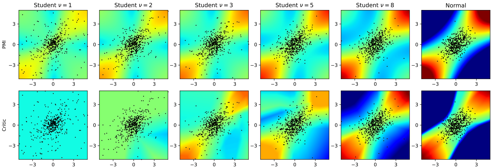
Qualitatively we see that the critic does not learn the correct PMI for , with better similarities for . For the normal distribution, the critic qualitatively approximates well the PMI function in the regions where the data points are available.
We hypothesise that these problems can be partly atributed to the longer tails of Student distributions (as the critic may be unable to extrapolate to the regions where few points are available) and partly to the analytical form of the PMI function — for the considered bivariate normal distribution the PMI is given by a simple quadratic function, which is not the case for the bivariate Student distribution.
E.2 Sample Size Requirements
We investigated the minimal number of samples needed to estimate the mutual information changing the number of samples in . We say that sample suffices to solve the task if for every the estimator provides the estimate between 2/3 and 3/2 of the ground-truth mutual information.
We present the minimal number of samples as a function of benchmark task and considered estimator in Fig. 9. Note that CCA and KSG typically need very small amount of samples to solve the task. As neural estimators use batch size of 256 and split the sample into training and test data sets, it is not possible for them to have , which is the smallest number of samples considered greater than .
E.3 Preprocessing
In Fig. 2 and Fig. 9 we transformed all samples by removing the mean and scaling by the standard deviation in each dimension calculated empirically from the sample. This strategy ensures that the scales on different axes are similar. Note that this strategy is not always suitable (e.g., if the distance metric used in the NN approach should weight select dimensions differently) and makes the observed data points not i.i.d. (as the “shared” information, sample mean and variances, has been used to rescale the variables), although the effect of it seems to be negligible on most tasks in the benchmark.
Additionally, we considered two other preprocessing strategies, implemented using the scikit-learn package [Pedregosa et al. 2011]: making each marginal distribution uniform by calculating empirical CDF along each axis (see Section D for the technical lemmata discussing this operation) and making each marginal distribution a Gaussian variable . These approaches may affect the effective sample size more strongly than the previous rescaling strategy, as estimating empirical CDF requires more data points than estimating mean and standard deviation.
We used data points and rerun the benchmark (see Fig. 10). Overall, the impact of the “uniformization” strategy appeared to be insubstantial for most tasks, and in certain cases negative. The “Gaussianisation” strategy improved estimation for Student distributions and helped histogram based approaches in low-dimensional tasks. Interestingly, both approaches worsen the performance of CCA on Student distributions.
While the improvements gained from “Gaussianisation” were minor, the approach is simplistic, treating each axis separately. Ideally, appropriate preprocessing would be able to transform into a better-behaved distribution , and thus simplify the estimation. In certain cases such preprocessing could (partially) undo transformations considered in our benchmark, and in effect make the estimators invariant (or more robust) to these transformations (cf. Section 4). We consider the design of informed preprocessing strategies an important open problem.
E.4 Hyperparameter Selection
CCA We used the implementation provided in the scikit-learn [Pedregosa et al. 2011] Python package (version 1.2.2). We set the latent space dimension to the smaller of the dimensions of the considered random vectors and .
Histograms Adaptive estimators such as JIC [Suzuki 2016] or MIIC [Cabeli et al. 2020] were not applicable to the high-dimensional data we considered, hence we resort to using an equal-width estimator implemented in TransferEntropy library (version 1.10.0). We fixed the number of bins to , although the optimal number of bins is likely to depend on the dimensionality of the problem.
KSG As a default, we used the KSG-1 variant from the rmi package with 10 neighbors. However, as shown in our ablation in Fig. 11, changing the number of neighbors or using the KSG-2 variant did not considerably change the estimates. We compared the used implementation with a custom Python implementation and one from TransferEntropy library. The version implemented in the TransferEntropy suffers from strong positive bias.
LNN We used the implementation from the rmi package (version 0.1.1) with neighbors and truncation parameter set to . Ablations can be seen in Fig. 11.
Neural Estimators We split the data set into two equal-sized parts (training and test) and optimized the statistics network on the training data set using the Adam optimiser with initial learning rate set to . We used batch size of 256 and ran each algorithm for up to training steps with early stopping (checked every 250 training steps). We returned the highest estimate on the test data set.
We chose the architecture using a mini-benchmark with four ReLU neural networks considered on two neural estimators (see Fig. 11) and chose a neural network with two hidden layers (network M in Table 2).
As neural estimators rely on stochastic gradient descent training, we implemented heuristic diagnostics used to diagnose potential problems with overfitting and non-convergence. We present the number of runs susceptible to these issues in Fig. 12. We did not include these runs when computing statistics in the main benchmark figures (Fig. 2 and Fig. 9).
| Architecture | Hidden layers |
|---|---|
| D | 8, 8, 8 |
| L | 24, 12 |
| M | 16, 8 |
| S | 10, 5 |
Appendix F Visualisation of Selected Tasks
In the following, we visualise a selection of benchmark tasks. Each figure visualises a sample of points from . The upper diagonal represents the scatter plots , and for all possible combinations of . The lower diagonal represents the empirical density fitted using a kernel density estimator with 5 levels. The diagonal represents the histograms of the marginal distributions and for all possible .
We present selected -dimensional tasks in Fig. 13 and Fig. 14; the -dimensional Swiss-roll distribution in Fig. 15 and selected -dimensional tasks in Fig. 16. Finally, in Fig. 17 we present two -dimensional problems, visualising the effect of the normal CDF and the spiral diffeomorphism.


Appendix G Author Contributions
Contributions according to the Contributor Roles Taxonomy:
- 1.
Conceptualization: PC, FG, AM, NB.
- 2.
Methodology: FG, PC.
- 3.
Software: PC, FG.
- 4.
Validation: FG, PC.
- 5.
Formal analysis: PC, FG.
- 6.
Investigation: FG, PC, AM.
- 7.
Resources: FG, NB.
- 8.
Data Curation: FG, PC.
- 9.
Visualization: FG, PC.
- 10.
Supervision: AM, NB.
- 11.
Writing – original draft: PC, AM, FG.
- 12.
Writing – review and editing: PC, AM, FG, NB, JEV.