Interpreting Deep Neural Networks with the Package \pkginnsight
Niklas Koenen, Marvin N. Wright
\PlaintitleInterpreting Deep Neural Networks with the Package innsight
\ShorttitleInterpreting DNNs with \pkginnsight
\AbstractThe \proglangR package \pkginnsight offers a general toolbox for revealing variable-wise interpretations of deep neural networks’ predictions with so-called feature attribution methods. Aside from the unified and user-friendly framework, the package stands out in three ways: It is generally the first \proglangR package implementing feature attribution methods for neural networks. Secondly, it operates independently of the deep learning library, allowing the interpretation of neural networks from any \proglangR package, including \pkgkeras, \pkgtorch, \pkgneuralnet, and even custom models. Despite its flexibility, \pkginnsight benefits internally from the \pkgtorch package’s fast and efficient array calculations, which builds on \pkgLibTorch – \pkgPyTorch’s \proglangC++ backend – without a \proglangPython dependency. Finally, it offers a variety of visualization tools for tabular, signal, image data, or a combination of these. Additionally, the plots can be rendered interactively using the \pkgplotly package.
\Keywordsneural networks, feature attribution, interpretable machine learning, explainable artificial intelligence, XAI, IML, \pkgtorch, \pkgkeras, \proglangR \Plainkeywordsneural networks, feature attribution, interpretable machine learning, explainable artificial intelligence, XAI, IML, torch, keras \AddressNiklas Koenen
Leibniz Institute for Prevention Research and Epidemiology – BIPS
Achterstr. 30
28359 Bremen, Germany
and
Faculty of Mathematics and Computer Science
University of Bremen
E-mail:
Marvin N. Wright
Leibniz Institute for Prevention Research and Epidemiology – BIPS
Achterstr. 30
28359 Bremen, Germany
and
Faculty of Mathematics and Computer Science
University of Bremen, Germany
and
Section of Biostatistics, Department of Public Health
University of Copenhagen, Denmark
E-mail:
1 Introduction
Throughout the past decade, neural networks have unleashed a tremendous surge of attention and infiltrated almost all conceivable domains of science, industry, and public life. Mainly, their increasing popularity is due to their natural ability to extract patterns and knowledge from vast amounts of structured raw data thanks to modern computing capacities and deliver outstanding performance (Krizhevsky et al. 2017; LeCun et al. 2015; Silver et al. 2016; Bengio et al. 2021). However, the intelligently learned decision-making process of a neural network remains inscrutable and hidden from the user due to its enormous complexity. Interpretations cannot be inferred as straightforward from this so-called black box as, for example, the coefficients of a linear model. As a consequence, the gain in predictive accuracy and model flexibility generally comes at the price of an increasingly opaque and intricate machine learning model, as was already noted by Gunning and Aha 2019. Nevertheless, it is precisely this question of interpretability – or, informally speaking: Why did a network make a certain prediction? – that is becoming more and more relevant for applications with high-stake decisions and possibly becoming a legal requirement, e.g., in autonomous systems (O’Sullivan et al. 2019), healthcare (Schneeberger et al. 2020) or data processing in general (European Union 2016; Goodman and Flaxman 2017).
Arising from this question and need, several methods have been proposed to explain predictions of machine learning models in a supervised learning setting. These methods are mainly classified according to the criteria for which model class they are applicable and at which level they provide explanations: Regarding the first criterion, model-agnostic approaches analyze the association of input data and model predictions of arbitrary models. Contrary, model-specific methods additionally exploit internal structures to reveal insights, but their application is restricted to a specific group of models. Secondly, interpretability methods for machine learning models can be categorized into local and global in terms of the explanation level. Established local model-agnostic methods, such as Shapley additive explanations (SHAP) (Lundberg and Lee 2017), individual conditional expectations (ICE) (Goldstein et al. 2015), and local interpretable model-agnostic explanations (LIME) (Ribeiro et al. 2016), explain only individual or groups of instances from the dataset, e.g., a single picture for image classification or one patient in the context of medical disease prediction. In contrast, global approaches describe the entire model behavior independent of individual effects. Commonly applied methods from this category are permutation feature importance (Fisher et al. 2019), accumulated local effect (ALE) plots (Apley and Zhu 2020) and partial dependence plots (Friedman 2001; Greenwell et al. 2018). One way to describe this distinction is to look at the classical linear model with input variables and prediction :
In this case, the coefficients describe the global effect of the input variables taking their values independent of , i.e., they indicate how much the variables affect the prediction in general. On the other hand, the local explanations demonstrate how much each input variable contributes to or impacts the prediction for a chosen input instance , commonly leading to a variable-wise decomposition of in additive effects.
Despite the quantity and universality of model-agnostic methods, they are barely applicable to modern deep neural networks mainly because of two reasons: Firstly, many of these model-agnostic approaches are based on repeated evaluation of perturbed or permuted input instances, and secondly, they scale poorly for a higher number of input variables. Since the forward pass of deep neural networks is computationally intensive and the inputs are often high-dimensional RGB images, applying model-agnostic approaches is time-consuming and challenging. Moreover, global variable-wise methods are generally not appropriate for image data since the importance of pixels is rather independent of the exact localization and depends more on the neighboring pixels varying in each individual image. Alternatively, global model-specific approaches such as feature visualizations (Olah et al. 2017) or concept-based methods (Kim et al. 2018) can only be used with further optimization procedures or concept-labeled datasets. This gap of interpretability methods for neural networks is being filled by feature attribution methods, which leverage all model-internal components in addition to the input and output relation, requiring only the model and the input instance to be explained. Particularly, this group of local model-specific methods, which assign relevance scores to each input variable for one of the output nodes or classes, prevailed and has successfully been applied in many domains (Zuallaert et al. 2018; Anders et al. 2019; Lauritsen et al. 2020). Furthermore, only a single regular forward pass and then a modified backward pass need to be performed for an explanation, i.e., they are generated without an optimization or estimation procedure. This two-step technique is illustrated in Figure 1: First, a prediction is produced in the standard forward pass, and the class to be explained is selected. In the subsequent method-specific backward pass, each input variable is assigned a relevance score to the chosen output class and can be visualized in a heat map or bar chart depending on the input type. An overview of the most popular feature attribution methods can be found in Section 2.
Several software packages have been developed in the last few years to make feature attribution methods widely accessible to users and to provide them with a unified and easy-to-use interface. The most popular packages are \pkginnvestigate (Alber et al. 2019) for the deep learning library \pkgKeras (Chollet et al. 2015), and \pkgcaptum (Kokhlikyan et al. 2020) and \pkgzennit (Anders et al. 2021) for \pkgPyTorch (Paszke et al. 2019). In addition, the \pkgshap package (Lundberg and Lee 2017) implements many Shapley-value-based methods and can handle both \pkgKeras and \pkgPyTorch models. However, all these packages are \proglangPython-exclusive and mostly only support networks of specific deep learning libraries. Despite the existing \proglangR packages for model-agnostic interpretability methods, such as \pkgiml and \pkgdalex (Molnar et al. 2018; Biecek 2018), we want to make feature attribution methods easily accessible to the \proglangR community and therefore provide the software package \pkginnsight, which pursues the following goals:
- •
First feature attribution \proglangR package: \pkginnsight is the first \proglangR package that implements the most popular feature attribution methods for neural networks unified in a single user-friendly package.
- •
Computationally efficient: The powerful \pkgtorch (Falbel and Luraschi 2023) package is utilized internally for all calculations, which builds on \pkgLibTorch, the \proglangC++ variant of \pkgPyTorch (Paszke et al. 2019), and doesn’t rely on a \proglangPython dependency.
- •
Deep-learning-library-agnostic: The passed trained models are not limited to a specific deep learning library. The package supports models from the \proglangR packages \pkgkeras (Kalinowski et al. 2023), \pkgtorch and \pkgneuralnet (Günther and Fritsch 2010). However, under some constraints, an arbitrary model can be passed as a list to be fully flexible.
- •
Visualization tools: \pkginnsight offers several visualization methods for individual or summarized results regardless of whether it is tabular, signal, image data, or a combination of these. Additionally, interactive plots can be created based on the \pkgplotly package (Sievert 2020).
The \pkginnsight package is available from the Comprehensive \proglangR Archive Network (CRAN) at https://CRAN.R-project.org/package=innsight or from our GitHub repository at https://github.com/bips-hb/innsight/.
The rest of the paper is structured as follows: First, we overview the most popular feature attribution methods for neural networks in Section 2. Then, in Section 3, we elaborate on the package’s design, functionality, and capabilities. Next, the package is applied to a basic example on a penguin dataset and an advanced example for melanoma detection based on image and tabular data as input types. In the concluding Section 5, the obtained package’s outputs are compared and validated with the already mentioned \proglangPython equivalents.
2 Methodology of feature attribution
Feature attribution methods for neural networks describe a group of local interpretation methods that assign to each input variable the contribution or impact to a chosen model output. For example, suppose an input instance with variables is fed forward through a neural network resulting in an output with classes or regression outputs. In this case, a feature attribution method assigns relevance scores to each of the input features of on a chosen output class or node of the prediction to be explained, as already described in Figure 1.
2.1 Gradient-based methods
Gradient-based methods are the fastest and most straightforward interpretation methods because they operate on the default techniques of the high-level deep learning libraries for computing gradients during the training loop. However, these methods – in a sense – calculate the derivatives of chosen output to the input variables instead of the derivatives of the loss value to the model parameters during gradient descent. Although the terminology of gradient-based methods can often be interpreted more broadly, we only consider techniques that use the default gradient methods. For example, Ancona et al. 2018 showed that variants of the layer-wise relevance propagation (LRP) and deep learning important features (DeepLift), discussed later in Section 2.2 and 2.3, can approximately be considered gradient-based. Regardless, they are not mentioned in this section, since not all LRP and DeepLift variants can be considered gradient-based. Additionally, these variants require an overwriting of the standard gradients, i.e., they don’t use the mathematical definition of the gradient anymore. In the following, the most common gradient-based feature attribution methods are briefly explained, including their underlying objectives. For a more mathematical overview, see Figure 2.
One of the first and most intuitive methods for interpreting neural networks is the Gradient method introduced by Simonyan et al. 2014, also known as Vanilla Gradients or Saliency maps. This method computes the gradients of the selected output with respect to the input variables. Therefore, the resulting relevance values indicate prediction-sensitive variables that can be locally perturbed the least to change the outcome the most. Assuming that the model behaves linearly overall, increasing by one raises the output by the calculated gradient. In general, neural networks are highly nonlinear, which forces the gradients to have large fluctuations or abrupt changes. This phenomenon can introduce noise and potential misinterpretations in the Gradient method. A simple extension of this basic Gradient method to tackle this issue is the smoothed gradients (SmoothGrad) approach introduced by Smilkov et al. 2017. They proposed computing the gradients of randomly Gaussian perturbed copies of and determining the average gradient from that, instead of calculating only the gradient in . As a result, locally very noisy gradients are smoothed out and the method provides the average behavior in a larger neighborhood of . The estimation accuracy and size of the neighborhood can be adjusted with the hyperparameters for the number of perturbations and for the variance of the Gaussian noise. With the value of , the estimation accuracy for the average gradient can be increased, but this goes hand in hand with a higher computational effort. The second parameter is mostly specified indirectly via a noise level determining the proportion of the total range of the input domain that is covered by the standard deviation , i.e., . Especially for images, this argument can be used to control the visual smoothness of the explanation.
A simple modification can change both previously discussed methods to the methods GradientInput and SmoothGradInput. The gradients are calculated as for the respective methods and then multiplied by the corresponding feature values. The GradientInput method was introduced by Shrikumar et al. 2017b and relies on a well-grounded mathematical background despite its simple idea: The basic concept is decomposing the output prediction according to its relevance to each input variable , i.e., into variable-wise additive effects
| (1) |
Mathematically, this method is based on the first-order Taylor decomposition. Assuming that a function is continuously differentiable in , a remainder term with exists such that
The first-order Taylor formula thus describes a linear approximation of the function at the point since only the first derivatives are considered. Consequently, a highly nonlinear and continuous function is well approximated only in a small neighborhood around . For larger distances from , sufficient small values of the residual term are not guaranteed anymore. The GradientInput method considers the data point and sets . In addition, the residual term and the summand are ignored. Analogously, this multiplication can be applied to all gradients in the summation of the SmoothGrad method in order to compensate for local fluctuations.
Even though the multiplication of gradients by the inputs provides an approximate decomposition of , this approach only captures the feature-wise effects of concerning a baseline of . However, this value does not necessarily reflect a prediction-neutral reference value and can be challenging to interpret or even lie outside the data distribution. Sundararajan et al. 2017 proposed a method called IntegratedGradient as a way to find a decomposition of into feature-wise effects for an arbitrary reference value , using integration over the GradientInput values along an integration path. In practice, the integral is approximated by the sum of gradients multiplied by the inputs along an interpolated path from to . Nevertheless, choosing the reference value remains a challenging task and ideally requires domain-specific knowledge. The ExpectedGradient method (Lundberg and Lee 2017; Erion et al. 2021) addresses this issue by estimating the mean value of the IntegratedGradient method through Monte Carlo integration, considering the whole distribution of reference values instead of a single baseline. In this sense, the method finds a feature-wise decomposition of and, thus, calculates approximately Shapley values.
2.2 Layer-wise relevance propagation (LRP)
The layer-wise relevance propagation (LRP) method was introduced by Bach et al. 2015 and has a similar goal as the GradientInput approach explained in the previous section: decomposing the output into variable-wise relevances conforming to Equation 1. The distinguishing aspect is that the prediction is redistributed layer by layer from the output node back to the inputs according to the layer’s weights and intermediate values. The entire procedure is accomplished by rule-based relevance messages defining how to redistribute the upper-layer relevance to the lower layer. A high-level overview of this method applied to a neural network with layers can be seen in Figure 3(a). The method mainly consists of the following iterative steps: As the starting point, the relevance for the considered output node is set to the respective prediction score . Subsequently, the relevance of the lower layer’s node is calculated using the sum of all incoming relevance messages. A relevance message describes the proportion of the upper-layer relevance that is sent to a node in the lower layer. This process is repeated layer by layer backwards, as shown in Figure 3(a), until the input layer is reached and relevances are obtained for each input feature. More precisely, for a hidden layer , the relevance message from node in the upper layer to node in the preceding layer defines the proportion of the relevance from attributed to the node in the lower layer. Since the relevance messages are based solely on the contribution from a single upper-layer node, the overall relevance of the node is obtained by summing up all incoming relevance messages (see Figure 3(b)), i.e.,
| (2) |
Since the publication of the LRP method, various variations of relevance messages flowing from the upper layer to the lower-layer node have emerged. However, the fundamental rule on which all other variations of relevance messages are more or less based is the simple rule (also known as LRP-0). The relevances are redistributed to the lower layers according to the ratio between local and global pre-activation. Despite being a rule-based approach, if the neural network only includes ReLU activations, this rule makes the method LRP equivalent to GradientInput presented in Section 2.1 (Ancona et al. 2018). Let be the input, the weight matrix and the bias vector of layer , and the upper-layer relevance; then is the local and the global pre-activation defining the simple rule as (also used in Fig. 3(b))
| (3) |
Many other rules for relevance messages are built upon this principle. The well-known variations -rule and --rule of the simple rule and their advantages and disadvantages are explained in the Appendix A.1. Additionally, a brief summary of other rules discussed in the literature is provided there.
2.3 Deep learning important features (DeepLift)
One method that, to some extent, echoes the idea of LRP is the so-called deep learning important features (DeepLift) method introduced by Shrikumar et al. 2017a. It behaves similarly to LRP in a layer-by-layer backpropagation fashion from a selected output node back to the input variables, considering the simple rule. However, it incorporates a reference value to compare the relevances with each other, analogously to the IntegratedGradient method discussed in Section 2.1. Hence, the relevances of DeepLift represent the relative effect of the outputs of the instance to be explained and the output of the reference value . By taking the difference, the bias term is eliminated in the relevance messages, preventing the relevance absorption and leading to an exact variable-wise decomposition of the difference-from-reference output , i.e.,
Similar to the relevance messages for LRP, DeepLift defines so-called multipliers for each layer or part of a layer. Based on these multipliers, the contribution of an arbitrary input (or intermediate) variable to the difference-from-reference output can be obtained by multiplying it by the corresponding difference-from-reference value. For an arbitrary layer with the layer’s input , reference input , and multiplier , this means:
| (4) |
The multipliers fulfill a chain rule allowing the computation of the multiplier for the preceding layer given the already calculated one , i.e.,
| (5) |
In other words, the chain rule justifies defining the multipliers for each layer or part of a layer separately before combining them with the upper-layer multipliers. For linear components, such as the matrix multiplication in dense or convolutional layers, the weights are used as the multipliers, i.e., . For nonlinear components, like, e.g., all point-wise activations such as ReLU, tanh, or sigmoid, Shrikumar et al. 2017a propose the Rescale and RevealCancel rule. While the Rescale rule uses the ratio of the layer’s difference-from-reference output and difference-from-reference pre-activation as the multiplier, the RevealCancel rule is designed to propagate meaningful relevances even for saturated activations and discontinuous gradients through the layers’ activation part. For a more detailed explanation, we refer to the Appendix A.2. These rules, along with the chain rule (Eq. 4-5), enable the successive computation of the input variables’ contributions to the difference-from-reference output in a single backward pass.
The reference value is the only crucial hyperparameter for the DeepLift method, apart from the rule for non-linearities. This choice depends significantly on the application and usually requires proficient domain-specific knowledge. Nevertheless, the authors suggest asking oneself the question of what one wants to measure an effect against. For example, taking the background color or blurred versions of the original picture as the reference values for images are reasonable choices. In many cases, zeros as a baseline are also used. Ancona et al. 2018 showed that using the Rescale rule with activations crossing the origin (i.e., ) and a zero baseline as reference value coincides with the GradientInput method discussed in Section 2.1 and with LRP with the simple rule. Similar to how the ExpectedGradient method generalizes IntegratedGradient considering the distribution of baseline values instead of a single reference value, the DeepSHAP (Lundberg and Lee 2017) method extends the DeepLift technique. It calculates the average DeepLift value across various baseline values, thereby achieving a decomposition of into feature-wise effects and, thus, gives approximately Shapley values.
2.4 Connection weights
One of the earliest methods specifically designed for neural networks is the connection weights (CW) method invented by Olden et al. 2004, resulting in a global relevance score for each input variable. The basic idea of this approach is to multiply all path weights for each possible connection between an input variable and the output node or class and then calculate the sum of all of them. However, this method ignores all bias vectors and all activation functions during calculation. Analogously to the previous methods, CW can also be defined layer by layer, deriving the relevance for layer from the upper layer as follows:
Since only the model weights are used, this method is independent of input data and, thus, a global interpretation method. Inspired by the method GradientInput, it can also be extended into a local method by taking the point-wise product of the global CW method and the input data.
2.5 Choice of the method
Overall, the choice of methods for a user remains an open research question, but there are several recommendations that can be derived from the complexity or stated goals of the methods. Firstly, consider the computational efficiency of the method. Standard gradient methods such as Gradient and GradientInput, as well as LRP, are very fast but can be very noisy as they only examine a very local behavior. On the other hand, methods like SmoothGrad, IntegratedGradient, and ExpectedGradient often require a high number of forward passes to deliver accurate results, but also consider the local neighborhood or baseline values. Furthermore, it has been demonstrated that many methods (such as GradientInput, LRP, IntegratedGradient, DeepLift) are not invariant to constant shifts of the inputs (Kindermans et al. 2019; Haug et al. 2022; Nielsen et al. 2022). This is because the Taylor approximation is only accurate around zero (or the reference value), and the choice of the reference value has a crucial impact. One solution to this is provided by Shapley-based methods like ExpectedGradient and DeepSHAP. However, these methods require a highly informative reference dataset in addition to the instance to be explained, and they are noticeably slower. These considerations highlight the trade-offs involved in selecting a feature attribution method for a given task, and it is crucial for users to weigh the speed, accuracy, and invariance characteristics based on the specific requirements of their application.
3 Functionality and usage
The \proglangR package \pkginnsight combines all the methods discussed in the previous section in a user-friendly structure and a unified step-based workflow from the trained model to the visualization of the relevances of a feature attribution method. For efficient high-dimensional array calculations, the package utilizes the \proglangR package \pkgtorch (Falbel and Luraschi 2023), which builds on \pkgLibTorch (the \proglangC++ variant of \pkgPyTorch (Paszke et al. 2019)), and consequently runs without a \proglangPython dependency (see Fig. 4). The following three steps yield the requested results, regardless of the class of the passed model or the chosen feature attribution method:
- -
Step 1: Convert the model
- -
Step 2: Apply selected method
- -
Step 3: Get or visualize results.
Internally, a class structure is being built using \codeR6 classes based on the equally named package \pkgR6 (Chang 2021). This type of object-oriented programming class is used because \pkgtorch also relies on it, and it simplifies inheritance and argument passing compared to conventional \codeS3 and \codeS4 classes. Apart from the utilized packages for the internal workflows, calculations, and visualizations discussed in the following sections, the packages \pkgcheckmate (Lang 2017) and \pkgcli (Csárdi 2023) are generally used for all argument verifications, internal checks, and terminal outputs of messages, warnings, and errors.
For illustration and better comprehension, the three steps will be exemplified from a user’s perspective using the bike sharing dataset (Fanaee-T 2013). The internal mechanisms and more detailed descriptions are provided in the subsequent sections. This regression dataset contains information about the number of bicycles rented on a given day, along with various features such as weather conditions, holidays, and temperature. When using the \pkginnsight package, object-oriented \codeR6 objects are internally created at each step, but their initialization is simplified through function calls providing a conventional \proglangR usage without prior knowledge about \codeR6 classes. This facilitates easy application for \proglangR users of the package.
In the following code snippet, the dataset is loaded and restricted to a few variables. The outcome in this regression dataset is \code"cnt", indicating the total number of bicycles rented on the given day. The model is trained on this dataset using the \pkgneuralnet package (Günther and Fritsch 2010) containing one hidden layer with neurons. In addition, the outcome variable \code"cnt" is scaled to bikes per . {CodeInput} R> library("neuralnet") R> set.seed(42) R> bike <- read.csv("additional_files/bike_sharing/day.csv") R> bike <- bike[, c("cnt", "holiday", "workingday", + "temp", "hum", "windspeed")] R> bikecnt / 10000 R> bike <- as.matrix(bike) R> model <- neuralnet(cnt ., data = bike, hidden = c(64), + linear.output = TRUE)
To enable a deep-learning-library-agnostic implementation, the given model \codemodel is analyzed in the first step, and internally, a replica based on the \pkgtorch package is reconstructed. However, for the user, this process is abstracted through the \codeconvert() function, allowing the adjustment of the used variable and outcome names, e.g., with the argument \codeoutput_names: {CodeInput} R> library("innsight") R> conv <- convert(model, output_names = c("Number of rented bikes/10,000"))
In the second step, the user’s method of choice can be applied to the provided data (argument \codedata). Internally, an \codeR6 class for the respective method is initialized but hidden from the user again. In this case, the DeepSHAP method (\coderun_deepshap()) is run on the first instances with the entire dataset as reference values. For computational reasons, the internal calculation uses samples from this dataset, as this is the default value of \codelimit_ref. In addition, the data must always be passed as input data only, which is why the outcome variable \code"cnt" is removed in the following code: {CodeInput} R> res_deepshap <- run_deepshap(conv, bike[1:20, -1], data_ref = bike[, -1])
In the final step, results can be extracted, for instance, using the \codeget_result() function, or visualized using \codeplot() or \codeplot_global()/\codeboxplot(). The \codeboxplot() method is an alias for \codeplot_global() in case of tabular and signal data, as boxplots are created for these data types. It is noted that the variable \code"hum" for humidity is scaled between and , and \code"tmp" and \code"windspeed" are divided by the respective maximal value, i.e., and . The visualization relies on the \pkgggplot2 package and can be customized accordingly (the plots are shown in Fig 5(a)): {CodeInput} R> library("ggplot2") R> head(get_result(res_deepshap)) R> plot(res_deepshap) R> boxplot(res_deepshap, ref_data_idx = 1) + + theme(text = element_text(face = "bold")) {CodeOutput} , , Number of rented bikes/10,000
holiday workingday temp hum windspeed [1,] 0.004659358 0.050143935 -0.1218946 -0.08540524 0.0109126559 [2,] 0.007893519 0.064216673 -0.1305959 -0.01469872 -0.0320372544 [3,] -0.009826845 0.007002956 -0.2871930 0.09675989 -0.0359177366 [4,] -0.011643781 0.028260766 -0.2517902 0.04398110 0.0213681515 [5,] -0.009875727 0.015752951 -0.2339799 0.09297864 -0.0008396581 [6,] 0.002854239 -0.004088928 -0.2964459 0.05857125 0.0088869939
For example, in the box plots (see Fig. 5(a) bottom), bold font is used for the labels, which is achieved through the \codetheme(text = element_text(face = "bold")) feature of \pkgggplot2. By default, the orientation of relevances is concealed by absolute values, as global attention is usually focused on the strength of the effects. Consequently, it can be observed that the model considers temperature as the most crucial feature for its predictions. Furthermore, the argument \coderef_data_idx is employed to highlight the relevances of the first instance of the dataset as a reference value with red lines. This instance and its local effects are more precisely visualized in the upper illustration of Figure 5(a). It also shows that temperature is an influential factor for the model since it predicts a relatively low count of bicycles (compared to the average of bicycles). This aligns with the data, as on that particular day, the temperature is °C (normalized value ), while the dataset’s average temperature is °C (normalized value ). Additionally, the plot includes a small box displaying the model’s prediction of the instance (), the sum of calculated relevances (), and the decomposition target of the method (). For example, the DeepSHAP method is based on the decomposition of the difference between the prediction and the average prediction in the baseline dataset (i.e., ), which is for the first instance , i.e., bikes below the average.
3.1 Step 1 - Convert the model
The key step that turns the \pkginnsight package into a deep-learning-library-agnostic approach and unlocks the provided \pkgtorch toolbox to all methods is this first step, which essentially analyzes a passed model and creates a \pkgtorch-based replication. For the user, however, the internal processes remain hidden, and the entire conversion step is accomplished by creating a new instance of the class \codeConverter: {Code} Converter
3.2 Step 2 - Apply selected method
As previously mentioned, the \pkginnsight package provides the most popular feature attribution techniques in a unified framework. For package users, simple functions are provided to apply the respective method to the data, as demonstrated at the beginning of this section with the bike sharing dataset using the \coderun_deepshap() function. However, before delving into the individual user-facing functions, their internal class-related origin is explained, since the fundamental structure of the methods remains consistent. Internally, the unification is achieved by the \codeR6 super class \codeInterpretingMethod, from which all methods intended for users inherit and only add method-specific arguments to those of the super class. The rudimentary call of initializing a new method object looks like this: {Code} InterpretingMethod
3.3 Step 3 - Get and visualize the results
After creating an object of a selected method, in the third step the results can be extracted or, if required, presented in a descriptive and visual way. For this purpose, the \pkginnsight package provides three generic methods \codeget_result(), \codeplot() and \codeplot_global() that either return the results as an \proglangR object (such as \codearray, \codetorch_tensor or \codedata.frame) or create visualizations for individual instances or aggregated results over the whole passed dataset. All three generic functions call the respective class methods in the \codeInterpretingMethod super class, which are inherited by all the interpreting methods from the second step by design. For instance, in the bike sharing example from the section’s beginning, the plot is generated using \codeplot(res_deepshap) instead of \coderes_deepshap
3.3.1 Generic function \codeget_result()
The function \codeget_result() can be used to obtain the results in various forms, whatever is favored according to the user’s subsequent workflow or application. This method has only the argument \codetype (besides the method object), which determines the representation of the returned results. By default (\codetype = "array"), the result is returned as an \proglangR base \codearray, including the input and output names in the corresponding dimensions specified in the first step in the \codeConverter object (see Sec. 3.1). The shape of the array is composed of the input shape including the batch size and the number of computed output nodes, i.e., for a tabular input with ten instances and four input variables, the shape is if the method was applied to three output nodes in Step 2. In the example with the bike sharing dataset, an array of size was returned using \codeget_result(res_deepshap) which also includes the class label \code"Number of rented bikes/10,000". This is because instances were explained, and the model has features and one output node. In the same way, \codetype = "torch_tensor" returns a \codetorch_tensor object having the same shape as the array, but without dimension labels. However, both variants can also return a list or list of lists with the related results as an \codearray or \codetorch_tensor for models with multiple input or output layers. The third and last format of the results is an \proglangR base \codedata.frame obtained with \codetype = "data.frame". Included are columns for the input instance (\code"data"), the input and output layer of the model (\code"model_input" and \code"model_output"), the input variable (\code"feature") – possibly also a second one for images (\code"feature_2") and the channel for signal and image data (\code"channel") – the output node or class (\code"output_node"), and the relevance (\code"value") for the corresponding values. Moreover, the generated \codedata.frame contains variables that show the prediction of the instance or already aggregated relevances for the respective output node and instance. The column \codedecomp_goal indicates the decomposition goal of the method aimed by the aggregated relevances explained in Section 2, e.g., for the DeepSHAP method.
3.3.2 Generic function \codeplot()
The generic function \codeplot() visualizes individual instances of the result of the method applied before based on the graphic package \pkgggplot2 (Wickham 2016) or the package \pkgplotly (Sievert 2020) for interactive graphics if the corresponding argument \codeas_plotly is set. The call for a method’s object \codemethod is executed as follows: {Code} plot(method, data_idx = 1, output_idx = NULL, output_label = NULL, aggr_channels = "sum", as_plotly = FALSE, same_scale = FALSE, show_preds = TRUE) The key arguments are \codedata_idx and \codeoutput_idx/\codeoutput_label, which specify the indices for the dataset instances and the indices/labels for the desired output nodes or classes whose result is to be visualized. By default, the first data instance and the first computed output node are used. In the argument \codeoutput_idx, no arbitrary indices can be passed, but only those for which the results were calculated previously in the second step. The same applies to \codeoutput_label, which must additionally be a subset of the output names \codeoutput_names in the \codeConverter object. The further argument \codeaggr_channels can be used to define how the channels are aggregated for image and signal data. There are various options for choosing this aggregation function, which may significantly influence the quality of the explanation (Arras et al. 2022). Nevertheless, for \pkginnsight, the default is to compute the sum over the channels, which aligns with the additivity axiom for Shapley values to accurately reflect the collective group effect (Strumbelj and Kononenko 2010). Since visualization depends on the data type, it is internally distinguished between tabular/signal data and image data; accordingly, a bar chart or a raster chart is created, as shown in Figure 6 on the left. The relevances in the bars or the pixels are also scaled by color, facilitating a visual comparison; red means positive, blue negative, and white the absence of relevance. Since, in general, the scales vary significantly for the selected output class or data instance, the plots are scaled separately for each value in \codeoutput_idx/\codeoutput_label and \codedata_idx. When several input layers are to be visualized, the remaining argument \codesame_scale can be used to select whether the individual input layers are also scaled separately in terms of color. This decision depends on the use case, as illustrated in the melanoma example in Section 4.2. Additionally, in each plot, a small box displaying information for the respective instance and output node is presented. This includes the prediction, the sum of relevances, and, if available, the method’s decomposition target of the sum of relevance. The appearance of the box can be toggled with the \codeshow_preds argument. For the bike rental example, Figure 5(a) top shows the visualized relevances of the first instance and the box with the additional predictive and decomposition information. Furthermore, instead of returning objects from the \pkgggplot2 or \pkgplotly packages, instances of the \codeS4 classes \codeinnsight_ggplot2 and \codeinnsight_plotly are produced, which are explained in the Appendix C for advanced visualizations.
3.3.3 Generic function \codeplot_global()
Global behavioral patterns and insights into the model’s decision-making process can be derived from the results of multiple instances by appropriately summarizing and aggregating them. The generic function \codeplot_global() visualizes these global interpretations over the whole or parts of the given dataset based on the graphics package \pkgggplot2 (Wickham 2016) or the package \pkgplotly (Sievert 2020) for interactive charts analogous to the previously discussed function \codeplot(). Box plots are created for the features of tabular and signal data, and the median pixels’ relevance is shown for image data due to the high dimensionality. For the former, the alias function \codeboxplot() can also be used analogously. The call for a method’s object \codemethod is the following:
plot_global(method, output_idx = NULL, output_label = NULL, data_idx = "all", ref_data_idx = NULL, aggr_channels = "sum", preprocess_FUN = abs, as_plotly = FALSE, same_scale = FALSE, …) # For tabular and signal data boxplot(method, …) In addition to the identical arguments \codeoutput_idx/\codeoutput_label, \codeaggr_channels,\codeas_plotly, and \codesame_scale for the \codeplot() function, options for selecting the data points to be aggregated (\codedata_idx), for drawing a reference data point (\coderef_data_idx) and a pre-process function of the results (\codepreprocess_FUN) are added. By default, the absolute values of the relevances are calculated, as in global contexts, the focus is usually more on the intensity of effects rather than their orientation. However, this can be adjusted with the \codepreprocess_FUN argument, e.g., showing the orientation with \codeidentity. Analogous to \codeplot(), the visualization style depends on the type of input data; tabular and signal data are displayed as box plots, whereas only a raster plot with the pixel-wise median is rendered for image data due to the high dimensionality. For example, a box plot is created in the bike sharing example since it contains tabular data (see Fig. 5(a) bottom). In this visualization, the red reference lines are drawn for the first dataset instance using the argument \coderef_data_ix. However, if the chart is \pkgplotly-based, there is a slider to select which quantile to display. Basic examples and an overview of the \codeplot_global() function are given in Figure 6 on the right. Despite the creation of \pkgggplot2 or \pkgplotly graphs, instances of the \codeS4 class \codeinnsight_ggplot2 or \codeinnsight_plotly are returned, which are explained in the Appendix C.
4 Illustrations
To exemplify the methods and step-by-step execution of the \pkginnsight package, a standard dataset with only numerical tabular inputs on a simple model and a more complex dataset with image and tabular data on an extensive non-sequential network are analyzed in the following. The penguin dataset from the \pkgpalmerpenguins package (Horst et al. 2020) is used as the simple dataset, taking only the numerical variables of bill length and depth, flipper length, and body weight as inputs. The melanoma dataset (Rotemberg et al. 2020) of the Kaggle competition11 1 See the following link for the official dataset description https://www.kaggle.com/competitions/siim-isic-melanoma-classification/overview/description is taken as the second dataset, which classifies the malignancy or benignity of the skin cell based on images of skin lesions and moles, and patient-level contextual information. Both datasets are classification tasks. Even though the bike sharing dataset has already exemplified a regression problem, feature attribution methods typically treat classification problems similarly to regression problems: The activation of the last layer – usually sigmoid or softmax functions – is ignored, and the pre-activation score is explained instead of the actual probability (Shrikumar et al. 2017a; Montavon et al. 2019).
4.1 Example 1: Penguin dataset
In the first example, the penguin dataset provided by the \pkgpalmerpenguins package (Horst et al. 2020) is used, and a neural network consisting of a dense layer is trained using the \pkgneuralnet package (Günther and Fritsch 2010). Before the \pkginnsight package can be applied, the dataset must be processed, and the neural network must be trained on the modified dataset. As a first pre-processing step, only the variables with the species, bill length and depth, flipper length, and body weight are selected, cleaned of missing values, and numerical variables are normalized: {CodeChunk} {CodeInput} R> library("palmerpenguins") R> set.seed(42) R> data <- na.omit(penguins[, c(1, 3, 4, 5, 6)]) R> data[, 2:5] <- scale(data[, 2:5]) Next, the dataset is divided into training data and test data at a ratio of to : {CodeChunk} {CodeInput} R> train_idx <- sample.int(nrow(data), as.integer(nrow(data) * 0.75)) R> train_data <- data[train_idx, ] R> test_data <- data[-train_idx, -1] In the second pre-processing step, a network with units in a single hidden layer and the logistic function as activation is fitted on the training data \codetrain_data: {CodeChunk} {CodeInput} R> library("neuralnet") R> model <- neuralnet(species ., data = train_data, hidden = 128, + act.fct = "logistic", err.fct = "ce", linear.output = FALSE) Now, we follow the three steps that provide and visualize an explanation of the model \codemodel on the test data \codetest_data, which were described in detail in Section 3. As a reminder, the first step uses the \codeconvert() – a shortcut function for initializing an object of the \codeR6 class \codeConverter – to convert the given \codemodel to a \pkgtorch-based model: {CodeChunk} {CodeInput} R> library("innsight") R> conv <- convert(model) Then, in the second step, the desired method is selected and applied to the test data \codetest_data via the corresponding function \coderun_* which is identical to initializing the respective \codeR6 class. In this example, the IntegratedGradient method is applied with the average feature value as a baseline: {CodeChunk} {CodeInput} R> intgrad <- run_intgrad(conv, test_data, + x_ref = matrix(colMeans(test_data), 1))
In the last step, the results are visualized in two ways: Using the \codeplot() function, the relevances of one instance of the species Adelie (data index ) and one of the species Gentoo (data index ) are displayed for both corresponding classes. Secondly, the results for the two classes, Adelie and Gentoo, are aggregated over the entire test data, and box plots are generated using the \codeboxplot() function, showing the first penguin as a reference. As mentioned in Section 3, these two variants can be treated and modified like ordinary \pkgggplot2 objects, e.g., adding themes or rotating the x-axis labels. Both visualizations are executed by the following code and can be viewed in Figure 7: {CodeChunk} {CodeInput} R> library("ggplot2") R> plot(intgrad, data_idx = c(1, 50), output_label = c("Adelie", "Gentoo")) + + theme_bw() + + theme(axis.text.x = element_text(angle = 45, vjust = 0.6)) R> boxplot(intgrad, output_label = c("Adelie", "Gentoo"), ref_data_idx = 1) + + theme_bw() + + theme(axis.text.x = element_text(angle = 45, vjust = 0.6)) In Figure 7(a), it can be seen that the bill length for the chosen penguin of the Adelie class (index in the dataset \codetest_data) is highly relevant – based on the trained model – for this particular class aligning to the prediction of which is shown in the info box. At the same time, the penguin’s flipper length argues against the Gentoo class due to its strong negative relevance. For the Gentoo penguin, the bottom row in Figure 7(a) reveals that the bill depth is decisively in favor of the Gentoo class and concurrently against the Adelie species. The respective info boxes show that the model is generally very confident in its prediction and that the method has achieved its decomposition goal very well. As mentioned at the beginning of the section, the pre-activations are decomposed by default for classification problems and not the probability scores. Besides these instance-wise explanations, the \codeboxplot() function provides aggregate insights across the entire test data \codetest_data, summarized in Figure 7(b). The box plots show that, indeed, the bill length and depth are the most crucial variables for the Adelie class and consequently strongly influence it. Simultaneously, however, the length of the bill is not as decisive for the Gentoo class, but the bill depth is. It further emerges that the flipper length is another crucial feature for the Gentoo class. The red lines for the first penguin also show that the bill depth is not as relevant as it is on a global scale.
4.2 Example 2: Melanoma dataset
The second example examines the melanoma dataset (Rotemberg et al. 2020) from the Kaggle challenge22 2 See the following link for the official dataset description https://www.kaggle.com/competitions/siim-isic-melanoma-classification/overview/description in 2020, issued by the society of imaging informatics in medicine (SIIM) and based on the international skin imaging collaboration (ISIC) archive, the most extensive publicly available collection of quality-controlled dermoscopic images of skin lesions. This dataset consists of labeled images with associated patient-level contextual information, such as the age, gender, and image location of the skin lesion or mole.
Due to the complexity and high dimensionality of the data, training a neural network is not straightforward and overall not the main focus of this paper thus, reference is made to the GitHub repository for reproduction (https://github.com/bips-hb/JSS_innsight/), and only the most notable points are summarized in the following: The tabular input part’s numerical and one-hot encoded categorical variables are fed into a sequential model of dense layers. On the other hand, an architecture based on the established residual layers (He et al. 2016) considering skip connections between convolutional layers is used for the image data. Afterward, the two outputs of the respective input parts are merged by concatenation and finally flow in a sequential model with only dense layers to obtain a prediction probability for the skin lesion status. The coarse structure is summarized in Figure 8, where additional dropout layers are used between dense layers. Furthermore, the numerical variable age and the one-hot encoded variables gender and location yield ten features as inputs for the tabular model, and the images are resized to for the image model. This model architecture is trained on the melanoma dataset with a validation split of and a batch size of instances using the \pkgKeras library (Chollet et al. 2015) with stochastic gradient descent as the optimizer and class-weighted binary cross-entropy as the loss function. The best model is selected based on the highest value of the area under the ROC curve (AUC) on the validation data. This metric is chosen because the dataset is highly imbalanced with only of the images containing a malignant skin lesion. Since the model is trained from scratch and the image model has significantly more parameters than the tabular one, training starts with warm-up epochs on the image model using the image data only. Then, the image model is joined with the tabular and the dense output model. Afterward, training continues on the image and tabular data, saving the model with the highest value of the AUC metric on the validation data. In addition, the initial learning rate of is reduced by a factor of after epochs without a validation AUC improvement, and training is terminated after unimproved epochs. With this approach, an AUC value of and an accuracy of on the validation data are achieved, and the model to be interpreted is selected.
Based on this model, the obtained predictions can now be explained using the 3-step approach of \pkginnsight: In the first step, the trained model is loaded and converted to a \pkgtorch-based model using the \codeconvert() function for initializing a \codeConverter object. However, since \pkgkeras models do not include names of the input variables and output nodes, these can be passed along when initializing the converter to preserve meaningful labels of the input and output variables in the visualizations. Thus, the first step is executed by the following \proglangR code:
R> library("keras") R> library("innsight") R> model <- load_model_tf("additional_files/melanoma_model.h5") R> input_names <- list( + list(paste0("C", 1:3), paste0("H", 1:224), paste0("W", 1:224)), + list(c("Sex: Male", "Sex: Female", "Age", + "Loc: Head/neck", "Loc: Torso", "Loc: Upper extrm.", + "Loc: Lower extrem.", "Loc: Palms/soles", "Loc: Oral/genital", + "Loc: Missing"))) R> output_name <- c("Probability of malignant lesion") R> converter <- convert(model, input_names = input_names, + output_names = output_name) Next, the LRP method with composite rules is applied, which selects the propagation rule depending on the layer type. For convolutional layers, the --rule with is used to favor the positive over the negative relevances. In addition, the -rule with is performed on all dense layers and the simple rule – the rule used by default – on average pooling layers. This second step is performed with \pkginnsight as follows: {CodeChunk} {CodeInput} R> rule_name <- list(Conv2D_Layer = "alpha_beta", Dense_Layer = "epsilon") R> rule_param <- list(Conv2D_Layer = 1.5, Dense_Layer = 0.01) R> res <- run_lrp(converter, inputs, channels_first = FALSE, + rule_name = rule_name, rule_param = rule_param) For the sake of simplicity, the loading of the input data \codeinputs is omitted in the above code snippet and can be found in the reproduction material together with the whole example. In addition, the channel axis of the images is located at the last position, which is why the argument \codechannels_first must be set to \codeFALSE. The results can be visualized using the implemented \codeplot() function. By default, the results are scaled using colors (red for positive and blue for negative relevances) for each instance, each considered output node and each input layer individually. This behavior is especially appropriate for models with multiple input layers consisting of images mixed with tabular data. Because even if the relevances are the same at the end of the tabular and image model before merging, they are further propagated to only ten input variables for the tabular and variables for the image model, leading to potentially different relevance scales. The following code produces the plot object based on the \codeS4 class \codeinnsight_ggplot2 for the first three dataset instances, which can be treated as a \pkgggplot2 object (see Appendix C for details): {CodeChunk} {CodeInput} R> library("ggplot2") R> p <- plot(res, data_idx = 1:3) + theme_bw() Since this model has no standard architecture and the visualization is more extensive, the suggested packages \pkggridExtra (Auguie 2017) and \pkggtable (Wickham and Pedersen 2023) are required. However, each individual plot in the object \codep can now be modified individually based on the \pkgggplot2 syntax. The indexing works as the objects are plotted in a matrix-wise fashion, provided by the facet rows and columns. It is pointed out that each plot object is based on the same dataset, which is also created by the method \codeget_result(type = "data.frame"), i.e., the same column names can be used within the \pkgggplot2 syntax. In the following code snippet, the facet and the x-axis labels are changed manually, and the plot is visualized, which can be found in Figure 9: {CodeChunk} {CodeInput} R> p[1, 1] <- p[1, 1, restyle = FALSE] + + facet_grid(cols = vars(model_input), + labeller = as_labeller(c(Input_1 = "Image input"))) R> p[1, 2] <- p[1, 2, restyle = FALSE] + + facet_grid(cols = vars(model_input), rows = vars(data), + labeller = as_labeller(c(Input_2 = "Tabular input", + data_1 = "malignant"))) R> p <- p + theme(axis.text.x = element_text(angle = 45, vjust = 0.6)) R> plot(p, heights = c(0.31, 0.31, 0.38)) The argument \coderestyle is set when indexing the \codeinnsight_ggplot2 object, ensuring that the subplots are extracted in the same way as they are displayed in the whole plot. Otherwise, the entire plot’s corresponding facet stripes and axis labels are transferred to the selection. In addition, the arguments in the generic function \codeplot() for \codeinnsight_ggplot2 objects are forwarded to the function \codegridExtra::arrangeGrob() when the plot is finally rendered. This feature allows adjusting the relative heights and widths, demonstrated in the last line of code, to slightly compensate for the increased vertical space of the rotated axis labels.


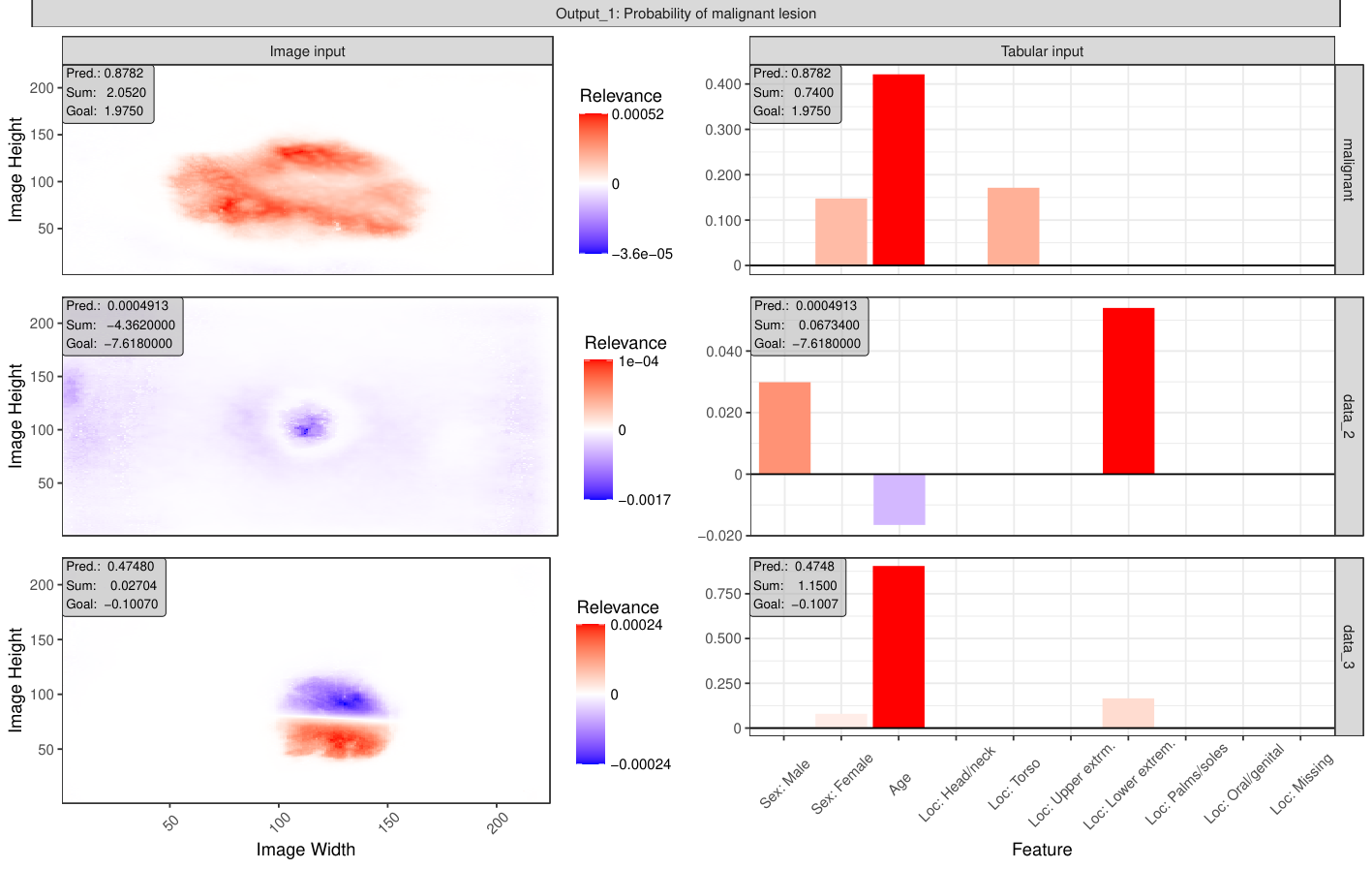
The three instances in Figure 9 describe different explanatory approaches to the trained model’s predictions: The top image in Figure 9(a) of a malignant lesion was recorded on the torso of a -year-old female patient. In the associated interpretation generated by \pkginnsight (top row in Fig. 9(b)), it can be observed that, on the one hand, the model identifies the lesioned skin area. On the other hand, the darker and patchy pigmentation and the ragged borders positively influenced the prediction of for melanoma (shown as in the corresponding infobox in Fig. 9(b)). This observation is also consistent with the official ABCD checklist for melanoma (Friedman et al. 1985), which states that asymmetry, irregular borders, varying color, and large diameters are indicative of a malignant skin lesion. However, the patient’s age also positively affected the prediction, as evident from the tabular patient-level information explanation in Figure 9(b). A complimentary picture results from the middle image in Figure 9(a), showing a benign mole located on the lower extremities of a -year-old man. The model predicted a probability of only for a malignant lesion and explains its decision with the symmetrical shape, uniform color pigmentation, and lack of notched borders. In addition, the age of also has a slightly negative influence on the prediction, whereas the location seems to contribute a large positive effect (middle row in Fig. 9(b)). The last instance exemplifies a situation where the model is uncertain whether it is a malignant or benign skin lesion since its prediction is . The truly malignant skin area originates from the lower extremities of a -year-old woman (bottom image in Fig. 9(a)). Especially the image input explanation in the last row in Figure 9(b) shows the model’s uncertainty because the mole’s upper part looks very regular, arguing for a healthy lesion and consistently highlighted with negative relevance (blue) by the model’s explanation. In contrast, the lower part contains some notches potentially favoring melanoma, which the model also correctly identified. Furthermore, the high age of the -year-old patient has a strong positive relevance to the model’s prediction, demonstrating the strong effect of the feature age. The corresponding infoboxes in Figure 9(b) also show that – while the decomposition goals are not achieved, which, however, is expected in LRP due to the absorption of relevance into the bias vectors – the majority of relevance for the top two patients comes from the image and less from patient-level data. Only in the case of the last patient do the image relevances seem to cancel each other out so that the tabular features have the strongest contribution to the prediction.
5 Validation and runtime
To evaluate the validity and computational performance of \pkginnsight, the results of the presented feature attribution methods on simulated models and data are compared with the results of the \proglangPython implementations \pkgzennit (Anders et al. 2021), \pkginnvestigate (Alber et al. 2019), \pkgcaptum (Kokhlikyan et al. 2020), \pkgdeeplift (Shrikumar et al. 2017a), and \pkgshap (Lundberg and Lee 2017). The packages \pkgdeeplift and \pkginnvestigate are based on the high-level machine learning library \pkgKeras (Chollet et al. 2015) and utilize \pkgTensorFlow (Abadi et al. 2015) as the backend for all calculations. In addition, both packages initially create a replication of the passed model with the interpretation methods pre-implemented in the individual layers, similar to \pkginnsight. In contrast, the packages \pkgzennit and \pkgcaptum use \pkgPyTorch (Paszke et al. 2019) and run without a conversion step since hooks are used to modify the automated backward pass according to the applied method on the fly (see Appendix B for more details). The package \pkgshap can handle both \pkgKeras and \pkgPyTorch models, and also uses hooks to modify automatic gradients. However, this only enables the application of methods that can be considered independent of the preceding and following layers, which complicates, for example, an implementation of DeepLift with the RevealCancel rule. Furthermore, not every package supports all methods. For example, \pkginnvestigate and \pkgzennit are more geared towards standard gradient methods and LRP, whereas \pkgdeeplift is more or less an implementation of the methods from its associated paper and focuses on the DeepLift method. \pkgshap, originating from a methods paper, primarily considers Shapley-value-based methods. On the other hand, \pkgcaptum is a good all-rounder, but still has some gaps in the context of LRP. A summary of the packages’ implemented feature attribution methods is provided in Table 1.
Package \pkg captum \pkg deeplift \pkg innvestigate \pkg shap \pkg zennit \pkg innsight Gradient ✖ SmoothGrad ✖ GradientInput ✖ IntegratedGradient ∗ ✖ ExpectedGradient ✖ ✖ ✖ LRP (simple rule) ✖ ✖ LRP (-rule) ✖ ✖ LRP (--rule) ✖ ✖ † ✖ DeepLift (rescale) ✖ ✖ ✖ DeepLift (reveal-cancel) ✖ ✖ ✖ ✖ DeepSHAP ✖ ✖ ‡ ✖ ∗\pkgdeeplift applies the middle Riemann sum, whereas \pkgcaptum, \pkgzennit and \pkginnsight use right Riemann sum. †\pkginnvestigate uses another definition of the positive and negative part of the bias vector (see. Appendix E). ‡ For max pooling layers, \pkgshap uses the cross maximal value of the and reference value instead their individual maximal value.
5.1 Validity comparison
For the validation, shallow untrained dense and convolutional models with the most commonly used layer types – such as 2D convolution, 2D maximum/average pooling, and dense layers – and normally distributed input data are generated. More specifically, different architectures are considered, using ReLU and hyperbolic tangent to include both constrained and unconstrained activation functions, with and without bias vectors, with varying pooling layers, and a different number of output nodes. From each of these architectures, randomly initialized models are created, resulting in distinct models, and evaluated on normally distributed datasets with input instances each. The experimental details can be found in the Appendix D.1. Moreover, all figures and results are reproducible using the code in the reproduction material or on GitHub (https://github.com/bips-hb/JSS_innsight).
As a measure of quality, the mean absolute difference between the results of \pkginnsight and the corresponding reference implementation over all input variables and output nodes is considered. Consequently, for each combination of method, model, input instance, and output node, a value for this quality measure is derived, leading to box plots for visualizing the differences. In addition to the box plots, an acceptable error range of up to is highlighted in light gray to distinguish numerical tolerated differences caused by calculations of single-precision floating point numbers according to the IEEE 754 standard (IEEE 2019) from abnormal discrepancies. The results are summarized in Figure 10.


For the gradient-based methods Gradient and GradientInput, the method’s results mostly coincide for all packages (see Fig. 10(a)). The only discrepancy is with the IntegratedGradient method for the package \pkgdeeplift, but this is due to the fact that \pkginnsight approximates the integral with the right and \pkgdeeplift with the middle Riemann sum33 3 see https://github.com/kundajelab/deeplift/blob/master/deeplift/util.py#L261. The right Riemann sum is also used in \pkgzennit44 4 see https://github.com/chr5tphr/zennit/blob/0.5.1/src/zennit/attribution.py#L453, whereas various approximation methods can be selected in \pkgcaptum.
A similar picture results for the DeepLift method with the Rescale and RevealCancel rules, but with a few outliers with a maximum error of up to for the Rescale rule (see Fig. 10(b)). However, all outliers with an error exceeding originate from models with the hyperbolic tangent as activation and can thus be explained by numerical inaccuracies due to the saturated activation. In addition, minor discrepancies are probably caused by different treatments of vanishing denominators in the multipliers or numerical uncertainties between the backends \pkgPyTorch/\pkgLibTorch and \pkgTensorFlow in general. With the DeepSHAP method – similar to IntegratedGradient – the results of \pkginnsight largely match those of \pkgcaptum, but they differ from the results of \pkgshap. However, this is mainly due to the max pooling layer (see Fig. 10(b)), which is handled differently in \pkgshap than in \pkginnsight and \pkgcaptum. Since DeepSHAP is a repeated application of DeepLift with different reference values, the numerical inaccuracies from the DeepLift method accumulate and, thus, cause the visible outliers.
For the LRP methods, a few adjustments are needed for the \pkginnvestigate and \pkgcaptum packages since they use only the simple rule for average pooling layers, which is modified in \pkginnsight using composite rules. Apart from that, the results from \pkginnsight compared to \pkgcaptum or \pkgzennit for the simple, -rule and --rule differ negligibly and are far below the maximally tolerated error of (see Fig. 10(c)). For the simple and -rule, \pkginnvestigate is consistent with \pkginnsight except for a few deviations. Again, almost all of the cases with errors exceeding are caused by a saturated hyperbolic tangent activation, lower errors on different stabilizers for the denominators in the relevance messages, and general numerical inaccuracies between their backends. However, significant discrepancies can be observed using the --rule, which only occur in models with a bias vector (see Fig. 10(c) bottom). The reason for this is a different interpretation of the positive or negative part of the bias vector, which is discussed in more detail in the Appendix E.
5.2 Runtime comparison
In addition to comparing whether \pkginnsight’s results are consistent with the reference implementations, a runtime comparison is also conducted concerning the number of output nodes, hidden units or filters, hidden layers, batch size, and, for images, the size of the input images. It must be noted again that the packages based on \pkgKeras and \pkginnsight first convert the passed model, and the \pkgPyTorch-based packages use hooks to overwrite the automated backward pass while executing, making them considerably faster. Therefore, in the results, only the execution time excluding the conversion step – as far as possible – is presented and not the total time. For comparisons of the total time needed to calculate an explanation, see Appendix D.3. However, the \pkginnvestigate package has a special characteristic in this regard since the entire conversion process and the construction of the underlying graph only happens during the analysis of the first batch of input data55 5 See the GitHub issue #50 and #129 for the \pkginnvestigate package.. For this reason, conversion times are almost hardly present in the results. Since this simulation assumes that an interpretation method is being applied for the first time to a model and only to a single batch of input instances, the results of \pkginnvestigate are slightly biased and would be notably quicker if the same model is employed with more input batches.
Analogously to the comparison from Section 5.1, untrained dense and convolutional neural networks, and normally distributed input data are used for the time comparisons. Depending on the type of time comparison, the hyperparameters for the number of output nodes, number of hidden units or filter size, number of hidden layers, batch size, and the size of the input images are varied. The hyperparameters not considered in the respective comparison remain unchanged and take default values, i.e., one output node, hidden units for the tabular model and filters for the image model, two layers in total, a batch size of and an input image size of . In addition, replicates of each architecture are created to compensate for potential numerical fluctuations. For a more detailed simulation description or analysis of the results, including the total time, please refer to Appendix D.2 and D.3, and for a reproduction of the results, see the reproduction material or the code in the GitHub repository at https://github.com/bips-hb/JSS_innsight/.
In general, comparing the runtimes of the different packages reveals that \pkginnsight is faster than \pkginnvestigate and \pkgdeeplift (which are based on \pkgKeras), but slower than \pkgcaptum, \pkgzennit and \pkgshap (which are based on \pkgPyTorch). This overall trend is particularly evident when adding more layers to dense models: \pkginnsight is - times slower than \pkgcaptum and \pkgzennit, but still for the same order of magnitude faster or even faster than \pkginnvestigate and \pkgdeeplift (see Fig. 11(a)). In addition, \pkginnsight is similarly fast as \pkgshap for the methods DeepSHAP and ExpectedGradient. This trend can largely be extended to image inputs as well, with the exception that the evaluation times in \pkginnsight approach those of \pkgPyTorch-based implementations very closely. However, the DeepLift methods, particularly with the Rescale rule and thus even more with DeepSHAP, are considerably slower when applied to images compared to \pkgdeeplift (see Fig.15).
The same trend can also be observed for a varying number of output nodes. In the case of image data, \pkginnsight is similarly fast as the \pkgPyTorch-based packages and mostly considerably faster than \pkginnvestigate and \pkgdeeplift. However, the exception concerning the DeepLift methods applies here as well: DeepLift using the Rescale rule runs almost times slower than in \pkgcaptum. Consequently, DeepSHAP is also considerably slower than the runtime in \pkgshap and \pkgcaptum (see Fig.11(b)). On the other hand, \pkginnsight stands out for all rule-based methods applied to dense models and performs similarly or even faster than the \pkgPyTorch-based packages (see Fig.14). The primary reason for this is that the results for several output nodes can be calculated at once in \pkginnsight. In contrast, all other implementations only allow the calculation for single nodes, and thus, the method’s results are computed by iterative execution.
These tendencies can also be observed in the other simulations’ results when changing the number of hidden units/filters, batch size, or image size (see Fig. 16, 17 and 18 in the Appendix). In the gradient-based methods and LRP, the execution times of \pkginnsight are increasingly approaching the times of the \pkgPyTorch-based implementations. With a larger number of filters in the convolutional models, the runtimes are almost identical. At the same time, it can be seen that the \pkgKeras-based packages run considerably slower than all other packages. An exception to this is with a high number of filters in convolutional models: in these cases, \pkginnvestigate and \pkginnsight applied to standard gradient-based methods and LRP are faster than all other implementations. In addition, the previously observed pattern with the DeepLift methods repeats in the other simulations as well: the execution time of DeepLift with the Rescale rule for image data is noticeably slower than in the reference implementations, which also explains the high execution time of DeepSHAP. Nevertheless, \pkginnsight is considerably faster than \pkgdeeplift in dense models running DeepLift methods, and, in the case of batch size, also faster than \pkgshap.
In summary, \pkginnsight is mostly faster than the \pkgKeras-based packages and becomes more comparable to the \pkgPyTorch packages with increasing number of input instances, hidden units/filters, image size, and number of output nodes. However, the evaluation time of DeepLift with the Rescale rule and DeepSHAP applied to images is a weakness of \pkginnsight and shows the largest discrepancy in the runtime comparison. Even though the packages in this section are compared regarding runtime and some packages’ weaknesses are revealed, all considered implementations provide an explanation within a reasonable time of a few seconds, even for deep neural networks with several large images as inputs.
6 Summary and discussion
In summary, we have presented \pkginnsight, an \proglangR package that provides the most well-known feature attribution methods for interpreting neural network predictions. After a detailed introduction of the implemented feature attribution methods, the internal structure utilizing \pkgtorch’s fast array calculations and conversion function \codeconvert() for initializing an \codeConverter object demonstrated how the deep-learning-model-agnostic approach was implemented to enable the analysis of models from any \proglangR package in an efficient way. This flexibility is complemented by a unified 3-step approach from model to plotted results, including multiple visualization tools based on \pkgggplot2 or \pkgplotly for interactive plots. The step-wise procedure was illustrated using a model on the tabular penguin dataset and a deep neural network on the melanoma dataset consisting of structured patient-level information and images. Furthermore, the results of the simulation study show that \pkginnsight returns nearly identical feature-wise explanations to the reference implementations \pkgcaptum, \pkgzennit, \pkginnvestigate, \pkgdeeplift, and \pkgshap in \proglangPython. Any observed differences are either below the accepted error tolerance of , reflecting negligible numerical inaccuracies, or caused by variations in layer treatments, e.g., max pooling layer in \pkgshap for DeepSHAP or another integral estimation for IntegratedGradient in \pkgdeeplift. In terms of runtime, the package shows that it is generally faster than the \pkgKeras-based packages and slower or comparable fast than \pkgcaptum, \pkgzennit, and \pkgshap. It only suffers with the DeepLift method using the Rescale rule for image data, which is also reflected in the DeepSHAP method that builds on it. Apart from that, the package also has some limitations that could be improved in the future. For example, only converting sequential models (i.e., \codenn_sequential) from the \pkgtorch package is possible because no structured network graph can be extracted from an arbitrary \codenn_module. For all the gradient-based methods, however, this is not strictly necessary, which is why these could be extended for arbitrary \codenn_modules. Nevertheless, passing a model as a list allows the user to do the conversion step on their own in such cases. The package can also be extended methodically and offer permutation-based methods, e.g., Occlusion or RISE (Zeiler and Fergus 2014; Petsiuk et al. 2018). Furthermore, an activation function is assigned to a linear or convolutional layer only if it is defined in the layer itself or immediately after the layer. This behavior is especially relevant for the RevealCancel rule in the DeepLift method, because \pkginnsight handles separated activations with the Rescale rule, which is the case, for example, with the layer sequence of convolution, batch normalization, and activation. Moreover, even if it is possible in the \pkgtorch package, the \pkginnsight package currently only supports computations on CPUs and not on GPUs.
Computational details
A 64-bit Linux platform running Ubuntu 20.04 with an AMD Ryzen Threadrippper 3960X (24 cores, 48 threads) CPU including 256 gigabyte RAM and two NVIDIA Titan RTX GPUs was used for all computations. All comparisons and calculations with the reference implementations were performed in a separate session – created by \pkgcallr (Csárdi and Chang 2022) – using only a single CPU thread per job. An exception was the neural network training on the melanoma dataset using a single GPU, which was also the only code executed by \proglangPython and not from \proglangR 4.3.2 (\proglangR Core Team 2023). Due to the package requirement mismatch, separate environments were created for each of the \pkgKeras-based and the \pkgPyTorch-based packages, i.e.,
- •
\pkg
innvestigate 2.0.2: Using \proglangPython 3.8.15 with \pkgKeras 2.10.0 and \pkgTensorFlow 2.10
- •
\pkg
deeplift 0.6.13: Using \proglangPython 3.6.15 with \pkgKeras 2.2.4 and \pkgTensorFlow 1.15
- •
\pkg
captum 0.6.0, \pkgzennit 0.5.0 and \pkgshap 0.44.0: Using \proglangPython 3.8.12 with \pkgPyTorch 1.13.1 (cpu)
The corresponding environments were loaded in \proglangR, and then the code was executed in \proglangPython using \pkgreticulate 1.34 (Ushey et al. 2023). In addition, the computer was used exclusively for the runtime measurements for the corresponding job and was not distorted by other simultaneous processes.
Acknowledgments
This project was funded by the German Research Foundation (DFG), Emmy Noether Grant 437611051.
References
- Abadi et al. (2015) Abadi M, Agarwal A, Barham P, Brevdo E, Chen Z, Citro C, Corrado GS, Davis A, Dean J, Devin M, Ghemawat S, Goodfellow I, Harp A, Irving G, Isard M, Jia Y, Jozefowicz R, Kaiser L, Kudlur M, Levenberg J, Mané D, Monga R, Moore S, Murray D, Olah C, Schuster M, Shlens J, Steiner B, Sutskever I, Talwar K, Tucker P, Vanhoucke V, Vasudevan V, Viégas F, Vinyals O, Warden P, Wattenberg M, Wicke M, Yu Y, Zheng X (2015). “\pkgTensorFlow: Large-Scale Machine Learning on Heterogeneous Systems.” URL https://www.tensorflow.org/.
- Alber et al. (2019) Alber M, Lapuschkin S, Seegerer P, Hägele M, Schütt KT, Montavon G, Samek W, Müller KR, Dähne S, Kindermans PJ (2019). “\pkgiNNvestigate Neural Networks!” Journal of Machine Learning Research, 20(93), 1–8. URL https://jmlr.org/papers/v20/18-540.html.
- Ancona et al. (2018) Ancona M, Ceolini E, Öztireli C, Gross M (2018). “Towards Better Understanding of Gradient-Based Attribution Methods for Deep Neural Networks.” In Proceedings of the 6th International Conference on Learning Representations. URL https://openreview.net/forum?id=Sy21R9JAW.
- Anders et al. (2019) Anders CJ, Montavon G, Samek W, Müller KR (2019). “Understanding Patch-Based Learning of Video Data by Explaining Predictions.” In Explainable AI: Interpreting, Explaining and Visualizing Deep Learning, Lecture Notes in Computer Science, pp. 297–309. Springer-Verlag. 10.1007/978-3-030-28954-6_16.
- Anders et al. (2021) Anders CJ, Neumann D, Samek W, Müller KR, Lapuschkin S (2021). “Software for Dataset-wide XAI: From Local Explanations to Global Insights with \pkgZennit, CoRelAy, and ViRelAy.” arXiv.org E-Print. 10.48550/arXiv.2106.13200.
- Apley and Zhu (2020) Apley DW, Zhu J (2020). “Visualizing the Effects of Predictor Variables in Black Box Supervised Learning Models.” Journal of the Royal Statistical Society B, 82(4), 1059–1086. 10.1111/rssb.12377.
- Arras et al. (2022) Arras L, Osman A, Samek W (2022). “CLEVR-XAI: A Benchmark Dataset for the Ground Truth Evaluation of Neural Network Explanations.” Information Fusion, 81, 14–40. 10.1016/j.inffus.2021.11.008.
- Auguie (2017) Auguie B (2017). \pkggridExtra: Miscellaneous Functions for "Grid" Graphics. \proglangR package version 2.3, URL https://CRAN.R-project.org/package=gridExtra.
- Bach et al. (2015) Bach S, Binder A, Montavon G, Klauschen F, Müller KR, Samek W (2015). “On Pixel-Wise Explanations for Non-Linear Classifier Decisions by Layer-Wise Relevance Propagation.” Public Library of Science One, 10(7), 1–46. 10.1371/journal.pone.0130140.
- Bengio et al. (2021) Bengio Y, Lecun Y, Hinton G (2021). “Deep Learning for AI.” Communications of the Association for Computing Machinery, 64(7), 58–65. 10.1145/3448250.
- Biecek (2018) Biecek P (2018). “\pkgDALEX: Explainers for Complex Predictive Models in \proglangR.” Journal of Machine Learning Research, 19(84), 1–5. URL http://jmlr.org/papers/v19/18-416.html.
- Chang (2021) Chang W (2021). \pkgR6: Encapsulated Classes with Reference Semantics. https://r6.r-lib.org, https://github.com/r-lib/R6/.
- Chollet et al. (2015) Chollet F, et al. (2015). “\pkgKeras.” https://keras.io.
- Csárdi (2023) Csárdi G (2023). \pkgcli: Helpers for Developing Command Line Interfaces. \proglangR package version 3.6.2, URL https://CRAN.R-project.org/package=cli.
- Csárdi and Chang (2022) Csárdi G, Chang W (2022). \pkgcallr: Call \proglangR from \proglangR. https://callr.r-lib.org, https://github.com/r-lib/callr#readme.
- Erion et al. (2021) Erion G, Janizek JD, Sturmfels P, Lundberg SM, Lee SI (2021). “Improving Performance of Deep Learning Models with Axiomatic Attribution Priors and Expected Gradients.” Nature Machine Intelligence, 3(7), 620–631. 10.1038/s42256-021-00343-w.
- European Union (2016) European Union (2016). “Regulation (EU) 2016/679 of the European Parliament and of the Council of 27 April 2016 on the Protection of Natural Persons with regard to the Processing of Personal Data and on the Free Movement of such Data, and Repealing Directive 95/46/EC (General Data Protection Regulation).” Official Journal L119, 59, 1–88. URL https://eur-lex.europa.eu/eli/reg/2016/679/oj.
- Falbel and Luraschi (2023) Falbel D, Luraschi J (2023). \pkgtorch: Tensors and Neural Networks with ’GPU’ Acceleration. https://torch.mlverse.org/docs, https://github.com/mlverse/torch.
- Fanaee-T (2013) Fanaee-T H (2013). “Bike Sharing Dataset.” UCI Machine Learning Repository. 10.24432/C5W894.
- Fisher et al. (2019) Fisher A, Rudin C, Dominici F (2019). “All Models are Wrong, but Many are Useful: Learning a Variable’s Importance by Studying an Entire Class of Prediction Models Simultaneously.” Journal of Machine Learning Research, 20(177), 1–81. URL https://jmlr.org/papers/v20/18-760.html.
- Friedman (2001) Friedman JH (2001). “Greedy Function Approximation: A Gradient Boosting Machine.” The Annals of Statistics, 29(5), 1189–1232. 10.1214/aos/1013203451.
- Friedman et al. (1985) Friedman RJ, Rigel DS, Kopf AW (1985). “Early Detection of Malignant Melanoma: The Role of Physician Examination and Self-Examination of the Skin.” CA: A Cancer Journal for Clinicians, 35(3), 130–151. 10.3322/canjclin.35.3.130.
- Goldstein et al. (2015) Goldstein A, Kapelner A, Bleich J, Pitkin E (2015). “Peeking Inside the Black Box: Visualizing Statistical Learning With Plots of Individual Conditional Expectation.” Journal of Computational and Graphical Statistics, 24(1), 44–65. 10.1080/10618600.2014.907095.
- Goodman and Flaxman (2017) Goodman B, Flaxman S (2017). “European Union Regulations on Algorithmic Decision-Making and a “Right to Explanation”.” AI Magazine, 38(3), 50–57. 10.1609/aimag.v38i3.2741.
- Greenwell (2023) Greenwell B (2023). \pkgfastshap: Fast Approximate Shapley Values. \proglangR package version 0.1.0, URL https://CRAN.R-project.org/package=fastshap.
- Greenwell et al. (2018) Greenwell BM, Boehmke BC, McCarthy AJ (2018). “A Simple and Effective Model-Based Variable Importance Measure.” arXiv.org E-Print. 10.48550/arXiv.1805.04755.
- Gunning and Aha (2019) Gunning D, Aha D (2019). “DARPA’s Explainable Artificial Intelligence (XAI) Program.” AI Magazine, 40(2), 44–58. 10.1609/aimag.v40i2.2850.
- Günther and Fritsch (2010) Günther F, Fritsch S (2010). “\pkgneuralnet: Training of Neural Networks.” \proglangR Journal, 2(1), 30–38. 10.32614/RJ-2010-006.
- Haug et al. (2022) Haug J, Zürn S, El-Jiz P, Kasneci G (2022). “On Baselines for Local Feature Attributions.” arXiv.org E-Print. 10.48550/arXiv.2101.00905.
- He et al. (2016) He K, Zhang X, Ren S, Sun J (2016). “Deep Residual Learning for Image Recognition.” In Proceedings of the 2016 IEEE Conference on Computer Vision and Pattern Recognition, pp. 770–778. IEEE. 10.1109/CVPR.2016.90.
- Horst et al. (2020) Horst AM, Hill AP, Gorman KB (2020). \pkgpalmerpenguins: Palmer Archipelago (Antarctica) Penguin Data. 10.5281/zenodo.3960218. \proglangR package version 0.1.1.
- Hvitfeldt et al. (2022) Hvitfeldt E, Pedersen TL, Benesty M (2022). \pkglime: Local Interpretable Model-Agnostic Explanations. \proglangR package version 0.5.3, URL https://CRAN.R-project.org/package=lime.
- IEEE (2019) IEEE (2019). “IEEE Standard for Floating-Point Arithmetic.” IEEE Std 754-2019 (Revision of IEEE 754-2008), pp. 1–84. 10.1109/IEEESTD.2019.8766229.
- Kalinowski et al. (2023) Kalinowski T, Falbel D, Allaire J, Chollet F, RStudio, Google, Tang Y, Van Der Bijl W, Studer M, Keydana S (2023). \pkgkeras: \proglangR Interface to \pkgKeras. \proglangR package version 2.13.0, URL https://CRAN.R-project.org/package=keras.
- Kim et al. (2018) Kim B, Wattenberg M, Gilmer J, Cai C, Wexler J, Viegas F, et al. (2018). “Interpretability Beyond Feature Attribution: Quantitative Testing with Concept Activation Vectors (TCAV).” In Proceedings of the 35th International Conference on Machine Learning, volume 80, pp. 2668–2677. PMLR. URL https://proceedings.mlr.press/v80/kim18d.html.
- Kindermans et al. (2019) Kindermans PJ, Hooker S, Adebayo J, Alber M, Schütt KT, Dähne S, Erhan D, Kim B (2019). “The (Un)reliability of Saliency Methods.” Explainable AI: Interpreting, Explaining and Visualizing Deep Learning, pp. 267–280. 10.1007/978-3-030-28954-6_14.
- Kohlbrenner et al. (2020) Kohlbrenner M, Bauer A, Nakajima S, Binder A, Samek W, Lapuschkin S (2020). “Towards Best Practice in Explaining Neural Network Decisions with LRP.” In Proceedings of the 2020 International Joint Conference on Neural Networks, pp. 1–7. IEEE. 10.1109/IJCNN48605.2020.9206975.
- Kokhlikyan et al. (2020) Kokhlikyan N, Miglani V, Martin M, Wang E, Alsallakh B, Reynolds J, Melnikov A, Kliushkina N, Araya C, Yan S, Reblitz-Richardson O (2020). “\pkgCaptum: A Unified and Generic Model Interpretability Library for \pkgPyTorch.” arXiv.org E-Print. 10.48550/arXiv.2009.07896.
- Krizhevsky et al. (2017) Krizhevsky A, Sutskever I, Hinton GE (2017). “ImageNet Classification with Deep Convolutional Neural Networks.” Communications of the Association for Computing Machinery, 60(6), 84–90. 10.1145/3065386.
- Lang (2017) Lang M (2017). “\pkgcheckmate: Fast Argument Checks for Defensive \proglangR Programming.” The \proglangR Journal, 9(1), 437–445. 10.32614/RJ-2017-028.
- Lauritsen et al. (2020) Lauritsen SM, Kristensen M, Olsen MV, Larsen MS, Lauritsen KM, Jørgensen MJ, Lange J, Thiesson B (2020). “Explainable Artificial Intelligence Model to Predict Acute Critical Illness from Electronic Health Records.” Nature Communications, 11(1), 3852. 10.1038/s41467-020-17431-x.
- LeCun et al. (2015) LeCun Y, Bengio Y, Hinton G (2015). “Deep Learning.” Nature, 521(7553), 436–444. 10.1038/nature14539.
- Lundberg and Lee (2017) Lundberg SM, Lee SI (2017). “A Unified Approach to Interpreting Model Predictions.” In Proceedings of the 31st International Conference on Neural Information Processing Systems, pp. 4768–4777. Curran Associates Inc. URL https://dl.acm.org/doi/10.5555/3295222.3295230.
- Molnar et al. (2018) Molnar C, Casalicchio G, Bischl B (2018). “\pkgiml: An \proglangR Package for Interpretable Machine Learning.” Journal of Open Source Software, 3(26), 786. 10.21105/joss.00786.
- Montavon et al. (2019) Montavon G, Binder A, Lapuschkin S, Samek W, Müller KR (2019). “Layer-Wise Relevance Propagation: An Overview.” In Explainable AI: Interpreting, Explaining and Visualizing Deep Learning, Lecture Notes in Computer Science, pp. 193–209. Springer-Verlag. 10.1007/978-3-030-28954-6_10.
- Montavon et al. (2017) Montavon G, Lapuschkin S, Binder A, Samek W, Müller KR (2017). “Explaining Nonlinear Classification Decisions with Deep Taylor Decomposition.” Pattern Recognition, 65, 211–222. 10.1016/j.patcog.2016.11.008.
- Nielsen et al. (2022) Nielsen IE, Dera D, Rasool G, Ramachandran RP, Bouaynaya NC (2022). “Robust Explainability: A Tutorial on Gradient-based Attribution Methods for Deep Neural Networks.” IEEE Signal Processing Magazine, 39(4), 73–84. 10.1109/MSP.2022.3142719.
- Olah et al. (2017) Olah C, Mordvintsev A, Schubert L (2017). “Feature Visualization.” Distill, 2(11), e7.
- Olden et al. (2004) Olden JD, Joy MK, Death RG (2004). “An Accurate Comparison of Methods for Quantifying Variable Importance in Artificial Neural Networks Using Simulated Data.” Ecological Modelling, 178(3), 389–397. 10.1016/j.ecolmodel.2004.03.013.
- O’Sullivan et al. (2019) O’Sullivan S, Nevejans N, Allen C, Blyth A, Leonard S, Pagallo U, Holzinger K, Holzinger A, Sajid MI, Ashrafian H (2019). “Legal, Regulatory, and Ethical Frameworks for Development of Standards in Artificial Intelligence (AI) and Autonomous Robotic Surgery.” The International Journal of Medical Robotics and Computer Assisted Surgery, 15(1), e1968. 10.1002/rcs.1968.
- Paszke et al. (2019) Paszke A, Gross S, Massa F, Lerer A, Bradbury J, Chanan G, Killeen T, Lin Z, Gimelshein N, Antiga L, Desmaison A, Kopf A, Yang E, DeVito Z, Raison M, Tejani A, Chilamkurthy S, Steiner B, Fang L, Bai J, Chintala S (2019). “\pkgPyTorch: An Imperative Style, High-Performance Deep Learning Library.” In Proceedings of the 2019 Conference on Advances in Neural Information Processing Systems, volume 32. Curran Associates. URL https://proceedings.neurips.cc/paper_files/paper/2019/file/bdbca288fee7f92f2bfa9f7012727740-Paper.pdf.
- Petsiuk et al. (2018) Petsiuk V, Das A, Saenko K (2018). “Rise: Randomized Input Sampling for Explanation of Black-Box Models.” arXiv.org E-Print. 10.48550/arXiv.1806.07421.
- \proglangR Core Team (2023) \proglangR Core Team (2023). \proglangR: A Language and Environment for Statistical Computing. \proglangR Foundation for Statistical Computing, Vienna, Austria. URL https://www.R-project.org/.
- Ribeiro et al. (2016) Ribeiro MT, Singh S, Guestrin C (2016). “"Why Should I Trust You?": Explaining the Predictions of Any Classifier.” In Proceedings of the 22nd ACM SIGKDD International Conference on Knowledge Discovery and Data Mining, pp. 1135–1144. Association for Computing Machinery. 10.1145/2939672.2939778.
- Rotemberg et al. (2020) Rotemberg VM, Kurtansky NR, Betz-Stablein B, Caffery LJ, Chousakos E, Codella NCF, Combalia M, Dusza SW, Guitera P, Gutman DA, Halpern AC, Kittler H, Köse K, Langer SG, Liopryis K, Malvehy J, Musthaq S, Nanda J, Reiter O, Shih G, Stratigos AJ, Tschandl P, Weber J, Soyer HP (2020). “A Patient-Centric Dataset of Images and Metadata for Identifying Melanomas Using Clinical Context.” Scientific Data, 8(1). 10.1038/s41597-021-00815-z.
- Schneeberger et al. (2020) Schneeberger D, Stöger K, Holzinger A (2020). “The European Legal Framework for Medical AI.” In Lecture Notes in Computer Science, pp. 209–226. Springer-Verlag, Cham. 10.1007/978-3-030-57321-8_12.
- Shrikumar et al. (2017a) Shrikumar A, Greenside P, Kundaje A (2017a). “Learning Important Features Through Propagating Activation Differences.” In Proceedings of the 34th International Conference on Machine Learning, volume 70, pp. 3145–3153. PMLR. URL https://proceedings.mlr.press/v70/shrikumar17a.html.
- Shrikumar et al. (2017b) Shrikumar A, Greenside P, Shcherbina A, Kundaje A (2017b). “Not Just a Black Box: Learning Important Features Through Propagating Activation Differences.” arXiv.org E-Print. 10.48550/arXiv.1605.01713.
- Sievert (2020) Sievert C (2020). Interactive Web-Based Data Visualization with \proglangR, \pkgplotly, and \pkgshiny. Chapman and Hall/CRC. ISBN 9781138331457. URL https://plotly-r.com.
- Silver et al. (2016) Silver D, Huang A, Maddison CJ, Guez A, Sifre L, van den Driessche G, Schrittwieser J, Antonoglou I, Panneershelvam V, Lanctot M, Dieleman S, Grewe D, Nham J, Kalchbrenner N, Sutskever I, Lillicrap T, Leach M, Kavukcuoglu K, Graepel T, Hassabis D (2016). “Mastering the Game of Go with Deep Neural Networks and Tree Search.” Nature, 529(7587), 484–489. 10.1038/nature16961.
- Simonyan et al. (2014) Simonyan K, Vedaldi A, Zisserman A (2014). “Deep Inside Convolutional Networks: Visualising Image Classification Models and Saliency Maps.” arXiv.org E-Print. 10.48550/arXiv.1312.6034.
- Smilkov et al. (2017) Smilkov D, Thorat N, Kim B, Viégas F, Wattenberg M (2017). “SmoothGrad: Removing Noise by Adding Noise.” arXiv.org E-Print. 10.48550/arXiv.1706.03825.
- Strumbelj and Kononenko (2010) Strumbelj E, Kononenko I (2010). “An Efficient Explanation of Individual Classifications Using Game Theory.” Journal of Machine Learning Research, 11, 1–18.
- Sundararajan et al. (2017) Sundararajan M, Taly A, Yan Q (2017). “Axiomatic Attribution for Deep Networks.” arXiv.org E-Print. 10.48550/arXiv.1703.01365.
- Ushey et al. (2023) Ushey K, Allaire J, Tang Y (2023). \pkgreticulate: Interface to \proglangPython. \proglangR package version 1.34, URL https://CRAN.R-project.org/package=reticulate.
- Wickham (2016) Wickham H (2016). \pkgggplot2: Elegant Graphics for Data Analysis. Springer-Verlag. ISBN 978-3-319-24277-4. URL https://ggplot2.tidyverse.org.
- Wickham and Pedersen (2023) Wickham H, Pedersen TL (2023). \pkggtable: Arrange ’Grobs’ in Tables. https://gtable.r-lib.org, https://github.com/r-lib/gtable.
- Zeiler and Fergus (2014) Zeiler MD, Fergus R (2014). “Visualizing and Understanding Convolutional Networks.” In Computer Vision–ECCV 2014: Proceedings, Part I 13, pp. 818–833. Springer-Verlag. 10.1007/978-3-319-10590-1_53.
- Zuallaert et al. (2018) Zuallaert J, Godin F, Kim M, Soete A, Saeys Y, De Neve W (2018). “SpliceRover: Interpretable Convolutional Neural Networks for Improved Splice Site Prediction.” Bioinformatics, 34(24), 4180–4188. 10.1093/bioinformatics/bty497.
Appendix A Details on LRP and DeepLift
A.1 Details on LRP
The layer-wise relevance propagation (LRP) method was introduced by Bach et al. 2015 and has a similar goal as the GradientInput approach: decomposing the output into variable-wise relevances conforming to Equation 1. The distinguishing aspect is that the prediction is redistributed layer by layer from the output node back to the inputs according to the layer’s weights and intermediate values. The entire procedure is accomplished by rule-based relevance messages defining how to redistribute the upper-layer relevance to the lower layer. More precisely, the relevance message describes the amount of the relevance of node in layer sent to the lower-layer node . The relevance for the lower-layer node is calculated as the sum of all incoming relevance messages, i.e.,
| (6) |
In the following, we briefly overview the most popular variations of relevance messages flowing from a node of index in layer to node in the preceding layer:
- •
The simple rule: The fundamental rule on which all other variations of relevance messages are more or less based is the simple rule (also known as LRP-0). The relevances are redistributed to the lower layers according to the ratio between local and global pre-activation. Let be the inputs of the preceding layer, the weight matrix and the bias vector of layer , and the upper-layer relevance; then is the local and the global pre-activation defining the simple rule as
- •
The -rule: One issue with the simple rule is that it is numerically unstable when the global pre-activation vanishes and causes a division by zero. The -rule (also known as LRP-) tackles those situations by adding a stabilizer that moves the denominator away from zero, i.e.,
This inserted value absorbs some of the relevance and can, therefore, be utilized to achieve sparser and less noisy results for the explanation. As increases, a greater portion of the relevance is intercepted, sustaining only the most salient relevances for this relevance message.
Both variants have in common that they distribute the upper-layer relevance proportionally downward regarding the local and global pre-activations, i.e., and . Even though the -rule avoids division by zero, numerical inconsistencies can occur in both variants for very deep models. Since the pre-activations are not necessarily guaranteed to be positive, the local pre-activations may take on substantial positive or negative values that cancel out in the global pre-activation, leading to magnified values in the preceding layer. As a result, larger relevances in the lower layers potentially accumulate in deep models and increasingly reach the limits of computational representation of floating point numbers. To prevent this blow-up of relevances, the authors introduced the --rule, which treats positive and negative pre-activations separately:
- •
The --rule: The --rule was introduced to avoid numerical instabilities and enable a weighting between positive and negative relevances depending on the user’s focus. This relevance message applies the simple rule to the positive and negative parts of the pre-activations, respectively, and takes the weighted sum of both. The weighting can be regulated by the hyperparameters satisfying . Mathematically formulated, the rule is defined as follows:
Since the bias vector is included in the computation of the global pre-activations in all presented variants, this term absorbs a certain amount of the upper-layer relevance. Consequently, the LRP methods approximate the output prediction rather than providing an accurate representation of the targeted decomposition in Equation 1.
There are even more variants of relevance messages discussed in the literature suitable for various situations or layer types: For example, the deep Taylor decomposition (also called -rule) in ReLU models – also achieved with the --rule with – allows filtering out only positive relevances (Montavon et al. 2017), or the -rule favoring positive over negative relevances (Montavon et al. 2019). Moreover, some rules are specifically designed for the input layer (Montavon et al. 2017). Due to the rule independence of how the lower-layer relevances are computed from the relevance messages in Equation 6, the rules can also be set individually for each layer, called composite-rule (Montavon et al. 2019; Kohlbrenner et al. 2020).
A.2 Details on DeepLift
The deep learning important features (DeepLift) method introduced by Shrikumar et al. 2017a behaves similarly to LRP in a layer-by-layer backpropagation fashion from a selected output node back to the input variables considering the simple rule. However, it incorporates a reference value to compare the relevances with each other. Hence, the relevances of DeepLift represent the relative effect of the outputs of the instance to be explained and the output of the reference value . By taking the difference, the bias term is eliminated in the relevance messages, preventing the relevance absorption and leading to an exact variable-wise decomposition of the difference-from-reference output , i.e.,
In contrast to the LRP method, DeepLift defines a multiplier layer by layer, starting from the output layer and propagating to the input layer instead of directly determining the relevances in each intermediate stage. Based on these multipliers, the contribution of an arbitrary variable to the difference-from-reference output can be obtained by multiplying it by the corresponding difference-from-reference input. For an arbitrary layer with the layer’s input , reference input and multiplier , this means:
| (7) |
The multipliers fulfill a chain rule allowing the computation of the multiplier for the preceding layer given the already calculated one , i.e.,
| (8) |
In other words, the chain rule justifies defining the multipliers for each layer or part of a layer separately before combining them with the upper-layer multipliers. The authors distinguish between the linear and nonlinear components of a layer and provide definitions of the multipliers for each of them:
- •
Linear rule: For the linear components of a layer, such as matrix multiplication in dense or convolution layers, the weights of the corresponding layer are used as the multipliers, i.e., .
- •
Rescale rule: This rule can be used for all nonlinear parts of a layer that can be reduced to a one-dimensional function , e.g., all activations such as ReLU, tanh, or sigmoid. In this case, the ratio between the difference-from-reference activation and the pre-activation gives the multiplier, i.e., . To avoid numerical instability caused by a vanishing denominator, the gradient of at is used instead of the multiplier when is close to its reference value .
- •
RevealCancel rule: This rule is designed for non-linearities to propagate meaningful relevances for saturated activations and discontinuous gradients through the layers’ activation part, even when activations like ReLU eliminate the values. Similar to the normal pre-activations in the --rule for LRP, the positive and negative difference-from-reference pre-activations are considered separately, ensuring the propagation of expressive contribution scores. Descriptively, the RevealCancel rule can be explained in a way that the multiplier for the positive part is the ratio between the average effect of after activating, before and after the negative part has been added, and the positive difference-from-reference pre-activation . In the same way, the negative multiplier is given by the ratio of the average impact of after activating, before and after the positive part has been added, to . Mathematically, the rule is defined as
These rules, along with the chain rule (Equations 7-8), enable the successive computation of the input variables’ contributions to the difference-from-reference output in a single backward pass.
Appendix B Remarks on accepted models and layers
As described in Section 3.1, conversion functions are only provided by default for the packages \pkgtorch, \pkgkeras, and \pkgneuralnet to transfer a neural network into a list structure, which is explained in more detail in the next paragraph. However, any model in this list format can be directly passed to the \codeConverter. When initializing the \codeConverter object, a \pkgtorch-based copy of the model is then generated from this list. This is one of the most crucial differences compared to packages like \pkgcaptum, \pkgzennit, and \pkgshap, as these packages override the automatic differentiation graph in the backward pass of the method through so-called backward hooks66 6 See, e.g., \coderegister_full_backward_hook() in \pkgPyTorch (https://pytorch.org/docs/stable/generated/torch.nn.Module.html#torch.nn.Module.register_full_backward_hook) or \codetf.RegisterGradient in \pkgTensorFlow/\pkgKeras (https://www.tensorflow.org/api_docs/python/tf/RegisterGradient).. Consequently, there is no need to analyze and copy the computational graph of the neural network; instead, adjusting the gradient computation of the relevant layers in the backward pass is sufficient. This feature is not available in version 0.12.0 of \pkgtorch in \proglangR, which is why we opted for copying the layers as in the packages \pkginnvestigate and \pkgdeeplift and extended it to a deep-learning-model-agnostic approach. However, this advantage comes with the requirement that all calculations in the network need to be registered and transferred to \pkgtorch. For example, the gradient function does not need to be overridden and registered for a flatten layer in \pkgcaptum, \pkgzennit and \pkgshap – as it only rearranges the values – aligning with the existing automatic differentiation function. In \pkginnsight, the entire model is copied, so an equivalent in \pkgtorch must be created for this layer as well. In general, every model from the \pkgneuralnet and \pkgkeras packages can be converted. In the case of \pkgkeras, this includes both sequential models created with \codekeras_model_sequential() and non-sequential models created with \codekeras_model(), as long as they only include the accepted layers listed in Table 2. Since it is not possible to reconstruct a computational graph for \pkgtorch models, only \codenn_sequential() models are accepted, and only the layers listed in Table 2 are recognized.
Package \pkgkeras \pkgtorch as \codelist (\codetype =) Dense \codelayer_dense() \codenn_linear() \code"Dense" Convolution \codelayer_conv_1d() \codenn_conv1d() \code"Conv1D" \codelayer_conv_2d() \codenn_conv2d() \code"Conv2D" Pooling \codelayer_max_pooling_1d() \codenn_max_pool1d() \code"MaxPooling1D" \codelayer_max_pooling_2d() \codenn_max_pool2d() \code"MaxPooling2D" \codelayer_average_pooling_1d() \codenn_avg_pool1d() \code"AveragePooling1D" \codelayer_average_pooling_2d() \codenn_avg_pool2d() \code"AveragePooling2D" \codelayer_max_pooling_1d() \code"GlobalPooling" \codelayer_max_pooling_2d() \codelayer_average_pooling_1d() \codelayer_average_pooling_2d() Batch \codelayer_batch_normalization() \codenn_batch_norm1d() \code"BatchNorm" Normalization \codenn_batch_norm2d() Activation \codelayer_activation_relu() \codenn_relu() \code"Activation" \codelayer_activation_leaky_relu() \codenn_leaky_relu() with \code"relu", \code"softplus", \codelayer_activation_softmax() \codenn_softplus() \code"sigmoid", \code"softmax", \codelayer_activation() with \codenn_sigmoid() \code"tanh", \code"linear" \code"relu", \code"softplus", \codenn_softmax() \code"sigmoid", \code"softmax", \code"tanh" \codenn_tanh() Other \codelayer_input() \codenn_flatten() \code"Flatten" \codelayer_flatten() \codenn_dropout() \code"Add" \codelayer_add() \code"Concatenate" \codelayer_concatenate() \code"Padding" \codelayer_zero_padding_1d() \codelayer_zero_padding_2d() \codelayer_dropout()
Internally, a model is being transferred from the packages \pkgkeras, \pkgtorch, and \pkgneuralnet into a list, from which a \pkgtorch-based model is subsequently created. This list requires the entries \code"input_dim" representing the input dimension excluding the batch dimension, \code"layers" for the model’s layers (again a list), and \code"input_nodes"/\code"output_nodes" for the indices of the model’s input and output layers from \code"layers". Additionally, input and output labels can be specified using the entries \code"input_names" and \code"output_names". The input and output names are identical to the fields in the converter object, but when passing a model, they are optional and will be automatically filled otherwise. They always represent a list for each input or output layer, and then contain a list of names for each dimension. For example, \codelist(list("a", "b", "c"), list("1", "2", "3")) is valid as input names for a model with one input layer that expects a two-dimensional input of shape . The entry \code"layers" again forms a list of individual layers of the neural network. For each layer, the \code"type" entry specifies the layer type, and, depending on the type, other relevant components of the layer. For example, a dense layer (\codetype = "Dense") has the entries \code"weight" for the weight matrix and \code"bias" for the bias vector. In addition to these layer-specific entries, each layer has entries \code"input_layers" and \code"output_layers", indicating the indices in \code"layers" of the incoming and outgoing layers. All available layer types are listed in Table 2. For a more detailed description of the entries and the requirements for the other layer types, please refer to the vignette "In-depth explanation" (see \codevignette("detailed_overview", package = "innsight") or the online documentation at https://bips-hb.github.io/innsight/articles/detailed_overview.html). For the model trained on the bike sharing dataset in Section 3, the argument \codesave_model_as_list in the \codeconvert() function can be used to exemplify the list structure for a dense model:
R> conv <- convert(model, + output_names = c("Number of rented bikes/10,000"), + save_model_as_list = TRUE) R> str(conv
Appendix C Advanced visualization
In Sections 3.3 the basic \codeplot() and \codeplot_global() functions have already been explained. As mentioned there, these functions create either an object of the \codeS4 class \codeinnsight_ggplot2 (if \codeas_plotly = FALSE) or one of the \codeS4 class \codeinnsight_plotly (if \codeas_plotly = TRUE). These functions are intended to generalize the usual \pkgggplot2, or \pkgplotly objects since, with these packages, the limits of clear visualization possibilities for models with multiple input layers are quickly reached. For example, two charts with different scales for each output node or class need to be generated in a model with images and tabular data as inputs. In this case, a \pkgggplot2-based or \pkgplotly-based plot is generated for each single input instance and output node and then combined into one large visualization using \codearrangeGrob() from \pkggridExtra (Auguie 2017) or \codesubplot() from \pkgplotly, respectively. In contrast, the \codeS4 class \codeinnsight_ggplot2 behaves as a wrapper for the \pkgggplot2 object for ordinary models with only one input or output layer. Nevertheless, instances of the \codeinnsight_ggplot2 class can be treated and modified as regular \pkgggplot2 objects providing a \pkgggplot2-typical usage by adding, for example, themes, scales, or geometric objects; hence the intermediate step via this class is generally not noticeable to the user. For example, the following code is valid: {Code} plot(method) + ggplot2::theme_bw() + ggplot2::xlab("My new x label") + ggplot2::scale_y_continuous(trans = "pseudo_log") + ggplot2::geom_text(ggplot2::aes(label = signif(value)) Conveniently, all \pkgggplot2 objects are based on the same \codedata.frame, which is also obtained via the \codeget_result() method (see Sec. 3.3.1), i.e., the corresponding column names can be used as variables in the \pkgggplot2 objects, as can be seen in the last line of the code chunk above. For objects of the \codeinnsight_plotly class, the entire plot is always created using the \codeplotly::subplot() function. However, this has the consequence that individually assigned modifications are partially overwritten by the grouping, which is why the usual \pkgplotly-typical adaptations can only be performed after the \codeinnsight_plotly object has been printed and returned by the generic \codeprint() function for this class, i.e., {Code} print(plot(method, as_plotly = TRUE)) plotly::hide_colorbar() plotly::layout(xaxis = list(title = "My new x label")) In addition, generic functions for both \codeS4 classes are implemented, which provide a deeper and more detailed examination of an already created plot through indexing or indexed modification. Section 4.2 demonstrates the application and illustration of some of these generic methods using visualized explanations of a model that takes tabular and image data as inputs. However, for a more detailed description and usage of these classes, please refer to the vignette "In-depth explanation" (see \codevignette("detailed_overview", package = "innsight") or the online documentation at https://bips-hb.github.io/innsight/articles/detailed_overview.html).
Appendix D Simulation details
D.1 Validity comparison
"-n" indicates the number of units for dense and the number of filters for convolutional layers.
In order to verify the correctness of the \pkginnsight package, a comparative simulation is performed with the reference implementations \pkgzennit, \pkgcaptum, \pkginnvestigate, \pkgdeeplift and \pkgshap using convolutional and dense neural networks, for which the basic structure is shown in Figure 12. The dense architecture starts with an input of input variables, then has units in the middle hidden layer and either one or five output units. In addition, either ReLU or hyperbolic tangent is used to consider both unbounded and bounded activation functions. The convolutional architecture starts with inputs of shape and a convolutional layer with five filters and a kernel size of , followed by activation with ReLU or hyperbolic tangent. Models are created with and without a pooling layer, which comes at this point. Average or maximum pooling layers with a kernel size of are used. Nevertheless, if no pooling layer is considered, strides of are used in the preceding convolutional layer to get a similar number of units after flattening. A dense layer with one or five output nodes follows the flattening. Based on these models and normally distributed dataset with input instances, the following methods are compared:
- •
Gradient-based: Gradient, GradientInput, IntegatedGradient with \coden = 20 and with zeros and normally distributed reference values.
- •
LRP: simple rule, -rule with , --rule with and .
- •
DeepLift: Rescale and RevealCancel rule with zeros and normally distributed reference values each.
- •
DeepSHAP with baseline values.
In this comparison, the methods SmoothGrad and ExpectedGradient are excluded because they are based on sampling, and consequently, they would only yield the same results with the exact same seed and calculation order. Basically, both methods, however, rely on the gradient calculation of Gradient or IntegratedGradient. Therefore, an agreement with these methods can also imply the validity of SmoothGrad and ExpectedGradient.
D.2 Runtime comparison
Besides the consistency of the methods’ results, a runtime comparison of basic dense and convolutional models between \pkginnsight and the reference implementations \pkgzennit, \pkgcaptum, \pkginnvestigate and \pkgdeeplift is also performed regarding several aspects: The number of output nodes (C), hidden units or filters (U), depth of the model (L), batch size (B), and for images the height/width (W) are varied resulting in the different architectures described in more detail in Figure 13. In the image model, for the 2D convolutional layer, which is repeated times, a kernel size of with default strides of and padding is applied so that the output shape corresponds to the input shape. But for the subsequent convolutional layer, a valid padding with strides of is used, producing an equal number of flattened values regardless of the height and width of the input image. Overall, the time comparison is performed for the following methods, and the average time of replications is calculated:
- •
Gradient-based: Gradient, GradientInput, IntegratedGradient with \coden = 10 and a normally distributed reference value and ExpectedGradient with normally distributed reference values and samples.
- •
LRP: simple rule, -rule with , --rule with .
- •
DeepLift: Rescale and RevealCancel rule with a normally distributed reference value.
- •
DeepSHAP with normally distributed reference values.
In addition to the total time required by a method of one of the considered packages for generating an explanation, the pure execution time is also measured separately. How exactly the time measurement of each method of the packages is accomplished can be found in the reproduction material or in the GitHub repository at https://github.com/bips-hb/JSS_innsight.
D.2.1 Number of output nodes (C)
In the time analysis regarding the number of output nodes, dense and image models of each of the architecture shown in Figure 13 are created for . The default values are set for the other hyperparameters, i.e., , for the tabular models, for image models, , and . Since \pkginnsight is explicitly designed to analyze multiple output nodes or output classes simultaneously, it is only possible to generate the results in one run with \pkginnsight. All other implementations are forced to perform a for-loop over the output nodes.
D.2.2 Number of layers (L)
In the time analysis regarding the number of hidden layers, dense and image models of each of the architecture shown in Figure 13 are created for . The default values are set for the other hyperparameters, i.e., , , for the tabular models and for image models, and .
D.2.3 Number of hidden units/filters (U)
In the time analysis regarding the number of hidden units for dense models and number of filters for image models, models each of the architecture shown in Figure 13 are created for for the tabular and for the image model. The default values are set for the other hyperparameters, i.e., , , , and .
D.2.4 Batch size (B)
In the time analysis regarding the number of input instances, dense and image models of each of the architecture shown in Figure 13 are created for for tabular and for image models. The default values are set for the other hyperparameters, i.e., , , for the tabular models and for image models, and .
D.2.5 Height and width of the image inputs (W)
In the time analysis regarding the height/width of the image inputs, image models for each of the architecture shown in Figure 13 are created for . The default values are set for the other hyperparameters, i.e., , for the tabular models and for image models, and .
D.3 Additional figures
D.3.1 Number of output nodes (C)
D.3.2 Number of layers (L)
D.3.3 Number of hidden units/filters (U)

D.3.4 Batch size (B)
D.3.5 Height and width of the image inputs (W)
Appendix E LRP with bias for \pkginnvestigate
As already observed in Section 5, the results of \pkginnsight and \pkginnvestigate differ significantly in the LRP method with the --rule for models with a bias vector. In the following, this problem is analyzed using a very simple neural network with only one dense layer consisting of one input variable and one output node. This layer has a weight of , a bias vector of , and is applied to the input . Mathematically, this results in the following input relevance for :
This yields, for example, in a relevance of for the --rule with and for , which are exactly the values that \pkginnsight outputs. The package \pkginnvestigate, on the other hand, outputs relevance and , which is probably because the bias vector is included in the calculation of the positive part despite the negative sign. This short comparison can be reproduced with the reproduction material or in our GitHub repository (https://github.com/bips-hb/JSS_innsight) and is based on version 2.0.2 of \pkginnvestigate.