Understanding and Mitigating Extrapolation Failures in Physics-Informed Neural Networks
Abstract
Physics-informed Neural Networks (PINNs) have recently gained popularity due to their effective approximation of partial differential equations (PDEs) using deep neural networks (DNNs). However, their out of domain behavior is not well understood, with previous work speculating that the presence of high frequency components in the solution function might be to blame for poor extrapolation performance. In this paper, we study the extrapolation behavior of PINNs on a representative set of PDEs of different types, including high-dimensional PDEs. We find that failure to extrapolate is not caused by high frequencies in the solution function, but rather by shifts in the support of the Fourier spectrum over time. We term these spectral shifts and quantify them by introducing a Weighted Wasserstein-Fourier distance (WWF). We show that the WWF can be used to predict PINN extrapolation performance, and that in the absence of significant spectral shifts, PINN predictions stay close to the true solution even in extrapolation. Finally, we propose a transfer learning-based strategy to mitigate the effects of larger spectral shifts, which decreases extrapolation errors by up to .
1 Introduction
Understanding the dynamics of complex physical processes is crucial in many applications in science and engineering. Oftentimes, these dynamics are modeled as partial differential equations (PDEs) that depend on time. In the PDE setting, we want to find a solution function that satisfies a given governing equation of the form
| (1) |
where denotes the partial derivative of with respect to time, is a - generally nonlinear - differential operator, , with is a spatial domain, and is the final time for which we’re interested in the solution. Moreover, we impose an initial condition , on , as well as a set of boundary conditions. Together, these conditions specify the behaviors of the solution on the boundaries of the spatio-temporal domain.
Following the recent progress in deep learning, physics-informed neural networks (PINN) as introduced in Raissi et al. 2019 have garnered attention because of their simple, but effective way of approximating time-dependent PDEs with deep neural networks. PINNs preserve important physical properties described by the governing equations by parameterizing the solution and the governing equation simultaneously with a set of shared network parameters. After the success of the seminal paper Raissi et al. 2019, many sequels have applied PINNs to solve various PDE applications, e.g. Anitescu et al. 2019; Yang et al. 2021; Zhang et al. 2018; Doan et al. 2019. Physics-informed loss terms have also proven useful in machine learning more generally Davini et al.; Cai et al. 2021.
Related work. Most previous studies using the standard PINNs introduced in Raissi et al. 2019 have demonstrated the performances of their methods in interpolation only, i.e. on a set of testing points sampled within the same temporal range that the network was trained on. We refer to points sampled beyond the final time of the training domain as extrapolation. In principle, standard PINNs are expected to be able to learn the dynamics in Eq. (1) and, consequently, to approximate accurately in extrapolation. However, previous work in Kim et al. 2020 and Bonfanti et al. 2023 has shown that this is not the case: PINNs can deviate significantly from the true solution once they are evaluated in an extrapolation setting, calling into question their capability as a tool for learning the dynamics of physical processes.
From a foundational standpoint, studying extrapolation can therefore give us insights into the limitations of PINNs more generally. From a practical standpoint, constantly retraining PINNs from scratch when faced with a point that is outside their initial training domain is undesirable (Bonfanti et al. 2023; Zhu et al. 2022), so anticipating whether their predictions remain accurate is crucial. Several recent papers have recognized the importance of the extrapolation problem in PINNs (Kapoor et al. 2023; Bonfanti et al. 2023; Cuomo et al. 2022; Kim et al. 2020), and at least two have proposed methods to address it (Kim et al. 2020; Kapoor et al. 2023). However, even a basic characterization of extrapolation behavior for PINNs trained to solve time-dependent PDEs is still absent from the literature. Previous works consider standard PINNs incapable of extrapolating beyond the training domain and suspect implicit biases in deep neural networks to lead to the learned solution becoming smooth or flat in extrapolation, thus implying that the presence of high frequencies in the solution function might lead to extrapolation failures (Bonfanti et al. 2023). Finally, there are to the best of our knowledge no theoretical works on the extrapolation capabilities of PINNs. Previous works have focused on PINN generalization in interpolation only (Mishra and Molinaro 2022).
Contributions. In this paper, our contributions are therefore as follows. (i) We show that PINNs are capable of almost perfect extrapolation behavior for certain PDEs. (ii) We characterize these PDEs by analyzing the Fourier spectra of their solution functions and argue that standard PINNs generally fail to anticipate shifts in the support of the Fourier spectrum over time. We quantify these spectral shifts using the Wasserstein-Fourier distance. (iii) We clarify that unlike with training failures in interpolation, the presence of high frequencies alone is not to blame for the poor extrapolation behavior of PINNs on some PDEs. (iv) We show that these insights generalize to high-dimensional PDEs, and (v) we demonstrate the transfer learning on a set of similar PDEs can reduce extrapolation errors significantly when spectral shifts are present.
The structure of the paper is as follows: in section 2, we formally introduce PINNs and define what we mean by interpolation and extrapolation. Section 3 characterizes the PDEs for which good extrapolation accuracy is possible using the Fourier spectra of their solution functions and introduce the Weighted Wasserstein-Fourier distance. In section 4, we investigate the viability of transfer learning approaches in improving extrapolation. Section 5 discusses our results and concludes.
2 Background and definitions
Physics-Informed Neural Networks. As mentioned in the previous section, PINNs parameterize both the solution and the governing equation . Denote the neural network approximating the solution by and let be the network’s weights. Then the governing equation is approximated by a neural network . The partial derivatives here can be obtained via automatic differentiation. We note that shares its network weights with . The name “physics-informed” neural network comes from the fact that the physical laws we’re interested in are enforced by applying an extra, problem-specific, nonlinear activation, which is defined by the PDE in Eq. (1) (i.e., .
We learn the shared network weights using a loss function consisting of two terms, which are associated with approximation errors in and , respectively. Raissi et al. 2019 considers a loss of the form , where are coefficients and and are defined as follows:
| (2) |
enforces the initial and boundary conditions using a set of training data . The first element of the tuple is the input to the neural network and the second element is the ground truth that the
output of attempts to match. We can collect this data from the specified initial and boundary conditions since we know them a priori. Meanwhile, minimizes the discrepancy between the governing equation and the neural network’s approximation . We evaluate the network at collocation points . Note that here, the ground truth consists of all zeros. We also refer to as the mean absolute residual (MAR): its value denotes how far the network is away from satisfying the governing equation. Note that using this loss, i) no costly evaluations of the solutions at collocation points are required to gather training data, ii) initial and boundary conditions are enforced using a training dataset that can easily be generated, and iii) the physical law encoded in the governing equation in Eq. (1) is enforced by minimizing . In the original paper by Raissi et al. 2019, both loss terms have equal weight, i.e. , and the combined loss term is minimized.
Interpolation and extrapolation. For the rest of this paper, we refer to points as interpolation points if , and as extrapolation points if for . We are primarily interested in the error of the learned solution, i.e. in , and in the relative error, which is the error divided by the norm of the function value at that point, i.e. . When we sample evaluation points from the extrapolation domain, we refer to the (relative) error as the (relative) extrapolation error. Similarly, we are interested in the (mean) absolute residual as defined above, i.e. in . For points sampled from the extrapolation domain, we refer to this as the extrapolation residual.
In this paper, we are interested in the extrapolation performance of PINNs, by which we broadly mean the following questions: how quickly does the performance of a PINN deteriorate as we move away from the interpolation domain? What aspects of the model or underlying PDE affect this? When we speak of ”near perfect” extrapolation, we therefore always mean the accuracy of the model on a bounded extrapolation domain, usually neighboring the interpolation domain. This is in line with Kim et al. 2020 and distinct from the question whether MLPs more generally can extrapolate to arbitrary domains Haley and Soloway 1992; Cardell et al. 1994; Ziyin et al. 2020.
PDEs considered. We investigate the extrapolation capabilities of PINNs on a representative set of 7 PDEs, all of which are widely used as examples in the PINN literature Basir 2022; Raissi et al. 2019; Penwarden et al. 2023; Jagtap and Karniadakis 2021. These include the Allen-Cahn equation, the viscous Burger’s equation, a heat equation, a diffusion equation, a diffusion-reaction equation, the Beltrami flow, and the non-linear Schrodinger equation. Details on all PDEs considered can be found in Appendix A.1.
3 Understanding extrapolation failures via spectral shifts
3.1 Effects of model size, activation functions, & number of training samples
Before we begin our investigation of what determines extrapolation performance in PINNs, we identify several aspects of a model that do not have an effect. This will make our analysis in the second half of this section easier. To this end, we analyze the extrapolation errors and residuals which standard PINNs display for the Allen-Cahn equation, the viscous Burgers equation, a diffusion equation, and a diffusion-reaction equation.

PINN extrapolation performance depends on the underlying PDE. For each of the four PDEs introduced above, we train a -layer MLP with neurons per layer and activation on the interpolation domains specified for epochs using the adam optimizer. As seen in Figure 1 observe that the relative errors for the Burgers’ equation and for the Allen-Cahn equation
become significantly larger than for the diffusion and diffusion-reaction equations when we move from to . The solution learned for the diffusion-reaction
equation disagrees only minimally with the true solution, even at , which shows that for this particular PDE, PINNs can extrapolate almost perfectly well. More detailed results can be found in Appendix A.2.
Extrapolation performance is generally independent of model parameters. While we observe drastically different extrapolation behaviors depending on the underlying PDE as mentioned above, the extrapolation for a given PDE seems to be more or less independent of model parameters, such as number of layers or neurons per layer, activation function, number of samples, or training time. Once the chosen parameters allow the model to achieve a low error in the interpolation domain - is a value commonly used for this in the literature Raissi et al. 2019; Chen et al. 2023; Wang et al. 2022; Han and Lee 2021 - adding more layers, neurons, or samples, or alternatively training longer does not seem to have an effect on the extrapolation error and MAR.
These results allow us to focus our further analyses on a single architecture. Unless otherwise stated, we use an MLP with layers with neurons each and activation, initialized with the commonly used Xavier normal initialization, and trained for epochs using Adam.
3.2 Extrapolation in the presence of high frequencies
Recent literature has found that neural networks tend to be biased towards low-complexity solutions due to implicit regularization inherent in their gradient descent learning processes Neyshabur et al. 2014; Neyshabur 2017. In particular, deep neural networks have been found to possess an inductive bias towards learning lower frequency functions, a phenomenon termed the spectral bias of neural networks Rahaman et al. 2019; Cao et al. 2019, which for example Bonfanti et al. 2023 suspect to be related to extrapolation failures in PINNs. They find evidence for this when considering time-independent PDEs.

Following this hypothesis, we would expect most of the extrapolation error to come from the higher frequencies: the predicted function might become smooth or flat in extrapolation, similar to what has been observed with training failures in interpolation Basir 2022. We plot both the reference solution and the predicted solution in the Fourier domain for all four of our PDEs, as well as the absolute difference between the two Fourier spectra of the reference and predicted solution. Plots for the Burgers’ equation are provided in Figure 2 while plots for the other PDEs are provided in Appendix A.3.
High frequencies only account for a small fraction of extrapolation errors. In all cases, the majority of the error in the Fourier domain is concentrated in the lower-frequency regions. While this is partially due to the fact that the low frequency components of the solutions have larger magnitude, it suggests that in extrapolation, PINNs fail even to learn the low frequency parts of the solution. Thus, the presence of high frequencies alone fails to explain the extrapolation failure of PINNs. We provide some additional evidence for this by studying the extrapolation behavior of Multi-scale Fourier feature networks Wang et al. 2020 in Appendix A.6. Even though these architectures were designed specifically to make learning higher frequencies easier, we find their extrapolation error to be at least as large or larger than that of standard PINNs.
PINNs can extrapolate well in the presence of high frequencies. To isolate the effect that the presence of high frequencies alone has on extrapolation performance, we consider the following variation of the Diffusion-Reaction for and .
| (3) | ||||
| (4) |
The reference solution is given by . As with our other experiments, we use as the temporal training domain and consider as the extrapolation area. here is a hyperparameter that controls the size of the spectrum of the solution. Note that for a fixed , the support of the Fourier spectrum of the reference solution never changes over time, with only the amplitudes of each component scaled down by an identical constant factor.

For various values of , we find that our trained PINNs are able to extrapolate well as can be seen in Figure 3 (a). For the sake of completeness, we also investigate the effect of the speed of decay of the amplitudes in the Fourier spectra. We train a PINN on the following variation of the Diffusion-Reaction equation.
| (5) |
for and with the initial condition and the Dirichlet boundary condition . The reference solution is
| (6) |
with the same interpolation and extrapolation areas as before. Figure 3 (b) shows the relative interpolation and extrapolation errors against increasing values of . We find that an increase in the speed of the exponential decay seems to increase the extrapolation error more than an increase in the size of the spectrum.
3.3 Spectral shifts
While the solutions to the Allen-Cahn equation and to the Burger’s equation do not exhibit exponentially fast changes in their amplitudes, they have Fourier spectra whose support shifts over time, unlike the diffusion and diffusion-reaction equations. We argue that PINNs struggle to extrapolate well when these spectral shifts in the true solution’s Fourier spectrum are large.
Weighted Wasserstein-Fourier distance. To quantify the temporal shifts in the support of the Fourier spectrum, we introduce the Weighted Wasserstein-Fourier Distance (WWF) between the normalized Fourier spectra of the PDE solution in two disjoint time domains. The Weighted Wasserstein-Fourier Distance is based on the Wasserstein-Fourier distance, which compares the Fourier spectra of the solution function at two different points in time. Consider two discrete CDFs supported on the domain . The Wasserstein distance between and is defined as . Given two discrete Fourier spectra , the Wasserstein-Fourier distance Cazelles et al. 2020 can be computed as . We now define the Weighted Wasserstein-Fourier Distance given a function as
where and are the interpolation and extrapolation domains, respectively. We present plots of the pairwise Wasserstein-Fourier distances for each in Appendix A.4. The Wasserstein-Fourier distance of the true solution is zero everywhere for both the diffusion and diffusion-reaction equations, leading to a Weighted Wasserstein-Fourier Distance of zero, which reflects the constant support of the spectra. In contrast, the pairwise distance matrices for the Burgers’ and Allen-Cahn equations exhibit a block-like structure, with times in disjoint blocks exhibiting pronouncedly different distributions in the amplitudes of their respective Fourier spectra. These shifts are not captured by the learned solution, leading to large errors.

The Weighted Wasserstein-Fourier distance allows us to capture the effects that other properties of the underlying PDE have on extrapolation performance. To illustrate this, we train PINNs for different Burgers’ equations, each with a different viscosity parameter – equally spaced from 0.001 to 0.1, and for 50 variants of the Allen-Cahn equation with varying values of , equally spaced from 0.0001 to 0.1. We find that different PDE coefficients lead to large differences in extrapolation performance and that this relationship is moderated quite heavily through shifts in the underlying Fourier spectra. Figure 4 plots the WWF distance between the spectra against the relative error in extrapolation. PDE coefficients that induce larger shifts in the spectra correspond to overall worse extrapolation performance.
3.4 Higher-dimensional and more complex PDEs
Our findings so far demonstrate that the extrapolation performance of PINNs depends heavily on the presence of spectral shifts in the underlying PDE. We conclude this section by showing that this remains true for higher-dimensional and more complex PDEs. To this end, we train PINNs on the Beltrami Flow and the non-linear Schrodinger equation.
The reference solution to the non-linear Schrodinger equation exhibits significant shifts in the spectra, with a WWF Distance distance between the interpolation and extrapolation domains of and in the real and imaginary domain respectively. Based on our results for lower-dimensional PDEs, we expect extrapolation performance to be poor. Our experimental results agree: while the PINN achieves a small interpolation error (), it exhibits poor extrapolation behavior, achieving max relative errors of 0.94, and 4.27 (in the real and imaginary domain respectively).
On the other hand, the Beltrami flow does not exhibit a spectral shift over time for any of the solution functions. The PINN achieves similarly small interpolation error () and produces very small relative extrapolation errors of , , , and in , and , respectively. This is in line with what we would expect based on the lower-dimensional examples consider so far, and is in fact comparable to the diffusion-reaction equation.
4 Mitigating extrapolation failures with transfer learning
Finally, we show that transfer learning from PINNs trained across a family of similar PDEs can improve extrapolation performance. Empirically, in other domains, transfer learning across multiple tasks has been effective in improving generalization Dong et al. 2015; Luong et al. 2016. Here, we perform transfer learning following the procedure outlined in Pellegrin et al. 2022, where we initially train a PINN with multiple outputs on a sample from a family of PDEs (e.g. the Burgers’ equation with varying values of the viscosity) and transfer to a new unseen PDE in the same family (e.g. the Burgers’ equation with a different viscosity) by freezing all but the last layer and training with the loss this new PDE induces. We note that Pellegrin et al. 2022 only consider transfer learning for linear PDEs by analytically computing the final PINN layer but we extend their method to nonlinear PDEs by performing gradient descent to learn the final layer instead.
4.1 Transfer learning can help with spectral shifts
We perform transfer learning from a collection of Burgers’ equations with varying viscosities () to a new Burgers equation (). In the first set of experiments, we train on equations in the domain , and in the second set, we train on equations in the domain . Similarly, for the non-linear Schrodinger equation we transfer learn on equations with slightly varying initial conditions (). We evaluate on a new non-linear Schrodinger equation with initial condition . Our results are reported in Table 1. We perform 15 runs for each, changing only the random seed.
| Relative Extrapolation Error | |||
|---|---|---|---|
| Setting | Burger’s Eq. | Schrodinger (real) | Schrodinger (imag.) |
| Baseline | |||
| Transfer (half) | |||
| Transfer (full) | |||
Compared to the baseline (no transfer learning), we find an average reduction in extrapolation error of when transfer learning from the full domain, and of when transfer learning from half the domain, i.e. with for the Burger’s equation. The improvements for the non-linear Schrodinger equation are similar, although slightly smaller. transfer learning from the full domain reduces the extrapolation error in the real (imaginary) component of the solution by (). Transfer learning from half the domain still reduces it by (). Details on the same transfer learning experiments for the Allen-Cahn equation, as well as visualizations of the learned solutions can be found in section A.8 in the appendix.

Why does transfer learning help? By transfer learning from other PDEs that exhibit similar spectral shifts, we hope that the model can learn to recognize PDEs that exhibit these shifting spectra and modify its predictions accordingly. As we freeze all but the last layer when performing transfer learning, one can think of this as projecting the new PDE onto a shared feature space, one of these features potentially capturing the degree to which the underlying spectra shift over time. Given that the initial training is conducted on a larger temporal domain, the hope is that even if the model is trained on a new PDE only from to , its understanding of frequency shifts from similar PDEs (for which it knows how the spectra evolve/shift from to ) will allow it to extrapolate better than it otherwise would.
To give some evidence to support this intuition, our transfer learning experiments use Burgers’ equations with similar viscosities () to the target PDE – and thus similar spectral shift. We find that additional transfer learning on more PDEs, with viscosities that are further from that of the target PDE, seems to make a minimal impact.
Motivated by Kim et al. 2020, we can also examine the interpolation and extrapolation loss of each run as well as decomposed into domain and boundary terms (recall Section 2) using the example of the Burger’s equation in Figure 5. We observe that transfer learning from PDEs on the whole domain () substantially improves results compared to baseline. However, we find that transfer learning even when the model does not see the extrapolation domain during initial training (e.g. ) also improves performance over baseline, though less than transfer learning from the full domain. We find the reverse in interpolation: our baseline model has the lowest interpolation error, followed by half-domain transfer learning, and then full-domain transfer learning, which performs the worst in interpolation. This may suggest that transfer learning enforces stronger inductive biases from the wider PDE family which in turn improves extrapolation performance.
4.2 Without spectral shifts, transfer learning yields no improvements
We repeat the experiments in the previous subsection with PDEs that exhibit no spectral shifts to test whether transfer learning can further boost extrapolation performance. We transfer learn on Diffusion-Reaction equations with different amplitude parameters (recall section 4, here ) and evaluate on a Diffusion-Reaction equation with amplitude parameter . As a high-dimensional analogue, we transfer learn on the Beltrami Flow PDE with and evaluate on . We present our results in table 2.
| Relative Extrapolation Error | |||||
|---|---|---|---|---|---|
| Setting | Diff.-Reac. | Beltrami (u) | Beltrami (v) | Beltrami (w) | Beltrami (p) |
| Baseline | |||||
| Transfer (half) | |||||
| Transfer (full) | |||||
Unlike with the PDEs in the previous section, which showed a significant spectral shift, we find no improvement in extrapolation performance for the Diffusion-Reaction equation or the Beltrami Flow after transfer learning. In line with our reasoning for why transfer learning helps with spectral shifts, we suspect that because there are no spectral shifts in any of the PDEs considered, there is nothing for the model to pick up while transfer learning. Similarly, in the absence of spectral shifts, stronger inductive biases need not improve extrapolation, and in fact might make it harder.
5 Discussion
In this paper, we revisited PINNs’ extrapolation behavior and pushed back against claims previously made in the literature. In our experiments on the effects of different architecture choices, we found evidence against a double-descent phenomenon for the extrapolation error, which Zhu et al. 2022 speculated might exist. We also saw that PINNs do not necessarily perform poorly in extrapolation, as was previously suspected (Kim et al. 2020; Kapoor et al. 2023). For some PDEs, near perfect extrapolation is possible. Following this, we examined the solution space learned by PINNs in the Fourier domain and argued that extrapolation performance depends on spectral shifts in the underlying PDE. We showed that the presence of high frequencies in the solution function has minimal effect on extrapolation, pushing back against Bonfanti et al. 2023, and demonstrated that PINNs’ extrapolation errors can be predicted from the Fourier spectra of the solution function. To this end, we introduced the Weighted Wasserstein-Fourier distance between interpolation and extrapolation domains. Finally, we provided the first investigation of the effects of transfer learning on extrapolation behavior in PINNs and demonstrated that transfer learning can help mitigate the effects of spectral shifts.
Limitations. There are several avenues for further investigation. We believe that extending our analysis from standard PINNs to other architectures or sampling methods is a promising direction. Future research might, for example, try to answer whether some PINN variants can deal better with spectral shifts than others and why. Furthermore, in the present work, we only examined the two most common activation functions, and , and found them to lead to similar model performance in extrapolation. While this is in line with experiments presented in related works Kim et al. 2020, investigating activation functions specifically introduced for improved extrapolation performance in MLPs, such as Ziyin et al. 2020, could also prove insightful. Ultimately, we believe that a theoretical investigation of PINNs’ difficulties with spectral shifts in the fashion of Wang et al. 2020 could significantly deepen our understanding of these models’ capabilities.
References
- Anitescu et al. (2019) Cosmin Anitescu, Elena Atroshchenko, Naif A. Alajlan, and Timon Rabczuk. Artificial neural network methods for the solution of second order boundary value problems. Computers, Materials & Continua, 2019.
- Basir (2022) Shamsulhaq Basir. Investigating and mitigating failure modes in physics-informed neural networks (pinns). arXiv preprint arXiv:2209.09988, 2022.
- Bonfanti et al. (2023) Andrea Bonfanti, Roberto Santana, Marco Ellero, and Babak Gholami. On the hyperparameters influencing a pinn’s generalization beyond the training domain, 2023.
- Cai et al. (2021) Shengze Cai, Zhicheng Wang, Sifan Wang, Paris Perdikaris, and George Em Karniadakis. Physics-informed neural networks for heat transfer problems. Journal of Heat Transfer, 143(6):060801, 2021.
- Cao et al. (2019) Yuan Cao, Zhiying Fang, Yue Wu, Ding-Xuan Zhou, and Quanquan Gu. Towards understanding the spectral bias of deep learning. arXiv preprint arXiv:1912.01198, 2019.
- Cardell et al. (1994) N Scott Cardell, Wayne Joerding, and Ying Li. Why some feedforward networks cannot learn some polynomials. Neural computation, 6(4):761–766, 1994.
- Cazelles et al. (2020) Elsa Cazelles, Arnaud Robert, and Felipe Tobar. The wasserstein-fourier distance for stationary time series. IEEE Transactions on Signal Processing, 69:709–721, 2020.
- Chen et al. (2023) Miaomiao Chen, Ruiping Niu, and Wen Zheng. Adaptive multi-scale neural network with resnet blocks for solving partial differential equations. Nonlinear Dynamics, 111(7):6499–6518, 2023.
- Cuomo et al. (2022) Salvatore Cuomo, Vincenzo Schiano Di Cola, Fabio Giampaolo, Gianluigi Rozza, Maziar Raissi, and Francesco Piccialli. Scientific machine learning through physics–informed neural networks: Where we are and what’s next. Journal of Scientific Computing, 92(3):88, 2022.
- (10) David Davini, Bhargav Samineni, Benjamin James Thomas, Huong Tran, and Cherlin Zhu. Using physics-informed regularization to improve extrapolation capabilities of artificial neural networks. In 2022 Virtual Joint Mathematics Meetings (JMM 2022). AMS.
- Doan et al. (2019) Nguyen Anh Khoa Doan, Wolfgang Polifke, and Luca Magri. Physics-informed echo state networks for chaotic systems forecasting. In International Conference on Conceptual Structures, 2019.
- Dong et al. (2015) Daxiang Dong, Hua Wu, Wei He, Dianhai Yu, and Haifeng Wang. Multi-task learning for multiple language translation. In Proceedings of the 53rd Annual Meeting of the Association for Computational Linguistics and the 7th International Joint Conference on Natural Language Processing (Volume 1: Long Papers), pages 1723–1732, Beijing, China, July 2015. Association for Computational Linguistics. doi: 10.3115/v1/P15-1166. URL https://aclanthology.org/P15-1166.
- Haley and Soloway (1992) Pamela J Haley and DONALD Soloway. Extrapolation limitations of multilayer feedforward neural networks. In [Proceedings 1992] IJCNN international joint conference on neural networks, volume 4, pages 25–30. IEEE, 1992.
- Han and Lee (2021) Jihun Han and Yoonsang Lee. Hierarchical learning to solve partial differential equations using physics-informed neural networks. arXiv preprint arXiv:2112.01254, 2021.
- Jagtap and Karniadakis (2021) Ameya D Jagtap and George E Karniadakis. Extended physics-informed neural networks (xpinns): A generalized space-time domain decomposition based deep learning framework for nonlinear partial differential equations. In AAAI spring symposium: MLPS, volume 10, 2021.
- Kapoor et al. (2023) Taniya Kapoor, Abhishek Chandra, Daniel M Tartakovsky, Hongrui Wang, Alfredo Nunez, and Rolf Dollevoet. Neural oscillators for generalization of physics-informed machine learning. arXiv preprint arXiv:2308.08989, 2023.
- Kim et al. (2020) Jungeun Kim, Kookjin Lee, Dongeun Lee, Sheo Yon Jin, and Noseong Park. Dpm: A novel training method for physics-informed neural networks in extrapolation, 2020.
- Luong et al. (2016) Minh-Thang Luong, Quoc V. Le, Ilya Sutskever, Oriol Vinyals, and Lukasz Kaiser. Multi-task sequence to sequence learning. In Yoshua Bengio and Yann LeCun, editors, 4th International Conference on Learning Representations, ICLR 2016, San Juan, Puerto Rico, May 2-4, 2016, Conference Track Proceedings, 2016. URL http://arxiv.org/abs/1511.06114.
- Mishra and Molinaro (2022) Siddhartha Mishra and Roberto Molinaro. Estimates on the generalization error of physics-informed neural networks for approximating a class of inverse problems for pdes. IMA Journal of Numerical Analysis, 42(2):981–1022, 2022.
- Neyshabur (2017) Behnam Neyshabur. Implicit regularization in deep learning. arXiv preprint arXiv:1709.01953, 2017.
- Neyshabur et al. (2014) Behnam Neyshabur, Ryota Tomioka, and Nathan Srebro. In search of the real inductive bias: On the role of implicit regularization in deep learning. arXiv preprint arXiv:1412.6614, 2014.
- Pellegrin et al. (2022) Raphael Pellegrin, Blake Bullwinkel, Marios Mattheakis, and Pavlos Protopapas. Transfer learning with physics-informed neural networks for efficient simulation of branched flows. In NeurIPS Workshop on Machine Learning and Physical Sciences, 2022. URL https://ml4physicalsciences.github.io/2022/files/NeurIPS_ML4PS_2022_181.pdf.
- Penwarden et al. (2023) Michael Penwarden, Ameya D Jagtap, Shandian Zhe, George Em Karniadakis, and Robert M Kirby. A unified scalable framework for causal sweeping strategies for physics-informed neural networks (pinns) and their temporal decompositions. arXiv preprint arXiv:2302.14227, 2023.
- Rahaman et al. (2019) Nasim Rahaman, Aristide Baratin, Devansh Arpit, Felix Draxler, Min Lin, Fred Hamprecht, Yoshua Bengio, and Aaron Courville. On the spectral bias of neural networks. In International Conference on Machine Learning, pages 5301–5310. PMLR, 2019.
- Raissi et al. (2019) M. Raissi, P. Perdikaris, and G.E. Karniadakis. Physics-informed neural networks: A deep learning framework for solving forward and inverse problems involving nonlinear partial differential equations. Journal of Computational Physics, 378, 2019. doi: https://doi.org/10.1016/j.jcp.2018.10.045.
- Wang et al. (2020) Sifan Wang, Hanwen Wang, and Paris Perdikaris. On the eigenvector bias of fourier feature networks: From regression to solving multi-scale pdes with physics-informed neural networks. ArXiv, abs/2012.10047, 2020.
- Wang et al. (2022) Sifan Wang, Shyam Sankaran, and Paris Perdikaris. Respecting causality is all you need for training physics-informed neural networks. arXiv preprint arXiv:2203.07404, 2022.
- Yang et al. (2021) Liu Yang, Xuhui Meng, and George Em Karniadakis. B-PINNs: Bayesian physics-informed neural networks for forward and inverse PDE problems with noisy data. Journal of Computational Physics, 425:109913, jan 2021. doi: 10.1016/j.jcp.2020.109913. URL https://doi.org/10.1016%2Fj.jcp.2020.109913.
- Zhang et al. (2018) Dongkun Zhang, Lu Lu, Ling Guo, and George Em Karniadakis. Quantifying total uncertainty in physics-informed neural networks for solving forward and inverse stochastic problems. J. Comput. Phys., 397, 2018.
- Zhu et al. (2022) Min Zhu, Handi Zhang, Anran Jiao, George Em Karniadakis, and Lu Lu. Reliable extrapolation of deep neural operators informed by physics or sparse observations, 2022.
- Ziyin et al. (2020) Liu Ziyin, Tilman Hartwig, and Masahito Ueda. Neural networks fail to learn periodic functions and how to fix it. Advances in Neural Information Processing Systems, 33:1583–1594, 2020.
Appendix A Appendix
A.1 PDEs under Consideration
A.1.1 Viscous Burger’s Equation
The viscous Burger’s equation is given by
| (7) |
Here, we consider and . We set and use the Dirichlet boundary conditions and initial conditions
| (8) |
We consider as the interpolation domain and as the extrapolation domain.
A.1.2 Allen-Cahn Equation
The Allen-Cahn equation is of the form
| (9) |
for and We set and consider as the interpolation domain and as the extrapolation domain. The initial and the boundary conditions are given by
| (10) |
A.1.3 Diffusion Equation
We consider the diffusion equation
| (11) |
for and with the initial condition and the Dirichlet boundary condition . The reference solution is . We use as the temporal training domain and consider as the extrapolation area.
A.1.4 Diffusion-Reaction Equation
The diffusion-reaction equation we consider is closely related to the diffusion equation above, but has a larger Fourier spectrum. Formally, we consider
| (12) |
for and with the initial condition
| (13) |
and the Dirichlet boundary condition . The reference solution is
| (14) |
We consider the same interpolation and extrapolation domains as before.
A.1.5 Heat equation
The heat equation we consider is given by
| (15) |
with thermal diffusivity coefficient and . The Dirichlet boundary conditions are
| (16) |
and the initial condition is given by
| (17) |
The exact solution is
| (18) |
A.1.6 Beltrami Flow
We consider the following Beltrami flow PDE:
for and with Dirichlet boundary conditions. The solution functions are given by
| (19) |
| (20) |
| (21) |
| (22) |
where unless explicitly stated otherwise. We consider the same interpolation and extrapolation domains as before.
A.1.7 Non-linear Schrodinger equation
The Nonlinear Schrodinger equation we consider is defined as
| (23) |
subject to the periodic boundary conditions and the initial condition . We use as the interpolation domain and as the extrapolation domain.
A.1.8 Navier-Stokes equations in two Dimensions
The Navier-Stokes equations in two dimensions are given explicitly by
for and and with Dirichlet boundary conditions. As before, we consider as the interpolation domain and as the extrapolation domain.
A.2 Effects of model parameters on extrapolation performance
A.2.1 Burger’s Equation

A.2.2 Allen-Cahn Equation


A.3 Analyzing Extrapolation Performance in the Fourier Domain
A.3.1 Allen-Cahn Equation

A.3.2 Diffusion Equation

A.3.3 Diffusion-Reaction Equation

A.3.4 Heat Equation

A.4 Wasserstein-Fourier Distance Plots
For each of our four PDEs, we plot the pairwise Wasserstein-Fourier distances for both the reference and predicted solutions for . We also plot the absolute difference between the two pairwise distance matrices to understand where the predicted solution is failing to capture the changing spectra. All differences are clipped below at for stability reasons.
A.4.1 Burgers’ Equation

A.4.2 Allen-Cahn Equation

A.4.3 Diffusion Equation

A.4.4 Diffusion-Reaction Equation

A.5 Experiments with Unchanging Support
Here, we examine the solutions for the PDEs examined in section 3.2 in the Fourier domain.
A.5.1 Varying the Size of the Support
We first look at the PDE defined in equations (4) and (5). The reference solution is given by . For a fixed , the support of the Fourier spectra is constant – we plot the solutions for in Figures 18, 19, and 20 respectively.


While extrapolation behavior is quite good, the highest frequency is still relatively small compared to the Burgers’ or Allen-Cahn equations. To further examine whether spectral bias is a concern, we train a PINN on the PDE defined by
with reference solution for . The results are plotted in Figure 21. Note that the reference solution has frequencies as high as , similar to Allen-Cahn, but extrapolation remains near-perfect.

A.5.2 Varying Amplitude Decay
Next, we look at the PDE defined in equation (6) with reference solution
For a fixed value of , the support remains constant over time, but the amplitudes of the Fourier coefficients decay more rapidly over time for larger . We plot the solutions for in Figures 22, 23, and 24 respectively.


A.6 Predicting Extrapolation Behavior through Fourier Representations
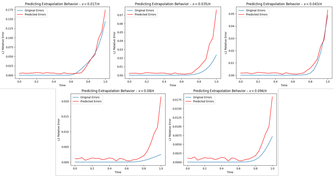
Given the observed relationship between Fourier spectra and extrapolation behavior, one may ask how well a reference solution’s Fourier spectra predict the extrapolation performance of a PINN. Towards answering this question, we train a vanilla PINN – MLP(4, 50) – on the Burger’s equation for different viscosities, equally spaced from to .
Given these learned solutions, we obtain relative L2 errors for each of the PDEs, comparing them to reference solutions obtained via numerical methods. Finally, we train a simple 4-layer MLP to predict the relative L2 errors for from the Fourier transforms of the reference solution at with standard MSE loss. For the purposes of numerical stability, we predict scaled errors, where all errors are multiplied by a factor of .
We withhold of the PDEs as a test set and evaluate the model’s performance on this set. To ensure that we have a representative test set, we use stratified sampling to split our range of viscosities into five contiguous regions, sampling one PDE from each region for the test set. Predictions are shown in Figure 25 for these PDEs, with the model achieving an of .
A.7 Multi-scale Fourier feature Networks
| Sigmas | Domain Loss | Boundary Loss | Int. Error | Ext. Error | Int. MAR | Ext. MAR |
|---|---|---|---|---|---|---|
| 1, 5 | 2.42e-4 | 2.95e-7 | 0.0026 | 0.7709 | 0.0057 | 1.6353 |
| 1, 10 | 5.35e-5 | 7.24e-7 | 0.0034 | 0.5612 | 0.0093 | 1.7226 |
| 1, 15 | 1.23e-4 | 3.07e-6 | 0.0272 | 0.5379 | 0.0289 | 2.0883 |
| 1, 5, 10 | 7.25e-5 | 5.19e-5 | 0.0156 | 0.7985 | 0.0127 | 2.2197 |
| No MFFN | 3.35e-5 | 1.66e-6 | 0.0031 | 0.5261 | 0.0082 | 1.1964 |
A.8 Effects of Transfer Learning on Interpolation & Extrapolation


| Setting | Int. Domain Loss | Int. Boundary Loss | Int. Combined Loss |
|---|---|---|---|
| Baseline | |||
| Transfer | |||
| Transfer |
| Setting | Ext. Domain Loss | Ext. Boundary Loss | Ext. Combined Loss |
|---|---|---|---|
| Baseline | |||
| Transfer | |||
| Transfer |
A.9 Investigations into Dynamic Pulling
We examine the improved extrapolation performance of the dynamic pulling method (DPM) proposed by Kim et al. 2020. In brief, their method modifies the gradient update in PINN training to dynamically place more emphasis on decreasing the domain loss in order to stabilize the domain loss curve during training.
We implement DPM for the Burgers’ equation with viscosity and compare to a standard PINN without DPM. For both sets of experiments, we use the architecture that Kim et al. 2020 found to have the best extrapolation performance on this particular PDE (MLP PINN with residual connections, 8 hidden layers, 20 hidden units per layer, tanh activation, and Xavier normal initialization). We train using Adam with learning rate and otherwise default parameters. When training with DPM, we use , , .

We train 77 DPM models and 60 standard models, differing only in the random seed. Our results are shown in Figure 28. As before, we find that our extrapolation error is dominated by the domain loss. Notably, we find that DPM on average does considerably worse in extrapolation than our baseline. However, the errors are higher variance and a number of DPM models perform better in extrapolation than any of our baseline models. The particular training dynamics induced by DPM which cause these shifts are unclear but potentially deserve more detailed investigation.
A.10 Training & Hardware Details
| Section | Model | Activation | Initialization | Optimizer | LR | Epochs | Samples |
| 3.1 (Figure 1) | MLP(4, 50) | Xavier | Adam | 1e-4 | 50000 | 10000, 40, 80 | |
| 3.2 (Figure 2) | MLP(4, 50) | (a), (b) | Xavier | Adam | 1e-4 | Varying | Varying |
| 4.1 (Figure 3) | MLP(3, 20) | Xavier | Adam | 1e-4 | 50000 | 10000, 40, 80 | |
| 4.2 (Figure 4) | MLP(6, 50) | Xavier | Adam | 1e-4 | 100000 | 20000, 80, 160 | |
| 5 (Figure 5) | MLP(5, 100) | Xavier | Adam | 1e-4 | Varying | Varying |
Hardware: All our experiments were conducted on an NVIDIA A100 GPU with 16 GB RAM.