PANTONE \AddSpotColorPANTONE PANTONE3015C PANTONE\SpotSpace3015\SpotSpaceC 1 0.3 0 0.2 \SetPageColorSpacePANTONE
Deep learning based Meta-modeling for Multi-objective Technology Optimization of Electrical Machines
Abstract
Optimization of rotating electrical machines is both time- and computationally expensive. Because of the different parametrization, design optimization is commonly executed separately for each machine technology. In this paper, we present the application of a variational auto-encoder (VAE) to optimize two different machine technologies simultaneously, namely an asynchronous machine and a permanent magnet synchronous machine. After training, we employ a deep neural network and a decoder as meta-models to predict global key performance indicators (KPIs) and generate associated new designs, respectively, through unified latent space in the optimization loop. Numerical results demonstrate concurrent parametric multi-objective technology optimization in the high-dimensional design space. The VAE-based approach is quantitatively compared to a classical deep learning-based direct approach for KPIs prediction.
Index Terms:
asynchronous machine, deep neural network, key performance indicators, multi-objective optimization, permanent magnet synchronous machine, variational auto-encoderI Introduction
Electrical machines play a pivotal role in the modern era, powering everything from home appliances to electric vehicles and industrial equipment. To reduce manufacturing costs, electrical machines are numerically optimized via virtual prototyping, which involves finite element (FE) simulations or analytical calculations before the actual machine is constructed.
Design evaluations using these classical techniques are both costly and time-consuming. Therefore, it is essential to find faster optimization methods to ensure a more sustainable and energy-efficient design workflow.
In recent years, there has been a significant increase in the use of machine learning-based meta-modeling for the accelerated numerical optimization of electrical machines for various purposes. For example, the study in [1] shows how trained data-driven deep learning (DL) models estimate magnetic field distribution for different low-frequency electromagnetic devices such as a transformer, a coil in air, and an interior permanent magnet machine. In another work [2], a convolutional neural network (CNN), a type of a deep neural network (DNN), is used as a meta-model for diagnosing stator winding faults of a permanent magnet synchronous machine (PMSM). The paper [3] presents how various machine learning methods assist in fault detection for induction machines. The concurrent application of variational autoencoder (VAE) and DNN for technology optimization of electromagnetic devices is investigated in [4]. An unsupervised learning-based anomaly detection model using a VAE for fault diagnosis in electric drive systems is presented in [5]. Several successful works of machine learning-based meta-modeling for the optimization of electromagnetic devices have been discussed in [6]. Many articles[7, 8, 9, 10, 11, 12, 13] demonstrate the successful application of different machine-learning approaches at different stages of the design and optimization of electrical machines. The reduction of computational time required to generate a sufficient amount of data for training large-scale machine learning-based meta-models needs to be addressed. In order to tackle this issue, a method is proposed in [14] for generating a large amount of data from a small number of FE simulation results using a deep generative model and a CNN. In a recent study [15], an approach for topology optimization of PM motors using the VAE and the neural network was demonstrated to generate various shapes and predict their corresponding motor characteristics within the optimization loop. However, the VAE often fails while reconstructing images in this approach. In [16], it has been shown how cross-domain key performance indicators (KPIs) can be estimated with high accuracy for different input representations of PMSM, i.e., image-based and parametric input using various DNNs. The parameter-based representation was observed to be more suitable concerning prediction accuracy with less computational effort than the image-based model. However, it can not deal with multiple topologies of PMSM concurrently. In [17], it is demonstrated how we can circumvent this problem for differently parameterized topologies of PMSM using VAE. The encoder maps the complex, high-dimensional combined input design space into a lower-dimensional unified latent distribution. In the latent space, multi-topology objective optimization was performed by predicting KPIs using DNN and generating associated new designs with the decoder.
So far, to the best of our knowledge, machine learning methods have been applied for a scenario dealing with the numerical optimization of a single machine type at a time, for example, PMSM, asynchronous machine (ASM), or DC machine. In this paper, we aim to perform concurrent multi-technology objective optimization (MTOO) for two different machine types, namely PMSM and ASM. Both machine types are distinctly parameterized and operate on different working principles. This difference can affect the performance and efficiency of the machines in various applications. For example, PMSMs typically have higher efficiency and power density than ASMs but may also be more expensive to manufacture due to the cost of the permanent magnets.
This paper proposes two significant differences compared to our previous works. We consider, in addition to geometric parameters, more challenging varying topological parameters such as pole pairs, number of slots per pole per phase, winding connection (star or delta), etc. Secondly, in order to handle these challenging parameters and the additional zeros in the combined design space, we propose a new optimization procedure that enhances synchronization between the decoder and the KPI predictor in the latent space. This proposed procedure improves the prediction accuracy of KPIs and associated design parameters. Additionally, we provide numerical analysis of the direct DL approach using a DNN for KPIs prediction[16].
The paper is organized as follows: in the next section, we explain the dataset details and training workflow. Section III discusses the network architecture and training details. Quantitative results are demonstrated in Section IV, and finally, the work is concluded in Section V.
II Dataset, training procedure and MOO
This section is divided into three subsections: the datasets detail, for explaining the VAE-based training workflow, and the last for formulating the multi-objective optimization (MOO) problem.
II-A Dataset
For the study, we build two datasets: one for an ASM and one for a PMSM. The usual industrial workflow of data generation is explained in Figure 3 for any electrical machine class. There may be some modifications in the workflow at the phase when the design evaluation is conducted. In this study, we evaluate a PMSM design with a time-intensive magneto-static FE simulation (see [18]), while the ASM design is evaluated with analytical calculations (see [19, 20]). The initial steps are identical in both instances of data generation. For example, specifying design parameters with constraints, creating a population with a Latin hypercube sampling technique [21] to cover the entire design space, and doing geometry checks for filtering erroneous designs using computer-aided design software (e.g.,[22]).
| KPIs | Value | |
|---|---|---|
| Material cost | Euro | |
| Maximum power | kW | |
| Maximum torque | Nm |
| System parameter | Value | Unit | |
|---|---|---|---|
| Inverter input DC voltage | 650 | V | |
| Inverter input DC current | 400 | A | |
| Rotational speed | (step size: 1000) | rpm |
II-A1 Dataset: ASM
| Input design parameter | Min | Max | Unit | |
| Stator outer diameter | 159 | 232 | mm | |
| Air gap | 0.65 | 1.7 | mm | |
| Rotor outer diameter | 85 | 190 | mm | |
| Rotor slot height | 10 | 21 | mm | |
| Rotor slot width | 0.6 | 1.5 | mm | |
| Discrete parameters | Value | Unit | ||
| Slots per pole per phase | [2-4] | - | ||
| Pole pairs (p) | [2-4] | - | ||
| Stator winding connection | star/delta | - | ||
| Winding scheme | short pitch/full pitch | - | ||
We selected valid ASM designs from the initial population. There is no fixed number of samples for data generation, but a large number of samples is usually preferred for the data-driven DL approach. There are total varying design parameters chosen for this data generation. From all the varying parameters, a few essential design parameters are detailed in Table III. Some parameters from Table III are shown in 2(a). Representative samples with varying pole pairs can be seen in Figure 1. 4(a) and 4(c) visualize distribution of the listed parameters and KPIs. The dataset contains topology changing parameters such as the number of slots per pole per phase , and varying pole pairs . Electrical parameters are included as design parameters, i.e., stator winding connection (star/delta) and winding scheme (short pitch/full pitch winding). The evaluation time for one design is about minutes on a single-core CPU.
II-A2 Dataset:PMSM
| Input design parameter | Min | Max | Unit | |
| Stator outer diameter | 159 | 232 | mm | |
| Rotor outer diameter | 100 | 197 | mm | |
| Air gap | 0.8 | 2.2 | mm | |
| Stator tooth height | 10 | 20 | mm | |
| Angle of magnet layer1 | 17 | 32 | mm | |
| Discrete parameters | Value | Unit | ||
| Slots per pole per phase | [2-4] | - | ||
| Pole pairs (p) | [3-5] | - | ||
| Stator winding connection | star/delta | - | ||
| Winding scheme | short pitch/full pitch | - | ||
We selected valid designs from the initial population. The number of samples for this dataset is close to the number of the previous ASM dataset (); otherwise, the network can be biased towards one machine technology during training. The number of varying design parameters for PMSM is . The PMSM dataset also incorporates variability for topological and electrical parameters. A few crucial parameters listed in Table IV can be observed in 2(b), and representative samples with the varying pole pairs are illustrated in Figure 1. The distribution of the listed parameters and KPIs is illustrated in 4(b) and 4(d), respectively.
Our goal is to perform concurrent multi-objective optimization for both technologies. Hence, both datasets were generated under the assumption of identical KPIs and constant system parameters. The KPIs and constant system parameters information are given in Table I and Table II, respectively. Furthermore, during data generation, it is assumed that the cost of standard materials (such as aluminium and copper) is the same for ASM and PMSM. The significant difference in cost comes when considering magnets for PMSM.
II-B Training procedure
We employ a VAE based workflow, it maps the input data to a low-dimensional latent space through a probabilistic encoder and then reconstructs it through a decoder[23]. As explained in [17], we first create a combined design space by concatenating the design vectors of all the given machines. It creates -dimensional design vector with , where represent input dimension of each different machine technology .
After concatenation, we define any th sample in the combined dataset as a dimensional vector if it is from the technology as
and KPIs vector for the design as
The total combined input dataset with all the machine types can be mathematically described by
| (1) |
The assumption is that dimensional unseen variables from a latent distribution can describe all the dimensional input samples from the dataset . It is also assumed that the input parameters of each machine type are independent of each other. Therefore, as described in [17], to reconstruct parameters with high accuracy, the latent dimension should be at least higher than the maximum input dimension of all the machine types, i.e., and also .
The encoder network computes the conditional distribution with the presumption that follows the standard normal distribution. It is written as
| (2) |
Where outputs mean () and diagonal component of the covariance matrix as a vector () represent latent distribution parameters with the dimension . are trainable encoder network () parameters.
To compute and backpropagate gradients during training, as described in [24], the latent vector is sampled using a reparametrization trick by
| (3) |
where is a noise vector, and is the component-wise dot product. The decoder network takes latent vector as input. It approximates the conditional distribution i.e.,
| (4) |
where are the trainable parameters of the decoder. Simultaneously, we train DNN with latent input () to predict the KPIs. It is written as
| (5) |
where are trainable parameters of the DNN and is vector of KPIs prediction. The primary goal of training the VAE is to minimize the errors in prediction, parameter reconstruction, and encoding process by optimizing the network parameters simultaneously. One important step of before training is defining the loss function. The choice of the training loss function depends on the specific task at hand. The MSE is commonly used as a loss function for regression tasks [25, Chapter 5], although other options, such as mean absolute error (MAE), exist. Through experiments, we determined that the MSE provides better prediction accuracy for our datasets. The MSE is a practical selection for parameter reconstruction since the input data is scalar. The total training loss comprises three components: the first two terms are squared error for parameter reconstruction and KPIs prediction, and the third term is Kullback-Leibler (KL) divergence for regularization in the latent space. Total VAE training loss is specified in terms of network parameters, input vector , and actual KPIs by The KL divergence minimizes the difference between encoder distribution and prior distribution over latent variables. It works as a regularizer term in the loss function to provide continuity and completeness in the latent space. It means the samples nearby in the latent space remain similar when decoded while preserving meaningful representation [26]. Here, for independent training of the DNN in a supervised manner[16] for each machine technology, we input as the input vector instead of latent vector . It is written as
| (6) |
Here, are network parameters, is the predicted KPIs vector, and is an input vector of the individual machine technology with dimension . The loss function during the network training is kept the same (MSE) as of the VAE for KPIs prediction. The only obvious change with the network structure is the input layer, compared to the used DNN during the VAE training. All the networks are trained using a standard back-propagation algorithm[27]. Figure 5 describes training workflow.
II-C MOO
Every electrical machine design optimization comprises many design variables, constraints, and competing objectives (see Table I). It leads to the generalized MOO problem formulation
| (7) | |||||
| s.t. | (8) | ||||
| (9) |
where represent input vector and and are parameter bounds, characterise KPIs, are constraints for design evaluation. Any commonly practiced multi-objective optimizer[28] can solve (7-9).
In this study, we propose two MOO workflows: one for MTOO via continuous latent space using VAE (see Figure 6) and another (Figure 7) for DNN-based classical workflow for individual machine technology.
In the VAE-based MTOO, randomly generated latent vector is input to the optimization process. As shown in Figure 6, first, we give the latent vector as input to the decoder(), and the decoder predicts design parameters for the related technology. From the data pre-processing, we have prior knowledge about the positions of the actual design parameters in the concatenated form of the input vector. Hence, we keep those values unchanged and fill the remaining values with zero except for the first entry. The first entry indicates technology type, so we replace the predicted continuous value with a known integer value. We also replace predicted discrete parameters, such as pole pairs, slots per pole per phase, winding scheme, known zero values etc., with integer values based on prior knowledge. This makes the input vector () in the form () that the encoder () expects. Then the encoder network creates a new latent vector , which is input to the KPIs predictor. The standard DNN-based MOO workflow (Figure 7) operates on one machine technology at a time, so we input a design vector with parameterization .
III Network architecture and Training specifications
III-A Network architecture
As illustrated in Figure 8, there are three networks: encoder (), decoder () and the DNN (). The network structure and training hyperparameters are obtained randomly through trial and error by evaluating approximately twenty configurations starting with the base network configuration from [17]. The details are as follows,
- •
Encoder network: The encoder() or inference network consists of four convolutional layers. These layers are significant for learning essential features from the combined design vector and determining whether the design is ASM or PMSM from the technology indicator (the first input parameter of the design vector). A flattened layer and a dense layer follow these convolutional layers. Three output layers follow the dense layer. Two output layers are the distribution parameters mean () and variance () that sample the final output latent vector ().
- •
Decoder network: The decoder network (), also called the generative network, consists of two dense layers, four convolution transposed layers, and one output layer corresponding to the dimension of the integrated design space. It follows the reverse structure of the encoder except for the output layer. The output layer has a linear activation function.
- •
DNN: The DNN is also interchangeably known as KPIs predictor in this study. The DNN has one input, five dense layers, and one output layer. For individual DNNs, we use an identical network structure (except the input layer) and hyperparameters, where we only train the DNN for one machine type at a time.
III-B Training specifications
| Parameters | Value |
|---|---|
| Learning rate | - |
| Total number of epochs | 300 |
| Validation patience | 20 |
| Optimizer | Adam[29] |
| Latent space dimension | 34 (as ) |
| Loss functions | KL-divergence and MSE |
| Batch size | 50 |
The total number of samples in a combined dataset is . We split a total number of samples () into three sets: training ( of ) , validation (), and testing (). Figure 9 displays training and validation curves. Table V gives the details of the training hyperparameters. The network training was carried out on NVIDIA Quadro M2000M GPU. It took hours to complete the VAE training for the multi-technology scenario, whereas separate DNNs takes around minutes with the for single machine technology. The magneto-static FE simulation takes h/sample for PMSM, and analytical calculation takes around minutes/sample for ASM on a single-core CPU.
IV Numerical results


| Prediction accuracy | ||||
| MAE | RMSE | PCC | MRE(%) | |
| 0.43 | 0.53 | 1 | 0.71 | |
| 1.90 | 2.54 | 1 | 1.31 | |
| 3.96 | 6.52 | 0.99 | 1.76 | |
| Parameters | Reconstruction accuracy | |||
|---|---|---|---|---|
| MAE | RMSE | PCC | MRE(%) | |
| Stator outer diameter | 0.39 | 0.483 | 0.99 | 0.19 |
| Air gap | 0.002 | 0.005 | 1 | 0.37 |
| Rotor outer diameter | 0.55 | 0.636 | 0.99 | 0.41 |
| Rotor slot height | 0.05 | 0.069 | 0.99 | 0.37 |
| Rotor slot width | 0.004 | 0.005 | 1 | 0.4 |
| Stator slot height | 0.05 | 0.004 | 1 | 0.32 |
| Parameters | Reconstruction accuracy | |||
| MAE | RMSE | PCC | MRE(%) | |
| Stator outer diameter | 0.51 | 0.63 | 0.99 | 0.26 |
| Rotor outer diameter | 0.39 | 0.5 | 0.99 | 0.27 |
| Air gap | 0.006 | 0.007 | 1 | 0.41 |
| Stator tooth height | 0.054 | 0.072 | 0.99 | 0.37 |
| Angle magnet layer 1 | 0.11 | 0.14 | 0.99 | 0.48 |
| Height of magnet layer 1 | 0.012 | 0.015 | 1 | 0.27 |
| Settings | Value |
|---|---|
| Sampling approach | random initialization |
| Population per generation | 1000 |
| Stopping criteria | 100 generations |
| Number of objectives | 2 |
| Crossover, mutation probability | 0.9 |
| KPIs | Design A (PMSM) | Design B (ASM) | ||||
|---|---|---|---|---|---|---|
| FE simulation | Prediction | MRE(%) | FE simulation | Prediction | MRE(%) | |
| 153.53 | 153.49 | 0.026 | 45.47 | 46.27 | 1.75 | |
| 402.98 | 406.70 | 0.92 | 241.7 | 237.82 | 1.60 | |
| 294.61 | 286.63 | 2.70 | 195.46 | 187.52 | 4.06 | |
| KPIs | Design C (PMSM) | Design D (ASM) | ||||
|---|---|---|---|---|---|---|
| FE simulation | Prediction | MRE(%) | FE simulation | Prediction | MRE(%) | |
| 130.81 | 129.51 | 0.99 | 46.68 | 46.73 | 0.53 | |
| 401.8 | 404 | 0.54 | 227.48 | 235 | 3.3 | |
| 313.05 | 316.27 | 1.02 | 158 | 200.36 | 26.81 | |
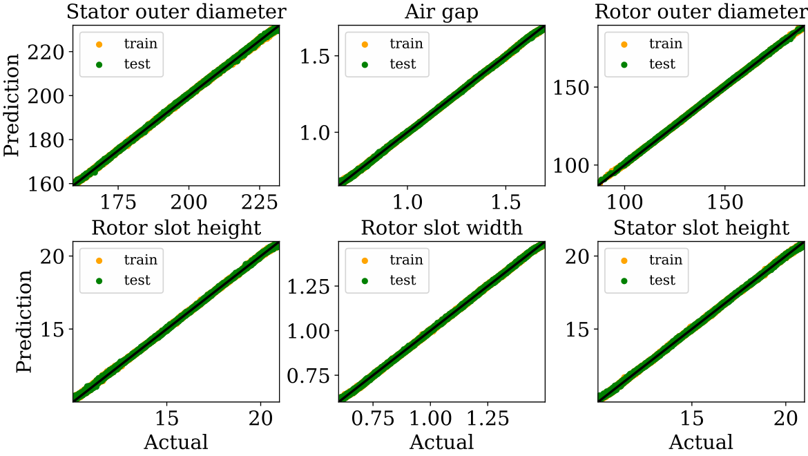
In this study, our primary focus is on the concurrent multi-technology scenario; therefore, we will explain the evaluation of the trained VAE in more detail. After training, we test trained models on the test dataset. Table VI gives evaluation details of test samples for all three global KPIs. We use unitless mean relative error (MRE), the root mean squared error (RMSE), MAE, and Pearson correlation coefficient (PCC) to measure the correlation between input and target variables. Figure 10 illustrates prediction plot of all these three KPIs over test samples. We can see that the maximum torque KPI () has a higher MAE ( Nm). We present a numerical analysis of parameter reconstruction of six parameters of each machine type in Table VII and Table VIII. It is observed that the parameter reconstruction is obtained with high precision. Figure 11 and Figure 12 display prediction plots. The other parameters, which are not illustrated here, also have higher reconstruction accuracy.
Figure 13displays a numerical comparison of the KPIs prediction performance of VAE and DNN with MAE over the same test samples. For the numerical analysis, the DNN is trained with a twin network configuration and hyperparameters as used for the DNN for the latent input. The DNNs are directly trained on the input parameters of each machine type, using a supervised learning approach. The VAE has a slightly better prediction accuracy than the trained DNN for the single machine types. This is likely due to more training samples in the combined dataset and more accurate functional mapping between latent input and output global KPIs.
The trained models (encoder, decoder and DNN) are used for MTOO for technologies. We propose an improved optimization workflow Figure 6. The proposed workflow improves synchronization between the decoder and the KPIs predictor in the optimization loop. It also handles many discrete input parameters effectively.
We perform MOO for two competing global KPIs: material cost and maximum power. We use the genetic algorithm NSGA-II, which can handle many design variables [28]. We set the MOO hyperparameters by experience; see Table IX for standard hyperparameters. The optimization process includes input parameter bounds as a constraint to reduce invalid design generation. The optimization requires roughly hours. We also run individual MOO for each machine type with the separately trained DNN model. Identical hyperparameter settings as of the VAE-based optimization are used. Each machine optimization takes around minutes. Figure 15 figure depicts different Pareto-fronts for the training samples, the VAE approach, and the separate DNN approach. All Pareto-fronts from DNNs and VAE show power or cost-effective designs. It can be seen that Pareto-fronts based on VAE and DNNs predictions contain designs that are not present in the training data. We illustrate two designs from each Pareto front. Design A (PMSM) and Design B (ASM) from the VAE Pareto front. Similarly, Design C (PMSM) and Design D (ASM) from the individually trained DNN models. We recalculated all these four designs with their conventional approach. Table X shows the evaluation for all three KPIs with MRE. We can see that Design B (ASM) has a high () MRE for maximum torque KPI. Likewise, Table XI evaluates Design C (PMSM) and D (ASM). For Design D, MRE is very high, , possibly due to a poor approximation of the meta-model for the maximum torque for that design. It is seen from Figure 15 that the DNN-based separate approach shows a more efficiently obtained Pareto front. We checked twenty designs from each Pareto front of both approaches. For the direct DNN-based approach, most designs from the more efficiently obtained Pareto region were found geometrically invalid. We observe that, even if we apply input parameter bounds as constraints to lower invalid design generation, we get much higher invalid designs () compared to VAE-based concurrent optimization. If the design is valid, then the prediction has a high deviation after recalculating with the conventional approach. Design D from Figure 15 is the example where we observe that recalculation produces a higher deviation in the prediction of torque KPI (MRE is ; see Table XI). This can be improved by adding geometry checks during optimization. However, that is beyond the scope of work.
V Conclusion and outlook
We present the application of the VAE-based approach for optimizing two different machine types (ASM and PMSM) simultaneously over a common set of KPIs, i.e., material cost and maximum power. The numerical results demonstrate high prediction accuracy for parameter reconstruction and KPIs in a complex design space. This enables the optimization of several electrical machine technologies with a single meta-model training. The quantitative analysis for the DNN-based direct approach for optimizing each machine type is also demonstrated. The MOO results show that direct DNN based approach has a more efficiently obtained Pareto region, but the VAE outputs more valid meaningful designs than independent optimization with DNN. However, the DNN-based optimization takes less computational effort than the VAE-based approach for fewer machines (in this study two). We expect a linear increase in the computational time during optimization for multiple machine types when the DNN-based models are trained separately. On the contrary, only a little increase in the computational time is expected for the VAE-based approach. Future work may include the application of trained meta-models in other query scenarios, such as sensitivity analysis and uncertainty quantification. The more challenging situation, e.g. optimization for more than two machine technologies, can also be considered.
References
- [1] Arbaaz Khan, Vahid Ghorbanian and David Lowther “Deep Learning for Magnetic Field Estimation” In IEEE Transactions on Magnetics 55.6, 2019, pp. 1–4 DOI: 10.1109/TMAG.2019.2899304
- [2] Przemyslaw Pietrzak, Marcin Wolkiewicz and Teresa Orlowska-Kowalska “PMSM Stator Winding Fault Detection and Classification Based on Bispectrum Analysis and Convolutional Neural Network” In IEEE Transactions on Industrial Electronics 70.5, 2023, pp. 5192–5202 DOI: 10.1109/TIE.2022.3189076
- [3] Stefan Quabeck, Wenbo Shangguan, Daniel Scharfenstein and Rik. De “Detection of Broken Rotor Bars in Induction Machines using Machine Learning Methods” In 2020 23rd International Conference on Electrical Machines and Systems (ICEMS), 2020, pp. 620–625 DOI: 10.23919/ICEMS50442.2020.9291033
- [4] Mauro Tucci, Sami Barmada, Alessandro Formisano and Dimitri Thomopulos “A Regularized Procedure to Generate a Deep Learning Model for Topology Optimization of Electromagnetic Devices” In Electronics 10.18, 2021 DOI: 10.3390/electronics10182185
- [5] Jaehoon Shim, Gyu Lim and Jung-Ik Ha “Unsupervised Anomaly Detection for Electric Drives Based on Variational Auto-Encoder” In 2022 IEEE Applied Power Electronics Conference and Exposition (APEC), 2022, pp. 1703–1708 DOI: 10.1109/APEC43599.2022.9773565
- [6] Paolo Di “Future Trends in Optimal Design in Electromagnetics” In IEEE Transactions on Magnetics 58.9, 2022, pp. 1–4 DOI: 10.1109/TMAG.2022.3164204
- [7] Liang Jin, Fei Wang and Qingxin Yang “Performance analysis and optimization of permanent magnet synchronous motor based on deep learning” In 2017 20th International Conference on Electrical Machines and Systems (ICEMS), 2017, pp. 1–5 DOI: 10.1109/ICEMS.2017.8056321
- [8] Haris Kurtović and Ingo Hahn “Neural Network Meta-Modeling and Optimization of Flux Switching Machines” In 2019 IEEE International Electric Machines & Drives Conference (IEMDC), 2019, pp. 629–636 DOI: 10.1109/IEMDC.2019.8785344
- [9] Saikou Cesay et al. “Generalizable DNN based multi-material Hysteresis Modelling” In 2022 IEEE 20th Biennial Conference on Electromagnetic Field Computation (CEFC), 2022, pp. 1–2 DOI: 10.1109/CEFC55061.2022.9940692
- [10] Armita Fatemimoghadam, Ye Yan, Lakshmi Iyer and Narayan. Kar “Permanent Magnet Synchronous Motor Drive Using Deep-Neural-Network-Based Vector Control for Electric Vehicle Applications” In 2022 International Conference on Electrical Machines (ICEM), 2022, pp. 2358–2364 DOI: 10.1109/ICEM51905.2022.9910710
- [11] Yu-Bai Yan et al. “Torque Estimation and Control of PMSM Based on Deep Learning” In 2019 22nd International Conference on Electrical Machines and Systems (ICEMS), 2019, pp. 1–6 DOI: 10.1109/ICEMS.2019.8921886
- [12] Akm Talukder, Bingnan Wang and Yusuke Sakamoto “Electric Machine Two-dimensional Flux Map Prediction with Ensemble Learning” In 2022 25th International Conference on Electrical Machines and Systems (ICEMS), 2022, pp. 1–4 DOI: 10.1109/ICEMS56177.2022.9982881
- [13] Maria Raia, Sebastian Ciceo, Fabien Chauvicourt and Claudia Martis “Multi-Attribute Machine Learning Model for Electrical Motors Performance Prediction” In Applied Sciences 13.3, 2023 DOI: 10.3390/app13031395
- [14] Yuki Shimizu, Shigeo Morimoto, Masayuki Sanada and Yukinori Inoue “Automatic Design System With Generative Adversarial Network and Convolutional Neural Network for Optimization Design of Interior Permanent Magnet Synchronous Motor” In IEEE Transactions on Energy Conversion 38.1, 2023, pp. 724–734 DOI: 10.1109/TEC.2022.3208129
- [15] Hayaho Sato and Hajime Igarashi “Fast Topology Optimization for PM Motors Using Variational Autoencoder and Neural Networks With Dropout” In IEEE Transactions on Magnetics 59.5, 2023, pp. 1–4 DOI: 10.1109/TMAG.2023.3242288
- [16] Vivek Parekh, Dominik Flore and Sebastian Schöps “Deep Learning-Based Prediction of Key Performance Indicators for Electrical Machines” In IEEE Access 9, 2021, pp. 21786–21797 DOI: 10.1109/ACCESS.2021.3053856
- [17] Vivek Parekh, Dominik Flore and Sebastian Schöps “Variational Autoencoder-Based Metamodeling for Multi-Objective Topology Optimization of Electrical Machines” In IEEE Transactions on Magnetics 58.9, 2022, pp. 1–4 DOI: 10.1109/TMAG.2022.3163972
- [18] Sheppard. Salon “Finite Element Analysis of Electrical Machines” Kluwer, 1995
- [19] Dieter Gerling “Induction Machines” In Electrical Machines: Mathematical Fundamentals of Machine Topologies Berlin, Heidelberg: Springer Berlin Heidelberg, 2015, pp. 135–188 DOI: 10.1007/978-3-642-17584-8˙4
- [20] Ion Boldea and Syed Nasar “The induction machines design handbook(2nd ed.)” CRC press, 2018 URL: https://doi.org/10.1201/9781315222592
- [21] M.D. Mckay, R.J. Beckkman and William Conover “Comparison of three methods for selecting values of input variables in the analysis of output from a computer code” In Technometrics 21, 2000, pp. 266–294 DOI: 10.1080/00401706.2000.10485979
- [22] Christophe Geuzaine and Jean-François Remacle “Gmsh: A 3-D finite element mesh generator with built-in pre-and post-processing facilities” In International journal for numerical methods in engineering 79.11 Wiley Online Library, 2009, pp. 1309–1331
- [23] Diederik. Kingma and Max Welling “An Introduction to Variational Autoencoders” In Foundations and Trends® in Machine Learning 12.4, 2019, pp. 307–392 DOI: 10.1561/2200000056
- [24] Diederik Kingma and Max Welling “Auto-Encoding Variational Bayes” In International Conference on Learning Representations, 2014
- [25] Ian Goodfellow, Yoshua Bengio and Aaron Courville “Deep Learning” http://www.deeplearningbook.org MIT Press, 2016
- [26] Alexander Amini and Ava Amini “MIT 6.S191: Introduction to Deep Learning” Lecture note, 2021 Massachusetts Institute of Technology URL: https://introtodeeplearning.com/
- [27] David. Rumelhart, Geoffrey. Hinton and Ronald. Williams “Learning representations by back-propagating errors” In nature 323.6088 Nature Publishing Group, 1986, pp. 533–536 DOI: 10.1038/323533a0
- [28] K. Deb, A. Pratap, S. Agarwal and T. Meyarivan “A fast and elitist multiobjective genetic algorithm: NSGA-II” In IEEE Transactions on Evolutionary Computation 6.2, 2002, pp. 182–197 DOI: 10.1109/4235.996017
- [29] Diederik. Kingma and Jimmy Ba “Adam: A Method for Stochastic Optimization” In International Conference on Learning Representations, 2015
![[Uncaptioned image]](2306.09087v3/fig/ieee_parekh.JPG) |
Vivek Parekh received his bachelor degree in electronics and communication from Gujarat technological university in 2012. He worked as an Assistant manager in Reliance Jio Infocomm Ltd. from 2013 to 2015 in operation and maintenance. He has obtained his M.Sc degree in information technology from the University of Stuttgart in 2019. Currently, he is pursuing a Ph.D. at TU Darmstadt in the Institut für Teilchenbeschleunigung und Elektromagnetische Felder under the fellowship of Robert Bosch GmbH. His area of interest comprises machine learning, deep learning, reinforcement learning, optimization of electrical machine design, and the industrial simulation process. |
![[Uncaptioned image]](2306.09087v3/fig/ieee_flore.JPG) |
Dominik Flore received the bachelor in maschinenbau with specialization in mechatronik and master in maschinenbau with specialization in Product development from the University of Paderborn in 2012 and 2013, respectively. He obtained a Ph.D. degree with the topic ”Experimentelle Untersuchung und Modellierung des Schädigungsverhaltensfaserverstärkter Kunststoffe” from ETH Zürich, in 2016. Currently, he is working as a development engineer for the reliability of the electric machine at Robert Bosch GmbH, Stuttgart. Present research interests involve product development in the field of electrical machine with the application of machine learning, optimization of the industrial simulation process. |
![[Uncaptioned image]](2306.09087v3/fig/ieee_schoeps.jpg) |
Sebastian Schöps received the M.Sc. degree in business mathematics and a joint doctoral degree from the Bergische Universität Wuppertal and the Katholieke Universiteit Leuven in mathematics and physics, respectively. He was appointed a Professor of computational electromagnetics with the Technische Universität Darmstadt within the interdisciplinary centre of computational engineering in 2012. Current research interests include coupled multiphysical problems, bridging computer aided design and simulation, parallel algorithms for high performance computing, digital twins, uncertainty quantification and machine learning. |