Fast and Examination-agnostic Reciprocal Recommendation in Matching MarketsConference: Seventeenth ACM Conference on Recommender Systems; September 18–22, 2023; Singapore, SingaporeSeventeenth ACM Conference on Recommender Systems (RecSys ’23), September 18–22, 2023, Singapore, SingaporeDOI: 10.1145/3604915.3608774ISBN: 979-8-4007-0241-9/23/09CCS: Information systems Recommender systemsCCS: Information systems Social recommendationCCS: Applied computing Economics
Abstract.
In matching markets such as job posting and online dating platforms, the recommender system plays a critical role in the success of the platform. Unlike standard recommender systems that suggest items to users, reciprocal recommender systems (RRSs) that suggest other users must take into account the mutual interests of users. In addition, ensuring that recommendation opportunities do not disproportionately favor popular users is essential for the total number of matches and for fairness among users. Existing recommendation methods in matching markets, however, face computational challenges on real-world scale platforms and depend on specific examination functions in the position-based model (PBM). In this paper, we introduce the reciprocal recommendation method based on the matching with transferable utility (TU matching) model in the context of ranking recommendations in matching markets, and propose a faster and examination-agnostic algorithm. Furthermore, we evaluate our approach on experiments with synthetic data and real-world data from an online dating platform in Japan. Our method performs better than or as well as existing methods in terms of the total number of matches and works well even in relatively large datasets for which one existing method does not work.
Keywords:
Matching Markets, Reciprocal Recommender Systems (RRSs), Matching Theory1. Introduction
In matching markets, such as job posting and online dating platforms, reciprocal recommender systems (RRSs) play a crucial role in the success of the platforms (Pizzato et al. 2010; Mine et al. 2013). Unlike conventional recommender systems that suggest items to users, RRSs that suggest other users need to take into account two aspects that do not appear in conventional recommender systems. First, recommendation results need to be based on the mutual preferences of users. In job posting platforms, for example, even if one job seeker has a strong interest in one job post, the employer might not be interested at all in the job candidate; the “match” between the job seeker and the employer will not be established in this case. Therefore, recommending job posts to a job seeker only according to the seeker’s interest is not effective, and hence RRSs should recommend only when both users are mutually interested. Second, recommendation opportunities should not concentrate on a few popular users. The number of matches that one user can make is often physically limited because it is impossible for one employer to have interviews with all candidates. Thus, distributing match opportunities widely among users is important to maximize the total number of matches, and fairness among users is important in matching markets.
To take into account the first aspect (i.e., the mutuality of preferences), most reciprocal recommendation methods aggregate two unilateral preference scores (of job candidates toward employers and vice versa) into a bilateral preference score via some aggregate functions. Unilateral preference scores can be generally calculated by standard recommendation methods such as matrix factorization (Hu et al. 2008; Koren et al. 2009). Arithmetic mean, geometric mean, or harmonic mean are typically used as the aggregate function in the literature and in practice. However, most of the aggregate functions do not reflect the second aspect, the necessity of avoiding concentration on a few popular users, and this issue has not been analyzed enough in the literature.
To tackle this issue, Su et al. 2022 recently consider the problem of ranking recommendation in the matching markets, including job posting platforms. They define the social welfare function as the expected total number of matches and propose a method to choose a stochastic ranking recommendation policy that maximizes the approximate social welfare function. In the experiment simulating a matching market, their method substantially improves the total number of matches compared to both the naive method based on naive unilateral preferences and the reciprocal method based on the product of two unilateral preferences. However, there are still two practical challenges to using Su et al. 2022’s method in real-world platforms. First, their method involves a doubly stochastic matrix, whose size is quadratic in the number of users in the reactive side (e.g., employers), for each proactive side user (e.g., job candidates) as variables, and solves a convex optimization problem with constraints. In real-world scale matching platforms, it is very expensive to directly solve the convex optimization problem of such sizes in terms of both space and time complexity. In addition, implementing the stochastic ranking recommendation is challenging because the Birkhoff–von-Neumann decomposition (Birkhoff 1946) of doubly stochastic matrices for each proactive user is also computationally prohibitive. Second, their method depends on the specific form of the examination functions in the position-based model (PBM). In PBM, the examination function maps a ranking that an item listed on to a probability with which a user has attention to the item. Although some methods to estimate the examination function are proposed, it is still hard in practice to estimate it correctly because the examination functions are specific to each application and may be different among individual users. Su et al. 2022 use an examination function for both the objective function to optimize in their method and the evaluation via Monte Carlo simulations, and they do not consider the problem of misspecification of examination functions.
In the literature on the matching theory (Gale and Shapley 1962; Roth and Sotomayor 1992), economists and computer scientists have developed various matching algorithms that seek to match two sides of agents appropriately according to the mutual preferences of agents and their matching capacity, which correspond to two aspects of RRSs discussed above. Especially, matching with transferable utility (TU matching) models (Shapley and Shubik 1971) have been developed to analyze the job markets (Kelso Jr. and Crawford 1982) and the marriage markets (Becker 1973; Becker 1974; Choo and Siow 2006). In these models, monetary transfers are assumed to occur between two agents matched, and the amounts of transfers are adjusted so as to balance the demands from both sides in the matching market, just as prices in the standard economic markets. The resulting matching, which is called “equilibrium matching” in this paper, reflects the mutuality of preferences and avoids the concentration of matching on a few popular people, and thus it would be effective to apply it in the reciprocal recommendations.
In this paper, we consider the reciprocal recommendation method based on the TU matching model of Choo and Siow 2006, in the setting of the ranking recommendation in the matching markets. Our proposed TU method computes a deterministic ranking policy more efficiently in terms of both space and time complexity than Su et al. 2022’s method, and it is independent of a form of the examination function.
The contribution of this paper is as follows. First, in the setting of ranking recommendation in the matching markets, we propose a reciprocal recommendation method based on TU matching model and develop an efficient algorithm. Second, we evaluate our TU method in experiments with synthetic data and real-world data from an online dating platform in Japan, comparing with baselines including SW method of Su et al. 2022. Our TU method performs at least as well as SW method in terms of the expected total number of matches, and outperforms the conventional RRS methods such as Naive and Reciprocal methods. Moreover, TU method outperforms SW with the misspecified examination function in most cases, and it also works well even in relatively large datasets where SW method does not work.
1.1. Related work
Reciprocal recommendation
Of particular distinction in reciprocal recommendation from the standard item recommendation is that a system must consider the bilateral preferences of proactive and reactive users. Most of the conventional methods estimate the preferences of each side of users by using a corresponding model and then use the bilateral preference estimates to predict a reciprocal preference. As the first step of unilateral preferences can be solved by standard recommender methods, modeling reciprocal preferences is often reduced into the aggregation of bilateral preferences. In this context, various aggregation functions have been proposed, e.g., arithmetic mean (Neve and Palomares 2019b; Neve and Palomares 2019a), geometric mean (Neve and Palomares 2019b; Neve and Palomares 2019a), harmonic mean (Pizzato et al. 2010; Xia et al. 2015), cross-ratio uniform (Appel et al. 2017), matrix multiplication (Jacobsen and Spanakis 2019), the multiplicative inverse of rank multiplication (Mine et al. 2013), and weighted mean with optimized weighting parameters (Kleinerman et al. 2018). Neve and Palomares 2019b proposed an early method that optimizes two independent matrix factorization models of unilateral preferences and then aggregates two preference estimates using arithmetic, geometric, or harmonic means. However, such aggregation functions highly depend on the scale and domain of unilateral preference estimates and lack a theoretical foundation. By contrast, recent fairness-aware recommendation do not consider such aggregation functions by directly maximizing a welfare function (Do et al. 2021; Do and Usunier 2022).
Inefficiency issues in post-processing approach based on doubly stochastic matrices
Fairness-aware methods based on the post-processing approach often rely on the post-estimation of doubly stochastic matrices, which represent stochastic recommendation policies for users (Singh and Joachims 2018; Do et al. 2021; Usunier et al. 2022; Do and Usunier 2022; Saito and Joachims 2022; Su et al. 2022). Methods in this category may be impractical due to the quadratic computational cost with respect to the number of items for each user. Recent methods alleviate this issue by using Frank-Wolfe algorithms that enable efficient parameter updates in the quasi-linear cost with respect to the number of items for each user (Do et al. 2021; Do and Usunier 2022). The practical implementation of probabilistic ranking systems is also challenging because the pre-computation step for sampling a ranked list from a doubly stochastic matrix can be costly due to the Birkhoff–von-Neumann decomposition (Birkhoff 1946), which involves iteratively finding a perfect matching on the matrix. Moreover, although the main interest of conventional studies is the fairness guarantee for algorithms, most of the provable guarantee does not hold in practice as the availability of the true preferences and true examination probabilities is often assumed.
Matching theory and reciprocal recommendations based on matching theory
Our methodology builds upon the literature of matching theory (Roth and Sotomayor 1992; Manlove 2013) originated by Gale and Shapley 1962, which has been widely applied to a variety of applications, including hospital-resident assignment (Roth and Peranson 1999; Kamada and Kojima 2015), school matching (Abdulkadiroğlu et al. 2005b; Abdulkadiroğlu 2005; Abdulkadiroğlu et al. 2005a), and paper-reviewer assignment (Lian et al. 2018; Garg et al. 2010; Stelmakh et al. 2021). Especially, the matching with transferable utility model (TU model) (Shapley and Shubik 1971; Chiappori 2017) considers matching markets where agents matched can transfer utility or money between them. Economists have applied the TU matching models to analyze the job market (Kelso Jr. and Crawford 1982) and the marriage market (Becker 1973; Becker 1974). Choo and Siow 2006 develops an empirical model of the marriage market and applies it to the empirical study of the real marriage market in the US, and several works have developed its generalized model and estimation algorithms (Decker et al. 2013; Galichon and Salanié 2022).
Although there are a few studies that apply the matching theory literature to the problem of reciprocal recommendation (Saini et al. 2019; Eskandanian and Mobasher 2020; Pizzato and Silvestrini 2011), the interaction of reciprocal recommendation and matching theory has been relatively less analyzed. The most similar work to this paper in terms of methodology is Chen et al. 2023, which considers recommending users based on the equilibrium matching of Choo and Siow 2006 model in online dating. However, the main method that they use in the online experiment separates users into several groups and estimates preferences for each group, and thus it does not correspond directly to the fully personalized recommendation11 1 Chen et al. 2023 also considers personalized recommendation that built on preferences estimated via MF in offline experiments in the appendix of their paper, but their experimental setting is limited and its impact on the total number of matches is not analyzed enough.. In addition, the main issue that they consider is the inequality of matching opportunities among users rather than the total number of matches. Tomita et al. 2022 also discuss the reciprocal recommendation method based on Choo and Siow 2006 model, but they did not describe the whole algorithm of the method and did not evaluate the performance in any experiments. In this paper, we propose a fully-personalized reciprocal recommendation method based on TU matching of Choo and Siow 2006 model in the framework of ranking recommendation in matching markets (Su et al. 2022), and evaluate its performance in terms of the total number of matches in experiments with synthetic data and real-world data.
| notation | description |
|---|---|
| set of job candidates | |
| set of job posts | |
| estimated preference score of candidate to employer | |
| estimated preference score of employer to candidate | |
| set of all possible ranked lists of employers | |
| a deterministic ranking policy of each job candidate | |
| a stochastic ranking policy is a mapping from a candidate | |
| examination function, e.g., or | |
| employer ’s rank in the ranked list | |
| candidate ’s rank in employer ’s list (when applied to ) | |
| probability that candidate applies to employer | |
| probability that employer matches to candidate | |
| social welfare of stochastic ranking policy | |
| a doubly stochastic matrix with size of for reduced from |
2. Setup
In this section, we introduce a framework for ranking recommendations in matching markets according to Su et al. 2022, and several re-ranking methods such as the naive, reciprocal, and social welfare maximization (Su et al. 2022). Table 1 lists the notations frequently used in this paper.
2.1. Framework for recommendation in matching markets
Following Su et al. 2022, we describe the framework of matching markets in the context of job posting platforms. This framework can be applied to other matching markets such as online dating platforms. In this market, job candidates (proactive side) first browse a list of ranked job posts/employers and apply to the ones they are interested in. The employer (reactive side) receives a list of job candidates who applied to them and then selects the ones he/she considers qualified for the job.
We now present a formal model of this market. Let be the set of job candidates, and be the set of job posts or employers. We note that both sets are finite (). Each candidate has a preference over the set of job posts , and each employer has a preference over the candidate set .
Although the platform does not know the true preferences of job candidates and employers, we assume that their estimations are available by using some recommendation methods. Let be the estimated preference of candidate to employer , and be that of to . The score can be thought of as the probability with which has relevance with conditioning that examined ; a similar analogy can be applied to .
The platform can choose a ranked list of employers sent to each job candidate. Let be the set of all possible ranked lists of employers . A deterministic ranking policy is a mapping from each job candidate to a ranked list of employers that is sent to the candidate . A stochastic ranking policy is a mapping from a candidate to a probability distribution of ranked lists of employers . In this work, we study how to design deterministic ranking policies (the naive, reciprocal, and our methods mentioned below), while the focus of Su et al. 2022 is on stochastic ranking policies. We also note that a deterministic ranking policy is a special case of stochastic ranking policies that take ranking for each candidate with probability , and thus we explain the framework and objective in terms of stochastic policies for simplicity below.
After obtaining a ranked list of employers , each candidate chooses whether to apply for each employer. In this framework, we use the position-based model (PBM) (Joachims et al. 2017). Conditioning on the ranked list , the probability with which the candidate applies to an employer is
where is the rank of the employer in the ranked list , and is an examination function, that is, is a probability with which the candidate examines the employer positioning on rank . Typically, or are used. With a stochastic ranking policy , the probability with which a candidate applies to an employer , denoted by can be calculated as below:
| (1) |
After the application process by the job candidates, each employer receives the list of candidates who applied to the employer . The list is sorted in descending order according to the employer’s preference , beforehand by the platform. Employers examine the lists and then choose candidates to “match”, that is, to get in touch with or to conduct an interview with. As in the case of job candidates, we also use the PBM for this employer’s process. The probability with which the employer matches to conditioning on that applied to , denoted by is
where is a rank of in the list for the employer conditioning on the policy and that applied to . We note that is a random variable even if is deterministic because it relies on the set of candidates who also applied for the employer .
Given a policy , the social welfare is defined as the expected total number of matches (Su et al. 2022):
| (2) |
The platform’s objective is to find an appropriate policy such that the social welfare is maximized.
2.2. Existing methods
Given the matching market explained above, we highlight popular existing methods, the naive methods, reciprocal methods, and the approximate social welfare maximization approach (Su et al. 2022).
Naive method
One of the most popular methods in practice is to re-rank employers naively according to job candidates’ preferences. For each job candidate , let be the ranked list of employers , which is sorted in descending order according to the candidate ’s preference score .
Reciprocal method
Many works in the RRSs use aggregation functions that aggregate two unilateral scores into a reciprocal score to take into account the mutuality of preferences. One of the most popular aggregation functions is the geometric mean, or equivalently in terms of the order, the product of job candidates’ and employers’ preference scores (Neve and Palomares 2019a; Neve and Palomares 2019b). In the reciprocal method, the platform provides the job candidate with the ranked list of employers which is sorted in descending order according to the reciprocal scores .
Approximate social welfare maximization (Su et al. 2022)
Unlike the naive and reciprocal methods, the approximate social welfare maximization method (Su et al. 2022) optimizes a stochastic policy directly. The probability (1) with which candidate applies to employer in a stochastic policy can be expressed as:
| (3) |
where is the doubly stochastic matrix reduced from , that is, is the probability with which the employer is ranked at position for the candidate in the stochastic policy . In the PBM, the probability with which applies to relies only on the position where the employer is displayed and preference score , and not on other employers’ position. Therefore, the application probability (3) can be expressed in terms of the doubly stochastic matrix reduced from the stochastic policy .
Then the social welfare (2) is:
| (4) |
However, the social welfare (4) cannot be directly optimized because the rank of in ’s list depends on other candidates’ applications and thus the term is too complex to tackle with. Su et al. 2022 derive a lower bounds of under the assumption of convexity of examination function :
| (5) |
where . They propose the SW method that optimizes this approximated social welfare instead of :
| (6) |
Several approaches can be used to solve the convex optimization problem (6). Su et al. 2022 use the Frank-Wolfe approach, which is summarized as Algorithm 1.
However, there are some practical difficulties in implementing this social welfare optimization approach in real-world matching markets as discussed in Section 1. The objective function (5) includes the true examination function , whose estimation is hard in practice. Moreover, materializing the doubly stochastic matrices for all candidates is unrealistic due to its computational cost of for each timestep, and the precomputation for efficient sampling of rankings from a doubly stochastic matrix involves Birkhoff–von-Neumann decomposition, which is very costly to solve for all job candidates; we further discuss this point in Section 3.2.
3. TU matching approach
In this section, we propose a reciprocal recommendation algorithm based on the matching with transferable utility (TU matching) model. In Section 3.1, we introduce Choo and Siow 2006’s model of TU matching and explain the concrete algorithm. In addition, we develop a practical inference implementation using efficient vector search algorithms (Shrivastava and Li 2014) in Section 3.2, which is contrast to existing stochastic methods that need pre-computation of Birkhoff-von Neumann decomposition in inference time.
3.1. TU matching model
In the model discussed below, we interpret that estimated preference scores and are the estimation of surplus or gains that they obtain when they match with each other. When the candidate and the employer match, they split surplus
where and are the estimation error of preferences , respectively, which are assumed to be identically and independently distributed from some probability distribution . In the TU matching model, we assume that monetary transfer occurs between a job candidate and an employer when they are matched. Transfers are interpreted in physical markets as, for example, wages in the job market, household sharing in the marriage market, or gifts in dating markets. Although there may not be such explicit transfers between users on online platforms, we assume that some implicit transfers occur and use virtual transfers as a tool to derive an appropriate matching. Let be the transfer amount that the employer gives to when they match. In this case, the candidate /the employer obtains
from the matching, respectively. In this matching market, each agent chooses one that maximizes his/her gain from the set of opponents. They also have an outside option, or remaining “unmatched” in this market, which is denoted as “”. The stochastic demand of the candidate toward the employer , that is, the probability with which chooses is
| (7) |
and the stochastic demand of the employer toward (the probability with which chooses ) is
| (8) |
where we assume , and i.i.d. for any .22 2 The existence of an outside option is not a crucial assumption because the model and method can be written and derived without the outside option “”. We contain following the tradition of matching with transferable utility literature (Choo and Siow 2006) and for the simplicity of notation and method.
The equilibrium is a situation where both sides of stochastic demands coincide by the transfers’ adjustment, just as the market price in the standard physical market, which adjusts demands and supplies. We call the adjusted transfers and (fractional) matching as equilibrium matching.
Definition 0.
An equilibrium matching satisfies the following conditions:
- (1)
satisfies
(9) (10) - (2)
equals both sides of demands:
for all .
The intuition of the equilibrium matching in TU matching model is as follows. For a popular candidate , is generally high for many employers, and the demands of employers toward (8) likely to exceed the demands of toward employers (7). In this case, transfers that the candidate requests to employers increase to adjust the excess demands in the market. On the other hand, a popular employer with high s tends to have excess demands from many candidates. In this case, to adjust the excess demand toward , the market would decrease that the employer needs to pay when he matches. After these adjustment processes, demands from both sides are settled in equilibrium. Economists consider that the equilibrium is achieved in real-world matching markets such as job markets or marriage markets, and analyzes this equilibrium matching in TU matching model. Online matching markets might also suffer from the excess demands toward a few popular users. Therefore, we consider that the equilibrium in TU matching would be effective in designing a desirable reciprocal recommendation that takes into account two aspects discussed in the Introduction: the mutuality of preferences and the avoidance of concentration on a few popular users.
Galichon and Salanié 2022 show that the equilibrium matching exists, can be computed as a solution to a convex optimization problem, and maximizes social gains under constraints. However, solving this equilibrium matching, in general, is computationally difficult. To derive tractable equations of equilibrium matching, we introduce the Gumbel specification (Choo and Siow 2006) of preference errors’ distribution.
Assumption 1.
Estimation errors of preference scores ( for each , and for each ) are identically and independently distributed from the Gumbel (type-I extreme value) distribution with location and scale .
Given Assumption 1, we can show that for each in equilibrium is
| (11) |
where is the stochastic demand of / toward the outside option . In our method, we compute this equilibrium matching and generate the ranked list of employers in the descending order of to each candidate . Unlike standard reciprocal recommendation methods that use aggregate functions, such as the product function discussed Section 2.2, the equilibrium matching (11) is computed with not only the preference scores between the two users, but also with determined by the overall balance of the market.
Now we can derive a system of equations to find the equilibrium matching. Let and . The equilibrium matching satisfies the following system of equations:
| (12) | ||||
| (13) | ||||
| (14) |
The derivation of these equations is shown in Appendix A.1.
These equations can be solved in several methods. In our experiments discussed later, we solve the equations via IPFP (Iterative Proportional Fitting Procedure) (Decker et al. 2013; Galichon and Salanié 2022), which is summarized as Algorithm 2.
3.2. Computational efficiency in inference time
As mentioned above, the existing method requires precomputing Birkhoff–von-Neumann decomposition (Birkhoff 1946) of a doubly stochastic matrix for each job candidate to efficiently sample a deterministic ranking in inference time. However, it leads to a prohibitively large computational cost, being infeasible in realistic applications. The space cost for the precomputed set of top- deterministic rankings for each job candidate may also be impractical. By contrast, our method enables efficient real-time retrieval via vector search algorithms (Shrivastava and Li 2014) when employing two-tower/dot-product models (Rendle et al. 2020), such as matrix factorization (Hu et al. 2008; Koren et al. 2009), for preference scores; this is an essential property for large-scale applications (e.g., (Covington et al. 2016)). Assume that preference scores can be expressed in the following dot-product models,
Here, and are the -dimensional feature mappings for job candidates in the two preference models, while and are those for job posts. Recall here that our method predicts a ranked list of for a candidate according to the order of , and hence it is equivalent to use to generate ranked lists due to the monotonicity of . By using Equation (11), this equivalent ranking score can be reformulated as follows:
where is the concatenation of two vectors and . Therefore, our method maintains the desirable structure in dot-product models of preference scores by using the following -dimensional feature mappings,
Note here that we omitted the positive constant as it does not affect ranking predictions.
4. Experiments with synthetic data
In this section, we report experimental results that compare our proposed method with other methods on synthetic datasets33 3 The codes are available at https://github.com/CyberAgentAILab/tu-matching-recommendation.. The experiment setup in this section strictly follows Su et al. 2022.
4.1. Setup
Data generation
We generated synthetic data according to the setup of Su et al. 2022. The number of employers is and that of job candidates is where is the market size parameter in .
To simulate various scenarios, we divide each unilateral preference score into two terms: and for each , where the first term is the overall popularity of the user, and is its weight representing the degree of crowding. Here, employers and job candidates are indexed as , and we ensure that employers/candidates with low indexes are generally popular with all candidates/employers, i.e., for each , and for each . The second term is the individual preference of each user. We independently and identically draw from uniform distribution . The crowding level in the market is controlled by the crowding parameter . We consider three types of examination functions , i.e., (i) “inv”: , (ii) “exp”: , and (iii) “log”: . Unless mentioned, we use , , and (i.e., “inv”) for all users in the experiments.
Metrics
We evaluate our method and baselines in terms of the expected total number of matches , which is defined by Equation (2). We estimate it by Monte Carlo simulations of the interaction processes in the matching market, which is described in Section 2.1. For each setting, we repeatedly run this experiment 10 times and report the average results.
Methods compared
We compare our TU method with three baselines, Naive, Reciprocal, and SW (Su et al. 2022) methods, which are discussed in Section 2.2. We set learning rate and timesteps for the SW method following Su et al. 2022. For our TU method, we use . We also tested other values of , but the results are similar to the case of . The detail for effects of is discussed in Appendix A.2. In all cases, we confirmed that the IPFP algorithm converges in less than steps44 4 We decide that the procedure has converged if both updates of all in one step and errors of the constraints (9)–(10) have become less than 1e-9..
4.2. Results


Market sizes
We test for various market sizes , and . The results are reported in Fig. 3. Although the total number of matches in all methods increases when the market size grows, the comparison results are almost unaffected by the market size. TU outperforms Naive and Reciprocal methods, and performs as well as SW method. We note that SW cannot be computed for the case of , and hence we do not report its result for this case, which corresponds to the rightmost figure. In addition, since the variation in the 10 experiments is very small and the standard errors are on the order of 1e-1, the error bars are extremely small or invisible in Fig 3, which is also the case in Fig. 3 and Fig. 3.
Crowding
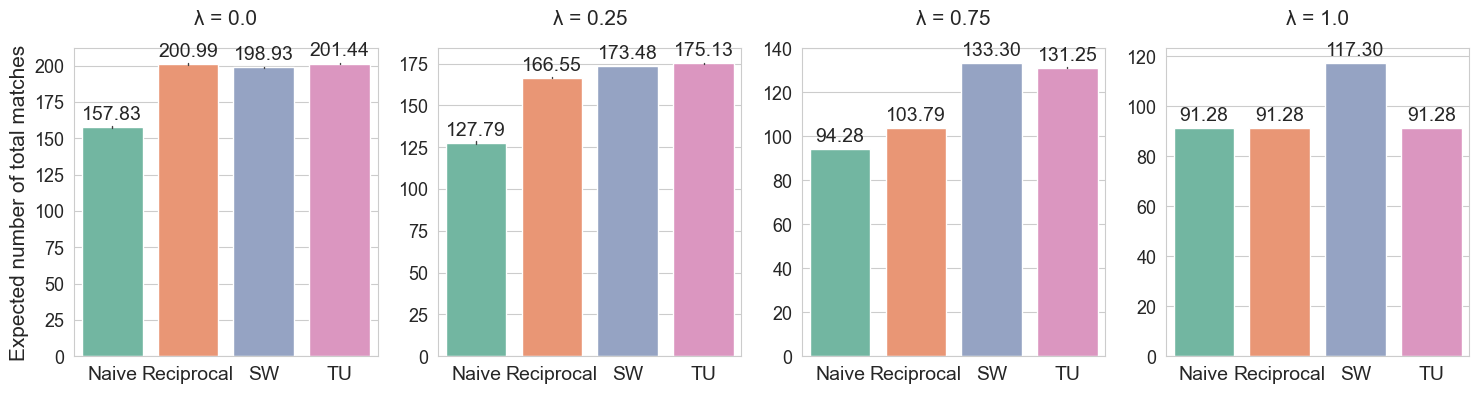
We also test for various levels of crowding , , , , and . The results are shown in Fig. 3. The case of equals the case of in Fig. 3, and thus it is omitted in Fig. 3. With lower crowding parameter , which means that users’ preferences vary and there are few inequalities of popularity among users, TU is as well as Reciprocal and SW. On the other hand, in the case of , which means that there are huge inequalities of popularity among users, TU performs worse than SW. In the middle level of crowding , TU outperforms Naive and Reciprocal while it performs as well as SW.
Examination functions
Finally, we test three types of examination functions (log, inv, and exp) used in the Monte Carlo simulations in the testing phase. In addition, to assess the effect of misspecification of examination functions used in SW discussed in Section 2.2, we consider the variants of SW with different examination functions in the training phase, namely, SW_log, SW_inv, and SW_exp, which use log, inv, and exp examinations in the objective of SW, respectively. Market size is , and the crowding parameter is . The results are reported in Fig. 3. In each case, the SW variants with misspecified examination functions (e.g., SW_inv and SW_exp in the log case) perform worse than the SW with correct examination functions. Specifically, SW_exp underperforms even Reciprocal method in the log case, and SW_log in the exp case performs 17.7 % worse than SW_exp. By contrast, TU is competitive to SW with correct examinations in log and inv cases and slightly deteriorates in the exp case. In most cases, TU outperforms SW with misspecified examination functions, whereas it slightly underperforms SW_inv in the exp case.
Summary
In summary, we show in these synthetic experiments that:
- (1)
TU method performs as well as SW method in many cases.
- (2)
It works well even in relatively large datasets for which SW does not work, and substantially outperforms the conventional Naive and Reciprocal methods.
- (3)
It outperforms SW methods with misspecified examination functions in many cases, except that SW_inv in the exp case; however, the performance gap between SW_inv and TU is not substantial.
In real-world platforms, it is often difficult to specify the examination function for each user accurately, and SW is also infeasible even in the case with . Therefore, our TU method would be effective in practice.
5. Experiments with real-world data
We conducted an experiment using real-world data collected from an online dating platform. This service is a Japanese online dating platform with millions of cumulative members, where men are recommended to women and vice versa. Users who receive recommendations choose “like” if they prefer the other person and “dislike” if they do not. Furthermore, users who receive “like” respond with “thank you” if they like the other person and “sorry” if they do not. Only when a “thank you” is received does the match become established. Then they will be able to chat.
5.1. Setup
Data preprocessing
We explain how to create moderate-sized data using our raw, large data. We first extracted two datasets, one consisting of sampled men and women (denoted dataset) and the other consisting of sampled men and women (denoted dataset). Our preliminary experiments revealed that the baseline method of Su et al. 2022 did not work on the dataset due to its space and time complexity, whereas Monte Carlo simulations and our proposed method work. Hence, we used the additional dataset for comparison between our algorithm and the baselines.
Since random sampling may yield too sparse data to train MF-based preference models, we performed the following two steps to extract a subset of users that induces a dense component: In the first step, we filtered users by their residence. The intuition behind this filtering is that users are more likely to prefer each other if they are living in the same (or nearby) residence. In the second step, we applied a -core decomposition algorithm to the remaining data. For a graph , a -core is any maximal subgraph of such that every vertex has degree at least (Seidman 1983)55 5 In our dataset, each vertex corresponds to a user, and each edge represents an interaction between a pair of uses.. Therefore, a -core (with large ) is able to find a dense part of . It should be noted that there are two directions of interaction due to the service’s specifications: (1) male-proactive scenario: men receiving a “thank you” for their “like” from women, and (2) female-proactive scenario: women receiving a “thank you” for their “like” from men. For pairs with unobserved evaluation data, we used the Alternating Least Squares (ALS) method to complete the data.
Experimental process
To assess the performance of our method with real-world data, we conducted the Monte Carlo simulations as well as synthetic data simulations discussed in Section 4. Using the estimated preferences from real-world data discussed above, we ran Naive, Reciprocal, TU, and SW (only for the dataset) methods. We used constant learning rate and timesteps for the learning process of SW, and for TU, similarly to the synthetic data experiments. We used the inv examination function for both the Monte Carlo simulations and the objective function of SW. We estimated the expected total number of matches by running Monte Carlo simulations times for datasets, and times for datasets.
5.2. Results

The results are reported in Fig. 4. TU method performs slightly worse than SW, and as well as Reciprocal in datasets for both male-proctive and female-proactive case. We note that the inv examination function is used both for the objective function of SW and the Monte Carlo simulation process and the issue of misspecification of is not considered in this simulation, and thus it is just an infeasible skyline method. In datasets, TU performs clearly better than Naive and Reciprocal methods.
As in the synthetic experiments, we show in these experiments with real-world data that the TU method is also effective for realistic situations. These results suggest that our TU method would be beneficial in practice for real-world online dating or job posting platforms with more than thousands of users.
6. Conclusions and Future works
In this paper, we introduce the TU matching-based reciprocal recommender system that does not rely on the specific form of examination functions, and works in a relatively large datasets for which one existing method does not work. We evaluate the performance of our method in experiments with synthetic and real-world data from an online dating platform. Our TU method outperforms the conventional Naive and Reciprocal methods, and performs at least as well as the SW method. These experiments suggest that the TU method can be superior to SW in a realistic situation where SW uses a possibly misspecified examination function.
There are several considerable future directions in the field of reciprocal recommendation in matching markets. First, in this paper, whereas we evaluate our TU method only in experiments that run Monte Carlo simulations that simulate the matching markets, evaluation in online A/B experiments in real-world platforms remains for future works. Moreover, it is also important to develop offline/off-policy evaluation methods in reciprocal recommendation in matching markets.
Next, more scalable ranking methods in RRSs would also be a future direction. Although our TU method is more efficient in terms of time and space complexity than the Su et al. 2022’s method, it still costs the order of computational complexity for each timestep in Algorithm. 2, and we only conduct experiments with datasets at most. Since there are real-world matching platforms with tens or hundreds of thousands of users, a more efficient implementation of our TU method or other algorithms would be needed for such large-scale matching platforms.
Another future direction is applications of other matching algorithms. Besides TU matching (Shapley and Shubik 1971; Choo and Siow 2006; Galichon and Salanié 2022), many other matching algorithms have been developed in the field of matching with non-transferable utility (NTU matching), such as the differed acceptance (DA) algorithm of Gale and Shapley 1962. Only a few works have developed a reciprocal recommender system based on matching algorithms like DA algorithm (Saini et al. 2019; Eskandanian and Mobasher 2020; Pizzato and Silvestrini 2011). Especially, there seems to be possible interaction between the issues of fairness in the reciprocal recommendation and the matching with constraints. In the literature of matching theory, various algorithms with complex constraints regarding fairness issues have been recently developed, such as NTU matching with affirmative actions (Abdulkadiroğlu 2005; Hafalir et al. 2013) and with regional constraints (Kamada and Kojima 2015; Aziz et al. 2020), and TU matching with regional constraints (Jalota 2022; Matsushita et al. 2022). These matching algorithms with constraints could be beneficial to improve the fairness of reciprocal recommendations.
Finally, the issues of incentive and strategic behavior in reciprocal recommendation would also be an important future direction. In reciprocal recommendations, the problem could be whether users act according to their true preferences. For example, a job seeker may not apply for a job slot in which she is strongly interested because the position seems to be popular among job seekers and highly competitive. Thus, the action history obtained in reciprocal recommendations may not reflect the true preferences of users. Furthermore, consider the situation where the reciprocal recommendation method other than the naive method that recommends naively according to the estimated preferences of proactive users is used. Users may have incentives to manipulate their actions and reveal false preferences because the recommendation systems do not simply suggest users that they seem to be interested in. The issue of strategic behavior has been extensively analyzed in matching theory, and many “strategy-proof” matching algorithms that incentivize users to reveal their true preferences have been developed (Roth and Sotomayor 1989; Sönmez 1994). Designing RRSs that incentivize users to act according to their true preferences based on strategy-proof matching algorithms could be an interesting future direction.
Appendix A Appendix
| Method | Naive | Reciprocal | SW | TU | |||||
|---|---|---|---|---|---|---|---|---|---|
| # of matches | 106.450 | 129.824 | 152.269 | 152.318 | 152.365 | 152.389 | 152.460 | 152.722 | 153.089 |
| (0.176) | (0.178) | (0.101) | (0.104) | (0.104) | (0.105) | (0.096) | (0.102) | (0.095) | |
| # of iterations | 39 | 39 | 40 | 42 | 48-49 | >100,000 | |||

A.1. Derivation of Equations in IPFP
Given Assumption 1 and transfers , the stochastic demands of candidates (7) and employers (8) can be written as
| (15) |
for each (here we note that ) and
| (16) |
for each (also note that ). In the equilibrium matching , we can derive
| (17) |
where the first equality holds because (7)–(8) in the equilibrium and the second equality holds since (15)–(16). Let and . Combining (17) with constraints (9)–(10), we have the equations (12)–(14).
A.2. Effects of
The only hyperparameter that needs to be tuned in the Algorithm 2, other than timesteps or stopping criterion, is the scale parameter for the Gumbel distribution of preference errors in Assumption 1. To evaluate the effects of on the performance of the TU method, we test and for the case of , , and (inv) in the synthetic data experiments. The results are reported in Table 2. Although larger results in slightly better performances in terms of the expected total number of matches, it seems that values of do not have a large impact on performances. However, the number of iterations needed for convergence increases when increases. Especially, the procedure did not converge even after iterations for , where we report the performance of after iterations.
A.3. Discussion on Fairness
In matching markets such as job posting and online dating platforms, not only is the total number of matches important but also the fairness between users. In addition, it may be effective even for the total number of matches to distribute matches fairly among users rather than to concentrate matches to a few popular users. The two left graphs in Fig. 5 show the Gini index of matches among candidates and employers in synthetic experiments in the case of , , and the inv examination function. The mean of 10 simulations is reported. A lower Gini coefficient indicates a more equal distribution. In the two right graphs, the distributions of matches among candidates and employers in one representative simulation are shown. In both graphs, we can see that TU is as fair as SW, and fairer than Naive and Reciprocal methods. Especially, the equality of matches among employers (reactive side) substantially improves in TU and SW methods from Naive and Reciprocal methods.
References
- (1)
- Abdulkadiroğlu (2005) Atila Abdulkadiroğlu. 2005. College admissions with affirmative action. International Journal of Game Theory 33 (2005), 535–549.
- Abdulkadiroğlu et al. (2005a) Atila Abdulkadiroğlu, Parag A Pathak, and Alvin E Roth. 2005a. The new york city high school match. American Economic Review 95, 2 (2005), 364–367.
- Abdulkadiroğlu et al. (2005b) Atila Abdulkadiroğlu, Parag A Pathak, Alvin E Roth, and Tayfun Sönmez. 2005b. The Boston public school match. American Economic Review 95, 2 (2005), 368–371.
- Appel et al. (2017) Orestes Appel, Francisco Chiclana, Jenny Carter, and Hamido Fujita. 2017. Cross-ratio uninorms as an effective aggregation mechanism in sentiment analysis. Knowledge-Based Systems 124 (2017), 16–22.
- Aziz et al. (2020) Haris Aziz, Serge Gaspers, Zhaohong Sun, and Toby Walsh. 2020. From matching with diversity constraints to matching with regional quotas. arXiv preprint arXiv:2002.06748 (2020).
- Becker (1973) Gary S. Becker. 1973. A theory of marriage: Part I. Journal of Political Economy 81, 4 (1973), 813–846.
- Becker (1974) Gary S. Becker. 1974. A theory of marriage: Part II. Journal of Political Economy 82, 2, Part 2 (1974), S11–S26.
- Birkhoff (1946) Garrett Birkhoff. 1946. Three observations on linear algebra. Univ. Nac. Tucumán, Rev. Ser. A 5 (1946), 147–151.
- Chen et al. (2023) Kuan-Ming Chen, Yu-Wei Hsieh, and Ming-Jen Lin. 2023. Reducing recommendation inequality via two-sided matching: A field experiment of online dating. International Economic Review (2023).
- Chiappori (2017) Pierre-André Chiappori. 2017. Matching with transfers: The economics of love and marriage. Princeton University Press.
- Choo and Siow (2006) Eugene Choo and Aloysius Siow. 2006. Who Marries Whom and Why. The Journal of Political Economy 114, 1 (2006), 175–201.
- Covington et al. (2016) Paul Covington, Jay Adams, and Emre Sargin. 2016. Deep neural networks for YouTube recommendations. In RecSys. 191–198.
- Decker et al. (2013) Colin Decker, Elliott H. Lieb, Robert J. McCann, and Benjamin K. Stephens. 2013. Unique equilibria and substitution effects in a stochastic model of the marriage market. Journal of Economic Theory 148, 2 (2013), 778–792.
- Do et al. (2021) Virginie Do, Sam Corbett-Davies, Jamal Atif, and Nicolas Usunier. 2021. Two-sided fairness in rankings via Lorenz dominance. In NeurIPS. 8596–8608.
- Do and Usunier (2022) Virginie Do and Nicolas Usunier. 2022. Optimizing generalized Gini indices for fairness in rankings. In SIGIR. 737–747.
- Eskandanian and Mobasher (2020) Farzad Eskandanian and Bamshad Mobasher. 2020. Using stable matching to optimize the balance between accuracy and diversity in recommendation. In UMAP. 71–79.
- Gale and Shapley (1962) David Gale and Lloyd S. Shapley. 1962. College admissions and the stability of marriage. The American Mathematical Monthly 69, 1 (1962), 9–15.
- Galichon and Salanié (2022) Alfred Galichon and Bernard Salanié. 2022. Cupid’s Invisible Hand: Social Surplus and Identification in Matching Models. The Review of Economic Studies 89, 5 (2022), 2600–2629.
- Garg et al. (2010) Naveen Garg, Telikepalli Kavitha, Amit Kumar, Kurt Mehlhorn, and Julián Mestre. 2010. Assigning papers to referees. Algorithmica 58 (2010), 119–136.
- Hafalir et al. (2013) Isa E. Hafalir, M. Bumin Yenmez, and Muhammed A. Yildirim. 2013. Effective affirmative action in school choice. Theoretical Economics 8, 2 (2013), 325–363.
- Hu et al. (2008) Yifan Hu, Yehuda Koren, and Chris Volinsky. 2008. Collaborative filtering for implicit feedback datasets. In ICDM.
- Jacobsen and Spanakis (2019) Anik Jacobsen and Gerasimos Spanakis. 2019. It’s a Match! Reciprocal Recommender System for Graduating Students and Jobs. In EDM. 580–583.
- Jalota (2022) Devansh Jalota. 2022. Matching with transfers under distributional constraints. arXiv preprint arXiv:2202.05232 (2022).
- Joachims et al. (2017) Thorsten Joachims, Adith Swaminathan, and Tobias Schnabel. 2017. Unbiased Learning-to-Rank with Biased Feedback. In WSDM. 781–789.
- Kamada and Kojima (2015) Yuichiro Kamada and Fuhito Kojima. 2015. Efficient matching under distributional constraints: Theory and applications. American Economic Review 105, 1 (2015), 67–99.
- Kelso Jr. and Crawford (1982) Alexander S. Kelso Jr. and Vincent P. Crawford. 1982. Job matching, coalition formation, and gross substitutes. Econometrica: Journal of the Econometric Society (1982), 1483–1504.
- Kleinerman et al. (2018) Akiva Kleinerman, Ariel Rosenfeld, Francesco Ricci, and Sarit Kraus. 2018. Optimally balancing receiver and recommended users’ importance in reciprocal recommender systems. In RecSys. 131–139.
- Koren et al. (2009) Yehuda Koren, Robert Bell, and Chris Volinsky. 2009. Matrix factorization techniques for recommender systems. Computer (2009).
- Lian et al. (2018) Jing Wu Lian, Nicholas Mattei, Renee Noble, and Toby Walsh. 2018. The conference paper assignment problem: Using order weighted averages to assign indivisible goods. In AAAI, Vol. 32.
- Manlove (2013) David Manlove. 2013. Algorithmics of matching under preferences. Vol. 2. World Scientific.
- Matsushita et al. (2022) Akira Matsushita, Kei Ikegami, Kyohei Okumura, Yoji Tomita, and Atsushi Iwasaki. 2022. Regulating Matching Markets with Constraints: Data-driven Taxation. arXiv preprint arXiv:2205.14387 (2022).
- Mine et al. (2013) Tsunenori Mine, Tomoyuki Kakuta, and Akira Ono. 2013. Reciprocal recommendation for job matching with bidirectional feedback. In IIAI-AAI. 39–44.
- Neve and Palomares (2019a) James Neve and Ivan Palomares. 2019a. Aggregation strategies in user-to-user reciprocal recommender systems. In SMC. 4031–4036.
- Neve and Palomares (2019b) James Neve and Ivan Palomares. 2019b. Latent factor models and aggregation operators for collaborative filtering in reciprocal recommender systems. In RecSys. 219–227.
- Pizzato et al. (2010) Luiz Pizzato, Tomek Rej, Thomas Chung, Irena Koprinska, and Judy Kay. 2010. RECON: A Reciprocal Recommender for Online Dating. In RecSys. 207–214.
- Pizzato and Silvestrini (2011) Luiz Augusto Pizzato and Cameron Silvestrini. 2011. Stochastic matching and collaborative filtering to recommend people to people. In RecSys. 341–344.
- Rendle et al. (2020) Steffen Rendle, Walid Krichene, Li Zhang, and John Anderson. 2020. Neural collaborative filtering vs. matrix factorization revisited. In RecSys. 240–248.
- Roth and Peranson (1999) Alvin E Roth and Elliott Peranson. 1999. The redesign of the matching market for American physicians: Some engineering aspects of economic design. American Economic Review 89, 4 (1999), 748–780.
- Roth and Sotomayor (1989) Alvin E. Roth and Marilda Sotomayor. 1989. The college admissions problem revisited. Econometrica: Journal of the Econometric Society (1989), 559–570.
- Roth and Sotomayor (1992) Alvin E. Roth and Marilda Sotomayor. 1992. Two-sided matching. Handbook of Game Theory with Economic Applications 1 (1992), 485–541.
- Saini et al. (2019) Amar Saini, Florin Rusu, and Andrew Johnston. 2019. PrivateJobMatch: A privacy-oriented deferred multi-match recommender system for stable employment. In RecSys. 87–95.
- Saito and Joachims (2022) Yuta Saito and Thorsten Joachims. 2022. Fair Ranking as Fair Division: Impact-Based Individual Fairness in Ranking. In KDD. 1514–1524.
- Seidman (1983) Stephen B. Seidman. 1983. Network Structure and Minimum Degree. Social Networks 5, 3 (1983), 269–287.
- Shapley and Shubik (1971) Lloyd S. Shapley and Martin Shubik. 1971. The assignment game I: The core. International Journal of Game Theory 1, 1 (1971), 111–130.
- Shrivastava and Li (2014) Anshumali Shrivastava and Ping Li. 2014. Asymmetric LSH (ALSH) for sublinear time maximum inner product search (MIPS). In NIPS. 2321–2329.
- Singh and Joachims (2018) Ashudeep Singh and Thorsten Joachims. 2018. Fairness of exposure in rankings. In KDD. 2219–2228.
- Sönmez (1994) Tayfun Sönmez. 1994. Strategy-proofness in many-to-one matching problems. Economic Design 1 (1994), 365–380.
- Stelmakh et al. (2021) Ivan Stelmakh, Nihar Shah, and Aarti Singh. 2021. PeerReview4All: Fair and Accurate Reviewer Assignment in Peer Review. Journal of Machine Learning Research 22, 163 (2021), 1–66.
- Su et al. (2022) Yi Su, Magd Bayoumi, and Thorsten Joachims. 2022. Optimizing Rankings for Recommendation in Matching Markets. In WWW. 328–338.
- Tomita et al. (2022) Yoji Tomita, Riku Togashi, and Daisuke Moriwaki. 2022. Matching Theory-based Recommender Systems in Online Dating. In RecSys. 538–541.
- Usunier et al. (2022) Nicolas Usunier, Virginie Do, and Elvis Dohmatob. 2022. Fast online ranking with fairness of exposure. In FAccT. 2157–2167.
- Xia et al. (2015) Peng Xia, Benyuan Liu, Yizhou Sun, and Cindy Chen. 2015. Reciprocal recommendation system for online dating. In ASONAM. 234–241.