VIBR: Learning View-Invariant Value Functions for Robust Visual Control

Tom Dupuis Affiliation: Universite Paris-Saclay, CEA, List, F-91120, Palaiseau, France ´ Affiliation: U2IS, ENSTA Paris, Institut Polytechnique de Paris, Palaiseau, France Jaonary Rabarisoa Affiliation: Universite Paris-Saclay, CEA, List, F-91120, Palaiseau, France ´ Quoc-Cuong Pham Affiliation: Universite Paris-Saclay, CEA, List, F-91120, Palaiseau, France ´ David Filliat Affiliation: U2IS, ENSTA Paris, Institut Polytechnique de Paris, Palaiseau, France Affiliation: INRIA FLOWERStom.dupuis@cea.fr

Abstract

End-to-end reinforcement learning on images showed significant progress in the recent years. Data-based approach leverage data augmentation and domain randomization while representation learning methods use auxiliary losses to learn task-relevant features. Yet, reinforcement still struggles in visually diverse environments full of distractions and spurious noise. In this work, we tackle the problem of robust visual control at its core and present VIBR (View-Invariant Bellman Residuals), a method that combines multi-view training and invariant prediction to reduce out-of-distribution (OOD) generalization gap for RL based visuomotor control. Our model-free approach improve baselines performances without the need of additional representation learning objectives and with limited additional computational cost. We show that VIBR outperforms existing methods on complex visuo-motor control environment with high visual perturbation. Our approach achieves state-of the-art results on the Distracting Control Suite benchmark, a challenging benchmark still not solved by current methods, where we evaluate the robustness to a number of visual perturbators, as well as OOD generalization and extrapolation capabilities.

1 Introduction

Learning policies that are invariant to visual distractions is crucial for the usage of reinforcement learning for real-world visuomotor control problems. The visual variance of the real world is practically unbounded and the distribution of possible events has an extremely heavy tail. For example, end-to-end autonomous driving struggles with the never-ending list of edge cases sparsely present in the data. Although there is real progress in visual generalization in robotic manipulation for example, we are quite far from reaching human levels of robustness.

Data augmentation is extensively used for building inductive biases in pure computer vision tasks, such as image classification. One can not imagine reaching state-of-the-art performance on usual benchmarks without using a careful combination of transformation on images. In particular, pretraining representations with teacher-student self-supervised objectives is a popular and successful method. Such architecture usually enforces invariance of representations to different augmentations of the same image. As such, multiple works take inspiration from success in computer vision and build methods to learn visual invariances for control and reinforcement learning (Yarats et al. 2020).

In the case of classification, invariance of representations is a reasonably efficient optimization strategy, as classifying images from pretrained representations is relatively straightforward and only require linear probing in most cases. Because classifying the content of an image is a semantically high level task, the class label is resilient to a lot of intense visual transformation of the image. Features such as exact position, relative organization and textures of entities in the image are usually not predictive of the class label. Data augmentation for implicit invariance is straightforward to apply in these cases and computer vision pipelines fully take advantage of this fact.

In the case of control, however, finding a meaningful and useful policy from a given state representation is multiple orders of magnitude more complex than assigning a class token. Small visual changes in images might necessitate very different action decisions, which means policies must be sensitive to high-frequency variations in images. This goes against principles of data augmentation in computer vision tasks like classification where invariances holds for very aggressive augmentations. The problem gets worse when policies are implemented with deep neural networks, which are known to learn over low-frequency components of the data (Rahaman et al. 2019). This directly suggests that any representational approximation error will directly impact the upper-bound performance of the policy. The problem is slightly mitigated with discrete action which theoretically allow partial mode collapse of observations in the latent space, but continuous control represents a serious challenge.

Figure 1: Evaluation metrics at the end of training aggregated over all 5 curriculum benchmarks and 6 tasks of the Distracting Control Suite, 21 episodes and 4 seeds each. See section 4 for details.

From this observation, we present View-Invariant Bellman Residuals (VIBR) for robust visuomotor control under visual distractions. Importantly, our approach does not require a representation learning self-supervised loss and directly performs invariant prediction, which we show is a relaxed constraint that enables better optimization and performances. We show that VIBR is able to efficiently train an agent with visual generalization capabilities without losing on convergence speed and asymptotic performance on the original task. In particular, we derive a view-invariant temporal-difference loss combining multi-view empiricial risk minimization with variance regularization. We show that view-invariant prediction can serve as a powerful inductive bias for learning robust policies and value functions with reinforcement learning, even under intense perturbations. Our main contributions are:

•

a novel methodology for robust visuomotor control based on temporal-difference learning on images using invariant prediction principles
•

empirical results on the Distracting Control Suite benchmark (Stone et al. 2021) with state-of-the-art results on raw training performance (Figure 1) and out-of-distribution (OOD) generalization under the hardest setting of dynamic distractions
•

a fair comparison with competitive baselines of invariant representation learning for RL
•

an analysis of the influence of inter-view variance regularization in learning dynamics

2 Context and Problem Setting

We first details the context and notations, then position ourselves compared to representation learning and introduce the tools of risk minimization.

2.1 Value-Based Reinforcement Learning

Markov Decision Process and RL:

We define the Markov Decision Process $\mathcal{M}=\langle\mathcal{S},\mathcal{A},P,R,\gamma\rangle$ where $S$ is the set of states, $A$ the set of actions, $P:\mathcal{S}\times\mathcal{A}\rightarrow\mathcal{S}$ the transition probability function, $R:\mathcal{S}\times\mathcal{A}\times\mathcal{S}\rightarrow\mathbb{R}$ the reward function and $\gamma$ a discounting factor for discriminating between short-term and long-term rewards. We also define the transition tuple containing state, action, reward and next state as $T=(s,a,r,s+)$ where $a\sim\pi$ , $s+\sim P^{\pi}(s+|s)$ is the successor state of $s$ and $r\sim R(s,a,s+)$ the reward. In this setting, reinforcement learning aims to maximize the total reward received by the agent. Mathematically, it corresponds to finding a policy $\pi$ that maximizes the (discounted) expected return $\mathbb{E}_{T\sim\pi,P^{\pi}}[\sum_{t=0}^{\infty}\gamma^{t}r_{t}]$ .

Bellman operator and Bellman error:

Value-based algorithms for control estimate the (state-action) value function $Q^{\pi}$ which is defined for every state $s_{t}$ : $Q^{\pi}(s_{t},a_{t})=\mathbb{E}_{\pi}\left[\sum_{k=0}^{+\infty}\gamma^{k}r_{k+t+1}\right]$ with $r_{k+t+1}=R(s_{t},a_{t},s+)$ . We will use the notation $Q(s,\pi)=\mathbb{E}_{a\sim\pi}\left[Q(s,a)\right]$ for simplicity. This connects the state value function to the state-action value function: $V^{\pi}(s)=Q(s,\pi)$ . We can define the Bellman evaluation operator $\mathcal{T}^{\pi}$ :

\mathcal{T}^{\pi}Q^{\pi}(s,a)=r(s,a)+\gamma\mathbb{E}_{s+\sim P^{\pi}(s+|s)}Q(s+,\pi)

(1)

We define the Bellman error and Bellman residuals:

(\mathcal{B}^{\pi}Q)(s,a)=Q^{\pi}(s,a)-\mathcal{T}^{\pi}Q^{\pi}(s,a)

(2)

\mathcal{L}_{\mathrm{BR}}=\mathbb{E}_{T}\left[\lvert\lvert(\mathcal{B}^{\pi}Q)(s,a)\rvert\rvert^{2}\right]

(3)

2.2 Observations and Representations

Observer:

We assume the Block-MDP setting as defined by Du et al. 2019.

Definition 2.1.

BlockMDP A block MDP is the tuple $\mathcal{M_{x}}=\langle\mathcal{S},\mathcal{A},\mathcal{O},P,x,R,\gamma\rangle$ which is an extension of the MDP defined above where $\mathcal{O}$ is an observation space (potentially much bigger than $\mathcal{S}$ ) and $x:\mathcal{S}\rightarrow\mathcal{O}$ is a ”context-emission function” or observer.

The observer $x$ is responsible for generating observation for each state of the system but is most of the time unknown. We equip the Block MDP with the following assumption:

Assumption 2.1.

Block structure Each observation $o$ uniquely determines its generating state $s$ . That is, the observation space $\mathcal{O}$ can be partitioned into disjoint blocks $O_{s}$ , each containing the support of the conditional distribution $x(\cdot|s)$ (Du et al. 2019).

This ensures that for a given BMDP $\mathcal{M}_{x}$ , the corresponding observer $x$ is well-defined and injective and guarantees non-ambiguity of observations This assumption gives us the Markov property and makes $\mathcal{M}_{x}$ a proper MDP on which we can work and use all the existing results of RL.

We now have a constructive method to define multiple views or observations of a single state. All it requires is to sample multiple observers but otherwise keeping other elements of the MDP constant. Given a list of observers $\left[x^{1},...,x^{K}\right]$ , we have a list of MDPs $\left[\mathcal{M}_{x^{1}},...,\mathcal{M}_{x^{K}}\right]$ to train on. Importantly, each of these MDP share the same reward function, dynamics and state and action space and thus encode the same exact task. If the environments are run in parrallel, this provides extremely rich information to extract invariance to observers, as the hidden state at each step is equal over all environments. Finding optimal policies is then only a matter of information retrieval from observations and should be theoretically possible with any view.

Representation learning:

Numerous works take a different view to robustness on visual variations and focus on guiding the parameters of the value network with the help of auxiliary tasks (Jaderberg et al. 2017; Bellemare et al. 2019; Dabney et al. 2021). In this context, the approximated value function can be decomposed with a representation network $\phi$ and a linear layer $w$ : $Q^{\pi}_{\theta}(s,a)=\phi(s,a)\cdot w$ ¹¹ 1 Note that we could arbitrarily choose the representation layer to be earlier than the penultimate layer and the linear layer would become a shallow non-linear network, but this will not change our argument.

Representation learning aims to learn $\phi$ with some auxiliary objectives to better condition the space of value functions to accelerate learning and/or improve generalization. With online reinforcement learning, the agent is trained on both RL and (self-supervised) representation learning objectives at the same time: $\mathcal{L}_{\mathrm{tot}}=\mathcal{L}_{\mathrm{aux}}(\phi)+\mathcal{L}_{\mathrm{RL}}(\phi,w)$ where $\mathcal{L}_{\mathrm{aux}}$ is the (self-supervised) representation loss and $\mathcal{L}_{\mathrm{RL}}$ is the RL loss.

2.3 Multi-Domain Training

We are interested in training value functions that are robust to out-of-distribution domain shifts for robust visual control. Given $K$ domains $\mathcal{D}^{k}$ , we can define the empirical risk associated to each domain as the expectation of a loss function $l$ on this domain: $\mathcal{R}(\mathcal{D}^{k};\theta)=\mathbb{E}_{X\sim\mathcal{D}^{k}}[l(X;\theta)]$ where $X$ is the training data containing individual samples and $\theta$ is the parameters of the model being trained. A simple approach is to perform Empirical Risk Minimization (ERM), i.e. averaging risks on training domains:

\theta^{\ast}\in\min\sum_{k}\lvert\mathcal{D}^{k}\rvert\mathcal{R}(\mathcal{D}^{k};\theta)

(4)

This approach doesn’t guarantee transfer under OOD conditions. Given different domains $\left[\mathcal{D}^{1},...\mathcal{D}^{K}\right]$ , it is possible to minimize the ERM objective by overfitting on one particular domain $\mathcal{D}^{k}$ while not optimizing a lot over other domains, let alone unknown domains. To prevent that, it is possible to use constraint optimization to force equality of training risks across domains:

\min_{\theta}\sum_{k}\lvert\mathcal{D}^{k}\rvert\mathcal{R}(\mathcal{D}^{k};\theta)\quad\textrm{s.t.}\quad\forall(k,l)\in[1...K]\times[1...K]\quad\mathcal{R}(\mathcal{D}^{k};\theta)=\mathcal{R}(\mathcal{D}^{l};\theta)

(5)

The constraint of perfect equality of risk is equivalent to enforcing variance of risks to zero:

\min_{\theta}\quad\sum_{k}\lvert\mathcal{D}^{k}\rvert\mathcal{R}(\mathcal{D}^{k};\theta)\quad\textrm{s.t.}\quad\mathrm{Var}(\mathcal{R}(\mathcal{D}^{k};\theta))=0

(6)

This hard constraint can then be relaxed with a soft convex penalty facilitating optimization, leading to the V-REx approach (Krueger et al. 2021):

\min_{\theta}\quad\sum_{k}\lvert\mathcal{D}^{k}\rvert\mathcal{R}(\mathcal{D}^{k};\theta)+\beta\mathrm{Var}(\mathcal{R}(\mathcal{D}^{k};\theta))

(7)

3 Learning View-Invariant Value Functions

3.1 Invariant Representation Learning and Minimal Constraints

Before introducing our VIBR approach, we will clearly formalize our objective and see how it is different from the representation learning approach.

Definition 3.1.

View-invariant functions A real-valued function $f:\mathcal{O}\rightarrow\mathbb{R}$ is said to be view-invariant if it is invariant to any observer transformation (or ”observation”) on the state space. Formally, for all state $s$ in $\mathcal{S}$ and observers $(x,x^{\prime})$ in ${\mathbb{X}}$ (the set of all possible observers), we have:

f(x(s))=f(x^{\prime}(s))

Thanks to assumption 2.1, states can be uniquely recovered from their observations and we simplify the definition with a functional equation $f(x)=f(x^{\prime})$ with no ambiguity. We will use this notation further for clarity of writing.

Let’s consider the family of realizable value functions parametrized by neural networks:

\mathcal{Q}_{\Theta}=\left\{Q_{\theta}^{\pi}:\mathcal{O}\times\mathcal{A}\rightarrow\mathbb{R}\quad\text{s.t.}\quad\forall o\in\mathcal{O},a\in\mathcal{A},\quad Q_{\theta}^{\pi}(o,a)=\mathcal{T}^{\pi}Q_{\theta}^{\pi}(o,a)\right\}

(8)

By definition, these value function have a Bellman error (Eq. 2) of zero and exactly fullfil Bellman equation. This value functions evaluates real policies in the given MDP with no approximation error. We will relax this assumption further in the discussion.

Definition 3.2.

View-invariant value functions The set of view-invariant value functions is the subset of realizable value functions that are view-invariant.

\mathcal{Q}_{\Theta}^{\mathrm{inv}}=\left\{Q_{\theta}^{\pi}\subset\mathcal{Q}_{\Theta}\quad\text{s.t.}\quad\forall(x,x^{\prime})\in{\mathbb{X}},\quad Q_{\theta}^{\pi,\mathcal{M}_{x}}=Q_{\theta}^{\pi,\mathcal{M}_{x^{\prime}}}\right\}

(9)

This is exactly what we are looking for: such value functions would completely ignore spurious visual details introduced by observers and only extract the true hidden state from the observation.

However, many work engage with this problem with a more constrained approach by learning implicit invariant representations:

Definition 3.3.

Representation-invariant value functions This is the set of realizable value functions with view-invariant intermediary representations:

\mathcal{Q}_{\Phi,\mathrm{w}}^{\mathrm{inv}}=\left\{Q_{\theta}^{\pi}:=\phi\cdot w\quad\text{s.t.}\quad\forall(x,x^{\prime})\in{\mathbb{X}},\quad\phi(x)=\phi(x^{\prime})\right\}

(10)

with $\phi$ and $\mathrm{w}$ defined in section 2.2.

Minimal representation constraints:

We immediately have the following inclusion: $\mathcal{Q}_{\Phi,\mathrm{w}}^{\mathrm{inv}}\subset\mathcal{Q}_{\Theta}^{\mathrm{inv}}$ . Indeed, if $\phi(x)=\phi(x^{\prime})$ , then $\phi(x)\cdot w=\phi(x^{\prime})\cdot w$ , which proves the inclusion. The inverse is not true: invariance of representations is a stricter condition on the function than invariance of value prediction on two aspects. First, if we consider the natural assumption of neural networks with finite capacity, then invariant representations imply that $\phi$ has less parameter available to both satisfy the constraint and provide good features for the last layer $w$ to perform value estimation. Secondly, from an optimization perspective, estimating a scalar value is easier than a full latent vector representation. Representation learning is akin to model learning and world models can be more complex functions than actual optimal policies (and their value functions) because you need to learn the entire dynamics of the environment which might not be necessary to predict acurate values and learn good policies.

Optimizability of representation learning:

Let’s now remove the hypothesis of perfect approximation and suppose we have a non-zero Bellman error (or stricly positive Bellman residuals). By constraining the representation with an auxiliary objective, the network must now solve two tasks at once: producing view-invariant representation and giving accurate representations for value estimation. In theory, having a perfectly view-invariant representation is enough to guarantee view-invariant value function. However, in practice models capacities are finite, gradients are approximated through sampling and loss are never minimized to zero. The network will operate a trade-off between RL and representation objective if they are not aligned enough. Moreover, representation errors might compound with RL errors and put an upper bound on the maximally achievable performance. If the learning objective is particularly noisy and hard to optimize, the approximation error of representation learning might become prohibitive of any progress on the RL objective. This problem might be less sensitive if we only seek view invariance instead of representation invariance. We empirically demonstrate this intuition in the experiment section.

3.2 View-Invariant Bellman Residuals

Our goal is to solve these limitations by finding a better optimization objective to learn a view-invariant value function. Following our discussion, we relax the invariant representation assumption and place ourselves instead in a purely invariant prediction setting. We wish to attain invariant prediction in an end-to-end manner, which would let the model learn only to use necessary and sufficient information to solve the task, without intermediate step.

(a)

(b)

Figure 2: (a): Loss landscape of VIBR in observation space. Given two observers

x^{k},x^{l}

that define training domains in

\mathcal{O}

, VIBR uses V-REx to control the ID (interpolation) and OOD (extrapolation) risks (b): Toy Experiment of VIBR loss landscape in parameter space Red points are individual local minima of each training domains (3). Green star is individual minimum of the testing domain (held-out). Blue square is the global minimum of ERM over training domains. White triangle is the global minimum of V-REx over training domains. See Appendix E and Section 4.1 for details.

We first begin by observing the following property:

Proposition 3.1.

Suppose $Q_{\theta}^{\pi}$ a parametrized value function. $Q_{\theta}^{\pi}\in{Q}_{\Theta}^{\mathrm{inv}}$ if and only if:

\forall(x,x^{\prime})\in{\mathbb{X}},s\in\mathcal{S},a\in\mathcal{A}\qquad Q_{\theta}^{\pi}(x(s),a)=\mathcal{T}^{\pi}Q_{\theta}^{\pi}(x^{\prime}(s),a)

The proof is immediate by noticing that for $Q_{\theta}^{\pi}\in{Q}_{\Theta}^{\mathrm{inv}}$ , the following equalities hold:

\forall(x,x^{\prime})\in{\mathbb{X}},s\in\mathcal{S},a\in\mathcal{A}\qquad Q_{\theta}^{\pi}(x(s),a)=Q_{\theta}^{\pi}(x^{\prime}(s),a)=\mathcal{T}^{\pi}Q_{\theta}^{\pi}(x^{\prime}(s),a)

Because this property holds regardless of the observer, this directly gives us a single unified objective that optimizes both for value convergence and view-invariance:

\theta^{\ast}=\min_{\theta}\mathbb{E}_{(x,x^{\prime})\in{\mathbb{X}}}E_{(s,a)}\left[Q_{\theta}^{\pi}(x(s),a)-\mathcal{T}^{\pi}Q_{\theta}^{\pi}(x^{\prime}(s),a)\right]=\min_{\theta}\mathbb{E}_{(x,x^{\prime})\in{\mathbb{X}}}\left[\mathcal{B}^{\pi}Q_{\theta}(x,x^{\prime})\right]

(11)

The second equality simply defines the notation $\mathcal{B}^{\pi}Q_{\theta}(x,x^{\prime})$ . For better optimization, we replace the Bellman error with the Bellman residuals:

\mathcal{L}_{\mathrm{BR}}(k,l):=\lVert\mathcal{B}^{\pi}Q_{\theta}(x^{k},x^{l})\rVert^{2}

(12)

with $\left[x^{1},...x^{K}\right]$ a set of sampled observers that will allow us to extract multiple views from the same scene. We then perform empirical Bellman residuals minimization and approximate the expectation of equation 11 with an empirical average using sampled observers:

\widehat{\mathbb{E}}\left[\mathcal{L}_{\mathrm{BR}}(k,l)\right]=\frac{1}{K^{2}}\sum_{k,l}\mathcal{L}_{\mathrm{BR}}(k,l)

(13)

In order to improve out-of-distribution generalization, we finally add a soft convex penalty with variance, following the V-REx approach. The final objective becomes:

		$\displaystyle\mathcal{L}_{\mathrm{VIBR}}=\widehat{\mathbb{E}}_{(k,l)}\left[\mathcal{L}_{\mathrm{BR}}(k,l)\right]+\beta\widehat{\mathrm{Var}}(\mathcal{L}_{\mathrm{BR}}(k,l))$		(14)
		$\displaystyle\textrm{where }\quad\widehat{\mathrm{Var}}(\mathcal{L}_{\mathrm{BR}}(k,l))=\frac{1}{K^{2}}\sum_{k,l}\left(\mathcal{L}_{\mathrm{BR}}(k,l)-\widehat{\mathbb{E}}\left[\mathcal{L}_{\mathrm{BR}}(k,l)\right]\right)^{2}$		(14)

The detailed usage of VIBR in conjunction with Q-learning is described in algorithm 1.

Algorithm 1 View-Invariant Bellman Residuals for Q-learning

1: Initialize Network parameters

\theta

K

observers

\left[x^{1},...,x^{K}\right]

, replay buffer

\mathbb{B}

, variance reg. hyperparam

\beta

2: for episode

=1,M

3: for timestep

=1,T

4: Get the views from observers:

\forall k\in[1,K]\quad o_{t}^{k}=x^{k}(s_{t})

5: Choose action with ensembling

a_{t}=\argmax_{a}\frac{1}{K}\sum_{k=1}^{K}Q^{\pi}_{\theta}(o_{t}^{k},a)

6: Add transition

T_{t}=(\left[o_{t}^{1:K}\right],a_{t},r_{t},\left[o_{t+1}^{1:K}\right])

to replay buffer

7: Sample a batch of transitions

T_{i}\sim\mathbb{B}

8: Compute observer-pairwise Bellman residuals

\forall(k,l)\in[1,K]^{2}\quad\mathcal{L}_{\mathrm{BR}}(k,l)=\mathbb{E}_{T_{i}}\left[\lvert\mathcal{B}^{\pi}Q_{\theta}(T_{i})\rvert^{2}\right]

9: Compute VIBR loss:

\mathcal{L}_{\mathrm{VIBR}}=\hat{\mathbb{E}}\left[\mathcal{L}_{\mathrm{BR}}(k,l)\right]+\beta\hat{\mathrm{Var}}(\mathcal{L}_{\mathrm{BR}}(k,l))

10: Update Q-network parameters

\theta\leftarrow\theta-\alpha\nabla_{\theta}\mathcal{L}_{\mathrm{VIBR}}

11: (Optional) update target parameters

\bar{\theta}\leftarrow\tau\theta+(1-\tau)\bar{\theta}

12: end for

13: end for

4 Experiments

4.1 Variance Reduction Toy Experiment

We empirically validate our assumptions of better generalization with a small toy experiment by visualizing the loss landscape of a 2-parameter model. We simulate training VIBR with different observers by creating four distincts local minima with contiguous valleys, corresponding to three different training domains (minimum at red dots) and one testing domain (minimum at green star) by analogy. On Figure 2(b) left, we show the joint loss landscape of these four domains. All four domains have different minimum and local curvature to simulate asymmetry in optimization difficulty. The goal is to train the model to perform well on the unseen test domain. We compare what the loss landscape would be with $\beta=0$ or $\beta>0$ using VIBR in Figure 2(b) center and right. The first case is equivalent to ERM over training domains. We suppose that we have equal sampling of data points for each domain, hence equal weight. This makes the global minimum of ERM attracted to the bottom/left training domain (red dot at 1,1 coordinates) which has a big impact on the ERM loss. Intuitively, this illustrates overfitting to one particular domain in the case of using a simple empirical average over training observers with VIBR( $\beta=0$ ). The second case corresponds with regularizing the inter-domain variance of risks with V-REx. The global minimum is now much closer to the top right section, which ensures the loss is also minimized on this domain. The bottom left section is now repulsive to avoid overfitting and only converging to parameter values with approximate equality of risks across domains. The minimum is now situated outside of the convex hull of training domains, which enables generalization by risk extrapolation as demonstrated in Krueger et al. 2021.

4.2 Robust Continuous Control on Distracting Control Suite

We now evaluate VIBR on a set of tasks from the Distracting Control Suite benchmark (Stone et al. 2021). We measure training efficiency, robustness to distractions and out-of-distribution generalization capacities. We showcase aggregated and detailed results per task and evaluation metrics, as well as detailed ablations and discussion on different components of the loss.

Baselines

We use VIBR on top of Soft-Actor Critic (Haarnoja et al. 2018) for continuous control in the DCS environment. Our implementation follows DrQ (Yarats et al. 2020) and we compare ourselves with 4 other baselines learning view-invariant representations:

•

DBC (Zhang et al. 2021a): a metric-based self-supervised learning objective that only keep task-relevant features in the representation
•

SPR (Schwarzer et al. 2021): a self-supervised next latent state prediction auxiliary task
•

CURL (Laskin et al. 2020a): a contrastive learning objective inspired from computer vision
•

Feature-Matching: a simple baseline where we match encoder outputs between different views
•

DrQ (Yarats et al. 2020): a model-free baseline with no representation learning auxiliary loss

We detail each loss in Appendix D. For each experience, we train 4 random seeds for over 500k steps of gradient descent with Adam optimizer. We use the SAC implementation of ACME (Hoffman et al. 2020) in Jax (Bradbury et al. 2018) for faster training.

Training and Evaluation.

With DCS, we create a curriculum of 5 evaluation domains with progressive difficulty ranging from the vanilla environment with no distractor (CO) to intense dynamic visual perturbations (C4) such as random camera movements, color randomization and extreme background randomization. Evaluation domains distributions are purposefully nested inside each other, to properly evaluate for in-distribution and out-of-distribution generalization: $C0\subset C1\subset C2\subset C3\subset C4$ . Details about the implementation of the curriculum can be found in Appendix G. By construction, VIBR requires multiple observers to work. We choose $K=2$ observers to limit compute intensity, although the method can be applied with more. We show that results are already very strong with two observers. VIBR is trained with an observer in C0 and an observer in C2. Importantly, all baselines are trained with the same data as VIBR, with access to both C0 and C2 at every timestep. Specifically, the baselines use their online-target architectures to pass each view through a different branch of the network, in the spirit of VIBR or more broadly self-supervised learning methodologies in computer vision. More details about implementation can be found in Appendix F.

We evaluate methods every 50k steps and at the end of training and accumulate the return over each episode. Episodic return are normalized to 1. We systematically use the rlliable library (Agarwal et al. 2021b) to evaluate our models, using stratified bootstrap over seeds and/or tasks on the benchmark to provide robust evaluation metrics. In particular, we use the inter-quartile mean (IQM) as a robust replacement to the mean while being more sample efficient than the median. We also use define a generalization gap metric:

\mathcal{G}(C_{i})=1-\frac{\mathrm{IQM}(C_{i})}{\mathrm{IQM}(C0)}

(15)

This measures allows us to measure the drop in performance purely caused by domain shift uncorrelated from potential sub-optimal training. To properly test for generalization, evaluation environments use a different dataset of videos for the background even when training and evaluation have the same distraction difficulty. As such, we specifically refer to training domains as C1*, C2* and C3* to mark the point.

4.2.1 Evaluation Results on Distracting Control

(a)

(b)

Figure 3: (a): Evaluation score (IQM and Generalization Gap) of VIBR and baselines over all 5 evaluation domains. Vertical bars are bootstrapped CI. (b): Effect of training curriculum on generalization.

Aggregated performance

In Figure 1, we aggregate IQM and generalization gap across C1 $\cdots$ C4 and show the results for VIBR as well as the baselines described in 4.2. VIBR improves IQM by 65 % and reduces generalization gap by 54 % over the best performing baseline DBC. While CURL, SPR and DBC performed similarly, FM is the only representation learning baselines to completely fail the task. Although the pretext task is quite similar the other pretext tasks, FM lacks a projector network in its teacher-student architecture which is known to help performance by preventing the pretext task from directly optimizing on the encoder (Grill et al. 2020; Chen et al. 2020; Bardes et al. 2022) and alleviating gradient conflicts. Yet, neither of the representation learning baselines reach the performance of VIBR which has less parameters and a simpler objective. We hypothesize that gradient conflicts between the auxiliary and RL task might explain the drop in performance. We empirically validate this hypothesis in Figure 5(a) where we plot the whole distribution of cosine similarity between the auxiliary loss and the RL loss during training. Overall, all four methods show weak gradient alignment with the RL objective. We notice however a positive correlation between IQM/generalization gap performance and average cosine similarity. Methods like DBC and SPR which rank higher also show non-zero average cosine-similarity during training. On the other hand, CURL and FM showcase Gaussian distribution centered around zero. Interestingly, DrQ is already a simple yet very strong baseline. This reflects that on hard optimization problems with many distractions like DCS (and arguably the real world), purely data-based end-to-end methods with carefully selected objective might be more efficient than intermediate methodological improvements on representation learning.

Figure 4: Evaluation score over ablations and variations of VIBR. Shaded areas are bootstrapped CI.

Detailed Results on the Evaluation Curriculum

Figure 3(a) show the comparison of VIBR with the baselines in details across all evaluation domains. All methods were trained using C0* and C2* as defined above. VIBR and all baselines have the same performance on C0 (without perturbations, identical to one of the training domain), which shows that aggregated score differences cannot be explained by difficulties with learning the control policy in a clean setting. Representation learning methods (except FM) show slight improvement of generalization over DrQ with a better IQM and generalization gap on C2 and C3. However, none of the baseline is able to achieve a statistically significant progress on C4, the most challenging benchmark. VIBR improves IQM and generalization gap on all benchmarks from C1 to C4, while keeping competitive performance on C0. Not only did it learn good control policies, which we evaluate with C0, but it also developed interpolation and extrapolation capacities with a large increase both in-distribution (C1 and C2) and out-of-distribution domains (C3 and C4).

In-distribution vs Out-of-distribution Generalization

Next, we evaluate in Figure 3(b) how does VIBR distributes model capacity and extrapolates across domains when training benchmarks are in the form $C0+Ck*$ with $k\in\left[1,3\right]$ . This allows us to modulate which benchmark are in the interpolation or extrapolation regime in $\mathcal{O}$ (as depicted in orange and blue respectively in Figure 2(a)).

We observe a flattening of the performance curve as we transition from $C1*$ to $C3*$ as the secondary training domain. VIBR(C2*) shows improved IQM over VIBR(C1*) on C2,C3 and C4, as well as significant decrease in generalization gap on all generalization benchmarks. Overall, this translates into a pure increase of aggregated performance which means the model is able to distribute better its capacity over the image space while still functioning well in no-distraction regions. VIBR(C3*) however loses IQM over VIBR(C2*) in all but C4 which largely flattens the IQM over domains but keeps significantly decreasing the generalization gap on C3 and C4. This demonstrates that although VIBR(C3*) is seeing optimization difficulties (drop in C0 performance), training with more visual diversity (C3*) still keeps on improving OOD generalization (C4). Training on harder domains helps generalization to harder benchmarks as expected, but reduce overall performance: the network capacity and training time remained constant while the training task became harder.

Impact of Multi-View Training

We compare VIBR with tuned $\beta$ with an ablation where $\beta=0$ . This recovers the setting of ERM if we consider cross-domain terms of the form $\mathcal{L}_{BR}(k,l)$ with $k\neq l$ as each a single training pseudo-domain. Figure 4 show that these terms already have a big impact on performance compared to the DrQ baselines, which simply performs crop-resize augmentation with both actor and critic losses averaged over the two real training domains (C0 and C2). We also compare with Minmax, a variant of our objective that performs robust optimization instead of risk invariance by minimzing the worst-case risk over all Bellman residuals instead of the average: $\theta\in\arg\min_{\theta}\max_{(k,l)}\mathcal{L}_{BR}(k,l)$ . This variant almost matches the performance of VIBR but remains slightly below. Krueger et al. 2021 proved the connection between V-REx and robust optimization and showed that V-REx has slightly better gradients, which can explain the small yet existing performance gap in our experiment.

Influence of the Risk Extrapolation Term

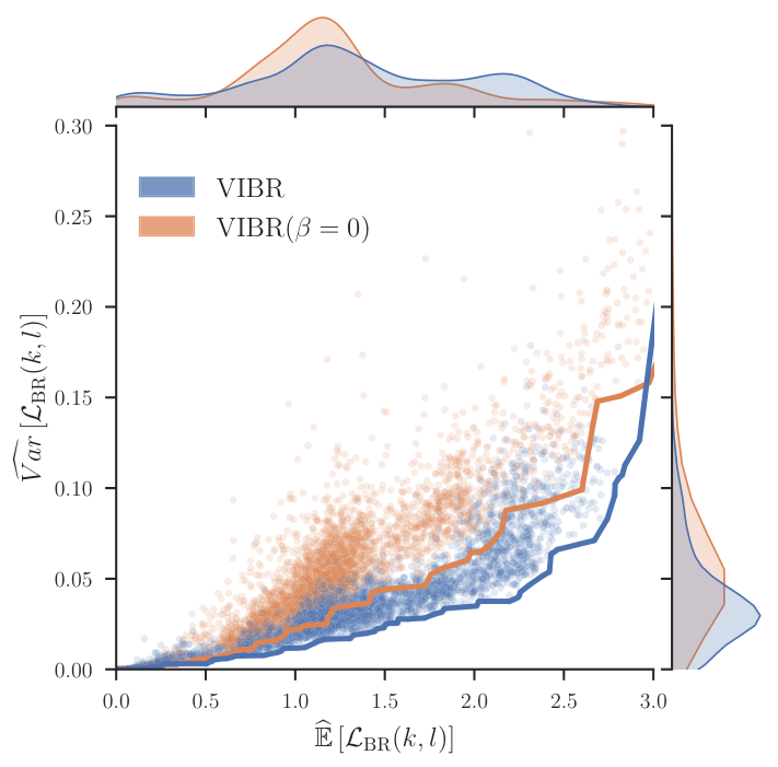
We first investigate how does the variance regularization term weighted by $\beta$ influences learning dynamics and help generalization. During training, we save the pair $\left(\widehat{\mathbb{E}}\left[\mathcal{L}_{\mathrm{BR}}(k,l)\right],\widehat{Var}\left[\mathcal{L}\mathrm{BR}(k,l)\right]\right)$ for every batch and plot them in Figure 5(b). We compare training with $\beta>0$ and $\beta=0$ on Walker Walk aggregated on 4 seeds. As visible by the lower Pareto frontier and the marginals, the regularizer has the intended effect described in section 3.2: a positive $\beta$ shifts the overall distribution towards lower $\widehat{Var}\left[\mathcal{L}\mathrm{BR}(k,l)\right]$ during training. Consequently, the marginal $\widehat{\mathbb{E}}\left[\mathcal{L}_{\mathrm{BR}}(k,l)\right]$ is more uniform and less concentrated around lower values when $\beta>O$ . This means that the model effectively perform a trade-off between bias on some of the views/observers in order to keep the variance low. When we plot the distribution of $\widehat{Var}\left[\mathcal{L}_{\mathrm{BR}}(k,l)\right]$ across time steps (Figure 5(c)), we notice that most of the regularization is impactful at the beginning of training but does not affect asymptotic convergence. This mechanism is particularly helpful as deep reinforcement learning networks are known to suffer from early overfitting preventing them from reaching higher performance in the long run (Nikishin et al. 2022). In our case, early overfitting happens on the training domain C0* which is indicated by excellent performance of all baselines on C0 even when generalization fails.

Additional Results

We study the $\beta$ hyperparamter by measuring IQM as a function of $\beta$ for all 6 environments of the DCS (Figure 6). Notably, all environments approximately converge to a zero variance of IQM between evaluation domains. We notice that difference in environment dynamics influence the choice for optimal $\beta$ . Note that we did not change the default action repeat hyperparameter of DCS. This makes Cartpole Swingup an extremely difficult task with an action repeat of 8 while having dynamic distractions in the background and explains the surprisingly low performance despite the simple mechanics. Further detailed results can be found in Appendix H and I, as well as an ablation study of the loss components in Appendix J showing the importance of using all pairwise bellman residuals in VIBR.

5 Related Works

Robust Visual RL

Although not studied in this work, data augmentation is an efficient and easy to implement method to regularize models and increase generalization performance. Some methods study which type of data augmentation is better suited for RL: random shifts (Yarats et al. 2020; Yarats et al. 2021; Laskin et al. 2020b), data mixing and convolutions (Wang et al. 2020; Zhang & Guo 2021; Zhou et al. 2020) or masking (Lee et al. 2020; Seo et al. 2023; Xiao et al. 2022). A more efficient method for robust RL is using domain randomization. Hansen & Wang 2021; Stone et al. 2021; Grigsby & Qi 2020 modify the original Deepmind Control Suite (Tassa et al. 2018) to include visual distractions, Xing et al. 2021; Zhu et al. 2020; Ahmed et al. 2020 involve robotic tasks and and causality. Akkaya et al. 2019 dynamically adapts domain randomization intensity and Ren et al. 2020 use an adversarial objective. Other works use parallel environments with different randomizations (Ren et al. 2020; Li et al. 2021; Zhao & Hospedales 2021; James et al. 2019; Zhang et al. 2020).

Invariant Representation Learning

is another approach to ensure good generalization across visual perturbations. Zhang et al. 2021a; Agarwal et al. 2021a; Bertran et al. 2022 uses behavioural metric learning. Other works relate invariant prediction (Peters et al. 2016; Arjovsky et al. 2019), robust optimization and causal inference to isolate causal feature sets and keep only task-relevant features , (Zhang et al. 2020; Sonar et al. 2021). Multiple work use the Block-MDP setting to learn invariant representations (Zhang et al. 2021b; Zhang et al. 2021a; Agarwal et al. 2021a; Bertran et al. 2022; Efroni et al. 2021). Other works focus on model learning: Lu et al. 2020 combines data augmentation with counterfactuals to learn a structured causal model with an adversarial objective, while Wang et al. 2022 learn noise-invariant world-models. Li et al. 2021 also uses an adversarial objective combined with gradient reversal to learn a representation robust to interventions. Mozifian et al. 2020 apply bisimulation and risk extrapolation (Krueger et al. 2021) on robotics. We differ from this line of work as VIBR does not need any auxiliary representation learning loss.

6 Discussion and conclusion

Our method has the obvious limitation of requiring multiple views during training. However, we emphasize that our multi-view assumption is only necessary during the learning phase and not at inference time. This becomes particularly advantageous in Sim2Real settings, where simulating multiple points of view is cost-effective, whereas providing multiple viewpoints at inference may be sometimes more challenging. Simulations can be used to intervene on the visual aspects of the environment without necessitating additional views for real-world inference.

However, as there is a limited number of simulated benchmarks specifically designed for multi-view training setups in image-based reinforcement learning, it is both plausible and practical to use multiple views at inference time in many real-life scenarios using multiple cameras. This is an affordable and prevalent practice in robotics platforms and autonomous vehicles, which often employ multiple sensors and cameras to address redundancies and potential occlusions.

While the baselines do not require this assumption, limiting the training setup to a single frame or view of the scene can therefore be unnecessarily restrictive and may not reflect actual practical use cases. The main objective of this paper is to serve as a proof-of-concept for the efficient utilization of existing multi-view training setups, such as those already found in the robotics domain.

Therefore, assuming multiple view availability, we presented VIBR (View-Invariant Bellman Residuals), a method that combines multi-view training and invariant prediction to reduce out-of-distribution (OOD) generalization gap for RL based visuomotor control. We demonstrated strong generalization results on the Distracting Control Suite benchmark and to our knowledge, VIBR is the first method to provide non-trivial performance on the hardest setting of DCS (C4). We also provided an analysis of the learning dynamics of VIBR which helped us explain its competitive performance compared to representation learning methods. Further work include finding appropriate architectures for multi-view training, scaling the model and data size to tackle more complex visuomotor control challenges, automatic tuning of $\beta$ with (meta-)learning or heuristics and leveraging pretrained generative models to sample observers without having access to a simulation or multiple cameras.

Acknowledgments

This publication was made possible by the use of the FactoryIA supercomputer, financially supported by the Ile-De-France Regional Council.

References

Agarwal et al. (2021a) Rishabh Agarwal, Marlos C Machado, Pablo Samuel Castro, and Marc G Bellemare. Contrastive behavioral similarity embeddings for generalization in reinforcement learning. In International Conference on Learning Representations, 2021a.
Agarwal et al. (2021b) Rishabh Agarwal, Max Schwarzer, Pablo Samuel Castro, Aaron C Courville, and Marc Bellemare. Deep reinforcement learning at the edge of the statistical precipice. Advances in Neural Information Processing Systems, 34, 2021b.
Ahmed et al. (2020) Ossama Ahmed, Frederik Träuble, Anirudh Goyal, Alexander Neitz, Manuel Wuthrich, Yoshua Bengio, Bernhard Schölkopf, and Stefan Bauer. Causalworld: A robotic manipulation benchmark for causal structure and transfer learning. In International Conference on Learning Representations, 2020.
Akkaya et al. (2019) Ilge Akkaya, Marcin Andrychowicz, Maciek Chociej, Mateusz Litwin, Bob McGrew, Arthur Petron, Alex Paino, Matthias Plappert, Glenn Powell, Raphael Ribas, et al. Solving rubik’s cube with a robot hand. arXiv preprint arXiv:1910.07113, 2019.
Arjovsky et al. (2019) Martin Arjovsky, Léon Bottou, Ishaan Gulrajani, and David Lopez-Paz. Invariant risk minimization. arXiv preprint arXiv:1907.02893, 2019.
Bardes et al. (2022) Adrien Bardes, Jean Ponce, and Yann Lecun. Vicreg: Variance-invariance-covariance regularization for self-supervised learning. In ICLR 2022-10th International Conference on Learning Representations, 2022.
Bellemare et al. (2019) Marc Bellemare, Will Dabney, Robert Dadashi, Adrien Ali Taiga, Pablo Samuel Castro, Nicolas Le Roux, Dale Schuurmans, Tor Lattimore, and Clare Lyle. A geometric perspective on optimal representations for reinforcement learning. Advances in neural information processing systems, 32, 2019.
Bertran et al. (2022) Martin Bertran, Walter Talbott, Nitish Srivastava, and Joshua Susskind. Efficient embedding of semantic similarity in control policies via entangled bisimulation. arXiv preprint arXiv:2201.12300, 2022.
Bradbury et al. (2018) James Bradbury, Roy Frostig, Peter Hawkins, Matthew James Johnson, Chris Leary, Dougal Maclaurin, George Necula, Adam Paszke, Jake VanderPlas, Skye Wanderman-Milne, and Qiao Zhang. JAX: composable transformations of Python+NumPy programs, 2018. URL http://github.com/google/jax.
Chen et al. (2020) Xinlei Chen, Haoqi Fan, Ross Girshick, and Kaiming He. Improved baselines with momentum contrastive learning. arXiv preprint arXiv:2003.04297, 2020.
Dabney et al. (2021) Will Dabney, André Barreto, Mark Rowland, Robert Dadashi, John Quan, Marc G Bellemare, and David Silver. The value-improvement path: Towards better representations for reinforcement learning. In Proceedings of the AAAI Conference on Artificial Intelligence, volume 35, pp. 7160–7168, 2021.
Du et al. (2019) Simon Du, Akshay Krishnamurthy, Nan Jiang, Alekh Agarwal, Miroslav Dudik, and John Langford. Provably efficient rl with rich observations via latent state decoding. In International Conference on Machine Learning, pp. 1665–1674. PMLR, 2019.
Efroni et al. (2021) Yonathan Efroni, Dipendra Misra, Akshay Krishnamurthy, Alekh Agarwal, and John Langford. Provably filtering exogenous distractors using multistep inverse dynamics. In International Conference on Learning Representations, 2021.
Grigsby & Qi (2020) Jake Grigsby and Yanjun Qi. Measuring visual generalization in continuous control from pixels. arXiv preprint arXiv:2010.06740, 2020.
Grill et al. (2020) Jean-Bastien Grill, Florian Strub, Florent Altché, Corentin Tallec, Pierre Richemond, Elena Buchatskaya, Carl Doersch, Bernardo Avila Pires, Zhaohan Guo, Mohammad Gheshlaghi Azar, et al. Bootstrap your own latent-a new approach to self-supervised learning. Advances in neural information processing systems, 33:21271–21284, 2020.
Haarnoja et al. (2018) Tuomas Haarnoja, Aurick Zhou, Pieter Abbeel, and Sergey Levine. Soft actor-critic: Off-policy maximum entropy deep reinforcement learning with a stochastic actor. In International conference on machine learning, pp. 1861–1870. PMLR, 2018.
Hansen & Wang (2021) Nicklas Hansen and Xiaolong Wang. Generalization in reinforcement learning by soft data augmentation. In 2021 IEEE International Conference on Robotics and Automation (ICRA), pp. 13611–13617. IEEE, 2021.
Hoffman et al. (2020) Matthew W. Hoffman, Bobak Shahriari, John Aslanides, Gabriel Barth-Maron, Nikola Momchev, Danila Sinopalnikov, Piotr Stańczyk, Sabela Ramos, Anton Raichuk, Damien Vincent, Léonard Hussenot, Robert Dadashi, Gabriel Dulac-Arnold, Manu Orsini, Alexis Jacq, Johan Ferret, Nino Vieillard, Seyed Kamyar Seyed Ghasemipour, Sertan Girgin, Olivier Pietquin, Feryal Behbahani, Tamara Norman, Abbas Abdolmaleki, Albin Cassirer, Fan Yang, Kate Baumli, Sarah Henderson, Abe Friesen, Ruba Haroun, Alex Novikov, Sergio Gómez Colmenarejo, Serkan Cabi, Caglar Gulcehre, Tom Le Paine, Srivatsan Srinivasan, Andrew Cowie, Ziyu Wang, Bilal Piot, and Nando de Freitas. Acme: A research framework for distributed reinforcement learning. arXiv preprint arXiv:2006.00979, 2020.
Jaderberg et al. (2017) Max Jaderberg, Volodymyr Mnih, Wojciech Marian Czarnecki, Tom Schaul, Joel Z Leibo, David Silver, and Koray Kavukcuoglu. Reinforcement learning with unsupervised auxiliary tasks. In International Conference on Learning Representations, 2017.
James et al. (2019) Stephen James, Paul Wohlhart, Mrinal Kalakrishnan, Dmitry Kalashnikov, Alex Irpan, Julian Ibarz, Sergey Levine, Raia Hadsell, and Konstantinos Bousmalis. Sim-to-real via sim-to-sim: Data-efficient robotic grasping via randomized-to-canonical adaptation networks. In Proceedings of the IEEE/CVF Conference on Computer Vision and Pattern Recognition, pp. 12627–12637, 2019.
Krueger et al. (2021) David Krueger, Ethan Caballero, Joern-Henrik Jacobsen, Amy Zhang, Jonathan Binas, Dinghuai Zhang, Remi Le Priol, and Aaron Courville. Out-of-distribution generalization via risk extrapolation (rex). In International Conference on Machine Learning, pp. 5815–5826. PMLR, 2021.
Laskin et al. (2020a) Michael Laskin, Aravind Srinivas, and Pieter Abbeel. Curl: Contrastive unsupervised representations for reinforcement learning. In International Conference on Machine Learning, pp. 5639–5650. PMLR, 2020a.
Laskin et al. (2020b) Misha Laskin, Kimin Lee, Adam Stooke, Lerrel Pinto, Pieter Abbeel, and Aravind Srinivas. Reinforcement learning with augmented data. Advances in neural information processing systems, 33:19884–19895, 2020b.
Lee et al. (2020) Kimin Lee, Kibok Lee, Jinwoo Shin, and Honglak Lee. Network randomization: A simple technique for generalization in deep reinforcement learning. In International Conference on Learning Representations, 2020.
Li et al. (2021) Bonnie Li, Vincent François-Lavet, Thang Doan, and Joelle Pineau. Domain adversarial reinforcement learning. arXiv preprint arXiv:2102.07097, 2021.
Lu et al. (2020) Chaochao Lu, Biwei Huang, Ke Wang, José Miguel Hernández-Lobato, Kun Zhang, and Bernhard Schölkopf. Sample-efficient reinforcement learning via counterfactual-based data augmentation. arXiv preprint arXiv:2012.09092, 2020.
Mozifian et al. (2020) Melissa Mozifian, Amy Zhang, Joelle Pineau, and David Meger. Intervention design for effective sim2real transfer. arXiv preprint arXiv:2012.02055, 2020.
Nikishin et al. (2022) Evgenii Nikishin, Max Schwarzer, Pierluca D’Oro, Pierre-Luc Bacon, and Aaron Courville. The primacy bias in deep reinforcement learning. In International Conference on Machine Learning, pp. 16828–16847. PMLR, 2022.
Peters et al. (2016) Jonas Peters, Peter Bühlmann, and Nicolai Meinshausen. Causal inference by using invariant prediction: identification and confidence intervals. Journal of the Royal Statistical Society: Series B (Statistical Methodology), 78(5):947–1012, 2016.
Rahaman et al. (2019) Nasim Rahaman, Aristide Baratin, Devansh Arpit, Felix Draxler, Min Lin, Fred Hamprecht, Yoshua Bengio, and Aaron Courville. On the spectral bias of neural networks. In International Conference on Machine Learning, pp. 5301–5310. PMLR, 2019.
Ren et al. (2020) Yangang Ren, Jingliang Duan, Shengbo Eben Li, Yang Guan, and Qi Sun. Improving generalization of reinforcement learning with minimax distributional soft actor-critic. In 2020 IEEE 23rd International Conference on Intelligent Transportation Systems (ITSC), pp. 1–6. IEEE, 2020.
Schwarzer et al. (2021) Max Schwarzer, Ankesh Anand, Rishab Goel, R Devon Hjelm, Aaron Courville, and Philip Bachman. Data-efficient reinforcement learning with self-predictive representations. In International Conference on Learning Representations, 2021.
Seo et al. (2023) Younggyo Seo, Danijar Hafner, Hao Liu, Fangchen Liu, Stephen James, Kimin Lee, and Pieter Abbeel. Masked world models for visual control. In Conference on Robot Learning, pp. 1332–1344. PMLR, 2023.
Sonar et al. (2021) Anoopkumar Sonar, Vincent Pacelli, and Anirudha Majumdar. Invariant policy optimization: Towards stronger generalization in reinforcement learning. In Learning for Dynamics and Control, pp. 21–33. PMLR, 2021.
Stone et al. (2021) Austin Stone, Oscar Ramirez, Kurt Konolige, and Rico Jonschkowski. The distracting control suite–a challenging benchmark for reinforcement learning from pixels. arXiv preprint arXiv:2101.02722, 2021.
Tassa et al. (2018) Yuval Tassa, Yotam Doron, Alistair Muldal, Tom Erez, Yazhe Li, Diego de Las Casas, David Budden, Abbas Abdolmaleki, Josh Merel, Andrew Lefrancq, et al. Deepmind control suite. arXiv preprint arXiv:1801.00690, 2018.
Wang et al. (2020) Kaixin Wang, Bingyi Kang, Jie Shao, and Jiashi Feng. Improving generalization in reinforcement learning with mixture regularization. Advances in Neural Information Processing Systems, 33:7968–7978, 2020.
Wang et al. (2022) Tongzhou Wang, Simon Du, Antonio Torralba, Phillip Isola, Amy Zhang, and Yuandong Tian. Denoised mdps: Learning world models better than the world itself. In International Conference on Machine Learning, pp. 22591–22612. PMLR, 2022.
Xiao et al. (2022) Tete Xiao, Ilija Radosavovic, Trevor Darrell, and Jitendra Malik. Masked visual pre-training for motor control. arXiv preprint arXiv:2203.06173, 2022.
Xing et al. (2021) Eliot Xing, Abhinav Gupta, Sam Powers, and Victoria Dean. Kitchenshift: Evaluating zero-shot generalization of imitation-based policy learning under domain shifts. In NeurIPS 2021 Workshop on Distribution Shifts: Connecting Methods and Applications, 2021.
Yarats et al. (2020) Denis Yarats, Ilya Kostrikov, and Rob Fergus. Image augmentation is all you need: Regularizing deep reinforcement learning from pixels. In International Conference on Learning Representations, 2020.
Yarats et al. (2021) Denis Yarats, Rob Fergus, Alessandro Lazaric, and Lerrel Pinto. Mastering visual continuous control: Improved data-augmented reinforcement learning. In International Conference on Learning Representations, 2021.
Zhang et al. (2020) Amy Zhang, Clare Lyle, Shagun Sodhani, Angelos Filos, Marta Kwiatkowska, Joelle Pineau, Yarin Gal, and Doina Precup. Invariant causal prediction for block mdps. In International Conference on Machine Learning, pp. 11214–11224. PMLR, 2020.
Zhang et al. (2021a) Amy Zhang, Rowan Thomas McAllister, Roberto Calandra, Yarin Gal, and Sergey Levine. Learning invariant representations for reinforcement learning without reconstruction. In International Conference on Learning Representations, 2021a.
Zhang et al. (2021b) Amy Zhang, Shagun Sodhani, Khimya Khetarpal, and Joelle Pineau. Learning robust state abstractions for hidden-parameter block mdps. In International Conference on Learning Representations, 2021b.
Zhang & Guo (2021) Hanping Zhang and Yuhong Guo. Generalization of reinforcement learning with policy-aware adversarial data augmentation. arXiv preprint arXiv:2106.15587, 2021.
Zhao & Hospedales (2021) Chenyang Zhao and Timothy Hospedales. Robust domain randomised reinforcement learning through peer-to-peer distillation. In Asian Conference on Machine Learning, pp. 1237–1252. PMLR, 2021.
Zhou et al. (2020) Kaiyang Zhou, Yongxin Yang, Yu Qiao, and Tao Xiang. Domain generalization with mixstyle. In International Conference on Learning Representations, 2020.
Zhu et al. (2020) Yuke Zhu, Josiah Wong, Ajay Mandlekar, and Roberto Martín-Martín. robosuite: A modular simulation framework and benchmark for robot learning. arXiv preprint arXiv:2009.12293, 2020.

Appendix A Impact of $\beta$ on VIBR gradient norm

We show here that a strictly positive $\beta$ value for the VIBR loss helps during training by preventing overfitting towards a deep single domain minimum and encouraging convergence to moderate local minima, thus helping extrapolation. Let $X=\mathcal{L}_{\mathrm{BR}}(k,l)$ . The gradients of VIBR loss can be written:

	$\displaystyle\nabla\mathcal{L}_{\mathrm{VIBR}}$	$\displaystyle=\hat{\mathbb{E}}\left[\nabla X\right]+\beta\nabla\hat{Var}(X)$
		$\displaystyle=\hat{\mathbb{E}}\left[\nabla X\right]+\beta\nabla\left(\hat{\mathbb{E}}\left[X^{2}\right]-\hat{\mathbb{E}}\left[X\right]^{2}\right)$
		$\displaystyle=\hat{\mathbb{E}}\left[\nabla X\right]+\beta\hat{\mathbb{E}}\left[2X\nabla X\right]-2\beta\hat{\mathbb{E}}\left[\nabla X\right]\hat{\mathbb{E}}\left[X\right]$
		$\displaystyle=\hat{\mathbb{E}}\left[\nabla X+2\beta\left(X\nabla X-\hat{\mathbb{E}}\left[X\right]\nabla X\right)\right]$
		$\displaystyle=\hat{\mathbb{E}}\left[\nabla X\left(1+2\beta\left(X-\hat{\mathbb{E}}\left[X\right]\right)\right)\right]$

This proves that gradients of VIBR are completely aligned with TD-learning gradient when looking at a sample in particular, but only change the norm of the gradient based on the sign of $\left(X-\hat{\mathbb{E}}\left[X\right]\right)$ . As a result, for a given $(k,l)$ pair of observers:

•

if $\mathcal{L}_{\mathrm{BR}}(k,l)<\hat{\mathbb{E}}\left[{L}_{\mathrm{BR}}\right]$ (overfitting to one observer pair $(x^{k},x^{l})$ , then the weight of this update is reduced

$\lVert\nabla\mathcal{L}_{\mathrm{VIBR}}(x^{k},x^{l})\rVert<\lVert\nabla{L}_{\mathrm{BR}}(k,l)\rVert$
•

if $\mathcal{L}_{\mathrm{BR}}(k,l)>\hat{\mathbb{E}}\left[{L}_{\mathrm{BR}}\right]$ (underfitting to one observer pair $(x^{k},x^{l})$ , then the weight of this update is increased

$\lVert\nabla\mathcal{L}_{\mathrm{VIBR}}(x^{k},x^{l})\rVert>\lVert\nabla{L}_{\mathrm{BR}}(k,l)\rVert$

This mechanism discourages overfitting to deep minimum and actively promotes converging towards ”hard-to-optimize” regions. An example of such region is a domain that is located very far from the overfitting domain: ensuring good performance on it would be difficult as shown in Figure 2(b). Because OOD domains minima are more likely to be located far from obvious minimum where overfitting is frequent, the variance regularization term encourages fitting to domains that might be closer to OOD, which helps generalization.

Appendix B $\beta$ Hyperparameter Study

Figure 6: Study of the impact of

\beta

on generalization and invariance. Shaded areas are bootstrapped CI.

Appendix C Continuous Control with VIBR

SAC

Soft Actor-Critic (Haarnoja et al. 2018) extends Q-learning to continuous control with an entropy maximizing actor-critic algorithm. The policy loss is defined as follow:

J_{\pi}(\phi)=\mathbb{E}_{\mathbf{s}_{t}\sim\mathcal{D}}\left[\mathbb{E}_{\mathbf{a}_{t}\sim\pi_{\phi}}\left[\alpha\log\left(\pi_{\phi}\left(\mathbf{a}_{t}\mid\mathbf{s}_{t}\right)\right)-Q_{\theta}\left(\mathbf{s}_{t},\mathbf{a}_{t}\right)\right]\right]=\mathbb{E}_{\mathbf{s}_{t}\sim\mathcal{D}}\left[L_{\pi}(\mathbf{s}_{t})\right]

As in DQN, the temporal-difference loss also minimizes Bellman residuals to learn the action-value function but with a different target: it has an additional entropy regularization term and sample the target action according to the soft-policy. $\mathbf{a}_{t+1}\sim\pi_{\phi}(\mathbf{s}_{t})$ :

Q_{\text{target}}=r_{t}+\gamma\left(Q_{\bar{\theta}}(\mathbf{s}_{t+1},\mathbf{a}_{t+1})-\alpha\log\pi_{\phi}\left(\mathbf{a}_{t+1}\mid\mathbf{s}_{+1}\right)\right)

where $\alpha$ is a temperature parameter controlling exploration and is either fixed or trainable.

DrQ

(Yarats et al. 2020) is an extension of SAC that largely improves visual RL performance on continuous control tasks. It achieves such results with random shift data augmentation, averaging the Q-target over $K$ image transformations and averaging the Q-function itself over $M$ image transformations.

Appendix D Representation Learning for RL

DBC

(Zhang et al. 2021a) learns invariant representations using bisimulation metrics. It learns to put 2 distincts embedding of states at a fixed pre-computed pseudo-distance depending on behavioral similarity and optimizes the following loss function for the encoder $\phi$ :

J(\phi)=\left(\left\|\mathbf{z}_{i}-\mathbf{z}_{j}\right\|_{1}-\left|r_{i}-r_{j}\right|-\gamma W_{2}\left(\hat{\mathcal{P}}\left(\cdot\mid\overline{\mathbf{z}}_{i},\mathbf{a}_{i}\right),\hat{\mathcal{P}}\left(\cdot\mid\overline{\mathbf{z}}_{j},\mathbf{a}_{j}\right)\right)\right)^{2}

(16)

where $\mathbf{z}_{i}=\phi\left(\mathbf{s}_{i}\right),\mathbf{z}_{j}=\phi\left(\mathbf{s}_{j}\right),r$ are rewards, $\overline{\mathbf{z}}$ denotes $\phi(\mathbf{s})$ with stop gradients, $W_{2}$ denotes the earth-mover or 2-Wasserstein distance (which has a closed form for Gaussian distributions), and $\hat{\mathcal{P}}$ is a dynamics model with Gaussian distribution output.

SPR

(Schwarzer et al. 2021) learn time predictive representations of images by predicting multiple latent vectors into the future with a siamese architecture inspired from Grill et al. 2020. This method has a projection network and a cosine similarity loss.

\mathcal{L}_{\theta}^{\mathrm{SPR}}\left(s_{t:t+K},a_{t:t+K}\right)=-\sum_{k=1}^{K}\left(\frac{\tilde{y}_{t+k}}{\left\|\tilde{y}_{t+k}\right\|_{2}}\right)^{\top}\left(\frac{\hat{y}_{t+k}}{\left\|\hat{y}_{t+k}\right\|_{2}}\right)

(17)

CURL

is a natural extension of Chen et al. 2020 to RL where the teacher-student architecture (with a projection network) match two different views of the same observation (originally with data augmentation) with a InfoNCE loss of the form:

\mathcal{L}_{\mathrm{CURL}}=\log\frac{\exp\left(q^{T}Wk_{+}\right)}{\exp\left(q^{T}Wk_{+}\right)+\sum_{i=0}^{K-1}\exp\left(q^{T}Wk_{i}\right)}

(18)

FM(Feature-Matching)

is a very simple representation learning baselines adapted to our case, where we directly match representations of two observations from the same state given by two observers $x^{k}$ and $x^{l}$ . The loss (MSE) directly optimizes the encoder without projection network.

\mathcal{L}_{\mathrm{FM}}=\lVert\phi(x^{k}(s))-\phi(x^{l}(s))\rVert^{2}

(19)

For fairness of comparison, all baselines have access to the same training data as VIBR, and might freely benefit from having multiple observers the same way as VIBR does. We maximize their performance by matching two views from different observers in each baseline’s respective loss using the two-branch teacher-student architecture.

Appendix E Loss Landscape Toy Experiment

We create the plots of Figure 2(b) by creating a pseudo loss landscape of a 2d neural network with the following bivariate function:

f(x,y,a,b,c,d)=\left(\frac{x-a}{c}\right)^{2}+\left(\frac{y-b}{c}\right)^{2}+d

(20)

We implement the four domains by plotting 4 variation of $f$ along the range of parameters with the following values for $a,b,c$ and $d$ :

•

Bottom-left $\mathcal{D}^{1}$ : $a=b=c=1\qquad d=0$
•

Bottom-right $\mathcal{D}^{2}$ : $a=2\qquad b=1\qquad c=0.75\qquad d=0.25$
•

Top-left $\mathcal{D}^{3}$ : $a=1\qquad b=2\qquad c=0.75\qquad d=0.25$
•

Top-right $\mathcal{D}^{4}$ : $a=2\qquad b=2\qquad c=0.5\qquad d=0.4$

This parameters allows us to control the width and depth of each valley, which helps us simulate different training landscapes with different optimization difficulties. We apply $\tanh$ before plotting for better visualization. The plot on the left is obtained by taking $\min_{\mathcal{D}^{i}}f(x,y,\mathcal{D}^{i})$ for all $x,y$ . This is a practical way of visualizing all 4 domains at the same time, but does not reflect a single optimization objective. The middle plot is obtained with: $\widehat{\mathbb{E}}_{\mathcal{D}^{i}}\left[f(x,y,\mathcal{D}^{i})\right]$ for all $x,y$ . This corresponds to ERM if we suppose that the cardinality of each domain is equal. Finally, we obtain the plot on the right with $\widehat{\mathbb{E}}_{\mathcal{D}^{i}}\left[f(x,y,\mathcal{D}^{i})\right]+\beta\widehat{Var}\left(f(x,y,\mathcal{D}^{i})\right)$ for all $x,y$ . This effectively corresponds to V-Rex in Krueger et al. 2021 and our variance regularization term of VIBR.

Appendix F Implementation Details

Each experience in the paper is run on 4 different seeds for reproducibility. We base our VIBR implementation of the SAC implementation in ACME²² 2 https://github.com/deepmind/acme (Hoffman et al. 2020) in Jax (Bradbury et al. 2018), but modify it to fit DrQ architecture. Both policy and Q-network are implemented with convolutional stack followed by a MLP. The policy and Q-network only share weights of the convolution stack to compute lower-dimensional visual features. The convolutional stack (or ”encoder) is composed of 4 convolutional layers with 32 filters and $3\times 3$ kernel sizes. Stride is 2 for the first convolutional layer then 1 for the rest. Outputs features are flattened and put through a linear layer to reach a final dimension of 50. Layer normalization and tanh activation is applied to the features before passing them to actor or critic’s MLP. Encoder layers are initialized with delta orthogonal initialization, while all linear layers used Lecun uniform initialization. All networks use ReLU activations units. Trainig is done with the Adam optimizer, and all hyperparameters used are described in table 1. We optimize $\beta$ with hyperparameter search over $\left[10^{-3},\cdots,50\right]$ and find a value that maximizes IQM and transfer for each environment. Values are listed in the hyperparameter table.

We use the github³³ 3 https://github.com/geyang/gym-distracting-control implementation of the Distracting Control suite and modify it to create our training and evaluation curriculum.

Table 1: Hyperparameters

Hyperparameter	Value
Replay buffer size	100000
Initial collection steps	25000
Optimizer	Adam
Actor learning rate	3e-4
Critic learning rate	3e-4
Weight decay	0
Initial temperature $\alpha$	0.1
Temperature learning rate	3e-4
Batch size	128
$\tau$ EMA	5e-3
Actor hidden layers	[512, 512]
Critic hidden layers	[512, 512]
Frame stacking	3
Action repeat	8 if Cartpole; 2 if Finger, Walker; 4 otherwise
VIBR variance penalty $\beta$	5 if Walker; 0.1 if Ball in Cup; 1 otherwise

Appendix G Distracting Control Suite

We use Distracting Control Suite (Stone et al. 2021) for our experiments. DCS is a variant of the Deepmind Control Suite where visual distractions are dynamically added to the rendered observations. The perturbations consists in the following non-exclusive dimension of variations:

•

color randomization of physical bodies
•

background randomization with a dataset of videos
•

random camera wobbling around a fixed point

Distractions are dynamic, temporally consistent and continuous. Colors of bodies are continuously changing at each time step. The background is displaying frame by frame a randomly selected video from the DAVIS dataset, which is played forward then backward to avoid discontinuities. The camera’s orientation is rotating with a random angle at each step while keeping the agent in the field of view. We define our curriculum as follows:

•

C0: No visual perturbation, original DM Control environment
•

C1: Dynamic background changes with a dataset of 2 videos and random body colorization with an intensity parameter $\alpha$ of 0.1
•

C2: Dynamic background changes with a dataset of 4 videos, random body colorization and random camera wobbling with an intensity parameter $\alpha$ of 0.1
•

C3: Dynamic background changes with a dataset of 8 videos, random body colorization and random camera wobbling with an intensity parameter $\alpha$ of 0.2
•

C4: Dynamic background changes with a dataset of 50 videos, random body colorization and random camera wobbling with an intensity parameter $\alpha$ of 0.3

Training and evaluation curriculums have the same definition, except that training domains use a separate video dataset than evaluation domains to properly evaluate generalization both in-distribution and out-of-distribution. All models are consistently trained with both C0 and either C1, C2 or C3. Main results are obtained with C0 and C2. This allows us to easily define 2 observers $x^{0}$ and $x^{2}$ where $x^{0}(\mathcal{S})\in C0$ and $x^{2}(\mathcal{S})\in C2$ . Using these two observers, we produce 2 different view each on its own domain at each time step. We provide image samples of each environment for each domain of the curriculum in Figure 7

Appendix H Sample efficiency curves

Figure 8: Evaluation sample efficiency curves on C0. Line IQM and shaded area bootstrapped CI.

Figure 9: Evaluation sample efficiency curves on C1. Line IQM and shaded area bootstrapped CI.

Figure 10: Evaluation sample efficiency curves on C2. Line IQM and shaded area bootstrapped CI.

Figure 11: Evaluation sample efficiency curves on C3. Line IQM and shaded area bootstrapped CI.

Figure 12: Evaluation sample efficiency curves on C4. Line IQM and shaded area bootstrapped CI.

Appendix I IQM and Generalization Gap per Environment per Benchmark

Figure 13: IQM per environment per evaluation domain compared to baselines. Trained on C2*. Vertical bars are bootstrapped CI.

Figure 14: Generalization Gap per environment per evaluation domain compared to baselines. Trained on C2*. Vertical bars are bootstrapped CI.

Figure 15: IQM per environment per evaluation domain while changing training domain. Vertical bars are bootstrapped CI.

Figure 16: Generalization Gap per environment per evaluation domain while changing training domain. Vertical bars are bootstrapped CI.

Appendix J Ablations

We perform ablations on the $\widehat{\mathbb{E}}\left[\mathcal{L}_{\mathrm{BR}}(k,l)\right]$ term from the VIBR loss and show that all Bellman residuals terms are necessary for good performance. To perform the ablation, we disabled risk extrapolation by fixing $\beta$ to 0. Training is done on the C2* on the Walker Walk environment for 4 seeds.

Figure 17: IQM and bootstrapped CI of ablations on C0

Figure 18: IQM and bootstrapped CI of ablations on C1

Figure 19: IQM and bootstrapped CI of ablations on C2

Figure 20: IQM and bootstrapped CI of ablations on C3

Figure 21: IQM and bootstrapped CI of ablations on C4