Non-equilibrium quantum probing through linear response
Abstract
The formalism of linear response theory can be extended to encompass physical situations where an open quantum system evolves toward a non-equilibrium steady-state. Here, we use the framework put forward by Konopik and Lutz [Phys. Rev. Research 1, 033156 (2019)] to go beyond unitary perturbations of the dynamics. Considering an open system comprised of two coupled quantum harmonic oscillators, we study the system’s response to unitary perturbations, affecting the Hamiltonian dynamics, as well as non-unitary perturbations, affecting the properties of the environment, e.g., its temperature and squeezing. We show that linear response, combined with a quantum probing approach, can effectively provide valuable quantitative information about the perturbation and characteristics of the environment, even in cases of non-unitary dynamics.
I Introduction
The study of non-equilibrium scenarios is key for the dynamics – and thermodynamics – of quantum systems de Vega and Alonso 2017; Binder et al. 2018. Although an overarching framework to consistently interpret the variety of non-equilibrium quantum phenomena is hitherto missing, some light has been shed towards understanding several aspects of this multifaceted problem. These theoretical studies come together with a strong interest in applications concerned with transport phenomena, e.g., in quantum technologies at the nanoscale Benenti et al. 2017.
Given a non-equilibrium setting, the standard approach follows classical statistical mechanics Marconi et al. 2008, where one applies small perturbations to the system of interest to gather information about the system itself: depending on the nature of the perturbation, one would be able to deduce relevant physical properties through, e.g., response and relaxation functions or generalized susceptibilities Kubo et al. 2012. This simple, yet insightful, idea is the essence of linear response theory; this being usually the first step in trying to harness the otherwise complex phenomenology of non-equilibrium systems. However, it is worth emphasising that, when extended to quantum systems, Kubo’s original formulation of linear response theory relies on two assumptions Kubo 1966; Kubo 1957: the system is isolated so that its dynamics are unitary; furthermore, it relaxes towards a thermal equilibrium state. These conditions are not always met in practice. On one hand, closed quantum systems are usually a crude approximation, as we should effectively include environmental effects in the form of dissipation and/or decoherence Breuer and Petruccione 2002; Rivas and Huelga 2012. On the other hand, there are cases in which the system relaxes towards a non-equilibrium steady-state (NESS). This class of states is obtained, for instance, when considering boundary-driven systems, i.e., systems that are dissipatively driven by coupling with two different baths at the two ends Landi et al. 2022. The physical properties of the system and its bath (e.g., temperature or chemical potential), as well the intra-system and system-bath coupling will ultimately influence the transport properties.
In this work, we aim to probe the non-equilibrium dynamics of a system through linear response theory. To this end, we extend the customary domain of application of linear response theory to include non-unitary perturbations to the system dynamics. Non-unitary perturbations have been considered in Ref. Mehboudi et al. 2019b, where a method was put forward for finding the linear response of the covariance matrix to a perturbation in the Gaussian channel describing its evolution. The perturbation could be either unitary or non-unitary. Here we proceed via a different method where we find the linear response of an observable of the system to a perturbation in the master equation describing its evolution. As a paradigmatic setting of boundary-driven systems, we consider a simple yet highly non-trivial example and address two coupled harmonic oscillators locally interacting with their own bath. The non-vanishing interaction between the two parties eventually leads the composite system to a NESS. Furthermore, we assume that the dynamics of such a system are described by a local master equation which does not include memory effects, i.e., we rely on a fully Markovian description of the evolution Breuer and Petruccione 2002. This scenario has been analysed in Ref. Konopik and Lutz 2019, where, inspired by considerations coming from classical statistical mechanics Agarwal 1972; Seifert and Speck 2010; Baiesi and Maes 2013, a framework for non-equilibrium quantum linear response has been put forth. However, consistently with the original spirit of the linear response approach, the interest is usually limited to unitary perturbations Konopik and Lutz 2019; Levy et al. 2021 — e.g., to the interaction Hamiltonian between the two subsystems Konopik and Lutz 2019.
Here we use one of the two oscillators to test the effects of the perturbations to the bath that is locally coupled to the other one. This configuration is fully in line with the quantum probing paradigm, where it is customary to use a small, simple, and controllable system interacting with a more complex environment to infer accurate information about environmental parameters (e.g., temperature or spectral properties) Smirne et al. 2013; Benedetti et al. 2018; Tamascelli et al. 2020; Hartmann and Strunz 2021. In turn, the problem that we address is closely connected with quantum estimation theory Paris 2009; Giovannetti et al. 2006; Polino et al. 2020; Sidhu and Kok 2020; Campbell et al. 2017, for which the ultimate goal is to find the optimal measurement scheme to gain precise information about a set of given parameters characterising the system and its dynamics Stace 2010; Correa et al. 2015; De Pasquale and Stace 2018; Mehboudi et al. 2019a; Mitchison et al. 2020. Interestingly, within the context of non-equilibrium open quantum systems described by Markovian dynamical maps, a close relationship between fluctuation-dissipation theorems Campisi et al. 2011 and quantum metrology has been established Mehboudi et al. 2018, though limited to the static case: such a connection allows for the description of the effect of a perturbation within the linear response regime.
We first investigate the case where the probe itself is in contact with a thermal bath; despite the thermal noise, we are able to detect the changes to the environment interacting with the main system, when a sudden quench is applied to its temperature. In line with the general aim of quantitatively assessing the effects of a sudden change of the macroscopic parameters characterising the dissipation, we also consider the case where the system interacts with a thermal squeezed bath, while we assume that the probe is perfectly isolated. We show that linear response extended to the case of non-unitary dynamics remains effective in providing key information on the perturbation affecting the system and, when paired with a quantum probing approach, offers a valuable quantitative tool for the characterisation of the features of an environment.
The remainder of the paper is organized as follows. In Sec. II we set out the theory of linear response of open quantum systems to small perturbations. We try to keep our formalism as general as possible, so that both unitary and non-unitary perturbations can be applied to the system dynamics. In Sec. III we describe our first system of interest: a pair of coupled quantum harmonic oscillators, each interacting with local thermal environments. Given the nature of the systems and states that we consider, we can solve the dynamics analytically using the formalism of Gaussian quantum mechanics without the need for numerical approximations. In Sec. III.1 we apply two simultaneous perturbations – one unitary and one non-unitary. We then focus on the special case of a perturbation of the bath temperature. In III.2 we show that the second oscillator can serve as a probe of the response to a perturbation on the first oscillator. In Sec. IV, we detach one of the two subsystems (which becomes our probe) from the corresponding local bath, while we let the other subsystem interact with a local squeezed thermal bath. We then study the response of the probe to perturbations on the parameter controlling the squeezing of the bath. In Sec. V, we present our conclusions, along with an outlook for future directions.
II Linear response in open quantum systems
In this Section, we will review the formalism of linear response for open quantum systems. In particular, we will explicitly show that the linear response of a generic observable to a perturbation can be written in terms of the steady-state of the system and the observable of interest, written in the Heisenberg picture, where the time-evolution is solely controlled by the unperturbed dynamics Konopik and Lutz 2019. Since our aim is to investigate how the system responds whenever we perturb either the unitary or the non-unitary part of the dynamics, we will write the relevant equations in a general form. Thus we will work at the level of superoperators, with the Liouvillian of the dynamics expressed as the sum of a unitary part and a dissipator in the standard Lindbladian form Breuer and Petruccione 2002; Lindblad 1976; Gorini et al. 1976; Gorini et al. 1978. The dynamics of the system are described by the Markovian master equation
| (1) |
where the Liouvillian can be expanded (to first order) as
| (2) |
where with the unperturbed Hamiltonian and the system’s dissipator. Also, is the time-dependent parameter controlling the perturbation. Following lines similar to those in Ref. Konopik and Lutz 2019, we assume that, for a fixed value of , the dynamics possess a stationary state , i.e., , that can be expressed as
| (3) |
where is the steady-state of the unperturbed dynamics 11 1 In the following we use what in Ref. Konopik and Lutz 2019 is defined as a class one quantum response function, involving only the stationary state of the unperturbed dynamics. It is interesting to note that, to this end it is sufficient to assume that there exists a stationary state of the unperturbed dynamics., and its linear (in ) correction due to the perturbation. It is worth emphasising that is not necessarily an equilibrium state. When that is the case and the perturbation is unitary, we recover the standard Kubo formalism of linear response Kubo 1957.
Moreover, in general, the state at some time can be expressed as
| (4) |
where has to be traceless in order for to be a physical state. By substituting Eq. (4) into Eq. (1) and integrating over time we arrive at the final result
| (5) |
to first order in Konopik and Lutz 2019; Zwanzig 2001. It follows that the linear response of a generic observable can be written as
| (6) |
where is the unperturbed expectation value and is the linear response function. Note that this response function can be expressed as
| (7) |
where is the dual of the generator of the unperturbed dynamics, and evolves according to the adjoint master equation 22 2 Here and in the remainder of the manuscript, unless otherwise specified, we will assume units such that and the Boltzmann constant .
| (8) |
that encompasses the dual dissipator Breuer and Petruccione 2002.
III System in contact with local thermal baths

First, let us consider a system of two coupled quantum harmonic oscillators, each interacting with a local thermal bath, as depicted in Fig. 1. The unperturbed Hamiltonian of this system reads
| (9) |
where is the frequency of the first harmonic oscillator and is that of the second, which is detuned by a quantity , i.e., . The interaction between the two oscillators, controlled by the coupling strength , is modelled so as to preserve the total number of excitations across the closed system.
The open dynamics of the unperturbed system are governed by the master equation
| (10) |
where each local dissipator reads ()
| (11) | ||||
Each , defined in terms of the local creation and annihilation operators and , is the sum of two terms: the first describes the incoherent loss of excitations, while the second describes incoherent pumping. Here, is the damping rate (assumed to be the same for both oscillators), while the mean number of excitations for the -th thermal bath at inverse temperature is .
Given that the Liouvillian of the unperturbed dynamics is quadratic in the creation and annihilation operators, we can employ the methods of Gaussian quantum mechanics to solve the dynamics exactly. This is a valid approach as far as we restrict our considerations to Gaussian states and, as we will do in the following, to perturbations that are also quadratic forms of the operators of the oscillators. Hence we only need to study the evolution of the first and second moments of the dimensionless position and momentum operators and . Given the vector of quadratures , and starting from Eq. (10), it is straightforward to check that the first moments are damped to zero Ferraro et al. 2005. Therefore, if we assume – without loss of generality – the first moments to be initially zero, the system dynamics will be solely determined by the second moments. This is a customary assumption, e.g., when one considers optomechanical set-ups, where the Gaussian modes always represent zero-mean fluctuations around some semi-classical steady-state Vitali et al. 2007; Paternostro et al. 2006.
The second moments are encoded in the covariance matrix (CM) , whose entries are defined as . The time-evolution is thus expressed in the Lyapunov form as , where and are the drift and diffusion matrices, respectively. While the former bears dependence upon both the unitary and the non-unitary (dissipative) part of the dynamics, the latter only depends on the non-unitary part, describing the effect of thermal noise due to the interaction between the system and the environment. In order to obtain the linear response of an observable of the system as given in Eq. (6), we need the steady-state of Eq. (10) and the Heisenberg-evolved observable . The steady-state is completely characterized by the solution to , which can be found to read as [cf. Appendix A for the details of the calculations]
| (12) |
where , and
| (13) |
with , and . While, in general, the coupling between the two oscillators results in a non-thermal steady-state, in the limit , we have , , and , thus recovering the case of two independent quantum harmonic oscillators, each relaxing towards the corresponding thermal state.
We start by considering the observable . The corresponding adjoint master equation [cf. Eq. (8)] leads to a set of coupled differential equations, whose solution gives us
| (14) |
The explicit forms of the functions , and are given in Appendix B.
III.1 Two perturbations: coupling strength and temperature
Given the unperturbed dynamics in Eq. (10), we investigate the response to two perturbations, and : the former is a sudden quench in the coupling strength between the two harmonic oscillators, while the latter is a quench in the number of excitations of the first bath. Note that the linear response to a Hamiltonian perturbation of the coupling strength has been thoroughly studied in Ref. Konopik and Lutz 2019. The perturbed master equation reads
| (15) |
We take , where is a beamsplitter-like Hamiltonian perturbation of the form Aspelmeyer et al. 2014
| (16) |
where , and is the Heaviside step function.
We obtain the linear response of observable due to to the Hamiltonian perturbation as
| (17) |
Since , we can use Eq. (III), and rewrite the expectation values in terms of entries of the steady-state CM from Eq. (12). We get
| (18) |
where we have introduced the kernel function
| (19) |
with and .
Consider now a quench in the temperature of the environment of the first oscillator through a perturbation in described by
| (20) | ||||
where , with . The corresponding linear response is
| (21) |
After some algebra, we find
| (22) |
with [cf. Appendix B]. Finally, the linear response to a combination of perturbations to both the coupling strength of the interaction and the temperature of the first oscillator’s bath is obtained by simply adding the two aforementioned contributions. Therefore, the linear response (of the energy of the first oscillator) to both perturbations is
| (23) |
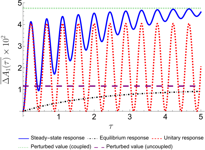
In Fig. 2, we show this response as a function of time for a certain choice of the parameters of the system (see caption) and with perturbation strengths and . We can also compare the linear response result with the exact dynamics of the perturbed system. In order to do so, we consider the steady-state reached asymptotically by the system when setting the coupling strength to and the average number of excitations in the bath of the first oscillator to , i.e., taking the perturbations into account. The difference between this new steady-state and the original unperturbed steady-state shall be referred to as the perturbed value of the energy response of the oscillator. We first calculate the expectation value of over the steady-state , i.e., , as we are looking for asymptotic conditions. The invariance of the steady-state under the dynamics allows us to remove the time dependence, thus leaving
| (24) |
where are the elements of the CM associated with . From this, we need to subtract the expectation value calculated over the unperturbed steady-state, for which , i.e., . Using the CM given in Eq. (12) we can find the explicit form of the perturbed value of the energy response of the first oscillator, and compare it with the long time limit of Eq. (23). It is straightforward to show that the two expressions coincide to first order in and , consistently with the linear response theory approximation. In Fig. 2, we clearly see that the perturbations cause oscillations in the steady-state response. The amplitude of such oscillations is damped over time, until the linear response converges to the perturbed value as .
We also consider the case of where the oscillators are uncoupled and only interact with their own local bath. As each oscillator is in its own equilibrium state just before they are perturbed, we refer to this as the equilibrium response. Additionally, the case in which the system evolves unitarily can be recovered from Eq. (23) by taking . As expected, in this limit, we obtain reversible dynamics, so that the linear response displays recurrences over time, which essentially follow the energy flowing back and forth from one oscillator to the other.
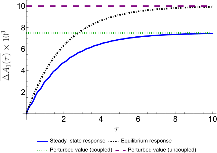
We now analyse a special case of the previous scenario, where we perturb only the temperature of the first bath, while we keep the coupling strength constant. Hence, the response is given by Eq. (22), or, equivalently, by setting in Eq. (23). The results are plotted in Fig. 3. In this case, where the perturbation affects only temperature, the linear response fully captures the exact dynamic response, which is calculated in Appendix. D. The equilibrium response here is identical to the equilibrium response in the case of two perturbations, consistently with the fact Eq. (18) vanishes for , reducing the case of two perturbations to just the response to the quench in temperature. In the equilibrium scenario, we have , thus Eq. (22) yields , which, as , converges to the asymptotic value . This is the maximum response possible, and it occurs when , i.e., when the oscillators are uncoupled. By contrast, whenever we switch on the coupling between the two oscillators, i.e., , the response of the first oscillator is comparatively smaller, as – through the interaction with the second oscillator – the first oscillator additionally experiences the effects of the second bath.
III.2 Second oscillator as a probe of a perturbation
Let us now consider the effect of a perturbation to the temperature of the first bath on the energy of the second oscillator. In order to do so, we apply a quench to the number of excitations in the first bath, and investigate the possibility of gaining information about this perturbation through the second oscillator, thus probing the environment of one subsystem through the response of the other. The linear response is once more given by Eq. (21) with replacing .
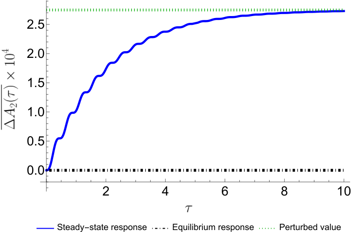


The response shown in Fig. 4 is qualitatively similar to that in Fig. 3, but the magnitude is smaller due to the fact that . Furthermore, the perturbation is now mediated by the first harmonic oscillator, which is the one whose bath is perturbed. As can be deduced from Fig. 4, whenever the coupling between the two oscillators is nonzero, the perturbation applied to the first oscillator affects the second one. As a result, the value of the coupling strength determines the response of the second oscillator. We provide evidence of this by exploring the limit , which corresponds to the equilibrium response. As we discussed in Sec. III, the equilibrium response of the first oscillator, shown in Fig. 3, approaches the maximum value , whilst the equilibrium response of second oscillator is zero [cf. Fig. 4]. For a finite value of the coupling constant , i.e., when we look at the steady-state response, the perturbation non-trivially affects the system response.
The difference between the perturbed value for coupled and uncoupled oscillators in Fig. 3 is related to the perturbed value of the second oscillator in Fig. 4 as
| (25) |
where is the perturbed value of the energy of the oscillator for a coupling strength . As , we find
| (26) |
This expression allows us to calculate the perturbed value of one of the oscillators if we know that of the other. This means that we can use the second oscillator as a probe to gain information about the response to a perturbation to the bath of the first. The degree to which the second oscillator mimics the first is determined by the coupling strength . We can add an additional line to the plots in Fig. 3 and Fig. 4 to show the behaviour as , illustrated in Fig. 5. Comparing Fig. 5 (a) and (b), we see that when , the energy response of the first oscillator approaches a value of , while – in the same limit – the response of the second oscillator tends towards . This shows that in the limit of infinite coupling strength, the energy of both oscillators increases by a factor proportional to . This can be interpreted as an instance of equipartition of energy between the two parties of the composite system.
IV System interacting with a single squeezed thermal bath

We now investigate a system comprised of two coupled quantum harmonic oscillators, one of which is connected to a squeezed thermal bath, as shown in Fig. 6. The environment is characterized by two parameters, i.e., its temperature and the squeezing parameter , which can be written in polar form as . The unitary dynamics of this system are described by the Hamiltonian given by Eq. (9). In this scenario, the unperturbed dynamics are governed by the following master equation Walls and Milburn 2008
| (27) |
where the dissipator – acting only on the first system – comprises the superoperators
| (28) | ||||
| (29) |
with , , and is the average number excitations in the bath at inverse temperature . The parameters and are not mutually independent as the condition must be enforced in order to ensure positivity of the density matrix Breuer and Petruccione 2002.
As in the case discussed in Sec. III, we need to find the steady-state or, equivalently, the corresponding CM. To do so, we follow a slightly different approach compared to that discussed in Sec. III. The core idea is to remap – resorting to a standard set of correspondence rules Gardiner and Zoller 2004 – the master equation from Eq. (27) into a Fokker-Planck equation for the characteristic function of our two-mode system, defined as
| (30) |
where is the displacement operator associated to the -th mode Walls and Milburn 2008; Cahill and Glauber 1969. The steady-state characteristic function is then found by imposing the condition . By inspection, from one can construct the steady-state CM, i.e., , written in terms of the annihilation and creation operators. In general, the entries of are defined as
| (31) |
with . Note that and are related by the transformation , where is defined as with
| (32) |
The details of the derivation of the steady-state CM are given in the Appendix C, whereas here we state the final result, i.e.,
| (33) |
where the explicit form of the coefficients , and is provided in Appendix C. These coefficients ultimately depend on the physical parameters characterising the dynamics of the system. In particular, in the limit , both and vanish, as one can immediately check through Eqs. (69) and (70). In other terms, when the two oscillators are uncoupled, the steady-state is given by a block-diagonal CM in the form
| (34) |
where the steady-state CM associated with the first mode, i.e.,
| (35) |
is non-diagonal due to the squeezing of the associated bath, whereas the second mode converges to the diagonal CM . Furthermore, in the limit , we have that the coefficient D vanishes and the system relaxes towards a global thermal state.

IV.1 Perturbation to bath squeezing
Given this system, we apply the linear response formalism outlined in Sec. II to study the effect of a perturbation to the squeezing of the first bath. More concretely, the perturbation is described by the superoperator
| (36) |
We restrict our attention to the case of a sudden perturbation, which we model through the step-like function (). The link between and entails that a step-like perturbation on the former will in turn cause a similar perturbation on the latter of the same form as from Eq. (20). The values of and are related as
| (37) |
under the assumption that the squeezing parameter is not directly affected by the perturbation. The linear response is obtained by accounting for both the perturbations in Eq. (20) and Eq. (36), i.e.
| (38) |
As we aim to use the second oscillator as a probe, we choose the observable to determine the linear response in dimensionless units. The calculation of the time-evolution of for this situation follows lines analogous to those previously illustrated, leading to
| (39) |
where , and are defined in Appendix B.
Plugging Eq. (39) into Eq. (38), we find that the contribution coming from is zero, hence the linear response reduces to
| (40) |
which is of the same form as that used in Sec. III, provided that the time-evolution of is obtained from Eq. (39), and the steady-state is deduced from the CM in Eq. (33). The linear response is finally given by
| (41) |
which is plotted in Fig. 7.
The perturbed value of the energy of the second oscillator is given by , where the change in is caused by the perturbation of the parameter . At long times, the measurement of the change in the energy of the second oscillator gives a value for . Hence we can deduce the change in squeezing, , of the bath attached to the first oscillator from Eq. (37). This shows that we can use the second oscillator as a probe of the perturbation to the squeezing of the bath interacting with the first oscillator.
V Conclusions and outlook
We have used the formalism of linear response theory to investigate both unitary and non-unitary perturbations around non-equilibrium steady-states of an open quantum system consisting of two coupled harmonic oscillators. We have calculated the response to simultaneous perturbations to the coupling strength between the two oscillators (i.e., a unitary perturbation), and to the temperature of the thermal bath (i.e., a non-unitary perturbation). We also looked at the effect solely determined by the temperature perturbation, investigating the response of both the oscillators to this. We found that such an approach is effective in probing perturbations to the dynamics of the system, including in situations where the latter is affected with a non-equilibrium bath.
The approach presented in this paper shows how to extend the theory of quantum linear response to non-unitary perturbations affecting the dynamics of open systems. Our study calls for a mathematically consistent formalism able to microscopically account for such perturbations. This would allow quantitative analysis of more general scenarios where the dynamical equations go beyond the usual Markovian approximation, encompassing, e.g., strong-coupling and memory effects.
Acknowledgements.
We acknowledge support from the European Union’s Horizon 2020 FET-Open project TEQ (766900), the Horizon Europe EIC Pathfinder project QuCoM (Grant Agreement No. 101046973), the Leverhulme Trust Research Project Grant UltraQuTe (grant RGP-2018-266), Deutsche Forschungsgemeinschaft (DFG, German Research Foundation) project number BR 5221/4-1, the Royal Society Wolfson Fellowship (RSWF/R3/183013), the UK EPSRC (EP/T028424/1), and the Department for the Economy Northern Ireland under the US-Ireland R&D Partnership Programme.Appendix A Steady-state covariance matrix for the first case
For the system described in Sec.III, we find the steady-state using the method set out in Appendix C of Ref. Mehboudi et al. 2019b to transform some classes of Lindbladian master equations into dynamical equations for the first and second moments. Let us consider a Lindbladian master equation in the form
| (42) |
where the Hamiltonian is quadratic in the quadrature operators, i.e., it can be written in the following matrix form
| (43) |
where is the vector of quadratures, while the Lindbladian operators are linear, i.e., . It is immediate to see that the master equation given by Eq. (10) fulfils these requirements, provided that we rewrite the relevant quantities in terms of the quadratures and , which are related to the set of creation and annihilation operators, and , by a linear transformation, as outlined in Sec. III. Therefore, the free Hamiltonian of Eq. (9) reads
| (44) |
The latter can be brought in the form of Eq. (43) by taking as vector of the quadratures, and
| (45) |
Comparing the unperturbed master equation in Eq. (11) with the general form in terms of the jump operators, i.e., Eq. (42), we can identify the jump operators as
| (46) |
Following Ref. Mehboudi et al. 2019b, we seek the vectors such that ; they are given by
| (47) |
The vectors allow us to construct the matrix
| (48) |
The drift matrix is obtained via Mehboudi et al. 2019b
| (49) |
where denotes the imaginary part of a matrix , and is the symplectic matrix given by , where
| (50) |
Substituting Eqs. (45) and (48) into Eq. (49) yields
| (51) |
The matrix is given by Mehboudi et al. 2019b
| (52) |
where Re() denotes the real part of a matrix . Substituting Eq. (48) into (52), the matrix turns out to be
| (53) |
Once the matrices and have been obtained, we can determine the steady-state CM, , by solving , which gives
| (54) |
where , , and . This matrix can be easily brought in the more compact form of Eq. (12).
Appendix B Time-evolution of observables
By following the derivation performed in Ref. Konopik and Lutz 2019, in this Appendix, we will explicitly show how to derive the time-evolution of the observable in the Heisenberg picture, under the dynamics of the first system with local thermal baths. As shown in Ref. Konopik and Lutz 2019, starting from the adjoint master equation in Eq. (8), we obtain a set of coupled differential equations, which can be recast in matrix form as
| (55) |
where
| (56) | ||||
| (57) |
and is the matrix
| (58) |
with and . For time-independent , integration yields
| (59) |
Taking the first entry of the vector v gives the time-evolution of as
| (60) |
where the functions in Eq. (60) are defined as
| (61) |
with
We use a very similar method to find the time-evolution of the observable for the second system, interacting with a squeezed bath, as detailed in Sec. IV. We find that
| (62) |
where the functions , and are defined as
| (63) | ||||
with , and .
Appendix C Steady-state covariance matrix for the second case
The dynamical system discussed in Sec. IV is governed by a master equation that does not resemble the general form given in Eq. (42). Therefore, we use a different method for finding the steady-state CM. As described in Ref. Walls and Milburn 2008, the master equation can be recast in the form of a Fokker-Planck (FP) equation for the two-mode characteristic function [cf. Eq. (30)] through the use of standard quantum optics correspondence relations. This allows us to write Eq. (27) as
| (64) |
with
| (65) | ||||
We consider the following ansatz for the form of the steady-state characteristic function
| (66) |
where we have introduced , the vector of first momenta of the steady-state, and the steady-state covariance matrix . By solving the algebraic equations stemming from enforcing the steady-state condition , we find
| (67) |
where
| (68) |
| (69) |
| (70) |
Appendix D Exact dynamic response
In the case of applying one perturbation to temperature or squeezing, the linear response, , is identical to the exact dynamic response, which we shall denote . We calculate the exact dynamic response in a similar way to the calculation for the perturbed value [cf. Eq. (24], but this time looking for the change in energy as a function of time rather than at the steady-state. For instance, to find the exact dynamic response of the energy of the first oscillator to a perturbation in temperature, we choose and calculate
| (71) |
In the expansion of given in Eq. (60), is the only term that depends on . Hence, Eq. (71) simplifies to
| (72) |
which exactly matches the linear response plotted in Fig. 3.
Similarly, for the perturbation in squeezing, note that is the only term that depends on the perturbed parameter, i.e., , in the expansion of our observed quantity [cf. Eq. (62)], which is in this case. Therefore, the exact dynamic response of the second oscillator to a perturbation in the squeezing of the first bath is given by . Again, the linear response perfectly reproduces this exact dynamic response.
References
- de Vega and Alonso (2017) I. de Vega and D. Alonso, Dynamics of non-markovian open quantum systems, Rev. Mod. Phys. 89, 015001 (2017).
- Binder et al. (2018) F. Binder, L. A. Correa, C. Gogolin, J. Anders, and G. Adesso, eds., Thermodynamics in the Quantum Regime, Fundamental Theories of Physics (Springer, Cham, 2018).
- Benenti et al. (2017) G. Benenti, G. Casati, K. Saito, and R. S. Whitney, Fundamental aspects of steady-state conversion of heat to work at the nanoscale, Physics Reports 694, 1 (2017).
- Marconi et al. (2008) U. M. B. Marconi, A. Puglisi, L. Rondoni, and A. Vulpiani, Fluctuation–dissipation: Response theory in statistical physics, Physics Reports 461, 111 (2008).
- Kubo et al. (2012) R. Kubo, M. Toda, and N. Hashitsume, Statistical physics II: Nonequilibrium Statistical Mechanics, Vol. 31 (Springer Berlin, Heidelberg, 2012).
- Kubo (1966) R. Kubo, The fluctuation-dissipation theorem, Reports on Progress in Physics 29, 255 (1966).
- Kubo (1957) R. Kubo, Statistical-mechanical theory of irreversible processes. i. general theory and simple applications to magnetic and conduction problems, J. Phys. Soc. Jpn. 12, 570 (1957).
- Breuer and Petruccione (2002) H.-P. Breuer and F. Petruccione, The Theory of Open Quantum Systems (Oxford University Press, Oxford, 2002).
- Rivas and Huelga (2012) A. Rivas and S. F. Huelga, Open Quantum Systems: An Introduction, SpringerBriefs in Physics (Springer-Verlag Berlin Heidelberg, 2012).
- Landi et al. (2022) G. T. Landi, D. Poletti, and G. Schaller, Nonequilibrium boundary-driven quantum systems: Models, methods, and properties, Rev. Mod. Phys. 94, 045006 (2022).
- Mehboudi et al. (2019b) M. Mehboudi, J. M. R. Parrondo, and A. Acín, Linear response theory for quantum gaussian processes, New Journal of Physics 21, 083036 (2019b).
- Konopik and Lutz (2019) M. Konopik and E. Lutz, Quantum response theory for nonequilibrium steady states, Phys. Rev. Res. 1, 033156 (2019).
- Agarwal (1972) G. S. Agarwal, Fluctuation-dissipation theorems for systems in non-thermal equilibrium and applications, Zeitschrift für Physik A 252, 25 (1972).
- Seifert and Speck (2010) U. Seifert and T. Speck, Fluctuation-dissipation theorem in nonequilibrium steady states, Europhysics Letters 89, 10007 (2010).
- Baiesi and Maes (2013) M. Baiesi and C. Maes, An update on the nonequilibrium linear response, New Journal of Physics 15, 013004 (2013).
- Levy et al. (2021) A. Levy, E. Rabani, and D. T. Limmer, Response theory for nonequilibrium steady states of open quantum systems, Phys. Rev. Res. 3, 023252 (2021).
- Smirne et al. (2013) A. Smirne, S. Cialdi, G. Anelli, M. G. A. Paris, and B. Vacchini, Quantum probes to experimentally assess correlations in a composite system, Phys. Rev. A 88, 012108 (2013).
- Benedetti et al. (2018) C. Benedetti, F. Salari Sehdaran, M. H. Zandi, and M. G. A. Paris, Quantum probes for the cutoff frequency of ohmic environments, Phys. Rev. A 97, 012126 (2018).
- Tamascelli et al. (2020) D. Tamascelli, C. Benedetti, H.-P. Breuer, and M. G. A. Paris, Quantum probing beyond pure dephasing, New Journal of Physics 22, 083027 (2020).
- Hartmann and Strunz (2021) R. Hartmann and W. T. Strunz, Open quantum system response from the hierarchy of pure states, The Journal of Physical Chemistry A 125, 7066 (2021).
- Paris (2009) M. G. A. Paris, Quantum estimation for quantum technology, International Journal of Quantum Information 07, 125 (2009).
- Giovannetti et al. (2006) V. Giovannetti, S. Lloyd, and L. Maccone, Quantum metrology, Phys. Rev. Lett. 96, 010401 (2006).
- Polino et al. (2020) E. Polino, M. Valeri, N. Spagnolo, and F. Sciarrino, Photonic quantum metrology, AVS Quantum Science 2, 10.1116/5.0007577 (2020).
- Sidhu and Kok (2020) J. S. Sidhu and P. Kok, Geometric perspective on quantum parameter estimation, AVS Quantum Science 2, 10.1116/1.5119961 (2020).
- Campbell et al. (2017) S. Campbell, M. Mehboudi, G. De Chiara, and M. Paternostro, Global and local thermometry schemes in coupled quantum systems, New J. Phys. 19, 103003 (2017).
- Stace (2010) T. M. Stace, Quantum limits of thermometry, Phys. Rev. A 82, 011611(R) (2010).
- Correa et al. (2015) L. A. Correa, M. Mehboudi, G. Adesso, and A. Sanpera, Individual quantum probes for optimal thermometry, Phys. Rev. Lett. 114, 220405 (2015).
- De Pasquale and Stace (2018) A. De Pasquale and T. M. Stace, Thermodynamics in the Quantum Regime., edited by F. Binder, L. Correa, C. Gogolin, J. Anders, and G. Adesso, Fundamental Theories of Physics, Vol. 195 (Springer, 2018) Chap. Quantum Thermometry.
- Mehboudi et al. (2019a) M. Mehboudi, A. Sanpera, and L. A. Correa, Thermometry in the quantum regime: recent theoretical progress, Journal of Physics A: Mathematical and Theoretical 52, 303001 (2019a).
- Mitchison et al. (2020) M. T. Mitchison, T. Fogarty, G. Guarnieri, S. Campbell, T. Busch, and J. Goold, In situ thermometry of a cold fermi gas via dephasing impurities, Phys. Rev. Lett. 125, 080402 (2020).
- Campisi et al. (2011) M. Campisi, P. Hänggi, and P. Talkner, Colloquium: Quantum fluctuation relations: Foundations and applications, Rev. Mod. Phys. 83, 771 (2011).
- Mehboudi et al. (2018) M. Mehboudi, A. Sanpera, and J. M. R. Parrondo, Fluctuation-dissipation theorem for non-equilibrium quantum systems, Quantum 2, 66 (2018).
- Lindblad (1976) G. Lindblad, On the generators of quantum dynamical semigroups, Communications in Mathematical Physics 48, 119 (1976).
- Gorini et al. (1976) V. Gorini, A. Kossakowski, and E. C. G. Sudarshan, Completely positive dynamical semigroups of -level systems, Journal of Mathematical Physics 17, 821 (1976).
- Gorini et al. (1978) V. Gorini, A. Frigerio, M. Verri, A. Kossakowski, and E. Sudarshan, Properties of quantum markovian master equations, Reports on Mathematical Physics 13, 149 (1978).
- (36) In the following we use what in Ref. Konopik and Lutz 2019 is defined as a class one quantum response function, involving only the stationary state of the unperturbed dynamics. It is interesting to note that, to this end it is sufficient to assume that there exists a stationary state of the unperturbed dynamics.
- Zwanzig (2001) R. Zwanzig, Nonequilibrium statistical mechanics (Oxford University Press, New York, 2001).
- (38) Here and in the remainder of the manuscript, unless otherwise specified, we will assume units such that and the Boltzmann constant .
- Ferraro et al. (2005) A. Ferraro, S. Olivares, and M. G. Paris, Gaussian States in Quantum Information (Bibliopolis, Naples, 2005).
- Vitali et al. (2007) D. Vitali, S. Gigan, A. Ferreira, H. R. Böhm, P. Tombesi, A. Guerreiro, V. Vedral, A. Zeilinger, and M. Aspelmeyer, Optomechanical entanglement between a movable mirror and a cavity field, Phys. Rev. Lett. 98, 030405 (2007).
- Paternostro et al. (2006) M. Paternostro, S. Gigan, M. S. Kim, F. Blaser, B. H. R, and M. Aspelmeyer, Reconstructing the dynamics of a movable mirror in a detuned optical cavity, New J. Phys. 8, 107 (2006).
- Aspelmeyer et al. (2014) M. Aspelmeyer, T. J. Kippenberg, and F. Marquardt, Cavity optomechanics, Rev. Mod. Phys. 86, 1391 (2014).
- Walls and Milburn (2008) D. Walls and G. Milburn, Quantum optics, 2nd ed. (Springer-Verlag Berlin Heidelberg, 2008).
- Gardiner and Zoller (2004) C. Gardiner and P. Zoller, Quantum Noise, 3rd ed., Springer Series in Synergetics (Springer-Verlag Berlin Heidelberg, 2004).
- Cahill and Glauber (1969) K. E. Cahill and R. J. Glauber, Ordered expansions in boson amplitude operators, Phys. Rev. 177, 1857 (1969).