Differentially Private Wireless Federated Learning Using Orthogonal Sequences
Abstract
We propose a privacy-preserving uplink over-the-air computation (AirComp) method, termed FLORAS, for single-input single-output (SISO) wireless federated learning (FL) systems. From the perspective of communication designs, FLORAS eliminates the requirement of channel state information at the transmitters (CSIT) by leveraging the properties of orthogonal sequences. From the privacy perspective, we prove that FLORAS offers both item-level and client-level differential privacy (DP) guarantees. Moreover, by properly adjusting the system parameters, FLORAS can flexibly achieve different DP levels at no additional cost. A new FL convergence bound is derived which, combined with the privacy guarantees, allows for a smooth tradeoff between the achieved convergence rate and differential privacy levels. Experimental results demonstrate the advantages of FLORAS compared with the baseline AirComp method, and validate that the analytical results can guide the design of privacy-preserving FL with different tradeoff requirements on the model convergence and privacy levels.
Index Terms:
Federated Learning; Differential Privacy; Orthogonal Sequences; Convergence Analysis.I Introduction
Real-world data generated or collected by edge devices enables various machine learning (ML) applications. For certain privacy-sensitive tasks, users prefer to keep their data locally instead of uploading to cloud servers. Federated learning (FL) [2, 3] has emerged as a distributed learning paradigm that caters to this growing trend, and is able to train a global ML model across all local datasets without the server having direct access to client data.
The local training nature of FL leads to massive communication costs, as an FL task consists of multiple learning rounds, each of which requires uplink and downlink model exchange between clients and the server. Compared with downlink broadcasting, uplink communication is more challenging in FL when communication is over the wireless medium [4, 5, 6]. Due to the stringent power constraints at mobile devices, channel noise and fading have a more conspicuous impact on uplink communications. More importantly, significant scalability challenges arise from the large number of clients in FL versus limited uplink communication resources. Uplink communication is known to be one of the key bottlenecks of wireless federated learning [2].
To tackle the scalability problem, over-the-air computation (also known as AirComp) mechanisms have been proposed. Instead of decoding individual local models of clients and then aggregating, AirComp allows multiple clients to transmit uplink signals in a naturally superpositioned fashion over a wireless medium, and decodes the average global model directly at the FL server. AirComp dramatically improves the scalability of wireless FL, and reduces the signal processing latency. Therefore, AirComp is regarded as a key technology for FL in wireless networks and has been investigated extensively [7, 8, 9, 10].
The most popular AirComp method is based on channel inversion power control [7], which “inverts” the fading channel at each transmitter so that the aggregated model can be directly obtained at the server. Variants and enhancements of AirComp have been studied, and a literature review can be found in Section II-A. Yet, a fundamental limitation of the existing methods is that they mostly require channel state information at the transmitter (CSIT). Enabling CSIT in wireless communication systems is complicated and is substantially harder than obtaining the channel state information at the receiver (CSIR). Moreover, channel inversion based on CSIT is well known to “blow up” when one of the users’ channels is in deep fade [11]. Hence, exploring CSIT-free AirComp methods becomes attractive[12].
Meanwhile, amidst a growing focus on data security, the importance of safeguarding individuals’ personal information has become increasingly emphasized. Although FL intuitively helps protect client privacy by keeping training data locally and never sharing it with the server, private information can still be leaked to some extent by analyzing the ML model parameters trained and uploaded by the clients [13, 14, 15]. To address the privacy concern, a natural way is to add (artificial) noise to ML model parameters in the upload phase of FL, whose privacy properties can be mathematically characterized using differential privacy (DP) [16].
AirComp has the potential to provide DP guarantee at no extra cost due to the inherent natural noise in the wireless channel. Heuristically, different DP levels can be guaranteed by controlling the signal-to-noise ratio (SNR), and thus the effective channel noise level, at the receiver side. Yet, most of the literature on AirComp rarely characterizes the achievable privacy in a mathematically rigorous fashion. A literature review can be found in Section II-B. Moreover, we note that the existing literature focuses only on item-level DP in wireless FL, while client-level DP (also known as user-level DP) [17] is a new metric that is particularly worth investigating for FL, which is largely missing.
To simultaneously remove the CSIT requirement of AirComp and address the privacy challenge, we propose FLORAS – Federated Learning using ORthogonAl Sequences, a novel uplink wireless physical layer design for FL by leveraging the properties of orthogonal sequences. On the communication design, FLORAS preserves all the advantages of AirComp while removing the CSIT requirement. From the perspective of privacy, FLORAS achieves desired DP guarantees (both item-level and client-level) by adjusting the number of used orthogonal sequences, making it much simpler and providing more flexibility to trade off privacy and utility.
The main contributions of this paper are summarized as follows:
- •
We propose FLORAS for uplink communications in single-input single-output (SISO) wireless FL systems. FLORAS enjoys all the advantages of AirComp, yet without the CSIT requirement. In particular, orthogonal sequences allow the base station (BS) to obtain individual CSIR via a single pilot, by which global ML model parameters can be estimated via simple linear projections. Therefore, FLORAS significantly reduces the channel estimation overhead. Different from the channel inversion power control, FLORAS allows the transmit power to be independent of the channel realizations, which avoids increasing the dynamic range of the transmit signal and improves the power efficiency.
- •
By adjusting the number of orthogonal sequences in the system configuration, the novel signal processing technique in FLORAS produces Cauchy effective noise to the decoded global model, which empowers flexible item-level and client-level DP guarantees. Moreover, a new FL convergence bound based on the truncated Cauchy noise is derived, which allows us to characterize the tradeoff between the model convergence rate and the achievable DP levels.
- •
We conduct extensive experiments based on real-world datasets to evaluate the performance of FLORAS. Numerical results demonstrate the performance advantages of FLORAS compared with the channel inversion method and validate our theoretical analysis by achieving tradeoffs between model convergence and DP.
The remainder of this paper is organized as follows. Literature review is presented in Section II. Section III introduces the FL pipeline and the uplink communication model. The proposed FLORAS design is detailed in Section IV. The DP guarantee and convergence analysis of FLORAS are presented in Section V and Section VI, respectively. Experimental results are reported in Section VII, followed by the conclusion of our work in Section VIII.
II Related Work
II-A AirComp for FL
The AirComp approach [7, 8, 9, 10] exploits the inherent signal superposition characteristics of a wireless multiple access channel to efficiently perform sum/average computations. This methodology can be considered as a special instance of computation over multiple access channels, as outlined by [18]. The approach has garnered significant attention due to its ability to minimize uplink communication costs, irrespective of the number of participating clients in FL. The exploration of client scheduling, along with various power and computation resource allocation techniques, has been investigated by [19, 20, 21, 22, 23]. Several studies have provided convergence guarantees for AirComp under diverse practical constraints and types of heterogeneity [24, 25, 26, 27, 28]. Efforts also have been made to reduce the CSIT requirement of AirComp. [29] relaxes full CSIT by utilizing only the phase information of the channel. Notably, [30] and [4] present CSIT-free AirComp methods that leverage channel orthogonality, although their effectiveness is limited to massive MIMO systems.
II-B Differential Privacy for FL
DP-SGD has been widely regarded as a standard approach to train a differentially private ML model [31]. Along with its variants[32, 33], recent years have also witnessed increased efforts on DP for distributed learning systems, including the clipping technique in [34, 35], the subsampling principle in [36], and random quantization in [37]. In the category of exploiting the channel noise for differentially private FL, [38] proposes an AirComp design to achieve DP by adjusting the effective noise; [39, 40] investigate adding noise and power allocation in non-orthogonal multiple access (NOMA) systems; [41] considers DP amplification via user sampling and wireless aggregation; [42] applies it to personalized FL. [43] jointly optimizes the latency and DP requirements of FL, and [44] discusses the tradeoff among privacy, utility, and communication.
III System Model
III-A FL Model
Consider an FL task with a parameter server and clients. Each client stores a (disjoint) local dataset , with its size denoted by . The amount of the total data is . We use to denote the local loss function at client , which measures how well an ML model with parameter fits its local dataset. The global objective function over all clients can be expressed as
where is the weight for each local loss function, and the goal of FL is to find the optimal model parameter that minimizes the global loss function:
We define to capture the degree of the non-independent and identically distribution (non-IID) of local datasets [45], where and are the minima of global and local loss functions, respectively.
The FedAvg framework [2] keeps client data locally, and the global model is obtained at the parameter server by the composition of multiple learning rounds. One of the key characteristics of FL is partial clients participation, i.e., only a portion of clients are selected in a single learning round for model upload. Here, we assume that of total clients are uniformly randomly selected during each learning round for the FL task. To simplify the notation, we use the subscript to indicate the participating clients during a given learning round, acknowledging that they could correspond to different clients in different rounds.
A typical wireless FL pipeline iteratively executes the following steps in the -th learning round.
- 1.
Downlink wireless communication. The BS broadcasts the current global model to all selected devices over the downlink wireless channel.
- 2.
Local computation. Each client uses its local data to train a local ML model improved upon the received global model . We assume that mini-batch stochastic gradient descent (SGD) is adopted to minimize the local loss function. The parameter is updated iteratively (for steps) at client as:
where denotes the stochastic gradient at client on model and mini-batch .
- 3.
Uplink wireless communication. Each involved client uploads its latest local model to the server synchronously over the uplink wireless channel.
- 4.
Server aggregation. The BS aggregates the received noisy local models to generate a new global model. For simplicity, we assume that each local dataset has an equal size, i.e., ; therefore we have .
This work focuses on steps and in the FL pipeline. In particular, we leverage the unique properties of orthogonal sequences, which leads to an efficient FL uplink communication design with DP guarantees.
III-B Communication Model
In each learning round, since there are active clients, the uplink communication between clients (mobile devices) and the parameter server (base station) can be modeled as over a fading multiple access channel. Consider a cell with a single-antenna BS and single-antenna users involved in one round of the aforementioned FL task. The communication system leverages orthogonal sequences for uplink transmissions. Note that one of the most popular implementations of the orthogonal sequence-based system is code-division multiple access (CDMA). We assume a spreading sequence set containing unique spreading sequences (), where each spreading sequence is denoted as and is the length of the spreading sequence. Each user is (randomly) assigned with a unique spreading sequence from as its signature.
We assume that the BS only has knowledge of the entire spreading sequence set , without knowing the specific signature of each user. We emphasize that this restriction is consistent with our goal of guaranteeing user privacy – BS cannot identify users or decode individual models based on their spreading sequences. We will discuss the details of the spreading sequence assignment mechanism in Section V-D.
In the uplink communication, each client transmits the differential between the received global model and the computed new local model:
The BS aims at estimating .
Before the transmission of , client will apply a normalization technique. We denote
as the normalized transmit signal. The following normalization technique, adopted in [7], ensures and :
where is the sample mean of elements in . Note that normalization parameters , and will be determined by the BS and clients via a separate control channel as suggested in [7]. The -norm bound guaranteed in the normalization not only provides the sensitivity of for the DP analysis in Section V, but also satisfies the practical requirement that each client has a limited transmit power. We note that the similar technique has also been applied in [34].
To simplify the notation, we omit index and use instead of barring any confusion. We assume that each client transmits every element of the model differential via shared time slots. In addition, block fading channel is assumed11 1 The large-scale pathloss and shadowing effect is assumed to be taken care of by, e.g., open loop power control [46], which is a common practice in real-world systems., i.e., the fading channel between each client and the BS remains unchanged in time slots. We emphasize that we do not make any specific assumption on the fading distribution throughout this paper. In the -th slot, each client transmits symbol spread by its uniquely assigned orthogonal sequence . The BS received signal can be written as
where is the additive white Gaussian noise (AWGN) with mean zero and variance per dimension. Note that since the model differential parameters are real signals, we only need to consider the real parts of channel coefficients and noise. Although one-dimensional (real) modulation cannot fully leverage the channel degrees of freedom, it is consistent with the fact that binary phase-shift keying (BPSK) is the most common modulation scheme in CDMA systems [11]. In addition, focusing on the real dimension makes the subsequent discussion easier and highlights our contribution better. Also, as we detail later in Remark 2, we can leverage full channel gain at an affordable cost of partial CSIT.
We note that spreading sequences are orthonormal, i.e.,
| (1) |
At the BS, the receiver will decode the estimated aggregation parameter , which is a noisy version of , and recover in slots. After that, the BS can perform de-normalization:
and compute the new global model as
| (2) |
Throughout the paper, we assume that all users are synchronized in frames, which can be achieved by the BS sending a beacon signal to initialize uplink transmissions [46].
IV FLORAS
We present the FLORAS design for uplink communications in wireless FL, and give some preliminary analysis.
IV-A Algorithm Design
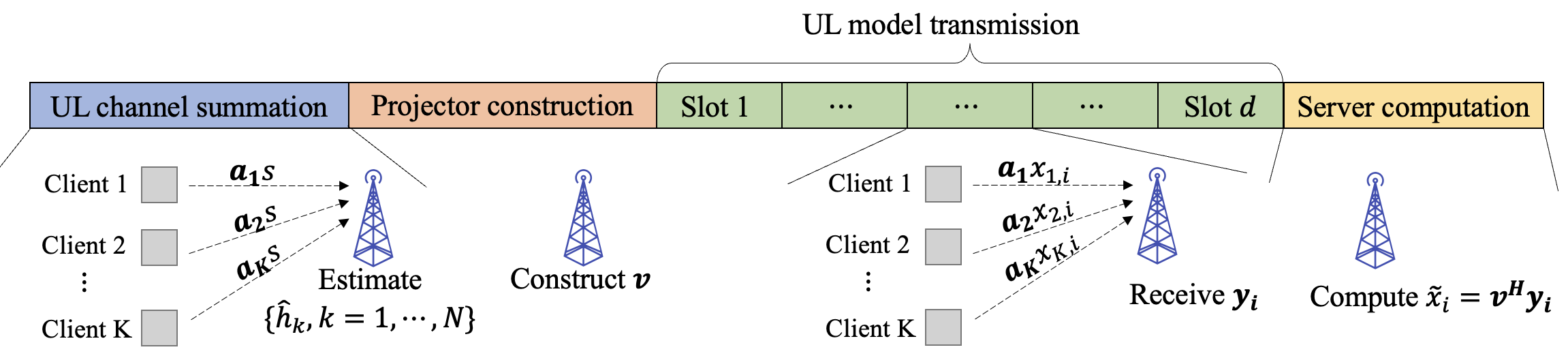
FLORAS is a four-step protocol detailed as follows.
Step 1: Uplink channel estimation. The BS first schedules all participating users to transmit a common pilot simultaneously. The received signal is
The BS can utilize and the complete set of orthogonal sequences to estimate the channel gain coefficients. For the spreading sequences that are actually adopted by the user22 2 Without loss of generality, we assume the first spreading sequences from the set are selected. This assumption is made to ease the notation., we have
For the spreading sequences that are not selected by any user, the BS obtains
We emphasize that the BS is not able to distinguish these two cases; all it has are estimates .
Step 2: Projector construction. For simplicity, we assume in the following discussion. After the channel estimation, the BS constructs the following vector based on all of the estimated channel coefficients:
We note that since the BS does not know which of the total spreading sequences are adopted by the users, it has to use all of to construct the projector . This seemingly redundant design actually enables better privacy protection, which will be clear in Section V.
Step 3: UL model transmission. All users transmit every element of the differentials via shared time slots:
IV-B Preliminary Analysis
In the high signal-to-noise ratio (SNR) regime, where the channel fading effect dominates the noise, we have . Therefore, we can establish the following approximation for the estimated model in Step :
| (3) |
where denotes the dominant noise of the received global model parameters33 3 Note that this approximation drops the minor noise term, which results in that the DP guarantee in the later discussion is a lower bound of the true DP level of FLORAS, i.e., we achieve better DP than that computed in this paper.. The distribution of this post-processing noise is not straightforward, and we next present Lemma 1 to establish that the noise term is a Cauchy random variable.
Lemma 1.
Define . For IID Gaussian random vector , random variable
with probability density function (PDF)
Proof.
We first note that and are Gaussian random variables since they are linear combinations of IID Gaussian random variables. Let
and
and it is straightforward to verify that and are IID Gaussian random vectors with distribution , where is a covariance matrix. According to [47], we have
as long as is independent of and . Letting and using the fact that if , we prove Lemma 1. ∎
Cauchy distribution is known as a “fat tail” distribution, as the tail of its PDF decreases proportionally with . Lemma 1 suggests that, for a fixed , a larger spreading sequence set will result in a heavier tail in the Cauchy noise. Therefore, we can adjust the size of the spreading sequence set to induce different additive Cauchy noise in (3). We will discuss the effect of Cauchy noise on DP and convergence in Sections V and VI, respectively.
A few remarks about FLORAS are now in order.
Remark 1 (Advantages over the channel inversion method).
Compared with the widely studied channel inversion-based AirComp design, FLORAS does not require CSIT for uplink communications, which greatly reduces the communication overhead. This is especially attractive for Internet-of-Things (IoT) applications with massive devices. Moreover, in SISO systems, the maximum uplink transmit power of each user in the channel inversion-based methods is usually limited by the worst channel gain. As a result, the received SNR of the global model and the efficiency of power amplifiers (PAs) will significantly decrease, if one of the client channels experiences deep fading [11]. Thanks to the orthogonality of spreading sequences, FLORAS allows the transmit power to be independent of small-scale fading channel realizations, and thus avoids increasing the dynamic range of the transmit signal, which improves the power efficiency of PAs.
Remark 2 (Leverage full channel degrees of freedom).
As mentioned before, real modulation cannot exploit full degrees of freedom of the complex channel. To address this limitation, we can borrow the idea of [29]. Specifically, the fading channel between each client and the BS can be written as
where and represent channel amplitude (gain) and phase, respectively. For a given , client transmits symbol , where is the phase correction term as suggested in [29]. Hence the received signal at the BS can be written as
By phase correction, the imaginary part of is projected to the real domain and the full channel gain can be leveraged without sacrificing any other advantages of FLORAS. We note that same as in [29], this approach requires each client to have the channel phase information , which is weaker than the complete CSIT but stronger than the standard FLORAS.
Note that we consider the imperfect channel estimation previously in Step for uplink communication. For simplicity, we assume that each client has perfect partial CSIT (channel phases) obtained from downlink channel estimation here. One reason for this different consideration is that the transmit power at the BS is usually much larger than those at devices, which naturally ensures more accurate downlink channel estimation than uplink. Additionally, even if the phase correction term suffers from estimation error, as long as the error is within , the proposed design is still valid [29], only at a cost of some channel gain lost.
Remark 3 (Extensions on NOMA systems).
Another limitation of FLORAS is that the number of orthogonal spreading sequences is fixed for a given sequence length. To expand the size of set , the system would need to adopt longer spreading sequences, which consumes more bandwidth. We first note that although there may exist a large number of clients in an FL task, the number of actively participating clients in each learning round is usually relatively small (due to client selection), which implies the bandwidth cost will not be too significant for our design. Second, as an alternative, the system can adopt non-orthogonal spreading sequences to improve the scalability without the cost of extra bandwidth. Applying non-orthogonal spreading sequences is consistent with non-orthogonal multiple access (NOMA) systems, which is an emerging technology for massive machine-type communications (mMTC) applications. For non-orthogonal spreading sequences, the requirement in (1) becomes
which can be achieved by random Gaussian vectors. Note that Lemma 1 still holds for non-orthogonal spreading sequences, since it allows an arbitrary covariance matrix of random Gaussian vectors and . Non-orthogonal spreading sequences will introduce inter-symbol interference besides noise when decoding the global model parameters in Step . Therefore, the convergence bound developed in Section VI can be regarded as a lower bound for NOMA systems.
V Differential Privacy Analysis
In this section, we analyze the DP level achieved by FLORAS. We begin by introducing the basic concepts of DP in FL, and then prove that FLORAS achieves different levels of DP via the adjustment of the size of spreading sequence set and the number of involved clients . Both item-level and client-level DP are analyzed. The DP guarantee not only considers multiple sources of randomness in wireless FL, including random mini-batch in SGD, the Cauchy noise, and the random client participation, but also reveals the influence of multiple learning rounds.
V-A Preliminaries
We first introduce the concept of neighboring datasets. We say that two datasets and are neighboring, written as , if they differ in at most one sample. Based on this concept, we state the standard definition of -DP as follows.
Definition 1 (-DP [16]).
A randomized algorithm provides -DP with , if for all pairs of neighboring datasets and all measurable sets of outcomes , we have
We say that a randomized algorithm achieves -DP (also known as pure DP) if it satisfies -DP with . The common interpretation of is the “leakage probability”, i.e., -DP is -DP “except with probability ”.
We next introduce the definition of Rényi DP [48]. As a generalization of -DP, it can help us obtain a tighter -DP bound converted from its composition, which is particularly attractive in FL due to its multiple learning rounds.
Definition 2 (-Rényi DP [48]).
A randomized algorithm is said to provide -Rényi DP, if for any pair of neighboring datasets it holds that
where
is the Rényi divergence. Specially, for , we have
In the AirComp FL design, decoding the global model from the received signal can be regarded as a randomized mechanism on , where is the union of the local datasets of all clients throughout the whole FL task. We denote this randomized mechanism as
| (4) |
where is the noise-free summation of model differentials at the -th learning round, and is a random noise following a certain distribution. The randomness of the mechanism comes from the random client participation, random mini-batch SGD, and the random noise.
To determine the DP level, we next define the global sensitivity function for the operator as
| (5) |
where is a neighboring dataset of . As mentioned in Section III, for uplink communications, we ensure that . Therefore, we have
| (6) |
where denotes the noise-free model differential from client whose local dataset is swapped in a random data sample.
V-B Item-level Differential Privacy
The Rényi DP guarantee of FLORAS in a single learning round is given in Theorem 1.
Theorem 1.
Assume a spreading sequence set containing unique sequences and total clients involved in an FL task. In each learning round, clients are independently and uniformly randomly selected to participate in FL. With local dataset of size and mini-batch size , FLORAS provides -Rényi DP for the global model, where
| (7) |
with , , and .
Proof.
See Appendix A-B. ∎
Based on the composition rule of Rényi DP, we next establish the -DP guarantee for the overall uplink communications in an FL task of rounds.
Theorem 2.
Consider a wireless FL task with learning rounds, a spreading sequence set containing unique sequences, and clients are independently and uniformly randomly selected in each round. With local dataset of size and mini-batch size , FLORAS provides -DP for the entire FL task, where
| (8) |
with , , and .
Proof.
See Appendix A-C. ∎
Theorems 1 and 2 reveal that, for a given FL configuration, i.e., fixed number of selected clients , mini-batch size ratio , participation ratio , and the number of learning rounds , the expansion of spreading sequence set would achieve a higher level of DP per learning round and for the whole learning task, respectively. In particular, in Rényi DP for each learning round, and in -DP for the whole learning task. Since the BS (adversary) has no knowledge of which particular out of the total spreading sequences the clients have chosen, increasing the number of spreading sequences results in a heavier tail of the post-processing Cauchy noise, which achieves better privacy protection.
Guided by Theorem 2, we can adjust to meet the privacy requirement of a practical FL task. Note that larger noise (better privacy protection) will affect the convergence rate of FL, and we will discuss this impact in detail in Section VI.
Remark 4 (Choice of DP metrics).
Note that we use -DP to evaluate the overall DP guarantee of the FL task. The reason why we choose to utilize Rényi DP to analyze the DP guarantee per learning round is the same as [49]: we can obtain a tighter -DP guarantee from the composition of multiple Rényi-DP mechanisms. This advantage is empirically shown in Fig. 2, in which we compare the overall DP guarantees v.s. learning rounds of three different composition methods: i) vanilla sequential composition of -DP; ii) advanced composition of -DP; iii) -DP converted from composition of Rényi DP. It clearly demonstrates that under different system configurations, Theorem 2 unanimously provides the tightest -DP guarantee, which is consistent with the theoretical and experimental results in [48].
V-C Client-level Differential Privacy
So far, we have focused on the standard item-level DP that protects a single data sample of a certain local dataset. For FL, another DP concept called client-level DP (also known as user-level DP) is also important. The definition of client-level DP follows similarly from Definition 1, with a slight change that the neighboring dataset pair differs in at most all data samples of one single client. As a result, client-level DP protects privacy when the entire data from a certain client is swapped. Intuitively, this guarantees that the participation of a client cannot be inferred by observing the received signals.
From the previous discussion of global sensitivity, the output is always bounded even though the entire dataset of a certain client changes. Therefore, our method intuitively satisfies the client-level DP, and we formally establish the following guarantee.
Theorem 3.
Given a spreading sequence set containing unique sequences, FLORAS provides -client level Rényi DP, when clients are independently and uniformly randomly selected from the total clients in each learning round, where
| (9) |
Moreover, for total learning rounds, FLORAS provides -client level DP for the entire FL task, where
| (10) |
Proof.
See Appendix A-D. ∎
Theorem 3 demonstrates that FLORAS provides the client-level DP guarantee in a manner that is similar to the item-level DP. However, since the entire local dataset of a certain client would be swapped, we cannot take advantage of the SGD randomness in the analysis of client-level DP. Therefore, disappears from the client-level DP guarantee.
V-D Spreading Sequence Assignment Mechanism
As we have discussed, the DP guarantee of FLORAS comes from the fact that the assignment of spreading sequences remains unknown to the BS (adversary). In traditional CDMA systems, the spreading sequence is assigned to each device by the BS. This mechanism becomes invalid in our setting, since we need to make sure that the BS only has knowledge of the spreading sequence set , not the individual assignment. In practice, we can resort to a trusted third-party to handle the assignment of orthogonal sequences. The design of such a mechanism belongs to the field of secure multi-party computation (MPC) [50, 51] and is out of the scope of this paper.
In the following, we provide a preliminary reference design based on a random permutation algorithm as illustrated in Fig. 3. The proposed design allows each user to autonomously choose a unique spreading code without collision. To better explain the mechanism, we first define a fixed matrix based on We assume that every device that will be involved in the FL task shares a common confidential Key. This key is a priori knowledge to clients, yet confidential to the BS (adversary). This assumption can be achieved via standard cryptography approaches, e.g., the key-exchange protocol [52]. When the BS schedules clients to participate in the current learning round, an index will be assigned to each client. After that, every client leverages the confidential Key and the current system time SystemTime() to generate a random seed RandSeed(). Since the system has been synchronized, each client will obtain the same random seed, and generate a (common) random permutation matrix based on that. Followed by a random column permutation each client can use the index-th column [:,index] as its spreading sequence for the current learning round. Note that as long as the confidential key is not leaked, the BS (adversary) will not know which of the total spreading sequences are adopted in the current learning round.
Remark 5.
We emphasize that the established DP guarantee is for the receiver processing proposed in Section IV-A. There may exist more sophisticated receiver algorithms, which could conceivably attempt to infer more information about the usage of the orthogonal sequences per learning round from the received signal. However, since we do not make any assumptions on the channel distribution, such approach would be difficult in general. Besides, it is impossible to always accurately identify all used sequences due to the channel noise. Therefore, even under this scenario, the proposed framework still provides privacy, although the DP guarantee dependency may decrease from to , where .

VI Convergence analysis
We analyze the ML model convergence behavior of FLORAS in this section. We first make the following standard assumptions that are commonly adopted in the convergence analysis of FedAvg and its variants; see [45, 53, 54, 5].
Assumption 1.
-smooth: and , ;
Assumption 2.
-strongly convex: and , ;
Assumption 3.
Unbiased SGD: , ;
Assumption 4.
Uniformly bounded gradient: , for all mini-batch data.
The main challenge, and hence the novelty of our analysis, lies in the Cauchy distributed post-processing noise. We note that a Cauchy distribution has uncertain (infinity) variance. To address this issue, the BS applies a truncation operation in the interval on the decoded global parameters in (3), before de-normalization:
| (11) |
where and is a normalization parameter defined in Section III-B. Note that the truncation operation is universal (albeit sometimes implicit) in almost all practical systems, since the signal values in the processing units are always finite. As a post-processing procedure, the truncation operation has no impact on the DP guarantee of FLORAS. Unfortunately, it will introduce a bias in the estimate , which impacts convergence. In particular, the equivalent noise after the limiting operation will be a truncated Cauchy distribution with support . Fortunately, as long as we ensure which requires a very mild truncation and thus is easy to satisfy, this operation will only have very limited impact on the received signal, hence does not significantly harm the convergence performance. We also note that biased gradients are very common in various DP-guaranteed SGD methods [32, 55, 56]. Moreover, after de-normalization, the biased term is effectively diminishing. Therefore, as we show in Theorem 4, FLORAS can still maintain a good convergence performance despite of the biased noise, which will also be numerically corroborated in Section VII.
Theorem 4.
With Assumptions 1-4 and , for some , if we set the learning rate as , a wireless system implementing FLORAS achieves
for any , where ,
and
Proof.
See Appendix B. ∎
Theorem 4 demonstrates that FLORAS preserves the convergence rate of SGD for strongly convex loss functions (compared with the noise-free FL convergence). For a fixed initial point, there are multiple factors in the constant that affect the convergence rate of FL. In particular, reveals the variance reduction effect of SGD by involving more clients, and and capture the influence of non-IID dataset and the number of local epochs, respectively. We note that term in demonstrates the impact from Cauchy noise, i.e. level of privacy protection. We also note that is increasing as becomes larger. It implies that a higher level of privacy protection will decrease the speed of convergence as constant becomes larger. Therefore, Theorem 4 establishes a tradeoff between privacy protection and convergence rate, which can guide the practical system design.
VII Experiments
In this section, we evaluate the performance of FLORAS through numerical experiments. We first compare the learning performance of FLORAS with the widely-investigated channel inversion AirComp method. Then, we evaluate the effect on the ML model convergence rate of various DP levels. In particular, we corroborate the theoretical results via real-world FL tasks on the MNIST dataset. The experiments demonstrate that FLORAS achieves superior performances under various SNRs and other system configurations.
Details on the setup of experiments are as follows. All convergence curves are the average of five independent Monte Carlo trials. The MNIST dataset contains multiple handwritten digit figures of pixels. The training set contains examples and is evenly distributed over clients. For the IID case, the data is shuffled and randomly assigned to each client; for the non-IID case, the data is sorted by labels and each client is randomly assigned with the data of one label. The test set size is . We evaluate FLORAS and validate the theoretical results on a multinomial logistic regression task. Specifically, let denote the prediction model with the parameter and the form . The loss function is given by . We adopt the regularization parameter in the experiments.
VII-A Communication Efficiency
We first evaluate the performance of FLORAS compared with the channel inversion method. We assume IID Raleigh block fading channel . For channel inversion, we adopt a user admission threshold for the fading channel gain to avoid deep fading. The following parameters are used for training: local batch size , the number of local epochs , and learning rate and for the IID and non-IID case, respectively.
Fig. 4-(a) and Fig. 4-(b) illustrate the training loss and test accuracy performance versus learning round of FLORAS and channel inversion in high (red line) and low (blue) SNR regimes, respectively. For high SNR ( dB), FLORAS and channel inversion have similar performances. Although transmitter fading channel cancellation in channel inversion limits the maximum transmission power of each user, its performance does not deteriorate, since noise is not the dominant factor of the convergence. However, we note that, unlike FLORAS, channel inversion requires full CSIT at each client, which not only consumes larger communication overhead, but also increases the dynamic range of the signal, bringing higher hardware cost. The advantages of FLORAS become conspicuous in the low SNR regime ( dB), in which noise becomes the dominant factor of the convergence rate. FLORAS allows all participated clients to make full use of transmit power and achieves significantly better performance. As shown in Fig. 4-(b), FLORAS achieves about higher test accuracy compared with channel inversion at SNR = dB. This phenomenon becomes more notable in the non-IID dataset as shown in Fig. 4-(c) and Fig. 4-(d), where the performance gap of test accuracy between FLORAS and channel inversion further grows to .
VII-B Differential Privacy
We also evaluate the convergence performance versus different levels of DP. We keep SNR dB and number of selected user , while changing the size of the orthogonal sequence set from to , i.e., and . In each learning round, each user selects its own signature from set via the method in Section V-D. As discussed in Section V, the larger size of set , the higher DP level FLORAS achieves. The following parameters are used for training: local batch size , the number of local epochs , and learning rate and for IID and non-IID cases, respectively. The training losses with different DP levels are illustrated in Fig. 5-(a) and Fig. 5-(c) of IID and non-IID cases, respectively. It is clear that although a higher privacy level decreases the convergence rate, the machine learning model can still converge with almost the same training loss as the no-differential-privacy case (), which is consistent with the theoretical analysis in Section VI. The test accuracies in Fig. 5-(b) and Fig. 5-(d) further validate the effectiveness of FLORAS. We can see that the test accuracies for moderate DP levels ( and ) are almost the same as the case of , i.e., we can achieve certain DP levels almost for free. Even when , the test accuracy loss is tiny, with about and compared with the case in the IID and non-IID datasets, respectively.
VIII Conclusion
We have proposed FLORAS, a differentially private AirComp FL framework. Compared with the channel inversion method, FLORAS does not require CSIT and has much more robust performance in the low SNR regime, which is crucial for IoT applications. The flexibility of adjusting the size of the orthogonal sequence set allows us to control both item-level and client-level DP guarantees of the system. From the analyses of convergence and DP of FLORAS, we have established the tradeoff between convergence rate and privacy preservation, which has been further validated by experiments on real-world FL tasks.
Appendix A Proofs of Theorems 1, 2, and 3
A-A Lemmas
We first establish the necessary lemmas for the proofs.
Lemma 2.
Let and be two Cauchy probability distributions and , with PDF and , respectively. reaches its maximum at with , and its minimum at with .
Proof.
The results can be directly obtained by taking the first-order derivative of and setting . ∎
Lemma 3 (Proposition in [57]).
Let and be probability distributions satisfying and . Then for all .
Lemma 4 (Proposition in [48]).
If is an -Rényi DP mechanism, it also satisfies -DP for any .
A-B Proof of Theorem 1
Define neighboring datasets and , where has one more element than . As we have assumed that all datasets have the same size , the size of is . We have and different mini-batches for dataset and , respectively. We further denote set as a collection of all the mini-batches corresponding to . We next calculate the number of mini-batches in dataset . It is straightforward to verify that , which reveals that there are mini-batches in that are the same as those in , and the remaining mini-batches are the ones that contain the data sample . We denote as a collection of all the mini-batches that contain the data sample . Therefore, all the possible mini-batches of are in .
We note that, in each learning round, of total clients are randomly selected. Therefore, there are total combinations of mini-batches in . We denote as the index set for the selected clients at -th learning round, and it is easy to verify that we have combinations for client selection per learning round. Therefore, we further denote each possible mini-batch combination as where . As for , there are total mini-batch combinations. Besides the same combinations in , there are additional mini-batch combinations in , which contains the mini-batch of the -th client and is chosen from . We denote them similarly as , where , and . In addition, we use to denote the noise-free global models calculated from mini-batch combination .
Building on these, the mechanism can be viewed as a random vector sampling from the following distribution:
Similarly,
| (12) |
We notice that and . Defining and , can be re-written as
where the first equality comes from replicating each of the items in the second summation in Eqn. (12) times, thus allowing the summation to be over the same range as the first summation.
A-C Proof of Theorem 2
A-D Proof of Theorem 3
Define neighboring datasets and , where is an arbitrary local dataset of a client . For dataset , of the total clients are randomly scheduled for the task in each learning round. We denote , where , as the set of all the possible client combinations during a single learning round for dataset . For dataset , beside the previous combinations, there are additional combinations that contain client . We denote them as . Therefore, the mechanism samples from the following distribution
Similarly,
By the definition of and following the similar techniques in Appendix A-B, and can both be bounded by . Again, based on Lemma 3, we can guarantee , which completes the single round DP guarantee. The proof of the client-level DP guarantee for the composition of rounds follows the same as that in Appendix A-C.
Appendix B Proof of Theorem 4
With a slight abuse of notation, we change the timeline to be with respect to the overall SGD iteration time steps instead of the communication rounds, i.e.,
Note that the global model is only accessible at the clients for specific , where , i.e., the time steps for communication. The notations for are similarly adjusted to this extended timeline, but their values remain constant within the same round. The key technique in the proof is the perturbed iterate framework in [59]. In particular, we first define the following variables for client :
where is the effective noise vector after de-normalization. Note that is a truncated Cauchy distribution vector with the following PDF:
where , . We further have
Then, we construct the following virtual sequences:
We also define and for convenience. Therefore, and . Note that the global model is only meaningful when . Hence, we have . Thus it is sufficient to analyze the convergence of to evaluate FLORAS.
B-A Lemmas
Lemma 5.
Let Assumptions 1-4 hold, is non-increasing, and for all . If , we have
Lemma 5 establishes a bound for the one-step SGD. This result only concerns the local model update and is not impacted by the noisy communication. The derivation is similar to the technique in [54] and is omitted.
Lemma 6.
Let Assumptions 1-4 hold. With for all and , we have
Proof.
Let denote the set of chosen indexes. Note that the number of possible is and we denote the th possible result as , where . Therefore,
Since when ,
for all , we have
Then
As for the variance, we have [45]
| (13) |
where we use the following results:
and
for all , and
Since , we know that is the communication time, implying that are identical. Then
Taking expectation over the randomness of stochastic gradient on Eqn. (13), we have
where in the last line is because is non-increasing and . ∎
Lemma 6 demonstrates a bound for the uniformly random selection. This result bounded the extra “noise” brought by partial participation. We note that in the full participation case, where . We note that the derivation of the proof is similar to the technique in [54].
Lemma 7.
Let Assumptions 1-4 hold. With for all and , we have
Proof.
As shown previously, is a truncated Cauchy random vector. We have . Recall the definition that , which achieves its maximum at , and we use to denote the element-wise mean of . Since , we can bound as
where in the last inequality we use the fact that is non-increasing and . ∎
B-B Proof of Theorem 4
We next consider the convergence of .
1) If , . Using Lemma 5, we have:
2) If , to evaluate the convergence of , we establish
The expectation of can be bounded using Lemma 7. We then bound the expectation of by the Cauchy–Schwarz inequality:
and it is now related to . Finally, we can write as
Based on Lemma 6, the expectation of over random user selection is zero, since we have . The expectation of can be bounded also by Lemma 6. Therefore, we have
where . Let . No matter whether or , we always have
where
Define . By choosing , we can prove by induction:
By the -smoothness of and , we prove Theorem 4.
References
- [1] X. Wei, T. Wang, R. Huang, C. Shen, J. Yang, and H. V. Poor, “FLORAS: Differentially private wireless federated learning using orthogonal sequences,” in Proc. IEEE Int. Conf. Commun., May 2023, pp. 3121–3126.
- [2] B. McMahan, E. Moore, D. Ramage, S. Hampson, and B. A. y Arcas, “Communication-efficient learning of deep networks from decentralized data,” in Proc. Artificial Intelligence and Statistics, Fort Lauderdale, FL, USA, Apr. 2017, pp. 1273–1282.
- [3] J. Konecny, H. B. McMahan, F. X. Yu, P. Richtarik, A. T. Suresh, and D. Bacon, “Federated learning: Strategies for improving communication efficiency,” in Proc. NIPS Workshop on Private Multi-Party Machine Learning, 2016.
- [4] X. Wei, C. Shen, J. Yang, and H. V. Poor, “Random orthogonalization for federated learning in massive MIMO systems,” IEEE Trans. Wireless Commun., 2023, to appear.
- [5] S. Zheng, C. Shen, and X. Chen, “Design and analysis of uplink and downlink communications for federated learning,” IEEE J. Select. Areas Commun., vol. 39, no. 7, pp. 2150–2167, July 2021.
- [6] Y. Mu, C. Shen, and Y. C. Eldar, “Optimizing federated averaging over fading channels,” in Proc. IEEE International Symposium on Information Theory (ISIT), June 2022.
- [7] G. Zhu, Y. Wang, and K. Huang, “Broadband analog aggregation for low-latency federated edge learning,” IEEE Trans. Wireless Commun., vol. 19, no. 1, pp. 491–506, 2020.
- [8] K. Yang, T. Jiang, Y. Shi, and Z. Ding, “Federated learning via over-the-air computation,” IEEE Trans. Wireless Commun., vol. 19, no. 3, pp. 2022–2035, 2020.
- [9] M. M. Amiri and D. Gündüz, “Federated learning over wireless fading channels,” IEEE Trans. Wireless Commun., vol. 19, no. 5, pp. 3546–3557, 2020.
- [10] X. Cao, G. Zhu, J. Xu, and K. Huang, “Optimized power control for over-the-air computation in fading channels,” IEEE Trans. Wireless Commun., vol. 19, no. 11, pp. 7498–7513, 2020.
- [11] D. Tse and P. Viswanath, Fundamentals of Wireless Communication. Cambridge University Press, 2005.
- [12] G. Zhu, J. Xu, K. Huang, and S. Cui, “Over-the-air computing for wireless data aggregation in massive IoT,” IEEE Wireless Commun., vol. 28, no. 4, pp. 57–65, 2021.
- [13] R. Shokri and V. Shmatikov, “Privacy-preserving deep learning,” in Proc. 22nd ACM SIGSAC Conference on Computer and Communications Security, 2015, pp. 1310–1321.
- [14] Z. Wang, M. Song, Z. Zhang, Y. Song, Q. Wang, and H. Qi, “Beyond inferring class representatives: User-level privacy leakage from federated learning,” in Proc. IEEE Int. Conf. Comput. Commun., 2019, pp. 2512–2520.
- [15] C. Ma, J. Li, M. Ding, H. H. Yang, F. Shu, T. Q. Quek, and H. V. Poor, “On safeguarding privacy and security in the framework of federated learning,” IEEE Network, vol. 34, no. 4, pp. 242–248, 2020.
- [16] C. Dwork, A. Roth et al., “The algorithmic foundations of differential privacy,” Foundations and Trends® in Theoretical Computer Science, vol. 9, no. 3–4, pp. 211–407, 2014.
- [17] D. Levy, Z. Sun, K. Amin, S. Kale, A. Kulesza, M. Mohri, and A. T. Suresh, “Learning with user-level privacy,” in Proc. Advances in Neural Information Systems, 2021, pp. 12 466–12 479.
- [18] B. Nazer and M. Gastpar, “Computation over multiple-access channels,” IEEE Trans. Inf. Theory, vol. 53, no. 10, pp. 3498–3516, 2007.
- [19] M. Chen, H. V. Poor, W. Saad, and S. Cui, “Convergence time optimization for federated learning over wireless networks,” IEEE Trans. Wireless Commun., vol. 20, no. 4, pp. 2457–2471, 2020.
- [20] J. Xu and H. Wang, “Client selection and bandwidth allocation in wireless federated learning networks: A long-term perspective,” IEEE Trans. Wireless Commun., vol. 20, no. 2, pp. 1188–1200, 2021.
- [21] Y. Sun, S. Zhou, Z. Niu, and D. Gündüz, “Dynamic scheduling for over-the-air federated edge learning with energy constraints,” IEEE J. Select. Areas Commun., vol. 40, no. 1, pp. 227–242, 2021.
- [22] H.-S. Lee and J.-W. Lee, “Adaptive transmission scheduling in wireless networks for asynchronous federated learning,” IEEE J. Select. Areas Commun., vol. 39, no. 12, pp. 3673–3687, 2021.
- [23] M. M. Wadu, S. Samarakoon, and M. Bennis, “Joint client scheduling and resource allocation under channel uncertainty in federated learning,” IEEE Trans. Commun., vol. 69, no. 9, pp. 5962–5974, 2021.
- [24] Z. Lin, X. Li, V. K. Lau, Y. Gong, and K. Huang, “Deploying federated learning in large-scale cellular networks: Spatial convergence analysis,” IEEE Trans. Wireless Commun., vol. 21, no. 3, pp. 1542–1556, 2021.
- [25] O. Aygün, M. Kazemi, D. Gündüz, and T. M. Duman, “Over-the-air federated learning with energy harvesting devices,” in Proc. IEEE Glob. Commun. Conf. IEEE, 2022, pp. 1942–1947.
- [26] S. Wan, J. Lu, P. Fan, Y. Shao, C. Peng, and K. B. Letaief, “Convergence analysis and system design for federated learning over wireless networks,” IEEE J. Select. Areas Commun., vol. 39, no. 12, pp. 3622–3639, 2021.
- [27] T. Sery, N. Shlezinger, K. Cohen, and Y. C. Eldar, “Over-the-air federated learning from heterogeneous data,” IEEE Trans. Signal Processing, vol. 69, pp. 3796–3811, 2021.
- [28] Y. Sun, S. Zhou, Z. Niu, and D. Gündüz, “Time-correlated sparsification for efficient over-the-air model aggregation in wireless federated learning,” in Proc. IEEE Int. Conf. Commun., May 2022, pp. 1–6.
- [29] T. Sery and K. Cohen, “On analog gradient descent learning over multiple access fading channels,” IEEE Trans. Signal Processing, vol. 68, pp. 2897–2911, 2020.
- [30] M. M. Amiri, T. M. Duman, D. Gündüz, S. R. Kulkarni, and H. V. Poor, “Blind federated edge learning,” IEEE Trans. Wireless Commun., vol. 20, no. 8, pp. 5129–5143, 2021.
- [31] M. Abadi, A. Chu, I. Goodfellow, H. B. McMahan, I. Mironov, K. Talwar, and L. Zhang, “Deep learning with differential privacy,” in Proc. ACM Conf. Comput. Commun. Secur., 2016, pp. 308–318.
- [32] J. Du, S. Li, X. Chen, S. Chen, and M. Hong, “Dynamic differential-privacy preserving SGD,” arXiv preprint arXiv:2111.00173, 2021.
- [33] M. van Dijk, P. H. Nguyen, T. N. Nguyen, and L. M. Nguyen, “Generalizing DP-SGD with shuffling and batching clipping,” arXiv preprint arXiv:2212.05796, 2022.
- [34] X. Zhang, X. Chen, M. Hong, Z. S. Wu, and J. Yi, “Understanding clipping for federated learning: Convergence and client-level differential privacy,” in Proc. International Conference on Machine Learning, 2022.
- [35] G. Andrew, O. Thakkar, B. McMahan, and S. Ramaswamy, “Differentially private learning with adaptive clipping,” Proc. Advances in Neural Information Systems, vol. 34, pp. 17 455–17 466, 2021.
- [36] B. Balle, G. Barthe, and M. Gaboardi, “Privacy amplification by subsampling: Tight analyses via couplings and divergences,” Proc. Advances in Neural Information Systems, vol. 31, 2018.
- [37] N. Agarwal, A. T. Suresh, F. X. X. Yu, S. Kumar, and B. McMahan, “cpSGD: Communication-efficient and differentially-private distributed SGD,” Proc. Advances in Neural Information Systems, vol. 31, 2018.
- [38] K. Wei, J. Li, M. Ding, C. Ma, H. H. Yang, F. Farokhi, S. Jin, T. Q. Quek, and H. V. Poor, “Federated learning with differential privacy: Algorithms and performance analysis,” IEEE Trans. Inf. Forensics Secur., vol. 15, pp. 3454–3469, 2020.
- [39] M. Seif, R. Tandon, and M. Li, “Wireless federated learning with local differential privacy,” in Proc. IEEE Int. Symp. Inf. Theory, 2020, pp. 2604–2609.
- [40] D. Liu and O. Simeone, “Privacy for free: Wireless federated learning via uncoded transmission with adaptive power control,” IEEE J. Select. Areas Commun., vol. 39, no. 1, pp. 170–185, 2020.
- [41] M. S. E. Mohamed, W.-T. Chang, and R. Tandon, “Privacy amplification for federated learning via user sampling and wireless aggregation,” IEEE J. Select. Areas Commun., vol. 39, no. 12, pp. 3821–3835, 2021.
- [42] R. Hu, Y. Guo, H. Li, Q. Pei, and Y. Gong, “Personalized federated learning with differential privacy,” IEEE Internet Things J., vol. 7, no. 10, pp. 9530–9539, 2020.
- [43] K. Wei, J. Li, C. Ma, M. Ding, C. Chen, S. Jin, Z. Han, and H. V. Poor, “Low-latency federated learning over wireless channels with differential privacy,” IEEE J. Select. Areas Commun., vol. 40, no. 1, pp. 290–307, 2021.
- [44] M. Kim, O. Günlü, and R. F. Schaefer, “Federated learning with local differential privacy: Trade-offs between privacy, utility, and communication,” in Proc. IEEE Int. Conf. Acoust. Speech Signal Process., 2021, pp. 2650–2654.
- [45] X. Li, K. Huang, W. Yang, S. Wang, and Z. Zhang, “On the convergence of FedAvg on non-IID data,” in Proc. International Conference on Learning Representations, 2020.
- [46] S. Sesia, I. Toufik, and M. Baker, LTE - The UMTS Long Term Evolution: From Theory to Practice, 2nd ed. Wiley, 2011.
- [47] N. S. Pillai and X.-L. Meng, “An unexpected encounter with Cauchy and Lévy,” Ann. Stat., vol. 44, no. 5, pp. 2089–2097, 2016.
- [48] I. Mironov, “Rényi differential privacy,” in Proc. IEEE Computer Security Foundations Symposium, 2017, pp. 263–275.
- [49] I. Mironov, K. Talwar, and L. Zhang, “Rényi differential privacy of the sampled Gaussian mechanism,” arXiv preprint arXiv:1908.10530, 2019.
- [50] O. Goldreich, “Secure multi-party computation,” Manuscript, 1998.
- [51] W. Du and M. J. Atallah, “Secure multi-party computation problems and their applications: a review and open problems,” in Proc. Workshop on New Security Paradigms, 2001, pp. 13–22.
- [52] W. Diffie and M. E. Hellman, “New directions in cryptography,” in Democratizing Cryptography: The Work of Whitfield Diffie and Martin Hellman, 2022, pp. 365–390.
- [53] P. Jiang and G. Agrawal, “A linear speedup analysis of distributed deep learning with sparse and quantized communication,” in Proc. Advances in Neural Information Processing Systems, 2018, pp. 2525–2536.
- [54] S. U. Stich, “Local SGD converges fast and communicates little,” in Proc. International Conference on Learning Representations, 2018.
- [55] S. Song, T. Steinke, O. Thakkar, and A. Thakurta, “Evading the curse of dimensionality in unconstrained private GLMs,” in Proc. International Conference on Artificial Intelligence and Statistics. PMLR, 2021, pp. 2638–2646.
- [56] X. Chen, S. Z. Wu, and M. Hong, “Understanding gradient clipping in private SGD: A geometric perspective,” Proc. Advances in Neural Information Processing Systems, vol. 33, pp. 13 773–13 782, 2020.
- [57] M. Bun and T. Steinke, “Concentrated differential privacy: Simplifications, extensions, and lower bounds,” in Proc. Theory of Cryptography Conference. Springer, 2016, pp. 635–658.
- [58] T. Van Erven and P. Harremos, “Rényi divergence and Kullback-Leibler divergence,” IEEE Trans. Inf. Theory, vol. 60, no. 7, pp. 3797–3820, 2014.
- [59] H. Mania, X. Pan, D. Papailiopoulos, B. Recht, K. Ramchandran, and M. I. Jordan, “Perturbed iterate analysis for asynchronous stochastic optimization,” SIAM J. Optim., vol. 27, no. 4, pp. 2202–2229, 2017.