Viewpoint Generation using Feature-Based Constrained Spaces for Robot Vision Systems
Abstract
The efficient computation of viewpoints under consideration of various system and process constraints is a common challenge that any robot vision system is confronted with when trying to execute a vision task. Although fundamental research has provided solid and sound solutions for tackling this problem, a holistic framework that poses its formal description, considers the heterogeneity of robot vision systems, and offers an integrated solution remains unaddressed. Hence, this publication outlines the generation of viewpoints as a geometrical problem and introduces a generalized theoretical framework based on Feature-Based Constrained Spaces (s) as the backbone for solving it. A can be understood as the topological space that a viewpoint constraint spans, where the sensor can be positioned for acquiring a feature while fulfilling the regarded constraint. The present study demonstrates that many viewpoint constraints can be efficiently formulated as s providing geometric, deterministic, and closed solutions. The introduced s are characterized based on generic domain and viewpoint constraints models to ease the transferability of the present framework to different applications and robot vision systems. The effectiveness and efficiency of the concepts introduced are verified on a simulation-based scenario and validated on a real robot vision system comprising two different sensors.
Index Terms:
viewpoint planning, 3D sensors, vision task automation, constraint planning, robot vision system| Nomenclature | |
| Feature-Based Constrained Space | |
| CSG | Constructive Solid Geometry |
| Frustum space | |
| RVS | Robot Vision System |
| VGP | Viewpoint Generation Problem |
| VPP | Viewpoint Planning Problem |
I Introduction
The increasing performance of 2D and 3D image processing algorithms and the falling prices on electronic components (processors and optical sensors) over the last two decades, have motivated not only researchers but also the industry to investigate and automate different machine vision tasks using robot vision systems (RVSs) consisting of a manipulator and a 2D or 3D sensor [1, 2]. Whether programmed offline or online, RVSs demand multiple planning modules to execute motion and vision tasks efficiently and robustly. For instance, the efficient and effective planning of valid viewpoints to fulfill a vision task considering different constraints known as—the view(point) planning problem (VPP)—still represents an open planning problem within diverse applications [2, 3], e.g., camera surveillance, scene exploration, object detection, visual servoing, object reconstruction, image-based inspection, robot calibration, and mobile navigation [4, 2].
I-A Viewpoint Generation Problem solved using s
To tackle the VPP, we first re-examine its reformulation and propose its modularization. Then, this study focuses on the most fundamental sub-problem of the VPP, i.e., the Viewpoint Generation Problem (VGP). The VGP addresses the calculation of valid viewpoints to acquire a single feature considering the fulfillment of different viewpoint constraints.
With this in mind, this paper outlines the VGP as a purely geometrical problem that can be solved in the special Euclidean denoted as (6D spatial space) based on the concept of Feature-Based Constrained Spaces (s). s represent the spatial solution space up to 6D of each viewpoint constraint denoted as that comprises all valid sensor poses to acquire a feature . In other words, it can be assumed that any sensor pose lying w
ithin an fulfills the corresponding viewpoint constraint. Hence, this solution space can be interpreted as an analytical [5], geometrical solution with an infinite set of valid viewpoints to satisfy the regarded viewpoint constraint. Moreover, the integration of multiple s spans the jointed denoted as , where all viewpoint constraints are simultaneously fulfilled. Figure 1 depicts a simplified representation of the VGP, s, and overview of the most relevant components.
In this context, the most significant challenge behind the conceptualization of s lies in the generic and geometric formulation and characterization11 1 Throughout this paper, we will use the term formulation to refer to the formal, mathematical definition of an individual . On the contrary, the characterization addresses the concrete implementation or computation of a using a specific algorithm or method. of diverse viewpoint constraints. This publication introduces nine s corresponding to different viewpoint constraints (i.e., sensor imaging parameters, feature geometry, kinematic errors, sensor accuracy, occlusion, multisensors, multi-features, and robot workspace) aligned to a consistent modeling framework to ensure their consistent integration.
I-B Outline
After providing an overview of the related work that has addressed the VPP and VGP in Section II, our work comprises four sections that describe the core concepts for formulating and characterizing s of different viewpoint constraints.
First, Section III presents the domain models of a generic RVS’s used through the present study. Section IV introduces the fundamental formulations of the VGP and s. Exploiting these formulations, the fundamental based on the sensor imaging parameters and the feature position is characterized in Section VI. Using this core , the geometrical formulations of the rest of the viewpoint constraints and a strategy for their integration are introduced in Section VII.
Finally, in Section VIII we assess the validity of our formulations and characterization of s and demonstrate its potential and generalization using a real RVS.
I-C Contributions
Our publication presents the fundamental concepts of a generic framework comprising innovative and efficient formulations to compute valid viewpoints based on s to solve the fundamental sub-problem of the VPP, i.e. the VGP. The key contributions of this paper are summarized as follows:
- •
Mathematical, model-based, and modular framework to formulate the VGP based on s and generic domain models
- •
Formulation of nine viewpoint constraints using linear algebra, trigonometry, geometric analysis, and Constructive Solid Geometry (CSG) Boolean operations, in particular:
- –
Efficient and simple characterization of based on sensor frustum, feature position and feature geometry
- –
Generic characterization of s to consider bi-static nature of range sensors extendable to multisensor systems
- –
- •
Exhaustive supporting material (surface models, manifolds of computed s, rendering results) to encourage benchmark and further development (see supplement material).
Additionally, we consider the following principal advantages associated with the formulation of s:
- •
Determinism, efficiency, and simplicity: s can be efficiently characterized using geometrical analysis, linear algebra, and CSG Boolean techniques.
- •
Generalization, transferability, and modularity: s can be seamlessly used and adapted for different vision tasks and RVSs, including different sensor imaging sensors (e.g., stereo, active light sensors) or even multiple range sensor systems.
- •
Robustness against model uncertainties: Known model uncertainties (e.g., kinematic model, sensor, or robot inaccuracies) can be explicitly modeled and integrated while characterizing s. If unknown model uncertainties affect a chosen viewpoint, alternative solutions guaranteeing constraint satisfiability can be found seamlessly within s.
In combination with a suitable strategy, s can be straightforwardly integrated into a holistic approach for entirely solving the VPP. The use of s within an adequate strategy represents the second sub-problem of the VPP, which falls outside the scope of this paper and will be handled within a future publication.
II Related Work
Our study treats the VGP as a sub-problem of the VPP. Since most authors do not explicitly consider such a problem separation, this section provides an overview of related research that addresses the VPP in general. In a broader sense, the VPP can be even categorized as a sub-problem of a more popular challenge within robotics, i.e., the coverage path planning problem [6].
Over the last three decades, the VPP has been investigated within a wide range of vision tasks that integrate an imaging device, but not necessarily a robot, and require the computation of generalized viewpoints. For a vast overview of the overall progress, challenges, and applications of the VPP, we refer to the various surveys [7, 8, 4, 9, 10, 2] that have been published.
The approaches for viewpoint planning can be classified depending on the knowledge required a priori about the RVS to compute a valid viewpoint. Thus, a rough distinction can be made between model-based and non-model-based approaches [11].
II-A Model-Based
Most of the model-based viewpoint planning methods can be roughly differentiated between synthesis and sampling-based (related terms: generate and test) modeling approaches [5]. While synthesis approaches use analytical relationships to first characterize a continuous or discrete solution space before searching for an optimal viewpoint, sampling techniques are more optimization-oriented and compute valid viewpoints using a set of objective functions.
Since, the present study seeks to characterize a solution space, i.e., a , for each individual viewpoint constraint using analytical and geometrical relationships, the mathematical foundation of our framework can be classified as a model-based method following a synthesis approach. Hence, this section focuses mainly on the related literature following a similar approach.
II-A1 Synthesis
Many of the reviewed publications considering model-based approaches have built their theoretical framework based on set theory to formulate either a continuous or discrete search space in a first step. Then, in a second step, optimization algorithms are used to find valid viewpoints within these search spaces and assess the satisfiability of the remaining constraints that were not explicitly considered.
The concept of characterizing such topological search spaces, in our work addressed as s (related terms: viewpoint space, visibility map, visibility matrix, visibility volumes, imaging space, scannability frustum, configuration space, visual hull, search space), has been proposed since the first studies addressing the VPP. Such a formulation has the advantage of providing a straightforward comprehension and spatial interpretation of the general problem.
One of the first seminal studies that considered the characterization of a continuous solution space in can be attributed to the publication of [12]. In their work, they introduced a model-based method for 2D sensors, which synthesized analytical relationships to characterize a handful of constraints geometrically: resolution, focus, field of view, visibility, view angle, occluding regions, and in later works [13] even constraints for placement of a lighting source.
Based on the analytical findings provided by the previous works of [13], [7] introduced a model-based sensor planning system called Machine Vision Planner (MVP). On the one hand, the MVP can be seen as a synthesis approach that characterizes a feature-based occlusion-free region using surface model decomposition [14, 15]. On the other hand, the authors posed the problem in the context of an optimization setting using objective functions to find valid viewpoints within the occlusion-free space that meet imaging constraints.
The MVP was extended by [16] for its use with an industrial robot and moving objects. Their study addressed the drawbacks (non-linearity and convergence guarantee) of the optimization algorithms and opted to characterize 3D search spaces for the sensor’s resolution, field of view, and workspace of the robot. Although the authors could not synthesize every constraint in the Euclidean space, they confirmed the benefits of solving the problem in instead of optimizing equations for finding suitable viewpoints. Furthermore, in a series of publications Reed et al. [17, 18] extended some of the models introduced in the MVP and addressed the characterization of a search space in for range sensors, which integrates imaging, occlusion, and workspace constraints. Their study also proposed the synthesis of an imaging space based on extrusion techniques of the surface models in combination with the imaging parameters of the sensor.
Another line of research within the context of model-based approaches follow the works of Tarbox and Gottschlich, which proposed the synthesis of a discretized search space using visibility matrices to map the visibility between the solution space and the surface space of the object. In combination with an efficient volumetric representation of the object of interest using octrees, [19] and [20] presented different algorithms based on the concept of visibility matrices to perform automated inspection tasks. The visibility matrices consider a discretized view space with all viewpoints lying on a tessellated sphere with a fixed camera distance. Analogously, under the consideration of further constraints, [11, 21] introduced the measurability matrix extending the visibility matrix of Tarbox and Gottschlich to three dimensions. Within his work, Scott considered further sensor parameters, e.g., the shadow effect, measurement precision, and the incident angle, which many others have neglected. More recent works [22, 23, 24, 3], confirmed the benefits of such an approach and used the concept of visibility matrices for encoding information between a surface point and a set of valid viewpoints.
In the context of space discretization and feature-driven approaches, further publications [20, 25, 26] suggested the characterization of the positioning space for the sensor using tessellated spheres to reduce the 6D sensor positioning problem to a 2D orientation optimization problem. Similarly, [27] and [28] introduced the concept of visibility maps to encode feature visibility mapped to a visibility sphere. Years later, [29] and [30] considered variations of this approach for their viewpoint planning systems. The major shortcomings of techniques considering a problem reduction is that most of them require a fixed working distance, which limits their applicability for other sensors and reduces its efficiency for the computation of multi-feature acquisition.
In the context of laser scanners, other relevant works, for example, [31], [32], and [33] also considered solutions to first synthesize a search space before searching for feasible solutions. Also, the publication of [34] needs to be mentioned, since besides [21] it is one of the few authors who considered viewpoint visibility for multisensor systems using a lookup table.
II-A2 Sampling-Based
Many other works [35, 36, 37, 38, 39] do not rely on the explicit characterization of a search space and assess the satisfiability of each viewpoint constraint individually by sampling the search space using metaheuristic optimization algorithms, e.g., simulated annealing or evolutionary algorithms. Such approaches concentrate on the adequate and efficient formulation of objective functions to satisfy the viewpoint constraints and find reasonable solutions.
II-B Non-Model Based
In contrast, non-model based approaches require no a priori knowledge; the object can be utterly unknown to the planning system. In this case, online exploratory techniques based on the captured data are used to compute the next best viewpoint [26, 40, 41, 42, 43]. Most of these works focus on reconstruction tasks and address the problem as the next-best-view planning problem. Since our work is considered a feature-driven approach requiring a priori knowledge of the system, this line of research will be not further discussed.
II-C Comparison and Need for Action
Although over the last three decades, many works presented well-grounded solutions to tackle the VPP for individual applications, a generic approach for solving the VPP has not been established yet for commercial or industrial applications nor research. Hence, we are convinced that a well-founded framework, comprising a consistent formulation of viewpoints constraints combined with a model-based synthesis approach considering a continuous solution space, has the greatest potential to search for viewpoints that efficiently satisfy different viewpoints constraints.
Synthesis vs. Sampling Within the related works, we have found recent publications following an explicit synthesis and sampling techniques of solution spaces for the same applications. Hence, a clear trend towards any of these model-based approaches could not be identified. On the one hand, sampling methods can be especially advantageous and computationally efficient within simple scenarios considering few constraints. On the other hand, model uncertainties and nonlinear constraints are more difficult to model using objective functions and within multi-feature scenarios the computation efficiency can be severely affected. Therefore, we think this problem can be solved more efficiently based on s composed of explicit models of all regarded viewpoint constraints within applications comprising robot systems and partially known environments with modeling uncertainties.
Continuous vs. Discrete Space Most of the latest research have followed a synthesis approach based on visibility matrices or visibility maps to encode the surface space and viewpoint space together for a handful of applications and systems [22, 23, 30, 24, 3]. Although these works have demonstrated the use of discrete spaces to be practical and efficient, from our point of view, its major weakness lies in the intrinsic limited storage capacity and processing times associated with matrices. This limitation directly affects the synthesis of the solution space considering just a fixed distance between sensor and object. Moreover, in the context of RVS, limiting the robot’s working space seems to be in conflict with the inherent and most appreciated positioning flexibility of robots. Due to these drawbacks and taking into account that the fields of view and working distances of sensors have been and will continue to increase, we consider that the discretization of the solution space could become inefficient for certain applications at some point.
Problem Formulation Many of the revised works considering synthesized model-based approaches posed the VGP formulation on the fundamentals of set theory. However, our research suggests that a consistent mathematical framework, which promotes a generic formulation and integration of viewpoint constraints, has not been appropriately placed. Hence, we consider that an exhaustive domain modeling and consistent theoretical mathematical framework are key elements to provide a solid base for a holistic and generic formulation of the VGP.
III Domain Models of a Robot Vision System
This section outlines the generic domain models and minimal necessary parameters of an RVS, including assumptions and limitations, required to characterize the individual s in Sections VI and VII.
We consider an RVS, a complex mechatronical system that comprises the following domains: a range sensor () that is positioned by a robot () to capture a feature () of an object of interest () enclosed within an environment (). Figure 2 provides an overview of the RVS domains and some parameters described within this section.

III-A General Notes
III-A1 General Requirements
The present paper follows a systematic and exhaustive formulation of the VGP, the domains of an RVS, and the viewpoint constraints to characterize s in a generic, simple, and scalable way. To achieve this, and similar to previous studies [11, 36, 33], throughout our framework following general requirements (GR) are considered: generalization, computational efficiency, determinism, modularity and scalability, and limited a priori knowledge. The given order does not consider any prioritization of the requirements. A more detailed description of the requirements can be found in Table IV.
III-A2 Terminology
Based on our literature research, we have found that a common terminology has not been established yet. The employed terms and concepts depend on the related applications and hardware. To better understand our terminology’s relation to the related work and in an attempt towards standardization, whenever possible, synonyms or related concepts are provided. Please note that in some cases, the generality of some terms is prioritized over their precision. This may lead to some terms not corresponding entirely to our definition; therefore, we urge the reader to study these differences before treating them as exact synonyms.
III-A3 Notation
Our publication considers many variables to describe the RVS domains comprehensively. To ease the identification and readability of variables, parameters, vectors, frames, and transformations we use the index notation given in Table V. Moreover, all topological spaces are given in calligraphic fonts, e.g., , while vectors, matrices, and rigid transformations are bold. Table VI provides an overview of the most frequently used symbols.
III-B General models
III-B1 Kinematic model
Each domain comprises a Kinematics subsection to describe its kinematic relationships. In particular, all necessary rigid transformations (given in the right-handed system) are introduced to calculate the sensor pose22 2 The pose of any element is given by its translation and a rotation component that can be given as a rotation matrix , Z-Y-X Euler angles or a quaternion . For readability and simplicity purposes, we use mostly the Euler angles representation throughout this paper. Considering the special orthogonal , the pose is given in the special Euclidean [44]. in the feature’s coordinate system :
| (1) | ||||
It is assumed that all introduced transformations are roughly known and given in the world () coordinate system or any other reference system. Moreover, we also consider a summed alignment error in the kinematic chain to quantify the sensor’s positioning inaccuracy relative to a feature.
III-B2 Surface model
A set of 3D surface models characterizes the volumetric occupancy of all rigid bodies in the environment. The surface models are not always explicitly mentioned within the domains. Nevertheless, we assume that the surface model of any rigid body is required if this collides with the robot or sensor or impedes the sensor’s sight to a feature.
III-C Object
This domain considers an object () (related terms: object of interest, workpiece, artifact-, measurement-, inspection- or test-object) that contains the features to be acquired.
III-C1 Kinematics
The origin coordinate system of is located at frame . The transformation to the reference coordinate system is given in the world coordinate system by .
III-C2 Surface Model
Since our approach does not focus on the object but rather on its features, the object may have an arbitrary topology.
III-D Feature
A feature () (related terms: region, point or area of interest, inspection feature, key point, entity, artifact) can be fully specified considering its kinematic and geometric parameters, i.e., frame and set of surface points , which depend on a set of geometric dimensions :
| (2) |
III-D1 Kinematics
We assume that the translation and orientation11endnote: 1 In the case that the feature’s orientation is given by its minimal expression, i.e., just the feature’s surface normal vector . The full orientation is calculated by letting the feature’s normal to be the basis z-vector and considering the rest basis vectors and to be mutually orthonormal. of the feature’s origin is given in the object’s coordinate system . Thus, the feature’s frame is given as follows:
| (3) |
III-D2 Geometry
While a feature can be sufficiently described by its position and normal vector, a broader formulation is required within many applications. For example, dimensional metrology tasks deal with a more comprehensive catalog of geometries, e.g., edges, pockets, holes, slots, and spheres.
III-D3 Generalization and Simplification of the Feature Geometry
Moreover, we consider a discretized geometry model of a feature comprising a finite set of surface points corresponding to a feature with . Since our work primarily focuses on 2D features, it is assumed that all surface points lie on the same plane, which is orthogonal to the feature’s normal vector and collinear to the z-axis of the feature’s frame .
Towards providing a more generic feature’s model, the topology of all features is approximated using a square feature with a unique side length of and five surface points at the center and at the four corners of the square. Figure 3 visualizes this simplification to generalize diverse feature geometries.
III-E Sensor
We consider a sensor () (related terms: range camera sensor, 3D sensor, imaging system): a self-contained acquisition device comprising at least two imaging devices (e.g., two cameras or a camera and a lighting source) capable of computing a range image containing depth information. Such sensors can be classified by the principles used to acquire this type of depth information, e.g., triangulation, intensity, or time of flight [45]. The present work does not explicitly distinguish between these acquisition principles. Moreover, this subsection outlines a generic and minimal sensor model that is in line with our framework. Note that even though the present report focuses primarily on range sensors, the models can also be considered for single imaging devices.
III-E1 Kinematics
The sensor’s kinematic model considers the following relevant frames: ,, and . Taking into account the established notation for end effectors within the robotics field, we consider that the frame lies at the sensor’s TCP. We assume that the frame of the TCP is located at the geometric center of the frustum space and that the rigid transformation to a reference frame such as the sensor’s mounting point is known.
Additionally, we consider that frame lies at the reference frame of the first imaging device that correspond to the imaging parameters . We assume that the rigid transformation between the sensor lens and a known reference frame are also known. provides the transformation of the second imaging device at the frame . The second imaging device might be a second camera considering a stereo sensor or the light source origin in an active sensor system.
III-E2 Frustum space
The frustum space (related terms: visibility frustum, measurement volume, field-of-view space, sensor workspace) is described by a set of different sensor imaging parameters , such as the depth of field and the horizontal and vertical field of view (FOV) angles and . Alternatively, some sensor manufacturers may also provide the dimensions and locations of the near , middle , and far viewing planes of the sensor. The sensor parameters allow to just describe the topology of the . To fully characterize the topological space in the special Euclidean, the sensor pose must be considered:
| (4) |
The can be straightforwardly calculated based on the kinematic relationships of the sensor and the imaging parameters. The resulting 3D manifold is described by its vertices with and corresponding edges and faces. We assume that the origin of the frustum space is located at the TCP frame, i.e., . The resulting shape of the usually has the form of a square frustum. Figure 4 visualizes the frustum shape and the geometrical relationships of the .
III-E3 Range Image
A range image (related terms: 3D measurement, 3D image, depth image, depth maps, point cloud) refers to the generated output of the sensor after triggering a measurement action. A range image is described as a collection of 3D points denoted by , where each point corresponds to a surface point of the measured object.
III-E4 Measurement accuracy
The measurement accuracy depends on various sensor parameters and external factors and may vary within the frustum space [21]. If these influences are quantifiable,22endnote: 2 [34] proposed a method based on a Look-Up Table to specify quality disparities within a frustum. an accuracy model can be considered within the computation of the .
III-E5 Sensor Orientation
When choosing the sensor pose for measuring an object’s surface point or a feature, additional constraints must be fulfilled regarding its orientation. One fundamental requirement that must be satisfied to guarantee the acquisition of a surface point is the consideration of the incidence angle (related terms: inclination, acceptance, view, or tilt angle). This angle is expressed as the angle between the feature’s normal and the sensor’s optical axis (-axis) and can be calculated as follows:
| (5) |
The maximal incidence angle is normally provided by the sensor’s manufacturer33endnote: 3 If the maximal angle is not given in the sensor specifications, some works have suggested empirical values for different systems. [Biagio.2017] propose a maximum angle of . [Bertagnolli.2006, p. 84] suggests as the upper limit for a structured light sensor, while [Raffaeli.2013] propose a tilt angle of to . It is important to note that for image-based sensors, such as stereo or structured light sensors, the sensor’s optical axis is constant all over the frustum. In contrast, laser scanners must consider a variable incidence angle while sweeping over an object.. The incidence angle can also be expressed on the basis of the Euler angles (pan, tilt) around the x- and y-axes: .
Furthermore, the rotation of the sensor around the optical axis is given by the Euler angle (related terms: swing, twist). Normally, this angle does not directly influence the acquisition quality of the range image and can be chosen arbitrarily. Nevertheless, depending on the lighting conditions or the position of the light source considering active systems, this angle might be more relevant and influence the acquisition parameters of the sensor, e.g., the exposure time. Additionally, if the shape of the frustum is asymmetrical, the optimization of should be considered.
III-F Robot
The robot (related terms: manipulator, industrial robot, positioning device) has the main task to position the sensor to acquire a range image.
III-F1 Kinematics and Workspace
The robot base coordinate frame is placed at . We assume that the rigid transformations between the robot basis and the robot flange, , and between the robot flange and the sensor, , are known. We also assume that the Denavit-Hartenberg (DH) parameters are known and that the rigid transformation can be calculated using an inverse kinematic model. The sensor pose in the robot’s coordinate system is given by
| (6) |
The robot workspace is considered to be a subset in the special Euclidean, thus . This topological space comprises all reachable robot poses to position the sensor .
III-F2 Robot Absolute Position Accuracy
It is assumed that the robot has a maximal absolute pose accuracy error of in its workspace and that the robot repeatability is much smaller than the absolute accuracy, hence, it is not further considered.
III-G Environment
The environment domain comprises models of remaining components that were not explicitly included by other domains. Particularly, we consider all other rigid bodies that may collide with the robot or affect the visibility of the sensor, e.g., fixtures, external axes, robot cell components. Thus, if the environment domain comprises rigid bodies, these must be included in the set of surface models .
III-H General assumptions and limitations
The previous subsections have introduced the formal models and parameters to characterize an RVS. Hereby, we present some general assumptions and limitations considered within our work.
- •
Sensor compatibility with feature geometry: Our approach assumes that a feature and its entire geometry can be captured with a single range image.
- •
Range Image Quality: The sensor can acquire a range image of sufficient quality. Effects that may compromise the range image quality and have not been previously regarded are neglected, e.g., measurement repeatability, lighting conditions, reflection effects, and random sensor noise.
- •
Sensor Acquisition Parameters: Our work does not consider the optimization of acquisition sensor parameters such as exposure time, gain, and image resolution, among others.
- •
Robot Model: Since we assumed that a range image can just be statically acquired, a robot dynamics model is not contemplated. Hence, constraints regarding velocity, acceleration, jerk, or torque limits are not considered within the scope of our work.
IV Problem Formulation
This section first introduces the concept of generalized viewpoints and briefly describes the viewpoint constraints considered within the scope of our work. Then the modularization of the VPP and formulation of the VGP as a geometric problem are introduced to understand the placement of the present study. In Subsection IV-E s are introduced within the context of Configuration Spaces as a practical and simple approach for solving the VGP. Moreover, considering that various viewpoint constraints must be satisfied to calculate a valid viewpoint, we outline the reformulation of the VGP based on s within the framework of Constraint Satisfaction Problems.
IV-A Viewpoint and
Although, the concept of generalized viewpoints has been introduced by some of the related works33 3 The concept of a generalized viewpoint was first introduced by [7] and was later used by [11] and [36]., there seems to be no clear definition of a viewpoint . Hence, in this study, considering a feature-centered formulation we define a viewpoint being a triple of following elements: a sensor pose to acquire a feature considering a set of viewpoint constraints from any domain of the RVS:
Additionally, we consider that any viewpoint that satisfies all constraints is an element of the viewpoint space ():
| (7) |
Hence, the can be formally defined as a tuple comprising a feature space denoted by a feature set and the , which satisfies all spatial viewpoint constraints to position the sensor:
Note that within this publication, we just consider spatially viewpoint constraints affecting the placement of the sensor. As given by the limitations of our work in Subsection III-H, additional sensor setting parameters are not explicitly addressed. Nevertheless, for purposes of correctness and completeness, let these constraints be denoted by , then Equation 7 can be extended as follows:
IV-B Viewpoint Constraints
To provide a comprehensive model of a generalized viewpoint and assess its validity, it is necessary to formulate a series of viewpoint constraints. Hence, we propose an abstract formulation of the viewpoint constraints needed to acquire a feature successfully. The set of viewpoint constraints comprises all constraints affecting the positioning of the sensor; hence, the validity of a viewpoint candidate. Every constraint can be regarded as a collection of domain variables of the regarded RVS, e.g., the imaging parameters , the feature geometry length , the maximal incidence angle .
This subsection provides a general description of the constraints; a more comprehensive formulation and characterization are handled individually within Sections VI and VII. An overview of the viewpoint constraints considered in our work is given in Table I.
Although some related studies [12, 20, 11, 36] also considered similar constraints, the main differences to our formulations are found in their explicit characterization and integration with other constraints. While some of these works assess a viewpoint’s validity in a reduced 2D space or sampled space, our work focuses on characterizing each constraint explicitly in a higher dimensional and continuous space.
| Viewpoint Constraint | Description |
| 1. Frustum space | The most restrictive and fundamental constraint is given by the imaging capabilities of the sensor. This constraint is fulfilled if at least the feature’s origin lies within the frustum space (cf. Subsection III-E2). |
| 2. Sensor Orientation | Due to specific sensor limitations, it is necessary to ensure that the maximal permitted incidence angle between the optical axis and the feature normal lies within an specified range, see Equation (5). |
| 3. Feature Geometry | This constraint can be considered an extension of the first viewpoint constraint and is fulfilled if all surface points of a feature can be acquired by a single viewpoint, hence lying within the image space. |
| 4. Kinematic Error | Within the context of real applications, model uncertainties affecting the nominal sensor pose compromise a viewpoint’s validity. Hence, any factor, e.g., kinematic alignment (Subsection III-B1), robot’s pose accuracy (Subsection III-F2), affecting the overall kinematic chain of the RVS must be considered. |
| 5. Sensor Accuracy | Acknowledging that the sensor accuracy may vary within the sensor image space (see Subsection III-E4), we consider that a valid viewpoint must ensure that a feature must be acquired within a sufficient quality. |
| 6. Feature Occlusion | A viewpoint can be considered valid if a free line of sight exists from the sensor to the feature. More specifically, it must be assured that no rigid bodies are blocking the view between the sensor and the feature. |
| 7. Bistatic Sensor and Multisensor | Recalling the bistatic nature of range sensors, we consider that all viewpoint constraints must be valid for all lenses or active sources. Furthermore, we also extend this constraint for considering a multisensor RVS comprising more than one range sensor. |
| 8. Robot Workspace | The workspace of the whole RVS is limited primarily by the robot’s workspace. Thus, we assume that a valid viewpoint exists if the sensor pose lies within the robot workspace. |
| 9. Multi-Feature | Considering a multi-feature scenario, where more than one feature can be acquired from the same sensor pose, we assume that all viewpoint constraints for each feature must be satisfied within the same viewpoint |
IV-C Modularization of the Viewpoint Planning Problem
The necessity to break down the VPP into two sub-problems can be better understood by considering the following minimal problem formulation based on [20]:
Problem 1.
How many viewpoints are necessary to acquire a given set of features44 4 Although our work focuses on a feature-based approach, the concept of features can be also be extended to surface points or areas of interest.?
We believe that considering a multi-stage solution to tackle the VPP can reduce its complexity and contribute to a more efficient solution. Thus, in the first step, we consider the modularization of the VPP and address its two fundamental problems separately: the VGP and the Set Covering Problem (SCP).
First, we attribute to the VGP the computation of valid viewpoints to acquire a single feature considering a set of various viewpoint constraints. Moreover, in the context of multi-feature scenarios and presuming that all features cannot be acquired using a single viewpoint, the efficient selection of more viewpoints becomes necessary to complete the vision task, with which arises a new problem, i.e., the SCP.
This paper concentrates on the comprehensively formulation of the VGP, so this problem is discussed more extensively in the following sections.
IV-D The Viewpoint Generation Problem
The VGP (related terms: optical camera placement, camera planning) and concept of viewpoints can be better understood considering a proper formulation:
Problem 2.
Which is a valid viewpoint to acquire a feature considering a set of viewpoint constraints ?
A viewpoint exists, if there is at least one sensor pose that can capture a feature and only if all viewpoint constraints are fulfilled. The most straightforward way to find a valid viewpoint for Problem 2 is to assume an ideal sensor pose and assess its satisfiability against each constraint using a binary function . If the sensor pose fulfills all constraints, the viewpoint is valid. Otherwise, another sensor pose must be chosen and the process must be repeated until a valid viewpoint is found. The mathematical formulation of such conditions are expressed as follows:
| (8) | ||||
The formulation of a generalized viewpoint as given by Equation (8) can be considered one of the most straightforward formulations to solve the VGP, if for each viewpoint constraint, a Boolean condition can be expressed. For instance, by introducing such cost functions for different viewpoint constraints, several works [46, 36, 37, 47, 21, 9, 48] demonstrated that optimization algorithms (e.g., greedy, genetic, or even reinforcement learning algorithms) can be used to find local and global optimal solutions within polynomial times.
IV-E VGP as a geometrical Problem in the context of Configuration Spaces
Although the generalized viewpoint model as given by Equation (8) yields a sufficient and generic formulation to solve the VGP, this formulation is inefficient considering real applications with model uncertainties. System modeling inevitably involves discrepancies between virtual and real-world models, particularly within dynamically changing environments. Due to such model inconsistencies, considering optimal viewpoints to acquire a feature could be regarded as ineffective and inefficient in some applications. Hence, in our opinion, it is more reasonable to treat the VGP as a multi-dimensional problem and to consider multiple valid solutions throughout its formulation.
A sound solution for the VGP will require characterizing a continuous topological space comprising multiple solutions that allow deviating from an optimal solution and efficiently choosing an alternative viewpoint. This challenge embodies the core motivation of our work to formulate and characterize s.
If the VGP can be handled as a spatial problem that can be solved geometrically, we refer to the use of configuration spaces, as introduced by [49] and [50] and exhaustively studied by [51], in the well-studied motion planning field for solving geometrical path planning problems.
“Once the configuration space is clearly understood, many motion planning problems that appear different in terms of geometry and kinematics can be solved by the same planning algorithms. This level of abstraction is therefore very important.”[51]
In our work, we use the general concepts of configuration spaces based on the formulation of topological spaces to characterize the manifold spanned by a viewpoint constraint—the .
IV-F VGP with ideal s
Following the notation and concepts behind the modeling of configuration spaces, we first consider a modified formulation of Problem 2 and assume an ideal system (i.e., sensor with an infinite field of view, without occlusions and neglecting any other constraint) for introducing some general concepts:
Problem 3.
Which is the ideal to acquire a feature ?
Sticking to the notation established within the motion planning research field, let us first consider an ideal, unconstrained space denoted as
| (9) | ||||
which is spanned by the Euclidean Space and the special orthogonal group , and holds all valid sensor poses to acquire a feature . An abstract representation of the unconstrained is visualized in Figure 5.
IV-G VGP with s
The ideal as given by Equation 9 considers a sufficient generic model that spans an ideal solution space to solve the VGP. Assuming a non-ideal RVS where a viewpoint must satisfy a handful of requirements, an extended formulation of the admitting viewpoint constraints is introduced within this subsection.
IV-G1 Motivation
The VGP recalls the formulation of decision problems, a class of computational problems, which has been widely researched within different applications. Inspired by other research fields dealing with artificial intelligence and optimization of multi-domain applications, we observed that decision problems, including multiple constraints, can be well formulated under the framework of Constraint Satisfaction Problems (CSP) [52]. This category of problems does not consider an explicit technique to formulate the regarded constraints. Moreover, a consistent, declarative, and simple representation of the domain’s constraints can be decisive for their efficient resolution [53].
IV-G2 Formulation
Formulating the VGP as a CSP requires a proper formulation to consider viewpoint constraints in the first step; hence, let Problem 3. be extended by the following:
Problem 4.
Which is the spanned by a set of viewpoint constraints to acquire a feature ?
The denoted as
| (10) |
can be understood as the topological space that all viewpoint constraints from the set span in the special Euclidean so that the sensor can capture a feature fulfilling all of these constraints. The that a single viewpoint constraint spans, is analogously given:
To guarantee a consistent formulation and integration of various viewpoint constraints, within our framework we consider the following characteristics for the formulation of s:
- 1.
If an constraint, , can be spatially modeled, there exists a topological space denoted as , which can be ideally formulated as a proper subset of the special Euclidean:
In a broader definition, we consider that the topological space for each constraint is spanned by a subset of the Euclidean Space denoted as and a special orthogonal group subset given by . Hence, the topological space of a viewpoint constraint is given as follows:
(11) - 2.
If there exists at least one sensor pose in the , then this sensor pose fulfills the viewpoint constraint to acquire feature ; hence, a valid viewpoint exists .
- 3.
If there exists a topological space, , for each constraint then the intersection of all individual constrained spaces constitutes the joint :
(12) - 4.
If the joint constrained space is a non-empty set, i.e., , then there exists at least one sensor pose and consequently a viewpoint that fulfills all viewpoint constraints.
An abstract representation of the s and the resulting topological space intersected by various viewpoint constraints is depicted in Figure 5. It is worth mentioning that although the framework considers an independent formulation of each viewpoint constraint, the real challenge consists on characterizing each constraint individually to maintain a high generalization and flexibility of the framework (cf. Table IV).
V Technical Setup
This section provides an overview of the hardware and software used for the characterization of the s within the following sections. We briefly introduce the considered domains, parameters, and specifications that were employed to verify the individual formulations of s presented in Sections VI and VII.
V-A Domain Models
| Range Sensor | 1 | 2 | |
| Manufacturer | Carl Zeiss Optotechnik GmbH | Roboception | |
| Model | COMET Pro AE | rc_visard 65 | |
| 3D Acquisition Method | Digital Fringe Projection | Stereo Vision | |
| Imaging Device | Monochrome Camera: | Blue Light LED-Fringe Projector: | Two monochrome cameras: |
| Field of view | , | , | , |
| Working distances and near, middle, and far planes relative to imaging devices lens. | |||
| Transformation between sensor lens and TCP | |||
| Transformation between imaging devices of each sensor , | |||
| Transformation between both sensors | , | ||
- •
Sensors: We used two different range sensors for the individual verification of the s and the simulation-based and experimental analyses. The imaging parameters (cf. Subsection III-E2) and kinematic relations of both sensors are given in Table II. The parameters of the lighting source of the ZEISS Comet PRO AE sensor are conservatively estimated values, which guarantee that the frustum of the sensor lies completely within the field of view of the fringe projector. A more comprehensive description of the hardware is provided in Section VIII.
- •
Object, features, and occlusion bodies: For verification purposes, we designed an academic object comprising three features and two occlusion objects with the characteristics given in Table VII in the Appendix.
- •
Robot: We used a Fanuc M-20ia six-axis industrial robot and respective kinematic model to compute the final viewpoints to position the sensor.
V-B Software
The backbone of our framework was developed based on the Robot Operating System (ROS) (Distribution: Noetic Ninjemys) [54]. The framework was built upon a knowledge-based service-oriented architecture. A more detailed overview of the general conceptualization of the architecture and knowledge-base is provided in our previous works [55, 56].
Most of our algorithms consists on generating and manipulating 3D manifolds. Hence, based on empirical studies, we evaluated different open-source Python 3 libraries and used them according to their best performance for diverse computation tasks. For example, the PyMesh Library from [57] demonstrated the best computational performance for Boolean operations. On the contrary, we used the trimesh Library [58] for verification purposes and for performing ray-casting operations, due to its integration of the performance-oriented Embree Library [59]. Additionally, for further verification, visualization, and user interaction purposes, we coupled the ROS kinematic simulation to Unity [60] using the ROS# library [61].
All operations were performed on a portable workstation Lenovo W530 running Ubuntu 20.04 with the following specifications: Processor Intel Core i7-4810MQ @2.80GHz, GPU Nvidia 3000KM, and 32 GB Ram.
VI Core using Frustum Space, Feature Position, and Sensor Orientation
This section outlines the formulation and characterization of the spanned by two fundamental viewpoint constraints, the imaging parameters, characterized by the frustum space , the feature’s position, and the sensor orientation. We systematically analyze how the sensor frustum space can be used to describe a in and introduce simple and generic formulations for its computation.
This section begins by introducing an extended formulation of the aligned to the concept of configuration spaces. Then, by simplifying the VGP considering just a fixed sensor orientation, we show how the frustum space and the feature position are used to characterize the core of our work. The second subsection shows how s can be combined to span a topological space in the special Euclidean using different sensor orientations.
For the benefit of the comprehension of the concepts introduced within this section, we consider a feature as just a single surface point with a normal vector. The manifolds of the computed s and additional supporting material from this and the following section are found in the digital appendix of this publication.
VI-A Frustum Space, Feature Position, and fixed Sensor Orientation
This section shows how the feature position and the frustum space can be directly employed to characterize a , which fulfills the first viewpoint constraint for a fixed sensor orientation.
VI-A1 Base Constraint Formulation
In the first step, we introduce a simple condition for the first constraint, , which considers the feature (minimally represented by a surface point), and the frustum space, which is characterized by all imaging parameters and the sensor pose. Let be fulfilled for all sensor poses , if and only if the feature surface point lies within the corresponding frustum space at the regarded sensor pose:
| (13) |
VI-A2 Problem Simplification considering a fixed Sensor Orientation
Due to the limitations of some sensors regarding their orientation, it is a common practice within many applications to defined and optimize the sensor orientation beforehand. Then, the VGP can be reduced to an optimization of the sensor position . Hence, let condition (13) be reformulated to consider a fixed sensor orientation and to be true for all sensor positions that fulfill following condition:
| (14) |
VI-A3 Constraint Reformulation based on Constrained Spaces
Recalling the idea to characterize geometrically any viewpoint constraint (see Subsection IV-G), we find that the viewpoint constraint formulation of Equation (14) to be unsatisfactory. We believe that this problem can be solved efficiently using geometric analysis and assume there exists a topological space denoted by , which can be characterized based on the considering a fixed sensor’s orientation. If such space exists, then all sensor positions within it fulfill the viewpoint constraint given by Equation (14).
VI-A4 Characterization
Within the framework of our research, we found out that the manifold of can be characterized in different ways. This subsection presents two possible solutions to characterize the as given by Equation 15 using analytic geometry.
- 1.
-
Extreme Viewpoints Interpretation
The simplest way to understand and visualize the topological space is to consider all possible extreme viewpoints to acquire a feature . These viewpoints can be easily found by positioning the sensor so that each vertex (corner) of the , , lies at the feature’s origin , which corresponds to the position of the surface point . The position of such an extreme viewpoint corresponds to the vertex of the manifold . Depending on the positioning frame of the sensor or , the space can be computed for the TCP() or the sensor lens(). The vertices can be straightforwardly computed following the steps given in Algorithm (1).
- 1.
Consider a constant sensor orientation to acquire a feature .
- 2.
Position the sensor so that the vertex of the frustum space lies at the feature’s origin,
- 3.
Let the coordinates of the vertex of the constrained space be equal to the translation vector of the sensor frame :
- 4.
Repeat Steps 2 and 3 for all vertices of the frustum space.
- 5.
Connect all vertices from analogously to the vertices of the frustum space to obtain the manifold.
The left Figure 6 illustrates the geometric relations for computing and a simplified representation of the resulting manifolds in for the sensor TCP and lens .
- 2.
-
Homeomorphism Formulation
Note that the manifold illustrated in Figure 6a has the same topology as the . Thus, it can be assumed there exists a homeomorphism between both spaces such that . Letting the function correspond to a point reflection over the geometric center of the frustum space, the vertices of the manifold can be straightforwardly estimated following the steps described in the Algorithm 2. The resulting manifold for the TCP frame is shown in Figure 6b.
- 1.
Consider a constant sensor orientation to acquire a feature .
- 2.
Position the sensor reference frame at the feature’s surface point origin .
- 3.
For each vertex of the frustum space, compute its reflection transformation across the reference pivot frame
- 4.
Connect all vertices from analogously to the vertices of the frustum space to obtain the manifold.
- •
General Notes
We considered the steps described in Algorithm 2 to be the most traceable strategy using a homeomorphism to compute the constrained space . Nevertheless, we do not refuse any alternative approach for its characterization. For instance, the same manifold of for any reference frame can also be obtained by first computing the reflection model of the frustum space over its geometric center at :
| (16) |
The manifold of can then be just simply translated to the desired reference frame so that , considering that the TCP must be positioned at the origin of the feature .
Moreover, our approach considers that the topological space spanned by exists if the following conditions hold:
- •
the frames of all vertices of the frustum space are known,
- •
the frustum space is a watertight manifold,
- •
and the space between connected vertices of the frustum space is linear; hence, adjacent vertices are connected only by straight edges.
Throughout this paper, we characterize most of the s considering just the reference frame for the sensor lens ; hence, if not stated otherwise consider .
VI-A5 Verification
Any of the two formulations presented in this subsection can be straightforwardly extended to characterize the in . However, we found the homeomorphism formulation to be the most practical way to compute the manifold. Hence, to verify the characterization of using this approach, we first defined a sensor orientation in denoted as to acquire the feature . We computed then the manifold using a total of vertices44endnote: 4 Some sensors might consider a variation of the FOV between the near-middle planes and the middle-far planes. Hence, in such cases 12 vertices would be necessary to characterize the frustum space correctly. If the slope between the near and far planes is constant, eight vertices are sufficient. with the imaging parameters of from Table II and computed the reflected manifold of the as proposed by Equation 16. In the next step, we transformed using the rigid transformation
to obtain the manifold for the sensor TCP frame and the transformation to characterize the manifold for the sensor lens frame.
Figure 7 shows the resulting manifolds considering different sensor orientations. The left Figure 7a visualizes the and manifolds considering following orientation in : . On the other hand, Figure 7b visualizes the s just for the sensor lens considering two different sensor orientations.
To assess the validity of the characterized s, we selected eight extreme sensor poses lying at the vertices of each manifold
and computed their corresponding frustum spaces . Our simulations confirmed that the feature lay within the frustum space for all extreme sensor poses, hence satisfying the core viewpoint condition 14. Some exemplary extreme sensor poses and their corresponding are shown in the Figures 7. The rest of the renders, manifolds of the s, frames, and object meshes for this example and following examples can be found in the digital supplement material of this paper.
As expected, the computational efficiency for characterizing one showed a good performance with an average computation time (30 repetitions) of and a standard deviation of . The computation steps comprise a read operation of the vertices (hard-coded) of the frustum space as well as the required reflection and transformation operations of a manifold with eight vertices.


VI-A6 Summary
This subsection outlined the formulation and characterization of the fundamental , which is characterized based on the sensor imaging parameters, the feature position, and a fixed sensor orientation. Using an academic example, we demonstrated that any sensor pose (fix orientation) within was valid to acquire the regarded feature satisfying the imaging sensor constraints. Moreover, two different strategies were proposed to efficiently characterize such a topological space based on fundamental geometric analysis.
The formulations and characterization strategies introduced in this subsection are considered the backbone of our framework. The potential and benefits of the core are exploited within the following subsection and Section VII to regard the integration of further viewpoint constraints.
VI-B Range of Orientations
In the previous subsection, the formulation of s for a fixed sensor orientation was introduced. Based on this formulation, this subsection outlines the formulation of a topological space in the special Euclidean , which allows a variation of the sensor orientation.
VI-B1 Motivation
Within the scope of our work, taking into account applications that comprise an a priori model of the object and its features and the problem simplification addressed in Subsection VI-A2, we consider it unreasonable and inefficient to span a configuration space that comprises all orientations in . This assumption can be confirmed by observing Figure 7b, which demonstrates that the topological space, which will allow sensor rotations with an incidence angle of and , does not exist.
For this reason, we consider it more practical to span a configuration space, which comprises a minimal and maximal sensor orientation range instead of an unlimited space with all possible sensor orientations. The minimal and maximal orientation values can be defined considering the sensor limitations given by the second viewpoint constraint.
VI-B2 Formulation
First, consider the range of sensor orientations with
and let the for a single orientation as given by Equation 15 be extended as follows:
| (17) |
The topological space, which considers a range of sensor orientations, denoted by can be seamlessly computed by intersecting the individual configuration spaces for each orientation:
| (18) |
VI-B3 Characterization
The as given by Equation 18 can be seamlessly computed using CSG Boolean Intersection operations. Considering that each intersection operation yields a new manifold with more vertices and edges, it is well known that the computation complexity of CSG operations increases with the number of vertices and edges. Thus, to compute in a feasible time, a discretization of the orientation range must be first considered.
One simple and pragmatic solution is to consider different sensor orientations comprising the maximal and minimal allowed sensor orientations, e.g., . Figure 8a illustrates the 2D manifolds of five different sensor orientations using a discretization step of for the positioning frames TCP and sensor lens frame . The manifolds are characterized by intersecting all individual spaces as given by Equation 18.
As it can be observed from Fig. 8b and Fig. 8c, it should be noted that the manifolds and span different topological spaces (here in ) depending on the selected positioning frame. Contrary to the s and considering a fixed sensor position, the selection of the reference positioning frame should be considered before computing and taking into account the explicit requirements and constraints of the vision task.
Discretization without Interpolation Note that spans a topological space that is just valid for the sensor orientations in and that the sensor orientation cannot be arbitrary chosen within the range . This characteristic can be more easily understood by comparing the volume form, , of the s and , which would show that the is less restrictive:
| (19) |
This characteristic can particularly be appreciated in the top of the manifold in Figure 8a. Thus, it should be kept in mind that the constrained space does not allow an explicit interpolation within the orientations of .
Approximation of However, as it can be observed from Figure 8 the topological space spanned considering a step size of , , is almost identical to the space if we would relax the step size to , . Hence, it can be assumed for this case that the s are almost identical and the following condition will hold:
| (20) |

VI-B4 Verification
For verification purposes, we consider an academic example with the following sensor orientation ranges: , , and . The resulting , , were computed by intersecting the constrained space for each possible sensor orientation combination, i.e., sensor orientations (cf. Subsection VI-A). The computation time correspond to . Figure 9 visualizes the 6D manifold of the obtained through Boolean intersection operations. Additionally, the ideal constrained space considering a null rotation is also displayed to show a qualitative comparison of the reduction of the considering a rotation space in .
For verifying the validity of the computed manifold, four extreme viewpoints and their corresponding frustum spaces are displayed in Figure 9 considering the following random orientations:
Note that while the first two viewpoints consider an explicit orientation within the given orientation range , the sensor orientation of the third and fourth viewpoints are not elements of , however lie within the interpolation range. The frustum spaces prove that all viewpoints can capture satisfactorily. Although the sensor poses and show to be valid in this case, this assumption cannot be guaranteed for any other arbitrary orientation. Nevertheless, this confirms that the approximation condition as given by Equation 20 holds to some extent.
To provide a more quantifiable evaluation of this approximation, the constrained space, , considering finer discretization steps of and for and was computed. The total number of computed manifolds corresponds to s with for and s with for . The relative volumetric ratio between the computed spaces is given as follows: and . These experiments show that the differences between the manifold volume ratios for the selected steps are insignificant and that the approximation with a step of holds for this case.
VI-B5 General Notes
It is important to note that the validity of the approximation introduced by Equation 20 must be individually assessed for each individual application, imaging parameters, and other constraints. Some preliminary experiments showed that when considering further viewpoint constraints that depend on the sensor orientation, e.g., the feature geometry, see Subsection VII-A, the differences between the spaces using different discretization steps may be more considerable. A more comprehensive analysis falls outside the scope of this study and remains to be further investigated. We urge the reader to perform some empirical experiments for choosing an adequate discretization step and a good trade-off between accuracy and efficiency.
VI-B6 Summary
Contrary to the previously introduced which is limited to a fixed sensor orientation, this subsection outlined the formulation and characterization of the in that satisfies the sensor imaging parameters for different sensor orientations. We demonstrated that the manifold is straightforwardly characterized by intersecting multiple s with different sensor orientations.
VII s of Remaining Viewpoint Constraints
Finding a simple constraint formulation might sometimes be considerably more challenging than solving the overall problem [53]. Hence, posing the VGP as a Constraint Satisfaction Problem requires a comprehensive, individual, and compatible formulation of each viewpoint constraint. While some of the related works have proposed binary coverage functions to assess the validity of each constraint for each viewpoint, we opt to exploit the concept of s to solve this problem geometrically using linear algebra, trigonometry, and geometric analysis.
While Section VI introduced the core constraints based on the frustum space, sensor orientation, and feature position, this section outlines an individual formulation and characterization of the remaining viewpoint constraints (see Table I). Moreover, Subsection VII-G presents one possible strategy to integrate all s demonstrating the advantages of a consistent and modular characterization.
The formulations presented in this section are motivated by the general requirements (cf. Table IV) that aim to deliver a high generalization of the models to facilitate their use with different RVSs and vision tasks. Hence, whenever possible, the characterization of some constraints using simple scalar arithmetic is prioritized over more complex techniques, and simplifications are introduced for the benefit of pragmatism, efficiency, and generalization of the approaches considered.
VII-A Feature Geometry
In many applications, the feature geometry is a fundamental viewpoint constraint that may considerably limit the space in for positioning the sensor. This subsection shows that the required affected by the feature geometry can be efficiently and explicitly characterized using trigonometric relationships that depend on the feature geometry, the sensor’s FOV angles, and the sensor orientation.
VII-A1 Formulation
Taking into account the third viewpoint constraint (see Table III-H), it can be assumed that all feature surface points must be acquired simultaneously. The that fulfills this requirement can be easily formulated by extending the base constraint of as given by Equation 15, considering that all surface points must lie within the frustum space:
| (21) | ||||
VII-A2 Generic Characterization
Taking into account the generic formulation of the from Equation 21, in the simplest case, it can be assumed that could be obtained by scaling . Let the required scaling vector be denoted by and depend on the feature geometry, the sensor rotation and the FOV angles of the sensor. The generic characterization of the manifold can then be expressed as follows
Recalling that the manifold is not symmetrical in all planes, hence, rotation variant, assume that the manifold cannot be correctly scaled regarding the same scaling vector. Thus, a more generic and flexible approach can then be considered by letting each vertex of be individually scaled. Hence, each vertex of can be computed with
| (22) |
considering the following generalized vector:
| (23) |
The explicit characterization of the scaling vector from Equation 23 requires an individual and comprehensive trigonometric analysis of each vertex of , which depends on the chosen sensor orientation. Moreover, since the scaling vector depends also on the feature geometrical properties, from now on we will assume the generalization of the feature geometry as introduced in Subsection III-D3 to characterize any feature by a square of the length . This simplification contributes to a higher generalization of our models for different topologies and facilitates the comprehension of the trigonometric relationships introduced in the following subsections.
VII-A3 Characterization of the with null rotation
The most straightforward scenario to quantify the influence of the feature geometry on the constrained space is first to consider a null rotation, , of the sensor relative to the feature, i.e., the feature’s plane is parallel to the -plane of the TCP and the rotation around the optical axis equals zero, .
First, span the core constrained space, , considering the feature position and the null rotation of the sensor. Then, parting from one vertex of , let the be translated in one direction until entirely encloses the whole feature. This step is exemplary shown in the plane in Figure 10 at the third vertex of and can be interpreted as an analogy to the Extreme Viewpoints Interpretation (cf. Subsection 1.) used to span . Then, it is easily understood that to characterize all vertices of must be shifted in the x and y directions by a factor of :
| (24) |
VII-A4 Rotation around one axis
Any other sensor orientation different from the null orientation requires an individual analysis of the exact trigonometric relationships for each vertex. To break down the complexity of this problem, within this subsection, we first provide the geometrical relationships needed to characterize the constrained space considering an individual rotation around each axis. The characterization of the constrained spaces follows the same approach described in the previous subsection, which requires first the characterization of the base constraint, , and then the derivation of the scaling vectors.
- •
Rotation around -axis :
Assuming a sensor rotation around the optical axis, (see Figure 11), the is scaled just along the vertical and horizontal axes, using the following scaling factors:
| (25) |
The derivation of the trigonometric relationships from Equation 25 can be better understood by looking at Figure 29.
- •
Rotation around -axis or -axis ():
A rotation of the sensor around the -axis, , or -axis, , requires deriving individual trigonometric relationships for each vertex of . Besides the feature length, other parameters such as the FOV angles () and the direction of the rotation must be considered.
The scaling factors for the eight vertices of the considering a rotation around the -Axis or -Axis can be found in Table VIII regarding the following general auxiliary lengths for :
and for :
The derivation of the trigonometric relationships can be better understood using an exemplary case. Thus, first assume a rotation of the sensor around the y-axis of , as illustrated in Figure 12. The trigonometric relationships can then be derived for each vertex following the Extreme Viewpoints Interpretation as exemplary depicted in Figure 30).
VII-A5 Generalization to 3D Features
Although our approach contemplates primary 2D features, the constrained space can be seamlessly extended to acquire 3D features considering a feature height .
This paper just considers the characterization of the scaling vectors for concave (e.g., pocket, slot) and convex (e.g., cube, half-sphere) features with a null rotation of the sensor, . For instance, the back vertices of to capture a concave feature , as shown in Figure 13, must be scaled using the following factors:
| (26) | ||||
The front vertices are scaled using the same factors as for a 2D feature as given by Equation 24. For convex features, let all vertices be scaled with the factors given by Equation 26, except for the depth delta factor of the back vertices, which follows .
Note that the characterization of the , , for considering 3D features just guarantees that the entire feature surface lies within the frustum space. We neglect any further visibility constraints that may influence the viewpoint’s validity, such as the maximal angles for the interiors of a concave feature. Moreover, it should be noted that the scaling factors given within this subsection hold for just a null rotation. The characterization of the scaling factors for other sensors orientations can also be derived by extending the previously introduced relationships for 2D features in Subsection VII-A4 .
VII-A6 Verification
The verification of the geometrical relationships introduced within this subsection was performed based on an academic example to acquire a square feature and a 3D pocket feature . The s for , i.e., and , consider a sensor orientation of and , while the for considers a null sensor orientation . All constrained spaces were computed using the imaging parameters of sensor (cf. Table II) and geometric parameters of the features from Table VII.
Figure 14 visualizes the scene comprising the s for acquiring and . All manifolds were computed by scaling first the manifold of the frustum space considering the scaling factors addressed within the past subsections and then by reflecting and transforming the manifold with the corresponding sensor orientation (for see Table VIII, for see Equations 25, and for see Equations 26).
To verify the geometrical relationships introduced within this subsection, a virtual camera using the trimesh Library [58] and the imaging parameters of was created. Then, the depth images and their corresponding point clouds at eight extreme viewpoints, i.e., the manifold vertices, were rendered to verify that the features could be acquired from each viewpoint. The images and point clouds of all extreme viewpoints confirm that the features lie at the border of the frustum space and can be entirely captured. Figures 15a–15c demonstrate this empirically and show the depth images and point clouds at the selected extreme viewpoints () from Figure 14.
Our approach provides an analytical and straightforward solution for efficiently characterizing the limited by the frustum space and feature geometry. Since the delta factors can be applied directly to the vertices of the frustum space, the computational cost is similarly efficient to the computation time of with an average computation time of and .


VII-A7 Summary and Discussion
This subsection extended the formulation of the core (see Section VI) to a taking into account the feature’s geometry dimensions. Using an exhaustive trigonometric analysis, our study introduced the exact relationships to characterize the vertices of the required multi-dimensional manifold considering a generalized model of the feature geometry, the sensor’s orientation, and its FOV angles. Our findings show that the characterization of the constrained by the feature geometry can be computed with high efficiency using an analytical approach.
The trigonometric relationships introduced in this section are sufficient to characterize the manifold taking into account the rotation of the sensor in one axis. Characterizing the explicit relationships for a simultaneous rotation of the sensor in all axes is beyond the scope of this paper. However, the trigonometric relationships and general approach presented in this subsection can be used as the basis for their derivation.
VII-B Constrained Spaces using Scaling Vectors
If a viewpoint constraint can be formulated using scaling vectors, as suggested for the feature geometry in Subsection VII-A, then the same approach can be equally applied to characterize the constrained space of different viewpoint constraints. This subsection introduces a generic formulation for integrating such viewpoint constraints and proposes characterizing kinematic errors and the sensor accuracy following this approach.
VII-B1 Generic Formulation
If the influence of an viewpoint constraint can be characterized by a scaling vector to span its corresponding constrained space, , then its vertices can be scaled using a generalized formulation of Equation 22:
| (27) |
Integrating Multiple Constraints
The characterization of a jointed constrained space, which integrates several viewpoint constraints, can be computed using different approaches. On the one hand, the constrained spaces can be first computed and intersected iteratively using CSG operations, as originally proposed in Equation 12. However, if the space spanned by such viewpoint constraints can be formulated according to Equation 27, the characterization of the constrained space can be more efficiently calculated by simply adding all scaling vectors:
| (28) |
While the computational cost of CSG operations is at least proportional to the number of vertices between two surface models, note that the complexity of the sum of Equation 28 is just proportional to the number of viewpoint constraints.
VII-B2 Compatible Constraints
Within this subsection, we propose further possible viewpoint constraints that can be characterized according to the scaling formulation introduced by Equation 28.
- •
Kinematic errors: Considering the fourth viewpoint constraint and the assumptions addressed in Subsection III-H, the maximal kinematic error is given by the sum of the alignment error , the modeling error of the sensor imaging parameters , and the absolute position accuracy of the robot :
Assuming that the total kinematic error has the same magnitude in all directions, all vertices can be equally scaled. The vertices of the are computed using the scaling vector :
- •
Sensor Accuracy: If the accuracy of the sensor can be quantified within the sensor frustum, then similarly to the kinematic error, the manifold of the can be characterized using a scaling vector :
Figure 31 visualizes an exemplary and more complex scenario comprising an individual scaling of each vertex. This example shows the high flexibility and adaptability of this approach for synthesizing s for different viewpoint constraints according to the particular necessities of the application in consideration.
VII-B3 Summary
The use of scaling vectors is an efficient and flexible approach to characterize the spanned by any viewpoint constraint. Within this section, we considered a few viewpoint constraints that can be modeled aligned to this formulation However, it should be noted that this approach requires an explicit characterization of the individual scaling vectors and the overall characterization may be limited by the number of vertices of the base . For instance, our model of the considers just eight vertices. Thus, any viewpoint constraint that requires a more complex geometrical representation could be limited by this.
Moreover, note that if the regarded viewpoint constraint can be explicitly characterized as a manifold in , this can then be directly intersected with the rest of the constraints as originally suggested by Eq. 12, such an example is given for characterizing the robot workspace (see Subsection VII-F1). However, note that such an approach is generally computationally more expensive; hence, this study recommends that the characterization of viewpoint constraints using scaling vectors be prioritized whenever possible.
VII-C Occlusion Space
We consider the occlusion-free view of a feature (related terms: shadow or bistatic effect) a non-negligible requirement that must be individually assessed for each viewpoint. In the context of our framework, this subsection outlines the formulation of a negative topological space —the occlusion space — to ensure the free visibility of each viewpoint within the . Although other authors [15, 26, 18] have already suggested the characterization of such spaces, the present study proposes a new formulation of such a space aligned to our framework. Our approach strives for an efficient characterization of using simplifications about the feature’s geometry and the occlusion bodies.
VII-C1 Formulation
If a feature is not visible from at least one sensor pose within the , it can be assumed that at least one rigid body of the RVS is impeding its visibility. Thus, an occlusion space for denoted as exists and a valid sensor pose cannot be an element of it . However, it is well known that the characterization of such occlusion spaces can generally be computationally expensive. Therefore, it seems inefficient to formulate in the special Euclidean for all possible sensor orientations. For this reason, and by exploiting the available spanned by other viewpoint constraints, can be formulated based on the previously generated , a given sensor orientation , and the surface models of the rigid bodies :
| (29) |
Contrary to all other viewpoint constraints formulations (see Equation 11), it must be assumed that the occlusion space is not a subset of the . Hence, let Equation 12 be reformulated as the set difference of the s of other viewpoint constraints and the occlusion space:
| (30) |
If the resulting constrained space results being a non-empty set, , there exists at least one valid sensor pose for the selected sensor orientation with occlusion-free visibility to the feature .
VII-C2 Characterization
The present work proposes a strategy to compute , which is broken down into the following general steps. In the first step, the smallest possible number of view rays is computed for detecting potential occlusions. In the second step, by means of ray-casting techniques55 5 For the interested reader, we refer to [62, 63] for a comprehensive overview of ray-casting techniques., view rays are tested for occlusion against all rigid bodies of the RVS. Then, the occlusion space is characterized using a simple surface reconstruction method using the colliding points of the rigid bodies and some further auxiliary points. In the last step, the occlusion space is integrated with the spanned by other viewpoint constraints as given by Eq. 30.
Algorithm 3 describes more comprehensively all steps to characterize the occlusion space and Figure 16 provides an overview of the workflow and visualization of the expected results of the most significant steps considering an exemplary occluding object . A more comprehensive description for the characterization of the view rays using the characterized by other viewpoint constraints can be found in the Appendix 7
- 1.
Compute a set of view rays for each surface point using a set of direction vectors :
The direction vectors span a grid of equidistant rays with a discretization step size . The aperture angles of the view rays correspond to the maximal aperture of a previously characterized .
- 2.
Test all view rays, , for occlusion against each rigid body using ray casting. Let the collision points at the rigid bodies be denoted as:
- 3.
Shoot an occlusion ray, , from each surface point to all occluding points of the set :
- 4.
Select one point, , from each occlusion ray considering that this must lie beyond the constrained space. Let these points be elements of the set .
- 5.
Compute the convex hull spanned by all points of and . The convex hull corresponds to the manifold of :
- 6.
Compute the occlusion space, , for all rigid bodies, repeating Steps 2 until 5.
- 7.
The occlusion space for all rigid bodies corresponds to the CSG Boolean Union operation of all individual occluding spaces:
- 8.
The occlusion space is integrated with the spanned by other viewpoint constraints using a CSG Boolean Difference operation:
Step 2: The occluding points () of a rigid body are found using ray casting.
Step 4: Select an additional point () at each occlusion ray beyond the constrained space.
VII-C3 Verification
For verification purposes, we consider an academic example, which comprises an icosahedron occluding the sight of feature . The dimensions and location of the occluding object are described in Table VII. Figure 32 displays the related scene and the manifolds of the computed occlusion space and corresponding occlusion-free space. In the first step, the for feature considering its geometry, i.e., , and the following sensor orientation: was characterized. In the second step, the manifold of the occlusion space, , was synthesized following the steps described in Algorithm 3. A discretization step of was selected for computing the view rays .
Figure 17 shows the rendered point cloud and range image at one extreme viewpoint within the resulting occlusion-free space. The rendered point cloud and image confirm that although the occluding body lies within the frustum space of the viewpoint, the feature and its entire geometry can still be completely captured. As expected, the computation of the collision points using ray casting was the most computationally expensive step with a total time of s, the total time required for characterizing the occlusion-free space corresponded to s.

VII-C4 Summary and Discussion
Within this subsection, a strategy that combines ray-casting and CSG Boolean techniques to compute an occlusion space was introduced. The present study showed that the manifold can be thoroughly integrated with the spanned by other viewpoint constraints complying with the framework proposed within this publication. Moreover, to enhance the efficiency of the proposed strategy, we considered a simplification of the feature geometry, discretization of the viewpoint space, and the use of a previous computed .
Due to the mentioned simplifications, it should be kept in mind that contrary to the other s, the manifold does not represent the explicit and real occlusion space and should be treated as an approximation of it. For example, a significant source of error regarding the accurate identification of all occluding points is the chosen discretizing step size for the computations of the view rays. This effect is known within ray-casting applications and can also be observed in Figure 16a, where the right corner point of the colliding body is missed. Within the context of the present study, comprising robot systems, we assume that such simplifications can be safely taken into consideration if the absolute position accuracy of the robot is considered for the selection of the step size . For example, assuming a conservative absolute accuracy of a robot of and a minimum working distance of , it is reasonable to choose a step size of , using the arc length formula . Alternatively, more robust solutions can be achieved by scaling the occlusion space with a safety factor.
Moreover, special attention must be given when computing the occlusion space as suggested in Step 5 of Algorithm 3 for rigid bodies with hollow cavities, e.g., a torus. It should be expected that the result of the occlusion space will be more conservative. A more precise characterization of the occlusion space falls outside the scope of this paper and could be achieved using more sophisticated surface reconstruction algorithms [64, 65].
Finally, it is important to mention that the characterization of the occlusion space may lead to a non-watertight manifold, which may complicate the further processing of the jointed . Thus, we recommend computing the occlusion space as the last viewpoint constraint.
VII-D Multisensor
Considering the intrinsic nature of a range sensor, in its minimal configuration, two imaging devices (two cameras or one camera and one active projector) are necessary to acquire a range image. Therefore, a range sensor can be regarded as a multisensor system. Up to this point, it had been assumed that the of a range sensor could be characterized using just one frustum space and that the resulting integrates the imaging parameters and any other viewpoint constraints of all imaging devices of a range sensor. On the one hand, some of the previous introduced formulations and most of the related work demonstrated that this simplification is in many cases sufficient for computing valid viewpoints. On the other hand, this assumption could also be regarded as restrictive and invalid for some viewpoint constraints. For example, the characterization of the occlusion-free space as described in Subsection VII-C, will not guarantee a free-sight to both imaging devices of a range sensor.
For this reason, our study assumes that each imaging device can have individual and independent viewpoint constraints. As a result, we consider that an individual can be spanned for each imaging device. Furthermore, this section outlines a generic strategy to merge the individual s of multiple imaging devices to span a common that satisfies all viewpoint constraints simultaneously.
To the best of our knowledge, none of the related work regarded viewpoint constraints for the individual imaging devices of a range sensor or for multisensor systems. In Section VIII, the scalability and generality of our approach considering a multisensor system is demonstrated with two different range sensors.
VII-D1 Formulation
Our formulation is based on the idea that each imaging device can be modeled independently and that all devices must simultaneously fulfill all viewpoint constraints. First, considering the most straightforward configuration of a sensor with a set of two imaging devices , we can assume to have two different sensors with two different frustum spaces and (cf. Subsection III-E2). Thus, aligned to the formulation from Subsection VI-A, the core for each sensor can be expressed as follows:
In a more generic definition that considers all viewpoint constraints of or the is denoted as or .
Considering that the rigid transformation between the two imaging devices of a sensor is known, it can be assumed that a valid sensor pose for the first imaging device exists, if and only if the second imaging device also lies within in its corresponding simultaneously. The formulation of such condition follows
| (31) |
supposing that the reference positioning frame for the sensor is the first imaging device .
If the condition from Eq. 31 is valid, there must exist a for that integrates the viewpoint constraints of both lenses being denoted as , which formulation follows:
The joint space can then be integrated with the for employing a Boolean intersection:
A more generic formulation of the of being constrained by all imaging devices is given:
Analogously, denotes the space for positioning imaging device including the constraints of .
- 1.
Compute the of the first device considering a fixed orientation and any further viewpoint constraints .
- 2.
Compute the for the second imaging device taking into account any viewpoint constraints and the previously defined orientation of the first imaging device using the rigid orientation between both devices :
- 3.
Compute the sensor pose that the first device assumes when computing using the rigid transformation between both devices:
- 4.
Duplicate the manifold of and translate it to the position vector of . The corresponds to this translated manifold:
- 5.
Integrate with the of the first imaging device using a Boolean Intersection operation:
VII-D2 Characterization
The , which comprises all constraints of all imaging devices , can be straightforwardly characterized following the five simple steps given in Algorithm 4. Figure 18 visualizes the interim manifolds at each step to ultimately characterize the manifold . Finally, Figure 18f shows an exemplary extreme viewpoint, where both imaging devices frames are within their respective s and and the feature geometry lies within both frustum spaces.
The space for the second imaging device can be computed analogously following the same steps. However, the topology of the resulting will be identical to . Hence, instead of repeating the steps described in Algorithm 4 for a second imaging device, a more efficient alternative is to translate the manifold of to the position of at using the rigid translation
Note that if two imaging devices are the same orientation, the resulting s are identical, hence .


VII-D3 Verification
The joint constrained spaces and for and were computed according to the steps provided in Algorithm 2 for acquiring feature . The imaging parameters of both sensors and rigid transformation between them are given in Table II.
First, the s of both sensors were spanned considering its imaging parameters and a null orientation of the first sensor, i.e., . The individual constrained spaces were computed for each sensor considering the constrained space affected by the feature geometry, i.e., and . Since the frustum space of the second sensor always lies within the first one, we additionally considered a fictitious accuracy constraint for the depth of the second sensor, , to limit its working distance.
Figure 19 visualizes the described scene and resulting manifolds of the constrained spaces. Figure 20 displays the frustum spaces, rendered depth images of both sensors, and the resulting point cloud at an extreme viewpoint. The rendered images provide a visual verification of our approach demonstrating that is visible from both sensors. Note that the second device represents an active structured light projector (see in Table II.)
The total computation time of the constrained space was estimated at . The computation time depended mainly on the intersection from Step 5, which corresponded to . The computation results just apply to this case. Such analyses are difficult to generalize since the complexity of Boolean operations depends decisively on the number of vertices of the manifolds of the occluding objects.
VII-D4 Summary
This subsection introduced the formulation and characterization of a , which considers the intrinsic configuration of range sensors comprising at least two imaging devices. Our approach enables the combination of individual viewpoint constraints for each device and the characterization of a , which fulfills simultaneously all viewpoint constraints from all imaging devices.
The strategy proposed in Algorithm 4 demonstrated to be valid and efficient to characterize the manifolds of such . Nevertheless, we do not dispose alternative approaches for its characterization. For instance, if the frustum spaces are intersected initially, the resulting frustum space can be used as the base for spanning the rest of the constraints. However, we consider the steps proposed within this subsection more traceable, modular, and extendable to consider further constraints, multisensor systems, or even transferable to similar problems. For example, a variation of the algorithm could be applied for maximizing or guaranteeing the registration space between two different viewpoints, which represents a fundamental challenge within many vision applications [66].
VII-E Robot Workspace
This section outlines the formulation of the robot workspace as a further viewpoint constraint to be seamlessly and consistently integrated with the other s.
VII-E1 Formulation
A viewpoint can be considered valid if a sensor pose is reachable by the robot: hence, it lies within the robot workspace . The formulation of a constraint can then be straightforwardly formulated as follows:
| (32) |
VII-E2 Characterization and Verification
In our work, we assume that the robot workspace is known and can be characterized by a manifold in the special Euclidean. Considering this assumption, the constrained space can be seamlessly intersected with the rest of the viewpoint constraints. Figure 21 shows an exemplary scene for acquiring feature and the resulting constrained manifold , which considers a robot with a workspace of a half-sphere and a working distance of – and the manifold spanned by the feature geometry.

VII-E3 Discussion
A more comprehensive formulation and characterization of the robot workspace to consider singularities requires more detailed modeling of the robot kinematics. Furthermore, our study has not considered the explicit characterization of the collision-free space of a robot, which had been the focus of exhaustive research in the last three decades. We assume that an explicit proof for collision must be performed in the last step for a selected sensor pose within the . Nevertheless, we consider that our approach contributes substantially to a significant problem simplification by delimiting the search space to compute collision-free robot joint configurations more efficiently.
VII-F Multi-Feature Spaces
Up to this point, our work has outlined the formulation and characterization of s to acquire just one feature. Within this subsection we briefly outline the characterization of a ,, which allows capturing a set of features and the simultaneous fulfillment of all viewpoint constraints from all features with .
VII-F1 Characterization
The characterization of can be seamless achieved according to the two steps described in Algorithm 5. In the first step, the for all features, , are characterized considering a fixed sensor orientation and the individual constraints . Then the constrained space is synthesized by intersecting all individual constrained spaces. Figure 22 shows the characterization of such a space for the acquisition of two features.
- 1.
Compute all s for each feature with .
- 2.
Compute the joint by intersecting all s:
VII-F2 Verification
To verify the proposed characterization of a constrained space for acquiring multiple features, we outlined an exemplary use case comprising two features (see Table VII). We computed the space, , according to the steps of Algorithm 5, considering an orientation of relative to the feature . Figure 33 shows the described scene and visualizes the resulting joint space. The rendered scene and range images of Figure 23 confirm the validity of the , demonstrating that both features can be simultaneously acquired at two extreme viewpoints within this space.

VII-F3 Summary and Discussion
Within this subsection, we demonstrated that s from different features can be seamlessly combined to span a topological space that guarantees the acquisition of these features satisfying simultaneously the individual feature viewpoint constraints.
The current study assumes that the sensor orientation can be arbitrarily chosen and that the features can be acquired jointly by the sensor. In most applications, such assumptions cannot always be met and the following fundamental question arises: which features can be acquired simultaneously and which is an adequate sensor orientation? This questions fall outside the scope of this paper and yields the motivation of our ongoing research, which addresses the efficient combination of s to tackle the superordinated VPP.
VII-G Constraints Integration Strategy
The integration of viewpoint constraints can be considered to be commutative, i.e., the order of computation and integration of the constraints do not affect the characterization of the final constrained space. However, due to the diverse computation techniques that our our framework considers, a well-thought-out strategy may contribute to increase the computational efficiency of the overall process. In this publication, we outline one possible and simple strategy described in Algorithm 6 to integrate all viewpoint constraints into a single .
The optimal integration of constraints falls outside the scope of this publication. Moreover, we consider that an optimal and efficient strategy can be tailored just considering the individual application and its specific constraints.
- 1.
Consider a fixed sensor orientation for the reference imaging device .
- 2.
Compute the s manifolds
of imaging device for each feature considering the sensor orientation of the first device and the viewpoint constraints .
- 3.
Compute the of all features for sensor :
- 4.
Repeat Steps 1–3 for all imaging devices .
- 5.
Compute the for all imaging devices, e.g., for :
- 6.
Intersect the robot workspace to obtain the final b, e.g., for :
VIII Evaluation
Within this section, a comprehensive evaluation of the constraint formulations and their integration is undertaken. First, Subsection VIII-A verifies the formulations of all regarded viewpoint constraints of our work based on an academic example. In Subsection VIII-B, the framework’s broad generality and applicability is evaluated within an industrial RVS comprising two different sensors.
| Viewpoint Constraint | Description | Approach |
| 1 | Two sensors(, ) with two imaging devices each: . The imaging parameters of all devices are specified in Table II. | Linear algebra and geometry |
| 2 | Relative orientation to the object’s frame: . | Linear algebra and geometry |
| 3 | A planar rectangular object with three different features (see Table VII) | Linear algebra, geometry, and trigonometry |
| 4–5 | The workspace of the second imaging device is restricted in the -axis to the following working distance . | Linear algebra and geometry |
| 6 | Two objects with the form of an icosahedron () and a octahedron () occlude the visibility of the features. | Linear algebra, ray-casting, and CSG Boolean Operations |
| 7 | All constraints must be satisfied by all four imaging devices simultaneously. | Linear algebra and CSG Boolean Operations |
| 8 | Both sensors are attached to a 6-axis industrial robot. The robot has a workspace of a half-sphere with a working distance of –. | CSG Boolean Operation |
| 9 | All features from the set must be captured simultaneously. | CSG Boolean Operation |
VIII-A Academic Simulation-Based Analysis
This subsection presents a simple but thorough academic use case that considers all introduced viewpoint constraints to perform an exhaustive evaluation of the presented formulations. As stated in the introduction, with this present scenario we aim to provide a first draft of a much-needed benchmark for other researchers that can be used as basis for further development, reproducibility and comparison. The surface models, the resulting manifolds of the computed s, and the frustum spaces, can be found attached in the additional material of our publication.
VIII-A1 Use-Case Description
The exemplary case regards an RVS with two sensors and an object of interest containing three different features with different sizes and geometries. Table III gives a detailed overview of the considered constraints. Besides the imaging parameters of both range sensors, all other parameters can be assumed to be fictitious though realistic. The kinematic and imaging models corresponds to the real RVS depicted in Figure 26.

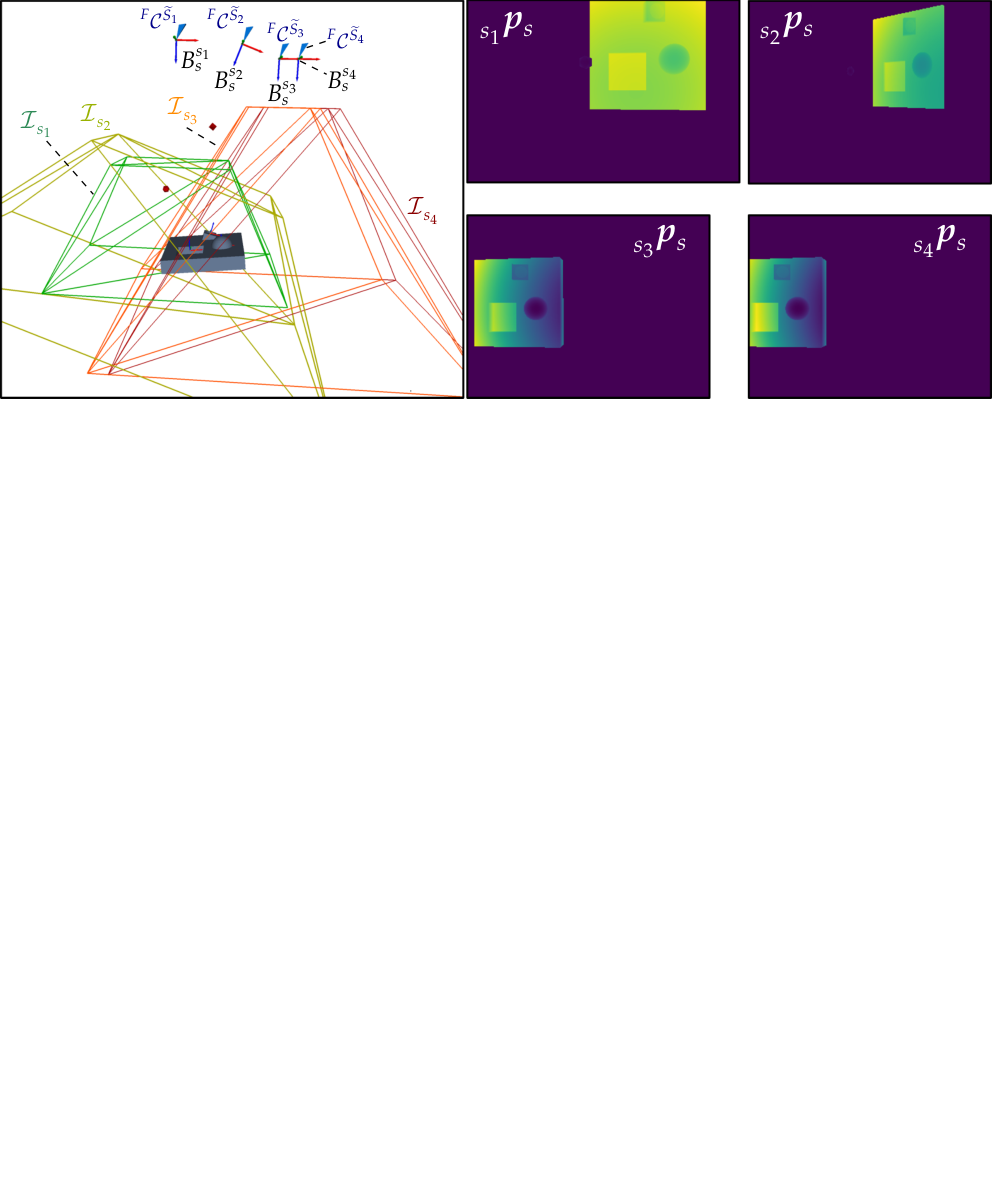
VIII-A2 Results
Following the strategy described in Algorithm 6, the joint s of the four imaging devices, i.e., , , , and were computed for acquiring all features considering all viewpoint constraints from Table III. Figure 24 shows the complexity of the described case comprising three features and some of the resulting s. The blue manifold represents the final constrained space of the first imaging device . It can be appreciated that is characterized by the intersection of all other s. Moreover, Fig. 24 shows that the manifold is mainly constrained by the corresponding to the second range sensor, i.e., .
To verify the validity of the computed s, the depth images and point clouds for all imaging devices at eight extreme viewpoints were rendered. Figure 25 shows the corresponding rendered scene and resulting depth images for each imaging device at one extreme viewpoint . The depth images demonstrate that all imaging device can successfully acquire all features without occlusion simultaneously.
The total computation time for characterizing all s corresponded to . However, this time comprises other computation steps (e.g., frames transformation and inverse kinematic operations using ROS-Services), which distort the effective computation time of the s. A proper analysis of the computational efficiency of the whole strategy remains to be further investigated.
VIII-A3 Summary
Despite the complexity of the use case, the framework (models, methods, and integration strategy) presented within this paper demonstrated its effectiveness in characterize a continuous topological space in the special Euclidean, where all defined viewpoint constraints could be fulfilled. The simulated depth-images and point clouds confirmed that all selected viewpoints within the characterized satisfied all regarded constraints. Moreover, the proposed academic example effectively outlines a simple but sufficient complex scenario to benchmark our and future viewpoint planning strategies.
VIII-B Real Experimental Analysis
To assess the usability and validity of our framework within real applications, the framework presented in this study was utilized to generate automatically valid viewpoints for capturing different features of a car door using real RVS, i.e., the AIBox from ZEISS. The AIBox is an industrial measurement cell used to automate different vision-based quality inspection tasks such as dimensional metrology and digitization, among others.
VIII-B1 System Description
The AIBox is an integrated industrial RVS, equipped with a structured light sensor (ZEISS COMET PRO AE), a six-axis industrial robot (Fanuc M-20ia), and a rotary table for mounting an inspection object. Moreover, to evaluate the use of our approach considering a multisensor system, we additionally attached a stereo sensor (rc_visard 65, Roboception) to the structured light sensor. The imaging parameters of both sensors are given in Table II. Figure 26 provides an overview of the reconfigured AIBox with the stereo sensor. We assume that the inspection object is roughly aligned, e.g., in [67] we presented a CNN fully trained on synthetic data to automate this task using the RVS sensor.
VIII-B2 Vision Task Definition
The validation of our framework was performed on the basis of two vision tasks considering diverse viewpoint constraints. For the first task, we considered just the ZEISS sensor to acquire the features , which lie on the outside of the door and can be potentially occluded by the door fixture. For the second task, we considered both sensors and the acquisition of two features on the inside of the door. The incidence angle for the first case corresponded to a sensor orientation of and for the second of . To compensate any kinematic modeling uncertainties, we consider an overall kinematic error of for and of for and .
VIII-B3 Results
For both vision tasks we computed the necessary s aligned to the strategy presented by Algorithm 6. The s of the first inspection scenario for the camera and projector of the Comet Pro AE and its corresponding occlusion spaces are displayed on the left image of Figure 27. To assess the validity of the characterized s, we chose diverse extreme viewpoints at the vertices of the manifold and performed real measurements. On the right side of Figure 27 the real monochrome images of the camera and the resulting point clouds at two validating viewpoints are displayed. The 2D images and point clouds prove that both features can be successfully acquired from these both viewpoints, which confirms the free sight for the sensor and the illumination of both features without shadows.
Moreover, on the left of Figure 28 the constrained spaces of the first imaging device of each sensor, i.e., and , are visualized for the second inspection scenario. Analogously to the first scenario, two extreme viewpoints at the vertices of the manifolds were selected to assess the validity of the computed s. As expected, the real 2D images of all imaging devices and the resulting point clouds of both sensors at two exemplary extreme viewpoints (shown on the right of Figure 27) demonstrate that all features can be successfully acquired by the four imaging devices of both sensors.
VIII-B4 Summary
Using an industrial RVS, and regarding real viewpoint constraints, we were able to validate the formulations, characterization, and application of s for inspection tasks in an industrial context. These experiments show the suitability of our framework for an industrial application on a real RVS with multiple range sensors.
Furthermore, our strategy for merging individual s to capture more than one feature proved to be effective for the regarded vision tasks. However, a more complex task such as the inspection of all door features requires a more complex strategy, which considers the search of features that can be acquired together. This question recalls the overall VPP, which falls outside the scope of this publication and we intend to address in our future work.


IX Summary and Outlook
IX-A Summary
The computation of valid viewpoints considering different system constraints, named VGP in this publication, is considered a complex and unsolved challenge that lacks a generic and holistic framework for its proper formulation and resolution. In this paper, we outline the VGP as a geometric problem that can be solved explicitly in the special Euclidean using suitable and explicit models of all related domains of an RVS and viewpoint constraints. Within this context, much of our effort was devoted to the comprehensive and systematic formulation of the VGP and the exhaustive characterization of domains and viewpoint constraints aligned to the formulation of geometric problems.
The core result of this study is the characterization of s, which can be understood as topological manifolds that span a space with infinite viewpoint solutions to acquire one feature or a group of features considering various viewpoint constraints and modeling uncertainties. Our approach focuses on providing rather infinite valid solutions instead of optimal ones. If the entire a priori knowledge of the RVS can be formalized and integrated into the , then it we can assume that any viewpoint within it is a local optimum. Our work shows that a handful of viewpoint constraints can be efficiently and simply modeled geometrically and integrated in a common framework to span such constrained spaces. Finally, based on a comprehensive academic example and a real application, we demonstrate the usability of such a framework.
IX-B Limitations and Chances
We are aware that the framework proposed in the present study may have some limitations that may prevent its straightforward application for other RVS or use-cases. First, it must be regarded that our framework can be classified under the category of model-based approaches. Therefore, in a first step a priori information to model the components of the considered RVS must be regarded. We consider that an exhaustive and explicit modeling of the necessary domains is necessary for delivering solutions that offer a higher generalization for other applications and systems. For the benefit of generalization, complexity reduction, and computational efficiency we regarded various simplifications, which could affect the accuracy of some models and might yield more conservative, however, more robust solutions.
We firmly believe that the VGP can be efficiently solved geometrically. We demonstrated that many constraints can be explicitly and efficiently characterized by combining several techniques, including linear algebra, trigonometry, and geometrical analysis. In the scope of our experiments, we confirmed that the computation of the s manifolds based on these approaches ran efficiently in linear times. However, we also noted that algorithms comprising CSG Boolean operations are more computationally expensive, especially on calculations considering multiple Boolean operations on the same manifold. Although this limitation can be minimized by filtering and smoothing algorithms for decimating manifolds, this characteristic could still be considered insufficient for some users and applications. Although the shortcomings of CSG Boolean techniques regarding their computational efficiency have been mentioned in some prior works, we also believe that the present available computational performance and paralleling capabilities of CPUs and GPUs require a new reevaluation of their overall performance. Additionally, our work also suggests that combined with efficient imaging processing libraries, approaches requiring heavy use of CSG operations can be efficiently used within many applications. Nevertheless, a comprehensive computational efficiency analysis to find a break-even point between our approach and others remains to be further investigated.
Moreover, we also see room for improvement to increase the efficiency of some of the algorithms presented. For instance, the computation of the occlusion space and integration of constraints could also be improved using an alternative strategy and more efficient algorithms implemented in low-level programming languages. Additionally, we also see potential for improving the efficiency of some algorithms. For instance, the performance of many algorithms could enormously benefit of computational optimization techniques such as parallelization and GPU computation. For replication purposes of our work, we encourage the reader to make a thorough evaluation of the performance of the state-of-the-art libraries available at the present time, according to their application needs and system requirements.
IX-C Outlook
We consider the use of s appropriate, but not limited to vision tasks that rely on features. For example, we showed how our concept could be extended to applications that generally would not consider features and demonstrate its application for an object detection problem with a certain level of spatial uncertainty. Our ongoing work concentrates on assessing further applications or systems that may benefit from our approach, e.g., feature-based robot calibration or adaption to laser sensors. Further studies should still be undertaken in this direction to verify the usability and explore the limitations of our framework within other applications and RVSs.
Recalling that we neglected any sensor parameters that may directly constrain the , e.g., exposure time, gain, and others, we consider some other lines of research that integrate such a parameter space in the . For instance, our ongoing study investigates the combination of a data-based approach to optimize the exposure times and the use of s for finding optimized sensor poses.
The most promising future research should be devoted to the overall problem of the VPP, which could be reformulated based on the present study and its findings. Further research that will exploit this and comprises a holistic strategy for its resolution is already in progress.
We believe that our work will serve as a solid base and guideline for further studies to adapt and extend our framework according to the individual requirements of their concrete applications and RVS.
Acknowledgments
The framework presented in this paper was developed and thoroughly evaluated within the scope of the “CyMePro” (Cyber-physical measurement technology for 3D digitization in the networked production) project, which was funded by the Bavarian Ministry of Economic Affairs, Regional Development and Energy (funding code ESB036 / 001).
We thank our research partners AUDI AG and Carl Zeiss Optotechnik GmbH for the fruitful discussions and their cooperation. Moreover, we are deeply grateful to our colleagues Daria Leiber for the fruitful discussions regarding the initial drafting and Benedikt Schmucker for the critical revision of the present publication.
References
- [1] Danica Kragic and Kostas Daniilidis “3-D Vision for Navigation and Grasping” In Springer Handbook of Robotics Cham: Springer International Publishing, 2016, pp. 811–824 DOI: 10.1007/978-3-319-32552-1_32
- [2] Manon Peuzin-Jubert et al. “Survey on the View Planning Problem for Reverse Engineering and Automated Control Applications” In Computer-Aided Design 141, 2021, pp. 103094 DOI: 10.1016/j.cad.2021.103094
- [3] Petra Gospodneti\’c, Dennis Mosbach, Markus Rauhut and Hans Hagen “Viewpoint placement for inspection planning” In Machine Vision and Applications 33.1, 2022 DOI: 10.1007/s00138-021-01252-z
- [4] Shengyong Chen, Youfu Li and Ngai Kwok “Active vision in robotic systems: A survey of recent developments” In The International Journal of Robotics Research 30.11, 2011, pp. 1343–1377 DOI: 10.1177/0278364911410755
- [5] Konstantinos. Tarabanis, Peter. Allen and Roger. Tsai “A survey of sensor planning in computer vision” In IEEE transactions on Robotics and Automation 11.1, 1995, pp. 86–104
- [6] Chee Tan, Rosmiwati Mohd-Mokhtar and Mohd Arshad “A Comprehensive Review of Coverage Path Planning in Robotics Using Classical and Heuristic Algorithms” In IEEE Access 9, 2021, pp. 119310–119342 DOI: 10.1109/ACCESS.2021.3108177
- [7] K.. Tarabanis, R.. Tsai and P.. Allen “The MVP sensor planning system for robotic vision tasks” In IEEE transactions on Robotics and Automation 11.1, 1995, pp. 72–85 DOI: 10.1109/70.345939
- [8] William. Scott, Gerhard Roth and Jean-Francois Rivest “View planning for automated three-dimensional object reconstruction and inspection” In ACM Computing Surveys (CSUR) 35.1, 2003, pp. 64–96 DOI: 10.1145/641865.641868
- [9] Aaron Mavrinac and Xiang Chen “Modeling Coverage in Camera Networks: A Survey” In International Journal of Computer Vision 101.1, 2013, pp. 205–226 DOI: 10.1007/s11263-012-0587-7
- [10] Julien Kritter, Mathieu Br\’evilliers, Julien Lepagnot and Lhassane Idoumghar “On the optimal placement of cameras for surveillance and the underlying set cover problem” In Applied Soft Computing 74, 2019, pp. 133–153 DOI: 10.1016/j.asoc.2018.10.025
- [11] William. Scott “Performance-oriented view planning for automated object reconstruction”, 2002
- [12] Cregg. Cowan and Peter. Kovesi “Automatic sensor placement from vision task requirements” In IEEE Transactions on Pattern Analysis and machine intelligence 10.3, 1988, pp. 407–416 DOI: 10.1109/34.3905
- [13] C.. Cowan and A. Bergman “Determining the camera and light source location for a visual task” In Proceedings, 1989 International Conference on Robotics and Automation IEEE Comput. Soc. Press, 1989, pp. 509–514 DOI: 10.1109/ROBOT.1989.100037
- [14] K. Tarabanis and R.. Tsai “Computing occlusion-free viewpoints” In Proceedings 1992 IEEE Computer Society Conference on Computer Vision and Pattern Recognition IEEE Comput. Soc. Press, 1992, pp. 802–807 DOI: 10.1109/CVPR.1992.223168
- [15] K. Tarabanis, R.. Tsai and A. Kaul “Computing occlusion-free viewpoints” In IEEE Transactions on Pattern Analysis and machine intelligence 18.3, 1996, pp. 279–292 DOI: 10.1109/34.485556
- [16] Steven Abrams, Peter. Allen and Konstantinos Tarabanis “Computing Camera Viewpoints in an Active Robot Work Cell” In The International Journal of Robotics Research 18.3, 1999, pp. 267–285 DOI: 10.1177/02783649922066204
- [17] Michael Reed “Solid model acquisition from range imagery”, 1998
- [18] M.. Reed and P.. Allen “Constraint-based sensor planning for scene modeling” In IEEE Transactions on Pattern Analysis and machine intelligence 22.12, 2000, pp. 1460–1467 DOI: 10.1109/34.895979
- [19] Glenn. Tarbox and Susan. Gottschlich “IVIS: An integrated volumetric inspection system” In Computer Vision and Image Understanding 61.3, 1994, pp. 430–444 DOI: 10.1109/CADVIS.1994.284498
- [20] Glenn. Tarbox and Susan. Gottschlich “Planning for complete sensor coverage in inspection” In Computer Vision and Image Understanding 61.1, 1995, pp. 84–111 DOI: 10.1006/cviu.1995.1007
- [21] William. Scott “Model-based view planning” In Machine Vision and Applications 20.1, 2009, pp. 47–69 DOI: 10.1007/s00138-007-0110-2
- [22] Marc Gronle and Wolfgang Osten “View and sensor planning for multi-sensor surface inspection” In Surface Topography: Metrology and Properties 4.2, 2016, pp. 024009 DOI: 10.1088/2051-672X/4/2/024009
- [23] Wei Jing et al. “Sampling-based coverage motion planning for industrial inspection application with redundant robotic system” In 2017 IEEE/RSJ International Conference on Intelligent Robots and Systems (IROS) IEEE, 2017, pp. 5211–5218 DOI: 10.1109/IROS.2017.8206411
- [24] Dennis Mosbach et al. “Feature-Driven Viewpoint Placement for Model-Based Surface Inspection” In Machine Vision and Applications 32.1, 2021 DOI: 10.1007/s00138-020-01116-y
- [25] Emanuele Trucco, M. Umasuthan, A.. Wallace and V. Roberto “Model-based planning of optimal sensor placements for inspection” In IEEE transactions on Robotics and Automation 13.2, 1997, pp. 182–194 DOI: 10.1109/70.563641
- [26] R. Pito “A solution to the next best view problem for automated surface acquisition” In IEEE Transactions on Pattern Analysis and machine intelligence 21.10, 1999, pp. 1016–1030 DOI: 10.1109/34.799908
- [27] Dirk St\"oel et al. “Feature and viewpoint selection for industrial car assembly” In Joint Pattern Recognition Symposium, 2004, pp. 528–535
- [28] Marc. Ellenrieder, Lars Kr\"uger, Dirk St\"oel and Marc Hanheide “A versatile model-based visibility measure for geometric primitives” In Scandinavian Conference on Image Analysis, 2005, pp. 669–678
- [29] Roberto Raffaeli, Maura Mengoni, Michele Germani and Ferruccio Mandorli “Off-line view planning for the inspection of mechanical parts” In International Journal on Interactive Design and Manufacturing (IJIDeM) 7.1, 2013, pp. 1–12 DOI: 10.1007/s12008-012-0160-1
- [30] T. Kouteck\’y, D. Palousek and J. Brandejs “Sensor planning system for fringe projection scanning of sheet metal parts” In Measurement 94, 2016, pp. 60–70
- [31] Kwan. Lee and Hyun-pung Park “Automated inspection planning of free-form shape parts by laser scanning” In Robotics and Computer-Integrated Manufacturing 16.4, 2000, pp. 201–210
- [32] William Derigent et al. “3D Digitizing Strategy Planning Approach Based on a CAD Model” In Journal of Computing and Information Science in Engineering 7.1, 2006, pp. 10–19 DOI: 10.1115/1.2410023
- [33] William Tekouo Moutchiho “A New Programming Approach for Robot-based Flexible Inspection Systems”, 2012
- [34] Johnny Park, Priya. Bhat and Avinash. Kak “A Look-up Table Based Approach for Solving the Camera Selection Problem in Large Camera Networks” In Proceedings of the International Workshop on Distributed Smart Cameras ., 2006, pp. 72–76
- [35] H. Gonz\’alez-Banos “A randomized art-gallery algorithm for sensor placement” In Proceedings of the seventeenth annual symposium on Computational geometry - SCG ’01 New York, New York, USA: ACM Press, 2001, pp. 232–240 DOI: 10.1145/378583.378674
- [36] S.. Chen and Y.. Li “Automatic sensor placement for model-based robot vision” In IEEE transactions on systems, man, and cybernetics. Part B, Cybernetics : a publication of the IEEE Systems, Man, and Cybernetics Society 34.1, 2004, pp. 393–408 DOI: 10.1109/TSMCB.2003.817031
- [37] Ugur Erdem and Stan Sclaroff “Automated camera layout to satisfy task-specific and floor plan-specific coverage requirements” In Computer Vision and Image Understanding 103.3, 2006, pp. 156–169 DOI: 10.1016/j.cviu.2006.06.005
- [38] Aaron Mavrinac, Xiang Chen and Jose Alarcon-Herrera “Semiautomatic Model-Based View Planning for Active Triangulation 3-D Inspection Systems” In IEEE/ASME Transactions on Mechatronics 20.2, 2015, pp. 799–811 DOI: 10.1109/TMECH.2014.2318729
- [39] Emile Glorieux, Pasquale Franciosa and Dariusz Ceglarek “Coverage path planning with targetted viewpoint sampling for robotic free-form surface inspection” In Robotics and Computer-Integrated Manufacturing 61, 2020, pp. 101843 DOI: 10.1016/j.rcim.2019.101843
- [40] S.. Chen and Y.. Li “Vision sensor planning for 3-D model acquisition” In IEEE transactions on systems, man, and cybernetics. Part B, Cybernetics : a publication of the IEEE Systems, Man, and Cybernetics Society 35.5, 2005, pp. 894–904 DOI: 10.1109/TSMCB.2005.846907
- [41] J. Vasquez-Gomez, L. Sucar, Rafael Murrieta-Cid and Efrain Lopez-Damian “Volumetric Next-best-view Planning for 3D Object Reconstruction with Positioning Error” In International Journal of Advanced Robotic Systems 11.10, 2014, pp. 159 DOI: 10.5772/58759
- [42] Simon Kriegel, Christian Rink, Tim Bodenm\"uller and Michael Suppa “Efficient next-best-scan planning for autonomous 3D surface reconstruction of unknown objects” In Journal of Real-Time Image Processing 10.4, 2015, pp. 611–631 DOI: 10.1007/s11554-013-0386-6
- [43] Mikko Lauri, Joni Pajarinen, Jan Peters and Simone Frintrop “Multi-Sensor Next-Best-View Planning as Matroid-Constrained Submodular Maximization” In IEEE Robotics and Automation Letters 5.4, 2020, pp. 5323–5330 DOI: 10.1109/LRA.2020.3007445
- [44] Kenneth. Waldron and James Schmiedeler “Kinematics” In Springer Handbook of Robotics Cham: Springer International Publishing, 2016, pp. 11–36 DOI: 10.1007/978-3-319-32552-1_2
- [45] J\"urgen Beyerer, Fernando Puente Le\’on and Christian Frese “Machine Vision” Berlin, Heidelberg: Springer Berlin Heidelberg, 2016 DOI: 10.1007/978-3-662-47794-6
- [46] J.E Beasley and P.C Chu “A genetic algorithm for the set covering problem” In European Journal of Operational Research 94.2, 1996, pp. 392–404 DOI: 10.1016/0377-2217(95)00159-X
- [47] Anurag Mittal and Larry. Davis “A General Method for Sensor Planning in Multi-Sensor Systems: Extension to Random Occlusion” In International Journal of Computer Vision 76.1, 2007, pp. 31–52 DOI: 10.1007/s11263-007-0057-9
- [48] Mustafa Kaba, Mustafa Uzunbas and Ser Lim “A Reinforcement Learning Approach to the View Planning Problem” In 2017 IEEE Conference on Computer Vision and Pattern Recognition (CVPR), 2017, pp. 5094–5102 DOI: 10.1109/CVPR.2017.541
- [49] Tom\’as Lozano-P\’erez “Spatial Planning: A Configuration Space Approach” In Autonomous Robot Vehicles New York, NY: Springer New York, 1990, pp. 259–271 DOI: 10.1007/978-1-4613-8997-2_20
- [50] Jean-Claude Latombe “Robot Motion Planning” 124, The Springer International Series in Engineering and Computer Science, Robotics Boston, MA: Springer, 1991 DOI: 10.1007/978-1-4615-4022-9
- [51] Steven LaValle “Planning algorithms” Cambridge: Cambridge University Press, 2006
- [52] Malik Ghallab, Dana. Nau and Paolo Traverso “Automated planning” San Francisco, Calif.: Morgan KaufmannOxford : Elsevier Science, 2004
- [53] Thom Fr\"uhwirth and Slim Abdennadher “Essentials of constraint programming”, Cognitive technologies BerlinLondon: Springer, 2011
- [54] Morgan Quigley et al. “ROS: an open-source Robot Operating System” In ICRA workshop on open source software 3, 2009, pp. 5
- [55] Alejandro Maga\˜na, Philipp Bauer and Gunther Reinhart “Concept of a learning knowledge-based system for programming industrial robots” In Procedia CIRP 79, 2019, pp. 626–631 DOI: 10.1016/j.procir.2019.02.076
- [56] Alejandro Maga\˜na, Silvia Gebel, Philipp Bauer and Gunther Reinhart “Knowledge-Based Service-Oriented System for the Automated Programming of Robot-Based Inspection Systems” In 2020 25th IEEE International Conference on Emerging Technologies and Factory Automation (ETFA) IEEE, 2020, pp. 1511–1518 DOI: 10.1109/ETFA46521.2020.9212033
- [57] Qingnan Zhou, Eitan Grinspun, Denis Zorin and Alec Jacobson “Mesh arrangements for solid geometry” In ACM Transactions on Graphics 35.4, 2016, pp. 1–15 DOI: 10.1145/2897824.2925901
- [58] Trimesh “trimesh” trimesh, 2022 URL: https://trimsh.org/
- [59] Ingo Wald et al. “Embree” In ACM Transactions on Graphics 33.4, 2014, pp. 1–8 DOI: 10.1145/2601097.2601199
- [60] Unity Technologies “Unity” Unity Technologies, 2022 URL: https://unity.com/
- [61] Martin Bischoff “ROS#” https://github.com/siemens/ros-sharp: Siemens AG, 2022 URL: https://github.com/siemens/ros-sharp
- [62] Scott. Roth “Ray casting for modeling solids” In Computer Graphics and Image Processing 18.2, 1982, pp. 109–144 DOI: 10.1016/0146-664X(82)90169-1
- [63] Andrew. Glassner “An Introduction to ray tracing” London: Academic, 1989
- [64] H. Edelsbrunner, D. Kirkpatrick and R. Seidel “On the shape of a set of points in the plane” In IEEE Transactions on Information Theory 29.4, 1983, pp. 551–559 DOI: 10.1109/TIT.1983.1056714
- [65] Michael Kazhdan, Matthew Bolitho and Hugues Hoppe “Poisson Surface Reconstruction” In Proceedings of the Fourth Eurographics Symposium on Geometry Processing, SGP ’06 Goslar, DEU: Eurographics Association, 2006, pp. 61–70
- [66] Philipp Bauer et al. “Registration strategy of point clouds based on region-specific projections and virtual structures for robot-based inspection systems” In Measurement 185, 2021, pp. 109963 DOI: 10.1016/j.measurement.2021.109963
- [67] Alejandro Maga\˜na, Hang Wu, Philipp Bauer and Gunther Reinhart “PoseNetwork: Pipeline for the Automated Generation of Synthetic Training Data and CNN for Object Detection, Segmentation, and Orientation Estimation” In 2020 25th IEEE International Conference on Emerging Technologies and Factory Automation (ETFA) IEEE, 2020, pp. 587–594 DOI: 10.1109/ETFA46521.2020.9212064
| General Requirement | Description |
| 1. Generalization | The models and approaches used should be abstracted and generalized in the best possible level so that they can be used for different components of an RVS and can be applied to solve a broad range of vision tasks. |
| 2. Computational Efficiency | The methods and techniques used should strive a low level of computational complexity. Whenever possible, analytical and linear models should be preferred over complex techniques, such as stochastic and heuristic algorithms. Nevertheless, considering offline scenarios the trade-off between computing a good enough solution within an acceptable amount of time should be individually assessed. |
| 3. Determinism | Due to traceability and safety issues within industrial applications deterministic approaches should be prioritized. |
| 4. Modularity and Scalability | The approaches and models should consider in general a modular structure and promote their scalability. |
| 5. Limited A-priori Knowledge | The parameters required to implement the models and approaches should be easily accessible for the end-users. Neither in-depth optics nor robotic knowledge should be required. |
| Notation | Index Description |
| variable, parameter, vector, frame or transformation | |
| RVS domain, i.e., sensor, robot, feature, object, environment or d element of a list or set | |
| related domain, additional notation or depending variable | |
| base frame of the coordinate system or space of feature | |
| origin frame of the coordinate system | |
| Notes | The indexes and just apply for pose vectors, frames and transformations. |
| Example | The index notation can be better understood consider following examples: • : Let the geometry of a feature be described by a surface point • : If the feature comprises more surface points, then let the point with the index be denoted by . • : Assuming that the position of a surface point is described in the coordinate system of the feature, , then it follows: . In case that the base coordinate frame has the same notation as the domain itself, i.e. , then just the index for the domain is given: . • : In case that the frame of the surface point is given in the coordinate reference system of the object , then following notation applies: . |
| Symbol | Description |
| General | |
| Viewpoint constraint | |
| Set of viewpoint constraints | |
| Feature | |
| Set of features | |
| imaging device of sensor | |
| Viewpoint | |
| Sensor pose in | |
| Spatial Dimensions | |
| Frame | |
| Translation vector in | |
| Orientation matrix in | |
| Manifold vertex in | |
| Topological Spaces | |
| for a set of viewpoint constraints | |
| i of the viewpoint constraint | |
| Frustum space |
| Feature | , | |||||
| Topology | Point | Slot | Circle | Half-Sphere | Icosahedron | Octaeder |
| Generalized Topology | - | Square | Square | Cube | - | - |
| Dimensions in mm | , | , | edge length: | edge length: | ||
| Translation vector in object’s frame in mm | ||||||
| Rotation in Euler Angles in object’s frame in ∘ |
| Rotation around y-Axis | Rotation around x-Axis | |||||||
| Vertex of | ||||||||
| 1 | ||||||||
| 2 | ||||||||
| 3 | ||||||||
| 4 | ||||||||
| 5 | ||||||||
| 6 | ||||||||
| 7 | ||||||||
| 8 | ||||||||
- 1.
Considering the simplification of the feature topology (cf. III-D3) let a set of view rays denoted by be shot at each feature corner point with following direction vectors :
- 2.
The direction vectors are characterized by a grid of equidistant rays, which can be expressed by means of the aperture angles and :
The maximal aperture angles and can simply correspond to the FOV angles of the sensor. An efficient alternative is to consider the aperture angles , which already comprises the FOV angles and other constraints. The total number of rays depends on the chosen step size for computing the equidistant view rays:

